How to Train Unstable Looped Tensor Network

Abstract

A rising problem in the compression of Deep Neural Networks is how to reduce the number of parameters in convolutional kernels and the complexity of these layers by low-rank tensor approximation. Canonical polyadic tensor decomposition (CPD) and Tucker tensor decomposition (TKD) are two solutions to this problem and provide promising results. However, CPD often fails due to degeneracy, making the networks unstable and hard to fine-tune. TKD does not provide much compression if the core tensor is big. This motivates using a hybrid model of CPD and TKD, a decomposition with multiple Tucker models with small core tensor, known as block term decomposition (BTD). This paper proposes a more compact model that further compresses the BTD by enforcing core tensors in BTD identical. We establish a link between the BTD with shared parameters and a looped chain tensor network (TC). Unfortunately, such strongly constrained tensor networks (with loop) encounter severe numerical instability, as proved by [1] and [2]. We study perturbation of chain tensor networks, provide interpretation of instability in TC, demonstrate the problem. We propose novel methods to gain the stability of the decomposition results, keep the network robust and attain better approximation. Experimental results will confirm the superiority of the proposed methods in compression of well-known CNNs, and TC decomposition under challenging scenarios.

1 Introduction

Despite the outstanding efficiency of convolutional neural networks (CNNs), their practical application is hampered by computational complexity and high resources consumption. Based on the observation that the weights of convolutional networks contain redundant information, they can be compressed without large losses in network performance by structural pruning [3], sparsification [4], quantization [5] and low-rank approximation [6, 7, 8]. Prior works have explored a wide variety of methods to weight factorization [9]: singular value decomposition [7], Canonical Polyadic decomposition [8], Tucker decomposition [6] and Tensor Train decomposition [10, 11].

Canonical polyadic tensor decomposition (CPD) was the first low-rank model applied to compress CNN [12]. The CP-convolutional layer composes separable convolution kernel matrices. CPD often encounters degeneracy, the estimated model is sensitive to a slight change of the parameters; this makes the entire CNN unstable.

Tucker-2 decomposition (TKD2) [13]. An alternative method [14] is to compress the input and output dimensions of the convolutional kernel, $\boldsymbol{\mathscr{{Y}}}=\boldsymbol{\mathscr{{B}}}\times_{1}{\bf A}\times_{3}{\bf C}$ (see Figure 1(a)). Compared to CPD, TKD is more stable, and the ranks of the decomposition can be determined using SVD or VBMF. However, in practice, the dimensions of input and output modes in TKD can be large and make the compression less efficient than CPD.

Block-term decomposition (BTD) [15] is a hybrid of CPD and TKD, constrains the core tensor $\boldsymbol{\mathscr{{G}}}$ to be sparse, block diagonal, and thereby BTD comprises a smaller number of parameters than TKD. More precisely, BTD models the data as sum of multiple Tucker terms,

$$\boldsymbol{\mathscr{{Y}}}=\sum_{t=1}^{T}\boldsymbol{\mathscr{{B}}}_{t}\times_{1}{\bf A}_{t}\times_{3}{\bf C}_{t}$$ (1)

where $\boldsymbol{\mathscr{{B}}}_{t}$ are order-3 core tensors of size $R_{t}\times I_{2}\times S_{t}$, ${\bf A}_{t}$ and ${\bf C}_{t}$ are factor matrices of size $I_{1}\times R_{t}$ and $I_{3}\times S_{t}$, respectively, $t=1,\ldots,T$. So far, there are no available proper selection criteria of the block size (rank of BTD) and the number of terms.

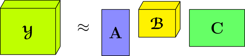
(a) TKD

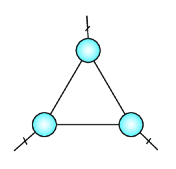
(b) TC

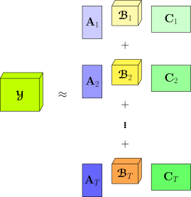
(c) BTD

Figure 1: Approximation of an order-3 tensor using (a) TKD-2, or (c) BTD, comprising multiple TKDs (c). BTD with shared core tensors, $\boldsymbol{\mathscr{{B}}}_{1}=\ldots=\boldsymbol{\mathscr{{B}}}_{T}$, forms the Tensor Chain(b).

BTD with shared core tensors. In this paper, we propose a BTD with shared core tensors to reduce parameters in BTD, see illustration in Figure 1(c). In particular case, all core tensors are identical, i.e., $\boldsymbol{\mathscr{{B}}}_{1}=\ldots=\boldsymbol{\mathscr{{B}}}_{T}$. We will show that this parameter-shared BTD is equivalent to a looped tensor network (Tensor chain - TC)[16, 17]. Using this connection, we propose a sensitivity correction procedure to overcome the problem with instability in this class of tensor models.

Such strongly constrained BTD or TC is not closed, i.e., the set of TC tensors of a fixed rank (bond dimension) is not Zariski closed. The openness of the set of fixed rank-r tensors implies that for some rank-$r$ tensors, one can approximate it with arbitrary precision by a tensor of a smaller rank $r_{b}$. For the canonical rank, the smallest rank $r_{b}$ is called the border rank of the tensor. For TC, we refer to Section 3, “Closedness of tensor network formats” in [17], and the work of [18], which addresses the question of L. Grasedyck arising in quantum information theory, whether a tensor network containing a cycle (loop) is Zariski closed. One of the important conclusions is that “if the tensor network graph $G$ is not a tree (it contains cycles), then the induced tensor network $U_{G}$ is in general not closed”, see [18], also Remark 2.1.12. Ph.D. thesis, [2]. The looped TN leads to severe numerical instability problem in finding the best approximation, see Theorem 14.1.2.2[1] and [2].

Contributions. The problem of instability in the TC model was identified early in [17, 2]. However, the problem is not well understood, and there is no method to deal with it. In this paper, we will study the sensitivity in TC and illustrate this type of degeneracy. We propose novel methods to stabilize the estimated TC results and introduce a new TC layer or shared-parameters BTD convolutional layer. Finally, our primary aim is to propose a new convolutional layer with kernel in the form of TC or BTD with shared core tensors. The proposed algorithms in this paper can be applied to tensor decomposition in other applications.

We provide results of extensive experiments to confirm the efficiency of the proposed algorithms. Particularly, we empirically show that the neural network with weights in TC format obtained using our algorithms is more stable during fine-tuning and recovers faster (close) to initial accuracy.

2 Looped Tensor Network - Tensor Chain

For simplicity, we first present TC for order-3 data. Extension of TC to higher-order tensor can be made straightforwardly. [16, 17] introduced the looped Tensor Chain as an extension of the Tensor Train (TT)[19]. Since there are no first and last core tensors, TC is expected to overcome the imbalance rank issue in TT decomposition. Tensor Ring is the same tensor network model inspired by Tensor Chain. See illustration in Figure 1(b). We use the name Tensor Chain to honor the original authors who have invented it. The TC for an order-3 tensor $\boldsymbol{\mathscr{{Y}}}$ of size $I_{1}\times I_{2}\times I_{3}$ reads

$$\boldsymbol{\mathscr{{Y}}}=\sum_{r_{1}=1}^{R_{1}}\,\sum_{r_{2}=1}^{R_{2}}\sum_{r_{3}=1}^{R_{3}}\boldsymbol{\mathscr{{A}}}(r_{1},:,r_{2})\circ\boldsymbol{\mathscr{{B}}}(r_{2},:,r_{3})\circ\boldsymbol{\mathscr{{C}}}(r_{3},:,r_{1}),$$ (2)

where ‘$\circ$’ represents the outer product, $\boldsymbol{\mathscr{{A}}}$, $\boldsymbol{\mathscr{{B}}}$ and $\boldsymbol{\mathscr{{C}}}$ are core tensors of size $R_{1}\times I_{1}\times R_{2}$, $R_{2}\times I_{2}\times R_{3}$, $R_{3}\times I_{3}\times R_{1}$, respectively, and its element can write as $y_{ijk}=\mathop{\rm tr}\nolimits({\boldsymbol{\mathscr{{A}}}(:,i,:)\boldsymbol{\mathscr{{B}}}(:,j,:)\boldsymbol{\mathscr{{C}}}(:,k,:)})$. We use shorthand notation for TC as $\boldsymbol{\mathscr{{Y}}}=\mathopen{{\stackengine{.25ex}{[}{{\scaleto{\circlearrowright}{1.1ex}}}{O}{c}{F}{F}{L}}}\boldsymbol{\mathscr{{A}}},\boldsymbol{\mathscr{{B}}},\boldsymbol{\mathscr{{C}}}\mathclose{{\stackengine{.25ex}{]}{\hskip 0.86108pt{\scaleto{\circlearrowleft}{1.1ex}}}{O}{c}{F}{F}{L}}}$. The links between TC and BTD are revealed in the following Lemma.

Lemma 2.1 (Equivalence of BTD with shared core tensors and TC).

The constrained BTD with shared core tensors in (1) is a TC model $\boldsymbol{\mathscr{{Y}}}=\mathopen{{\stackengine{.25ex}{[}{{\scaleto{\circlearrowright}{1.1ex}}}{O}{c}{F}{F}{L}}}\boldsymbol{\mathscr{{A}}},\boldsymbol{\mathscr{{B}}},\boldsymbol{\mathscr{{C}}}\mathclose{{\stackengine{.25ex}{]}{\hskip 0.86108pt{\scaleto{\circlearrowleft}{1.1ex}}}{O}{c}{F}{F}{L}}}$ where $\boldsymbol{\mathscr{{A}}}$ is of size $R_{1}\times I_{1}\times R_{2}$ with slices $\boldsymbol{\mathscr{{A}}}(t,:,:)={\bf A}_{t}$, $\boldsymbol{\mathscr{{C}}}$ of size $R_{3}\times I_{3}\times R_{1}$ and $\boldsymbol{\mathscr{{C}}}(:,:,t)={\bf C}_{t}$, $t=1,\ldots,R_{1}$. (Proof is provided in Appendix B.)

The TC for a higher order tensor, $\boldsymbol{\mathscr{{Y}}}$, of size $I_{1}\times I_{2}\times\cdots\times I_{N}$ can be generalized as

$$\boldsymbol{\mathscr{{Y}}}=\sum_{r_{1}=1}^{R_{1}}\cdots\sum_{r_{N}=1}^{R_{N}}\boldsymbol{\mathscr{{A}}}_{1}(r_{1},:,r_{2})\circ\boldsymbol{\mathscr{{A}}}_{2}(r_{2},:,r_{3})\circ\cdots\circ\boldsymbol{\mathscr{{A}}}_{N}(r_{N},:,r_{1}),$$

where $\boldsymbol{\mathscr{{A}}}_{1}$, …, $\boldsymbol{\mathscr{{A}}}_{N}$ are core tensors of size $R_{n}\times I_{n}\times R_{n+1}$, $R_{N+1}=R_{1}$. We can regard TC of order-$N$ as a nested TC of order-3 whose the core tensor $\boldsymbol{\mathscr{{B}}}$ in (2) is a Tensor-Train of ($N-2$) core tensors $\boldsymbol{\mathscr{{A}}}_{2}$, …, $\boldsymbol{\mathscr{{A}}}_{N-1}$, i.e., $\boldsymbol{\mathscr{{B}}}=\boldsymbol{\mathscr{{A}}}_{2}\bullet\boldsymbol{\mathscr{{A}}}_{3}\bullet\cdots\bullet\boldsymbol{\mathscr{{A}}}_{N-1}$, where the train-contraction “$\bullet$” is defined in Appendix A.1.

2.1 Algorithms for TC decomposition

[17] proposed nonlinear block Gauss-Seidel algorithms including alternating least squares (ALS), density-matrix renormalization group (DMRG), and adaptive cross approximation for contracted tensor networks, in which TC is a special case. Thanks to links between TC and BTD, TC and structured TKD, we can also use algorithms for BTD, e.g., the nonlinear least squares (NLS) [20], Krylov-Levenberg-Marquardt (KLM) [21] algorithms or the OPT algorithm based on Limited-memory BFGS method[22].

Like other tensor decompositions, the ALS[17, 23, 2] is still considered the best algorithm for TC, especially when DMRG cannot be applied. Various variants of these two update schemes were proposed e.g., for the tensor completion problem [24, 25, 26, 27, 28, 29, 30, 31, 32], hyperspectral super-resolution [33]. For determination of bond dimensions,we refer to [34, 35]. Nevertheless, all existing TC algorithms are not robust to perturbation of parameters. For the first time, we propose the algorithm that provides optimal TC decomposition with low(est) sensitivity and considerably alleviates the problem of stacking in local minima of algorithms for TC.

2.2 Major problem: Instability

The TC was inspired by two successful models, TT and BTD, to overcome the high intermediate ranks in TT and enforce a more compact model for BTD. As mentioned earlier, [1] and [17] pointed out the problem with TC. We show that any TC model can be unstable with very high intensity and sensitivity. First, we define TC intensity.

Remark 2.2.

The TC model, $\boldsymbol{\mathscr{{Y}}}=\mathopen{{\stackengine{.25ex}{[}{{\scaleto{\circlearrowright}{1.1ex}}}{O}{c}{F}{F}{L}}}\boldsymbol{\mathscr{{A}}},\boldsymbol{\mathscr{{B}}},\boldsymbol{\mathscr{{C}}}\mathclose{{\stackengine{.25ex}{]}{\hskip 0.86108pt{\scaleto{\circlearrowleft}{1.1ex}}}{O}{c}{F}{F}{L}}}$, is not unique up to scaling

$$\boldsymbol{\mathscr{{Y}}}=\,\mathopen{{\stackengine{.25ex}{[}{{\scaleto{\circlearrowright}{1.1ex}}}{O}{c}{F}{F}{L}}}\alpha_{1}\boldsymbol{\mathscr{{A}}},\alpha_{2}\boldsymbol{\mathscr{{B}}},\alpha_{3}\boldsymbol{\mathscr{{C}}}\mathclose{{\stackengine{.25ex}{]}{\hskip 0.86108pt{\scaleto{\circlearrowleft}{1.1ex}}}{O}{c}{F}{F}{L}}}$$ (3)

with arbitrary factors $\alpha_{1}$, $\alpha_{2}$, and $\alpha_{3}$ such that $\alpha_{1}\alpha_{2}\alpha_{3}=1$.

Remark 2.3.

The TC model, $\boldsymbol{\mathscr{{Y}}}=\mathopen{{\stackengine{.25ex}{[}{{\scaleto{\circlearrowright}{1.1ex}}}{O}{c}{F}{F}{L}}}\boldsymbol{\mathscr{{A}}},\boldsymbol{\mathscr{{B}}},\boldsymbol{\mathscr{{C}}}\mathclose{{\stackengine{.25ex}{]}{\hskip 0.86108pt{\scaleto{\circlearrowleft}{1.1ex}}}{O}{c}{F}{F}{L}}}$, is also non-unique up to rotation

$$\boldsymbol{\mathscr{{Y}}}=\,\mathopen{{\stackengine{.25ex}{[}{{\scaleto{\circlearrowright}{1.1ex}}}{O}{c}{F}{F}{L}}}\boldsymbol{\mathscr{{A}}}\bullet{\bf Q},{\bf Q}^{-1}\bullet\boldsymbol{\mathscr{{B}}},\boldsymbol{\mathscr{{C}}}\mathclose{{\stackengine{.25ex}{]}{\hskip 0.86108pt{\scaleto{\circlearrowleft}{1.1ex}}}{O}{c}{F}{F}{L}}}$$ (4)

where ${\bf Q}$ is an arbitrary invertible matrix of size $R_{2}\times R_{2}$.

Definition 2.4 (TC intensity).

For a given TC model, $\boldsymbol{\mathscr{{Y}}}=\mathopen{{\stackengine{.25ex}{[}{{\scaleto{\circlearrowright}{1.1ex}}}{O}{c}{F}{F}{L}}}\boldsymbol{\mathscr{{A}}},\boldsymbol{\mathscr{{B}}},\boldsymbol{\mathscr{{C}}}\mathclose{{\stackengine{.25ex}{]}{\hskip 0.86108pt{\scaleto{\circlearrowleft}{1.1ex}}}{O}{c}{F}{F}{L}}}$, we can always normalize core tensors to unit norm, $\tilde{\boldsymbol{\mathscr{{A}}}}={\boldsymbol{\mathscr{{A}}}}/\|\boldsymbol{\mathscr{{A}}}\|_{F}$, $\tilde{\boldsymbol{\mathscr{{B}}}}={\boldsymbol{\mathscr{{B}}}}/\|\boldsymbol{\mathscr{{B}}}\|_{F}$,$\tilde{\boldsymbol{\mathscr{{C}}}}={\boldsymbol{\mathscr{{C}}}}/\|\boldsymbol{\mathscr{{C}}}\|_{F}$ then $\boldsymbol{\mathscr{{Y}}}=\alpha\,\mathopen{{\stackengine{.25ex}{[}{{\scaleto{\circlearrowright}{1.1ex}}}{O}{c}{F}{F}{L}}}\tilde{\boldsymbol{\mathscr{{A}}}},\tilde{\boldsymbol{\mathscr{{B}}}},\tilde{\boldsymbol{\mathscr{{C}}}}\mathclose{{\stackengine{.25ex}{]}{\hskip 0.86108pt{\scaleto{\circlearrowleft}{1.1ex}}}{O}{c}{F}{F}{L}}}$ where $\alpha=\|\boldsymbol{\mathscr{{A}}}\|_{F}\|\boldsymbol{\mathscr{{B}}}\|_{F}\|\boldsymbol{\mathscr{{C}}}\|_{F}$ is called the TC intensity.

Lemma 2.5 (TC Degeneracy).

For a given TC model, $\boldsymbol{\mathscr{{Y}}}=\mathopen{{\stackengine{.25ex}{[}{{\scaleto{\circlearrowright}{1.1ex}}}{O}{c}{F}{F}{L}}}\boldsymbol{\mathscr{{A}}},\boldsymbol{\mathscr{{B}}},\boldsymbol{\mathscr{{C}}}\mathclose{{\stackengine{.25ex}{]}{\hskip 0.86108pt{\scaleto{\circlearrowleft}{1.1ex}}}{O}{c}{F}{F}{L}}}$, there is always a sequence of equivalent TC models with diverging TC intensities. (Proof is provided in Appendix C.)

Remark 2.6 (TC instability).

The first observation is that TC models estimated by any iterative algorithms can encounter large TC-intensity. In many cases, the TC-intensity increases quickly with the iterations. Without proper processing, the algorithm gets stuck in a false local minimum. The decomposition is more challenging, especially when the dimension of a core tensor is smaller than its ranks, e.g., $R_{1}R_{2}>I_{1}$, or when components of the core tensors are highly collinear, or decomposition with missing entries. Such a type of degeneracy in TC happens quite often and is similar to that in CPD.

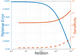
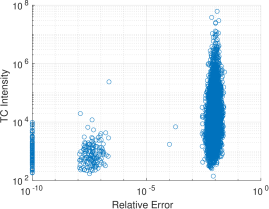
Figure 2: TC decomposition of tensors of size $7\times 7\times 7$ in Example 2. (a) Relative error of the ALS in one TC decomposition. The red solid and dashed curves show the TC sensitivity and intensity, increasing drastically during the estimation. (b) The Scatter plot shows coherence between high intensity and high approximation error (bad decomposition).

Example 1  [TC with bond dimensions exceeding tensor dimensions] We provide an illustrative example for TC degeneracy in the decomposition of noise-free synthetic tensors of size $7\times 7\times 7$ with bond dimension $(3-3-3)$, composed from 3 core tensors randomly generated. The decomposition using the ALS algorithm in 5000 iterations succeeds in less than 3% in 10000 independent TC decompositions, see Figure 2.

Why ALS and many other algorithms for TC fail? The TC intensity of the estimated tensor quickly increases after several thousand iterations, as seen in Figure 2 for illustration of relative errors in one run. The TC intensity exceeds $10^{7}$ after 10000 iterations, making the algorithm converge to local minima with a relative approximation error of 0.036. Scatter plot of intensity and relative approximation errors over 10000 TC decompositions in Figure 2 indicates coherence between bad decomposition results with high intensity. The above example shows a difficult case when core tensors, $\boldsymbol{\mathscr{{U}}}_{n}$, have fat factor matrices, ${\bf U}_{n}$, $R_{n-1}R_{n}=9>7$.

Example 2  [TC with highly collinear loading components] We decompose order-3 tensors of size $27\times 27\times 27$ which admit the TC model, $\boldsymbol{\mathscr{{Y}}}=\,\mathopen{{\stackengine{.25ex}{[}{{\scaleto{\circlearrowright}{1.1ex}}}{O}{c}{F}{F}{L}}}\boldsymbol{\mathscr{{U}}}_{1},\boldsymbol{\mathscr{{U}}}_{2},\boldsymbol{\mathscr{{U}}}_{3}\mathclose{{\stackengine{.25ex}{]}{\hskip 0.86108pt{\scaleto{\circlearrowleft}{1.1ex}}}{O}{c}{F}{F}{L}}}$, with bond dimensions $(5-5-5)$. The factor matrices ${{\bf U}}_{n}$ of size $27\times 25$ have highly collinear loading components, $0.97\leq{{\bf U}}^{T}_{n}(:,r){{\bf U}}_{n}(:,s)\leq 0.99$, $n=1,2,3$. The relative approximation errors of the ALS shown in Figure 3(a) indicate that ALS failed in this example. The intensity (dashed red curve) of the estimated TC tensors increased quickly and exceeded $2.7\times 10^{6}$, whereas its sensitivity (dotted blue curve) passed the level of $10^{6}$ after 6000 iterations as shown in Figure 3(b). The OPT(WOPT) [22] and NLS algorithms [36] also failed.

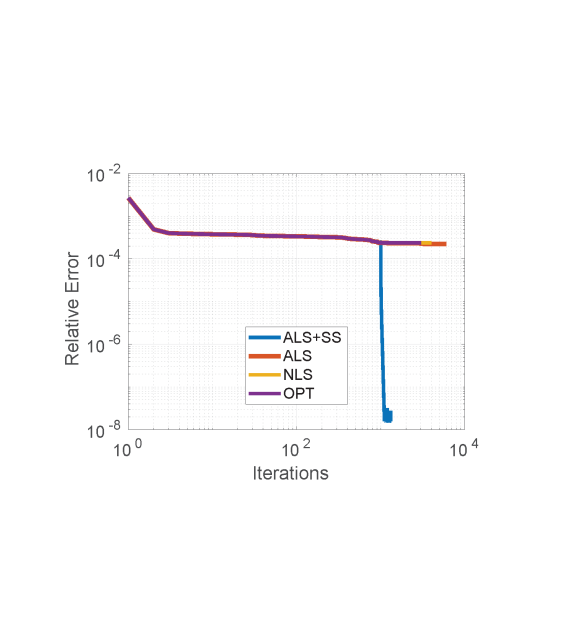
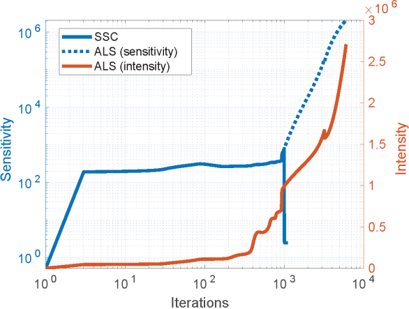
Figure 3: Illustration for performances obtained by algorithms used in Example 2. ALS+SS is the ALS with sensitivity correction. Without the SS correction, the estimated tensors have very high sensitivity and TC intensity.

Example 3  [TC for incomplete data] We demonstrate a simple TC decomposition for tensors of size $9\times 9\times 9$ with bond dimensions $(3-3-3)$. The considered tensors can be factorized quickly. However, when 50% of the tensor elements are randomly removed, the tensors are challenging to any TC algorithms. The success rate for OPT[22] and ALS is less than 11%. Figure 4 illustrates the convergence of OPT in one TC decomposition and scatter plot of the sensitivity and relative approximation errors. The algorithms get stuck in local minimal and cannot attain exact decomposition.

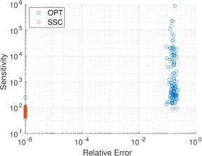
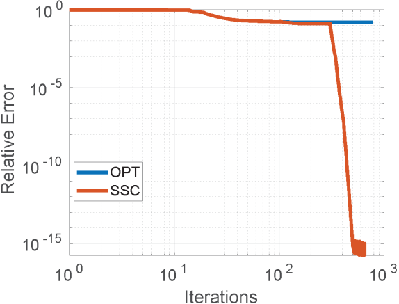
Figure 4: Illustration for performances obtained by OPT in Example 3 for incomplete tensor decomposition. With sensitivity correction, the decomposition can obtain the exact model.

In Appendix I.1, we provide more examples for which the TC algorithms fail to decompose higher-order tensors. Besides high TC-intensity, the sensitivity of the estimated TC model significantly increased, and it prevented the algorithm from converging to the exact model.

3 Sensitivity for TC

We earlier show that any TC model can be unstable since its TC-intensity can grow to infinity. This section introduces the sensitivity of the TC model and its properties.

Definition 3.1 (Sensitivity (SS)).

Given a TC model $\boldsymbol{\mathscr{{Y}}}=\mathopen{{\stackengine{.25ex}{[}{{\scaleto{\circlearrowright}{1.1ex}}}{O}{c}{F}{F}{L}}}\boldsymbol{\mathscr{{A}}}_{1},\dots,\boldsymbol{\mathscr{{A}}}_{N}\mathclose{{\stackengine{.25ex}{]}{\hskip 0.86108pt{\scaleto{\circlearrowleft}{1.1ex}}}{O}{c}{F}{F}{L}}}$. Denote by $\delta_{A_{1}},\dots,\delta_{A_{N}}$ random Gaussian distributed perturbations with element distributed independently with zero mean and variance $\sigma^{2}$. Sensitivity of the TC model $\mathopen{{\stackengine{.25ex}{[}{{\scaleto{\circlearrowright}{1.1ex}}}{O}{c}{F}{F}{L}}}\boldsymbol{\mathscr{{A}}}_{1},\dots,\boldsymbol{\mathscr{{A}}}_{N}\mathclose{{\stackengine{.25ex}{]}{\hskip 0.86108pt{\scaleto{\circlearrowleft}{1.1ex}}}{O}{c}{F}{F}{L}}}$ is defined as

$$ss(\boldsymbol{\mathscr{{A}}}_{1},\dots,\boldsymbol{\mathscr{{A}}}_{N})=\lim_{\sigma^{2}\rightarrow 0}\frac{1}{\sigma^{2}}E\left\{\|\boldsymbol{\mathscr{{Y}}}-\boldsymbol{\mathscr{{Y}}}_{\delta}\|_{F}^{2}\right\},$$ (5)

where $\boldsymbol{\mathscr{{Y}}}_{\delta}=\mathopen{{\stackengine{.25ex}{[}{{\scaleto{\circlearrowright}{1.1ex}}}{O}{c}{F}{F}{L}}}\boldsymbol{\mathscr{{A}}}_{1}+\delta_{A_{1}},\ldots,\boldsymbol{\mathscr{{A}}}_{N}+\delta_{A_{N}}\mathclose{{\stackengine{.25ex}{]}{\hskip 0.86108pt{\scaleto{\circlearrowleft}{1.1ex}}}{O}{c}{F}{F}{L}}}$.

The above sensitivity measure is standard and widely used in the analysis of perturbation of a model or function to the weights e.g., in [37], [38] (Section 2.3.2), [39]. In principle, it measures the mean of the total error variance.

The sensitivity of the function can also be computed as the average Frobenius norm of the Jacobian (or Jacobian norm) as in [40], [41]. The latter definition is approximate of the Frobenius norm of the output difference. Both would lead to a similar compact formula for computing the sensitivity.

We will show that the final expression of the sensitivity is relatively simple and can be written in quadratic forms for each core tensor. It allows us to formulate sub-optimization problems for updating core tensors as constrained quadratic programming that can be solved in closed-form.

Lemma 3.2.

Sensitivity (SS) of a TC model, $\mathopen{{\stackengine{.25ex}{[}{{\scaleto{\circlearrowright}{1.1ex}}}{O}{c}{F}{F}{L}}}\boldsymbol{\mathscr{{A}}}_{1},\dots,\boldsymbol{\mathscr{{A}}}_{N}\mathclose{{\stackengine{.25ex}{]}{\hskip 0.86108pt{\scaleto{\circlearrowleft}{1.1ex}}}{O}{c}{F}{F}{L}}}$, is computed as

$$ss(\boldsymbol{\mathscr{{A}}}_{1},\dots,\boldsymbol{\mathscr{{A}}}_{N})=\sum_{n=1}^{N}I_{n}\,\|\boldsymbol{\mathscr{{A}}}_{-n}\|_{F}^{2}.$$ (6)

where $\boldsymbol{\mathscr{{A}}}_{-n}=\boldsymbol{\mathscr{{A}}}_{n+1}\bullet\cdots\bullet\boldsymbol{\mathscr{{A}}}_{N}\bullet\boldsymbol{\mathscr{{A}}}_{1}\bullet\cdots\bullet\boldsymbol{\mathscr{{A}}}_{n-1}$. Proof is provided in Appendix G.

In principle, TCs with high sensitivity are less stable than those with a smaller SS. A simple normalization that scales the core tensors can reduce the SS.

Lemma 3.3 (Balanced norm for minimal sensitivity).

A TC model $\mathopen{{\stackengine{.25ex}{[}{{\scaleto{\circlearrowright}{1.1ex}}}{O}{c}{F}{F}{L}}}\boldsymbol{\mathscr{{A}}}_{1},\dots,\boldsymbol{\mathscr{{A}}}_{N}\mathclose{{\stackengine{.25ex}{]}{\hskip 0.86108pt{\scaleto{\circlearrowleft}{1.1ex}}}{O}{c}{F}{F}{L}}}$ can be scaled to give a new equivalent model $\mathopen{{\stackengine{.25ex}{[}{{\scaleto{\circlearrowright}{1.1ex}}}{O}{c}{F}{F}{L}}}\boldsymbol{\mathscr{{A}}}_{1},\dots,\boldsymbol{\mathscr{{A}}}_{N}\mathclose{{\stackengine{.25ex}{]}{\hskip 0.86108pt{\scaleto{\circlearrowleft}{1.1ex}}}{O}{c}{F}{F}{L}}}=\mathopen{{\stackengine{.25ex}{[}{{\scaleto{\circlearrowright}{1.1ex}}}{O}{c}{F}{F}{L}}}\alpha_{1}\boldsymbol{\mathscr{{A}}}_{1},\dots,\alpha_{N}\boldsymbol{\mathscr{{A}}}_{N}\mathclose{{\stackengine{.25ex}{]}{\hskip 0.86108pt{\scaleto{\circlearrowleft}{1.1ex}}}{O}{c}{F}{F}{L}}}$ with the minimal sensitivity, where $\alpha_{n}=\frac{\beta_{n}}{\beta}$, $\beta_{n}=\sqrt{I_{n}}\,\|\boldsymbol{\mathscr{{A}}}_{-n}\|_{F}$ and $\beta=\sqrt[N]{\prod_{n=1}^{N}\beta_{n}}$.

Next section presents more efficient algorithms for sensitivity correction.

Remark 3.4.

TC intensity is an upper bound of SS of the model. From SS in (5), we have

$$ss(\mbox{\boldmath$\theta$})\leq\sum_{n=1}^{N}{I_{n}}\,\prod_{k=1,k\neq n}^{N}\|\boldsymbol{\mathscr{{A}}}_{k}\|_{F}^{2}.$$ (7)

where $\theta$ is the vector of parameters.

4 How to deal with Instability in TC- Sensitivity Correction Method

TC’s instability in TC is similar to degeneracy in Canonical Polyadic Decomposition (CPD), which is hard to avoid. We propose to correct the unstable estimated model by seeking a new tensor, $\hat{\boldsymbol{\mathscr{{Y}}}}$, which preserves the approximation error but has smaller sensitivity.

4.1 Rotation method

A simple method is that we scale core tensors following Lemma 3.3. An alternative method is that we rotate two consecutive core tensors by invertible matrices such that the new TC representation has minimum sensitivity

$$\boldsymbol{\mathscr{{Y}}}=\mathopen{{\stackengine{.25ex}{[}{{\scaleto{\circlearrowright}{1.1ex}}}{O}{c}{F}{F}{L}}}{\bf Q}_{3}^{-1}\,\bullet\boldsymbol{\mathscr{{A}}}\bullet{\bf Q}_{1},{\bf Q}_{1}^{-1}\bullet\boldsymbol{\mathscr{{B}}}\bullet{\bf Q}_{2},{\bf Q}_{2}^{-1}\bullet\boldsymbol{\mathscr{{C}}}\bullet{\bf Q}_{3}\mathclose{{\stackengine{.25ex}{]}{\hskip 0.86108pt{\scaleto{\circlearrowleft}{1.1ex}}}{O}{c}{F}{F}{L}}}\,.$$ (8)

For simplicity, we derive the algorithm to find the optimal matrix, ${\bf Q}$ of size $R_{2}\times R_{2}$ which rotates the first two core tensors, $\boldsymbol{\mathscr{{A}}}$ and $\boldsymbol{\mathscr{{B}}}$, and gives a new equivalent TC tensor $\boldsymbol{\mathscr{{Y}}}_{{\bf Q}}=\mathopen{{\stackengine{.25ex}{[}{{\scaleto{\circlearrowright}{1.1ex}}}{O}{c}{F}{F}{L}}}\boldsymbol{\mathscr{{A}}}\bullet{\bf Q},{\bf Q}^{-1}\bullet\boldsymbol{\mathscr{{B}}},\boldsymbol{\mathscr{{C}}}\mathclose{{\stackengine{.25ex}{]}{\hskip 0.86108pt{\scaleto{\circlearrowleft}{1.1ex}}}{O}{c}{F}{F}{L}}}$.

The optimal matrix ${\bf Q}$ which minimizes the sensitivity of $\boldsymbol{\mathscr{{Y}}}_{{\bf Q}}$ is found in the following optimization

$$\min_{{\bf Q}}\;ss(\boldsymbol{\mathscr{{Y}}}_{{\bf Q}})= I_{3}\|\boldsymbol{\mathscr{{A}}}\bullet\boldsymbol{\mathscr{{B}}}\|_{F}^{2}+I_{1}\|{\bf Q}^{-1}\bullet\boldsymbol{\mathscr{{B}}}\bullet\boldsymbol{\mathscr{{C}}}\|_{F}^{2}$$

$$+I_{2}\|{\bf C}\bullet\boldsymbol{\mathscr{{A}}}\bullet{\bf Q}\|_{F}^{2}\,.$$ (9)

We represent the product ${\bf Q}{\bf Q}^{T}={\bf U}{\bf S}{\bf U}^{T}$ in form of EVD, where ${\bf U}$ is an orthogonal matrix of size $R_{2}\times R_{2}$ and ${\bf S}=\operatorname{diag}(s_{1},\ldots,s_{R_{2}})$. Instead of seeking ${\bf Q}$, we find an orthogonal matrix ${\bf U}$ and eigenvalues $s_{r}$.

The optimal eigenvalues are given in closed form as $\displaystyle s_{r}^{\star}=\sqrt{\frac{I_{1}\boldsymbol{u}_{r}^{T}{\bf T}_{1}\boldsymbol{u}_{r}}{I_{2}\boldsymbol{u}_{r}^{T}{\bf T}_{2}\boldsymbol{u}_{r}}}$, for $r=1,\ldots,R_{2}$, where ${\bf T}_{1}=\sum_{i_{2}=1}^{I_{2}}\boldsymbol{\mathscr{{B}}}(:,i_{2},:)({\bf C}_{(1)}{\bf C}_{(1)}^{T})\boldsymbol{\mathscr{{B}}}(:,i_{2},:)^{T}$, and ${\bf T}_{2}=\sum_{i_{1}=1}^{I_{1}}\boldsymbol{\mathscr{{A}}}(:,i_{1},:)^{T}({\bf C}_{(3)}{\bf C}_{(3)}^{T})\boldsymbol{\mathscr{{A}}}(:,i_{1},:)$, ${\bf C}_{(1)}$ and ${\bf C}_{(3)}$ are mode-1 and -$3$ unfoldings of the core tensor $\boldsymbol{\mathscr{{C}}}$. The optimization problem to find the matrix ${\bf U}$ is simplified to

$$\min_{{\bf U}\in St_{R_{2}}}\quad\sum_{r=1}^{R_{2}}\sqrt{(\boldsymbol{u}_{r}^{T}{\bf T}_{1}\boldsymbol{u}_{r})(\boldsymbol{u}_{r}^{T}{\bf T}_{2}\boldsymbol{u}_{r})}\,$$ (10)

and can be solved using the conjugate gradient algorithm on the Stiefel manifold [42]. Algorithm 3 in Appendix summarizes pseudo-codes of the proposed method, which first rotates $\boldsymbol{\mathscr{{A}}}$ and $\boldsymbol{\mathscr{{B}}}$, then performs cyclic-shift of dimensions in the tensor $\boldsymbol{\mathscr{{Y}}}$ to give $\mathopen{{\stackengine{.25ex}{[}{{\scaleto{\circlearrowright}{1.1ex}}}{O}{c}{F}{F}{L}}}\boldsymbol{\mathscr{{A}}},\boldsymbol{\mathscr{{B}}},\boldsymbol{\mathscr{{C}}}\mathclose{{\stackengine{.25ex}{]}{\hskip 0.86108pt{\scaleto{\circlearrowleft}{1.1ex}}}{O}{c}{F}{F}{L}}}=\mathopen{{\stackengine{.25ex}{[}{{\scaleto{\circlearrowright}{1.1ex}}}{O}{c}{F}{F}{L}}}\boldsymbol{\mathscr{{B}}},\boldsymbol{\mathscr{{C}}},\boldsymbol{\mathscr{{A}}}\mathclose{{\stackengine{.25ex}{]}{\hskip 0.86108pt{\scaleto{\circlearrowleft}{1.1ex}}}{O}{c}{F}{F}{L}}}$. A complete derivation of the rotation method for higher order tensors is presented in Appendix F.

4.2 Alternating Sensitivity Correction Method

Both scaling and rotation methods preserve the approximation, transform a TC tensor with high SS to a new equivalent one with a smaller SS. This section proposes another algorithm for sensitivity correction, which updates one core tensor in each iteration. The new algorithm further suppresses the sensitivity to a much lower value. Similar to the rotation method, we formulate the problem of sensitivity correction as minimization of sensitivity with a bound constraint which for order-3 tensor is given by

$$\min\quad ss(\mbox{\boldmath$\theta$})=I_{1}\|\boldsymbol{\mathscr{{B}}}\bullet\boldsymbol{\mathscr{{C}}}\|_{F}^{2}+I_{2}\|\boldsymbol{\mathscr{{C}}}\bullet\boldsymbol{\mathscr{{A}}}\|_{F}^{2}+I_{3}\|\boldsymbol{\mathscr{{A}}}\bullet\boldsymbol{\mathscr{{B}}}\|_{F}^{2}\,$$ (11)

s.t. $$c(\mbox{\boldmath$\theta$})=\|\boldsymbol{\mathscr{{Y}}}-\hat{\boldsymbol{\mathscr{{Y}}}}\|_{F}^{2}\leq\delta^{2},$$

where $\hat{\boldsymbol{\mathscr{{Y}}}}=\mathopen{{\stackengine{.25ex}{[}{{\scaleto{\circlearrowright}{1.1ex}}}{O}{c}{F}{F}{L}}}\boldsymbol{\mathscr{{A}}},\boldsymbol{\mathscr{{B}}},\boldsymbol{\mathscr{{C}}}\mathclose{{\stackengine{.25ex}{]}{\hskip 0.86108pt{\scaleto{\circlearrowleft}{1.1ex}}}{O}{c}{F}{F}{L}}}$. $\delta$ can be the approximation error of the current TC model, i.e., $\delta=\|\boldsymbol{\mathscr{{Y}}}-\hat{\boldsymbol{\mathscr{{Y}}}}_{0}\|_{F}$.

The objective and constraint functions are nonlinear in all core tensors. In order to solve (11), we rewrite the objective function and the constraint function for a single core tensor and solve it using the alternating update scheme. For example, the optimization problem to update the core tensor $\boldsymbol{\mathscr{{A}}}$ is given by

$$\min_{\boldsymbol{\mathscr{{A}}}}\quad ss(\mbox{\boldmath$\theta$})=I_{1}\|\boldsymbol{\mathscr{{B}}}\bullet\boldsymbol{\mathscr{{C}}}\|_{F}^{2}+\mathop{\rm tr}\nolimits({\bf Q}{\bf A}_{(2)}^{T}{\bf A}_{(2)})$$ (12)

s.t. $$\|{\bf Y}_{(1)}-{\bf A}_{(2)}{\bf Z}^{T}\|_{F}^{2}\leq\delta^{2}$$

where ${\bf Q}=I_{2}({\bf I}_{R_{2}}\otimes{\bf C}_{(3)}{\bf C}_{(3)}^{T})+I_{3}({\bf B}_{(1)}{\bf B}_{(1)}^{T}\otimes{\bf I}_{R_{1}})$, ${\bf Z}$ is mode-(1,4) unfolding of the sub-network $\boldsymbol{\mathscr{{B}}}\bullet\boldsymbol{\mathscr{{C}}}$, ${\bf A}_{(2)}$ is mode-2 unfolding of the core tensor $\boldsymbol{\mathscr{{A}}}$, ${\bf Y}_{(1)}$ is mode-1 unfolding of the tensor $\boldsymbol{\mathscr{{Y}}}$. The above optimization problem is quadratic. $\boldsymbol{\mathscr{{A}}}$ can be found in closed form as in Spherical Constrained Quadratic Programming (SCQP) [43, 44, 45].

We summarize pseudo code of the alternating SS correction (SSC) in Algorithm 1. After each update, we perform cyclic shift to the tensor $\boldsymbol{\mathscr{{Y}}}$ and $\hat{\boldsymbol{\mathscr{{Y}}}}$. The order of the TC tensor will be $\mathopen{{\stackengine{.25ex}{[}{{\scaleto{\circlearrowright}{1.1ex}}}{O}{c}{F}{F}{L}}}\boldsymbol{\mathscr{{B}}},\boldsymbol{\mathscr{{C}}},\boldsymbol{\mathscr{{A}}}\mathclose{{\stackengine{.25ex}{]}{\hskip 0.86108pt{\scaleto{\circlearrowleft}{1.1ex}}}{O}{c}{F}{F}{L}}}$. The algorithm for higher-order tensor is presented in Appendix G. A similar algorithm can be applied to correct the TC intensity, where ${\bf Q}$ in (12) is an identity matrix. We often correct intensity before correction of sensitivity.

The entire procedure for efficient TC decomposition with SS control is listed in Algorithm 2. One can start the decomposition with any algorithm in Section 2.1. When SS of the estimated tensor is high exceeds a predefined value, e.g., $10^{7},10^{8}$, the decomposition will converge slowly, and the model tends to be unstable. Algorithm 2 will execute the sensitivity correction in Algorithm 1. The TC decomposition will resume from a new tensor after SSC.

Input: Tensor $\boldsymbol{\mathscr{{Y}}}$: $(I_{1}\times I_{2}\times I_{3})$, and bond dimensions $R$ and error bound $\delta$

Output: $\hat{\boldsymbol{\mathscr{{Y}}}}=\mathopen{{\stackengine{.25ex}{[}{{\scaleto{\circlearrowright}{1.1ex}}}{O}{c}{F}{F}{L}}}\boldsymbol{\mathscr{{A}}},\boldsymbol{\mathscr{{B}}},\boldsymbol{\mathscr{{C}}}\mathclose{{\stackengine{.25ex}{]}{\hskip 0.86108pt{\scaleto{\circlearrowleft}{1.1ex}}}{O}{c}{F}{F}{L}}}$:

$\min ss(\hat{\boldsymbol{\mathscr{{Y}}}})$

s.t.

$\|\boldsymbol{\mathscr{{Y}}}-\hat{\boldsymbol{\mathscr{{Y}}}}\|_{F}^{2}\leq\delta^{2}$

begin

       Initialize $\hat{\boldsymbol{\mathscr{{Y}}}}$

      

      repeat

             Apply balanced normalization, and Rotation method in Algorithm 3

            

            for $n=1,2,3$ do

                   $\boldsymbol{\mathscr{{Z}}}=\boldsymbol{\mathscr{{B}}}\bullet\boldsymbol{\mathscr{{C}}}$

                  

                  ${\bf Q}=I_{2}({\bf I}_{R_{2}}\otimes\boldsymbol{\mathscr{{C}}}_{(3)}\boldsymbol{\mathscr{{C}}}_{(3)}^{T})+I_{3}(\boldsymbol{\mathscr{{B}}}_{(1)}\boldsymbol{\mathscr{{B}}}_{(1)}^{T}\otimes{\bf I}_{R_{1}})$

                  

                  Solve $\boldsymbol{\mathscr{{A}}}=\arg\min_{{\bf X}}\mathop{\rm tr}\nolimits({\bf X}{\bf Q}{\bf X}^{T})\quad\textrm{s.t.}\;\|{\bf Y}_{(1)}-{\bf X}{\bf Z}_{(1,4)}\|_{F}^{2}\leq\delta^{2}$

                  

                  Cyclic-shift of dimensions in $\boldsymbol{\mathscr{{Y}}}$ and $\hat{\boldsymbol{\mathscr{{Y}}}}$

                  

            

      until a stopping criterion is met

Algorithm 1 Sensitivity Correction (SSC)

Input: tensor $\boldsymbol{\mathscr{{Y}}}$: $(I_{1}\times I_{2}\times I_{3})$, and bond dimensions $R$

Output: $\hat{\boldsymbol{\mathscr{{Y}}}}=\mathopen{{\stackengine{.25ex}{[}{{\scaleto{\circlearrowright}{1.1ex}}}{O}{c}{F}{F}{L}}}\boldsymbol{\mathscr{{G}}}_{1},\boldsymbol{\mathscr{{G}}}_{2},\boldsymbol{\mathscr{{G}}}_{3}\mathclose{{\stackengine{.25ex}{]}{\hskip 0.86108pt{\scaleto{\circlearrowleft}{1.1ex}}}{O}{c}{F}{F}{L}}}$

begin

       repeat

             Perform TC decomposition $\hat{\boldsymbol{\mathscr{{Y}}}}$: $\min\;\|\boldsymbol{\mathscr{{Y}}}-\hat{\boldsymbol{\mathscr{{Y}}}}\|_{F}^{2}$

            

            if $ss(\mbox{\boldmath$\theta$})\geq ss_{max}$ then

                   Apply Alg. 1 with $\delta=\|\boldsymbol{\mathscr{{Y}}}-\hat{\boldsymbol{\mathscr{{Y}}}}\|_{F}^{2}$

                  

            

      until a stopping criterion is met

Algorithm 2 TC with SS control (SSCTrl)

5 TC convolutional layer

We apply the proposed algorithms for sensitivity correction in the application for CNN compression. In [46], the authors replace the convolutional kernel and fully connected kernels with the TC model and train the model from scratch. In the case of the pre-trained network given, Aggarwal et al. perform the decomposition of the kernels with parameters randomly generated from a Gaussian distribution. We propose a sequence of 5 layers to replace a convolutional layer. Our method for CNN compression includes the following main steps:

1. Each convolutional kernel is approximated by a tensor decomposition (TC or CPD ).

2. The TC decompositions with diverging components are corrected. The result is a new TC model with minimal sensitivity. CP is also corrected to have minimal sensitivity[44].

3. An initial convolutional kernel is replaced with a tensor in TC or CPD format, which is equivalent to replacing one convolutional layer with a sequence of convolutional layers with a smaller total number of parameters.

4. The entire network is then fine-tuned.

TC Block results in three convolutional layers $W_{1},W_{2},W_{3}$ with shapes ($C_{in}\times R_{1}R_{2}\times 1\times 1$),  3D ($R_{2}\times R_{3}\times 1\times D\times D$) and ($R_{3}R_{1}\times C_{out}\times 1\times 1$), respectively, and two permute/reshape layers $T_{1},T_{2}$ with transform (from $R_{1}R_{2}\times H\times W$ to $R_{2}\times R_{1}\times H\times W$) and (from $R_{3}\times R_{1}\times H\times W$ to $R_{1}R_{3}\times H\times W$), respectively, where $H$ and $W$ are the input dimensions, $R_{1},R_{2},R_{3}$ are TC ranks and $D$ is kernel dimension. Layer order is following: $W_{1},T_{1},W_{2},T_{2},W_{3}$. See Figure 9 in Appendix H).

CPD Block results in three convolutional layers with shapes ($C_{in}\times R\times 1\times 1$), depthwise ($R\times R\times D\times D$) and ($R\times C_{out}\times 1\times 1$), respectively. Here $R$ is CP rank and $D$ is kernel dimension. (See Figure 9 in Appendix H).

Rank Search Procedure. For CP, the smallest rank is chosen such that drop after single layer fine-tuning does not exceed a predefined threshold EPS. TC ranks are selected over the grid with a constraint that the model compressed with TC has fewer FLOPs than the corresponding model compressed with CP.

6 Experiments

Datasets and Computational Resources

We test our algorithms on two representative CNN architectures for image classification: VGG-16 [47], ResNet-18[48]. The networks after fine-tuning are evaluated through top 1 and top 5 accuracy on ILSVRC-12 [49] and CIFAR-10 [50]. The experiments were conducted with the popular neural networks framework Pytorch on a GPU server with NVIDIA V-100 GPUs. As a baseline for CIFAR-10, we used a pre-trained model with 95.17% top-1 accuracy.

For fine-tuning, we used SGD with weight decay of $5\times 10^{-4}$. For the single layer fine-tuning model (Example 7), we fine-tuned the model for 30 epochs with a $10^{-4}$ learning rate. For full model compression (Example 7), models were fine-tuned for 120 epochs by SGD with initial learning rate $10^{-3}$ and decreased every 30 epochs by 10.

Example 4  [Single layer compression in ResNet-18 trained on ILSVRC-12] We decomposed all convolutional kernels except layers 1, 8, and 13 were decomposed using ALS. The ranks-$(R_{1},R_{2},R_{3})$ were chosen to give the number of model parameters close to those in CPD with rank-200. We then applied SSC (Algorithm 1) after 3000 ALS updates. Figure 5(a) compares the relative approximation errors obtained by ALS in 13000 iterations and ALS+SSC. Figure 5(c) illustrates the convergence of the TC decomposition using ALS and ALS+SSC. After the SSC, the decomposition converged to a lower approximation error.

The relative change in approximation error, shown in Figure 5(b), can be 10% for layers 2-6 and smaller for the other layers. We can say that the kernels of convolutional layers 2, 3, …, 7, are well represented by low-rank tensors. Kernels in the last layers have much higher ranks. In our experiment, the approximation error for the last layer was even 0.7489. For this case, SSC is not much helpful.

Figure 5(b) compares the SS of TC models estimated by ALS with and without SSC. The SS was very high for the last layers’ decomposition. The SS grows rapidly to a large number while the approximation error is still high. Approximation of those kernels by a relatively low-rank model will cause degeneracy. Using SSC, we can significantly reduce SS in all decompositions. In summary, SSC will improve the approximation for tensors with good TC approximation and make the decomposition results more stable.

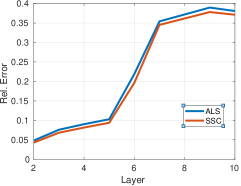
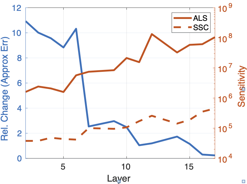
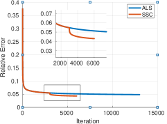
Figure 5: Decomposition of convolutional kernels in ResNet-18 in Example 6. (a) Relative errors obtained by ALS and ALS+SSC, (b) relative changes of the approximation error using SSC, and the SS of estimated tensors, (c) Convergence shown with and without SSC.

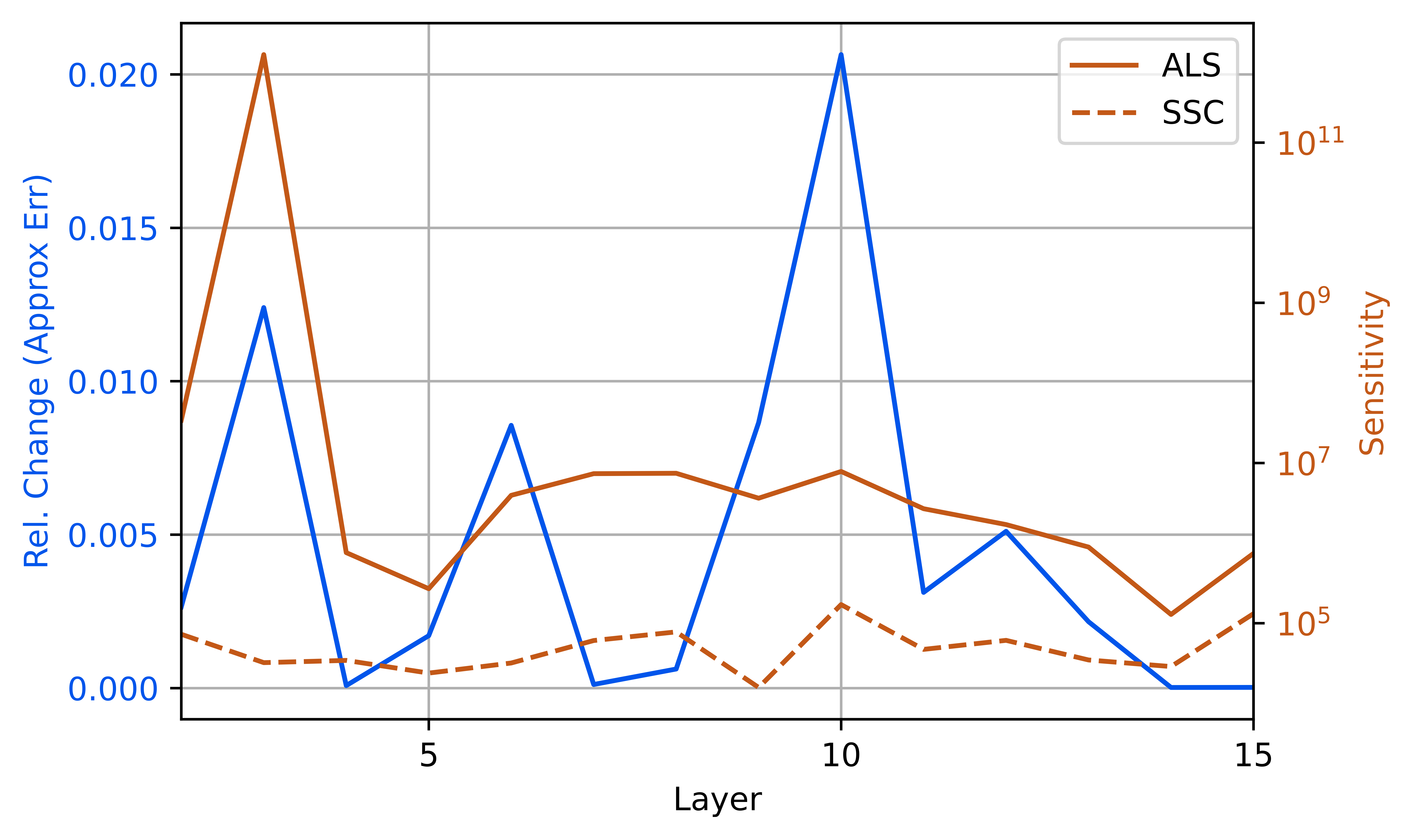
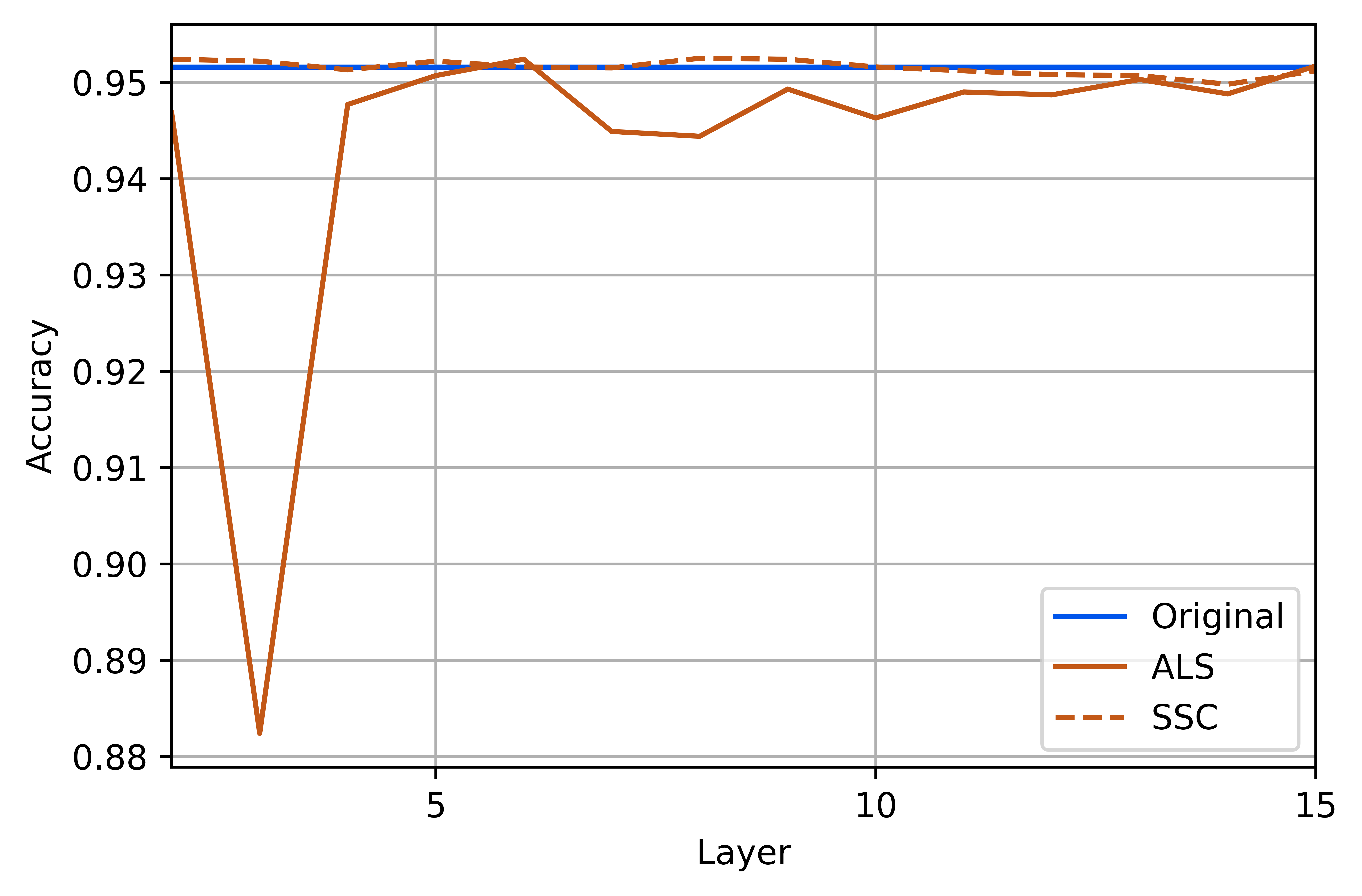
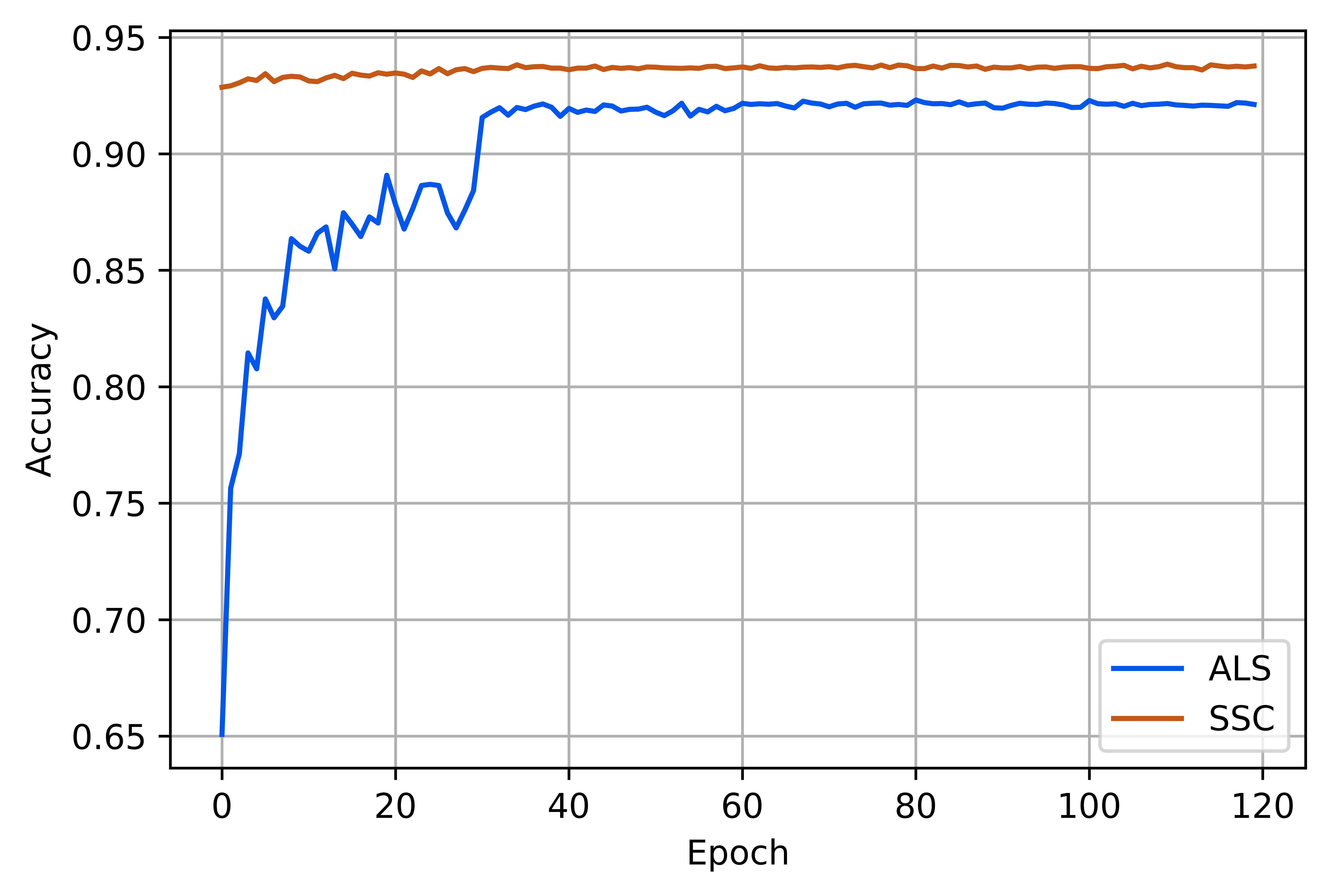
Figure 6: ResNet-18 trained on CIFAR-10. (a) Sensitivity and relative change in approximation error of layers. (b) Accuracy of per layer fine-tuning. (c) Accuracy of full model compression and fine-tuning.

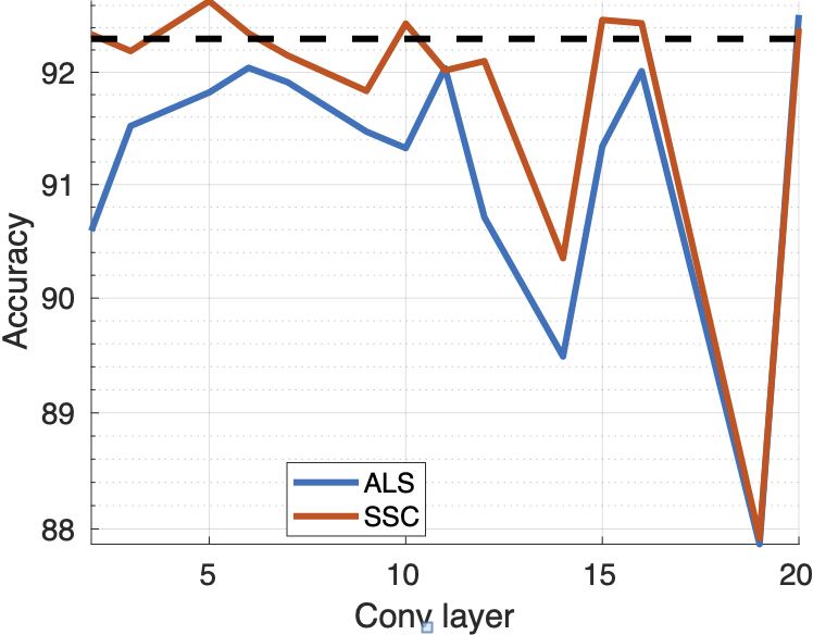
(a) Accuracy

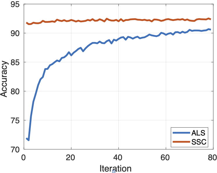
(b) Layer 2

Figure 7: Performance comparison for ALS and (ALS+)SSC in the task for compression of single layers in ResNet-18 finetuned on CIFAR-10. The results are reported for Example 7.

Example 5  [Single layer compression of ResNet-18 on CIFAR-10] We follow the decomposition of kernels in Example 6. The last layer in ResNet-18, trained on ILSVRC-12, is modified and finetuned to work with the CIFAR-10 dataset. Each convolutional layer is replaced with a TC layer presented in Section 5. The new ResNet-18 is finetuned on the CIFAR-10 dataset to update the TC-layer, while the other convolutional layers are frozen. We compared the accuracy of the new type ResNet-18 with TC-layer initialized by the results obtained with ALS and another network initialized by TC tensor obtained with SSC.

The original accuracy of this ResNet-18 for CIFAR-10 is 92.90%. In addition, we do not compress 1x1 convolutional layers, which are layers 8 and 13. TC approximates kernels in layers 2-11 with ranks-(10-10-10), while kernels in layers 12, 14-20 are compressed as in Example 6.

Figure 7 compares accuracy of the two ResNet-18 models. SSC improves the approximation errors and stabilizes the TC network, making the finetuned network attain the best accuracy faster than ResNet-18 using TC with ALS, as seen in Figure 7(b) convergence of the accuracy for the 2nd convolutional layer.

Example 6  [Single layer compression of ResNet-18 on CIFAR-10 with estimation of TC ranks] We train the PyTorch ResNet-18 network adopted for the CIFAR-10 dataset for this experiment. We compute CP ranks for convolutional kernels and TC ranks using the rank selection described in Section 5. SSC gives smaller approximation error and smaller sensitivity than ALS (Figure 6). Each TC layer is finetuned. Figure 6 shows that SSC helps to get better accuracy than ALS.

Example 7  [Full network compression on CIFAR-10] For this experiment we replace all convolutional layers of ResNet-18 except for conv1, layer1.0.conv1 and layer4.1.conv2 by TC layer with ALS and SSC as described in Example 7, remaining convolutional layers are replaced by CPD layers [8]. Figure 6 show that the model with SSC not only converges faster than ALS but also has a significantly higher final accuracy (93.77 % vs. 92.12%).

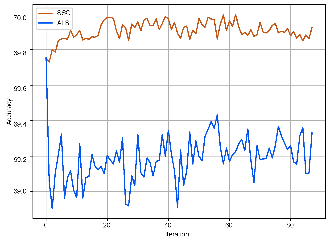
Figure 22: Accuracy vs iteration (one iteration is equal to 500 gradient steps with batch size 256) of single layer fine-tuning for layer4.1.conv2 trained on ILSVRC-12.

Example 8  [Full network compression on ILSVRC-12] We provide extra comparison of full network compression for ResNet-18 and VGG-16 on ILSVRC-12 summarized in Table 1. SSC showed compression results comparable to existing methods. It opens a new direction for combined architectures with CPD-EPC and TC-SSC (See Example 7). In addition, we validate our evaluation of TC-SSC and TC-ALS for single layer fine-tuning on ILSVRC-12 (see Figure 22 in Appendix). Thank to lower sensitivity, TC-SSC exhibits stable convergence to a higher accuracy than TC-ALS.

Table 1: Comparison of different model compression methods on ILSVRC-12 validation dataset.

NN	Method	$\downarrow$ FLOPs	$\downarrow$ Params	$\Delta$ top-1	$\Delta$ top-5
VGG-16	Asym	$\approx 5.00$	-	-	-1.00
	TKD+VBMF	4.93	-	-	-0.50
	CPD-EPC	5.24	1.10	-0.94	-0.33
	SSC[Ours]	5.30	1.10	-6.68	-3.93
	SSC[Ours]	3.76	1.09	-1.47	-0.61
ResNet-18	CG	1.61	-	-1.62	-1.03
	DCP	1.89	-	-2.29	-1.38
	FBS	1.98	-	-2.54	-1.46
	MUSCO	2.42	-	-0.47	-0.30
	CPD-EPC	3.09	3.82	-0.69	-0.15
	SSC[Ours]	3.15	4.05	-1.97	-0.92
	SSC[Ours]	2.49	3.76	-0.86	-0.3

Asym. [51]	TKD+VBMF [14]
DCP [52]	CPD-EPC [8]
FBS [53]	MUSCO [54]
CG [55]

7 Related Works

Since TC was introduced in [16, 17], many algorithms have been developed for various applications, see Section 2.1. However, most studies do not realize the instability problem with TC. The decomposition for incomplete data is even more challenging, as seen in Example 3. No existing algorithm for TC is related to our proposed methods.

Regarding the application for compression of CNN, the authors in [46] encountered the problem of obtaining a good TC decomposition; the authors carefully chose the variance of the initial parameters. However, they were unaware of the numerical instability problem in their decomposition results and did not propose a decomposition method for the TC. Figure 6 in [46] shows that the networks converged slowly and can take 80000 iterations. Slow convergence with the neural network training with ordinary TC layers, i.e., without sensitivity correction, can also be observed in Figure 7(a) and Figure 6 for training ResNet-18 with CIFAR-10 dataset, Figure 22(in Appendix) for ResNet-18 trained on ILSVRC-12 dataset. With Sensitivity Correction, we can train the compressed neural networks quickly and obtain good performances, which are very close to the accuracy of the original neural networks, see, for example, Figure 7(a) and Figure 6. [56] compressed Recurrent Neural Networks with TC layer and implemented the layer as a sum of TT layers. Despite the similarity in applications, the main targets in our work and other studies are different.

8 Conclusions

This paper presents a novel work on the Block term decomposition with shared core tensors (sBTD) and the Tensor Chain. We show that any TC/sBTD model can be unstable with diverging intensity, see Lemma 2.5. We proposed sensitivity for TC as a measure of stability, and confirm the analysis in examples for synthetic data, images, and decomposition of convolutional kernels in ResNet-18. The most important contribution is the novel algorithms that can stabilize the TC/sBTD model and improve the convergence of the decomposition. For compression of CNNs, we proposed a new TC/sBTD layer, which comprises 3 convolutional layers. We show that our proposed methods can help the compressed CNN quickly attain the original accuracy in a few iterations. In contrast, the compressed network cannot be fine-tuned or converge very slowly without sensitivity correction, thereby demanding many iterations.

This supplementary presents proofs of Lemmas introduced in the main manuscript and provides detailed derivation of the Rotation method introduced in Section 4.1 and more illustrative figures for Examples 1-4.

Appendix A Tensor Contraction

Definition A.1 (Tensor train contraction).

performs a tensor contraction between the last mode of $\boldsymbol{\mathscr{{A}}}$ and the first mode of $\boldsymbol{\mathscr{{B}}}$, to yield a tensor $\boldsymbol{\mathscr{{C}}}=\boldsymbol{\mathscr{{A}}}\bullet\boldsymbol{\mathscr{{B}}}$ of size $I_{1}\times\cdots\times I_{N-1}\times J_{2}\times\cdots\times J_{K}$ the elements of which are given by

$$c_{i_{1},\ldots,i_{N-1},j_{2},\ldots,j_{K}}=\sum_{i_{N}=1}^{I_{N}}a_{i_{1},\ldots,i_{N-1},i_{N}}\,b_{i_{N},j_{2},\ldots,j_{K}}.$$

A Tensor train can be expressed as train contraction of core tensors, $\boldsymbol{\mathscr{{X}}}=\boldsymbol{\mathscr{{X}}}_{1}\bullet\boldsymbol{\mathscr{{X}}}_{2}\bullet\cdots\bullet\boldsymbol{\mathscr{{X}}}_{N}$.

Appendix B Proof of Lemma 2.1 (Equivalence of BTD with shared core tensors and TC)

Lemma B.1 (Equivalence of BTD with shared core tensors and TC).

The constrained BTD with shared core tensors in (1) is a Tensor chain model $\boldsymbol{\mathscr{{Y}}}=\mathopen{{\stackengine{.25ex}{[}{{\scaleto{\circlearrowright}{1.1ex}}}{O}{c}{F}{F}{L}}}\boldsymbol{\mathscr{{A}}},\boldsymbol{\mathscr{{B}}},\boldsymbol{\mathscr{{C}}}\mathclose{{\stackengine{.25ex}{]}{\hskip 0.86108pt{\scaleto{\circlearrowleft}{1.1ex}}}{O}{c}{F}{F}{L}}}$ where $\boldsymbol{\mathscr{{A}}}$ is of size $R_{1}\times I_{1}\times R_{2}$ with horizontal slices $\boldsymbol{\mathscr{{A}}}(t,:,:)={\bf A}_{t}$, $\boldsymbol{\mathscr{{C}}}$ of size $R_{3}\times I_{3}\times R_{1}$ and $\boldsymbol{\mathscr{{C}}}(:,:,t)={\bf C}_{t}$, $t=1,\ldots,R_{1}$.

Proof.

∎

The proof is straightforward from the definitions of BTD and TC models

$$\boldsymbol{\mathscr{{Y}}} = \sum_{t=1}^{R_{1}}\sum_{r=1}^{R_{2}}\sum_{s=1}^{R_{3}}{\bf A}_{t}(:,r)\circ\boldsymbol{\mathscr{{B}}}(r,:,s)\circ{\bf C}_{t}(:,s)$$ (13)

$$= \sum_{t=1}^{R_{1}}\sum_{r=1}^{R_{2}}\sum_{s=1}^{R_{3}}\boldsymbol{\mathscr{{A}}}(t,:,r)\circ\boldsymbol{\mathscr{{B}}}(r,:,s)\circ\boldsymbol{\mathscr{{C}}}(s,:,t).$$

Appendix C Proof of Lemma 2 (TC Degeneracy)

Lemma C.1 (TC Degeneracy).

For a given TC model, $\boldsymbol{\mathscr{{Y}}}=\mathopen{{\stackengine{.25ex}{[}{{\scaleto{\circlearrowright}{1.1ex}}}{O}{c}{F}{F}{L}}}\boldsymbol{\mathscr{{A}}},\boldsymbol{\mathscr{{B}}},\boldsymbol{\mathscr{{C}}}\mathclose{{\stackengine{.25ex}{]}{\hskip 0.86108pt{\scaleto{\circlearrowleft}{1.1ex}}}{O}{c}{F}{F}{L}}}$, there is always a sequence of equivalent TC models with diverging TC intensities.

Proof.

∎

We provide an example as proof for the TC model with rank $R_{2}=2$. The other cases can be seen straightforwardly.

Consider the sub-network $\boldsymbol{\mathscr{{A}}}\bullet\boldsymbol{\mathscr{{B}}}$, apply the DMRG-like update rule to split it to a sequence of three cores,

$$\boldsymbol{\mathscr{{A}}}\bullet\boldsymbol{\mathscr{{B}}}=\boldsymbol{\mathscr{{U}}}\bullet{\bf S}\bullet\boldsymbol{\mathscr{{V}}}$$

where ${\bf U}\,{\bf S}\,{\bf V}$ is thin-SVD of unfolding of $\boldsymbol{\mathscr{{A}}}\bullet\boldsymbol{\mathscr{{B}}}$ to a matrix of size $R_{1}I_{1}\times I_{2}R_{3}$, ${\bf S}=\operatorname{diag}(s_{1},s_{2})$ is a diagonal matrix of $R_{2}=2$ leading singular values, ${\bf U}$ and ${\bf V}$ are unfoldings of $\boldsymbol{\mathscr{{U}}}$ and $\boldsymbol{\mathscr{{V}}}$, respectively. The tensor $\boldsymbol{\mathscr{{Y}}}$ has an equivalent TC model $\boldsymbol{\mathscr{{Y}}}=\mathopen{{\stackengine{.25ex}{[}{{\scaleto{\circlearrowright}{1.1ex}}}{O}{c}{F}{F}{L}}}\boldsymbol{\mathscr{{U}}},{\bf S}\bullet\boldsymbol{\mathscr{{V}}},\boldsymbol{\mathscr{{C}}}\mathclose{{\stackengine{.25ex}{]}{\hskip 0.86108pt{\scaleto{\circlearrowleft}{1.1ex}}}{O}{c}{F}{F}{L}}}$.

We next define a matrix ${\bf Q}=\left[\begin{matrix}1&x\\ x&1\end{matrix}\right]$. The tensor $\boldsymbol{\mathscr{{Y}}}$ has another equivalent TC model given by

$$\boldsymbol{\mathscr{{Y}}}=\mathopen{{\stackengine{.25ex}{[}{{\scaleto{\circlearrowright}{1.1ex}}}{O}{c}{F}{F}{L}}}\boldsymbol{\mathscr{{U}}}\bullet{\bf Q},{\bf Q}^{-1}{\bf S}\bullet\boldsymbol{\mathscr{{V}}},\boldsymbol{\mathscr{{C}}}\mathclose{{\stackengine{.25ex}{]}{\hskip 0.86108pt{\scaleto{\circlearrowleft}{1.1ex}}}{O}{c}{F}{F}{L}}}\,$$ (14)

but with an intensity

$$\alpha = \|\boldsymbol{\mathscr{{U}}}\bullet{\bf Q}\|_{F}\,\|{\bf Q}^{-1}{\bf S}\bullet\boldsymbol{\mathscr{{V}}}\|_{F}\,\|\boldsymbol{\mathscr{{C}}}\|_{F}$$ (15)

$$= \|{\bf Q}\|_{F}\,\|{\bf Q}^{-1}{\bf S}\|_{F}\,\|\boldsymbol{\mathscr{{C}}}\|_{F}$$

$$= \frac{(1+x^{2})\sqrt{2(s_{1}^{2}+s_{2}^{2})}}{|1-x^{2}|}\|\boldsymbol{\mathscr{{C}}}\|_{F}\,.$$

It is obvious that when $x$ approaches 1, the intensity $\alpha$ goes to infinity. For the general case, the proof can be derived similarly with a symmetric matrix ${\bf Q}$ of size $R_{2}\times R_{2}$ which has ones on the diagonal and two non-zero off-diagonal elements $x$.

Appendix D Proof of Lemma 3 (Sensitivity for TC)

Proof of Lemma 3 (Sensitivity of TC model).

∎

Consider the error tensor

$$\mathopen{{\stackengine{.25ex}{[}{{\scaleto{\circlearrowright}{1.1ex}}}{O}{c}{F}{F}{L}}}\boldsymbol{\mathscr{{A}}}_{1}+\delta_{\boldsymbol{\mathscr{{A}}}_{1}},\boldsymbol{\mathscr{{A}}}_{2}+\delta_{\boldsymbol{\mathscr{{A}}}_{2}},\ldots,\boldsymbol{\mathscr{{A}}}_{N}+\delta_{\boldsymbol{\mathscr{{A}}}_{N}}\mathclose{{\stackengine{.25ex}{]}{\hskip 0.86108pt{\scaleto{\circlearrowleft}{1.1ex}}}{O}{c}{F}{F}{L}}}-\mathopen{{\stackengine{.25ex}{[}{{\scaleto{\circlearrowright}{1.1ex}}}{O}{c}{F}{F}{L}}}\boldsymbol{\mathscr{{A}}}_{1},\boldsymbol{\mathscr{{A}}}_{2},\ldots,\boldsymbol{\mathscr{{A}}}_{N}\mathclose{{\stackengine{.25ex}{]}{\hskip 0.86108pt{\scaleto{\circlearrowleft}{1.1ex}}}{O}{c}{F}{F}{L}}}$$

$$= \mathopen{{\stackengine{.25ex}{[}{{\scaleto{\circlearrowright}{1.1ex}}}{O}{c}{F}{F}{L}}}\delta_{\boldsymbol{\mathscr{{A}}}_{1}},\boldsymbol{\mathscr{{A}}}_{2},\ldots,\boldsymbol{\mathscr{{A}}}_{N}\mathclose{{\stackengine{.25ex}{]}{\hskip 0.86108pt{\scaleto{\circlearrowleft}{1.1ex}}}{O}{c}{F}{F}{L}}}+\mathopen{{\stackengine{.25ex}{[}{{\scaleto{\circlearrowright}{1.1ex}}}{O}{c}{F}{F}{L}}}{\boldsymbol{\mathscr{{A}}}_{1}},\delta_{\boldsymbol{\mathscr{{A}}}_{2}},\boldsymbol{\mathscr{{A}}}_{3},\ldots,\boldsymbol{\mathscr{{A}}}_{N}\mathclose{{\stackengine{.25ex}{]}{\hskip 0.86108pt{\scaleto{\circlearrowleft}{1.1ex}}}{O}{c}{F}{F}{L}}}+\cdots+\mathopen{{\stackengine{.25ex}{[}{{\scaleto{\circlearrowright}{1.1ex}}}{O}{c}{F}{F}{L}}}{\boldsymbol{\mathscr{{A}}}_{1}},{\boldsymbol{\mathscr{{A}}}_{2}},\ldots,\delta_{\boldsymbol{\mathscr{{A}}}_{N}}\mathclose{{\stackengine{.25ex}{]}{\hskip 0.86108pt{\scaleto{\circlearrowleft}{1.1ex}}}{O}{c}{F}{F}{L}}}+\mathopen{{\stackengine{.25ex}{[}{{\scaleto{\circlearrowright}{1.1ex}}}{O}{c}{F}{F}{L}}}\delta_{\boldsymbol{\mathscr{{A}}}_{1}},\delta_{\boldsymbol{\mathscr{{A}}}_{2}},{\boldsymbol{\mathscr{{A}}}_{3}},\ldots,{\boldsymbol{\mathscr{{A}}}_{N}}\mathclose{{\stackengine{.25ex}{]}{\hskip 0.86108pt{\scaleto{\circlearrowleft}{1.1ex}}}{O}{c}{F}{F}{L}}}$$

$$+\mathopen{{\stackengine{.25ex}{[}{{\scaleto{\circlearrowright}{1.1ex}}}{O}{c}{F}{F}{L}}}\delta_{\boldsymbol{\mathscr{{A}}}_{1}},{\boldsymbol{\mathscr{{A}}}_{2}},\ldots,\delta_{\boldsymbol{\mathscr{{A}}}_{N}}\mathclose{{\stackengine{.25ex}{]}{\hskip 0.86108pt{\scaleto{\circlearrowleft}{1.1ex}}}{O}{c}{F}{F}{L}}}+\cdots+\mathopen{{\stackengine{.25ex}{[}{{\scaleto{\circlearrowright}{1.1ex}}}{O}{c}{F}{F}{L}}}\delta_{\boldsymbol{\mathscr{{A}}}_{1}},\delta_{\boldsymbol{\mathscr{{A}}}_{2}},\ldots,\delta_{\boldsymbol{\mathscr{{A}}}_{N}}\mathclose{{\stackengine{.25ex}{]}{\hskip 0.86108pt{\scaleto{\circlearrowleft}{1.1ex}}}{O}{c}{F}{F}{L}}}.$$

TC terms in the above expression are uncorrelated, and the expectation of the terms consisting of two or more $\delta_{\boldsymbol{\mathscr{{A}}}_{n}}$ is zero. Hence, the expectation in (5) is rewritten as

$$E\{\|\boldsymbol{\mathscr{{Y}}}-\mathopen{{\stackengine{.25ex}{[}{{\scaleto{\circlearrowright}{1.1ex}}}{O}{c}{F}{F}{L}}}\boldsymbol{\mathscr{{A}}}_{1}+\delta_{\boldsymbol{\mathscr{{A}}}_{1}},\boldsymbol{\mathscr{{A}}}_{2}+\delta_{\boldsymbol{\mathscr{{A}}}_{2}},\ldots,\boldsymbol{\mathscr{{A}}}_{N}+\delta_{\boldsymbol{\mathscr{{A}}}_{N}}\mathclose{{\stackengine{.25ex}{]}{\hskip 0.86108pt{\scaleto{\circlearrowleft}{1.1ex}}}{O}{c}{F}{F}{L}}}\|_{F}^{2}\}$$

$$=E\{\|\mathopen{{\stackengine{.25ex}{[}{{\scaleto{\circlearrowright}{1.1ex}}}{O}{c}{F}{F}{L}}}\delta_{\boldsymbol{\mathscr{{A}}}_{1}},\boldsymbol{\mathscr{{A}}}_{2},\ldots,\boldsymbol{\mathscr{{A}}}_{N}\mathclose{{\stackengine{.25ex}{]}{\hskip 0.86108pt{\scaleto{\circlearrowleft}{1.1ex}}}{O}{c}{F}{F}{L}}}\|_{F}^{2}\}+E\{\|\mathopen{{\stackengine{.25ex}{[}{{\scaleto{\circlearrowright}{1.1ex}}}{O}{c}{F}{F}{L}}}{\boldsymbol{\mathscr{{A}}}_{1}},\delta_{\boldsymbol{\mathscr{{A}}}_{2}},\boldsymbol{\mathscr{{A}}}_{3},\ldots,\boldsymbol{\mathscr{{A}}}_{N}\mathclose{{\stackengine{.25ex}{]}{\hskip 0.86108pt{\scaleto{\circlearrowleft}{1.1ex}}}{O}{c}{F}{F}{L}}}\|_{F}^{2}\}+\cdots+E\{\|\mathopen{{\stackengine{.25ex}{[}{{\scaleto{\circlearrowright}{1.1ex}}}{O}{c}{F}{F}{L}}}{\boldsymbol{\mathscr{{A}}}_{1}},{\boldsymbol{\mathscr{{A}}}_{2}},\ldots,\delta_{\boldsymbol{\mathscr{{A}}}_{N}}\mathclose{{\stackengine{.25ex}{]}{\hskip 0.86108pt{\scaleto{\circlearrowleft}{1.1ex}}}{O}{c}{F}{F}{L}}}\|_{F}^{2}\}\,$$

$$=E\{\|\mathopen{{\stackengine{.25ex}{[}{{\scaleto{\circlearrowright}{1.1ex}}}{O}{c}{F}{F}{L}}}\delta_{\boldsymbol{\mathscr{{A}}}_{1}},\boldsymbol{\mathscr{{A}}}_{-1}\mathclose{{\stackengine{.25ex}{]}{\hskip 0.86108pt{\scaleto{\circlearrowleft}{1.1ex}}}{O}{c}{F}{F}{L}}}\|_{F}^{2}\}+E\{\|\mathopen{{\stackengine{.25ex}{[}{{\scaleto{\circlearrowright}{1.1ex}}}{O}{c}{F}{F}{L}}}\delta_{\boldsymbol{\mathscr{{A}}}_{2}},\boldsymbol{\mathscr{{A}}}_{-2}\mathclose{{\stackengine{.25ex}{]}{\hskip 0.86108pt{\scaleto{\circlearrowleft}{1.1ex}}}{O}{c}{F}{F}{L}}}\|_{F}^{2}\}+\cdots+E\{\|\mathopen{{\stackengine{.25ex}{[}{{\scaleto{\circlearrowright}{1.1ex}}}{O}{c}{F}{F}{L}}}\delta_{\boldsymbol{\mathscr{{A}}}_{N}},\boldsymbol{\mathscr{{A}}}_{-N}\mathclose{{\stackengine{.25ex}{]}{\hskip 0.86108pt{\scaleto{\circlearrowleft}{1.1ex}}}{O}{c}{F}{F}{L}}}\|_{F}^{2}\}.$$ (16)

Thank to looping structure of the TC tensor, we can cyclic shift $\delta_{\boldsymbol{\mathscr{{A}}}_{n}}$ to the first core tensor, and the rest part of the tensor is the TT-tensor $\boldsymbol{\mathscr{{A}}}_{-n}$.

We reshape the TC tensor, $\mathopen{{\stackengine{.25ex}{[}{{\scaleto{\circlearrowright}{1.1ex}}}{O}{c}{F}{F}{L}}}\delta_{\boldsymbol{\mathscr{{A}}}_{n}},\boldsymbol{\mathscr{{A}}}_{-n}\mathclose{{\stackengine{.25ex}{]}{\hskip 0.86108pt{\scaleto{\circlearrowleft}{1.1ex}}}{O}{c}{F}{F}{L}}}$, to mode-1 unfolding and expand its Frobenius norm as

$$E\{\|\mathopen{{\stackengine{.25ex}{[}{{\scaleto{\circlearrowright}{1.1ex}}}{O}{c}{F}{F}{L}}}\delta_{\boldsymbol{\mathscr{{A}}}_{1}},\boldsymbol{\mathscr{{A}}}_{-1}\mathclose{{\stackengine{.25ex}{]}{\hskip 0.86108pt{\scaleto{\circlearrowleft}{1.1ex}}}{O}{c}{F}{F}{L}}}\|_{F}^{2}\} = E\{\|[\delta_{\boldsymbol{\mathscr{{A}}}_{1}}]_{(2)}[\boldsymbol{\mathscr{{A}}}_{-1}]_{(1,N)}\|_{F}^{2}\}$$

$$= E\{\mathop{\rm tr}\nolimits([\delta_{\boldsymbol{\mathscr{{A}}}_{1}}]_{(2)}^{T}[\delta_{\boldsymbol{\mathscr{{A}}}_{1}}]_{(2)})([\boldsymbol{\mathscr{{A}}}_{-1}]_{(1,N)}[\boldsymbol{\mathscr{{A}}}_{-1}]_{(1,N)}^{T}))\}=\sigma^{2}I_{1}\mathop{\rm tr}\nolimits([\boldsymbol{\mathscr{{A}}}_{-1}]_{(1,N)}[\boldsymbol{\mathscr{{A}}}_{-1}]_{(1,N)}^{T}))$$

$$= \sigma^{2}I_{1}\|\boldsymbol{\mathscr{{A}}}_{-1}\|_{F}^{2}.$$

Together with (16), we finally complete the proof.

Appendix E Proof of Lemma 4 (Balanced norm for minimal sensitivity)

Proof.

Since $\alpha_{1}\alpha_{2}\cdots\alpha_{N}=1$, we have two equivalent TC models $\mathopen{{\stackengine{.25ex}{[}{{\scaleto{\circlearrowright}{1.1ex}}}{O}{c}{F}{F}{L}}}\boldsymbol{\mathscr{{A}}}_{1},\boldsymbol{\mathscr{{A}}}_{2},\ldots,\boldsymbol{\mathscr{{A}}}_{N}\mathclose{{\stackengine{.25ex}{]}{\hskip 0.86108pt{\scaleto{\circlearrowleft}{1.1ex}}}{O}{c}{F}{F}{L}}}=\mathopen{{\stackengine{.25ex}{[}{{\scaleto{\circlearrowright}{1.1ex}}}{O}{c}{F}{F}{L}}}\alpha_{1}\boldsymbol{\mathscr{{A}}}_{1},\alpha_{2}\boldsymbol{\mathscr{{A}}}_{2},\ldots,\alpha_{N}\boldsymbol{\mathscr{{A}}}_{N}\mathclose{{\stackengine{.25ex}{]}{\hskip 0.86108pt{\scaleto{\circlearrowleft}{1.1ex}}}{O}{c}{F}{F}{L}}}$. Sensitivity of the new model is given by

$$ss(\mathopen{{\stackengine{.25ex}{[}{{\scaleto{\circlearrowright}{1.1ex}}}{O}{c}{F}{F}{L}}}\alpha_{1}\boldsymbol{\mathscr{{A}}}_{1},\alpha_{2}\boldsymbol{\mathscr{{A}}}_{2},\ldots,\alpha_{N}\boldsymbol{\mathscr{{A}}}_{N}\mathclose{{\stackengine{.25ex}{]}{\hskip 0.86108pt{\scaleto{\circlearrowleft}{1.1ex}}}{O}{c}{F}{F}{L}}}) = \sum_{n=1}^{N}I_{n}\left(\prod_{k\neq n}\alpha_{k}^{2}\right)\,\|\boldsymbol{\mathscr{{A}}}_{-n}\|_{F}^{2}$$

$$= \sum_{n=1}^{N}\frac{\beta_{n}^{2}}{\alpha_{n}^{2}}$$

$$\geq N\sqrt[N]{\frac{\beta_{1}^{2}\,\beta_{2}^{2}\,\cdots\beta_{N}^{2}}{\alpha_{1}^{2}\alpha_{2}^{2}\cdots\alpha_{N}^{2}}}=N\beta^{2}\,.$$

The inequality is between the arithmetic mean and the geometric mean, and the equality in it holds when all terms are equal each to the other, i.e.,

$$\frac{\beta_{1}}{\alpha_{1}}=\frac{\beta_{2}}{\alpha_{2}}=\cdots=\frac{\beta_{N}}{\alpha_{N}}=\sqrt[N]{\frac{\beta_{1}\,\beta_{2}\cdots\,\beta_{N}}{\alpha_{1}\,\alpha_{2}\,\cdots\alpha_{N}}}=\beta\,.$$ (17)

Hence $\alpha_{n}=\frac{\beta_{n}}{\beta}$. This completes the proof. ∎

Appendix F Rotation method for Sensitivity Correction

This section presents the complete derivation of the Rotation algorithm in Section 4.1. Due to space limitations, we present a brief derivation of the Rotation method in the main manuscript.

Due to non uniqueness of the model up to rotation, we can rotate core tensors by invertible matrices such that the new representation of the TC tensor has minimum sensitivity

$$\boldsymbol{\mathscr{{Y}}}=\mathopen{{\stackengine{.25ex}{[}{{\scaleto{\circlearrowright}{1.1ex}}}{O}{c}{F}{F}{L}}}{\bf Q}_{N}^{-1}\,\bullet\boldsymbol{\mathscr{{A}}}_{1}\bullet{\bf Q}_{1},{\bf Q}_{1}^{-1}\bullet\boldsymbol{\mathscr{{A}}}_{2}\bullet{\bf Q}_{2},{\bf Q}_{2}^{-1}\bullet\boldsymbol{\mathscr{{A}}}_{3}\bullet{\bf Q}_{3},\ldots,{\bf Q}_{N-1}^{-1}\boldsymbol{\mathscr{{A}}}_{N}{\bf Q}_{N}\mathclose{{\stackengine{.25ex}{]}{\hskip 0.86108pt{\scaleto{\circlearrowleft}{1.1ex}}}{O}{c}{F}{F}{L}}}\,.$$ (18)

For simplicity, we derive the algorithm to find the optimal matrix, ${\bf Q}$ of size $R_{2}\times R_{2}$ which rotates the first two core tensors, $\boldsymbol{\mathscr{{A}}}_{1}$ and $\boldsymbol{\mathscr{{A}}}_{2}$, and gives a new equivalent TC tensor $\boldsymbol{\mathscr{{Y}}}_{{\bf Q}}=\mathopen{{\stackengine{.25ex}{[}{{\scaleto{\circlearrowright}{1.1ex}}}{O}{c}{F}{F}{L}}}\boldsymbol{\mathscr{{A}}}_{1}\bullet{\bf Q},{\bf Q}^{-1}\bullet\boldsymbol{\mathscr{{A}}}_{2},\boldsymbol{\mathscr{{A}}}_{3},\ldots,\boldsymbol{\mathscr{{A}}}_{N}\mathclose{{\stackengine{.25ex}{]}{\hskip 0.86108pt{\scaleto{\circlearrowleft}{1.1ex}}}{O}{c}{F}{F}{L}}}$.

The optimal matrix ${\bf Q}$ minimizes the sensitivity of $\boldsymbol{\mathscr{{Y}}}_{{\bf Q}}$

$$\min_{{\bf Q}}\quad ss(\boldsymbol{\mathscr{{Y}}}_{{\bf Q}})=I_{1}\|{\bf Q}^{-1}\boldsymbol{\mathscr{{A}}}_{-1}\|_{F}^{2}+I_{2}\|\boldsymbol{\mathscr{{A}}}_{-2}{\bf Q}\|_{F}^{2}+\sum_{n=3}^{N}I_{n}\|\boldsymbol{\mathscr{{A}}}_{-n}\|_{F}^{2}\,$$ (19)

where $\boldsymbol{\mathscr{{A}}}_{-n}=\boldsymbol{\mathscr{{A}}}_{n+1}\bullet\cdots\bullet\boldsymbol{\mathscr{{A}}}_{N}\bullet\boldsymbol{\mathscr{{A}}}_{1}\bullet\cdots\bullet\boldsymbol{\mathscr{{A}}}_{n-1}$.

We next define two matrices, ${\bf X}_{1}$ of size $R_{3}\times R_{3}$ and ${\bf X}_{2}$ of size $R_{1}\times R_{1}$, as self contraction of the tensor $\boldsymbol{\mathscr{{A}}}_{-(1,2)}=\boldsymbol{\mathscr{{A}}}_{3}\bullet\cdots\bullet\boldsymbol{\mathscr{{A}}}_{N}$ along all modes but mode-1 and mode-$N$, respectively

$${\bf X}_{1}=[\boldsymbol{\mathscr{{A}}}_{-(1,2)}]_{(1)}[\boldsymbol{\mathscr{{A}}}_{-(1,2)}]_{(1)}^{T}\,,\quad{\bf X}_{2}=[\boldsymbol{\mathscr{{A}}}_{-(1,2)}]_{(N)}[\boldsymbol{\mathscr{{A}}}_{-(1,2)}]_{(N)}^{T}\quad$$ (20)

and two square matrices, ${\bf T}_{1}$ and ${\bf T}_{2}$, of size $R_{2}\times R_{2}$

$${\bf T}_{1} = \sum_{i_{2}=1}^{I_{2}}\boldsymbol{\mathscr{{A}}}_{2}(:,i_{2},:){\bf X}_{1}\boldsymbol{\mathscr{{A}}}_{2}(:,i_{2},:)^{T},\qquad\quad{\bf T}_{2}=\sum_{i_{1}=1}^{I_{1}}\boldsymbol{\mathscr{{A}}}_{1}(:,i_{1},:)^{T}{\bf X}_{2}\boldsymbol{\mathscr{{A}}}_{1}(:,i_{1},:)\,.$$ (21)

See illustration for efficient computation of ${\bf X}_{1}$ and ${\bf X}_{2}$ in Figure 8.

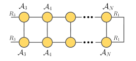
(a) ${\bf X}_{1}$: self-contraction of the TT-tensor, $\boldsymbol{\mathscr{{A}}}_{3:N}$, along modes-$2,3,\ldots,N$

(b) ${\bf X}_{2}$: self-contraction of the TT-tensor, $\boldsymbol{\mathscr{{A}}}_{3:N}$, along modes-$1,3,\ldots,N-1$

Figure 8: Computation of ${\bf X}_{1}$ and ${\bf X}_{2}$ as self-contraction of the tensor $\boldsymbol{\mathscr{{A}}}_{-(1,2)}=\boldsymbol{\mathscr{{A}}}_{3:N}=\boldsymbol{\mathscr{{A}}}_{3}\bullet\boldsymbol{\mathscr{{A}}}_{4}\bullet\cdots\bullet\boldsymbol{\mathscr{{A}}}_{N}$. For efficient computation, we can compute self-contraction of core tensors $\boldsymbol{\mathscr{{A}}}_{3}$, $\boldsymbol{\mathscr{{A}}}_{4}$, …, $\boldsymbol{\mathscr{{A}}}_{N}$ along their second modes to give matrices, ${\bf B}_{n}=\sum_{i=1}^{I_{n}}\boldsymbol{\mathscr{{A}}}_{n}(:,i,:)\otimes\boldsymbol{\mathscr{{A}}}_{n}(:,i,:)$ of size $R_{n}^{2}\times R_{n+1}^{2}$. Then ${\bf X}_{1}$ is given by $\operatorname{vec}\left({\bf X}_{1}\right)={\bf B}_{3}\cdots{\bf B}_{N-1}{\bf B}_{N}\mbox{\boldmath$1$}$ and $\operatorname{vec}\left({\bf X}_{2}\right)={\bf B}_{N}^{T}{\bf B}_{N-1}^{T}\cdots{\bf B}_{4}^{T}{\bf B}_{3}^{T}\mbox{\boldmath$1$}$.

We represent the matrix ${\bf Q}{\bf Q}^{T}={\bf U}{\bf S}{\bf U}^{T}$ in form of its eigenvalue decomposition (EVD), where ${\bf U}$ is an orthogonal matrix of size $R_{2}\times R_{2}$ and ${\bf S}=\operatorname{diag}(s_{1},\ldots,s_{R_{2}})$. The sensitivity in (19) is then computed as

$$ss(\boldsymbol{\mathscr{{Y}}}_{{\bf Q}}) = I_{1}\|{\bf Q}^{-1}\boldsymbol{\mathscr{{A}}}_{-1}\|_{F}^{2}+I_{2}\|\boldsymbol{\mathscr{{A}}}_{-2}{\bf Q}\|_{F}^{2}+\sum_{n=3}^{N}I_{n}\|\boldsymbol{\mathscr{{A}}}_{-n}\|_{F}^{2}$$

$$= \sum_{n=3}^{N}I_{n}\|\boldsymbol{\mathscr{{A}}}_{-n}\|_{F}^{2}+I_{1}\mathop{\rm tr}\nolimits({\bf T}_{1}{\bf Q}^{-1}{\bf Q}^{-1T})+I_{2}\mathop{\rm tr}\nolimits({\bf T}_{2}{\bf Q}{\bf Q}^{T})$$

$$= \sum_{n=3}^{N}I_{n}\|\boldsymbol{\mathscr{{A}}}_{-n}\|_{F}^{2}+I_{1}\mathop{\rm tr}\nolimits(({\bf U}^{T}{\bf T}_{1}{\bf U}){\bf S}^{-1})+I_{2}\mathop{\rm tr}\nolimits(({\bf U}^{T}{\bf T}_{2}{\bf U}){\bf S}).$$

Instead of seeking ${\bf Q}$, we find an orthogonal matrix ${\bf U}$ and a diagonal matrix ${\bf S}$

$$ss(\boldsymbol{\mathscr{{Y}}}_{{\bf Q}})=\sum_{n=3}^{N}I_{n}\|\boldsymbol{\mathscr{{A}}}_{-n}\|_{F}^{2}+\sum_{r=1}^{R_{2}}I_{1}(\boldsymbol{u}_{r}^{T}{\bf T}_{1}\boldsymbol{u}_{r})\frac{1}{s_{r}}+I_{2}(\boldsymbol{u}_{r}^{T}{\bf T}_{2}\boldsymbol{u}_{r})s_{r}$$

$$\geq\sum_{n=3}^{N}I_{n}\|\boldsymbol{\mathscr{{A}}}_{-n}\|_{F}^{2}+\sum_{r=1}^{R_{2}}2\sqrt{I_{1}I_{2}(\boldsymbol{u}_{r}^{T}{\bf T}_{1}\boldsymbol{u}_{r})(\boldsymbol{u}_{r}^{T}{\bf T}_{2}\boldsymbol{u}_{r})}\,.$$ (22)

The equality holds when

$$\displaystyle s_{r}^{\star}=\sqrt{\frac{I_{1}\boldsymbol{u}_{r}^{T}{\bf T}_{1}\boldsymbol{u}_{r}}{I_{2}\boldsymbol{u}_{r}^{T}{\bf T}_{2}\boldsymbol{u}_{r}}}$$ (23)

for $r=1,\ldots,R_{2}$. Given the optimal $s_{r}^{\star}$, we find the orthogonal matrix ${\bf U}$ in the following optimization problem

$$\min_{{\bf U}\in St_{R_{2}}}\quad\sum_{r=1}^{R_{2}}\sqrt{(\boldsymbol{u}_{r}^{T}{\bf T}_{1}\boldsymbol{u}_{r})(\boldsymbol{u}_{r}^{T}{\bf T}_{2}\boldsymbol{u}_{r})}\,,$$ (24)

which can be solved using the conjugate gradient algorithm on the Stiefel manifold [42].

Initialization. Applying the Cauchy-Schwarz inequality, the objective function in (10) is bounded above by $\frac{1}{2}\sum_{r=1}^{R_{2}}(\boldsymbol{u}_{r}^{T}{\bf T}_{1}\boldsymbol{u}_{r})+(\boldsymbol{u}_{r}^{T}{\bf T}_{2}\boldsymbol{u}_{r})=\frac{1}{2}\mathop{\rm tr}\nolimits({\bf U}^{T}({\bf T}_{1}+{\bf T}_{2}){\bf U})$. We can initialize ${\bf U}$ by eigenvectors of $({\bf T}_{1}+{\bf T}_{2})$.

The rotation method is then applied to the next pair $\boldsymbol{\mathscr{{A}}}_{2}$ and $\boldsymbol{\mathscr{{A}}}_{3}$, $\boldsymbol{\mathscr{{A}}}_{3}$ and $\boldsymbol{\mathscr{{A}}}_{4}$, …, $\boldsymbol{\mathscr{{A}}}_{N}$ and $\boldsymbol{\mathscr{{A}}}_{1}$, …until the update reaches a stopping criterion. Pseudo-codes of the proposed algorithm for order-3 TC are listed in Algorithm 3.

Input: TC tensor $\boldsymbol{\mathscr{{Y}}}=\mathopen{{\stackengine{.25ex}{[}{{\scaleto{\circlearrowright}{1.1ex}}}{O}{c}{F}{F}{L}}}\boldsymbol{\mathscr{{A}}},\boldsymbol{\mathscr{{B}}},\boldsymbol{\mathscr{{C}}}\mathclose{{\stackengine{.25ex}{]}{\hskip 0.86108pt{\scaleto{\circlearrowleft}{1.1ex}}}{O}{c}{F}{F}{L}}}$: $(I_{1}\times I_{2}\times I_{3})$, and bond dimensions $R$

Output: $\hat{\boldsymbol{\mathscr{{Y}}}}=\boldsymbol{\mathscr{{Y}}}$ such that $\min\quad ss(\hat{\boldsymbol{\mathscr{{Y}}}})$

begin

       repeat

             for $n=1,2,3$ do

                   ${\bf T}_{1}=\sum_{i_{2}=1}^{I_{2}}{\bf B}_{i_{2}}({\bf C}_{(1)}{\bf C}_{(1)}^{T}){\bf B}_{i_{2}}^{T}$,

                   ${\bf T}_{2}=\sum_{i_{1}=1}^{I_{1}}{\bf A}_{i_{1}}^{T}({\bf C}_{(3)}{\bf C}_{(3)}^{T}){\bf A}_{i_{1}}$

                  

                  Solve ${\bf U}^{*}=\arg\min_{{\bf U}\in St_{R_{2}}}\quad\sum_{r=1}^{R_{2}}\sqrt{(\boldsymbol{u}_{r}^{T}{\bf T}_{1}\boldsymbol{u}_{r})(\boldsymbol{u}_{r}^{T}{\bf T}_{2}\boldsymbol{u}_{r})}$

                  

                  for $r=1\ldots,R_{2}$ do  $\displaystyle s_{r}^{\star}=\sqrt{\frac{I_{1}\boldsymbol{u}_{r}^{T}{\bf T}_{1}\boldsymbol{u}_{r}}{I_{2}\boldsymbol{u}_{r}^{T}{\bf T}_{2}\boldsymbol{u}_{r}}}$

                  

                  Rotate $\boldsymbol{\mathscr{{A}}}\leftarrow\boldsymbol{\mathscr{{A}}}\bullet{\bf U}\operatorname{diag}(\sqrt{s_{1}},\ldots,\sqrt{s_{R_{2}}},\ldots){\bf U}^{T}$

                  Rotate $\boldsymbol{\mathscr{{B}}}\leftarrow{\bf U}\operatorname{diag}(1/\sqrt{s_{1}},\ldots,1/\sqrt{s_{R_{2}}},\ldots){\bf U}^{T}\bullet\boldsymbol{\mathscr{{B}}}$

                  Cyclic-shift of dimensions $\hat{\boldsymbol{\mathscr{{Y}}}}=\mathopen{{\stackengine{.25ex}{[}{{\scaleto{\circlearrowright}{1.1ex}}}{O}{c}{F}{F}{L}}}\boldsymbol{\mathscr{{A}}},\boldsymbol{\mathscr{{B}}},\boldsymbol{\mathscr{{C}}}\mathclose{{\stackengine{.25ex}{]}{\hskip 0.86108pt{\scaleto{\circlearrowleft}{1.1ex}}}{O}{c}{F}{F}{L}}}\leftarrow\mathopen{{\stackengine{.25ex}{[}{{\scaleto{\circlearrowright}{1.1ex}}}{O}{c}{F}{F}{L}}}\boldsymbol{\mathscr{{B}}},\boldsymbol{\mathscr{{C}}},\boldsymbol{\mathscr{{A}}}\mathclose{{\stackengine{.25ex}{]}{\hskip 0.86108pt{\scaleto{\circlearrowleft}{1.1ex}}}{O}{c}{F}{F}{L}}}$

                  

            

      until a stopping criterion is met

Algorithm 3 Rotation Method for SSC

Appendix G Sensitivity Correction for Higher Order TC

The optimization problem for Sensitivity correction for higher order TC is formulated in a similar form for TC of order-3, i.e., minimizing the SS of the model while keeping the approximation error bounded

$$\min\quad ss(\mbox{\boldmath$\theta$})=\sum_{n}I_{n}\|\boldsymbol{\mathscr{{A}}}_{-n}\|_{F}^{2}\,$$ (25)

s.t. $$c(\mbox{\boldmath$\theta$})=\|\boldsymbol{\mathscr{{Y}}}-\hat{\boldsymbol{\mathscr{{Y}}}}\|_{F}^{2}\leq\delta^{2},$$

where $\hat{\boldsymbol{\mathscr{{Y}}}}=\mathopen{{\stackengine{.25ex}{[}{{\scaleto{\circlearrowright}{1.1ex}}}{O}{c}{F}{F}{L}}}\boldsymbol{\mathscr{{A}}}_{1},\boldsymbol{\mathscr{{A}}}_{2},\ldots,\boldsymbol{\mathscr{{A}}}_{N}\mathclose{{\stackengine{.25ex}{]}{\hskip 0.86108pt{\scaleto{\circlearrowleft}{1.1ex}}}{O}{c}{F}{F}{L}}}$ and $\delta$ can be the approximation error of the current TC model, i.e., $\delta=\|\boldsymbol{\mathscr{{Y}}}-\hat{\boldsymbol{\mathscr{{Y}}}}_{0}\|_{F}$.

In order to update $\boldsymbol{\mathscr{{A}}}_{1}$, we rewrite the sensitivity function as function of the core tensor $\boldsymbol{\mathscr{{A}}}_{1}$

$$ss(\mbox{\boldmath$\theta$}) =I_{1}\|\boldsymbol{\mathscr{{A}}}_{-1}\|_{F}^{2}+\sum_{n=2}^{N}I_{n}\|\boldsymbol{\mathscr{{A}}}_{-n}\|_{F}^{2}$$

$$=I_{1}\|\boldsymbol{\mathscr{{A}}}_{-1}\|_{F}^{2}+\sum_{n=2}^{N}I_{n}\|\boldsymbol{\mathscr{{A}}}_{n+1:N}\bullet\boldsymbol{\mathscr{{A}}}_{1}\bullet\boldsymbol{\mathscr{{A}}}_{2:n-1}\|_{F}^{2}$$

$$=I_{1}\|\boldsymbol{\mathscr{{A}}}_{-1}\|_{F}^{2}+\sum_{n=2}^{N}I_{n}\,\|{\bf L}_{n}^{T}\bullet\boldsymbol{\mathscr{{A}}}_{1}\bullet{\bf S}_{n}\|_{F}^{2}$$

$$=I_{1}\|\boldsymbol{\mathscr{{A}}}_{-1}\|_{F}^{2}+\mathop{\rm tr}\nolimits({\bf A}_{1}^{T}{\bf A}_{1}{\bf Q}_{1})$$

where ${\bf A}_{1}$ is mode-2 unfolding of $\boldsymbol{\mathscr{{A}}}_{1}$ or the factor matrix of this core tensor in the equivalent TKD/TT decomposition, and

$${\bf Q}_{1}=\sum_{n=2}^{N}I_{n}\left({\bf S}_{n}{\bf S}_{n}^{T}\otimes{\bf L}_{n}{\bf L}_{n}^{T}\right)$$ (26)

$\boldsymbol{\mathscr{{A}}}_{n+1:N}=\boldsymbol{\mathscr{{A}}}_{n+1}\bullet\boldsymbol{\mathscr{{A}}}_{n+2}\bullet\cdots\bullet\boldsymbol{\mathscr{{A}}}_{N}$ is a TT-tensor of order $(N-n+2)$ and size $R_{n+1}\times I_{n+1}\times I_{n+2}\times\cdots\times I_{N}\times R_{1}$, and $\boldsymbol{\mathscr{{A}}}_{2:n-1}=\boldsymbol{\mathscr{{A}}}_{2}\bullet\boldsymbol{\mathscr{{A}}}_{3}\bullet\cdots\bullet\boldsymbol{\mathscr{{A}}}_{n-1}$ is a TT-tensor of order $n$ and size $R_{2}\times I_{2}\times I_{3}\times\cdots\times I_{n-1}\times R_{n}$. ${\bf L}_{n}$ is unfolding along the last mode of $\boldsymbol{\mathscr{{A}}}_{n+1:N}$, and ${\bf S}_{n}$ is unfolding along the first mode of $\boldsymbol{\mathscr{{A}}}_{2:n-1}$.

The product ${\bf L}_{n}{\bf L}_{n}^{T}$ is self-contraction of the TT-tensor, $\boldsymbol{\mathscr{{A}}}_{n+1:N}$, along all modes but the last mode. ${\bf S}_{n}{\bf S}_{n}^{T}$ is self-contraction of the TT-tensor, $\boldsymbol{\mathscr{{A}}}_{2:n-1}$, along all modes but the first mode. Efficient computation of similar self-contraction product is explained in Figure 8.

Next, we define ${\bf Z}$ unfolding along with the first and last mode of the tensor $\boldsymbol{\mathscr{{A}}}_{-1}$. The optimization problem in (25) is rewritten as constrained quadratic programming

$$\min_{{\bf A}_{1}}\quad \mathop{\rm tr}\nolimits({\bf A}_{1}^{T}{\bf A}_{1}{\bf Q}_{1})+I_{1}\|\boldsymbol{\mathscr{{A}}}_{-1}\|_{F}^{2}$$ (27)

s.t $$\|{\bf Y}_{(1)}-{\bf A}_{1}{\bf Z}^{T}\|_{F}^{2}\leq\delta^{2},$$

${\bf Y}_{(1)}$ is mode-1 unfolding of $\boldsymbol{\mathscr{{Y}}}$. We note that the TT-tensor $\boldsymbol{\mathscr{{A}}}_{-1}$ has no the term ${\bf A}_{1}$. The same update rule is applied to other core tensors. For tensors with mixing entries, the above optimization problem can be extended by incorporating a binary indicator tensor $\boldsymbol{\mathscr{{W}}}$ in the constraint function, i.e. $\|{\bf W}_{(1)}.*({\bf Y}_{(1)}-{\bf A}_{1}{\bf Z}^{T})\|_{F}^{2}\leq\delta^{2}$. Elements of the tensor $\boldsymbol{\mathscr{{W}}}$ specify the missing elements by zeroes, and ones for the observed ones. Decomposition of incomplete data is not in the main focus of our paper.

Appendix H TC Layer Implementation

Our implementation of TC-layer and CP-layer is shown in Figure 9.

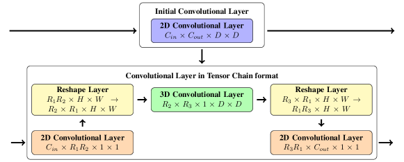
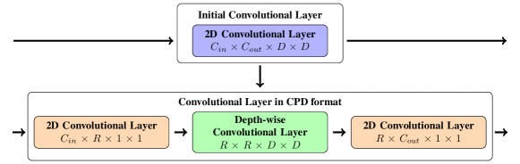
Figure 9: Graphical illustration to the proposed layer formats that show how decomposed factors are used as new weights of the compressed layer. $C_{in}$,$C_{out}$ are the number of input and output channels, $D$ is a kernel size. (a) TC layer format, $R_{1},R_{2},R_{3}$ are TC ranks, $H$ and $W$ are the input dimensions. (b) CPD layer format, $R$ is a CPD rank

H.1 TC Layer Python Implementation

class TC_layer(nn.Module): def __init__(self, layer, factors): super(TC_layer, self).__init__()

self.factors = [torch.tensor(U, dtype=torch.float32) for U in factors] self.c_in = self.factors[1].shape[1] self.c_out = self.factors[0].shape[1] self.r1 = self.factors[1].shape[0] self.r2 = self.factors[1].shape[2] self.r3 = self.factors[2].shape[2]

self.h = int(np.sqrt(self.factors[2].shape[1])) self.w = int(np.sqrt(self.factors[2].shape[1]))

self.padding = layer.padding self.stride = layer.stride self.dilation = layer.dilation self.kernel_size = layer.kernel_size self.is_bias = layer.bias is not None if self.is_bias: self.bias = layer.bias

self.conv1 = nn.Conv2d(in_channels=self.c_in, out_channels=self.r1*self.r2, kernel_size=(1, 1), bias=False) self.conv2 = nn.Conv3d(in_channels=self.r2, out_channels=self.r3, kernel_size=(1, self.h, self.w), padding=(0, self.padding[0], self.padding[1]), stride = (1, self.stride[0], self.stride[1]), bias=False) self.conv3 = nn.Conv2d(in_channels=self.r1*self.r3, out_channels=self.c_out, kernel_size=(1, 1), bias=False)

self.__replace__()

def __replace__(self): C_out, C_in, C_ker = self.factors with torch.no_grad(): self.conv1.weight = nn.Parameter(torch.tensor(C_in).permute(0, 2, 1).reshape(self.r1*self.r2, self.c_in, 1, 1)) self.conv2.weight = nn.Parameter(torch.tensor(C_ker).permute(2, 0, 1).reshape(self.r3, self.r2, 1, self.h, self.w)) self.conv3.weight = nn.Parameter(torch.tensor(C_out).permute(1, 2, 0).reshape(self.c_out, self.r1*self.r3, 1, 1)) if self.is_bias: self.conv3.bias = nn.Parameter(self.bias)

def forward(self, x): out1 = self.conv1(x) H, W = out1.shape[2], out1.shape[3] out1_reshaped = out1.view((-1, self.r1, self.r2, H, W)).permute(0, 2, 1, 3, 4) out2 = self.conv2(out1_reshaped) out2_reshaped = out2.permute(0, 2, 1, 3, 4).reshape((-1, self.r1*self.r3, int(H / self.stride[0]), int(W / self.stride[1]))) out3 = self.conv3(out2_reshaped) return out3

Appendix I Additional Experimental Results

Due to space limitations, some figures for Examples in the main manuscript are presented in Appendix. We also provide more examples and more convincing comparison between our proposed method and the existing algorithms for TC and BTD with shared coefficients. Examples in this manuscript are summarized in Table 2.

Table 2: List of Examples.

Ex.no.	Tensor size	Description	No. runs
For synthetic tensors
2	$7\times 7\times 7$, bonds $(3-3-3)$	cores with bond exceeding dimensions	10000
2	$27\times 27\times 27$, bonds $(5-5-5)$	cores with collinear factor	50
3	$9\times 9\times 9$, bond ($3-3-3$)	incomplete tensors with 50% missing elements	100
I.1		full version of Example 2
11	$10\times 10\times 10$ with bond $(4-4-4)$	extension of Example 2	100
	$15\times 15\times 15$ with bond $(6-6-6)$		100
	$20\times 20\times 20$ with bond $(8-8-8)$		100
	$25\times 25\times 25$ with bond $(10-10-10)$		100
	$30\times 30\times 30$ with bond $(12-12-12)$		100
	$35\times 35\times 35$ with bond $(14-14-14)$		100
11	$7\times 7\times 7\times 7$ with bond $(5-5-5-5)$	higher order tensors with bonds exceeding tensor dimensions	100
13	$27\times 27\times 27\times 27$ with bond ($5-5-5-5$)	higher order tensors with collinear components	50
13	$I\times I\times I\times I$ with bond $(I-I-I-I)$ where $I=10,15$	higher order tensors	200
14	$7\times 7\times 7\times 7\times 7$ with bond $13-13-\cdots-13$	order-5 tensors	100
	$3\times 3\times 3\times 3\times 3\times 3\times 3$ with bond $8-8-\cdots-8$	order-7 tensors	100
For images approximation
I.2	$128\times 128\times 3$ with bond $(R_{1}-R_{2}-R_{1})$	Six images of size $128\times 128\times 3$	2331
For compression of CNNs
6	Bonds are constrained so that the model size is close to one in CPD with rank-200	Single layer compression in ResNet-18 trained on ILSVRC-12
7	Kernels in layers 2-11 with bond $10-10-10$ Other kernels as in Example 6	Single layer compression in ResNet-18 finetuned on CIFAR-10
7	Rank selection described in Example 5	Single layer compression in ResNet-18 trained on CIFAR-10
7	As in Example 7 + CPD as in [8]	Full network compression of ResNet-18 trained on CIFAR-10
7	As in Example 7 + CPD as in [8]	Full network compression of ResNet-18 and VGG-16 trained on ILSVRC-12
I.3		extended from Example 6
I.3		extended from Examaple 7

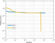
(a) Convergence of ALS and SSC

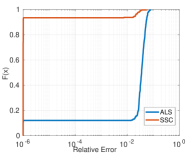
(b) Success rate of ALS and SSC

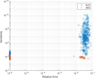
(c) Sensitivity vs Relative error

Figure 10: Performance comparison of ALS and SSC for TC decomposition in Example I.1. (a) the decomposition with SSC after 3000 ALS updates converges quickly to the exact model. (b) empirical CDF of relative errors as measure of success rate of the decomposition. SSC attains a success rate of 92% in 6000 iterations, while ALS succeeds in less than 12% with 13000 iterations. Note that the success rate of ALS in 5000 iterations is only 3%.

I.1 Examples for decomposition of synthetic tensors under difficult scenarios

Example A1 [Decomposition of tensor of size $7\times 7\times 7$ with bond $(3-3-3)$.]

This is an extension of Example 2 in the main manuscript. For the same tensors as in Example 2, we applied sensitivity correction after 3000 ALS updates, then continued the decomposition, the ALS+SSC converged quickly to the exact solution.Figure 10(a) compares convergences between ALS and SSC in one decomposition of the tensor. Similar convergence behavior can be observed in many other decompositions. SSC improves the convergence of the TC decomposition and gives a success rate of 92% as shown in Figure 10(b). A decomposition is a success if it achieves a relative approximation error smaller than $10^{-6}$

$$\frac{\|\boldsymbol{\mathscr{{Y}}}-\hat{\boldsymbol{\mathscr{{Y}}}}\|_{F}^{2}}{\|\boldsymbol{\mathscr{{Y}}}\|_{F}^{2}}\leq 10^{-6}\,.$$ (28)

We use the empirical cdf of the relative approximation error as a measure of the success rate. There are 10000 decompositions for 100 tensors; each tensor is decomposed 100 times with different initial points.

Figure 10(c) shows scatter plots of the sensitivity measures and relative approximation errors of estimated tensors. The results obtained by ALS often have very high sensitivity, making the algorithm hard to explain the data fully.

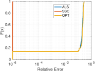
(a) Tensor dimensions $I=10$ with bond $R=4$

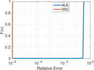
(b) Tensor dimensions $I=15$ with bond $R=6$

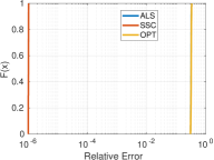
(c) Tensor dimensions $I=20$ with bond $R=8$

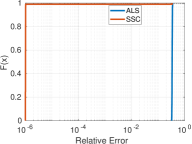
(d) Tensor dimensions $I=25$ with bond $R=10$

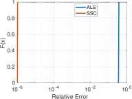
(e) Tensor dimensions $I=30$ with bond $R=12$

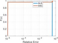
(f) Tensor dimensions $I=35$ with bond $R=14$

Figure 11: Success rates for TC decomposition of tensors of size $I\times I\times I$ with bond dimensions $(R-R-R)$ in Example 11. ALS and OPT failed in our example. We can decompose the tensors with very high success rates using the proposed algorithm for sensitivity correction and sensitivity control.

Example A2 [More TC decomposition for tensors of order-3]

Similar to Example I.1, we decomposed order-3 tensors of dimensions $I\times I\times I$ and bond dimensions $(R-R-R)$. We applied ALS and OPT algorithms in the examples and ran the two algorithms within 6000 iterations. SSC was used to correct the sensitivity of the estimated tensors after 1000 ALS updates. Figure 11 reports success rates of the considered algorithms. For tensors of size $10\times 10\times 10$ with bond dimensions $(4-4-4)$, ALS and OPT have low success rates, less than 14% over 100 decompositions. For bigger tensors with larger bond dimensions, the two algorithms completely fail. Since OPTs are more expensive than ALS and its performances are not much different from ALS, we provide simulation results for OPT for tensors with small sizes.

The proposed algorithm, SSC, has significantly improved the performances of the ALS algorithm. In all the tests, we obtained nearly perfect decomposition with relative approximation error less than $10^{-6}$.

Example A3 [TC decompositions for order-4 tensors]

Similar to Example I.1, we show TC decomposition for order-4 tensors of size $7\times 7\times 7\times 7$ with bond dimensions (5-5-5-5), i.e., the corresponding factor matrices have more columns than rows. Figure 12(a) shows ALS and OPT[22, 57] got stuck in false local minima after several hundreds of iterations, whereas intensity (red curve) and sensitivity (blue curve) of the estimated tensors grow to $10^{8}$ shown in Figure 12(b). This example confirms the instability problem for TC of higher order.

We applied the Sensitivity correction method, and suppressed the sensitivity of the estimated tensor from $10^{7}$ to several hundred, then continued the decomposition from a new tensor with much smaller sensitivity. The correction method helped us achieving a perfect decomposition (see Figure 12(a)).

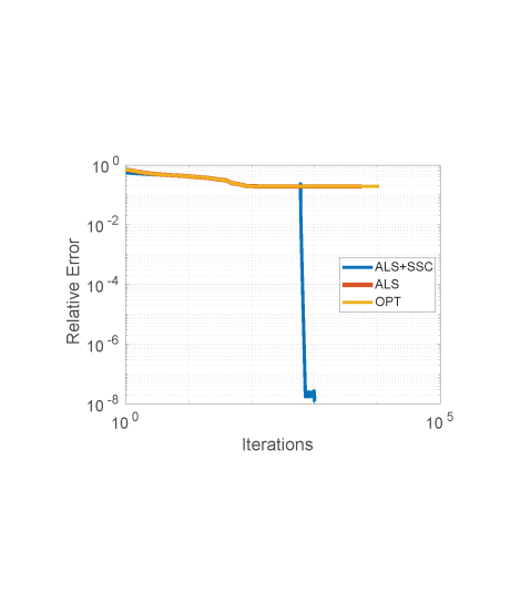
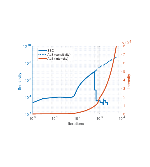
Figure 12: Illustration for performances obtained by algorithms used in Example 11. Tensors are of size $7\times 7\times 7\times 7$ with bond $(5-5-5-5)$. After SS correction, we obtain a new estimated tensor with low sensitivity (see blue curve in (b)). TC decomposition (ALS+SS) quickly converged after the sensitivity correction (blue curve in (a)).

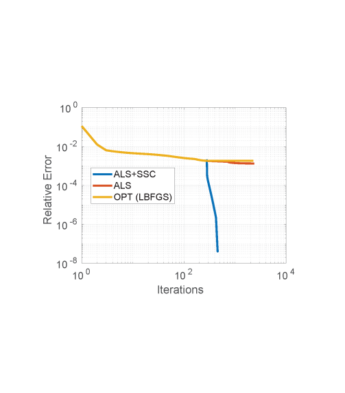
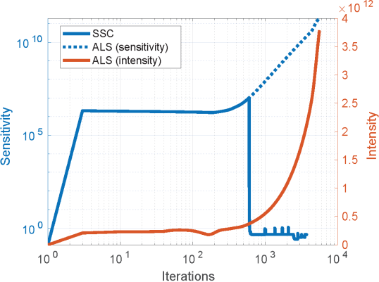
Figure 13: Performances obtained by algorithms for decomposition of tensors of size $27\times 27\times 27\times 27$ in Example 13. ALS+SS is the ALS plus sensitivity correction. Intensity of the estimated tensors using ALS exceeds $3.5\,10^{12}$, and the sensitivity of the tensor is greater than $2\,10^{10}$, while the algorithm converges slowly after 1000 iterations.

Example A4 [TC decompositions for order-4 tensors with highly collinear components]

We demonstrate TC of higher order tensors, $\boldsymbol{\mathscr{{Y}}}=\mathopen{{\stackengine{.25ex}{[}{{\scaleto{\circlearrowright}{1.1ex}}}{O}{c}{F}{F}{L}}}\boldsymbol{\mathscr{{U}}}1,\boldsymbol{\mathscr{{U}}}_{2},\boldsymbol{\mathscr{{U}}}_{3},\boldsymbol{\mathscr{{U}}}_{4}\mathclose{{\stackengine{.25ex}{]}{\hskip 0.86108pt{\scaleto{\circlearrowleft}{1.1ex}}}{O}{c}{F}{F}{L}}}$ which are similar to those in Example 2 in the main text, but of order-4 with size $27\times 27\times 27\times 27$ and bond dimensions (ranks) $(5-5-5-5)$. The factor matrices ${{\bf U}}_{n}$ comprise three blocks, ${{\bf U}}_{n}(:,1:9)$, ${{\bf U}}_{n}(:,10:18)$ and ${{\bf U}}_{n}(:,19:25)$, columns in each block are highly collinear. Figure 13 shows that the relative approximation errors using ALS are far from zero. Similar to the previous examples, with sensitivity correction, we can correct the estimated tensors with high sensitivity to a new estimation with sensitivity less than 10 (Figure 13). The decomposition converged quickly after the correction as seen in Figure 13.

Example A5 [More TC decompositions for order-4 tensors]

In this example, we decompose order-4 tensors of size $I\times I\times I\times I$ with bond dimensions $(I-I-I-I)$, where $I=10,15$. The success rates of the three considered algorithms, ALS, OPT, and ALS plus sensitivity correction and control (SSC), are compared in Figure 14. Both ALS and OPT failed to decompose a tensor of order-4 with large core tensors. However, with SSC, ALS attained a success rate of 99-100%.

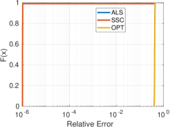
(a) Tensor dimension $I=10$

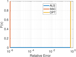
(b) Tensor dimension $I=15$

Figure 14: Success rate of TC algorithms in decomposition of tensors of size $I\times I\times I\times I$ with bond $(I-I-I-I)$ in Example 13. Both ALS and OPT fail in decomposition of tensor of order-4 with big core tensors.

Example A6 [More TC decompositions for higher order tensors]

In this example, we decompose order-5 tensors of size $I\times I\cdots\times I$ with bond dimensions $(R-R-\cdots-R)$, where $I=7$ and $R=13$, and order-7 tensors with dimensions $I=3$ and bond $R=8$. Convergence of algorithms versus iterations is shown Figure 15 and Figure 16(c). Like other TC decomposition for tensors of order-3,4, besides ALS and OPT, we tried several other TC algorithms, but none succeeded.

The success rates of the three considered algorithms, ALS, OPT, and ALS plus sensitivity correction and control (SSC), are compared in Figure 15(c) and Figure 16(c). Both ALS and OPT failed to decompose tensor of order-4 with large core tensors. However, with SSC, ALS attained a success rate of 99-100%.

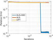
(a) Convergence of ALS, OPT and ALS+SSC

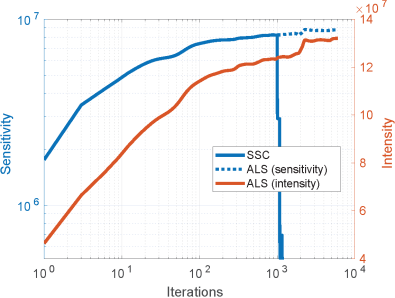
(b) Sensitivity of ALS

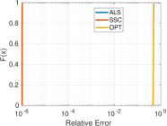
(c) Success rate

Figure 15: Illustration for performances for decomposition of tensors of order-5 and size $7\times 7\times 7\times 7\times 7$ in Example 14.

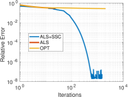
(a) Convergence of ALS, OPT and ALS+SSC

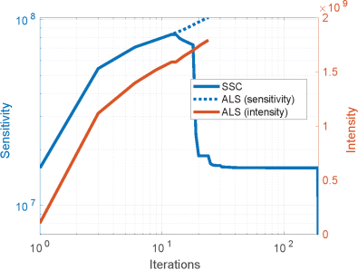
(b) Sensitivity

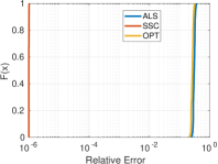
(c) Success Rate

Figure 16: Illustration for performances for decomposition of tensors of order-7 and size $3\times 3\times\cdots\times 3$ with bond dimensions $R=8$ in Example 14

.

I.2 Fitting Images by TC-decomposition

Example A7 [TC for image approximation]

Figure 17: Images used in Example I.2.

We fit six images of size $128\times 128\times 3$ shown in in Figure 17, by TC models with various bond dimensions $(R_{1},R_{2},R_{3}=R_{1})$. $R_{1}=2,\ldots,40$ and $R_{2}\geq 2$ such that the number of parameters of TC models should not exceed the number of data elements, i.e., $49152$. There are in total 388-392 TC decompositions for each image.

$$\#TC(R_{1},R_{2},R_{1})=256R_{1}R_{2}+3R_{1}^{2}\leq 49152$$ (29)

For the same approximation bound, we compare three models obtained using ALS, ALS with sensitivity correction, and algorithm with Sensitivity Control

$$\|\boldsymbol{\mathscr{{Y}}}-\boldsymbol{\mathscr{{X}}}\|_{F}\leq\epsilon\,\|\boldsymbol{\mathscr{{Y}}}\|_{F}$$

Figure 18 compares the approximation errors for different bond dimensions.

For the ”Peppers” image, the SSC significantly improves the approximation error for the same TC model. In other words, SSC allows us to choose a smaller TC model with the same approximation error bound than using ALS (or any other algorithms for TC). For example, at the approximation error bound of $0.02$, SSC gives the TC model with bond $(6-16-6)$, which comprises 24684 parameters, and attains a relative approximation error of $0.01927<0.02$. For the same bond dimensions, ALS converges to a model with an approximation error of $0.0331>0.02$. In order to attain the same accuracy, ALS procedures a TC model with bond dimensions of $(6-21-6)$ or $(7-18-7)$, which have 32364 or 32403 parameters, i.e., demanding 7719 more parameters than the model estimated by SSC.

The improvements are even significant for TC decomposition with high accuracy, i.e., low approximation error. Not only for the ‘’Pepper” image, but Figure 18 also shows that SSC gains performance of ALS for approximation of the other images.

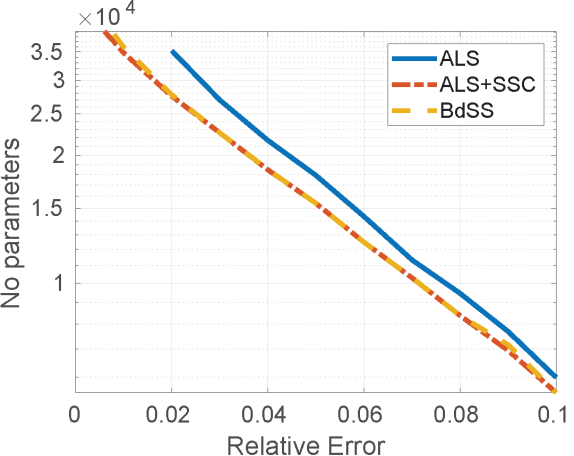
(a) Mandrill

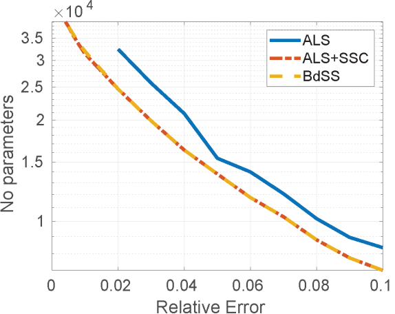
(b) Peppers

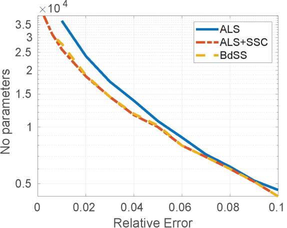
(c) Lena

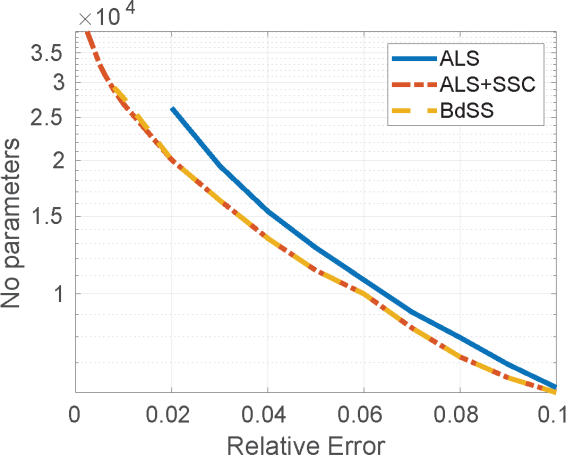
(d) Barbara

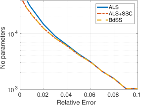
(e) Tiffany

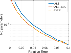
(f) House

Figure 18: Comparison of TC models which approximate images in Example I.2.

I.3 CNN compression

Example A8 [extended from Example 6] Figure 19 compares convergence of the decomposition of convolutional kernels using ALS and SSC. A similar comparison is presented in Figure 5. SSC was applied after 3000 ALS updates, and the decomposition resumed with 3000 ALS updates. Decompositions using only ALS could not achieve the approximation errors obtained by SSC.

Example A9 [extended from Example 7] SSC achieves smaller approximation errors, and yields estimated models with smaller sensitivity. This helps the new neural networks to fine-tune easier. In Figure 20, we provide more comparisons between the learning curves of two versions of ResNet-18 after replacing one convolutional layer by a TC-layer, one with convolutional kernels estimated using SSC, and another one obtained by ALS. Similar curves are presented in Figure 7(c). In most examples, neural networks without SSC cannot attain the original accuracy of ResNet-18, e.g., convolutional layers 4, 5, 6, 9, 10, 12, 14, 15, 16, 17, or need much more number iterations than the networks using TC-SSC, e.g., layer 3. Except for the network with TC-layer applied to the convolutional layer 11, we observe a slight difference between the two learning curves.

In addition to single compression, we perform full model compression of ResNet-18. TC-layers replace all convolutional layers. Figure 21 shows that the new ResNet-18 with kernels estimated using ALS could not attain the original accuracy of 92.29% for CIFAR-10. A similar ResNet-18 but weights in all TC-layers estimated with SSC can recover the initial accuracy after fine-tuning.

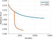
(a) Convolutional layer 3

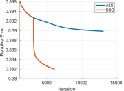
(b) Convolutional layer 4

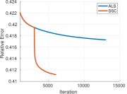
(c) Convolutional layer 5

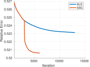
(d) Convolutional layer 6

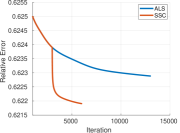
(e) Convolutional layer 7

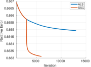
(f) Convolutional layer 9

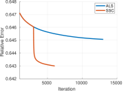
(g) Convolutional layer 10

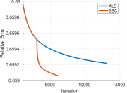
(h) Convolutional layer 11

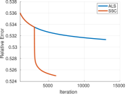
(i) Convolutional layer 12

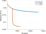
(j) Convolutional layer 14

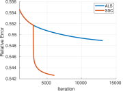
(k) Convolutional layer 15

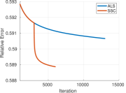
(l) Convolutional layer 16

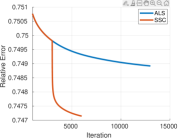
(m) Convolutional layer 17

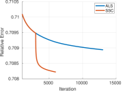
(n) Convolutional layer 19

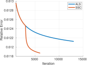
(o) Convolutional layer 20

Figure 19: Relative approximation errors as function of iterations illustrate convergence of the decomposition of convoluional kernels using ALS and SSC.

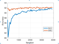
(a) Convolutional layer 3

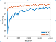
(b) Convolutional layer 4

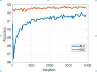
(c) Convolutional layer 5

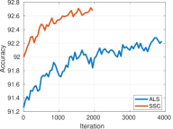
(d) Convolutional layer 6

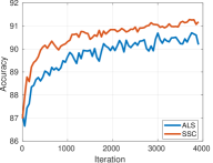
(e) Convolutional layer 9

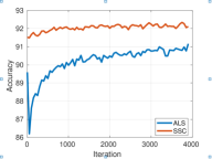
(f) Convolutional layer 10

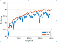
(g) Convolutional layer 11

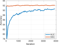
(h) Convolutional layer 12

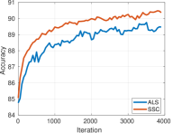
(i) Convolutional layer 14

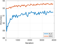
(j) Convolutional layer 15

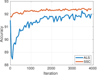
(k) Convolutional layer 16

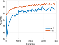
(l) Convolutional layer 17

Figure 20: Learning curves for single layer compression of ResNet-18 finetuned on CIFAR-10 for Example 7. Neural networks with TC layers whose convolutional coefficients are obtained by SSC are easier to train and converge faster than the same neural networks with weights estimated using ALS.

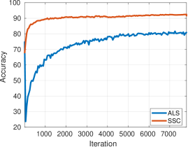
Figure 21: Accuracy of two new ResNet-18 with all convolutional kernels replaced by TC layers in Example 7. The network whose kernels are estimated using ALS could not attain the original accuracy of ResNet-18 for CIFAR-10, 92.29%. The network can reach the initial accuracy if the weights in all TC-layers are estimated using SSC.

References

- [1] Joseph M. Landsberg. Tensors: Geometry and Applications, volume 128. American Mathematical Society, Providence, RI, USA, 2012.
- [2] S. Handschuh. Numerical Methods in Tensor Networks. PhD thesis, Facualty of Mathematics and Informatics, University Leipzig, Germany, Leipzig, Germany, 2015.
- [3] Yi Guo, Huan Yuan, Jianchao Tan, Zhangyang Wang, Sen Yang, and Ji Liu. Gdp: Stabilized neural network pruning via gates with differentiable polarization. In Proceedings of the IEEE/CVF International Conference on Computer Vision (ICCV), pages 5239–5250, October 2021.
- [4] Sidak Pal Singh and Dan Alistarh. Woodfisher: Efficient second-order approximation for neural network compression. In H. Larochelle, M. Ranzato, R. Hadsell, M. F. Balcan, and H. Lin, editors, Advances in Neural Information Processing Systems, volume 33, pages 18098–18109. Curran Associates, Inc., 2020.
- [5] Vladimir Kryzhanovskiy, Gleb Balitskiy, Nikolay Kozyrskiy, and Aleksandr Zuruev. Qpp: Real-time quantization parameter prediction for deep neural networks. In Proceedings of the IEEE/CVF Conference on Computer Vision and Pattern Recognition (CVPR), pages 10684–10692, June 2021.
- [6] Miao Yin, Siyu Liao, Xiao-Yang Liu, Xiaodong Wang, and Bo Yuan. Towards extremely compact rnns for video recognition with fully decomposed hierarchical tucker structure. In Proceedings of the IEEE/CVF Conference on Computer Vision and Pattern Recognition (CVPR), pages 12085–12094, June 2021.
- [7] Hyeji Kim, Muhammad Umar Karim Khan, and Chong-Min Kyung. Efficient neural network compression. In Proceedings of the IEEE/CVF Conference on Computer Vision and Pattern Recognition (CVPR), pages 12569–12577, June 2019.
- [8] A.-H. Phan, K. Sobolev, K. Sozykin, D. Ermilov, J. Gusak, P. Tichavský, V. Glukhov, I. Oseledets, and A. Cichocki. Stable low-rank tensor decomposition for compression of convolutional neural network. In Computer Vision – ECCV 2020, 2020.
- [9] Yannis Panagakis, Jean Kossaifi, Grigorios G. Chrysos, James Oldfield, Mihalis A. Nicolaou, Anima Anandkumar, and Stefanos Zafeiriou. Tensor methods in computer vision and deep learning. Proceedings of the IEEE, 109(5):863–890, 2021.
- [10] Alexander Novikov, Dmitry Podoprikhin, Anton Osokin, and Dmitry Vetrov. Tensorizing neural networks. In Proceedings of the 28th International Conference on Neural Information Processing Systems - Volume 1, NIPS’15, pages 442–450, Cambridge, MA, USA, 2015. MIT Press.
- [11] Miao Yin, Yang Sui, Siyu Liao, and Bo Yuan. Towards efficient tensor decomposition-based dnn model compression with optimization framework. In Proceedings of the IEEE/CVF Conference on Computer Vision and Pattern Recognition (CVPR), pages 10674–10683, June 2021.
- [12] Emily L Denton, Wojciech Zaremba, Joan Bruna, Yann LeCun, and Rob Fergus. Exploiting linear structure within convolutional networks for efficient evaluation. In Z. Ghahramani, M. Welling, C. Cortes, N. Lawrence, and K. Q. Weinberger, editors, Advances in Neural Information Processing Systems, volume 27, pages 1269–1277. Curran Associates, Inc., 2014.
- [13] L. R. Tucker. Implications of factor analysis of three-way matrices for measurement of change. Problems in measuring change, 15:122–137, 1963.
- [14] Yong-Deok Kim, Eunhyeok Park, Sungjoo Yoo, Taelim Choi, Lu Yang, and Dongjun Shin. Compression of deep convolutional neural networks for fast and low power mobile applications. In 4th International Conference on Learning Representations, ICLR 2016, 2016.
- [15] L. De Lathauwer. Decompositions of a higher-order tensor in block terms – Part I and II. SIAM Journal on Matrix Analysis and Applications (SIMAX), 30(3):1022–1066, 2008. Special Issue on Tensor Decompositions and Applications.
- [16] B.N. Khoromskij. -quantics approximation of - tensors in high-dimensional numerical modeling. Constructive Approximation, 34(2):257–280, 2011.
- [17] M. Espig, W. Hackbusch, S. Handschuh, and R. Schneider. Optimization problems in contracted tensor networks. Comput. Visual. Sci., 14(6):271–285, 2011.
- [18] Joseph M. Landsburg, Yang Qi, and Ke Ye. On the geometry of tensor network states. Quantum Inf. Comput., 12(3-4):346–354, 2012.
- [19] I.V. Oseledets and E.E. Tyrtyshnikov. TT-cross approximation for multidimensional arrays. Linear Algebra and its Applications, 432(1):70–88, 2010.
- [20] Laurent Sorber, Marc Van Barel, and Lieven De Lathauwer. Structured data fusion. IEEE Journal of Selected Topics in Signal Processing, 9(4):586–600, 2015.
- [21] Petr Tichavský, Anh-Huy Phan, and Andrzej Cichocki. Krylov-levenberg-marquardt algorithm for structured tucker tensor decompositions. IEEE Journal of Selected Topics in Signal Processing, 15(3):550–559, 2021.
- [22] Longhao Yuan, Jianting Cao, Xuyang Zhao, Qiang Wu, and Qibin Zhao. Higher-dimension tensor completion via low-rank tensor ring decomposition. In Asia-Pacific Signal and Information Processing Association Annual Summit and Conference, APSIPA ASC 2018, Honolulu, HI, USA, November 12-15, 2018, pages 1071–1076. IEEE, 2018.
- [23] M. Espig, K. K. Naraparaju, and J. Schneider. A note on tensor chain approximation. Computing and Visualization in Science, 15(6):331–344, Dec 2012.
- [24] Qibin Zhao, Guoxu Zhou, Shengli Xie, Liqing Zhang, and Andrzej Cichocki. Tensor Ring Decomposition. arXiv preprint arXiv:1606.05535, 2016.
- [25] W. Wang, V. Aggarwal, and S. Aeron. Efficient Low Rank Tensor Ring Completion. In 2017 IEEE International Conference on Computer Vision (ICCV), pages 5698–5706, Oct 2017.
- [26] M Salman Asif and Ashley Prater-Bennette. Low-Rank Tensor Ring Model for Completing Missing Visual Data. In ICASSP 2020-2020 IEEE International Conference on Acoustics, Speech and Signal Processing (ICASSP), pages 5415–5419. IEEE, 2020.
- [27] Oscar Mickelin and Sertac Karaman. On Algorithms for and Computing with the Tensor Ring Decomposition. Numerical Linear Algebra with Applications, 2020.
- [28] Wei He, Naoto Yokoya, Longhao Yuan, and Qibin Zhao. Remote Sensing Image Reconstruction Using Tensor Ring Completion and Total Variation. IEEE Transactions on Geoscience and Remote Sensing, 57(11):8998–9009, 2019.
- [29] Huyan Huang, Yipeng Liu, Zhen Long, and Ce Zhu. Robust low-rank tensor ring completion. IEEE Transactions on Computational Imaging, 6:1117–1126, 2020.
- [30] Abdul Ahad, Zhen Long, Ce Zhu, and Yipeng Liu. Hierarchical Tensor Ring Completion. arXiv preprint arXiv:2004.11720, 2020.
- [31] Jinshi Yu, Guoxu Zhou, Chao Li, Qibin Zhao, and Shengli Xie. Low tensor-ring rank completion by parallel matrix factorization. IEEE Transactions on Neural Networks and Learning Systems, 32(7):3020–3033, 2021.
- [32] Meng Ding, Ting-Zhu Huang, Xi-Le Zhao, and Tian-Hui Ma. Tensor completion via nonconvex tensor ring rank minimization with guaranteed convergence. Signal Processing, 194:108425, 2022.
- [33] Yang Xu, Zebin Wu, Jocelyn Chanussot, and Zhihui Wei. Hyperspectral images super-resolution via learning high-order coupled tensor ring representation. IEEE Transactions on Neural Networks and Learning Systems, 31(11):4747–4760, 2020.
- [34] Zhiyu Cheng, Baopu Li, Yanwen Fan, and Yingze Bao. A Novel Rank Selection Scheme in Tensor Ring Decomposition Based on Reinforcement Learning for Deep Neural Networks. In ICASSP 2020-2020 IEEE International Conference on Acoustics, Speech and Signal Processing (ICASSP), pages 3292–3296. IEEE, 2020.
- [35] Farnaz Sedighin, Andrzej Cichocki, and Anh-Huy Phan. Adaptive rank selection for tensor ring decomposition. IEEE Journal of Selected Topics in Signal Processing, 15(3):454–463, 2021.
- [36] L. Sorber, M. Van Barel, and L. De Lathauwer. Tensorlab v1.0, February 2013.
- [37] Jin-Young Choi and Chong-Ho Choi. Sensitivity analysis of multilayer perceptron with differentiable activation functions. IEEE Trans. Neural Networks, 3(1):101–107, 1992.
- [38] Daniel S. Yeung, Ian Cloete, Daming Shi, and Wing W. Y. Ng. Sensitivity Analysis for Neural Networks. Natural Computing Series. Springer, 2010.
- [39] Lin Xiang, Xiaoqin Zeng, Shengli Wu, Yanjun Liu, and Baohua Yuan. Computation of cnn’s sensitivity to input perturbation. Neural Process. Lett., 53(1):535–560, 2021.
- [40] Roman Novak, Yasaman Bahri, Daniel A. Abolafia, Jeffrey Pennington, and Jascha Sohl-Dickstein. Sensitivity and generalization in neural networks: an empirical study. CoRR, abs/1802.08760, 2018.
- [41] Jaime Pizarroso, José Portela, and Antonio Muñoz. Neuralsens: Sensitivity analysis of neural networks. CoRR, abs/2002.11423, 2020.
- [42] Z. Wen and W. Yin. A feasible method for optimization with orthogonality constraints. Mathematical Programming, pages 1–38, 2012.
- [43] Walter Gander, Gene H. Golub, and Urs von Matt. A constrained eigenvalue problem. Linear Algebra and its Applications, 114-115:815–839, 1989. Special Issue Dedicated to Alan J. Hoffman.
- [44] A.-H. Phan, P. Tichavský, and A. Cichocki. Error preserving correction: A method for CP decomposition at a target error bound. IEEE Transactions on Signal Processing, 67(5):1175–1190, March 2019.
- [45] A.-H. Phan, M. Yamagishi, and A. Cichocki. Quadratic programming over ellipsoids and its applications to linear regression and tensor decomposition. Neural Computing and Applications, 32:7097–7120, 2020.
- [46] V. Aggarwal, W. Wang, B. Eriksson, Y. Sun, and W. Wang. Wide compression: Tensor ring nets. In 2018 IEEE/CVF Conference on Computer Vision and Pattern Recognition (CVPR), pages 9329–9338, Los Alamitos, CA, USA, jun 2018. IEEE Computer Society.
- [47] Karen Simonyan and Andrew Zisserman. Very deep convolutional networks for large-scale image recognition. In 3rd International Conference on Learning Representations, ICLR, 2015.
- [48] K. He, X. Zhang, S. Ren, and J. Sun. Deep residual learning for image recognition. In 2016 IEEE Conference on Computer Vision and Pattern Recognition (CVPR), pages 770–778, 2016.
- [49] Jia Deng, Wei Dong, Richard Socher, Li-Jia Li, Kai Li, and Li Fei-Fei. Imagenet: A large-scale hierarchical image database. 2009 IEEE Conference on Computer Vision and Pattern Recognition (CVPR), pages 248–255, 2009.
- [50] Alex Krizhevsky. Learning multiple layers of features from tiny images. Technical Report TR-2009, University of Toronto, Toronto, 2009.
- [51] X. Zhang, J. Zou, K. He, and J. Sun. Accelerating very deep convolutional networks for classification and detection. IEEE Transactions on Pattern Analysis and Machine Intelligence, 38(10):1943–1955, 2016.
- [52] Zhuangwei Zhuang, Mingkui Tan, Bohan Zhuang, Jing Liu, Yong Guo, Qingyao Wu, Junzhou Huang, and Jinhui Zhu. Discrimination-aware channel pruning for deep neural networks. In Advances in Neural Information Processing Systems, pages 883–894, 2018.
- [53] Xitong Gao, Yiren Zhao, Łukasz Dudziak, Robert Mullins, and Cheng-Zhong Xu. Dynamic channel pruning: Feature boosting and suppression. In International Conference on Learning Representations, 2019.
- [54] Julia Gusak, Maksym Kholyavchenko, Evgeny Ponomarev, Larisa Markeeva, Philip Blagoveschensky, Andrzej Cichocki, and Ivan Oseledets. Automated multi-stage compression of neural networks. 2019 IEEE/CVF International Conference on Computer Vision Workshop (ICCVW), pages 2501–2508, 2019.
- [55] Weizhe Hua, Yuan Zhou, Christopher M De Sa, Zhiru Zhang, and G. Edward Suh. Channel gating neural networks. In H. Wallach, H. Larochelle, A. Beygelzimer, F. d’Alché Buc, E. Fox, and R. Garnett, editors, Advances in Neural Information Processing Systems 32, pages 1886–1896. 2019.
- [56] Yu Pan, Jing Xu, Maolin Wang, Jinmian Ye, Fei Wang, Kun Bai, and Zenglin Xu. Compressing Recurrent Neural Networks with Tensor Ring for Action Recognition. In Proceedings of the AAAI Conference on Artificial Intelligence, volume 33, pages 4683–4690, 2019.
- [57] Daniel M. Dunlavy, Tamara G. Kolda, and Evrim Acar. Poblano v1.0: A matlab toolbox for gradient-based optimization. Technical Report SAND2010-1422, Sandia National Laboratories, March 2010.