An SDP Relaxation for the Sparse Integer Least Square Problem

An SDP Relaxation for the Sparse Integer Least Square Problem

Abstract

In this paper, we study the polynomial approximability or solvability of sparse integer least square problem (SILS), which is the NP-hard variant of the least square problem, where we only consider sparse $\{0,\pm 1\}$-vectors. We propose an $\ell_{1}$-based SDP relaxation to SILS, and introduce a randomized algorithm for SILS based on the SDP relaxation. In fact, the proposed randomized algorithm works for a broader class of binary quadratic program with cardinality constraint, where the objective function can be possibly non-convex. Moreover, when the sparsity parameter is fixed, we provide sufficient conditions for our SDP relaxation to solve SILS. The class of data input which guarantee that SDP solves SILS is broad enough to cover many cases in real-world applications, such as privacy preserving identification, and multiuser detection. To show this, we specialize our sufficient conditions to two special cases of SILS with relevant applications: the feature extraction problem and the integer sparse recovery problem. We show that our SDP relaxation can solve the feature extraction problem with sub-Gaussian data, under some weak conditions on the second moment of the covariance matrix. We also show that our SDP relaxation can solve the integer sparse recovery problem under some conditions that can be satisfied both in high and low coherence settings.

Key words: Semidefinite relaxation, Sparsity, Integer least square problem, $\ell_{1}$ relaxation

1 Introduction

The Integer Least Square problem is a fundamental NP-hard optimization problem which arises from many real-world applications, including communication theory, lattice design, Monte Carlo second-moment estimation, and cryptography. We refer readers to the comprehensive survey [1] and references therein. In the integer least square problem, we are given an $n\times d$ matrix $M$, a $d$-vector $b$, and we seek the closest point to $b$, in the lattice spanned by the columns of $M$. The ILS problem can be formulated as the following optimization problem:

$$\min \frac{1}{n}\left\lVert Mx-b\right\rVert_{2}^{2}$$ (ILS)

s.t. $$x\in\mathbb{Z}^{d}.$$

In many scenarios, one is only interested in sparse solutions to (ILS), i.e., vectors $x$ with a large fraction of entries equal to zero. This is primarily motivated by the need to recover a sparse signal [31, 53], or the need to improve the efficiency of data structure representation [39]. Applications include cyber security [31], array signal processing [53], and sparse code multiple access [13]. In this sparse setting, the feasible region is often further restricted to the set $\{0,\pm 1\}^{d}$. Applications can be found in multiuser detection, where user terminals transmit binary symbols in a code-division multiple access (CDMA) system [57], in sensor networks, where sensors with low duty cycles are either silent (transmit $0$) or active (transmit $\pm 1$) [44], and in privacy preserving identification, where a sparse vector in $\{0,\pm 1\}$ is employed to approximate the ‘content’ of feature data [39]. In this paper, we study this version of (ILS), where we only consider sparse solutions with entries in $\{0,\pm 1\}$. Formally, in the sparse integer least square problem, an instance consists of an $n\times d$ matrix $M$, a vector $b\in\mathbb{R}^{n}$, and a positive integer $\sigma\leq d$. Our task is to find a vector $x$ which solves the optimization problem (1) or its variant (1), defined as follows:

—s—[0]¡break¿ 1n∥M x -b∥_2^2 x∈{0, ±1}^d ∥x∥_0 ≤σ, —s—[0]¡break¿ 1n∥M x -b∥_2^2 x∈{0, ±1}^d ∥x∥_0 = σ.

One can interpret (1) as (1) with extra information or belief on the optimal choice of sparsity of the optimal solution.

As we will see in Theorem 1 in Section 2, Problem (1) and (1) are NP-hard in their full generality. In this paper, we are interested in polynomial running time algorithms that either obtain an approximated optimal solution to Problem (1), or obtain an exact optimal solution to Problem (1) provided some assumptions on the data input are satisfied. To be best of our knowledge, the only known result is in [5]. The authors propose a sparse sphere decoding algorithm which returns an optimal solution to Problem (1). They also show that this algorithm has an expected running time which is polynomial in $d$, in the case where $M$ has i.i.d. standard Gaussian entries and there exists a sparse integer vector $z^{*}\in\{0,\pm 1\}^{d}$ such that the residual vector $b-Mz^{*}$ is comprised of i.i.d. Gaussian entries. However, this algorithm results in an exponential running time at the presence of a nonsparse $z^{*}$. Algorithms for Problem (1) with a non-polynomial running time include sparsity-exploiting sphere decoding-based MUD [57] and integer quadratic optimization algorithms (see, e.g., [7] and references therein). Efficient algorithms for Problem (1) with no theoretical guarantee on the quality of the solution can be found in [57, 44], where the authors proposed sparsity-exploiting decision-directed MUD, Lasso-based convex relaxation methods, and CoSaMP. Problem (1) has aroused many interests as well. Practical algorithms for Problem (1) include SF-OMP [45], and discrete valued sparse ADMM algorithm [43]. However, these two algorithm also do not have guarantees on the quality of their solutions.

Our contribution. In this paper, we further the understanding of the limits of computations for Problem (1) and Problem (1). We provide a randomized algorithm that finds a feasible solution to (1) with high probability, and shows an approximation gap. Then, we obtain a broad class of data input which guarantee that (1) can be solved efficiently. To be concrete, in Section 3 we give an $\ell_{1}$-based semidefinite relaxation to (1) and (1), denoted by (3) and (3), respectively. These two relaxations only differ at one single linear matrix inequality constraint. It is known that semidefinite programming (SDP) problems can be solved in polynomial time up to an arbitrary accuracy, by means of the ellipsoid algorithm and interior point methods [47, 29]. Recent studies have witnessed great success of SDP relaxations in (i) solving structured integer quadratic optimization problems in polynomial time, and (ii) finding the hidden sparse structure of a given mathematical object. Examples include clustering [26], sparse principal component analysis [2], sparse support vector machine [11], sub-Gaussian mixture model [18], community detection problem [25], and so on. Note that problems (1) and (1) are also by nature integer quadratic optimization problems with a sparsity constraint, so it is natural and well-motivated to seek for an effective SDP relaxations. In Section 4, we proposed a randomized algorithm, Algorithm 1, for (1). In fact, our randomized algorithm will not only work for (1), but for any binary quadratic programs with cardinality constraint (4), provided that the coefficient matrix of the quadratic function has non-negative diagonal entries. Thus, Algorithm 1 can handle some non-convex quadratic objectives as well. The input of Algorithm 1 consists of an (approximated) optimal solution to (3), and two threshold constant $T$ and $C$; the output is a $d$-vector $\bar{x}$ in $\{0,\pm 1\}$. We show in Theorem 2 that $\bar{x}$ is feasible to (1) with high probability, and the expected objective function is a $1/T^{2}$ multiple of the optimal value, after substracting an additional term that depends on $T,C$ and the input data $(M,b,\sigma)$. It can be shown that when $\sigma\ll T$, the additional term will diminish as $(\sigma,T)\rightarrow\infty$, and hence Algorithm 1 is an asymptotic $1/T^{2}$-approximation algorithm. To the best of our knowledge, Algorithm 1 is the first known randomized algorithm for (1) that has a theoretical guarantee. Then, we focus on (1). One can conceive (1) to be (1) where the optimal sparsity parameter is known. We found that in this case, our proposed SDP relaxation shows stronger power than one will expect. In particular, we show that (3) is able to solve (1) under several diverse sets of input $(M,b,\sigma)$, suggesting that it is a very flexible relaxation. We give both theoretical and computational evidence, aiming to explain the flexibility of (3). In Theorems 3 and 4 in Section 5, we provide sufficient conditions for (3) to find a unique optimal solution to (1). To the best of our knowledge, our results are the first ones that study the polynomial solvability of (1) in its full generality. Furthermore, we illustrate that our proposed sufficient conditions can be easily verified in some practical situation, based on a quantity known as matrix coherence. To be formal, we define the coherence of a positive semidefinite matrix $\Psi$ to be

$$\mu(\Psi) :=\max_{i\neq j}\frac{|\Psi_{ij}|}{\sqrt{|\Psi_{ii}\Psi_{jj}|}},$$ (1)

where we assume $0/0=0$ if necessary. Recently, matrix coherence has aroused much attention in compressed sensing [17] and in sparsity-aware learning [46], thanks to its ease of computation and connection to the ability to recover a sparse optimal solution [37]. In this paper, we say that a model has a high coherence if we have $\mu(M^{\top}M)=\omega(1/\sigma)$, while it has a low coherence if we have $\mu(M^{\top}M)=\mathcal{O}(1/\sigma)$. In particular, in Corollary 5, we give sufficient conditions for (3) to solve (1), which are tailored to low coherence models.

Next, in Sections 6 and 7, we showcase the power and flexibility of (3), by showing that it is able to nicely solve two problems of interest related to (1): the feature extraction problem and the integer sparse recovery problem. All these results will be consequences of Theorems 3 and 4. The input to both the feature extraction problem and the integer sparse recovery problem is the same as the input to (1): we are given an $n\times d$ matrix $M$, a vector $b\in\mathbb{R}^{n}$, and a positive integer $\sigma\leq d$. One key difference with general (1) is that the data input in these two problems satisfies

$$b=Mz^{*}+\epsilon,$$ (LM)

for some ground truth vector $z^{*}\in\mathbb{R}^{d}$ and for some small noise vector $\epsilon\in\mathbb{R}^{n}$. Note that, in this setting, $z^{*}$ and $\epsilon$ are unknown, i.e., they are not part of the input of the problem. The linear model assumption is often present in real-world problems and has been considered in several works in the literature, including [39, 44, 57]. Next, we discuss in detail the feature extraction problem and the integer sparse recovery problem.

Feature extraction problem. The feature extraction problem is defined as Problem (1), where (LM) holds (for a general vector $z^{*}$). A version of this problem, where the sparsity constraint is replaced with a penalty term in the objective, was studied in [39], where an optimal solution to the problem serves as a public storage of the feature vector $z^{*}$. This justifies the name of the problem, since it can be viewed as a way to extract features from $z^{*}$. A closely related problem was considered in [52] to design an illumination-robust descriptor in face recognition. More generally, the idea of obtaining a sparse estimator from a general vector $z^{*}$ arises in several areas of research, including subset selection, statistical learning, and face recognition. Some advantages of finding a sparse estimator even if the ground truth $z^{*}$ is not necessarily sparse are reducing the cost of collecting data, improving prediction accuracy when variables are highly correlated, reducing model complexity, avoiding overfitting, and enhancing robustness [34, 51, 54]. As previously discussed, methods proposed in [5, 7, 44, 57] can also solve the feature extraction problem. However, they neither have a polynomial running time in the case where $z^{*}$ is a nonsparse vector, nor they give a quality guarantee on the quality of the obtained solution.

Since the feature extraction problem is a special case of (1), Theorems 3 and 4 already show that our semidefinite relaxation (3) can efficiently solve this problem under certain conditions. Next, in Theorem 6, we specialize Theorem 4 to the feature extraction problem, in the case where $M$ and $\epsilon$ have sub-Gaussian entries. The reason we are interested in this setting is that, in many fields of modern research such as compressed sensing [4], computer vision [38], and high dimensional statistics [32], it is more and more common to assume (sub-)Gaussianity in real-world data distributions. In particular, in Theorem 6, we derive a user-friendly version of our sufficient conditions when the second moment information of $M$ is known.

Next, in Model 1, we give a concrete data model where the rows of $M$ are i.i.d. standard Gaussian vectors. We prove in Theorem 7 that, for this model, (3) can solve the feature extraction problem with high probability. We also provide numerical results showcasing the empirical probability that (3) solves the feature extraction problem in this model.

Integer sparse recovery problem. In the integer sparse recovery problem, our input satisfies (LM), for some $z^{*}\in\{0,\pm 1\}^{d}$ with cardinality $\sigma$, and our goal is to recover $z^{*}$ correctly. This is a well-known problem that arises in many fields, including sensor network [44], digital fingerprints [31], array signal processing [53], compressed sensing [27], and multiuser detection [57, 42]. In this paper, we show that we can often efficiently recover $z^{*}$ by solving (3). Intuitively, if $\epsilon$ is a sufficiently small vector, then $z^{*}$ will be the unique optimal solution to (1). Furthermore, if (3) has a rank-one optimal solution $W^{*}$, then such solution is optimal also for (1), and hence we recover $z^{*}$ by checking the first column of $W^{*}$. Therefore, we study when (3) can recover $z^{*}$ correctly, and thus Theorems 3 and 4 naturally apply to the integer sparse recovery problem as well. We first apply Theorem 3 to this problem and obtain Theorem 8, where we provide sufficient conditions that do not depend on the coherence of $M^{\top}M$. This indicates that our proposed (3) has the potential to withstand high coherence. We show that this is indeed true, both theoretically and computationally, by studying a concrete data model given by Model 2, where the rows of $M$ have highly correlated random variables (which implies that $M^{\top}M$ admits high coherence). In Theorem 9, we prove that (3) can recover $z^{*}$ correctly with high probability in this model, thanks to Theorem 8. For low coherence models, we see that (3) is able to recover $z^{*}$ if we specialize Corollary 5 to the integer sparse recovery problem, even though this corollary has implications for more general problems. We study a low coherence concrete data model, given by Model 3, that is well studied in the literature, where the rows of $M$ are i.i.d. standard Gaussian vectors. We show in Theorem 10 that (3) can solve the integer sparse recovery problem with high probability in this model, thanks to the generality of Theorem 6.

We note that the integer sparse recovery problem is, in fact, a special case of the sparse recovery problem, which is a fundamental problem that has aroused much attention from different fields of research in the past decades, including compressed sensing [10, 16], high dimensional statistical analysis [9, 50], and wavelet denoising [14]. In the sparse recovery problem, our input satisfies (LM), for some $z^{*}\in\mathbb{R}^{d}$ with cardinality $\sigma$, and our goal is to recover the signed support of $z^{*}$. For details on the sparse recovery problem, we refer interesting readers to the excellent review [15]. Observe that, under the assumptions of the integer sparse recovery problem, i.e., $z^{*}\in\{0,\pm 1\}^{d}$, determining the signed support of $z^{*}$ is equivalent to determining $z^{*}$ itself. A large number of algorithms for sparse recovery problem have been introduced and studied in the literature [15, 19]. Since our SDP relaxation (3) is by nature an $\ell_{1}$-based convex relaxation, in Section 7, we compare our method with well-known $\ell_{1}$-based convex relaxation algorithms. In particular we consider Lasso [2] and Dantzig Selector [9] (definitions are given in Section 7), and we see how they compare with (3) in solving the integer sparse recovery problem theoretically and numerically. Theoretical guarantees for Lasso and Dantzig Selector have been extensively studied in the literature. For Lasso, a condition known as mutual incoherence [50] or irrepresentable criterion [55], is necessary and sufficient for the recovery of the signed support of $z^{*}$. In [30], the authors show that when the coherence of matrix $M^{\top}M$ is less than $1/(4\sigma)$, Lasso converges to $z^{*}$, provided some additional assumptions are met. Similarly, it was studied in [33] that when the coherence of $M^{\top}M$ is of order $\mathcal{O}(1/\sigma)$, Dantzig Selector is guaranteed to converge to $z^{*}$ as well. For high coherence models, there have been several studies conducted for Lasso and Dantzig Selector. For example, the restricted isometry property (RIP) or the null space property (NSP) guarantee that Lasso and Dantzig Selector obtain a relatively good convergence to $z^{*}$. We refer interested readers to [56] and references therein for details and more sufficient conditions. As discussed in [39], however, all these assumptions are often violated in many real-world applications, and oftentimes these convex relaxation techniques do not attain a satisfactory performance under high coherence models [2, 41, 21]. In this paper, we show computationally that, under Model 2, Lasso and Dantzig Selector perform poorly, yet (3) recovers $z^{*}$ with high probability. The fact that, for this model, (3) recovers $z^{*}$ with high probability is implied by Theorem 9, thus the sufficient conditions in Theorem 8 cannot imply any (known or unknown) sufficient condition for the sparse recovery problem.

Organization of this paper

In Section 2, we show that (1) and (1) is NP-hard. In Section 3, we present our SDP relaxation (3) and (3). In Section 4, we give a randomized algorithm for (1), and deliver an optimality gap of this algorithm. In Section 5, we provide our general sufficient conditions for (3) to solve (1). In Section 6, we apply these sufficient conditions to the scenarios where (LM) holds, and discuss the implications for the feature extraction problem and the integer sparse recovery problem. In Section 7, we present the numerical results. To streamline the presentation, we defer some proofs to Sections 8, 9 and 10. We conclude the introduction with the notation that will be used in this paper.

Notation: constants. In this paper, we say that a number in $\mathbb{R}$ is a constant if it only depends on the input of the problem, including its dimension. We say that a number in $\mathbb{R}$ is an absolute constant if it is a fixed number that does not depend on anything at all.

Notation: vectors. $0_{d}$ denotes the $d$-vector of zeros, $1_{d}$ denotes the $d$-vector of ones. For any positive integer $d$, we define $[d]:=\{1,2,\ldots,d\}$. Let $x$ be a $d$-vector. The support of $x$ is the set $\operatorname{Supp}(x):=\{i\in[d]:x_{i}\neq 0\}$. We denote by $\operatorname{diag}(x)$ the diagonal $d\times d$ matrix with diagonal entries equal to the components of $x$. For an index set $\mathcal{I}\subseteq[d]$, we denote by $x_{\mathcal{I}}$ the subvector of $x$ whose entries are indexed by $\mathcal{I}$. We say that $x$ is a unit vector if $\|x\|_{2}=1$, and we define the unit sphere in $\mathbb{R}^{d}$ as $\mathbb{S}^{d-1}:=\{x\in\mathbb{R}^{d}:\|x\|_{2}=1\}$. For $1\leq p\leq\infty$, we denote the $p$-norm of $x$ by $\|x\|_{p}$. The $0$-(pseudo)norm of $x$ is $\left\lVert x\right\rVert_{0}:=|\operatorname{Supp}(x)|.$

Notation: matrices. $I_{n}$ denotes the $n\times n$ identity matrix. $O_{n}$ denotes the $n\times n$ zero matrix, and $O_{m\times n}$ denotes the $m\times n$ zero matrix. We denote by $\mathcal{S}^{n}$ the set of all $n\times n$ symmetric matrices. Let $M$ be a $m\times n$ matrix. Given two index sets $\mathcal{I}\subseteq[m]$, $\mathcal{J}\subseteq[n]$, we denote by $M_{\mathcal{I},\mathcal{J}}$ the submatrix of $M$ consisting of the entries in rows $\mathcal{I}$ and columns $\mathcal{J}$. We denote by $|M|$ the matrix obtained from $M$ by taking the absolute values of the entries. We denote the rows of $M$ by $m_{1},m_{2},\cdots,m_{n}$, and its columns by $M_{1},M_{2},\cdots,M_{d}$. For two $m\times n$ matrices $M$ and $N$, we write $M\leq N$ when each entry of $M$ is at most the corresponding entry of $N$. If $M,N\in\mathcal{S}^{n}$, we use $M\succeq N$ to denote that $M-N$ is a positive semidefinite matrix. Let $R$ be a $m\times m$ positive semidefinite matrix. We denote by $\lambda_{i}(R)$ the $i$-th smallest eigenvalue of $R$, and by $v_{i}(R)$ the (right) eigenvector corresponding to $\lambda_{i}(R)$. The minimum eigenvalue is also denoted by $\lambda_{\min}(R):=\lambda_{1}(R)$. We denote by $\operatorname{diag}(R)$ the $m$-vector $(R_{11},R_{22},\ldots,R_{mm})^{\top}$. If $X$ is a matrix, we denote by $X^{\dagger}$ the Moore-Penrose generalized inverse of $X$. Let $f(X):\mathbb{R}^{n\times n}\rightarrow\mathbb{R}$ be a convex function and let $X_{0}\in\mathbb{R}^{n\times n}$. We denote by $\partial f(X_{0})$ the subdifferential (which is the set of subgradients) of $f$ at $X_{0}$, i.e., $\partial f(X_{0}):=\{G\in\mathbb{R}^{n\times n}:f(Y)\geq f(X_{0})+\operatorname{tr}(G(Y-X_{0})),\ \forall Y\in\mathbb{R}^{n\times n}\}.$ The $p$-to-$q$ norm of a matrix $P$, where $1\leq p$, $q\leq\infty$, is defined as $\|P\|_{p\rightarrow q}:=\min_{\|x\|_{p}=1}\|Px\|_{q}.$ The 2-norm of a matrix $P$ is defined by $\|P\|_{2}=\|P\|_{2\rightarrow 2}$. The infinity norm, also known as Chebyshev norm, of $P$ is defined by $\left\lVert P\right\rVert_{\infty}:=\max_{i,j}|P_{ij}|$. For a rank-one matrix $P=uv^{\top}$, clearly $\left\lVert P\right\rVert_{\infty}=\left\lVert u\right\rVert_{\infty}\left\lVert v\right\rVert_{\infty}$.

Notation: probability. We denote the expected value by ${\mathbb{E}}(\cdot)$. For a random event $A$, we denote the indicator variable for $A$ to be $\mathds{1}_{A}$. The expected value of a random variable $X$ on a given random event $A$ by ${\mathbb{E}}[X;A]={\mathbb{E}}[X\mathds{1}_{A}]$. A random vector $X\in\mathbb{R}^{d}$ is centered if ${\mathbb{E}}(X)=0_{d}$. We denote the (multivariate) Gaussian distribution by $\mathcal{N}(\theta,\Sigma)$, where $\theta$ is the mean and $\Sigma$ is the covariance matrix. We abbreviate ‘independent and identically distributed’ with ‘i.i.d.’, and ‘with high probability’ with ‘w.h.p.’, meaning with probability at least $1-\mathcal{O}({1/d})-\mathcal{O}(\exp(-c\sigma))$ for some absolute constant $c>0$ in this paper. We say that a random variable $X\in\mathbb{R}$ is sub-Gaussian with parameter $L$ if ${\mathbb{E}}\exp\{t(X-{\mathbb{E}}{X})\}\leq\exp\left(t^{2}L^{2}/2\right)$, for every $t\in\mathbb{R}$, and we write $X\sim{\mathcal{SG}}(L^{2})$. We say a centered random vector $X\in\mathbb{R}^{d}$ is sub-Gaussian with parameter $L$ if ${\mathbb{E}}\exp\left(tX^{\top}x\right)\leq\exp\left(t^{2}L^{2}/2\right)$, for every $t\in R$ and for every $x$ such that $\left\lVert x\right\rVert_{2}=1$. With a little abuse of notation, we also write $X\sim{\mathcal{SG}}(L^{2})$. We say that a random variable $X\in\mathbb{R}$ is sub-exponential if ${\mathbb{E}}\exp\left(t|X|\right)\leq\exp\{Kt\}$, for every $|t|\leq 1/K$, for some constant $K$. For a sub-exponential random variable $X$, the Orlicz norm of $X$ is defined as $\|X\|_{\psi_{1}}:=\inf\{t>0:{\mathbb{E}}\exp(|X|/t)\leq 2\}$. For more details, and for properties of sub-Gaussian and sub-exponential random variables (or vectors), we refer readers to the book [49].

Notation: optimality gap. Denote $w^{*}$ to be the optimal solution to a optimization problem $\mathcal{P}$ with objective function $f$ and input $D$. We say a randomized algorithm $\mathcal{A}$ is an $r$-approximation algorithm to the optimization problem, if $\mathcal{A}$ can output a random vector $\bar{w}$ with input $D$ such that ${\mathbb{E}}f(\bar{w})\geq 1/r\cdot f(w^{*})$ if $\mathcal{P}$ is a maximization problem, and ${\mathbb{E}}f(\bar{w})\leq r\cdot f(w^{*})$ if $\mathcal{P}$ is a minimization problem.

2 NP-hardness

In this section, we show that (1) is NP-hard. The proof of NP-hardness for (1) is almost identical, and hence we omit it here. To prove NP-hardness, we give a polynomial reduction from Exact Cover by 3-sets (X3C). An instance of this decision problem consists of a set $S$ and a collection $C$ of 3-element subsets of $S$. The task is to decide whether $C$ contains an exact cover for $S$, i.e., a sub-collection $\hat{C}$ of $C$ such that every element of $S$ occurs exactly once in $\hat{C}$. See [20] for details.

Theorem 1.

Problem (1) is NP-hard.

Proof.

First, we define the decision problem SILS0. An instance consists of the same data as in (1), and our task is that of deciding whether there exists $x\in\mathbb{R}^{d}$ such that

$$\begin{split}&Mx=b\\ &x\in\{0,\pm 1\}^{d}\\ &\left\lVert x\right\rVert_{0}\leq\sigma.\end{split}$$ (SILS0)

(SILS0) can be trivially solved by (1) since (SILS0) is feasible if and only if the optimal value of (1) is zero. Hence, to prove the theorem it is sufficient to show that (SILS0) is NP-hard. In the remainder of the proof, we show that (SILS0) is NP-hard by giving a polynomial reduction from X3C.

We start by showing how to transform an instance of X3C to an instance of (SILS0). Consider an instance of X3C given by a set $S=\{s_{1},s_{2},\dots,s_{n}\}$ and a collection $C=\{c_{1},c_{2},\dots,c_{d}\}$ of 3-element subsets of $S$. Without loss of generality we can assume that $n$ is a multiple of 3, since otherwise there is trivially no exact cover. Let $b$ be the vector $1_{n}$ of $n$ ones. The matrix $M$ has $d$ column vectors, one for each set in $C$. Specifically, the $j$th column of $M$ has entries $(z_{1},z_{2},\dots,z_{n})$ where $z_{i}=1$ if $s_{i}\in c_{j}$ and $z_{i}=0$ otherwise. Finally, we set $\sigma:=n/3$. To conclude the proof we show that the constructed instance of (SILS0) is feasible if and only if $C$ contains an exact cover for $S$.

If $C$ contains an exact cover for $S$, say $\hat{C}$, then consider the vector $\bar{x}\in\mathbb{R}^{d}$, where $\bar{x}_{j}=1$ if $c_{j}\in\hat{C}$, and $\bar{x}_{j}=0$ otherwise. Then we have $M\bar{x}=b$ and $\left\lVert\hat{x}\right\rVert_{0}=n/3=\sigma$, thus (SILS0) is feasible.

Conversely, assume the (SILS0) is feasible and let $\bar{x}$ be a feasible solution. Now consider the subcollection $\hat{C}$ of $C$, consisting of those sets $c_{j}$ such that $\bar{x}_{j}$ is nonzero. We wish to prove that $\hat{C}$ is an exact cover for $S$. $Mx=b$ implies that each element of $S$ is contained in at least one set in $\hat{C}$, and hence $\left\lVert\bar{x}\right\rVert_{0}\geq\sigma$, thus $\left\lVert\bar{x}\right\rVert_{0}=\sigma$. Since $\bar{x}$ has exactly $n/3$ nonzero entries, we have that $\hat{C}$ contains exactly $n/3$ subsets of $S$. Therefore each element of $S$ is contained in exactly one set in $\hat{C}$ and so $\hat{C}$ is an exact cover for $S$. ∎

3 Semidefinite programming relaxations

In this section, we introduce our SDP relaxation of problems (1) and (1). We define the $n\times(1+d)$ matrix $A:=\begin{pmatrix}-b&M\end{pmatrix}$. We are now ready to define our SDP relaxations:

—s—[0]¡break¿ 1ntr(A^⊤A W) W⪰0 W_11=1 tr(W_x)≤σ 1_d^⊤|W_x| 1_d≤σ^2 diag(W_x)≤1_d. —s—[0]¡break¿ 1ntr(A^⊤A W) W⪰0 W_11=1 tr(W_x)= σ 1_d^⊤|W_x| 1_d≤σ^2 diag(W_x)≤1_d.

In these models, the decision variables both $(1+d)\times(1+d)$ matrix of variables $W$. The matrix $W_{x}$ is the submatrix of $W$ obtained by dropping its first row and column. It is clear that the only difference of (3) and (3) are whether or not $\operatorname{tr}(W_{x})$ is strictly equal to $\sigma$.

In the next proposition, we show that (3) is indeed a relaxation of (1). The proof of (3) being a valid relaxation of (1) is almost identical, and hence we omit it here.

Proposition 1.

Problem (3) is an SDP relaxation of Problem (1). Precisely:

• Let $x$ be a feasible solution to Problem (1), let $w$ be obtained from $x$ by adding a new first component equal to one, and let $W:=ww^{\top}$. Then, $W$ is feasible to Problem (3) and has the same cost as $x$.

• Let $W$ be a feasible solution to Problem (3), and let $x$ be obtained from the first column of $W$ by dropping the first entry. If $\operatorname{rank}(W)=1$ and $x\in\{0,\pm 1\}^{d}$, then $x$ is feasible to Problem (1) and has the same cost as $W$.

Proof.

(i). Let $x,w,W$ be as in the statement. To show that $W$ is feasible to (3), we first see $W=ww^{\top}\succeq 0$ and $W_{11}=1\cdot 1=1$. Then, by direct calculation, $\operatorname{tr}(W_{x})=\operatorname{tr}(xx^{\top})=\left\lVert x\right\rVert_{2}^{2}\leq\sigma$ and $\operatorname{diag}(W_{x})\leq 1_{d}$ hold true. L astly, for a $\sigma$-dimensional vector $z$, we have $\left\lVert z\right\rVert_{1}\leq\sqrt{\sigma}\left\lVert z\right\rVert_{2}$ by Cauchy-Schwartz inequality. Thus $\left\lVert x\right\rVert_{0}\leq\sigma$ implies $\left\lVert x\right\rVert_{1}\leq\sqrt{\sigma}\left\lVert x\right\rVert_{2}$, and we obtain

$$1_{d}^{\top}|W_{x}|1_{d}=\left\lVert x\right\rVert_{1}^{2}\leq\sigma\left\lVert x\right\rVert_{2}^{2}\leq\sigma^{2}.$$

Regarding the costs of the solutions, we have

$$\frac{1}{n}\left\lVert Mx-b\right\rVert_{2}^{2}=\frac{1}{n}\left\lVert Aw\right\rVert_{2}^{2}=\frac{1}{n}\operatorname{tr}(w^{\top}A^{\top}Aw)=\frac{1}{n}\operatorname{tr}(A^{\top}Aww^{\top})=\frac{1}{n}\operatorname{tr}(A^{\top}AW).$$ (2)

(ii). Let $W$ and $x$ be as in the statement and assume $\operatorname{rank}(W)=1$ and $x\in\{0,\pm 1\}^{d}$. We write $W=ww^{\top}$ for some $(d+1)$-vector $w$. Given $W_{11}=1$, we either have $w_{1}=1$ or $w_{1}=-1$. In the case $w_{1}=1$ we have $W=\begin{pmatrix}1\\ x\end{pmatrix}\begin{pmatrix}1\\ x\end{pmatrix}^{\top}$. In the case $w_{1}=-1$ we have $W=\begin{pmatrix}-1\\ -x\end{pmatrix}\begin{pmatrix}-1\\ -x\end{pmatrix}^{\top}=\begin{pmatrix}1\\ x\end{pmatrix}\begin{pmatrix}1\\ x\end{pmatrix}^{\top}$. From $x\in\{0,\pm 1\}^{d}$ and $\operatorname{tr}(W_{x})\leq\sigma$, we obtain in both cases $\left\lVert x\right\rVert_{0}\leq\sigma$, and so $x$ is feasible to (1). Regarding the costs of the solutions, in both cases we have that (2) holds. ∎

4 A randomized algorithm for (1)

In this section, we present a novel randomized algorithm for the following binary quadratic optimization problem with sparsity constraint: —s—[0]¡break¿ x^⊤P x - 2 c^⊤x x∈{0, ±1}^d ∥x∥_0 ≤σ, where we assume that the input matrix $P\in\mathbb{R}^{d\times d}$ satisfies $P_{ii}\geq 0,\ \forall i\in[d]$, i.e., all its diagonal entries are non-negative, thus the objective function is not necessarily convex. Note that the optimal value of (4) is non-positive, due to the feasibility of $0_{d}$. Moreover, if one takes $P=M^{\top}M$ and $c=M^{\top}b$, then (1) is equivalent to (4) by ignoring a constant $b^{\top}b$. To the best of our knowledge, this is the first randomized algorithm for solving a binary quadratic optimization problem with cardinality constraint. Our proposed randomized algorithm is inspired by [12], where the authors presented a $\mathcal{O}(\log{d})$-approximation algorithm for maximizing a quadratic function $x^{\top}Px$ over $\{\pm 1\}^{d}$. In their setting, the authors assume that $P_{ii}=0$, as $x_{i}^{2}$ must be one. However, in (4), such assumption is not reasonable due to the cardinality constraint. This issue also prevents one from applying their algorithm directly, as one cannot obtain a sparse vector. In fact, [12] introduced a specific random variable that decides a chosen entry is $\pm 1$. The idea depends on the fact that the $u_{i}$’s forming square root of the (approximated) optimal solution are unit vectors, which is not true in Algorithm 1. Moreover, we have an additional linear term $-2c^{\top}x$. In this section, we show that, all these problems can all be solved by choosing a distribution that carefully handles sparsity, at a cost of an additional addictive term in the approximation gap.

Let the matrix $Q(c,P):=\begin{pmatrix}0&-c^{\top}\\ -c&P\end{pmatrix}$. Denote SDP($c,P$) to be the optimization problem by replacing the objective function $1/n\cdot\operatorname{tr}(A^{\top}AW)$ by $\operatorname{tr}(Q(c,P)W)$ in (3). Following the proof idea of Proposition 1, it is clear that SDP($c,P$) is indeed a relaxation of (4). We define a threshold function $h(x)$ which takes value $1$ if $x>1$, $x$ if $-1<x<1$, and $-1$ if $x<-1$. Now, we present the detailed randomized algorithm in Algorithm 1.

Algorithm 1 Randomized Algorithm for (4)

Input: An $\epsilon$-approximated optimal solution $W^{*}\in\mathbb{R}^{(d+1)\times(d+1)}$ to SDP($c,P$), threshold constants $0<C\leq 1$ and $T>0$.
    Output: A vector (0-indexed) $\bar{x}$ in $\{0,\pm 1\}^{d}$

1:  $U:=(u_{0},u_{1},\ldots,u_{d})\in\mathbb{R}^{(d+1)\times(d+1)}\leftarrow\sqrt{W^{*}}$

2:  Generate a random vector $g\sim\mathcal{N}(0_{d+1},I_{d+1})$

3:  $z_{0}\leftarrow u_{0}^{\top}g$, $y_{0}\leftarrow h(z_{0}/T)$

4:  Sample $x_{0}=1$ with probability $(1+y_{0})/2$, and $x_{0}=-1$ with probability $(1-y_{0})/2$

5:  for $k=1,2,\ldots,d$ do

6:     $p_{k}\leftarrow 2/3\cdot\left\lVert u_{i}\right\rVert_{2}^{2}$ if $\left\lVert u_{i}\right\rVert_{2}>C$, and $p_{k}\leftarrow 0$ if otherwise

7:     Sample $\epsilon_{k}=1$ with probability $p_{k}$ and $\epsilon_{k}=0$ with probability $1-p_{k}$, independent of $k$ and $g$

8:     $\tilde{u}_{k}\leftarrow\epsilon_{k}\cdot u_{k}/p_{k}$ (where we assume $0/0=0$), $z_{k}\leftarrow\tilde{u}_{k}^{\top}g_{k}$, $y_{k}\leftarrow h(z_{k}/T)$

9:     Sample $x_{k}=\operatorname{sign}(y_{k})$ with probability $|y_{k}|$, and $x_{k}=0$ with probability $1-|y_{k}|$

10:  end for

11:  return  $\bar{x}:=\operatorname{sign}(x_{0})\cdot(x_{1},\ldots,x_{d})^{\top}$

An approximation gap of Algorithm 1 is stated as follows, and the proof is left in Section 8.

Theorem 2.

Assume $P$ is a $d\times d$ symmetric matrix with nonnegative diagonal entries, and $c$ is a $d$-vector. Denote $W^{*}$ to be an $\epsilon$-optimal solution to SDP($c,P$), $x^{*}$ to be the optimal solution to (4). Let $\bar{x}$ be the output of Algorithm 1, with input $W^{*}$ and threshold constants $0<C<1$ and $T>0$. Define $B:=\left\lVert Q(c,P)\right\rVert_{\infty}$. Then, we have

$$\quad{\mathbb{E}}(\bar{x}^{\top}P\bar{x}-2c^{\top}\bar{x})-B\cdot\left[f(T,C,\sigma,d)+\frac{1}{T^{2}}(3\sigma+\sigma^{2})+\frac{\sqrt{3}}{\sqrt{2}T}\min\left\{d,\frac{\sigma}{C^{2}}\right\}\right]$$

$$\leq\frac{1}{T^{2}}\cdot\operatorname{tr}(Q(c,P)W^{*})\leq\frac{1}{T^{2}}\cdot\left[(x^{*})^{\top}Px^{*}-2c^{\top}x^{*}+\epsilon\right]$$

where $f(T,C,\sigma,d):=\mathcal{O}\Big{(}\sigma e^{-C^{2}T^{2}}[\min\{d,\sigma/C^{2}\}/(CT)+T/C]\Big{)}$, and we omit possibly a constant scaling of $T$ in the Big-O notation. Furthermore, with high probability, $\bar{x}$ is feasible to (4).

Remark.

We first observe that, in the case where $\sigma\ll T$ and $B,C>0$ are fixed, the term $g(B,T,C,\sigma,d):=B\cdot\left[f(T,C,\sigma,d)+\frac{1}{T^{2}}(3\sigma+\sigma^{2})+\frac{\sqrt{3}}{\sqrt{2}T}\min\left\{d,\frac{\sigma}{C^{2}}\right\}\right]$ in Theorem 2 is diminishing as $(\sigma,T)\rightarrow\infty$, and thus we can obtain a solution $\bar{x}$ with an expected objective value that is an asymptotically $1/T^{2}$ multiple of $(x^{*})^{\top}Px^{*}-2c^{\top}x^{*}+\epsilon$. In [12], the authors take $T=4\sqrt{\log(d)}$ and obtain a $\mathcal{O}(\log(d))$-approximation algorithm for maximization binary quadratic problems. We can obtain a similar result by taking the same value for such $T$, and if we further fix $0<C<1$, at the cost of an additional term $g(B,T,C,\sigma,d)$. If we further assume that $\sigma\ll\sqrt{\log(d)}$ and $B$ is fixed, then we obtain an asymptotic $\mathcal{O}(1/\log(d))$-approximation algorithm. Finally, for different input $Q(c,P)$ and $\sigma$, one can accordingly choose different values for $T$ and $C$ to obtain a acceptable trade-off between the term $g(B,T,C,\sigma,d)$ and the multiplicative factor $1/T^{2}$.

In Section 7.1, we will demonstrate some numerical results of Algorithm 1.

5 Sufficient conditions for recovery

In this section, we study (1). Note that one can interpret solving (1) as solving (1) given an optimal choice of $\sigma$. For the ease of illustration, starting from this section, we say that (3) recovers $x^{*}$, if $x^{*}\in\{0,\pm 1\}^{d}$, and (3) admits a unique rank-one optimal solution $W^{*}:=\begin{pmatrix}1\\ x^{*}\end{pmatrix}\begin{pmatrix}1\\ x^{*}\end{pmatrix}^{\top}$. Due to Proposition 1, the vector $x^{*}$ is then optimal to (1), and hence we also say that (3) solves (1) if there exists a vector $x^{*}\in\{0,\pm 1\}^{d}$ such that (3) recovers $x^{*}$. We remark that, if (3) solves (1), then (1) can be indeed solved in polynomial time by solving (3), because we can obtain $x^{*}$ by checking the first column of $W^{*}$.

We present Theorems 3 and 4, which are two of the main results of this section. In both theorems, we provide sufficient conditions for (3) to solve (1), which are primarily focused on the input $A=(M,-b)$ and $\sigma$. The statements require the existence of two parameters $\mu_{2}^{*}$ and $\delta$, and in Theorem 3 we also require the existence of a decomposition of a specific matrix $\Theta$. Therefore, both theorems below can help us identify specific classes of problem (1) that can be solved by (3). As a corollary to Theorem 4, we then obtain Corollary 5, where we show that in a low coherence model, (1) can be solved by (3) under certain conditions.

It is worth to note that, although the linear model assumption (LM) is often present in the literature in integer least square problems (see, e.g., [5]), in this section we consider the general setting where we do not make this assumption. To help readers understand better the complicated geometry, we will split the section into two parts. In the first part, we discuss KKT conditions, and state Lemma 1 based on KKT conditions, along with a stronger assumption that two specific parameters $\mu_{2}^{*}$ and $\delta$ exist. In the second part, we leave the statements of two theorems, and discuss the conditions semantically. The proofs can be found in Section 9.

5.1 KKT conditions

In this section, we study the Karush–Kuhn–Tucker (KKT) conditions [28]. We start by studying the dual of (3), and list KKT conditions when (3) admits an optimal solution $W^{*}$. Based on KKT conditions, we then provide a cleaner sufficient conditions for recovering a sparse vector $x^{*}\in\{0,\pm 1\}^{d}$ in Lemma 1.

The dual problem of (3) is —s—[0]¡break¿ μ_1, μ_2, μ_3, Y, p -μ_1 - σμ_2 - σ^2 μ_3 - p^⊤1_d —1nA^⊤A - Y + (μ1diag(p) + μ2Id)—≤μ_3 1_d 1_d^⊤ Y⪰0 p≥0_d. Define a convex function $f:\mathbb{R}^{(1+d)\times(1+d)}\to\mathbb{R}$ by $f(Z):=(0,1_{d}^{\top})|Z|\begin{pmatrix}0\\ 1_{d}\end{pmatrix}$. Note that the subdifferential of $f$ at $Z$ is exactly

$$\partial f(Z)=\left\{U\in\mathbb{R}^{(1+d)\times(1+d)}:U_{ij}=\left\{\begin{aligned} 0,&\quad\text{if at least one of $i,j\leq 1$,}\\ \operatorname{sign}(Z_{ij}),&\quad\text{if both of $i,j\geq 2$ and $Z_{ij}\neq 0$},\\ \in[-1,1],&\quad\text{otherwise}.\end{aligned}\right.\right\}.$$ (2)

Then, KKT conditions state that $W^{*}=\begin{pmatrix}1\\ x^{*}\end{pmatrix}\begin{pmatrix}1\\ x^{*}\end{pmatrix}^{\top}$ is optimal to (3) if and only if there exist dual variables $Y^{*}=\begin{pmatrix}Y_{11}^{*}&(y^{*})^{\top}\\ y^{*}&Y_{x}^{*}\end{pmatrix}$, $\mu_{1}^{*},p^{*},\mu_{2}^{*}$, and $\mu_{3}^{*}$ feasible to (5.1) such that:

$$O_{d+1}\in\left\{\frac{1}{n}A^{\top}A-Y^{*}+\begin{pmatrix}\mu_{1}^{*}&\\ &\operatorname{diag}(p^{*})+\mu_{2}^{*}I_{d}\end{pmatrix}\right\}+\mu_{3}^{*}\partial f(W^{*}),$$ (KKT-1)

$$Y^{*}W^{*}=O_{1+d}\Longleftrightarrow Y^{*}\begin{pmatrix}1\\ x^{*}\end{pmatrix}=0_{1+d},$$ (KKT-2)

$$(p^{*})^{\top}(\operatorname{diag}(W_{x}^{*})-1_{d})=0,$$ (KKT-3)

where we apply Minkowski sum in (KKT-1). If we focus our attention on the block matrix that contains $1/n\cdot(M^{\top}M)_{S,S}$ in (KKT-1), we obtain that

$$-\mu_{3}^{*}x_{S}^{*}(x_{S}^{*})^{\top}=\left[\frac{1}{n}M^{\top}M-Y_{x}^{*}+\operatorname{diag}(p^{*}+\mu_{2}^{*}1_{d})\right]_{S,S}.$$ (3)

Moreover, insert $(Y_{x}^{*})_{S,S}$ in (3) into (KKT-2), one observe that

$$\operatorname{diag}(p_{S}^{*})x_{S}^{*}=-\frac{1}{n}(M^{\top}M)_{S,S}x_{S}^{*}-\sigma\mu_{3}^{*}x^{*}_{S}-y_{S}^{*}-\mu_{2}^{*}x_{S}^{*}.$$ (4)

Note that (4) uniquely determines the vector $p_{S}^{*}$ if other dual variables are determined. The constraint $p_{S}^{*}\geq 0_{\sigma}$ is then implied by the following two stronger conditions:

$$\mu_{2}^{*} \leq-\lambda_{\min}\Big{(}\frac{1}{n}(M^{\top}M)_{S,S}\Big{)}+\delta,$$ (5)

$$\mu_{3}^{*} :=\frac{1}{\sigma}\Big{\{}\lambda_{\min}\Big{(}\frac{1}{n}(M^{\top}M)_{S,S}\Big{)}-\delta+\min_{i\in S}\Big{[}-y^{*}-\frac{1}{n}(M^{\top}M)_{S,S}x_{S}^{*}\Big{]}_{i}/x_{i}^{*}\Big{\}}.$$ (6)

Here, the minimum eigenvalue of the matrix $1/n\cdot(M^{\top}M)_{S,S}$ introduced in (5) and (6) helps guarantee that, a block matrix $H_{S,S}$ defined in the statement of Lemma 1, is positive semidefinte, which is a necessary condition for $Y^{*}\succeq 0$. The details will be made clear in the proof of Lemma 1, in Section 9.

Together with all these intuitions, we are ready to state Lemma 1, about block structures of dual variables that guarantee recovery of $x^{*}$:

Lemma 1.

Let $x^{*}\in\{0,\pm 1\}^{d}$, define $S:=\operatorname{Supp}(x^{*})$, and assume $|S|=\sigma$. Define $y^{*}:=-M^{\top}b/n$, $Y_{11}^{*}:=-(y_{S}^{*})^{\top}x_{S}^{*}$, and assume $Y_{11}^{*}>0$. Let $\delta>0$, $\mu_{2}^{*}$ satisfy (5), $\mu_{3}^{*}$ be defined by (6), $p^{*}\in\mathbb{R}^{d}$ be a vector with $p_{S^{c}}^{*}:=0_{d-\sigma}$ and $p_{S}^{*}$ satisfying (4). Let $Y_{x}^{*}\in\mathbb{R}^{d\times d}$ be a matrix that satisfies (3), and let $H:=Y_{x}^{*}-\frac{1}{Y_{11}^{*}}y^{*}(y^{*})^{\top}.$ Then we have $p^{*}\geq 0_{d}$, $\lambda_{2}(H_{S,S})\geq\delta$, and $H_{S,S}\succeq 0$.

Assume, in addition, that the following conditions are satified:

1. $H_{S^{c},S^{c}}\succeq H_{S^{c},S}H_{S,S}^{\dagger}H_{S^{c},S}^{\top}$;

2. $H_{S^{c},S}x_{S}^{*}=0_{d-\sigma}$;

3. $\left\lVert(\frac{1}{n}M^{\top}M-Y^{*}_{x})_{S^{c},S}\right\rVert_{\infty}\leq\mu_{3}^{*}$;

4. $\left\lVert(\frac{1}{n}M^{\top}M-Y^{*}_{x})_{S^{c},S^{c}}+\mu_{2}^{*}I_{d-\sigma}\right\rVert_{\infty}\leq\mu_{3}^{*}$.

Then $W^{*}=w^{*}(w^{*})^{\top}$, where $w^{*}=\begin{pmatrix}1\\ x^{*}\end{pmatrix}$, is an optimal solution to (3). Furthermore, if we also assume that $\lambda_{2}(H)>0$, then $W^{*}$ is the unique optimal solution to (3).

Remark.

In this remark, we draw attention to the fact that the assumption $Y_{11}^{*}>0$ in Lemma 1 is actually natural, given that $\sigma\geq 1$ is indeed the optimal support size of (1). Indeed, for any optimal solution $x^{*}$ to (1), one must have $\left\lVert Mx^{*}-b\right\rVert_{2}^{2}=(x^{*})^{\top}M^{\top}Mx^{*}-2b^{\top}Mx^{*}+\left\lVert b\right\rVert_{2}^{2}<\left\lVert b\right\rVert_{2}^{2},$ since otherwise we choose $x^{*}=0_{d}$. This implies $0\leq\left\lVert Mx^{*}\right\rVert_{2}^{2}<2b^{\top}Mx^{*}=n\cdot Y_{11}^{*}$. Finally, we point out that the optimality of $\sigma$ in (1) is not necessarily required in Lemma 1 - all that is required are the assumptions made there.

5.2 Main theorems for recovery

In this section, we state the main theorems for recovery. In a nutshell, we take different candidates of $(Y_{x}^{*})_{S^{c},S}$ in Lemma 1, and present the corresponding sufficient conditions for recovery. Note that in Lemma 1, our choice of $(Y_{x}^{*})_{S,S}$ is fixed (which is implied by (3)). Thus, it would be well-motivated if we further fixed $(Y_{x}^{*})_{S^{c},S}$ to be a specific determined matrix, and then construct $(Y_{x}^{*})_{S^{c},S^{c}}$ accordingly. Particularly, in Theorem 3, we assign $(Y_{x}^{*})_{S^{c},S}$ to be the solution to the optimization problem

$$\min\left\lVert\frac{1}{n}M^{\top}M-(Y_{x})_{S^{c},S}\right\rVert_{F}\qquad\textup{s.t.}\qquad(Y_{x})_{S^{c},S}x_{S}^{*}=-y_{S}^{*},$$ (7)

where we relax the max norm of the matrix in 1C by its Frobenius norm, and combined with 1A, so that we can obtain a closed-form solution. In Theorem 4, we we assign $(Y_{x}^{*})_{S^{c},S}$ to be a even simpler matrix - a rank-one matrix $-y^{*}_{S^{c}}(x^{*}_{S})^{\top}/\sigma$.

We note here, although these candidates for $(Y_{x}^{*})_{S^{c},S}$ might not make perfect sense for general data inputs $(M,b,\sigma)$, we found that they fit well in (sub-)Gaussian data matrix $M$ and the linear model assumption (LM). We leave these theorems here as they might still be of interest for some other specific data inputs. Further discussion on (sub-)Gaussianity and (LM) can be found in Section 6.

We state the first theorem in this section:

Theorem 3.

Let $x^{*}\in\{0,\pm 1\}^{d}$, define $S:=\operatorname{Supp}(x^{*})$, and assume $|S|=\sigma$. Define $y^{*}:=-M^{\top}b/n$, $Y_{11}^{*}:=-(y_{S}^{*})^{\top}x_{S}^{*}$, and assume $Y_{11}^{*}>0$. Then, (3) recovers $x^{*}$, if there exists a constant $\delta>0$ such that the following conditions are satisfied:

1. $\left\lVert\frac{1}{n\sigma}(M^{\top}M)_{S^{c},S}x_{S}^{*}+\frac{1}{\sigma}y^{*}_{S^{c}}\right\rVert_{\infty}\leq\mu_{3}^{*}$, where $\mu_{3}^{*}$ is defined by (6)

2. There exists $\mu_{2}^{*}$ satisfying (5) such that the matrix

   $$\Theta :=\frac{1}{n}(M^{\top}M)_{S^{c},S^{c}}+\mu_{2}^{*}I_{d-\sigma}-\frac{1}{Y_{11}^{*}}y^{*}_{S^{c}}(y^{*}_{S^{c}})^{\top}-R\frac{1}{\delta}\big{(}I_{\sigma}-\frac{1}{\sigma}x_{S}^{*}(x_{S}^{*})^{\top}\big{)}R^{\top}$$

   can be written as the sum of two matrices $\Theta_{1}+\Theta_{2}$, with $\Theta_{1}\succ 0$, $\left\lVert\Theta_{2}\right\rVert_{\infty}\leq\mu_{3}^{*}$ or $\Theta_{1}\succeq 0$, $\left\lVert\Theta_{2}\right\rVert_{\infty}<\mu_{3}^{*}$, where $R:=\frac{1}{n}(M^{\top}M)_{S^{c},S}-\frac{1}{Y_{11}^{*}}y^{*}_{S^{c}}(y^{*}_{S})^{\top}$.

Remark.

We first remark that condition A1 would not be a very restricted assumption, as we are optimizing the relaxed problem (7), and one can choose $\delta>0$ in (6) wisely according to the optimal value of (7). Plus, condition A2 in Theorem 3 is not as strong as it might seem. This condition asks for a decomposition of $\Theta$ into the sum of a positive definite $\Theta_{1}$ and another matrix $\Theta_{2}$ with infinity norm upper bounded by $\mu_{3}^{*}$. To construct $\Theta_{1}$, the following informal idea may be helpful. By Lemma 5 (which can be found in Section 9), $M^{\top}M\succeq 0$ implies

$$(M^{\top}M)_{S^{c},S^{c}}\succeq(M^{\top}M)_{S^{c},S}M_{S,S}^{\dagger}(M^{\top}M)_{S^{c},S}^{\top}.$$

Therefore, if $(M^{\top}M)_{S^{c},S^{c}}$ is large enough and $\delta$ is chosen wisely, the matrix

$$\frac{1}{n}(M^{\top}M)_{S^{c},S^{c}}-\frac{1}{n}(M^{\top}M)_{S^{c},S}\frac{1}{\delta}\big{(}I_{\sigma}-\frac{1}{\sigma}x_{S}^{*}(x_{S}^{*})^{\top}\big{)}\frac{1}{n}(M^{\top}M)_{S,S^{c}}$$

is positive semidefinite and can be used to construct the positive semidefinite matrix $\Theta_{1}$.

Numerically, we found that such decomposition $\Theta=\Theta_{1}+\Theta_{2}$ often exists for several different instances; however, it can be challenging to write it down explicitly. A specific instance is given in Model 2 in Section 6. In particular, it is an interesting open problem to obtain a simple sufficient condition which guarantees the existence of such decomposition.

In the next theorem, the sufficient conditions are easier to check than those in Theorem 3. This is because the main idea of Theorem 4 depends on a simpler structure of $(Y_{x}^{*})_{S^{c},S}$, and hence the theorem statement only requires the existence of two parameters $\mu_{2}^{*}$ and $\delta$.

Theorem 4.

Let $x^{*}\in\{0,\pm 1\}^{d}$, define $S:=\operatorname{Supp}(x^{*})$, and assume $|S|=\sigma$. Define $y^{*}:=-M^{\top}b/n$, $Y_{11}^{*}:=-(y_{S}^{*})^{\top}x_{S}^{*}$, and assume $Y_{11}^{*}>0$. Let $\theta:=\arccos\left(\frac{(y_{S}^{*})^{\top}x_{S}^{*}}{\sqrt{\sigma}\left\lVert y_{S}^{*}\right\rVert_{2}}\right)$. Then, (3) recovers $x^{*}$, if there exists a constant $\delta>0$ such that the following conditions are satisfied:

1. $\left\lVert\frac{1}{n}(M^{\top}M)_{S,S^{c}}+\frac{1}{\sigma}y_{S^{c}}^{*}(x_{S}^{*})^{\top}\right\rVert_{\infty}\leq\mu_{3}^{*}$, where $\mu_{3}^{*}$ is defined by (6);

2. There exists $\mu_{2}^{*}$ satisfying (5) such that $\mu_{3}^{*}$ is strictly greater than

   $$\left\lVert\frac{1}{n}(M^{\top}M)_{S^{c},S^{c}}+\mu_{2}^{*}I_{d-\sigma}\right\rVert_{\infty}+\left\lVert\frac{1}{Y_{11}^{*}}y_{S^{c}}^{*}(y_{S^{c}}^{*})^{\top}\right\rVert_{\infty}+\frac{1-\cos^{2}(\theta)}{\sigma\delta\cos^{2}(\theta)}\left\lVert y_{S^{c}}^{*}\right\rVert_{\infty}^{2}$$

Next, we give a corollary to Theorem 4, which shows that the assumptions of Theorem 4 can be fulfilled in models with a low coherence.

Corollary 5.

Let $x^{*}\in\{0,\pm 1\}^{d}$, define $S:=\operatorname{Supp}(x^{*})$, and assume $|S|=\sigma$. Define $y^{*}:=-M^{\top}b/n$, $Y_{11}^{*}:=-(y_{S}^{*})^{\top}x_{S}^{*}$, and assume $Y_{11}^{*}>0$. Let $\theta:=\arccos\left(\frac{(y_{S}^{*})^{\top}x_{S}^{*}}{\sqrt{\sigma}\left\lVert y_{S}^{*}\right\rVert_{2}}\right)$. Denote $\Delta_{1}:=\min_{i\in S}(-y_{i}^{*}/x_{i}^{*})-\left\lVert y_{S^{c}}^{*}\right\rVert_{\infty}$ and

$$\Delta_{2}:=\min_{i\in S}(-y_{i}^{*}/x_{i}^{*})-{\sigma\left\lVert y_{S^{c}}^{*}\right\rVert_{\infty}^{2}/Y_{11}^{*}}+\frac{1-\cos^{2}(\theta)}{\delta\cos^{2}(\theta)}\left\lVert y_{S^{c}}^{*}\right\rVert_{\infty}^{2}.$$

Suppose that the columns of $M$ are normalized such that $\max_{i\in[d]}\left\lVert M_{i}\right\rVert_{2}\leq 1$. Then, (3) recovers $x^{*}$, if there exists a constant $\delta>0$ such that the following conditions are satisfied:

1. $\lambda_{\min}\big{(}\frac{1}{n}(M^{\top}M)_{S,S}\big{)}-\delta-\left\lVert\frac{1}{n}(M^{\top}M)_{S,S}x_{S}^{*}\right\rVert_{\infty}+\min_{j=1,2}\Delta_{j}\geq\Delta>0$ for some constant $\Delta$;

2. There exists $\mu_{2}^{*}$ satisfying (5) such that

   $$\left\lVert\operatorname{diag}\Big{(}\frac{1}{n}(M^{\top}M)_{S^{c},S^{c}}+\mu_{2}^{*}I_{d-\sigma}\Big{)}\right\rVert_{\infty}<\frac{\Delta}{\sigma};$$

3. $\mu(M^{\top}M)<\Delta/\sigma$, where $\mu(\cdot)$ is defined in (1).

Proof.

We define $\mu_{3}^{*}$ as in (6). From C3, we obtain that $\max_{i\neq j}|(M^{\top}M/n)_{ij}|\leq\mu(M^{\top}M/n)=\mu(M^{\top}M)\leq\frac{\Delta}{\sigma}$. Then, we observe that

$$\mu_{3}^{*}\geq\frac{1}{\sigma}\Big{\{}\lambda_{\min}\big{(}\frac{1}{n}(M^{\top}M)_{S,S}\big{)}-\delta+\min_{i\in S}(-y_{i}^{*}/x_{i})-\left\lVert\frac{1}{n}(M^{\top}M)_{S,S}x_{S}^{*}\right\rVert_{\infty}\Big{\}}$$

and

$$\left\lVert\frac{1}{n}(M^{\top}M)_{S,S^{c}}+\frac{1}{\sigma}y_{S^{c}}^{*}(x_{S}^{*})^{\top}\right\rVert_{\infty}\leq\left\lVert\frac{1}{n}(M^{\top}M)_{S,S^{c}}\right\rVert_{\infty}+\frac{1}{\sigma}\left\lVert y_{S^{c}}^{*}\right\rVert_{\infty}.$$

Combining these facts with C1, we see that B1 holds. If, in addition, C2 holds, we obtain B2. ∎

Remark.

Corollary 5 shows that, if the data matrix $M^{\top}M$ has a low coherence, (3) can solve (1) well under conditions C1 and C2. In this remark, we informally illustrate how these two conditions can be easily fulfilled in certain scenarios. Observe that C1 and C2 hold if $\min_{j=1,2}\Delta_{j}$ is sufficiently large, and it is indeed possible to obtain a large $\min_{j=1,2}\Delta_{j}$. Intuitively, a large $\Delta_{1}$ can be obtained if, for example, there is a set $S$ with cardinality $\sigma$ such that $\min_{i\in S}|y^{*}_{i}|-\left\lVert y^{*}_{S^{c}}\right\rVert_{\infty}$ is large, and $x_{S}^{*}=\operatorname{sign}(y_{S}^{*})$. Also the requirement that $\Delta_{2}$ is large is not as restrictive as it might seem. In particular, if $\cos(\theta)$ is close to one, we easily obtain a large $\Delta_{2}$ if we secure a large $\Delta_{1}$. Indeed, since $\sigma\left\lVert y_{S^{c}}^{*}\right\rVert_{\infty}^{2}/Y_{11}^{*}=\sigma\left\lVert y_{S^{c}}^{*}\right\rVert_{\infty}^{2}/(-\sum_{i\in S}y^{*}_{i}x_{i}^{*})$, each term in the summation on the denominator is always greater than $\left\lVert y_{S^{c}}^{*}\right\rVert_{\infty}$ if $\Delta_{1}$ is large. Thus, this term is in fact upper bounded by $\left\lVert y_{S^{c}}^{*}\right\rVert_{\infty}$. As another term $[1-\cos^{2}(\theta)]/\cos^{2}(\theta)\cdot\left\lVert y_{S^{c}}^{*}\right\rVert_{\infty}^{2}$ vanishes given that $\cos(\theta)$ is close to one, we thus obtain that $\Delta_{2}\approx\Delta_{1}$, and so $\Delta_{2}$ is also large.

While the above ideas on how C1 and C2 can be satisfied are not very precise, they can be further formalized and used in proofs for some concrete data models, including those given in the next section.

6 Consequences for linear data models

In this section, we showcase the power of Theorems 3 and 4, by presenting some of their implications for the feature extraction problem and the integer sparse recovery problem, as defined in Section 1. First, note that we can directly employ these two theorems and Corollary 5 in the specific settings of the two problems, in order to obtain corresponding sufficient conditions for (3) to solve these problems. To avoid repetition, we do not present these specialized sufficient conditions, and we leave their derivation to the interested reader. Instead, we focus on the consequences of Theorems 3 and 4 for these two problems, that we believe are the most significant. In Section 6.1, we consider the feature extraction problem, where $M$ and $\epsilon$ have sub-Gaussian entries. We specialize Theorem 4 to this setting, and thereby obtain Theorem 6, where we give user-friendly sufficient conditions based on second moment information. In Section 6.1.1, we then give a concrete data model for the feature extraction problem. In particular, the feature extraction problem under this data model can be solved by (3) due to Theorem 6. Next, in Section 6.2, we consider the integer sparse recovery problem. We present Theorem 8, which is obtained by specializing Theorem 3 to this problem. We then consider two concrete data models for the integer sparse recovery problem, which can be solved by (3). The first one, presented in Section 6.2.1, has a high coherence, while the second one, in Section 6.2.2, has a low coherence.

We note that, we will prove that (3) works well for several probabilistic models, by showing that if the number of data points $n$ is large enough, (3) recovers a specific $x^{*}$ with high probability. However, discussion on sample complexity is not the main focus of this paper. All these illustrations are intended to showcase the power and flexibility of (3) solving (1).

6.1 Feature extraction problem with sub-Gaussian data

In this section, we consider the feature extraction problem, and we assume that $M$ and $\epsilon$ have sub-Gaussian entries. Recall that the feature extraction problem is Problem (1), where (LM) holds (for a general vector $z^{*}$). We first give a technical lemma, which gives high-probability upper bounds for metrics between some random variables and their means. This lemma is due to known results in probability and statistics.

Lemma 2.

Suppose that $M$ consists of centered row vectors $m_{i}\stackrel{{\scriptstyle\text{i.i.d.}}}{{\sim}}{\mathcal{SG}}(L^{2})$ for some $L>0$ and $i\in[n]$, and denote the covariance matrix of $m_{i}$ by $\Sigma$. Assume the noise vector $\epsilon$ is a centered sub-Gaussian random vector independent of $M$, with $\epsilon_{i}\stackrel{{\scriptstyle\text{i.i.d.}}}{{\sim}}{\mathcal{SG}}(\varrho^{2})$ for $i\in[n]$. Then, the following statements hold:

1. Suppose $\sigma/n\rightarrow 0$. Then, there exists an absolute constant $c_{1}>0$ such that $\left\lVert\frac{1}{n}(M^{\top}M)_{S,S}-\Sigma_{S,S}\right\rVert_{2}\leq c_{1}L\sqrt{\sigma/n}$ holds w.h.p. as $(n,\sigma)\rightarrow\infty$;

2. Suppose $\log(d)/n\rightarrow 0$ and let $F:=\frac{1}{n}M^{\top}M-\Sigma$. Then, there exists an absolute constant $B$ such that $\left\lVert F\right\rVert_{\infty}\leq BL^{2}\sqrt{\log(d)/n}$ holds w.h.p. as $(n,d)\rightarrow\infty$;

3. Suppose $\log(d)/n\rightarrow 0$ and let $F:=\frac{1}{n}M^{\top}M-\Sigma$. Let $x^{*}\in\{0,\pm 1\}^{d}$, define $S:=\operatorname{Supp}(x^{*})$, and assume $|S|=\sigma$. Then, there exists an absolute constant $B_{1}$ such that $\left\lVert Fx^{*}\right\rVert_{\infty}=\left\lVert F_{S,S}x_{S}^{*}\right\rVert_{\infty}\leq B_{1}L^{2}\sqrt{\sigma\log(d)/n}$ holds w.h.p. as $(n,d)\rightarrow\infty$;

4. Suppose $\log(d)/n\rightarrow 0$ and let $F:=\frac{1}{n}M^{\top}M-\Sigma$. Let $z^{*}\in\mathbb{R}^{d}$. Then, there exists an absolute constant $B_{2}$ such that

   $$\left\lVert Fz^{*}+\frac{1}{n}M^{\top}\epsilon\right\rVert_{\infty}<B_{2}L\sqrt{(\varrho^{2}+L^{2}\left\lVert z^{*}\right\rVert_{2}^{2})\log(d)/n}$$

   holds w.h.p. as $(n,d)\rightarrow\infty$.

Proof.

2A follows from Proposition 2.1 in [48].

To show 2B, we first observe that each entry in $F$ is a sub-exponential random variable with Orlicz norm upper bounded by an absolute constant multiple of $L^{2}$ (by Lemma 2.7.7 and Exercise 2.7.10 in [49]). Since $\log(d)/n\rightarrow 0$, by Bernstein inequality (see, e.g., Theorem 2.8.1 in [49]), we obtain that there exists an absolute constant $c>0$ such that for $i,j\in[d]$,

$${\mathbb{P}}(|F_{ij}|>t)\leq 2\exp\Big{(}-c\frac{nt^{2}}{L^{4}}\Big{)}.$$ (8)

Then, using the union bound, we see that

$${\mathbb{P}}(\left\lVert F\right\rVert_{\infty}>t)\leq 2d^{2}\exp\Big{(}-c\frac{nt^{2}}{L^{4}}\Big{)}=2\exp\Big{(}2\log(d)-c\frac{nt^{2}}{L^{4}}\Big{)}.$$

Taking $t=BL^{2}\sqrt{\log(d)/n}$ for some large absolute constant $B>0$, we see that ${\mathbb{P}}(\left\lVert F\right\rVert_{\infty}>t)\leq\mathcal{O}(1/d)$. Note that, in the previous argument, although we cannot apply Theorem 2.8.1 directly because we do not know the exact Orlicz norms, the statement is true if we replace $\sum_{i=1}^{n}\|X_{i}\|_{\psi_{1}}^{2}$ and $\max_{i}\|X_{i}\|_{\psi_{1}}$ with their upper bounds, which are $nK^{4}L^{4}$ and $K^{2}L^{2}$, for an absolute constant $K>0$. The reason is that the proof of Theorem 2.8.1 still works with such replacement, although we get a slightly worst bound. We will use Bernstein inequality similarly later in the proof.

To show 2C, we observe that for any nonzero vector $x\in\mathbb{R}^{d}$, $\sum_{j=1}^{d}x_{j}m_{kj}$ falls into the distribution class ${\mathcal{SG}}(\left\lVert x\right\rVert_{2}^{2}L^{2})$. Then $(Fx)_{i}=\frac{1}{n}\sum_{j=1}^{d}\sum_{k=1}^{n}m_{ki}m_{kj}x_{j}-(\Sigma x)_{i}=\frac{1}{n}\sum_{k=1}^{n}m_{ki}\sum_{j=1}^{d}x_{j}m_{kj}-(\Sigma x)_{i}$, and we can view the first term in $(Fx)_{i}$ as a sum of independent sub-Gaussian products. Therefore, again by Lemma 2.7.7 and Exercise 2.7.10 in [49], we see that $(Fx)_{i}$ is the average of sub-exponential random variables that have Orlicz norms upper bounded by an absolute constant multiple of $\left\lVert x\right\rVert_{2}L^{2}$. Hence, by Bernstein inequality,

$${\mathbb{P}}\left(\left\lvert\sum_{j=1}^{d}F_{ij}x_{j}\right\rvert>t\right)\leq 2\exp\left(-c\frac{nt^{2}}{L^{4}\left\lVert x\right\rVert_{2}^{2}}\right).$$

Then, using the union bound,

$${\mathbb{P}}(\left\lVert Fx\right\rVert_{\infty}>t)\leq 2d\exp\left(-c\frac{nt^{2}}{L^{4}\left\lVert x\right\rVert_{2}^{2}}\right).$$ (9)

Taking $x=x^{*}$ and $t=B_{1}L^{2}\sqrt{\sigma\log(d)/n}$, for some large absolute constant $B_{1}>0$, we obtain 2C.

For 2D, we first observe that each entry of $M^{\top}\epsilon$ is sub-exponential with Orlicz norm upper bounded by an absolute constant multiple of $L\varrho$. Then, we can show that there exist absolute constants $C_{1},C_{2}>0$ such that $\left\lVert\frac{1}{n}M^{\top}\epsilon\right\rVert_{\infty}\leq C_{1}\sqrt{\varrho^{2}L^{2}\log(d)/n}$ and $\left\lVert Fz^{*}\right\rVert_{\infty}\leq C_{2}\sqrt{L^{4}\left\lVert z\right\rVert_{2}^{2}\log(d)/n}$ hold w.h.p., similarly to the proof of 2B and 2C. By taking a large enough absolute constant $B_{2}>0$, e.g., $B_{2}=2\max\{C_{1},C_{2}\}$, we obtain 2D. ∎

We are now ready to present our sufficient conditions for solving the feature extraction problem with sub-Gaussian data. The proof of Theorem 6 is based on Theorem 4. In short, we utilize the concentration bounds in Lemma 2 and replace the random variables in Theorem 6 by their means, and then add or subtract gaps of metrics between random variables and their means, so that the conditions in Theorem 6 are still true.

Theorem 6.

Let $x^{*}\in\{0,\pm 1\}^{d}$, define $S:=\operatorname{Supp}(x^{*})$, and assume $|S|=\sigma$. Assume (LM) holds. In addition, suppose that $M$ consists of centered row vectors $m_{i}\stackrel{{\scriptstyle\text{i.i.d.}}}{{\sim}}{\mathcal{SG}}(L^{2})$ for some $L>0$ and $i\in[n]$, and we denote the covariance matrix of $m_{i}$ by $\Sigma$. Assume the noise vector $\epsilon$ is a centered sub-Gaussian random vector independent of $M$, with each $\epsilon_{i}\stackrel{{\scriptstyle\text{i.i.d.}}}{{\sim}}{\mathcal{SG}}(\varrho^{2})$ for $i\in[n]$. Let the constants $c_{1}$, $B$, $B_{1}$, $B_{2}$ be the same as in Lemma 2. Define $\hat{y}^{*}:=-\Sigma z^{*}$, $\hat{Y}_{11}^{*}:=-(\hat{y}_{S}^{*})^{\top}x_{S}^{*}$, $\hat{\theta}:=\arccos\left(\frac{(\hat{y}_{S}^{*})^{\top}x_{S}^{*}}{\sqrt{\sigma}\left\lVert y_{S}^{*}\right\rVert_{2}}\right)$, and assume $\hat{Y}_{11}^{*}>0$ and $\frac{1}{\sigma}\hat{Y}_{11}^{*}=\Omega(1)$. Suppose there exist $\delta>0$ such that the following conditions are satisfied:

1. The function $f_{n}(x):=\sqrt{\frac{\left\lVert x\right\rVert_{2}^{2}}{(x^{\top}x_{S}^{*})^{2}}-\frac{1}{\sigma}}$ is $\frac{\ell_{n}}{\sqrt{\sigma}}$-Lipschitz continuous at the point $\hat{y}_{S}^{*}$ for some constant $\ell_{n}$;

2. $\left\lVert\Sigma_{S,S^{c}}+\frac{1}{\sigma}\hat{y}_{S^{c}}^{*}(x_{S}^{*})^{\top}\right\rVert_{\infty}+BL^{2}\sqrt{\log(d)/n}+\frac{1}{\sigma}\lambda_{n}\leq\hat{\mu}_{3}^{*}$ holds, where $\lambda_{n}:=B_{2}L\sqrt{(\varrho^{2}+L^{2}\left\lVert z^{*}\right\rVert_{2}^{2})\log(d)/n}$ and

   $$\hat{\mu}_{3}^{*}:=\frac{1}{\sigma}\Big{\{}\lambda_{\min}\big{(}\Sigma_{S,S}\big{)}-\delta+\min_{i\in S}\frac{-\hat{y}_{i}^{*}-(\Sigma x^{*})_{i}}{x_{i}^{*}}-\lambda_{n}-B_{1}L^{2}\sqrt{\frac{\sigma\log(d)}{n}}-c_{1}L\sqrt{\frac{\sigma}{n}}\Big{\}};$$

3. There exists $\hat{\mu}_{2}^{*}\in(-\infty,-\lambda_{\min}\big{(}\Sigma_{S,S}\big{)}-c_{1}L\sqrt{\frac{\sigma}{n}}+\delta]$ such that the inequality $\left\lVert\Sigma_{S^{c},S^{c}}+\hat{\mu}_{2}^{*}I_{d-\sigma}\right\rVert_{\infty}+BL^{2}\sqrt{\frac{\log(d)}{n}}+\frac{\Big{(}\left\lVert\hat{y}_{S^{c}}^{*}\right\rVert_{\infty}+\lambda_{n}\Big{)}^{2}}{\hat{Y}_{11}^{*}-\sigma\lambda_{n}}+\gamma_{n}/\delta\leq\hat{\mu}_{3}^{*}$ holds, where $\gamma_{n}:=\left(f_{n}(\hat{y}_{S}^{*})+\ell_{n}\lambda_{n}\right)^{2}\Big{(}\left\lVert\hat{y}_{S^{c}}^{*}\right\rVert_{\infty}+\lambda_{n}\Big{)}^{2}/\delta$.

Then, there exists a constant $C=C(\Sigma,z^{*},x^{*},\sigma)$ such that when

$$n\geq CL^{2}(\varrho^{2}+L^{2}\left\lVert z^{*}\right\rVert_{2}^{2}+\sigma)\log(d),$$

(3) recovers $x^{*}$ w.h.p. as $(n,\sigma,d)\rightarrow\infty$.

Proof.

It is sufficient to check that all assumptions in this theorem imply all assumptions in Theorem 4. We define $Y_{11}^{*}$, $y_{S}^{*}$, $\mu_{3}^{*}$, $\cos(\theta)$ as in Theorem 4. We define $\mu_{3}^{*}$ with the same $\delta$ here, and we take $\mu_{2}^{*}=\hat{\mu}_{2}^{*}$. Throughout the proof, we take $n\geq CL^{2}(\varrho^{2}+L^{2}\left\lVert z^{*}\right\rVert_{2}^{2}+\sigma)\log(d)$ for some constant $C$, so ${\sigma/n}\rightarrow 0$, ${\log(d)/n}\rightarrow 0$, and we can apply Lemma 2. Consequently, in the rest of the proof, we assume that 2A - 2D in Lemma 2 hold.

We now check $Y_{11}^{*}>0$. We have

$$\frac{1}{\sigma}|Y_{11}^{*}-\hat{Y}_{11}^{*}|=\frac{1}{\sigma}|-(y_{S}^{*}-\hat{y}_{S}^{*})^{\top}x_{S}^{*}|\leq\left\lVert y_{S}^{*}-\hat{y}_{S}^{*}\right\rVert_{\infty}\stackrel{{\scriptstyle\ref{differnce of y and y hat}}}{{<}}B_{2}L\sqrt{\frac{(\varrho^{2}+L^{2}\left\lVert z^{*}\right\rVert_{2}^{2})\log(d)}{n}}.$$ (10)

Note that the RHS is exactly $\lambda_{n}$. Thus, if we take $C=C(\Sigma,z^{*},x^{*},\sigma)$ large enough such that $\lambda_{n}\leq{\hat{Y}_{11}^{*}/\sigma}=\Omega(1)$, we see ${Y_{11}^{*}/\sigma}$ and $\hat{Y}_{11}^{*}/\sigma$ have the same sign, while ${\hat{Y}_{11}^{*}/\sigma}>0$ is guaranteed by $\hat{Y}_{11}^{*}>0$.

Next, we show D2 implies B1. We see that

$$\left\lVert\frac{1}{n}(M^{\top}M)_{S,S^{c}}+\frac{1}{\sigma}y_{S^{c}}^{*}(x_{S}^{*})^{\top}-\Sigma_{S,S^{c}}-\frac{1}{\sigma}\hat{y}_{S^{c}}^{*}(x_{S}^{*})^{\top}\right\rVert_{\infty}$$ (11)

$$\leq\left\lVert\frac{1}{n}(M^{\top}M)_{S,S^{c}}-\Sigma_{S,S^{c}}\right\rVert_{\infty}+\frac{1}{\sigma}\left\lVert y_{S^{c}}^{*}-\hat{y}_{S^{c}}^{*}\right\rVert_{\infty}<BL^{2}\sqrt{\frac{\log(d)}{n}}+\frac{1}{\sigma}\lambda_{n},$$

where we use 2B and 2D at the last inequality. To show that B1 is true, we first obtain

$$\frac{1}{\sigma}\Bigg{(}\left\lvert\lambda_{\min}\big{(}\Sigma_{S,S})-\lambda_{\min}(\frac{1}{n}(M^{\top}M)_{S,S}\big{)}\right\rvert$$

$$+\left\lvert\min_{i\in S}[\hat{y}^{*}-\Sigma_{S,S}x_{S}^{*}]_{i}/x_{i}^{*}-\min_{i\in S}[-y^{*}-\frac{1}{n}(M^{\top}M)_{S,S}x_{S}^{*}]_{i}/x_{i}^{*}\right\rvert\Bigg{)}$$

$$\quad\leq\frac{c_{1}}{\sigma}L\sqrt{\frac{\sigma}{n}}+\frac{1}{\sigma}\Big{(}\max_{i\in S}|\hat{y}_{i}^{*}-y_{i}^{*}|+\max_{i\in S}|[\Sigma_{S,S}x_{S}^{*}-\frac{1}{n}(M^{\top}M)_{S,S}x_{S}^{*}]_{i}/x_{i}^{*}]_{i}|\Big{)}$$

$$\quad<\frac{c_{1}L}{\sigma}\sqrt{\frac{\sigma}{n}}+\frac{1}{\sigma}\lambda_{n}+\frac{1}{\sigma}B_{1}L^{2}\sqrt{\frac{\sigma\log(d)}{n}},$$

where we use 2A and the fact that $|\min_{i\in S}(a_{i}+b_{i})-\min_{i\in S}(c_{i}+d_{i})|\leq\max_{i\in S}|a_{i}+b_{i}-(c_{i}+d_{i})|\leq\max_{i\in S}|a_{i}-c_{i}|+\max_{i\in S}|b_{i}-d_{i}|$ in the first inequality, and 2C and 2D in the last inequality. Thus,

$$\hat{\mu}_{3}^{*} =\frac{1}{\sigma}\Bigg{\{}\lambda_{\min}\big{(}\Sigma_{S,S}\big{)}-\delta+\min_{i\in S}\left[-\hat{y}^{*}_{i}-(\Sigma_{S,S}x_{S}^{*})_{i}\right]/x_{i}^{*}$$

$$-BL\sqrt{\frac{\|z^{*}\|_{2}^{2}\log(d)}{n}}-B_{1}L\sqrt{\frac{\sigma\log(d)}{n}}-c_{1}L\sqrt{\frac{\sigma}{n}}\Bigg{\}}$$

$$\leq\frac{1}{\sigma}\Big{\{}\lambda_{\min}\big{(}\frac{1}{n}(M^{\top}M)_{S,S}\big{)}-\delta+\min_{i\in S}[-y^{*}-\frac{1}{n}(M^{\top}M)_{S,S}x_{S}^{*}]_{i}/x_{i}^{*}\Big{\}}=\mu_{3}^{*}.$$

From the triangle inequality and (11), we obtain

$$\left\lVert\frac{1}{n}(M^{\top}M)_{S,S^{c}}+\frac{1}{\sigma}y_{S^{c}}^{*}(x_{S}^{*})^{\top}\right\rVert_{\infty}<\left\lVert\Sigma_{S,S^{c}}+\frac{1}{\sigma}\hat{y}_{S^{c}}^{*}(x_{S}^{*})^{\top}\right\rVert_{\infty}+BL\sqrt{\frac{\log(d)}{n}}+\frac{1}{\sigma}\lambda_{n},$$

and we observe that the RHS is upper bounded by $\mu_{3}^{*}\leq\mu_{3}^{*}$.

Next, we show that D1 and D3 lead to B2. From 2D, we obtain that $\left\lVert\hat{y}^{*}_{S^{c}}-y^{*}_{S^{c}}\right\rVert_{\infty}<\lambda_{n}$, which implies

$$\left\lVert y_{S^{c}}^{*}(y_{S^{c}}^{*})^{\top}\right\rVert_{\infty} =\left\lVert y_{S^{c}}^{*}\right\rVert_{\infty}^{2}\leq\big{(}\left\lVert\hat{y}_{S^{c}}^{*}\right\rVert_{\infty}+\left\lVert y_{S^{c}}^{*}-\hat{y}_{S^{c}}^{*}\right\rVert_{\infty}\big{)}^{2}<\Big{(}\left\lVert\hat{y}_{S^{c}}^{*}\right\rVert_{\infty}+\lambda_{n}\Big{)}^{2}.$$

Combining with (10), we see

$$\left\lVert\frac{1}{Y_{11}^{*}}y_{S^{c}}^{*}(y_{S^{c}}^{*})^{\top}\right\rVert_{\infty} \leq\frac{\left\lVert y_{S^{c}}^{*}(y_{S^{c}}^{*})^{\top}\right\rVert_{\infty}}{\hat{Y}_{11}^{*}-|Y_{11}^{*}-\hat{Y}_{11}^{*}|}<\frac{\Big{(}\left\lVert\hat{y}_{S^{c}}^{*}\right\rVert_{\infty}+\lambda_{n}\Big{)}^{2}}{\hat{Y}_{11}^{*}-\sigma\lambda_{n}}.$$

Next, note that $\sqrt{\frac{1-\cos^{2}(\hat{\theta})}{\cos^{2}(\hat{\theta})}}=\sqrt{\sigma}f_{n}(\hat{y}_{S}^{*})$. Lipschitzness of $f_{n}$ in D1, together with 2D, yield

$$\sqrt{\sigma}|f_{n}(y_{S}^{*})-f(\hat{y}_{S}^{*})|\leq\ell_{n}\left\lVert y_{S}^{*}-\hat{y}_{S}^{*}\right\rVert_{2}<\sqrt{\sigma}\ell_{n}\lambda_{n},$$

and 2B yields

$$\left\lVert\Sigma_{S^{c},S^{c}}-\frac{1}{n}(M^{\top}M)_{S^{c},S^{c}}\right\rVert_{\infty}\leq BL^{2}\sqrt{\frac{\log(d)}{n}}.$$

Combining the above three inequalities, we obtain that

$$\left\lVert\frac{1}{n}(M^{\top}M)_{S^{c},S^{c}}+\mu_{2}^{*}I_{d-\sigma}\right\rVert_{\infty}+\left\lVert\frac{1}{Y_{11}^{*}}y_{S^{c}}^{*}(y_{S^{c}}^{*})^{\top}\right\rVert_{\infty}+\frac{1}{\sigma}\frac{1-\cos^{2}(\theta)}{\cos^{2}(\theta)}\left\lVert y_{S^{c}}^{*}\right\rVert_{\infty}^{2}$$

$$<\left\lVert\Sigma_{S^{c},S^{c}}+\hat{\mu}_{2}^{*}I_{d-\sigma}\right\rVert_{\infty}+BL\sqrt{\frac{\log(d)}{n}}+\frac{\Big{(}\left\lVert\hat{y}_{S^{c}}^{*}\right\rVert_{\infty}+\lambda_{n}\Big{)}^{2}}{\hat{Y}_{11}^{*}-\sigma\lambda_{n}}$$

$$\quad+\frac{1}{\delta\sigma}\Big{(}\sqrt{\sigma}f(\hat{y}_{S}^{*})+\sqrt{\sigma}\ell_{n}\lambda_{n}\Big{)}^{2}\Big{(}\left\lVert\hat{y}_{S^{c}}^{*}\right\rVert_{\infty}+\lambda_{n}\Big{)}^{2}\stackrel{{\scriptstyle\ref{condition s3}}}{{\leq}}\hat{\mu}_{3}^{*}\leq\mu_{3}^{*}.$$

We have shown that the second part of B2 is true. $\mu_{2}^{*}\in(-\infty,-\lambda_{\min}\big{(}\frac{1}{n}(M^{\top}M)_{S,S}\big{)}+\delta]$ follows from 2A, and hence the first part of B2 is also true. ∎

Remark.

Condition D1 is not very restrictive. In fact, in some cases, it can be easily fulfilled. For example, in the case where $x_{S}^{*}=\operatorname{sign}(\hat{y}^{*}_{S})$, the assumption $\frac{1}{\sigma}\hat{Y}_{11}^{*}=\frac{1}{\sigma}(-\hat{y}_{S}^{*})^{\top}x_{S}^{*}=\Omega(1)$ in Theorem 6 guarantees condition D1. Indeed, we see

$$\nabla_{i}f(x)=\frac{1}{2\sqrt{\frac{\left\lVert x\right\rVert_{2}^{2}}{[x^{\top}x_{S}^{*}]^{2}}-\frac{1}{\sigma}}}\cdot\frac{2x_{i}[x^{\top}x_{S}^{*}]^{2}-2x_{i}^{*}[x^{\top}x_{S}^{*}]\left\lVert x\right\rVert_{2}^{2}}{[x^{\top}x_{S}^{*}]^{4}}=\frac{x_{i}[x^{\top}x_{S}^{*}]-x_{i}^{*}\left\lVert x\right\rVert_{2}^{2}}{[x^{\top}x_{S}^{*}]^{3}\sqrt{\frac{\left\lVert x\right\rVert_{2}^{2}}{[x^{\top}x_{S}^{*}]^{2}}-\frac{1}{\sigma}}},$$

and hence $\left\lVert\nabla f_{n}(x)\right\rVert_{2}=\frac{\sqrt{\sigma}\left\lVert x\right\rVert_{2}}{[x^{\top}x_{S}^{*}]^{2}}$. Using Taylor’s expansion, there exists some $\eta\in[0,1]$ such that $|f_{n}(\hat{y}_{S}^{*})-f_{n}(\hat{y}_{S}^{*})|\leq\left\lVert\nabla f_{n}(\hat{y}_{S}^{*}+\eta(\hat{y}_{S}^{*}-y_{S}^{*}))\right\rVert_{2}\left\lVert\hat{y}_{S}^{*}-y_{S}^{*}\right\rVert_{2}$. As long as $\left\lVert y_{S}^{*}-\hat{y}_{S}^{*}\right\rVert_{\infty}$ is sufficiently small such that $\operatorname{sign}(y_{S}^{*})=\operatorname{sign}(\hat{y}_{S}^{*})$ and $\frac{1}{\sigma}[\hat{y}_{S}^{*}+\eta(\hat{y}_{S}^{*}-y_{S}^{*})]^{\top}x_{S}^{*}=\Omega(1)$, we have

$$\left\lVert\nabla f_{n}(\hat{y}_{S}^{*}+\eta(\hat{y}_{S}^{*}-y_{S}^{*}))\right\rVert_{2} =\frac{\sqrt{\sigma}}{|[\hat{y}_{S}^{*}+\eta(\hat{y}_{S}^{*}-y_{S}^{*})]^{\top}x_{S}^{*}|}\cdot\frac{\left\lVert\hat{y}_{S}^{*}+\eta(\hat{y}_{S}^{*}-y_{S}^{*})\right\rVert_{2}}{\left\lVert\hat{y}_{S}^{*}+\eta(\hat{y}_{S}^{*}-y_{S}^{*})\right\rVert_{1}}$$

$$\leq\frac{\sqrt{\sigma}}{|[\hat{y}_{S}^{*}+\eta(\hat{y}_{S}^{*}-y_{S}^{*})]^{\top}x_{S}^{*}|}=\mathcal{O}(\frac{1}{\sqrt{\sigma}}),$$

and hence we obtain D1.

In the opposite case, where $x_{S}^{*}\neq\operatorname{sign}(\hat{y}^{*}_{S})$, some additional but realistic conditions can be assumed to guarantee D1. A possible case is that the function $g(x):=\frac{\left\lVert x\right\rVert_{2}}{|x^{\top}x_{S}^{*}|}$ is upper bounded by some absolute constant $c>0$ at $x=\hat{y}_{S}^{*}$, and $\min_{i\in S}|\hat{y}^{*}_{i}|=\Omega(1)$. Intuitively, the first assumption is equivalent to saying that the unit direction vector of $\hat{y}_{S}^{*}$ is not nearly orthogonal to $x_{S}^{*}$, and the second assumption is equivalent to saying that the vector $\Sigma_{S,[d]}z^{*}$ is bounded away from zero. Since $\min_{i\in S}|\hat{y}^{*}_{i}|=\Omega(1)$, when $\left\lVert y_{S}^{*}-\hat{y}_{S}^{*}\right\rVert_{\infty}$ is sufficiently small, then $[\hat{y}_{S}^{*}+\eta(\hat{y}_{S}^{*}-y_{S}^{*})]^{\top}x_{S}^{*}\geq\frac{1}{2}|(\hat{y}_{S}^{*})^{\top}x_{S}^{*}|$ and $\left\lVert\hat{y}_{S}^{*}+\eta(\hat{y}_{S}^{*}-y_{S}^{*})\right\rVert_{2}\leq 2\left\lVert\hat{y}_{S}^{*}\right\rVert_{2}$ hold. Combining the assumption $\frac{1}{\sigma}\hat{Y}_{11}^{*}=\Omega(1)$, we obtain D1 from the fact

$$\left\lVert\nabla f_{n}(\hat{y}_{S}^{*}+\eta(\hat{y}_{S}^{*}-y_{S}^{*}))\right\rVert_{2} =\frac{\sqrt{\sigma}}{|[\hat{y}_{S}^{*}+\eta(\hat{y}_{S}^{*}-y_{S}^{*})]^{\top}x_{S}^{*}|}\cdot g(\hat{y}_{S}^{*}+\eta(\hat{y}_{S}^{*}-y_{S}^{*}))$$

$$\leq\frac{2\sqrt{\sigma}}{|(\hat{y}_{S}^{*})^{\top}x_{S}^{*}|}\cdot 4\frac{\left\lVert\hat{y}_{S}^{*}\right\rVert_{2}}{|(\hat{y}_{S}^{*})^{\top}x_{S}^{*}|}\leq\frac{8c}{\Omega(\sqrt{\sigma})}.$$

6.1.1 A data model for the feature extraction problem

In this section, we study a concrete data model for the feature extraction problem and we show that it can be solved by (3) with high probability, due to Theorem 6. We now define our first data model, in which the $m_{i}$’s are standard Gaussian vectors.

Model 1.

Assume that (LM) holds, where the input matrix $M$ consists of i.i.d. centered random entries drawn from ${\mathcal{SG}}(1)$, and where the noise vector $\epsilon$ is centered and is sub-Gaussian independent of $M$, with $\epsilon_{i}\stackrel{{\scriptstyle\text{i.i.d.\leavevmode\nobreak\ }}}{{\sim}}{\mathcal{SG}}(\varrho^{2})$. We assume the ground truth vector $z^{*}$ satisfies $\left\lVert z^{*}\right\rVert_{\infty}\leq u$ for some absolute constant $u>0$. We additionally assume $|z_{1}^{*}|\geq|z_{2}^{*}|\geq\cdots\geq|z_{d}^{*}|$, and that $|z_{\sigma}^{*}|\geq 1+g$, and $|z_{\sigma+1}^{*}|<1$ for some absolute constants $g>0$. Finally, we assume $z^{*}$ satisfies

$$\sigma\sum_{i=1}^{\sigma}|z_{i}^{*}|^{2}\leq\left(\frac{g^{2}}{2(g+1)}+1\right)\left(\sum_{i=1}^{\sigma}|z_{i}^{*}|\right)^{2}$$ (12)

Model 1 can be viewed as follows: $M$ is a normalized real-world sub-Gaussian data matrix (for each entry of the real-world data matrix, we subtract the column mean and then divide by the column standard deviation) with independent columns, and $z^{*}$ is a feature vector, with the $\sigma$ most significant features having feature significance that is at least $g>0$ more than those $d-\sigma$ less significant features. Lastly, (12) can be seen as a reversed Cauchy Schwartz inequality, which guarantees that the most significant $\sigma$ components do not ‘spread’ too far away from each other. One can see that (12) holds if $g$ is sufficiently large. In computer vision, we can view a Gaussian $M$ as an image, which is a simplified yet natural assumption [38], and we view the vector $z^{*}$ as the relationship among the center pixel and the pixels around [52]. It is worthy pointing out that, existing algorithms generally take an exponential running time [5, 57] due to the fact that $z^{*}$ is not sparse.

Note that, in Model 1, it is not realistic to assume that the largest components of $z^{*}$ are all in the first $\sigma$ components. Rather, we should consider the more general model where the components of $z^{*}$ are arbitrarily permuted. However, this assumption on $z^{*}$ in the model can be made without loss of generality. In fact, (3) can solve Model 1 if and only if it can solve the more general model. This is because both (3) and the model are invariant under permutation of variables. A similar note applies to Models 2 and 3 that will be considered later. In addition, it is not realistic to assume that all less significant features are less than or equal to one, but this can be done by a proper scaling of input $(M,b)$, at the cost of a scaling of noise variance $\rho$.

In our next theorem, we show that (3) solves (1) with high probability provided that $n$ is sufficiently large. The numerical performance of (3) under Model 1 will be demonstrated and discussed in Section 7.2.

Theorem 7.

Consider the feature extraction problem under Model 1. Then, there exists an absolute constant $C$ such that when

$$n\geq C\big{(}\sigma^{2}+d+\varrho^{2}\big{)}\log(d),$$

(3) solves (1) w.h.p. as $(n,d)\rightarrow\infty$.

Proof.

Let $x_{i}^{*}=\left\{\begin{aligned} \operatorname{sign}(z_{i}^{*}),&\ i\leq\sigma,\\ 0,&\ \text{otherwise,}\end{aligned}\right.$ and $S:=[\sigma]$. In this proof, we employ Theorem 6 to prove that (1) recovers $x^{*}$ when $n$ is large enough, by checking all the assumptions therein. We observe that $L=1$ when $\Sigma=I_{d}$. We also have $\hat{y}_{S}^{*}=-z_{S}^{*}$ and $\hat{Y}_{11}^{*}/\sigma=(x_{S}^{*})^{\top}I_{d}z_{S}^{*}/\sigma\geq g+1=\Omega(1)$. Throughout the proof, we take $n\geq C(\left\lVert z^{*}\right\rVert_{2}^{2}+\sigma^{2}+\varrho^{2})\log(d)$ for some absolute constant $C>0$. For brevity, we say that $n$ is sufficiently large if we take a sufficiently large $C$. For D1, we first show that $l_{n}=\mathcal{O}({1/\sqrt{\sigma}})$ if $n$ is large enough. By Remark Remark, we see that for some $\eta\in[0,1]$,

$$l_{n} \leq\frac{\sigma}{|[\hat{y}_{S}^{*}+\eta(\hat{y}_{S}^{*}-y_{S}^{*})]^{\top}x_{S}^{*}|}\cdot\frac{\left\lVert\hat{y}_{S}^{*}+\eta(\hat{y}_{S}^{*}-y_{S}^{*})\right\rVert_{2}}{\left\lVert\hat{y}_{S}^{*}+\eta(\hat{y}_{S}^{*}-y_{S}^{*})\right\rVert_{1}}.$$

For ease of notation, we denote $\lambda_{n}:=B_{2}\sqrt{(\varrho^{2}+\left\lVert z^{*}\right\rVert_{2}^{2})\log(d)/n}$. From 2D, we obtain

$$|[\hat{y}_{S}^{*}+\eta(\hat{y}_{S}^{*}-y_{S}^{*})]^{\top}x_{S}^{*}| \geq|(\hat{y}_{S}^{*})^{\top}z_{S}^{*}|-|(\hat{y}_{S}^{*}-y_{S}^{*})^{\top}x_{S}^{*}|\geq 2(1+g)\sigma-\sigma\left\lVert\hat{y}_{S}^{*}-y_{S}^{*}\right\rVert_{\infty}$$

$$\geq\sigma\left(2(1+g)-\lambda_{n}\right).$$

Using 2D again, we have

$$\frac{\left\lVert\hat{y}_{S}^{*}+\eta(\hat{y}_{S}^{*}-y_{S}^{*})\right\rVert_{2}}{\left\lVert\hat{y}_{S}^{*}+\eta(\hat{y}_{S}^{*}-y_{S}^{*})\right\rVert_{1}} \leq\frac{\left\lVert\hat{y}_{S}^{*}\right\rVert_{2}+\left\lVert\hat{y}_{S}^{*}-y_{S}^{*}\right\rVert_{2}}{\left\lVert\hat{y}_{S}^{*}\right\rVert_{1}-\left\lVert\hat{y}_{S}^{*}-y_{S}^{*}\right\rVert_{1}}\leq\frac{\sqrt{2u\sigma}+\sqrt{\sigma}\left\lVert\hat{y}_{S}^{*}-y_{S}^{*}\right\rVert_{\infty}}{2(1+g)\sigma-\sigma\left\lVert\hat{y}_{S}^{*}-y_{S}^{*}\right\rVert_{\infty}}$$

$$\leq\frac{1}{\sqrt{\sigma}}\cdot\frac{\sqrt{2u}+\lambda_{n}}{2(1+g)-\lambda_{n}}.$$

Combining the above two inequalities, we see $l_{n}=\mathcal{O}({1/\sqrt{\sigma}})$ when $n$ is sufficiently large.

For D2, we set $\delta=g/2$. We obtain that

$$\hat{\mu}_{3}^{*}\geq\frac{1}{\sigma}\left(1-\frac{g}{2}+g-\lambda_{n}-B_{1}\sqrt{\frac{\sigma\log(d)}{n}}-c_{1}\sqrt{\frac{\sigma}{n}}\right)>\frac{1}{\sigma}\left(1+\frac{g}{4}\right)$$

if $n$ is sufficiently large. Since we have $|\hat{y}_{S^{c}}^{*}|\leq 1_{d-\sigma}$ and $\Sigma_{S,S^{c}}=O_{\sigma\times(d-\sigma)}$, we see that D2 is true for a sufficiently large $n$.

To show D3, we set $\hat{\mu}_{2}^{*}=-1$ and we see that $\hat{\mu}_{2}^{*}=-1\leq-1+\delta-c_{1}\sqrt{{\sigma/n}}$ holds for large $n$. Therefore, $\Sigma_{S^{c},S^{c}}+\hat{\mu}_{2}^{*}I_{d-\sigma}=O_{(d-\sigma)\times(d-\sigma)}$. Moreover, (12) implies $f_{n}(\hat{y}_{S}^{*})^{2}=\frac{\left\lVert\hat{y}_{S}^{*}\right\rVert_{2}^{2}}{[(\hat{y}_{S}^{*})^{\top}x_{S}^{*}]^{2}}-\frac{1}{\sigma}\leq\frac{g^{2}}{2\sigma(g+1)}$, and hence

$$\gamma_{n}=(f_{n}(\hat{y}_{S}^{*})+l_{n}\lambda_{n})^{2}\left(\left\lVert\hat{y}_{S^{c}}\right\rVert_{\infty}+\lambda_{n}\right)^{2}\cdot\frac{1}{\delta}\leq\frac{g^{2}}{2\sigma(g+1)}\cdot 1\cdot\frac{2}{g}=\frac{g}{\sigma(g+1)},$$

for sufficiently large $n$, where we absorb the diminishing term brought by $\l_{n}\lambda_{n}$ into the term $\left(\left\lVert\hat{y}_{S^{c}}\right\rVert_{\infty}+\lambda_{n}\right)^{2}$, as $\left\lVert\hat{y}_{S^{c}}\right\rVert_{\infty}=\left\lVert z^{*}_{S^{c}}\right\rVert_{\infty}<1$. It remains to check $B\sqrt{\frac{\log(d)}{n}}+\frac{(\left\lVert\hat{y}_{S^{c}}\right\rVert_{\infty}+\lambda_{n})^{2}}{\hat{Y}_{11}^{*}-\sigma\lambda_{n}}+\frac{g}{\sigma(g+1)}\leq\hat{\mu}_{3}^{*}$. By absorbing the diminishing term brought by $\lambda_{n}$ into $\left\lVert\hat{y}_{S^{c}}\right\rVert_{\infty}<1$, we obtain that

$$B\sqrt{\frac{\log(d)}{n}}+\frac{1}{\sigma(g+1)}+\frac{g}{\sigma(g+1)}=B\sqrt{\frac{\log(d)}{n}}+\frac{1}{\sigma}\cdot 1<\frac{1}{\sigma}\left(1+\frac{g}{4}\right)<\mu_{3}^{*}$$

for a sufficiently large $n$. Finally, we observe that $\left\lVert z^{*}\right\rVert_{2}^{2}\leq d+\sigma u^{2}$, which concludes the proof. ∎

In the proof of Theorem 7, we showed that, if $n\geq C\big{(}\sigma^{2}+d+\varrho^{2}\big{)}\log(d)$, then (3) solves (1) by recovering a special $x^{*}$, which is supported on $[\sigma]$. As we will see in Section 7.2, we observe from numerical tests that (3) solves (1) even for smaller values of $n$, and the recovered sparse integer vector is not necessarily supported on $[\sigma]$. A possible explanation of this phenomenon is that the upper bounds given in Lemma 2, and used in the proof, can be large when $n$ is not sufficiently large. The terms related to $n$ in conditions D2 - D3 in Theorem 6 will no longer vanish and may become the dominating terms, causing the support set $S$ of the optimal solution to possibly change.

6.2 Integer sparse recovery problem

In the realm of communications and signal processing, reconstruction of sparse signals has become a prominent and essential subject of study. In this section, we aim to solve the integer sparse recovery problem. Recall that, in this problem, our input $M,b,\sigma$ satisfies (LM), for some $z^{*}\in\{0,\pm 1\}^{d}$ with cardinality $\sigma$, and our goal is to recover $z^{*}$ correctly. As mentioned in Section 1, assuming $z^{*}\in\{0,\pm 1\}^{d}$, solving the integer sparse recovery problem is equivalent to solving the well-known sparse recovery problem.

We first give sufficient conditions for (3) to recover $z^{*}$. For brevity, we denote by $H^{0}:=I_{\sigma}-z_{S}^{*}(z_{S}^{*})^{\top}/\sigma$ and define

$$\Theta:=\frac{1}{n}(M^{\top}M)_{S^{c},S^{c}}+\mu_{2}^{*}I_{d-\sigma}-\frac{(M^{\top}\epsilon)_{S^{c}}(y^{*}_{S})^{\top}}{\delta nY_{11}^{*}}H^{0}\big{(}I_{\sigma}+\frac{y_{S}^{*}(z_{S}^{*})^{\top}}{Y_{11}^{*}}\big{)}\frac{1}{n}(M^{\top}M)_{S,S^{c}}$$ (13)

$$-\frac{1}{n}(M^{\top}M)_{S^{c},S}\big{(}I_{\sigma}+\frac{z_{S}^{*}(y_{S}^{*})^{\top}}{Y_{11}^{*}}\big{)}H^{0}\frac{y^{*}_{S}(M^{\top}\epsilon)_{S^{c}}^{\top}}{\delta nY_{11}^{*}}-\frac{1}{Y_{11}^{*}}(\frac{1}{n}M^{\top}\epsilon)_{S^{c}}(\frac{1}{n}M^{\top}\epsilon)_{S^{c}}^{\top}$$

$$-\frac{1}{Y_{11}^{*}}(\frac{1}{n}M^{\top}\epsilon)_{S^{c}}\big{(}\frac{1}{n}(M^{\top}M)_{S^{c},S}z_{S}^{*}\big{)}^{\top}-\frac{1}{Y_{11}^{*}}\big{(}\frac{1}{n}(M^{\top}M)_{S^{c},S}z_{S}^{*}\big{)}(\frac{1}{n}M^{\top}\epsilon)_{S^{c}}^{\top}$$

$$-\frac{1}{\delta(nY_{11}^{*})^{2}}(M^{\top}\epsilon)_{S^{c}}(y^{*}_{S})^{\top}H^{0}y^{*}_{S}(M^{\top}\epsilon)_{S^{c}}^{\top}$$

$$-\frac{1}{n^{2}}(M^{\top}M)_{S^{c},S}\Big{(}[I_{\sigma}+\frac{1}{Y_{11}^{*}}z_{S}^{*}(y^{*}_{S})^{\top}]\frac{1}{\delta}H^{0}[I_{\sigma}+\frac{1}{Y_{11}^{*}}y^{*}_{S}(z_{S}^{*})^{\top}]+\frac{z_{S}^{*}(z_{S}^{*})^{\top}}{Y_{11}^{*}}\Big{)}(M^{\top}M)_{S,S^{c}}.$$

In light of Theorem 3 and the model assumption (LM), we are able to derive the following sufficient conditions for recovering $z^{*}$.

Theorem 8.

Consider the integer sparse recovery problem. We denote that $S:=\operatorname{Supp}(z^{*})$, $y^{*}:=-M^{\top}b/n$, $Y_{11}^{*}:=-(y_{S}^{*})^{\top}z_{S}^{*}$, and assume $Y_{11}^{*}>0$. Then (3) recovers $z^{*}$, if there exists a constant $\delta>0$ such that the following conditions are satisfied:

1. $\frac{1}{n\sigma}\left\lVert(M^{\top}\epsilon)_{S^{c}}\right\rVert_{\infty}\leq\mu_{3}^{*}:=\frac{1}{\sigma}\{\lambda_{\min}\big{(}\frac{1}{n}(M^{\top}M)_{S,S}\big{)}-\delta+\min_{i\in S}(\frac{1}{n}M^{\top}\epsilon)_{i}/z_{i}^{*}\}$;

2. There exists $\mu_{2}^{*}\in(-\infty,-\lambda_{\min}\big{(}\frac{1}{n}(M^{\top}M)_{S,S}\big{)}+\delta]$ such that the matrix $\Theta$ defined in (13) can be written as the sum of two matrices $\Theta_{1}+\Theta_{2}$, with $\Theta_{1}\succ 0$, $\left\lVert\Theta_{2}\right\rVert_{\infty}\leq\mu_{3}^{*}$ or $\Theta_{1}\succeq 0$, $\left\lVert\Theta_{2}\right\rVert_{\infty}<\mu_{3}^{*}$.

Proof.

We intend to use Theorem 3 with $x^{*}=z^{*}$, hence we need to prove that conditions E1 - E2 imply A1 - A2. Recall that we have $b=Mz^{*}+\epsilon$, and $|S|=|\operatorname{Supp}(z^{*})|=\sigma$. To show A1, we only need to observe that

$$-y^{*}-\frac{1}{n}(M^{\top}M)_{S,S}x_{S}^{*}=\frac{1}{n}M^{\top}(Mx_{S}^{*}+\epsilon)-\frac{1}{n}(M^{\top}M)_{S,S}x_{S}^{*}=\frac{1}{n}M^{\top}\epsilon,$$

so A1 coincides with E1 in this setting. Then, a direct calculation shows that $\Theta$ in this theorem coincides with the one in Theorem 3 by expanding $y^{*}_{S^{c}}$. ∎

We observe that the assumptions in Theorem 8 do not imply that $M^{\top}M$ has a low coherence, the RIP, the NSP, or any other property which guarantees that Lasso or Dantzig Selector solve the sparse recovery problem. This will be evident from our computational results in Section 7.3.

Remark.

The assumptions of Theorem 8 can be easily fulfilled in some scenarios. We start by claiming that E1 is essentially weak and natural. It is met in the case where $\epsilon$ is a random noise vector independent of $M$ when $n$ is large, and $\lambda_{\min}((M^{\top}M/n)_{S,S})$ is lower bounded by some positive constant. In addition, E1 is quite similar to the constraint in the definition of Dantzig Selector (DS), but here we only require this type of constraint for the $S^{c}$ block of $M^{\top}\epsilon/n$. Next, Condition E2 asks to construct $\Theta_{1}$ in a way such that $\left\lVert\Theta_{2}\right\rVert_{\infty}$ is small. Note that, although E2 is complicated and sometimes it can be challenging to give such decomposition of $\Theta$, this assumption holds in an ideal scenario, where $(M^{\top}M)_{S^{c},S^{c}}$ is large enough such that $\lambda_{\min}(\Theta)\geq 0$.

6.2.1 A data model with a high coherence for the integer sparse recovery problem

In this section, we introduce a data model for the integer sparse recovery problem that admits high coherence. The reason why we look into data models with high coherence is straightforward: by Corollary 5 and Remark Remark, (3) is not expected to misidentify a certain active user with a silent user in the case where they both have low correlation, i.e., in the low coherence case. Hence, one may ask whether (3) tend to make mistake when data coherence becomes higher. We will prove that our SDP relaxation (3) can solve the integer sparse recovery problem under a simple yet fundamental high coherence model with high probability, as a consequence of Theorem 8. To be concrete, we study the following data model.

Model 2.

Assume that (LM) holds, where the rows $m_{1},m_{2},\cdots,m_{n}$ of the input matrix $M$ are random vectors drawn from i.i.d. $\mathcal{N}(0_{d},\Sigma)$, with

$$\Sigma:=\begin{pmatrix}cI_{\sigma}&1_{\sigma}1_{d-\sigma}^{\top}\\ 1_{d-\sigma}1_{\sigma}^{\top}&c^{\prime}\sigma 1_{d-\sigma}1_{d-\sigma}^{\top}\end{pmatrix}+\begin{pmatrix}O_{\sigma}&\\ &c^{\prime\prime}I_{d-\sigma}\end{pmatrix}:=\Sigma_{1}+\Sigma_{2}$$

for $c>1$, $c^{\prime}>1$ and $c^{\prime\prime}>0$. The ground truth vector is $z^{*}=\begin{pmatrix}a\\ 0_{d-\sigma}\end{pmatrix}$, with $a\in\{\pm 1\}^{\sigma}$, and the noise vector $\epsilon$ is centered and is sub-Gaussian independent of $M$, with $\epsilon_{i}\stackrel{{\scriptstyle\text{i.i.d.}}}{{\sim}}{\mathcal{SG}}(\varrho^{2})$.

We can interpret Model 2 as follows: the first $\sigma$ independent variables (active users) sends out signal $a$, while the remaining variables (silent users) do nothing. Those $d-\sigma$ silent users have high correlations with the active ones, and even higher correlations among themselves. The part explained by $\Sigma_{2}$ states that the silent users are not the same, so the model does not reduce to a trivial model in which repeated users happen to be involved in the data set.

Though seemed to be a bit simplified and restrictive, Model 2 is in fact a baseline model for us to understand how algorithms perform under data with high coherence. A perceptual reasoning is that, one can always split a set of variables into two groups having the following property: group 1 has variables with a covariance matrix that admits a low coherence; and once any one of variables in group 2 is added to group 1, the corresponding covariance matrix of group 1 will admit a high coherence. In Model 2, we can assign the first $\sigma$ active users to group 1, and assign the remaining $(d-\sigma)$ highly correlated silent users to group 2. In particular, we study the simplest case, where correlations among two different users in the same group are exactly the same, and where correlations among two users in different groups are also exactly the same. We further limit our focus to the case when users in group 1 are independent, i.e., two different users in group 1 have correlation zero, in order to quickly verify that the proposed model is valid, i.e., the covariance matrix $\Sigma$ is positive semidefinite. Indeed, Lemma 5 in Section 9 and the fact that $\Sigma_{S^{c},S^{c}}\succeq({\sigma}/{c})1_{\sigma}1_{d-\sigma}^{\top}$ together imply that $\Sigma\succeq 0$.

As Model 2 is a model with highly correlated users, and $\mu(M^{\top}M)=\Omega(1)$ when $n$ is sufficiently large, we see that Model 2 does not have a low coherence. Moreover, Model 2 does not satisfy the mutual incoherence property, since $\|(M^{\top}M)_{S^{c},S}(M^{\top}M)_{S,S}^{-1}\|_{\infty\rightarrow\infty}=\Omega(\sigma)>1$ when $n$ is sufficiently large. The above two facts follow from 2A and 2B in Lemma 2. The aforementioned properties are known to be crucial for $\ell_{1}$-based convex relaxation algorithms like Dantzig Selector and Lasso to recover $z^{*}$. Though the intuition behind Model 2 may seem naive, we find that numerically, these two algorithms indeed give a high prediction error in this model, as we will discuss in Section 7.3. However, the following theorem shows that our semidefinite relaxation (3) can recover $z^{*}$ with high probability.

Theorem 9.

Consider the integer sparse recovery problem under Model 2. Then, there exists a constant $C=C(c,c^{\prime},c^{\prime\prime})$ such that when

$$n\geq C\sigma^{2}\varrho^{2}\log(d),$$

(3) recovers $z^{*}$ w.h.p. as $(n,\sigma,d)\rightarrow\infty$.

The proof of Theorem 9 is given in Section 10 and the numerical performance of (3) under Model 2 is presented in Section 7.3.

6.2.2 A data model with a low coherence for the integer sparse recovery problem

In this section, we show that (3) can solve the integer sparse recovery problem also under some low coherence data models. Here, we focus on the following data model, which is a generalized version of the model studied in [40].

Model 3.

Assume that (LM) holds, where the input matrix $M$ consist of i.i.d. random entries drawn from ${\mathcal{SG}}(1)$, the ground truth vector is $z^{*}=\begin{pmatrix}a\\ 0_{d-\sigma}\end{pmatrix}$, with $a\in\{\pm 1\}^{\sigma}$, and the noise vector $\epsilon$ is centered and is sub-Gaussian independent of $M$, with $\epsilon_{i}\stackrel{{\scriptstyle\text{i.i.d.}}}{{\sim}}{\mathcal{SG}}(\varrho^{2})$.

From 2A and 2B in Lemma 2, we can see that when $n=\Omega(\sigma^{2}\log(d))$, the mutual incoherence property holds in Model 3, i.e., $\|(M^{\top}M)_{S^{c},S}(M^{\top}M)_{S,S}^{-1}\|_{\infty\rightarrow\infty}$ is indeed strictly less than one. At the same time, Model 3 admits a low coherence, so it is known that algorithms like Lasso and Dantzig Selector can recover $z^{*}$ efficiently [50, 30]. As a similar result, we show in the next theorem that (3) can recover $z^{*}$ when $n=\Omega((\sigma^{2}+\varrho^{2})\log(d))$. While this result can be proven using Corollary 5 or Theorem 8, in our proof we use Theorem 6 instead. This is because, although Theorem 6 is tailored to the feature extraction problem, it leads to a cleaner proof. In Section 7.4, we will demonstrate the numerical performance of (3) under Model 3 and we will compare it with (Lasso) and (DS).

Theorem 10.

Consider the integer sparse recovery problem under Model 3. There exists an absolute constant $C$ such that when

$$n\geq C\big{(}\sigma^{2}+\varrho^{2}\big{)}\log(d),$$

(3) recovers $z^{*}$ w.h.p. as $(n,d)\rightarrow\infty$.

Proof.

We prove this proposition using Theorem 6. Note that $L=\mathcal{O}(1)$ when $\Sigma=I_{d}$. We first see $\hat{y}_{S}^{*}=-z_{S}^{*}$ and then $\hat{Y}_{11}^{*}/\sigma=(z_{S}^{*})^{\top}I_{d}z_{S}^{*}/\sigma=1$. Throughout the proof, we take $n\geq C\big{(}\sigma^{2}+\varrho^{2}\big{)}\log(d)$ for some absolute constant $C$. For brevity, we say that $n$ is sufficiently large if we take a sufficiently large $C$.

For condition D1, we can show that $l_{n}=\mathcal{O}({1/\sqrt{\sigma}})$ if $n$ is large enough, in a similar way to the proof of Theorem 7.

For D2, we set $\delta=1/2$, and obtain

$$\hat{\mu}_{3}^{*}=\frac{1}{\sigma}\Big{(}\frac{1}{2}-B_{2}\sqrt{\frac{(\varrho^{2}+\left\lVert z^{*}\right\rVert_{2}^{2})\log(d)}{n}}-B_{1}\sqrt{\frac{\sigma\log(d)}{n}}-c_{1}\sqrt{\frac{\sigma}{n}}\Big{\}}\Big{)}>\frac{1}{4\sigma}$$

when $n$ is sufficiently large. Since $\hat{y}_{S^{c}}^{*}=0_{d-\sigma}$ and $\Sigma_{S,S^{c}}=O_{\sigma\times(d-\sigma)}$, D2 indeed holds for $n$ sufficiently large.

To show D3, we first set $\hat{\mu}_{2}^{*}=-1$. This is indeed a valid choice because we require $\hat{\mu}_{2}^{*}\leq-1/2-c_{1}\sqrt{{\sigma/n}}$, and when $n$ is sufficiently large we can enforce $c_{1}\sqrt{{\sigma/n}}\leq{1/4}$. Therefore, we see $\Sigma_{S^{c},S^{c}}+\hat{\mu}_{2}^{*}I_{d-\sigma}=O_{d-\sigma}$. Furthermore, since $x_{S}^{*}=z_{S}^{*}$, we have ${\cos(\hat{\theta})}=1$, and it remains to check whether $B\sqrt{\frac{\log(d)}{n}}+\frac{\lambda_{n}^{2}}{\hat{Y}_{11}^{*}-\sigma\lambda_{n}}+2\ell_{n}^{2}\lambda_{n}^{4}\leq\hat{\mu}_{3}^{*}$. It is clear that

$$B\sqrt{\frac{\log(d)}{n}}+\frac{B_{2}^{2}\frac{(\varrho^{2}+\sigma)\log(d)}{n}}{\sigma(1-B_{2}\sqrt{\frac{(\varrho^{2}+\sigma)\log(d)}{n}})}+2\ell_{n}^{2}B_{2}^{4}\frac{(\varrho^{2}+\sigma)^{2}\log^{2}(d)}{n^{2}}\leq\frac{1}{4\sigma}<\mu_{3}^{*}$$

is indeed true for a sufficiently large $n$. ∎

An algorithm proposed in [36] shows that it is possible to recover $z^{*}$ efficiently when the entries of $M$ are i.i.d. standard Gaussian random variables at sample complexity $n=\Omega(\sigma\log(ed/\sigma)+\varrho^{2}\log(d))$. In Theorem 10, we show that we need $n=\Omega((\sigma^{2}+\varrho^{2})\log(d))$ many samples. The differences between these results are that: (1) we recover the integer vector $z^{*}$ exactly, while [36] recovers an estimator of $z^{*}$; (2) our method is more general, since theirs may not extend to the sub-Gaussian setting. We view such difference of sample complexity as a trade off to obtain integrality and a more general setting.

7 Numerical tests

In this section, we discuss the numerical performance of our SDP relaxations (3) and (3). We first report the performance of Algorithm 1, given an (approximated) optimal solution to (3), under a binary quadratic optimization benchmark [6]. We then report the numerical performance of (3) under the data models which are studied in Section 6. We also compare the performance of (3) with other known convex relaxation algorithms. Recall that, in Section 6, we considered two problems: the feature extraction problem and the integer sparse recovery problem. For the feature extraction problem, we are not aware of other convex relaxation algorithms, and hence we solely report the performance of (3) for Model 1. For the integer sparse recovery problem, we report the performance of (3) for Model 2 and Model 3, and we compare its performance with Lasso and Dantzig Selector, which are the most studied convex relaxation algorithms for the sparse recovery problem. Lasso and Dantzig Selector are defined by

$$z^{Lasso} :=\operatorname*{arg\,min}\frac{1}{2n}\left\lVert Mz-b\right\rVert_{2}^{2}+\lambda\left\lVert z\right\rVert_{1},$$ (Lasso)

$$z^{DS} :=\operatorname*{arg\,min}_{\text{s.t.}\ \left\lVert M^{\top}(Mz-b)\right\rVert_{\infty}\leq\eta}\left\lVert z\right\rVert_{1},$$ (DS)

where $\lambda$ and $\eta$ are parameters to be chosen. All calculations of convex programs are made via CVX v2.2, a package for solving convex optimization problems [23] implemented in Matlab, with solver Mosek 9.2 [3]. All Mixed Integer quadratic programs are solved via Gurobi 10.0 [24] with its Matlab interface.

7.1 Performance of Algorithm 1

In this section, we present the performance of (3) by showing the numerical test results of Algorithm 1 - our proposed randomized algorithm in Section 4. We test the performance of Algorithm 1 under a Binary Quadratic Programming (BQP) benchmark maintained by J E Beasley [6]. We need to clarify that the benchmark is not initially intended for (1) or (4), but we believe using the data therein will provide interested readers a sense of how Algorithm 1 performs under real-world data sets. We utilize the symmetric matrices provided therein as $P$ in (4), and zero out all negative entries on diagonal to keep aligned with the assumptions in Theorem 2. Note that the matrix $P$ is not necessarily positive semidefinite, and hence (4) can be a non-convex problem. Since the vector $c$ is not provided by the benchmark data set, we generate it as a random vector $c\sim\mathcal{N}(0_{d},I_{d})$. Due to the large number of testing problems, we only report the performance on the first two benchmark data sets, for different sets of $\sigma$.

We summarize the results in Tables 1, 2 and 3, where we take $T=\sqrt{\log{d}}$ and $C=0.1$ as input threshold constants in Algorithm 1. After solving an (approximated) optimal solution to (3), we run Algorithm 1 for a thousand times, and report the mean value of objective value for $\bar{x}$ in (4) (mean val), and also report the best $\bar{x}$ that is feasible to (4) and that achieves the minimum objective value (best val). Since we need to find out the optimal value of (4) and SDP($c,P$), we also report the running time of these two programs for interested readers. The time limit for (4) is 45000 seconds, and we report the MIP gap generated by Gurobi as well. It should be pointed out that running time comparison is not the main focus of this paper, as the main focus of this paper is the approximability and even the solvability of (1) and (1) in polynomial time. It can be seen that the optimality gap indeed holds in Theorem 2. Moreover, we are surprised to see that best value obtained by Algorithm 1 seems to differ from the true optimal value by a constant multiple, which suggests that Algorithm 1 is more practical than what Theorem 2 states.

	(4)			(3)		Algorithm 1
	optval	time	mipgap	optval	time	mean val	best val
$\sigma=2$	-197.26	0.35	0	-201.42	2.14	-1.59	-185.09
	-200.73	0.13	0	-213.89	2.19	-2.89	-186.04
$\sigma=5$	-830.42	0.17	0	-936.11	2.41	-13.25	-778.68
	-935.56	0.17	0	-1002.38	3.30	-14.04	-661.71
$\sigma=10$	-1743.66	1.12	0	-2112.93	3.98	-21.15	-1113.5
	-2327.86	0.21	0	-2509.01	3.57	-30.78	-1362.18
$\sigma=20$	-3692.45	4.64	0	-4324.59	3.15	-58.67	-2576.74
	-4902.50	0.30	0	-5356.67	3.06	-77.17	-3530.11

Table 1: Performance under BQP50 ($d=50$)

	(4)			(3)		Algorithm 1
	optval	time	mipgap	optval	time	mean val	best val
$\sigma=2$	-202.11	1.33	0	-253.88	31.27	-3.19	-198.54
	-205.17	1.00	0	-218.26	38.59	-1.49	-196.10
$\sigma=5$	-1062.05	5.41	0	-1225.52	52.14	-15.63	-588.83
	-944.07	12.36	0	-1052.31	56.01	-9.17	-584.16
$\sigma=10$	-2470.12	255.83	0	-2897.89	74.83	-32.09	-1535.83
	-2254.50	472.24	0	-2647.47	53.38	-18.81	-905.34
$\sigma=20$	-5445.56	44254.76	0	-6457.71	54.35	-56.92	-2308.37
	-5146.21	40999.62	0	-6175.32	42.63	-54.23	-1899.83

Table 2: Performance under BQP100 ($d=100$)

	(4)			(3)		Algorithm 1
	optval	time	mipgap	optval	time	mean val	best val
$\sigma=2$	-205.73	16.60	0	-261.00	2772.25	-3.72	-200.41
	-207.92	8.54	0	-245.64	2877.39	-4.75	-197.25
$\sigma=5$	-1250.38	2866.28	0	-1353.48	3335.86	-15.15	-728.86
	-1202.20	4366.75	0	-1287.54	4854.88	-13.02	-980.39
$\sigma=10$	-3037.26	45000	46.9%	-3599.40	4891.06	-17.82	-1333.36
	-2919.55	45000	55.3%	-3741.36	4285.94	-23.92	-1051.18
$\sigma=20$	-7363.80	45000	48.3%	-8970.73	4368.48	-41.21	-2717.95
	-6871.36	45000	56.9%	-8648.22	3615.02	-37.63	-2258.16

Table 3: Performance under BQP250 ($d=250$)

7.2 Performance under Model 1

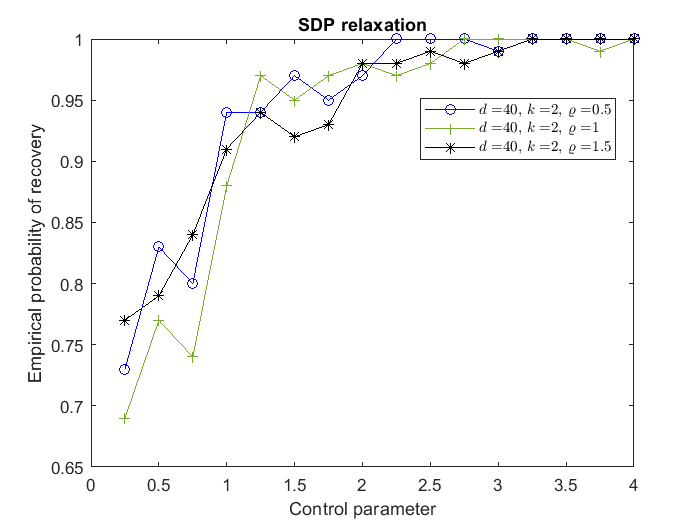
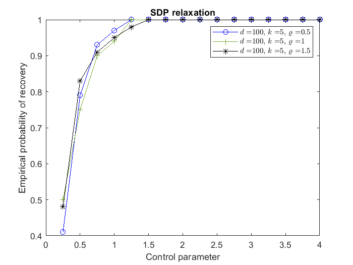
Figure 1: Performance of (3) under Model 1: empirical probability of recovery.

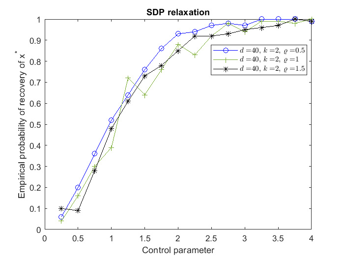
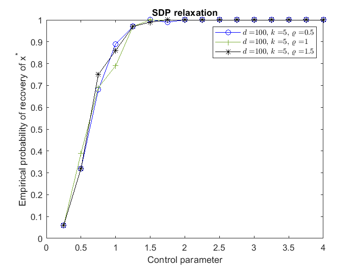
Figure 2: Performance of (3) under Model 1: empirical probability of recovery of $x^{*}$.

In this part, we show the numerical performance of (3) in the feature extraction problem under Model 1, as studied in Section 6.1.1. We assume that the entries of $M$ in Model 1 are i.i.d. standard Gaussian, and $\epsilon\sim\mathcal{N}(0_{d},\varrho^{2}I_{d})$. For simplicity, we take the first $\sigma$ entries of $z^{*}$ to be $\pm 2$, and the remaining entries to be $\pm 1$. Note that (12) indeed holds in this case. In Figure 1, we first validate Theorem 7 numerically, by plotting the empirical probability of recovery, i.e., the percentage of times (3) solves (1) over 100 instances, for each $n=\lceil cd\log(d)\rceil$, with control parameter $c$ ranging from 0.25 to 4. Note that, here, $d\log(d)$ is the dominating term in the lower bound on $n$ in Theorem 7. As discussed after Theorem 7, for small values of $n$, the recovered sparse integer vector is not necessarily the vector $x^{*}$ in the proof of Theorem 7. In Figure 2, we then plot the empirical probability of recovery of $x^{*}$, i.e., the percentage of times (3) recovers $x^{*}$ over 100 instances. The instances considered in Figure 2 are identical to those considered in Figure 1. As shown in Figures 1 and 2, both the empirical probability of recovery and the empirical probability of recovery of $x^{*}$ go to 1 as $c$ grows larger. However, the empirical probability of recovery is much closer to one also for small values of $c$.

7.3 Performance under Model 2

In this part, we show how (3) performs numerically in the integer sparse recovery problem under Model 2, as studied in Section 6.2.1. We take $c=1.2$, $c^{\prime}=1.05$, and $c^{\prime\prime}=1$ in the covariance matrix $\Sigma$, and we take $\epsilon\sim\mathcal{N}(0_{d},\varrho^{2}I_{d})$.

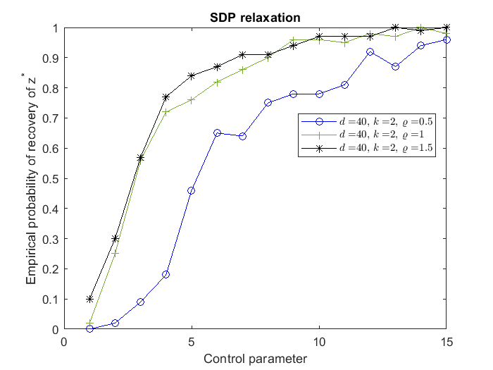
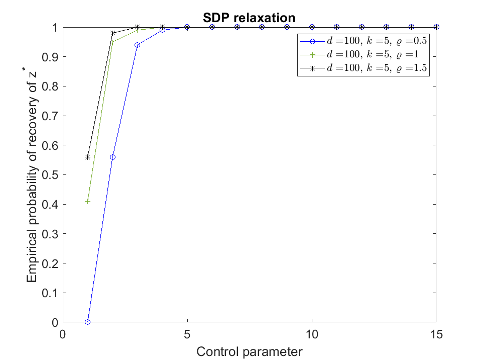
Figure 3: Performance of (3) under Model 2: empirical probability of recovery of $z^{*}$.

In Figure 3, we study the setting where $z^{*}=\begin{pmatrix}a\\ 0_{d-\sigma}\end{pmatrix}$ with $a$ uniformly drawn in $\{\pm 1\}^{\sigma}$. We plot the empirical probability of recovery of $z^{*}$ for each $n=\lceil c\varrho^{2}\sigma^{2}\log(d)\rceil$, with control parameter $c$ ranging from 1 to 15. As predicted in Theorem 9, when $c$ is large enough, the empirical probability of recovery of $z^{*}$ goes to 1 as the control parameter $c$ increases. Empirically, we also observe there is a transition to failure of recovery when the control parameter $c$ is sufficiently small.

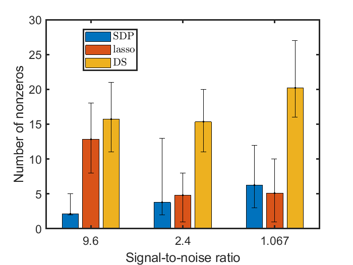
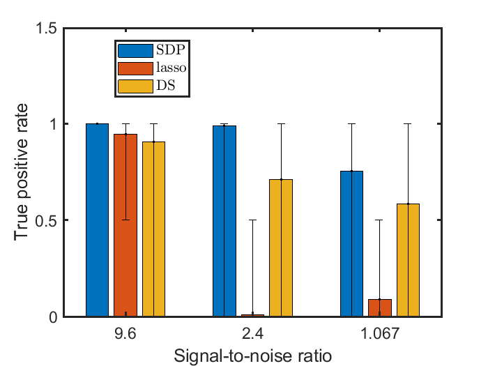
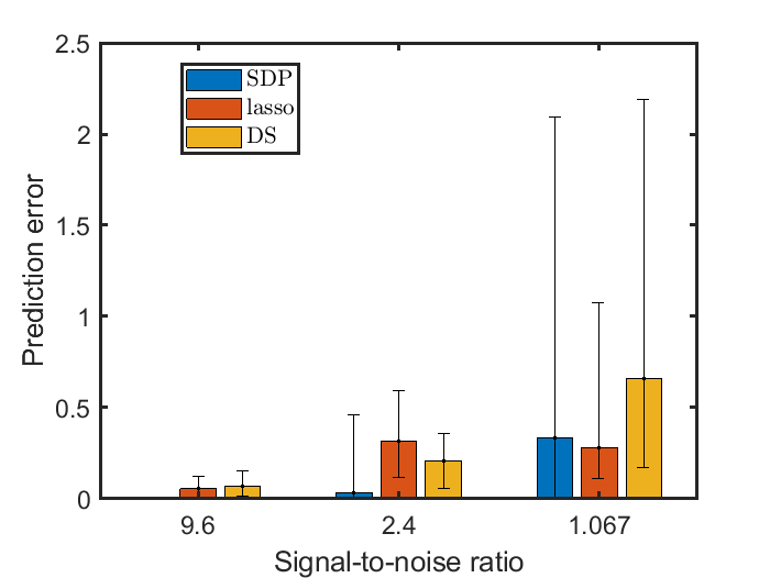
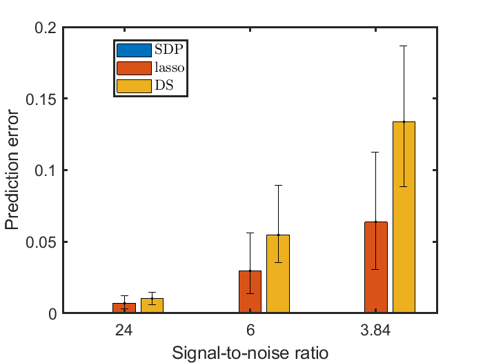
Figure 4: Performance of (3), (Lasso), (DS) under Model 2, with $d=40$, $\sigma=2$, $n=\lceil 2\sigma^{2}\log(d)\rceil=30$ in the first row, and with $d=100$, $\sigma=5$, $n=\lceil 2\sigma^{2}\log(d)\rceil=231$ in the second row. 100 instances are considered with $\varrho\in\{0.5,1,1.5\}$. The average is reported in the histogram, and the minimum and maximum in the box plot.

In Figure 4, we restrict ourselves to the setting where $z^{*}=\begin{pmatrix}1_{\sigma}\\ 0_{d-\sigma}\end{pmatrix}$, and we compare the performance of (3), (Lasso), and (DS). We are particularly interested in this setting as it is explicitly shown in [50] that Lasso is not guaranteed to perform well. This is still a high coherence model and no guarantee on the performance of Dantzig Selector is known for this model. The parameters $\lambda$ in (Lasso) and $\eta$ in (DS) are determined via a 10-fold cross-validation on a held out validation set, as suggested in [7]. We report three significant quantities for sparse recovery problems, which evaluate the quality of the solution vector $z$ returned by the algorithm. For (3), the vector $z$ that we evaluate is the vector $w^{*}$ obtained from the first column of the optimal solution $W^{*}$ to (3), by deleting its first entry equal to one. The first quantity that we report is the number of nonzeros, which is $|\operatorname{Supp}(z)|$ and measures how sparse a solution is. The second quantity that we report is the true positive rate, defined as

$$\text{true positive rate}(z):=\frac{|\operatorname{Supp}(z^{*})\cap\operatorname{Supp}(z)|}{|\operatorname{Supp}(z^{*})|}.$$

This quantity measures how well $z$ recovers the ground truth sparse vector $z^{*}$ by evaluating how much their support sets overlap. The last quantity that we report, which is suggested in [7], is known as prediction error, which is defined as

$$\text{prediction error}(z):=\frac{\left\lVert M(z-z^{*})\right\rVert_{2}^{2}}{\left\lVert Mz^{*}\right\rVert_{2}^{2}}.$$

As discussed in [7], the prediction error takes into account the correlation of features and is a meaningful measure of error for algorithms that do not have performance guarantee. We report these three quantities under different signal-to-noise ratios, i.e.,

$$\text{signal-to-noise ratio}:=\frac{\text{Var}(m_{i}^{\top}z^{*})}{\varrho^{2}}=\frac{\left\lVert\Sigma^{\frac{1}{2}}_{[d],S}z_{S}^{*}\right\rVert_{2}^{2}}{\varrho^{2}}.$$

In Figure 4, we study two sets of $(d,\sigma)$, namely, $(d,\sigma)\in\{(100,5),(40,2)\}$, with $\varrho\in\{0.5,1,1.5\}$, and we fix our choice of $n$ to be $\lceil 2\sigma^{2}\log(d)\rceil$.

In an underdetermined system ($d>n$), plotted in the first row of Figure 4, we conclude that the probability that Lasso and Dantzig Selector recover the true support $[\sigma]$ of $z^{*}$ is low, while (3) nearly always recovers the true support, even when signal-to-noise ratio is low. In an overdetermined system ($d<n$), plotted in the second row of Figure 4, the true positive rates of Lasso and Dantzig Selector dramatically improve, however they are still inferior to (3) in terms of number of nonzeros and prediction error.

We remark that, Model 2 is just one example of a high coherence model for the sparse recovery problem under which (3) works better than (Lasso) and (DS). For instance, we observe the same behavior in a model introduced in [7] (see Example 1 therein for details). For this model, several methods including Lasso, tend to give a solution with an excessively large support set, and cannot provide a satisfactory prediction error (see Fig. 4. therein for details). On the other hand, for (3), as $n$ grows, the empirical probability of recovery of $z^{*}$ tends to one, and the conditions in Theorem 8 can be satisfied.

7.4 Performance under Model 3

In this part, we study the numerical performance of (3) in the integer sparse recovery problem under Model 3, as studied in Section 6.2.2. Note that Model 3 has a low coherence when $n\geq\sigma^{2}\log(d)$. We restrict ourselves to the scenario where each entry of $M$ is i.i.d. standard Gaussian, $z^{*}=\begin{pmatrix}a\\ 0_{d-\sigma}\end{pmatrix}$ with $a$ uniformly drawn in $\{\pm 1\}^{\sigma}$, and $\epsilon\sim\mathcal{N}(0_{d},\varrho^{2}I_{d})$.

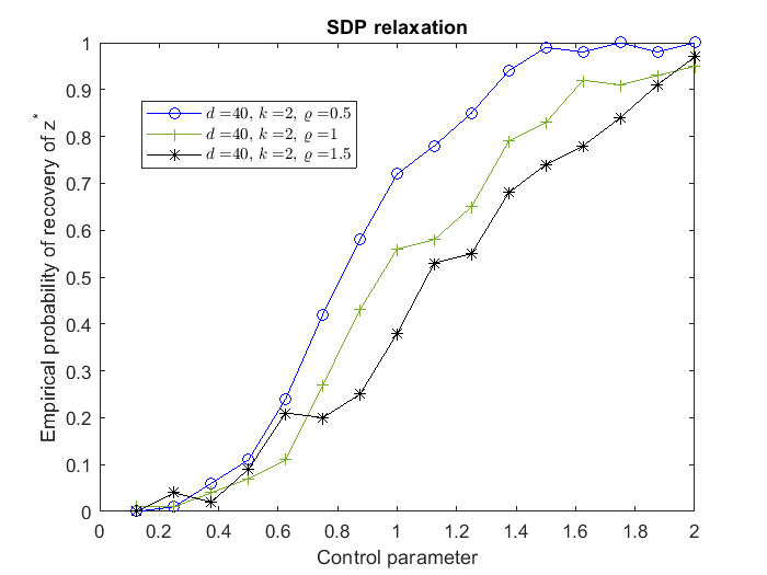
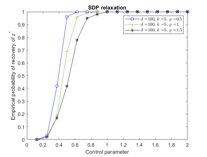
Figure 5: Performance of (3) under Model 3: empirical probability of recovery of $z^{*}$.

In Figure 5, we plot the empirical probability of recovery of $z^{*}$, for each $n=\lceil c(\sigma^{2}+\varrho^{2})\log(d)\rceil$ with control parameter $c$ ranging from $1/8$ to $2$. As predicted in Proposition 10, when $c$ grows, the probability that (3) recovers $z^{*}$ goes to 1. Empirically, we also observe that there is a transition to failure of recovery when the control parameter $c$ is sufficiently small.

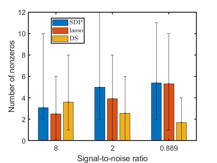
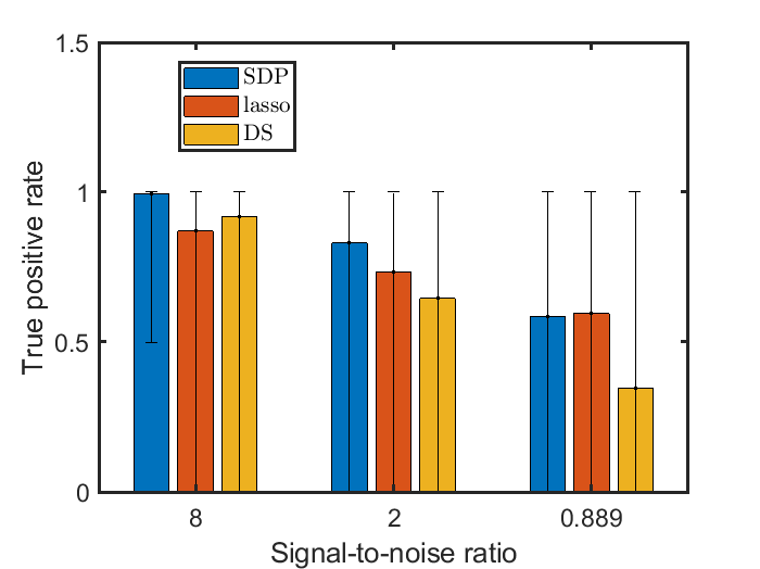
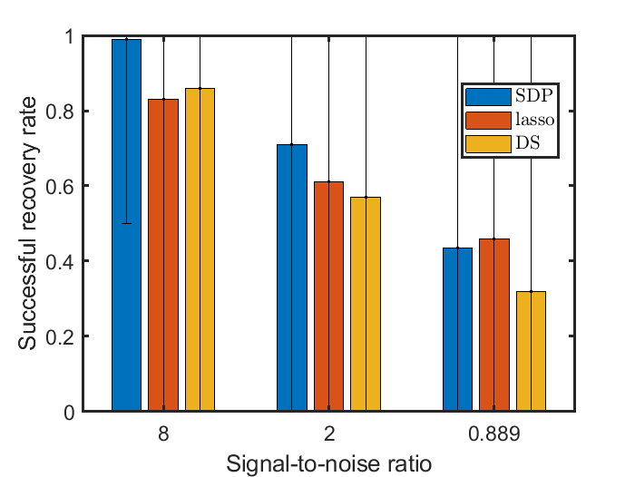
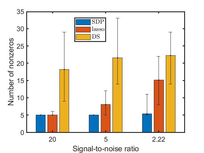
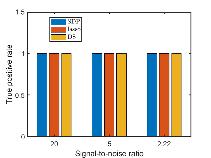
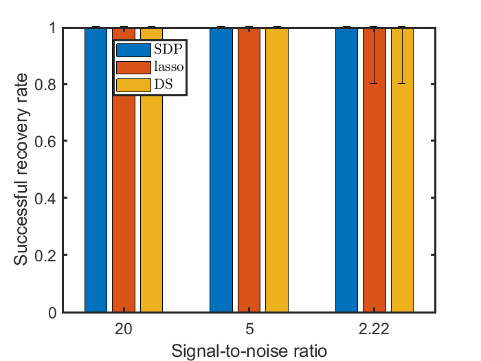
Figure 6: Performance of (3), (Lasso), and (DS) under Model 3, with $d=40$, $\sigma=2$, $n=\lceil\sigma^{2}\log(d)\rceil=15$ in the first row, and with $d=100$, $\sigma=5$, $n=\lceil\sigma^{2}\log(d)\rceil=116$ in the second row. 100 instances are considered with $\varrho\in\{0.5,1,1.5\}$. The average is reported in the histogram, and the minimum and maximum in the box plot.

In Figure 6, we compare the numerical performance of (3), (Lasso), and (DS). From [50] and [30], we know that also (Lasso) and (DS) converge to $z^{*}$, provided that we set $\lambda=2\sqrt{\log(d)/n}$ in (Lasso) and $\eta=2\varrho(5/4+\sqrt{\log(d)})$ in (DS). Hence, we set the parameters $\lambda$ and $\eta$ to these values without performing cross-validation. In Figure 6, we report three significant quantities: the first two are the number of nonzeros and the true positive rate, as defined in Section 7.3. The third one is the successful recovery rate, defined as

$$\text{successful recovery rate}(z):=\frac{|\operatorname{Supp}(z^{*})\cap S_{\max}^{\sigma}(z)|}{|\operatorname{Supp}(z^{*})|},$$

where $S_{\max}^{\sigma}(z)$ is the set indices corresponding to the top $\sigma$ entries of $z$ having largest absolute values. The reason we consider here the successful recovery rate instead of the prediction error, considered for Model 2, is that in all three algorithms $z$ converges to $z^{*}$ in Model 3. Hence, for $n$ large enough, $|z_{i}|$ is close to $0$ when $z_{i}^{*}=0$, and $|z_{j}|$ is close to one if $z^{*}_{j}=\pm 1$. Hence, we can recover $z^{*}$ by simply looking at the $\sigma$ largest entries of $|z|$. We conclude from Figure 6 that all three algorithms obtain great results in Model 3, and this is mainly due to the low coherence of the model. Since all three algorithms perform well, (Lasso) and (DS) should be preferred since they run significantly faster than (3). In particular, (3) can be solved in about one second with $d=40$ and in about one minute with $d=100$, while the other two can be solved in less than 0.1 second in both cases.

8 Proof of Theorem 2

In this section, we prove Theorem 2. To keep aligned with the notations in Section 4, throughout this section, we will keep using the same notations introduced in Algorithm 1 and Theorem 2. Moreover, we will assume the matrix $Q(c,P)=\begin{pmatrix}0&-c^{\top}\\ -c&P\end{pmatrix}$ is 0-indexed, and denote its $(i,j)$-th entry by $q_{ij}$, $0\leq i,j\leq d$. As we will see later in the proofs, $u_{0}$ is in fact a special vector, so it is worthy to distinguish it from $u_{1},u_{2},\ldots,u_{d}$, with index zero. In other sections, we will continue to assume all matrices are 1-indexed.

Recall that the problem SDP($c,P$) is defined by replacing the objective function $1/n\cdot\operatorname{tr}(A^{\top}AW)$ by $\operatorname{tr}(Q(c,P)W)$ in (3). We first show a nice property about the first column of any feasible solution to SDP($c,P$):

Proposition 2.

Consider any feasible solution $W$ to SDP($c,P$). Let the first column of $W$ be $(1,w_{x}^{\top})^{\top}$, where $w_{x}\in\mathbb{R}^{d}$. Then, $\left\lVert w_{x}\right\rVert_{1}\leq\sigma$.

Proof.

Denote $\mathcal{F}$ to be the feasible region of SDP($c,P$), we show that the optimal value of the optimization problem $\max_{W\in\mathcal{F}}\left\lVert w_{x}\right\rVert_{1}$ is exactly $\sigma$. By symmetry of $\mathcal{F}$, the problem is equivalent to $\max_{W\in\mathcal{F}}1_{d}^{\top}w_{x}$. It is clear that by taking $W^{*}:=uu^{\top}$ with $u:=(1,\sigma/d,\sigma/d,\cdots,\sigma/d)\in\mathbb{R}^{1+d}$, we attain a cost of $\sigma$ in this problem.

We conclude the proof by showing that $\sigma$ can be attained by its dual. Denote $P_{0}:=\begin{pmatrix}0&1_{d}^{\top}/2\\ 1_{d}^{\top}/2&O_{d}\end{pmatrix}$, the primal problem is then equivalent to $\max_{W\in\mathcal{F}}\operatorname{tr}(P_{0}W)$, and its dual can be derived as follows:

$$\quad\min_{\begin{subarray}{c}Y\succeq 0,\mu_{1}\in\mathbb{R},\mu_{2}\geq 0,\\ \mu_{3}\geq 0,p\geq 0_{d}\end{subarray}}\max_{W}\quad\operatorname{tr}(P_{0}W)-\mu_{1}(W_{11}-1)-\mu_{2}(\operatorname{tr}(W_{x})-\sigma)$$

$$\qquad\qquad\qquad\qquad\qquad-\mu_{3}(1_{d}^{\top}|W_{x}|1_{d}-\sigma^{2})-p^{\top}[\operatorname{diag}(W_{x})-1_{d}]+\operatorname{tr}(YW)$$

$$=\min_{\begin{subarray}{c}Y\succeq 0,\mu_{1}\in\mathbb{R},\mu_{2}\geq 0,\\ \mu_{3}\geq 0,p\geq 0_{d}\end{subarray}}\max_{W}\operatorname{tr}\left(\left(P_{0}-\mu_{1}\begin{pmatrix}1&\\ &O_{d}\end{pmatrix}-\begin{pmatrix}0&\\ &\mu_{2}I_{d}+p\end{pmatrix}+Y\right)W\right)$$

$$\qquad\qquad\qquad\qquad\qquad-\mu_{3}\operatorname{tr}(1_{d}1_{d}^{\top}|W_{x}|)+\mu_{1}+\sigma\mu_{2}+\sigma^{2}\mu_{3}+p^{\top}1_{d}$$

$$=\min_{\begin{subarray}{c}Y\succeq 0,\mu_{1}\in\mathbb{R},\mu_{2}\geq 0,\mu_{3}\geq 0\\ \left\lVert P_{0}-R(\mu_{1},\mu_{2},p)+Y\right\rVert_{\infty}\leq\mu_{3}\end{subarray}}\mu_{1}+\sigma\mu_{2}+\sigma^{2}\mu_{3}+p^{\top}1_{d},$$

where $R(\mu_{1},\mu_{2},p):=\begin{pmatrix}\mu_{1}&\\ &\mu_{2}I_{d}+p\end{pmatrix}$. It can be checked that the set of dual variables $\mu_{1}^{*}:=\sigma/2$, $\mu_{2}^{*}:=0$, $\mu_{3}^{*}:=1/(2\sigma)$, $p^{*}:=0_{d}$, and $Y^{*}:=vv^{\top}$ with $v:=\sqrt{\sigma/2}(1,1/\sigma,1/\sigma,\cdots,1/\sigma)^{\top}\in\mathbb{R}^{1+d}$ is indeed feasible to the dual problem with cost $\sigma$. ∎

The following lemma states some properties regarding some random variables that we introduce in Algorithm 1:

Lemma 3.

Consider Algorithm 1 and the variables therein. Denote $p_{0}:=1$, then:

1. ${\mathbb{E}}z_{i}z_{j}=u_{i}^{\top}u_{j}$ for those $0\leq i<j\leq d$ such that $p_{i},p_{j}>0$.

2. ${\mathbb{E}}z_{i}^{2}=\left\lVert u_{i}\right\rVert_{2}^{2}/p_{i}$ for those $1\leq i\leq d$ such that $p_{i}>0$.

3. ${\mathbb{E}}x_{i}^{2}={\mathbb{E}}|y_{i}|$ for $1\leq i\leq d$.

4. ${\mathbb{E}}x_{i}x_{j}={\mathbb{E}}y_{i}y_{j}$, for any $0\leq i<j\leq d$.

5. Define $P:=\{i\in[d]:p_{i}>0\}$, then $|P|\leq\min\{d,\sigma/C^{2}\}$.

6. For those $i,j\in P$, we have that ${\mathbb{E}}\left[\left\lvert y_{i}y_{j}-z_{i}z_{j}/T^{2}\right\rvert\right]$ is upper bounded by

   $$e^{-\frac{2C^{2}T^{2}}{9}}\left\{\frac{2\left\lVert u_{i}\right\rVert_{2}^{2}+2\left\lVert u_{j}\right\rVert_{2}^{2}}{\sqrt{2\pi}CT}+\left\lVert u_{i}\right\rVert_{2}\left\lVert u_{j}\right\rVert_{2}\left[\frac{4}{\sqrt{2\pi}}\cdot\left(\frac{2T}{3}+\frac{3}{2CT}\right)+\frac{4}{\pi}\right]\right\}$$

7. For those $j\in P$, we have that ${\mathbb{E}}\left[\left\lvert y_{0}y_{j}-z_{0}z_{j}/T^{2}\right\rvert\right]$ is upper bounded by

   $$e^{-\frac{2C^{2}T^{2}}{9}}\left\{\frac{2\left\lVert u_{j}\right\rVert_{2}^{2}}{\sqrt{2\pi}CT}+\left\lVert u_{j}\right\rVert_{2}\left[\frac{2}{\sqrt{2\pi}}\cdot\left(\frac{2T}{3}+\frac{3}{2CT}\right)+\frac{2}{\pi}\right]\right\}$$

   $$\quad+e^{-\frac{T^{2}}{2}}\left\{\frac{2}{\sqrt{2\pi}}\frac{1}{T}+\left\lVert u_{j}\right\rVert_{2}\cdot\left[\frac{2}{\sqrt{2\pi}}\left(T+\frac{2}{T}\right)+\frac{1}{\pi}\right]\right\}$$

Proof.

3A, 3B, and 3C follow from direct calculation. We start with 3D. We first consider the case $i=0$. We observe that the conditional probability ${\mathbb{E}}[x_{0}x_{j}|y_{0},y_{j}]$ is exactly $y_{0}y_{j}$. Indeed,

$${\mathbb{E}}[x_{0}x_{j}|y_{0},y_{j}]=\left(1\cdot\frac{1+y_{0}}{2}\right)\cdot\operatorname{sign}(y_{j})|y_{j}|+\left(-1\cdot\frac{1-y_{0}}{2}\right)\cdot\operatorname{sign}(y_{j})|y_{j}|=y_{0}y_{j},$$

and then by law of total expectation we are done. Then, we assume that $i\geq 1$, and we see that

$${\mathbb{E}}[x_{i}x_{j}|y_{i},y_{j}]=\left(\operatorname{sign}(y_{i})\cdot|y_{i}|\right)\cdot\left(\operatorname{sign}(y_{j})\cdot|y_{j}|\right)=y_{i}y_{j}.$$

By law of total expectation, we again obtain the desired result.

To show 3E, one only need to observe that

$$\sigma\geq\sum_{i=1}^{d}\left\lVert u_{i}\right\rVert_{2}^{2}\geq\sum_{i\in P}\left\lVert u_{i}\right\rVert_{2}^{2}\geq C^{2}|P|.$$

Finally, we show 3F and 3G. The proof ideas are almost identical to that of Lemma 2 in [12], but for the completeness of the paper, we leave a proof here. We define the random event $S:=\{g:|z_{i}|\leq 1,|z_{j}|\leq 1\}$, thus ${\mathbb{E}}[|z_{i}z_{j}/T^{2}-y_{i}y_{j}|;S]=0$. This implies that we only need to upper bound the difference $|z_{i}z_{j}/T^{2}-y_{i}y_{j}|$ when $|z_{i}|>1$ or $|z_{j}|>1$. Next, due to rotational symmetry of $g$, we can assume WLOG that $u_{i}=\left\lVert u_{i}\right\rVert_{2}\cdot(1,0,\ldots,0)^{\top}$ and $u_{j}=\left\lVert u_{j}\right\rVert_{2}\cdot(a,b,0,\ldots,0)^{\top}$ with $a^{2}+b^{2}=1$, without changing distributions of $z_{i}$ and $z_{j}$. We first define $B:=\{g:z_{i}>1\}$, and denote $Z\sim\mathcal{N}(0,1)$ to be a standard Gaussian variable. Since $g^{\top}u$ has the same distribution as $\left\lVert u\right\rVert_{2}Z$, we see that for $i\geq 1$,

$$\quad{\mathbb{E}}[|y_{i}y_{j}|;B]\leq{\mathbb{E}}[1;B]={\mathbb{P}}(B)={\mathbb{P}}\left(z_{i}>T,\tilde{u}_{i}=\frac{u_{i}}{p_{i}}\right)$$

$$=p_{i}{\mathbb{P}}\left(\frac{\left\lVert u_{i}\right\rVert_{2}}{p_{i}}Z>T\right)=p_{i}{\mathbb{P}}\left(Z>\frac{p_{i}}{\left\lVert u_{i}\right\rVert_{2}}T\right)\leq p_{i}{\mathbb{P}}\left(Z>\frac{2}{3}C\cdot T\right)$$

$$=p_{i}\int_{\frac{2}{3}CT}^{\infty}\frac{1}{\sqrt{2\pi}}e^{-\frac{x^{2}}{2}}\textup{d}x<p_{i}\cdot\frac{1}{\sqrt{2\pi}}\frac{1}{\left(\frac{2}{3}CT\right)}e^{-\frac{2C^{2}T^{2}}{9}}=\frac{\left\lVert u_{i}\right\rVert_{2}^{2}}{\sqrt{2\pi}}\frac{1}{CT}e^{-\frac{2C^{2}T^{2}}{9}}$$

where we use the fact that $\int_{t}^{+\infty}e^{-x^{2}/2}\textup{d}x<1/t\cdot e^{-t^{2}/2}$ in the last line. Note that the above bound is similar when $i=0$. We see that

$$\quad{\mathbb{E}}[|y_{0}y_{j}|;B]\leq{\mathbb{E}}[1;B]={\mathbb{P}}(B)={\mathbb{P}}\left(z_{0}>T\right)={\mathbb{P}}\left(g^{\top}u_{0}>T\right)$$

$$={\mathbb{P}}\left(Z>T\right)=\int_{T}^{\infty}\frac{1}{\sqrt{2\pi}}e^{-\frac{x^{2}}{2}}\textup{d}x<\frac{1}{\sqrt{2\pi}}\frac{1}{T}e^{-\frac{T^{2}}{2}}$$

Then, we calculate ${\mathbb{E}}[|z_{i}z_{j}|;B]$. Since ${\mathbb{E}}[|z_{i}z_{j}|;B]={\mathbb{E}}{\mathbb{E}}[|z_{i}z_{j}|\mathds{1}_{B}|\tilde{u}_{i},\tilde{u}_{j}]$, we calculate the conditional expectation first. We see that

$${\mathbb{E}}\left[|z_{i}z_{j}|\mathds{1}_{B}\Bigg{|}\tilde{u}_{i}=\frac{u_{i}}{p_{i}},\tilde{u}_{j}=\frac{u_{j}}{p_{j}}\right]=\frac{\left\lVert u_{i}\right\rVert_{2}\left\lVert u_{j}\right\rVert_{2}}{2\pi p_{i}p_{j}}\int_{-\infty}^{+\infty}\int_{\frac{p_{i}T}{\left\lVert u_{i}\right\rVert_{2}}}^{+\infty}|s(as+bt)|e^{-\frac{s^{2}}{2}}e^{-\frac{t^{2}}{2}}\textup{d}s\textup{d}t.$$

Since

$$\quad\int_{\frac{p_{i}T}{\left\lVert u_{i}\right\rVert_{2}}}^{+\infty}s^{2}e^{-\frac{s^{2}}{2}}\textup{d}s=-se^{-\frac{s^{2}}{2}}\Bigg{|}_{\frac{p_{i}T}{\left\lVert u_{i}\right\rVert_{2}}}^{+\infty}+\int_{\frac{p_{i}T}{\left\lVert u_{i}\right\rVert_{2}}}^{+\infty}e^{-\frac{s^{2}}{2}}\textup{d}s$$

$$<\frac{p_{i}T}{\left\lVert u_{i}\right\rVert_{2}}e^{-\frac{p_{i}^{2}T^{2}}{2\left\lVert u_{i}\right\rVert_{2}^{2}}}+\frac{1}{\left(\frac{p_{i}}{\left\lVert u_{i}\right\rVert_{2}}T\right)}e^{-\frac{p_{i}^{2}T^{2}}{2\left\lVert u_{i}\right\rVert_{2}^{2}}}\leq\frac{2T}{3}e^{-\frac{2C^{2}T^{2}}{9}}+\frac{3}{2CT}e^{-\frac{2C^{2}T^{2}}{9}}$$

and

$$\int_{\frac{p_{i}T}{\left\lVert u_{i}\right\rVert_{2}}}^{+\infty}|s|e^{-\frac{s^{2}}{2}}\textup{d}s=e^{-\frac{p_{i}^{2}T^{2}}{2\left\lVert u_{i}\right\rVert_{2}^{2}}}\leq e^{-\frac{2C^{2}T^{2}}{9}},$$

we obtain that

$${\mathbb{E}}\left[|z_{i}z_{j}|\mathds{1}_{B}\right] \leq\left\lVert u_{i}\right\rVert_{2}\left\lVert u_{j}\right\rVert_{2}\cdot e^{-\frac{2C^{2}T^{2}}{9}}\cdot\left[\frac{1}{\sqrt{2\pi}}\cdot\left(\frac{2T}{3}+\frac{3}{2CT}\right)+\frac{1}{\pi}\right]$$

Note that for $i=0$, the calculation is similar, and one can obtain that

$${\mathbb{E}}\left[|z_{0}z_{j}|\mathds{1}_{B}\Bigg{|}\tilde{u}_{j}=\frac{u_{j}}{p_{j}}\right] =\frac{\left\lVert u_{j}\right\rVert_{2}}{p_{j}}\int_{-\infty}^{+\infty}\int_{T}^{+\infty}|s(as+bt)|\frac{1}{2\pi}e^{-\frac{s^{2}}{2}}e^{-\frac{t^{2}}{2}}\textup{d}s\textup{d}t$$

$$\leq\frac{\left\lVert u_{j}\right\rVert_{2}}{p_{j}}\cdot\left[\frac{1}{\sqrt{2\pi}}\left(T+\frac{1}{T}\right)e^{-\frac{T^{2}}{2}}+\frac{1}{\pi}e^{-\frac{T^{2}}{2}}\right],$$

and hence

$${\mathbb{E}}\left[|z_{0}z_{j}|\mathds{1}_{B}\right]\leq\left\lVert u_{0}\right\rVert_{2}\left\lVert u_{j}\right\rVert_{2}\cdot\left[\frac{1}{\sqrt{2\pi}}\left(T+\frac{1}{T}\right)+\frac{1}{\pi}\right]e^{-\frac{T^{2}}{2}}$$

By symmetry, similar upper bounds hold for random events $\{g:z_{i}<-1\}$, $\{g:z_{j}>1\}$, and $\{g:z_{j}<-1\}$. Therefore, we obtain 3F and 3G. ∎

We are now ready to prove Theorem 2:

Proof of Theorem 2.

We first show the approximation gap. The second inequality is due to relaxation and $\epsilon$-optimality, and we only need to show the first. We denote $U:=(u_{0},u_{1},\ldots,u_{d})=\sqrt{W^{*}}$, as in Algorithm 1. We observe that $\bar{x}^{\top}P\bar{x}-2c^{\top}\bar{x}=\sum_{i,j=0}^{d}q_{ij}\bar{x}_{i}\bar{x}_{j}$, and $\operatorname{tr}(Q(c,P)W^{*})=\sum_{i,j=0}^{d}q_{ij}u_{i}^{\top}u_{j}$. We will split the proof into two parts:

1. (Non-diagonal entries, i.e., $i<j$) We first assume $p_{i},p_{j}>0$, where $p_{i}$’s are defined in Algorithm 1. By 3A, 3D, and the fact that $\bar{x}$ differs $x$ only by possibly flipping a sign in Algorithm 1, we observe that

   $$\frac{1}{T^{2}}\cdot q_{ij}u_{i}^{\top}u_{j} =q_{ij}{\mathbb{E}}y_{i}y_{j}+q_{ij}\left(\frac{1}{T^{2}}{\mathbb{E}}z_{i}z_{j}-{\mathbb{E}}y_{i}y_{j}\right)$$

   $$=q_{ij}{\mathbb{E}}\bar{x}_{i}\bar{x}_{j}+q_{ij}\left(\frac{1}{T^{2}}{\mathbb{E}}z_{i}z_{j}-{\mathbb{E}}y_{i}y_{j}\right)$$

   $$\geq q_{ij}{\mathbb{E}}\bar{x}_{i}\bar{x}_{j}-|q_{ij}|\cdot{\mathbb{E}}\left[\Bigg{|}y_{i}y_{j}-z_{i}z_{j}\cdot\frac{1}{T^{2}}\Bigg{|}\right].$$

   For the case where, WLOG, $p_{i}=0$. By the definition of $p_{i}$ in Algorithm 1, it must be the case $\left\lVert u_{i}\right\rVert_{2}\leq C$. Therefore, we obtain a trivial bound (note that ${\mathbb{E}}\bar{x}_{i}\bar{x}_{j}=0$)

   $$\frac{1}{T^{2}}\cdot q_{ij}u_{i}^{\top}u_{j}\geq q_{ij}{\mathbb{E}}\bar{x}_{i}\bar{x}_{j}-\frac{1}{T^{2}}\cdot|q_{ij}|\cdot|u_{i}^{\top}u_{j}|.$$

2. (Diagonal entries, i.e., $i=j$) We first study the case $p_{i}>0$ ($i\geq 1$). By 3B, 3C, and the facts that $q_{ii}\geq 0$, $\left\lVert u_{i}\right\rVert_{2}\geq C$, and $p_{i}=2/3\cdot\left\lVert u_{i}\right\rVert_{2}^{2}$, we see that

   $$q_{ii}{\mathbb{E}}\bar{x}_{i}^{2} =q_{ii}{\mathbb{E}}|y_{i}|\leq q_{ii}\sqrt{{\mathbb{E}}|y_{i}|^{2}}\leq q_{ii}\sqrt{{\mathbb{E}}\frac{1}{T^{2}}|z_{i}|^{2}}=\frac{q_{ii}}{T\sqrt{p_{i}}}\left\lVert u_{i}\right\rVert_{2}=\frac{\sqrt{3}q_{ii}}{\sqrt{2}T}$$

   $$=\frac{q_{ii}}{T^{2}}u_{i}^{\top}u_{i}+q_{ii}\left(\frac{\sqrt{3}}{\sqrt{2}T}-\frac{1}{T^{2}}u_{i}^{\top}u_{i}\right)$$

   For the case $p_{i}=0$, we again use the trivial inequality

   $$\frac{1}{T^{2}}\cdot q_{ii}u_{i}^{\top}u_{i}\geq q_{ii}{\mathbb{E}}\bar{x}_{i}^{2}-\frac{1}{T^{2}}\cdot q_{ii}\cdot u_{i}^{\top}u_{i}.$$

Denote the set $P:=\{i\in[d]:p_{i}>0\}$ the same as in 3E, and define $g(C,T):=1/\sqrt{2\pi}\cdot\left(2T/3+3/(2T)\right)+1/\pi$. Putting (i), (ii), 3F, and 3G together, we see that $\operatorname{tr}(Q(c,P)W^{*})/T^{2}$ is lower bounded by

$$\quad\sum_{i,j=0}^{d}q_{ij}{\mathbb{E}}\bar{x}_{i}\bar{x}_{j}-\sum_{\begin{subarray}{c}i\neq j,\\ i,j\in P\end{subarray}}|q_{ij}|e^{-\frac{2C^{2}T^{2}}{9}}\left\{\frac{2\left\lVert u_{i}\right\rVert_{2}^{2}+2\left\lVert u_{j}\right\rVert_{2}^{2}}{\sqrt{2\pi}CT}+4g(C,T)\left\lVert u_{i}\right\rVert_{2}\left\lVert u_{j}\right\rVert_{2}\right\}$$

$$\quad-2\sum_{j\in P}|q_{0j}|\Bigg{\{}e^{-\frac{2C^{2}T^{2}}{9}}\left\{\frac{2\left\lVert u_{j}\right\rVert_{2}^{2}}{\sqrt{2\pi}CT}+2g(C,T)\left\lVert u_{j}\right\rVert_{2}\right\}$$

$$\quad+e^{-\frac{T^{2}}{2}}\left\{\frac{2}{\sqrt{2\pi}}\frac{1}{T}+\left\lVert u_{j}\right\rVert_{2}\cdot\left[\frac{2}{\sqrt{2\pi}}\left(T+\frac{2}{T}\right)+\frac{1}{\pi}\right]\right\}\Bigg{\}}$$

$$\quad-\frac{1}{T^{2}}\sum_{\begin{subarray}{c}(i,j)\not\in P\times P,\\ 0\leq i,j\leq d,(i,j)\neq(0,0)\end{subarray}}|q_{ij}|\cdot|u_{i}^{\top}u_{j}|-\sum_{i\in P}q_{ii}\left\lvert\frac{\sqrt{3}}{\sqrt{2}T}-\frac{1}{T^{2}}u_{i}^{\top}u_{i}\right\rvert$$

$$\geq\sum_{i,j=0}^{d}q_{ij}{\mathbb{E}}\bar{x}_{i}\bar{x}_{j}-B\cdot e^{-\frac{2C^{2}T^{2}}{9}}\left\{\frac{4\sigma\min\{d,\sigma/C^{2}\}}{\sqrt{2\pi}CT}+\frac{4\sigma}{\sqrt{2\pi}CT}+4g(C,T)\left(\sigma+1\right)\right\}$$

$$\quad-B\cdot e^{-\frac{T^{2}}{2}}\left\{\frac{2|P|}{\sqrt{2\pi}T}+\frac{\sigma}{C}\cdot\left[\frac{2}{\sqrt{2\pi}}\left(T+\frac{2}{T}\right)+\frac{1}{\pi}\right]\right\}-\frac{1}{T^{2}}B(3\sigma+\sigma^{2})-\frac{\sqrt{3}B}{\sqrt{2}T}|P|,$$

where we use Hölder’s inequality with $(\infty,1)$-norm, together with the following facts:

• $\sum_{i=1}^{d}\left\lVert u_{i}\right\rVert_{2}^{2}=\operatorname{tr}(W_{x}^{*})\leq\sigma$, $\left\lVert u_{0}\right\rVert_{2}^{2}=W_{11}^{*}=1$,

• $\sum_{i\in P}\left\lVert u_{i}\right\rVert_{2}\leq\sum_{i\in P}\left\lVert u_{i}\right\rVert_{2}^{2}/C\leq\sigma/C$,

• $\sum_{0\leq i,j\leq d}\left\lVert u_{i}\right\rVert_{2}\left\lVert u_{j}\right\rVert_{2}\leq\sum_{i=0}^{d}\left\lVert u_{i}\right\rVert_{2}^{2}\leq\sigma+1$,

• $\sum_{0\leq i,j\leq d,(i,j)\neq(0,0)}|u_{i}^{\top}u_{j}|\leq 2\sum_{i=1}^{d}|u_{0}^{\top}u_{i}|+\sum_{i,j=1}^{d}|u_{i}^{\top}u_{j}|\leq 2\sigma+\sigma^{2}$, where we use Proposition 2 and $1_{d}^{\top}|W_{x}^{*}|1_{d}\leq\sigma^{2}$ in the last inequality.

Lastly, by 3E we obtain our desired inequality.

To conclude the proof, we remains to show that $\bar{x}$ is feasible to (4) with high probability. we only need to show that $\left\lVert\bar{x}\right\rVert_{0}\leq\sigma$ holds with probability at least $1-\exp\{-c\sigma\}$ for some (absolute) constant $c>0$. Since ${\mathbb{E}}\left\lVert\bar{x}\right\rVert_{0}\leq\sum_{i=1}^{d}p_{i}\leq 2/3\cdot\sigma$, by multiplicative Chernoff bound equipped with an upper bound for the expectation (see, e.g., Theorem 4.4 and the remark after Corollary 4.6 in [35]), we have

$${\mathbb{P}}\left(\left\lVert\bar{x}\right\rVert_{0}\geq\sigma\right)\leq{\mathbb{P}}\left(\left\lVert\bar{x}\right\rVert_{0}\geq\left(1+\frac{1}{2}\right)\cdot\frac{2}{3}\sigma\right)\leq e^{-\frac{\sigma}{18}}.$$

∎

9 Proofs of Theorems 3 and 4

In this section, we prove Theorem 3 and Theorem 4, stated in Section 5.

We first prove Lemma 1, and then we use it to prove prove Theorem 3 in Section 9.1 and Theorem 4 in Section 9.2. To show Lemma 1, we need two lemmas.

Lemma 4 ([22], Section 5).

Let $D=\operatorname{diag}(d_{i})$ be a diagonal matrix of order $n$, and let $C=D+auu^{\top}$ with $a<0$ and $u$ being an $n$-vector. Denote the eigenvalues of $C$ by $\lambda_{1},\lambda_{2},\cdots,\lambda_{n}$ and assume $\lambda_{i}\leq\lambda_{i+1}$, $d_{i}\leq d_{i+1}$. We have $d_{1}+a\left\lVert u\right\rVert_{2}^{2}\leq\lambda_{1}\leq d_{1}$, and $d_{i-1}\leq\lambda_{i}\leq d_{i}$ for $i\geq 2$.

Lemma 5 ([8], Appendix A.5.5).

Let $P$ be a symmetric matrix written as a $2\times 2$ block matrix $P=\begin{pmatrix}P_{11}&P_{12}\\ P_{12}^{\top}&P_{22}\end{pmatrix}$. The following are equivalent:

1. $P\succeq 0$.

2. $P_{11}\succeq 0$, $(I-P_{11}P_{11}^{\dagger})P_{12}=O$, and $P_{22}\succeq P_{12}^{\top}P_{11}^{\dagger}P_{12}$.

We are now ready to prove Lemma 1.

Proof of Lemma 1.

We divide the proof into three steps. In Step A, we show $p^{*}\geq 0_{d}$, $\lambda_{2}(H_{S,S})\geq\delta$, and $H_{S,S}\succeq 0$. In Step B, we show that if in addition, 1A - 1D hold, then $W^{*}$ is optimal to (3). In Step C, we show that if furthermore $\lambda_{2}(H)>0$ holds, then $W^{*}$ is the unique optimal solution to (3).

Step A. We first show $p^{*}\geq 0_{d}$. Since $p_{S^{c}}^{*}=0_{d-\sigma}$, it suffices to prove $p_{S}^{*}\geq 0_{\sigma}$. We have

$$\min_{i\in S}p_{i}^{*} =-\sigma\mu_{3}^{*}-\mu_{2}^{*}+\min_{i\in S}\big{[}(-\frac{1}{n}(M^{\top}M)_{S,S}x_{S}^{*})_{i}-y_{i}^{*}\big{]}/x_{i}^{*}$$ (14)

$$\stackrel{{\scriptstyle\text{\eqref{choice of mu3}}}}{{=}}-\lambda_{\min}\big{(}\frac{1}{n}(M^{\top}M)_{S,S}\big{)}+\delta-\mu_{2}^{*}\geq 0,$$

where the last inequality is due to (5). Next, we show $\lambda_{2}(H_{S,S})\geq\delta$. To see this, (3) gives

$$H_{S,S} =\frac{1}{n}(M^{\top}M)_{S,S}+\mu_{3}^{*}x^{*}_{S}(x^{*}_{S})^{\top}+\operatorname{diag}(p_{S}^{*}+\mu_{2}^{*}1_{\sigma})-\frac{1}{Y_{11}^{*}}y_{S}^{*}(y_{S}^{*})^{\top}.$$

By (4), $x_{S}^{*}$ is an eigenvector of $H_{S,S}$ corresponding to the zero eigenvalue. Therefore, to show $\lambda_{2}(H_{S,S})\geq\delta$, it is sufficient to show that for any unit vector $a\in\operatorname{Span}1(\{x_{S}^{*}\})^{\perp}$, we have $a^{\top}H_{S,S}a\geq\delta$. We obtain

$$a^{\top}H_{S,S}a =a^{\top}\Big{(}\frac{1}{n}(M^{\top}M)_{S,S}+\mu_{3}^{*}x_{S}^{*}(x_{S}^{*})^{\top}+\operatorname{diag}(p_{S}^{*}+\mu_{2}^{*}1_{\sigma})-\frac{1}{Y_{11}^{*}}y_{S}^{*}(y_{S}^{*})^{\top}\Big{)}a$$

$$=a^{\top}\Big{(}\frac{1}{n}(M^{\top}M)_{S,S}+\operatorname{diag}(p_{S}^{*}+\mu_{2}^{*}1_{\sigma})-\frac{1}{Y_{11}^{*}}y_{S}^{*}(y_{S}^{*})^{\top}\Big{)}a.$$

We then define the following two auxiliary matrices:

$$R :=\frac{1}{n}(M^{\top}M)_{S,S}+\mu_{2}^{*}I_{\sigma}+\operatorname{diag}(p_{S}^{*})-\frac{1}{Y_{11}^{*}}y_{S}^{*}(y_{S}^{*})^{\top},$$

$$P :=\frac{1}{n}(M^{\top}M)_{S,S}+\mu_{2}^{*}I_{\sigma}+\operatorname{diag}(p_{S}^{*}).$$

To prove $a^{\top}H_{S,S}a\geq\delta$, it is sufficient to show $\lambda_{\min}(P)\geq\delta$. Indeed, by Lemma 4, we see $\lambda_{2}(R)\geq\lambda_{\min}(P)\geq\delta$. From (4), $x_{S}^{*}$ is an eigenvector of $R$ corresponding to eigenvalue $-\sigma\mu_{3}^{*}\leq 0$, so it is an eigenvector corresponding to the smallest eigenvalue of $R$, which then implies $a^{\top}H_{S,S}a=a^{\top}Ra\geq\delta$. We now check $\lambda_{\min}(P)\geq\delta$. Recall again $\min_{i\in S}p_{i}^{*}=-\lambda_{\min}\big{(}\frac{1}{n}(M^{\top}M)_{S,S}\big{)}+\delta-\mu_{2}^{*}$ by (14). We have

$$P=\frac{1}{n}(M^{\top}M)_{S,S}+\mu_{2}^{*}I_{\sigma}+\operatorname{diag}(p_{S}^{*})\succeq\Big{(}\lambda_{\min}\big{(}\frac{1}{n}(M^{\top}M)_{S,S}\big{)}+\mu_{2}^{*}+\min_{i\in S}p_{i}^{*}\Big{)}I_{\sigma}=\delta I_{\sigma}.$$

This concludes the proof that $\lambda_{\min}(P)\geq\delta$, and therefore $\lambda_{2}(H_{S,S})\geq\delta$.

Finally, $H_{S,S}\succeq 0$ follows easily if one observes that $\lambda_{\min}(H_{S,S})=0$. Indeed, direct calculation and (4) gives $H_{S,S}x_{S}^{*}=0_{\sigma}$, which gives our desired property.

Step B. In this part, we show $W^{*}$ is optimal by checking (KKT-1) - (KKT-3). We first show that $H\succeq 0$. From Lemma 5, it suffices to show the following three facts: (i) $H_{S,S}\succeq 0$, (ii) $(I_{\sigma}-H_{S,S}H_{S,S}^{\dagger})H_{S,S^{c}}=O_{\sigma\times(d-\sigma)}$, and (iii) $H_{S^{c},S^{c}}\succeq H_{S^{c},S}H_{S,S}^{\dagger}H_{S^{c},S}^{\top}$. Note that (i) holds by part (a) and (iii) holds by 1A, so it remains to show (ii). We see

$$(I_{\sigma}-H_{S,S}H_{S,S}^{\dagger})H_{S,S^{c}}=\frac{1}{\sigma}x_{S}^{*}(x_{S}^{*})^{\top}H_{S,S^{c}}\stackrel{{\scriptstyle\ref{condition 2.2}}}{{=}}\frac{1}{\sigma}x_{S}^{*}0_{d-\sigma}^{\top}=O_{\sigma\times(d-\sigma)},$$

where we have used the facts $\lambda_{2}(H_{S,S})\geq\delta>0$ from part (a) and $H_{S,S}x_{S}^{*}=0_{\sigma}$ in the first equality.

We define $Y^{*}:=\begin{pmatrix}Y_{11}^{*}&(y^{*})^{\top}\\ y^{*}&Y_{x}^{*}\end{pmatrix}$ and $\mu_{1}^{*}:=Y_{11}^{*}-1/n\cdot b^{\top}b$. Observe that $Y^{*}\succeq 0$ again by Lemma 5, due to the facts $H\succeq 0$ and $Y_{11}^{*}>0$. (KKT-1) is equivalent to

$$-\mu_{3}^{*}x_{S}^{*}(x_{S}^{*})^{\top} =\left[\frac{1}{n}M^{\top}M-Y_{x}^{*}+\operatorname{diag}(p^{*}+\mu_{2}^{*}1_{d})\right]_{S,S},$$ (15)

$$\mu_{3}^{*}1_{d}1_{d}^{\top} \geq\left|\frac{1}{n}M^{\top}M-Y^{*}_{x}+\operatorname{diag}(p^{*}+\mu_{2}^{*}1_{d})\right|.$$ (16)

We see that (15) coincides with (3), and (16) is implied by (3), the fact that $p_{S^{c}}^{*}=0_{d-\sigma}$, 1C, and 1D. (KKT-2) and (KKT-3) hold clearly by definition.

Step C. Finally, we show that $W^{*}$ is the unique optimal solution if we additionally assume $\lambda_{2}(H)>0$. First, note that $\lambda_{2}(H)>0$ implies $\lambda_{2}(Y^{*})>0$ due to the fact that

$$Y^{*}=\begin{pmatrix}Y_{11}^{*}&(y^{*})^{\top}\\ y^{*}&Y_{x}^{*}\end{pmatrix}=\begin{pmatrix}1&\\ \frac{1}{Y_{11}^{*}}y^{*}&I_{d}\end{pmatrix}\begin{pmatrix}Y_{11}^{*}&\\ &Y_{x}^{*}-\frac{1}{Y_{11}^{*}}y^{*}(y^{*})^{\top}\end{pmatrix}\begin{pmatrix}1&\\ \frac{1}{Y_{11}^{*}}y^{*}&I_{d}\end{pmatrix}^{\top}.$$

We define the Lagrangian function $\mathcal{L}:\mathbb{R}^{(1+d)\times(1+d)}\to\mathbb{R}$ as follows:

$$\mathcal{L}(W) :=\frac{1}{n}\operatorname{tr}(A^{\top}AW)-\operatorname{tr}(Y^{*}W)+\mu_{1}^{*}(W_{11}-1)$$

$$\qquad+\mu_{2}^{*}(\operatorname{tr}(W_{x})-\sigma)+\mu_{3}^{*}(1_{d}^{\top}\left\lvert W_{x}\right\rvert 1_{d}-\sigma^{2})+\operatorname{tr}(\operatorname{diag}(p^{*})(W_{x}-I)).$$

Then, for any optimal solution $W_{0}$ to (3), we show $W^{*}=W_{0}$. It is clear that

$$\frac{1}{n}\operatorname{tr}(A^{\top}AW_{0})\geq\mathcal{L}(W_{0})\geq\mathcal{L}(W^{*})=\frac{1}{n}\operatorname{tr}(A^{\top}AW^{*}),$$

where the second inequality is due to (KKT-1), which states that $O_{1+d}$ lies in the subdifferential of $\mathcal{L}(W^{*})$. By the optimality of $W_{0}$, it is clear that, from the second term $-\operatorname{tr}(Y^{*}W_{0})$ to the last term $\operatorname{tr}(\operatorname{diag}(p^{*})((W_{0})_{x}-I))$ in $\mathcal{L}(W_{0})$, are all zero, as they are always non-positive. In particular, $0=\operatorname{tr}(Y^{*}W^{*})=\operatorname{tr}(Y^{*}W_{0})$ holds. This implies that $W_{0}$ must be a scaling of $W^{*}$ since $\lambda_{2}(Y^{*})>0$. Again by optimality of $W_{0}$, we see $W_{0}=W^{*}$.

∎

In the remainder of the section we prove Theorems 3 and 4. We start with a useful lemma, which introduces the Schur complement of a positive semidefinite matrix. This result follows from Lemma 5.

Lemma 6.

For a positive semidefinite matrix $H\in\mathbb{R}^{d\times d}$, and a set of indices $S\subseteq[d]$. Denote $P_{1}:=\begin{pmatrix}I_{\sigma}&\\ H_{S,S^{c}}^{\top}H_{S,S}^{\dagger}&I_{d-\sigma}\end{pmatrix}$, we have

$$\begin{pmatrix}H_{S,S}&H_{S,S^{c}}\\ H_{S,S^{c}}^{\top}&H_{S^{c},S^{c}}\end{pmatrix} =P_{1}\cdot\begin{pmatrix}H_{S,S}&\\ &H_{S^{c},S^{c}}-H_{S,S^{c}}^{\top}H_{S,S}^{\dagger}H_{S,S^{c}}\end{pmatrix}\cdot P_{1}^{\top}.$$

9.1 Proof of Theorem 3

In this proof we intend to use Lemma 1, thus we check that all assumptions in Lemma 1 are satisfied. In particular, we take $(Y_{x}^{*})_{S,S}$ as per (3), $p_{S}^{*}$ as per (4), and $p^{*}_{S^{c}}=0_{d-\sigma}$, as in the statement of Lemma 1. Note that since $Y_{x}^{*}$ is not completely determined, we also need to define its missing parts, i.e., its $(S^{c},S)$ and $(S^{c},S^{c})$ blocks. For brevity, we denote $H^{0}:=I_{\sigma}-x_{S}^{*}(x_{S}^{*})^{\top}/\sigma$ and $P:=(M^{\top}M)_{S,S^{c}}/n-y^{*}_{S}(y^{*}_{S^{c}})^{\top}/Y_{11}^{*}$. We take

$$(Y_{x}^{*})_{S^{c},S} :=\frac{1}{n}(M^{\top}M)_{S^{c},S}-\left[\frac{1}{n\sigma}(M^{\top}M)_{S^{c},S}x_{S}^{*}-\frac{1}{Y_{11}^{*}\sigma}y^{*}_{S^{c}}(y^{*}_{S})^{\top}x_{S}^{*}\right](x_{S}^{*})^{\top},$$ (17)

$$(Y_{x}^{*})_{S^{c},S^{c}} :=\Theta_{1}+\nu I_{d-\sigma}+\frac{1}{Y_{11}^{*}}y^{*}_{S^{c}}(y^{*}_{S^{c}})^{\top}+\frac{1}{\delta}P^{\top}H^{0}P,$$ (18)

where we set $\nu:=\mu_{3}^{*}-\left\lVert\Theta_{2}\right\rVert_{\infty}\geq 0$. As in Lemma 1 we define $H:=Y_{x}^{*}-y^{*}(y^{*})^{\top}/Y_{11}^{*}$.

Next, we show that 1A - 1D are implied due to our choice of $p^{*}$ and $Y_{x}^{*}$, and conditions A1 - A2. This will show that $W^{*}:=\begin{pmatrix}1\\ x^{*}\end{pmatrix}\begin{pmatrix}1\\ x^{*}\end{pmatrix}^{\top}$ is optimal to (3). After that, we show that A2 automatically implies $\lambda_{2}(H)>0$, which additionally guarantees the uniqueness of $W^{*}$, and we conclude that (3) recovers $x^{*}$.

We now check that 1A holds. By direct calculation,

$$H_{S^{c},S^{c}}\succeq\frac{1}{\delta}P^{\top}H^{0}P\succeq H_{S^{c},S}H_{S,S}^{\dagger}H_{S^{c},S}^{\top},$$

where the last inequality is due to the facts that $P=H^{0}H_{S^{c},S}^{\top}$, $(H^{0})^{2}=H^{0}$, and $H_{S,S}\succeq\delta\big{(}I_{\sigma}-x_{S}^{*}(x_{S}^{*})^{\top}/\sigma\big{)}$. The last fact is due to $\lambda_{2}(H_{S,S})\geq\delta$ and $H_{S,S}x_{S}^{*}=0_{\sigma}$.

Next, we prove that 1B is satisfied. From (17), we obtain

$$H_{S^{c},S}x_{S}^{*} =[\frac{1}{n}(M^{\top}M)_{S^{c},S}-\frac{1}{Y_{11}^{*}}y^{*}_{S^{c}}(y^{*}_{S})^{\top}][I_{\sigma}-\frac{1}{\sigma}x_{S}^{*}(x_{S}^{*})^{\top}]x_{S}^{*}$$

$$=[\frac{1}{n}(M^{\top}M)_{S^{c},S}-\frac{1}{Y_{11}^{*}}y^{*}_{S^{c}}(y^{*}_{S})^{\top}]0_{\sigma}=0_{d-\sigma}.$$

1C is true because we have

$$\left\lVert(\frac{1}{n}M^{\top}M-Y^{*}_{x})_{S^{c},S}\right\rVert_{\infty} =\left\lVert[\frac{1}{n\sigma}(M^{\top}M)_{S^{c},S}x_{S}^{*}-\frac{1}{Y_{11}^{*}\sigma}y^{*}_{S^{c}}(y^{*}_{S})^{\top}x_{S}^{*}](x_{S}^{*})^{\top}\right\rVert_{\infty}\stackrel{{\scriptstyle\ref{condition sparse 2}}}{{\leq}}\mu_{3}^{*}.$$

Consider now 1D. Due to (18),

$$\quad\left\lVert(\frac{1}{n}M^{\top}M-Y^{*}_{x})_{S^{c},S^{c}}+\mu_{2}^{*}I_{d-\sigma}\right\rVert_{\infty}=\left\lVert-\nu I_{d-\sigma}+\Theta_{2}\right\rVert_{\infty}\leq\nu+\left\lVert\Theta_{2}\right\rVert_{\infty}\stackrel{{\scriptstyle\ref{condition sparse 3}}}{{=}}\mu_{3}^{*}.$$

Finally, we will show A2 implies $\lambda_{2}(H)>0$. Lemma 6 shows that $\lambda_{2}(H)>0$ is equivalent to $H_{S^{c},S^{c}}-H_{S,S^{c}}^{\top}H_{S,S}^{\dagger}H_{S,S^{c}}\succ 0$, due to the facts $\lambda_{\min}(H_{S,S})=0$ and $\lambda_{2}(H_{S,S})\geq\delta>0$. Finally, we observe that $H_{S^{c},S^{c}}-H_{S,S^{c}}^{\top}H_{S,S}^{\dagger}H_{S,S^{c}}\succeq H_{S^{c},S^{c}}-H_{S,S^{c}}^{\top}(1/\delta)\cdot\big{(}I_{\sigma}-x_{S}^{*}(x_{S}^{*})^{\top}/\sigma\big{)}H_{S,S^{c}}=\Theta_{1}+\nu I_{d-\sigma}\succ 0$ as desired. ∎

9.2 Proof of Theorem 4

In this proof we use Lemma 1, thus we check that all assumptions in Lemma 1 are satisfied. We fix $(Y_{x}^{*})_{S,S}$ as per (3), $p_{S}^{*}$ as per (4), and $p^{*}_{S^{c}}=0_{d-\sigma}$. Note that we still need to define the missing parts of $Y_{x}^{*}$, namely, its $(S^{c},S)$ and $(S^{c},S^{c})$ blocks. We take

$$(Y_{x}^{*})_{S^{c},S} :=-\frac{1}{\sigma}y^{*}_{S^{c}}(x^{*}_{S})^{\top},$$ (19)

$$(Y_{x}^{*})_{S^{c},S^{c}} :=\nu I_{d-\sigma}+\frac{1}{Y_{11}^{*}}y_{S^{c}}^{*}(y_{S^{c}}^{*})^{\top}+H_{S^{c},S}H_{S,S}^{\dagger}H_{S^{c},S}^{\top}.$$ (20)

With a little abuse of notation, we denote by $\nu>0$ the slack in the inequality introduced in B2. As in Lemma 1 we define $H:=Y_{x}^{*}-y^{*}(y^{*})^{\top}/Y_{11}^{*}$.

Next, we check 1A - 1D, and $\lambda_{2}(H)>0$. Similarly to the proof of Theorem 3, we show that 1A - 1D are implied by our choice of $p^{*}$ and $Y_{x}^{*}$, and conditions B1 - B2. This will show that $W:=\begin{pmatrix}1\\ x^{*}\end{pmatrix}\begin{pmatrix}1\\ x^{*}\end{pmatrix}^{\top}$ is optimal to (3). After that, we show that B2 implies $\lambda_{2}(H)>0$, which additionally guarantees the uniqueness of $W^{*}$, and we conclude that (3) recovers $x^{*}$.

We now check that 1A holds. From (20),

$$H_{S^{c},S^{c}} =\nu I_{d-\sigma}+H_{S^{c},S}H_{S,S}^{\dagger}H_{S^{c},S}^{\top}\succeq H_{S^{c},S}H_{S,S}^{\dagger}H_{S^{c},S}^{\top}.$$

Next, we prove that 1B is satisfied. From (19), we obtain

$$H_{S^{c},S}x_{S}^{*}=[-\frac{1}{\sigma}y^{*}_{S^{c}}(x^{*}_{S})^{\top}-\frac{1}{Y_{11}^{*}}y^{*}_{S^{c}}(y^{*}_{S})^{\top}]x_{S}^{*}=-y_{S^{c}}^{*}+y_{S^{c}}^{*}=0_{d-\sigma}.$$

1C is true because

$$\left\lVert(\frac{1}{n}M^{\top}M-Y^{*}_{x})_{S^{c},S}\right\rVert_{\infty}=\left\lVert\frac{1}{n}(M^{\top}M)_{S^{c},S}+\frac{1}{\sigma}y^{*}_{S^{c}}(x^{*}_{S})^{\top}\right\rVert_{\infty}\stackrel{{\scriptstyle\ref{condition 2}}}{{\leq}}\mu_{3}^{*}.$$

Consider now 1D. From (20), $\left\lVert(\frac{1}{n}M^{\top}M-Y^{*}_{x})_{S^{c},S^{c}}+\mu_{2}^{*}I_{d-\sigma}\right\rVert_{\infty}$ is then upper bounded by

$$\quad\left\lVert\frac{1}{n}(M^{\top}M)_{S^{c},S^{c}}+\mu_{2}^{*}I_{d-\sigma}\right\rVert_{\infty}+\left\lVert H_{S^{c},S}H_{S,S}^{\dagger}H_{S^{c},S}^{\top}\right\rVert_{\infty}+\left\lVert\frac{1}{Y_{11}^{*}}y^{*}_{S^{c}}(y^{*}_{S^{c}})^{\top}\right\rVert_{\infty}+\nu$$

$$\leq\left\lVert\frac{1}{n}(M^{\top}M)_{S^{c},S^{c}}+\mu_{2}^{*}I_{d-\sigma}\right\rVert_{\infty}+\left\lVert\frac{1}{Y_{11}^{*}}y_{S^{c}}^{*}(y_{S^{c}}^{*})^{\top}\right\rVert_{\infty}+\nu+\frac{1}{\delta}\|\frac{1}{\sigma}x_{S}^{*}+\frac{1}{Y_{11}^{*}}y_{S}^{*}\|_{2}^{2}\left\lVert y_{S^{c}}^{*}\right\rVert_{\infty}^{2}$$

$$=\left\lVert\frac{1}{n}(M^{\top}M)_{S^{c},S^{c}}+\mu_{2}^{*}I_{d-\sigma}\right\rVert_{\infty}+\left\lVert\frac{1}{Y_{11}^{*}}y_{S^{c}}^{*}(y_{S^{c}}^{*})^{\top}\right\rVert_{\infty}+\nu+\frac{1-\cos^{2}(\theta)}{\delta\sigma\cos^{2}(\theta)}\left\lVert y_{S^{c}}^{*}\right\rVert_{\infty}^{2}\stackrel{{\scriptstyle\ref{condition 3}}}{{=}}\mu_{3}^{*},$$

where we used the triangle inequality in the first inequality, the fact that $\left\lVert H_{S,S}^{\dagger}\right\rVert_{2}\leq\frac{1}{\delta}$ in the second inequality, and the fact that

$$\left\lVert-\frac{1}{\sigma}x_{S}^{*}-\frac{1}{Y_{11}^{*}}y_{S}^{*}\right\rVert_{2}^{2}=\frac{1}{\sigma}+\frac{2(x_{S}^{*})^{\top}y_{S}^{*}}{Y_{11}^{*}\sigma}+\left\lVert\frac{1}{Y_{11}^{*}}y_{S}^{*}\right\rVert_{2}^{2}=-\frac{1}{\sigma}+\left\lVert\frac{1}{Y_{11}^{*}}y_{S}^{*}\right\rVert_{2}^{2}=\frac{1-\cos^{2}(\theta)}{\sigma\cos^{2}(\theta)}$$

in the penultimate equality.

Finally, we show that B2 implies $\lambda_{2}(H)>0$. From Lemma 6, it suffices to show $\lambda_{\min}(H_{S^{c},S^{c}}-H_{S,S^{c}}^{\top}H_{S,S}^{\dagger}H_{S,S^{c}})$ is positive. By definition of $H_{S^{c},S^{c}}$, we obtain that $H_{S^{c},S^{c}}-H_{S,S^{c}}^{\top}H_{S,S}^{\dagger}H_{S,S^{c}}=\nu I_{d-\sigma}\succ 0.$ ∎

10 Proof of Theorem 9

Before proving Theorem 9, we need some detailed analysis of our covariance matrix $\Sigma$ and some useful probabilistic inequalities. We will use them to evaluate norms of some matrices, which are used for the construction of the decomposition $\Theta=\Theta_{1}+\Theta_{2}$ in Theorem 8.

Throughout the section, we use the same definitions as in the statement of Theorem 8, i.e., $S:=\operatorname{Supp}(z^{*})$, $y^{*}:=-M^{\top}b/n$, $Y_{11}^{*}:=-(y_{S}^{*})^{\top}z_{S}^{*}$, and $\mu_{3}^{*}=1/\sigma\cdot\{\lambda_{\min}\big{(}(M^{\top}M/n)_{S,S}\big{)}-\delta+\min_{i\in S}[M^{\top}\epsilon]_{i}/(nx_{i}^{*})\}$. Furthermore, we use the notation introduced in Model 2 and we introduce some additional notation that is specific for it. Let $y_{i}^{\prime},y_{i}^{\prime\prime}\stackrel{{\scriptstyle\text{i.i.d.}}}{{\sim}}\mathcal{N}(0_{d},I_{d})$. We observe that $m_{i}$ has the same distribution as another random vector $\Sigma_{1}^{\frac{1}{2}}y_{i}^{\prime}+\Sigma_{2}^{\frac{1}{2}}y_{i}^{\prime\prime}$. For the ease of notation, we write $M_{1}^{\top}:=\Sigma_{1}^{\frac{1}{2}}(y_{1}^{\prime},\cdots,y_{n}^{\prime})$ and $M_{2}^{\top}:=\Sigma_{2}^{\frac{1}{2}}(y_{1}^{\prime\prime},\cdots,y_{n}^{\prime\prime})$. Hence we assume $M=M_{1}+M_{2}$. Observe that $\Sigma_{2}^{\frac{1}{2}}=\begin{pmatrix}O_{\sigma}&\\ &\sqrt{c^{\prime\prime}}I_{d-\sigma}\end{pmatrix}$, so $M_{2}$ is an $n\times d$ matrix with the first $\sigma$ columns being zero.

In Lemma 7 below, we show that $\Sigma^{\frac{1}{2}}_{1}$ has a simple structure.

Lemma 7.

In Model 2, we have $\Sigma^{\frac{1}{2}}_{1}=\begin{pmatrix}A_{11}&a1_{\sigma}1_{d-\sigma}^{\top}\\ a1_{d-\sigma}1_{\sigma}^{\top}&b1_{d-\sigma}1_{d-\sigma}^{\top}\end{pmatrix}$ for some matrix $A_{11}\in\mathbb{R}^{\sigma\times\sigma}$ and $a,b\in\mathbb{R}$.

Proof.

Since the characteristic polynomial of $\Sigma_{1}$ is $(x-c)^{\sigma-1}x^{d-\sigma-1}[x^{2}-(c+c^{\prime}\sigma(d-\sigma))x+\sigma(cc^{\prime}-1)(d-\sigma)]$, we conclude that $\Sigma_{1}$ has eigenvalue $c$ with multiplicity $\sigma-1$, and has eigenvalues $\lambda_{1},\lambda_{2}$ with multiplicity $1$, where $\lambda_{1}$ and $\lambda_{2}$ are the two distinct roots of $x^{2}-(c+c^{\prime}\sigma(d-\sigma))x+\sigma(cc^{\prime}-1)(d-\sigma)$. It is clear that every eigenvector corresponding to $c$ is a $\sigma$-sparse vector supported on $[\sigma]$, since the equation $(\Sigma_{1}-cI_{\sigma})w=0_{d}$ forces $1_{d-\sigma}^{\top}w_{[\sigma]^{c}}=0$ and $(1_{\sigma}^{\top}w_{[\sigma]})1_{d-\sigma}-cw_{[\sigma]^{c}}=0_{d-\sigma}$, which implies $w_{[\sigma]^{c}}=0_{d-\sigma}$. Furthermore, direct calculation shows that the structure of eigenvectors corresponding to $\lambda_{i}$ ($i=1,2$) must be $u_{i}=(a_{i}1_{\sigma}^{\top},b_{i}1_{d-\sigma}^{\top})^{\top}$, for some constants $a_{i},b_{i}$ such that $\sigma a_{i}^{2}+(d-\sigma)b_{i}^{2}=1$. Therefore, the $([\sigma],[\sigma]^{c})$ block of $\Sigma$ is solely contributed by the corresponding block of $\sqrt{\lambda_{1}}u_{1}u_{1}^{\top}+\sqrt{\lambda_{2}}u_{2}u_{2}^{\top}$, and the coresponding entries are all equal to $a=\sqrt{\lambda_{1}}a_{1}b_{1}+\sqrt{\lambda_{2}}a_{2}b_{2}$. Similarly, we can show $b=\sqrt{\lambda_{1}}b_{1}^{2}+\sqrt{\lambda_{2}}b_{2}^{2}$. ∎

By Lemma 7, we observe that $(M_{1}^{\top}M_{1})_{S^{c},S}$, $(M_{1}^{\top}M_{2})_{S^{c},S^{c}}$, and $(M_{1}^{\top}M_{1})_{S^{c},S^{c}}$ are rank-one matrices. In fact, there exist vectors $u\in\mathbb{R}^{\sigma}$, $v\in\mathbb{R}^{d-\sigma}$, and a scalar $c_{1}$ such that $(M_{1}^{\top}M_{1})_{S^{c},S}/n=1_{d-\sigma}u^{\top}$, $(M_{1}^{\top}M_{2})_{S^{c},S^{c}}/n=1_{d-\sigma}v^{\top}$, and $(M_{1}^{\top}M_{1})_{S^{c},S^{c}}/n=c_{1}1_{d-\sigma}1_{d-\sigma}^{\top}$. In the next lemma, we provide some probabilistic upper bounds.

Lemma 8.

Consider Model 2 and suppose $\log(d)/n\rightarrow 0$ and $(n,d,\sigma)\rightarrow\infty$. Let $u,v,c_{1}$ be as defined above. Then, the following properties hold with probability at least $1-\mathcal{O}(1/d)$:

1. $\exists$ constant $C_{1}=C_{1}(c,c^{\prime\prime})$ such that $\left\lVert(M_{2}^{\top}M_{1}/n)_{S^{c},S}\right\rVert_{\infty}\leq C_{1}\sqrt{{\log(d)/n}}$;

2. $\exists$ constant $C_{2}=C_{2}(c,c^{\prime\prime})$ such that $\left\lVert(M_{2}^{\top}M_{1})_{[d],S}z_{S}^{*}/n\right\rVert_{\infty}\leq C_{2}\sqrt{{\sigma\log(d)/n}}$;

3. $\exists$ constant $C_{3}=C_{3}(c,c^{\prime},c^{\prime\prime})$ such that $\left\lVert(M^{\top}\epsilon/n)_{S^{c}}\right\rVert_{\infty}\leq C_{3}\sqrt{{\varrho^{2}\sigma\log(d)/n}}$;

4. $\exists$ constant $C_{4}=C_{4}(c)$ such that $\left\lVert(M^{\top}\epsilon/n)_{S}\right\rVert_{\infty}\leq C_{4}\sqrt{{\varrho^{2}\log(d)/n}}$;

5. $\exists$ constant $C_{5}=C_{5}(c^{\prime},c^{\prime\prime})$ such that $\left\lVert v\right\rVert_{\infty}\leq C_{5}\sqrt{{\sigma\log(d)/n}}$

6. $\exists$ constant $C_{6}=C_{6}(c,c^{\prime\prime})$ such that $\|(M_{2}^{\top}M_{1}/n)_{S^{c},S}\|_{2\rightarrow\infty}\leq C_{6}(\sqrt{\log(d)}+\sqrt{\sigma})/{\sqrt{n}}$;

7. $\exists$ constant $C_{7}=C_{7}(c,c^{\prime})$ such that $\left\lVert u-1_{\sigma}\right\rVert_{\infty}\leq C_{7}\sqrt{{\sigma\log(d)/n}}$;

8. $\exists$ constant $C_{8}=C_{8}(c^{\prime})$ such that $|c_{1}-c^{\prime}\sigma|\leq C_{8}\sigma\sqrt{{\log(d)/n}}$.

Proof.

We note that most of these properties are due to Bernstein inequality or similar derivations in Lemma 2 and in [2]. To avoid repetition, we only show why Bernstein inequality can be applied, provide upper bounds for the Orlicz norm (see [49] for definition) of some sub-exponential random variables that are of interest, and then briefly discuss how 8A - 8H can be shown.

We first show that the entries of $M_{2}^{\top}M_{1}$ , $M_{1}^{\top}M_{1}$, and $M^{\top}\epsilon$ are sums of sub-exponential random variables. Indeed, this is due to the fact that the product of two sub-Gaussian random variables is sub-exponential (see, e.g., Lemma 2.7.7 in [49]). Then, we can safely apply Bernstein inequality. Next, we upper bound the Orlicz norms of their entries, and discuss the derivations of 8A - 8H. We start by showing 8A, and then we illustrate that the proofs of 8B - 8H can be obtained in a similar way.

The proof of 8A is very similar to the proof of 2B in Lemma 2. We first notice that $(M_{2}^{\top}M_{1})_{[d],S}=\Sigma_{2}^{\frac{1}{2}}(y_{1}^{\prime\prime},\cdots,y_{n}^{\prime\prime})(y_{1}^{\prime},\cdots,y_{n}^{\prime})^{\top}(\Sigma_{1}^{\frac{1}{2}})_{[d],S}$, thus every entry in $(M_{2}^{\top}M_{1})_{[d],S}$ is the sum of products of two independent centered Gaussian variables with variance upper bounded by $c^{\prime\prime}$ and $c$, respectively (since $\Sigma_{2}^{\frac{1}{2}}y_{i}^{\prime\prime}\sim\mathcal{N}(0_{d},c^{\prime\prime}I_{d})$ and $(\Sigma_{1}^{\frac{1}{2}})_{S,[d]}y_{i}^{\prime}\sim\mathcal{N}(0_{\sigma},cI_{\sigma})$). Then, from Lemma 2.7.7 in [49], we see that $(M_{2}^{\top}M_{1})_{[d],S}$ has entries that are the sums of sub-exponential random variables with Orlicz norm upper bounded by a constant multiple of $\sqrt{cc^{\prime\prime}}$. Next, applying Bernstein inequality, for each entry of $(M_{2}^{\top}M_{1})_{S^{c},S}$, applying a union bound argument to upper bound the probability of the random event $R_{1}(t):=\{\left\lVert\frac{1}{n}(M_{2}^{\top}M_{1})_{S^{c},S}\right\rVert_{\infty}>t\}$, and then by setting $t=C_{1}^{\prime}\sqrt{cc^{\prime\prime}}\sqrt{{\log(d)/n}}$, for some large absolute constant $C_{1}^{\prime}>0$, we obtain ${\mathbb{P}}(R_{1}(t))\leq\mathcal{O}(1/d)$.

For 8B, we have shown that each entry in $(M_{2}^{\top}M_{1})_{[d],S}$ is the sum of sub-exponential variables with Orlicz norm upper bounded by an absolute constant multiple of $\sqrt{c^{\prime}c^{\prime\prime}}$. Mirroring the proof of 2C in Lemma 2, we can show that there exists an absolute constant $c_{0}>0$ such that for every nonzero vector $x\in\mathbb{R}^{\sigma}$,

$${\mathbb{P}}\left(\left\lVert\frac{1}{n}(M_{2}^{\top}M_{1})_{S^{c},S}x\right\rVert_{\infty}>t\right)\leq 2(d-\sigma)\exp\left(-c_{0}\frac{nt^{2}}{cc^{\prime}\left\lVert x\right\rVert_{2}^{2}}\right),$$ (21)

and hence we obtain 8B by taking a sufficiently large absolute constant $C_{2}$. For 8C, 8D, 8E, 8G, and 8H, we can similarly obtain that entries of $(M^{\top}\epsilon)_{S^{c}}$, $(M^{\top}\epsilon)_{S}$, $(M_{1}^{\top}M_{2})_{S^{c},S^{c}}$, $(M_{1}^{\top}M_{1})_{S^{c},S}$, and $(M_{1}^{\top}M_{1})_{S^{c},S^{c}}$, are sums of sub-exponential variables with Orlicz norm upper bounded by an absolute constant multiple of $\varrho\sqrt{c+c^{\prime}\sigma+c^{\prime\prime}}$, $\varrho\sqrt{c}$, $\sqrt{c^{\prime}c^{\prime\prime}\sigma}$, $\sqrt{cc^{\prime}\sigma}$, and $c^{\prime}\sigma$, respectively. Then, we can apply Bernstein inequality and the union bound to derive these five properties, similarly to the proof of 8A. For 8F, the derivation is the same as the proof of Lemma 15 in [2], if we replace eq. (82) therein by (21), and proceed with the arguments after Lemma 16 therein. ∎

In the following, we define some matrices that will be used in the proof of Theorem 9 for the construction of $\Theta_{1}$ and $\Theta_{2}$ in Theorem 8. Recall that $H^{0}=I_{\sigma}-z_{S}^{*}(z_{S}^{*})^{\top}/\sigma$. For simplicity, we denote $B:=[I_{\sigma}+z_{S}^{*}(y^{*}_{S})^{\top}/Y_{11}^{*}](1/\delta)H^{0}[I_{\sigma}+y^{*}_{S}(z_{S}^{*})^{\top}/Y_{11}^{*}]+{z_{S}^{*}(z_{S}^{*})^{\top}/Y_{11}^{*}}$, and we define

$$\Theta_{2}^{A} :=-\frac{1}{Y_{11}^{*}}(\frac{1}{n}M^{\top}\epsilon)_{S^{c}}(\frac{1}{n}M^{\top}\epsilon)_{S^{c}}^{\top},$$

$$\Theta_{1}^{B} :=\Big{(}\sqrt{\tilde{c}}1_{d-\sigma}+\frac{u^{\top}x_{S}^{*}}{Y_{11}^{*}\sqrt{\tilde{c}}}(\frac{1}{n}M^{\top}\epsilon)_{S^{c}}\Big{)}\Big{(}\sqrt{\tilde{c}}1_{d-\sigma}+\frac{u^{\top}x_{S}^{*}}{Y_{11}^{*}\sqrt{\tilde{c}}}(\frac{1}{n}M^{\top}\epsilon)_{S^{c}}\Big{)}^{\top},$$

$$\Theta_{2}^{B} :=-\frac{1}{Y_{11}^{*}}(\frac{1}{n}M^{\top}\epsilon)_{S^{c}}\big{(}\frac{1}{n}(M_{2}^{\top}M_{1})_{S^{c},S}z_{S}^{*}\big{)}^{\top}-\frac{1}{Y_{11}^{*}}\big{(}\frac{1}{n}(M_{2}^{\top}M_{1})_{S^{c},S}z_{S}^{*}\big{)}(\frac{1}{n}M^{\top}\epsilon)_{S^{c}}^{\top}$$

$$\quad-\frac{(u^{\top}z_{S}^{*})^{2}}{(Y_{11}^{*})^{2}\tilde{c}}(\frac{1}{n}M^{\top}\epsilon)_{S^{c}}(\frac{1}{n}M^{\top}\epsilon)_{S^{c}}^{\top},$$

$$\Theta_{2}^{C} :=-\frac{1}{\delta n^{2}Y_{11}^{*}}\Bigg{[}(M^{\top}M)_{S^{c},S}\big{(}I_{\sigma}+\frac{z_{S}^{*}(y_{S}^{*})^{\top}}{Y_{11}^{*}}\big{)}H^{0}y^{*}_{S}(M^{\top}\epsilon)_{S^{c}}^{\top}$$

$$\qquad-(M^{\top}\epsilon)_{S^{c}}(y^{*}_{S})^{\top}H^{0}\big{(}I_{\sigma}+\frac{y_{S}^{*}(z_{S}^{*})^{\top}}{Y_{11}^{*}}\big{)}(M^{\top}M)_{S,S^{c}}\Bigg{]},$$

$$\Theta_{2}^{D} :=\frac{1}{\delta(nY_{11}^{*})^{2}}(M^{\top}\epsilon)_{S^{c}}(y^{*}_{S})^{\top}H^{0}y^{*}_{S}(M^{\top}\epsilon)_{S^{c}}^{\top},$$

$$\Theta_{1}^{E} :=\hat{c}1_{d-\sigma}1_{d-\sigma}-\frac{1}{n}(M_{1}^{\top}M_{1})_{S^{c},S}B\frac{1}{n}(M_{1}^{\top}M_{1})_{S,S^{c}}$$

$$\quad+\Big{(}\sqrt{\bar{c}}1_{d-\sigma}-\frac{1}{\sqrt{\bar{c}}}\frac{1}{n}(M_{2}^{\top}M_{1})_{S^{c},S}Bu\Big{)}\Big{(}\sqrt{\bar{c}}1_{d-\sigma}-\frac{1}{\sqrt{\bar{c}}}\frac{1}{n}(M_{2}^{\top}M_{1})_{S^{c},S}Bu\Big{)}^{\top},$$

$$\Theta_{2}^{E} :=-\frac{1}{\bar{c}}\frac{1}{n}(M_{2}^{\top}M_{1})_{S^{c},S}Au\Big{(}\frac{1}{n}(M_{2}^{\top}M_{1})_{S^{c},S}Bu\Big{)}^{\top}-\frac{1}{n}(M_{2}^{\top}M_{1})_{S^{c},S}B\frac{1}{n}(M_{2}^{\top}M_{1})_{S,S^{c}},$$

$$\Theta_{1}^{F} :=\Big{(}\frac{1}{n}M_{1}^{\top}M_{1}\Big{)}_{S^{c},S^{c}}-(\bar{c}+\hat{c}+\tilde{c}+\check{c})1_{d-\sigma}1_{d-\sigma}^{\top}+\check{c}\Big{(}1_{d-\sigma}+\frac{1}{{\check{c}}}v\Big{)}\Big{(}1_{d-\sigma}+\frac{1}{{\check{c}}}v\Big{)}^{\top},$$

$$\Theta_{2}^{F} :=-\frac{1}{\check{c}}vv^{\top}+\Big{(}\frac{1}{n}M_{2}^{\top}M_{2}\Big{)}_{S^{c},S^{c}}+\mu_{2}^{*}I_{d-\sigma},$$

for some proper positive constants $\bar{c}$, $\hat{c}$, $\tilde{c}$ and $\check{c}$ such that $\Theta_{1}^{B}$, $\Theta_{1}^{E}$ and $\Theta_{1}^{F}$ are positive semidefinite matrices. The high-level idea in the proof of Theorem 9 is to take $\Theta_{1}=\Theta_{1}^{B}+\Theta_{1}^{E}+\Theta_{1}^{F}$ and $\Theta_{2}=\Theta_{2}^{A}+\Theta_{2}^{B}+\Theta_{2}^{C}+\Theta_{2}^{D}+\Theta_{2}^{E}+\Theta_{2}^{F}$, and to directly check that such $\Theta_{1}$ and $\Theta_{2}$ add up to $\Theta$ in Theorem 8. Before proving Theorem 9, we need two lemmas: Lemma 9 gives some useful results that will be used repeatedly in the proofs of Lemma 10 and Theorem 9, and Lemma 10 gives upper bounds on the infinity norms of the matrices defined above that contribute to $\Theta_{2}$.

Lemma 9.

There exists a constant $C=C(c,c^{\prime},c^{\prime\prime})>0$ such that when $n\geq C\varrho^{2}\sigma^{2}\log(d)$, the following properties hold w.h.p. as $(n,\sigma,d)\rightarrow\infty$:

1. $Y_{11}^{*}\geq{\sigma/2}$;

2. $\left\lVert-y_{S}^{*}-z_{S}^{*}\right\rVert_{2}\leq 1/2$;

3. $\left\lVert u^{\top}(I_{\sigma}+{y_{S}^{*}(z_{S}^{*})^{\top}/Y_{11}^{*}})\right\rVert_{2}\leq 6\sqrt{\sigma}$;

4. $\left\lVert H^{0}y_{S}^{*}\right\rVert_{2}\leq 1/2$.

Proof.

For brevity, in this proof, we say that $n$ is sufficiently large if we take a sufficiently large $C$.

For 9A, observe $Y_{11}^{*}=-(z_{S}^{*})^{\top}y_{S}^{*}=(z_{S}^{*})^{\top}(M^{\top}M/n)_{S,S}z_{S}^{*}-(z_{S}^{*})^{\top}(M^{\top}\epsilon/n)_{S}$, and hence from 2A and 8D, $Y_{11}^{*}\geq\sigma-c_{1}\sigma\sqrt{{\sigma/n}}-(z_{S}^{*})^{\top}(M^{\top}\epsilon/n)_{S}\geq\sigma(1-c_{1}\sqrt{{\sigma/n}}-C_{4}\sqrt{{\varrho^{2}\log(d)/n}})\geq\sigma/2$, for sufficiently large $n$.

For 9B, observe $\left\lVert-y_{S}^{*}-z_{S}^{*}\right\rVert_{2}=\left\lVert((M^{\top}M)_{S,S}/n-I_{\sigma})z_{S}^{*}+(M^{\top}\epsilon/n)_{S}\right\rVert_{2}\leq\left\lVert(M^{\top}M)_{S,S}/n-I_{\sigma}\right\rVert_{2}\cdot\left\lVert z_{S}^{*}\right\rVert_{2}+\left\lVert(M^{\top}\epsilon/n)_{S}\right\rVert_{2}$. From 2A and 8D, we see that this quantity is upper bounded by $c_{1}\sqrt{{\sigma^{2}/n}}+\sqrt{\sigma}C_{4}\sqrt{{\varrho^{2}\log(d)/n}}$, which is less than $1/2$, for sufficiently large $n$.

For 9C, we have $\left\lVert u^{\top}(I_{\sigma}+{y_{S}^{*}(z_{S}^{*})^{\top}/Y_{11}^{*}})\right\rVert_{2}\leq\left\lVert I_{\sigma}+{z_{S}^{*}(y_{S}^{*})^{\top}/Y_{11}^{*}}\right\rVert_{2}\left\lVert u\right\rVert_{2}\leq(1+{\left\lVert z_{S}^{*}\right\rVert_{2}\left\lVert y_{S}^{*}\right\rVert_{2}/Y_{11}^{*}})\left\lVert u\right\rVert_{2}$, and hence by 9A, 8G, and 9B, we obtain that it is upper bounded by $[1+2\cdot(1/2+1/(2\sqrt{\sigma}))]\cdot\sqrt{\sigma}(1+C_{7}\sqrt{\sigma\log(d)/n})\leq 6\sqrt{\sigma}$ for sufficiently large $n$.

Finally, for 9D, we observe that $H^{0}z_{S}^{*}=(I_{\sigma}-z_{S}^{*}(z_{S}^{*})^{\top}/\sigma)z_{S}^{*}=0_{\sigma}$, thus $\left\lVert H^{0}y_{S}^{*}\right\rVert_{2}=\left\lVert H^{0}(y_{S}^{*}-z_{S}^{*})\right\rVert_{2}\leq\left\lVert H^{0}\right\rVert_{2}\left\lVert y_{S}^{*}-z_{S}^{*}\right\rVert_{2}\leq 1/2$ by the fact that $\left\lVert H^{0}\right\rVert_{2}=1$ and 9B. ∎

Lemma 10.

There exists a constant $C=C(c,c^{\prime},c^{\prime\prime})>0$ such that when $n\geq C\varrho^{2}\sigma^{2}\log(d)$, the following properties hold w.h.p. as $(n,\sigma,d)\rightarrow\infty$:

1. $\left\lVert\Theta_{2}^{A}\right\rVert_{\infty}=\mathcal{O}\Big{(}{\varrho^{2}\log(d)/n}\Big{)}$;

2. $\left\lVert\Theta_{2}^{B}\right\rVert_{\infty}=\mathcal{O}\Big{(}{\varrho\sigma\log(d)/n}+{\varrho^{2}\sigma\log(d)/(\tilde{c}n)}\Big{)}$;

3. $\left\lVert\Theta_{2}^{C}\right\rVert_{\infty}=\mathcal{O}\Big{(}\sqrt{{\varrho^{2}\log(d)/n}}/\delta+{\sqrt{\sigma}\varrho\log(d)/(\delta n)}\Big{)}$;

4. $\left\lVert\Theta_{2}^{D}\right\rVert_{\infty}=\mathcal{O}\Big{(}{\varrho^{2}\log(d)/(n\sigma\delta)}\Big{)}$;

5. $\left\lVert\Theta_{2}^{E}\right\rVert_{\infty}=\mathcal{O}\Big{(}{(\sqrt{\sigma\log(d)}+\sigma)^{2}/(\bar{c}\delta^{2}n)}+{\sigma\log(d)/(\delta n)}\Big{)}$.

Proof.

For brevity, in this proof, we say that $n$ is sufficiently large if we take a sufficiently large $C$. In the proof, we will repeatedly use the fact that for a rank-one matrix $P=ab^{\top}$, $\left\lVert P\right\rVert_{\infty}=\left\lVert a\right\rVert_{\infty}\left\lVert b\right\rVert_{\infty}$.

(10A). The statement simply follows from 9A and 8C.

(10B). observe that, among the three terms in $\Theta_{2}^{B}$, the first term is the transpose of the second term, so it is sufficient to upper bound the infinity norm of the first term, since the same bound holds for the second. From 8B, 8C, and 9A, we have that $\left\lVert 1/Y_{11}^{*}\cdot(M^{\top}\epsilon/n)_{S^{c}}((M_{2}^{\top}M_{1}/n)_{S^{c},S}z_{S}^{*})^{\top}\right\rVert_{\infty}$ is upper bounded by $2C_{2}C_{3}\varrho\sigma\log(d)/n$. Then, from 8C, 8G, and 9A, we conclude to the fact that $\left\lVert{(u^{\top}z_{S}^{*})^{2}/[(Y_{11}^{*})^{2}\tilde{c}]}\cdot(M^{\top}\epsilon/n)_{S^{c}}(M^{\top}\epsilon/n)_{S^{c}}^{\top}\right\rVert_{\infty}\leq 4C_{3}^{2}{\varrho^{2}\sigma\log(d)/(\tilde{c}n)}$.

(10C). Note that the first term in the definition of $\Theta_{2}^{C}$ is the transpose of the second term, thus it is sufficient to upper bound the infinity norm of the first term. We write $(M^{\top}M/n)_{S^{c},S}(I_{\sigma}+{z_{S}^{*}(y_{S}^{*})^{\top}/Y_{11}^{*}})H^{0}y^{*}_{S}(M^{\top}\epsilon/n)_{S^{c}}^{\top}=1_{d-\sigma}u^{\top}(I_{\sigma}+{z_{S}^{*}(y_{S}^{*})^{\top}/Y_{11}^{*}})H^{0}y^{*}_{S}(M^{\top}\epsilon/n)_{S^{c}}^{\top}+(M_{2}^{\top}M_{1})_{S^{c},S}(I_{\sigma}+{z_{S}^{*}(y_{S}^{*})^{\top}/Y_{11}^{*}})H^{0}y^{*}_{S}(M^{\top}\epsilon/n)_{S^{c}}^{\top}:=P_{1}+P_{2}$, since $(M_{1}^{\top}M_{2})_{S^{c},S}=(M_{2}^{\top}M_{2})_{S^{c},S}=O_{(d-\sigma)\times\sigma}$. $\left\lVert P_{1}\right\rVert_{\infty}=|u^{\top}(I_{\sigma}+{y_{S}^{*}(z_{S}^{*})^{\top}/Y_{11}^{*}})H^{0}y_{S}^{*}|\left\lVert(M^{\top}\epsilon/n)_{S^{c}}\right\rVert_{\infty}$, by 9C, 9D, and 8C, we see $\left\lVert P_{1}\right\rVert_{\infty}\leq 3C_{3}\sqrt{{\varrho^{2}\sigma^{2}\log(d)/n}}$.

Next, $\left\lVert P_{2}\right\rVert_{\infty}=\left\lVert(M_{2}^{\top}M_{1})_{S^{c},S}(I_{\sigma}+{z_{S}^{*}(y_{S}^{*})^{\top}/Y_{11}^{*}})H^{0}y^{*}_{S}\right\rVert_{\infty}\left\lVert(M^{\top}\epsilon/n)_{S^{c}}\right\rVert_{\infty}$, thus from 8F and 8C, we obtain that $\left\lVert P_{2}\right\rVert_{\infty}\leq C_{3}C_{6}\sqrt{{\varrho^{2}\sigma\log(d)/n}}(\sqrt{\log(d)}+\sqrt{\sigma})/{\sqrt{n}}\cdot\left\lVert(I_{\sigma}+{z_{S}^{*}(y_{S}^{*})^{\top}/Y_{11}^{*}})H^{0}y^{*}_{S}\right\rVert_{2}$. By 9D, 9B, and 9A, we obtain that $\left\lVert(I_{\sigma}+{z_{S}^{*}(y_{S}^{*})^{\top}/Y_{11}^{*}})H^{0}y^{*}_{S}\right\rVert_{2}\leq\left\lVert H^{0}y^{*}_{S}\right\rVert_{2}+\left\lVert x_{S}^{*}\right\rVert_{2}\left\lVert y_{S}^{*}\right\rVert_{2}\left\lVert H^{0}y^{*}_{S}\right\rVert_{2}/Y_{11}^{*}\leq 2$. Hence, we see $\left\lVert P_{2}\right\rVert_{\infty}\leq 2C_{3}C_{6}\sqrt{{\varrho^{2}\sigma\log(d)/n}}(\sqrt{\log(d)}+\sqrt{\sigma})/{\sqrt{n}}$.

Finally, from 9A, we obtain $\left\lVert\Theta_{2}^{C}\right\rVert_{\infty}=\mathcal{O}\Big{(}\sqrt{{\varrho^{2}\log(d)/n}}/\delta+{\sqrt{\sigma}\varrho\log(d)/(\delta n)}\Big{)}$.

(10D). Since $H^{0}z_{S}^{*}=0_{\sigma}$, we obtain that $(y^{*}_{S})^{\top}H^{0}y^{*}_{S}=(y^{*}_{S}-z_{S}^{*})^{\top}H^{0}(y^{*}_{S}-z_{S}^{*})$. By 9B and $\left\lVert H^{0}\right\rVert_{2}=1$, we see $(y^{*}_{S})^{\top}H^{0}y^{*}_{S}\leq 1/4$. We are done by combining the above conclusion, 8C, and 9A.

(10E). We start by estimating the infinity norm of the first term in the definition of $\Theta_{2}^{E}$. To do so, we first provide an upper bound on $\left\lVert B\right\rVert_{2}$. Write $B=[H^{0}/\delta+{z_{S}^{*}(z_{S}^{*})^{\top}/Y_{11}^{*}}+{(y^{*}_{S})^{\top}H^{0}y^{*}_{S}z_{S}^{*}(z_{S}^{*})^{\top}/(Y_{11}^{*})^{2}}]+[z_{S}^{*}(y^{*}_{S})^{\top}H^{0}+H^{0}y^{*}_{S}(x_{S}^{*})^{\top}]/(\delta Y_{11}^{*}):=B_{1}+B_{2}$, and we will upper bound $\left\lVert B_{1}\right\rVert_{2}$ and $\left\lVert B_{2}\right\rVert_{2}$. For $B_{1}$, recall that $H^{0}=I_{\sigma}-z_{S}^{*}(z_{S}^{*})^{\top}/\sigma$, thus $B_{1}=({1/\delta})I_{\sigma}+[{1/Y_{11}^{*}}+{(y^{*}_{S})^{\top}H^{0}y^{*}_{S}/(Y_{11}^{*})^{2}}-{1/(\sigma\delta)}]x_{S}^{*}(x_{S}^{*})^{\top}$. From $H^{0}=(H^{0})^{2}$, 9A, and 9D, we see ${(y^{*}_{S})^{\top}H^{0}y^{*}_{S}/(Y_{11}^{*})^{2}}\leq 1/\sigma^{2}$, and thus $\left\lVert B_{1}\right\rVert_{2}\leq 1/\delta+2+1/\sigma+1/\delta\leq 3+2/\delta$. For $B_{2}$, we only need to upper bound $z_{S}^{*}(y^{*}_{S})^{\top}H^{0}/(\delta Y_{11}^{*})$, since the other term is symmetric. From 9A and 9D, $\left\lVert z_{S}^{*}(y^{*}_{S})^{\top}H^{0}/(\delta Y_{11}^{*})\right\rVert_{2}\leq 2\left\lVert x_{S}^{*}\right\rVert_{2}\left\lVert H^{0}y_{S}^{*}\right\rVert_{2}/(\delta\sigma)\leq 1/\delta$. Thus, $\left\lVert B\right\rVert_{2}\leq 3+3/\delta$. Combining this and 8F, 8G, we obtain $\left\lVert(M_{2}^{\top}M_{1}/n)_{S^{c},S}Bu\right\rVert_{\infty}=\mathcal{O}\Big{(}{(\sqrt{\sigma\log(d)}+\sigma)/(\delta\sqrt{n})}\Big{)}$.

For the second term in the definition of $\Theta_{2}^{E}$, we write $B:=H^{0}/\delta+B_{3}$, and we give upper bounds on the infinity norms of ${(M_{2}^{\top}M_{1}/n)_{S^{c},S}H^{0}(M_{2}^{\top}M_{1}/n)_{S,S^{c}}}$ and ${(M_{2}^{\top}M_{1}/n)_{S^{c},S}B_{3}(M_{2}^{\top}M_{1}/n)_{S,S^{c}}}$. We know that the diagonal entries of $H^{0}$ are $1-1/\sigma$, and the off-diagonal entries have an absolute value of $1/\sigma$, thus, along with 8A we see $\left\lVert(M_{2}^{\top}M_{1}/n)_{S^{c},S}H^{0}(M_{2}^{\top}M_{1}/n)_{S,S^{c}}\right\rVert_{\infty}\leq\left\lVert(M_{2}^{\top}M_{1}/n)_{S^{c},S}\right\rVert_{\infty}^{2}[\sigma\cdot(1-1/\sigma)+\sigma(\sigma-1)\cdot 1/\sigma]=\mathcal{O}(\sigma\log(d)/n)$. Next, by 9A and 9D, each entry in $B_{3}$ is upper bounded by $\mathcal{O}({1/\sigma}+{1/(\delta\sigma)})$. Together with 8A, we obtain $\left\lVert(M_{2}^{\top}M_{1}/n)_{S^{c},S}B_{3}(M_{2}^{\top}M_{1}/n)_{S,S^{c}}\right\rVert_{\infty}\leq\sigma^{2}\left\lVert(M_{2}^{\top}M_{1}/n)_{S^{c},S}\right\rVert_{\infty}^{2}\cdot\mathcal{O}({1/\sigma}+{1/(\delta\sigma)})=\mathcal{O}(\sigma\log(d)/(\delta n))$. Using the triangle inequality, the second term in $\Theta_{2}^{E}$ has infinity norm upper bounded by $\mathcal{O}(\sigma\log(d)/(\delta n))$. ∎

We are now ready to prove Theorem 9 using Theorem 8.

Proof of Theorem 9.

We use Theorem 8 to prove this proposition. In the proof, We take $n\geq C\varrho^{2}\sigma^{2}\log(d)$ for some constant $C=C(c,c^{\prime},c^{\prime\prime})>0$. For brevity, we say $n$ is sufficiently large if we take a sufficiently large $C$. Recall that we take $\mu_{3}^{*}=1/\sigma\cdot\{\lambda_{\min}\big{(}(M^{\top}M/n)_{S,S}\big{)}-\delta+\min_{i\in S}[M^{\top}\epsilon]_{i}/(nx_{i}^{*})\}$. We now check the remaining conditions required in Theorem 8. Note that the assumption $Y_{11}^{*}>0$ is automatically true by 9A. Next, we take $\delta:=1+\max\{\lambda_{\min}\big{(}(M^{\top}M/n)_{S,S}\big{)}-1-c^{\prime\prime},0\}\geq 1$. $\mu_{3}^{*}$ is indeed nonnegative due to 8D and 2A with $L^{2}=c$, because $\mu_{3}^{*}\geq{(c-1)/(2\sigma)}>0$ (if $\delta=1$) or $\mu_{3}^{*}\geq{c^{\prime\prime}/(2\sigma)}>0$ (if $\delta>1$) for sufficiently large $n$. From 8C, E1 is true for sufficiently large $n$. Next, we focus on E2. We first take $\mu_{2}^{*}:=-c^{\prime\prime}$, and now we show that it is a valid choice by checking $\mu_{2}^{*}\in(-\infty,-\lambda_{\min}\big{(}(M^{\top}M/n)_{S,S}\big{)}+\delta]$. Note that if $\delta=1$, we have $\lambda_{\min}\big{(}(M^{\top}M/n)_{S,S}\big{)}-1-c^{\prime\prime}\leq 0$, and therefore $-\lambda_{\min}\big{(}(M^{\top}M/n)_{S,S}\big{)}+\delta\geq-c^{\prime\prime}$; on the contrary, if $\delta>1$, we have $-\lambda_{\min}\big{(}(M^{\top}M/n)_{S,S}\big{)}+\delta=-c^{\prime\prime}$. This implies that we can take $\mu_{2}^{*}=-c^{\prime\prime}$ in both cases.

Next, we construct $\Theta_{1}$ and $\Theta_{2}$ as required in E2. We take $\Theta_{1}=\Theta_{1}^{B}+\Theta_{1}^{E}+\Theta_{1}^{F}$ and $\Theta_{2}=\Theta_{2}^{A}+\Theta_{2}^{B}+\Theta_{2}^{C}+\Theta_{2}^{D}+\Theta_{2}^{E}+\Theta_{2}^{F}$. It still remains to (a) give valid choices for the constants $\bar{c}$, $\hat{c}$, $\tilde{c}$, and $\check{c}$ in $\Theta_{1}^{B}$, $\Theta_{1}^{E}$ and $\Theta_{1}^{F}$ such that these three matrices are positive semidefinite; (b) show that $\Theta=\Theta_{1}+\Theta_{2}$; and (c) prove that $\left\lVert\Theta_{2}\right\rVert_{\infty}<\mu_{3}^{*}$.

For (a), it suffices to show that we can take $\bar{c}$, $\hat{c}$, $\tilde{c}$, and $\check{c}$ in a way such that the first two terms in the definition of $\Theta_{1}^{E}$ sum up to a positive semidefinite matrix, and the first two terms in the definition of $\Theta_{1}^{F}$ sum up to a positive semidefinite matrix. From 8H, we obtain $(M_{1}^{\top}M_{1}/n)_{S^{c},S^{c}}\succeq(c^{\prime}\sigma-C_{8}\sigma\sqrt{{\log(d)/n}})1_{d-\sigma}1_{d-\sigma}^{\top}$, so it suffices to give some choices of these constants such that $\hat{c}1_{d-\sigma}1_{d-\sigma}-1_{d-\sigma}u^{\top}Bu1_{d-\sigma}^{\top}\succeq 0$ and $c^{\prime}\sigma-C_{8}\sigma\sqrt{{\log(d)/n}}-(\bar{c}+\hat{c}+\tilde{c}+\check{c})\geq 0$. We first take $\hat{c}=u^{\top}Bu$, where the definition of $B$ can be found after the proof of Lemma 8. We then validate the choice by showing $u^{\top}Bu=\sigma+\mathcal{O}(\sqrt{\sigma})$. Indeed, since $c^{\prime}>1$, this shows $u^{\top}Bu<c^{\prime}\sigma$ for some moderately large $\sigma$, making it possible to attain a nonnegative $c^{\prime}\sigma-Bc^{\prime}\sigma\sqrt{{\log(d)/n}}-(\bar{c}+\hat{c}+\tilde{c}+\check{c})$, for sufficiently large $n$. Observe that

$$u^{\top}Bu=u^{\top}\Big{(}H^{0}+\frac{1}{Y_{11}^{*}}x^{*}_{S}(x_{S}^{*})^{\top}\Big{)}u+2\frac{u^{\top}x_{S}^{*}}{Y_{11}^{*}}(y_{S}^{*})^{\top}H^{0}u+\frac{(u^{\top}x_{S}^{*})^{2}}{(Y_{11}^{*})^{2}}(y_{S}^{*})^{\top}H^{0}y_{S}^{*}.$$

By 2A and 8D, we have $Y_{11}^{*}\geq\sigma\Big{(}1-c_{1}\sqrt{{\sigma/n}}-C_{4}\sqrt{{\varrho^{2}\log(d)/n}}\Big{)}$. Thus, when $n$ is large enough, we obtain ${1/Y_{11}^{*}}\cdot\leq{1/\sigma}(1+2c_{1}\sqrt{{\sigma/n}}+2C_{4}\sqrt{{\varrho^{2}\log(d)/n}})$. Recall that $H^{0}=I_{\sigma}-x_{S}^{*}(x_{S}^{*})^{\top}/\sigma$, we then have

$$\quad u^{\top}\Big{(}H^{0}+\frac{1}{Y_{11}^{*}}x^{*}_{S}(x_{S}^{*})^{\top}\Big{)}u$$

$$\stackrel{{\scriptstyle\ref{example:conv of u}}}{{\leq}}\sigma\Big{(}1+C_{7}\sqrt{\frac{\sigma\log(d)}{n}}\Big{)}^{2}+\sigma\cdot\Big{(}2c_{1}\sqrt{\frac{\sigma}{n}}+2C_{4}\sqrt{c\frac{\varrho^{2}\log(d)}{n}}\Big{)}=\sigma+\mathcal{O}(\sqrt{\sigma}),$$

when $n$ is sufficiently large. For the remaining terms, we see that

$$\quad\left\lvert\frac{u^{\top}x_{S}^{*}}{Y_{11}^{*}}(y_{S}^{*})^{\top}H^{0}u\right\rvert$$

$$\stackrel{{\scriptstyle\ref{example:conv of u}}}{{\leq}}\sigma\Big{(}1+C_{7}\sqrt{\frac{\sigma\log(d)}{n}}\Big{)}\cdot\frac{1}{\sigma}\Big{(}1+2c_{1}\sqrt{\frac{\sigma}{n}}+2C_{4}\sqrt{\frac{\varrho^{2}\log(d)}{n}}\Big{)}\cdot\left\lVert H^{0}y_{S}^{*}\right\rVert_{2}\left\lVert u\right\rVert_{2}$$

$$\stackrel{{\scriptstyle\ref{example:conv of HyS},\ref{example:conv of u}}}{{\leq}}\mathcal{O}(\sqrt{\sigma}),$$

$$\quad\frac{(u^{\top}x_{S}^{*})^{2}}{(Y_{11}^{*})^{2}}(y_{S}^{*})^{\top}H^{0}y_{S}^{*}$$

$$\stackrel{{\scriptstyle\ref{example:conv of u},\ref{example:conv of yS},\ref{example:conv of HyS}}}{{\leq}}\Big{(}1+C_{7}\sqrt{\frac{\sigma\log(d)}{n}}\Big{)}^{2}\Big{(}1+2c_{1}\sqrt{\frac{\sigma}{n}}+2C_{4}\sqrt{\frac{\varrho^{2}\log(d)}{n}}\Big{)}^{2}\cdot\frac{1}{4}\leq\mathcal{O}(1).$$

Finally, we take $0<\tilde{c},\check{c}\ll 1$ small enough, and $\bar{c}=c^{\prime}\sigma-\hat{c}-C_{8}\sigma\sqrt{{\log(d)/n}}-\tilde{c}-\check{c}$, to enforce $c^{\prime}\sigma-C_{8}\sigma\sqrt{{\log(d)/n}}-(\bar{c}+\hat{c}+\tilde{c}+\check{c})\geq 0$. We can verify that $\bar{c}>0$ if $n$ and $\sigma$ are sufficiently large and $\tilde{c},\check{c}$ are chosen to be sufficiently small.

Checking the validity of (b) is straightforward by direct calculation. For (c), we first show $\left\lVert\Theta_{2}^{F}\right\rVert_{\infty}=\mathcal{O}\Big{(}{\sigma\log(d)/n}+\sqrt{{\log(d)/n}}\Big{)}$, which is indeed true because $\left\lVert\Theta_{2}^{F}\right\rVert_{\infty}\leq\left\lVert vv^{\top}/\check{c}\right\rVert_{\infty}+\left\lVert(M_{2}^{\top}M_{2}/n)_{S^{c},S^{c}}-c^{\prime\prime}I_{d-\sigma}\right\rVert_{\infty}=\mathcal{O}\Big{(}{\sigma\log(d)/n}+\sqrt{{\log(d)/n}}\Big{)}$, where the last equality is due to 8E and 2B with $L^{2}=c^{\prime\prime}$. Combing this fact and Lemma 10, we obtain that

$$\quad\left\lVert\Theta_{2}\right\rVert_{\infty}\leq\left\lVert\Theta_{2}^{A}\right\rVert_{\infty}+\left\lVert\Theta_{2}^{B}\right\rVert_{\infty}+\left\lVert\Theta_{2}^{C}\right\rVert_{\infty}+\left\lVert\Theta_{2}^{D}\right\rVert_{\infty}+\left\lVert\Theta_{2}^{E}\right\rVert_{\infty}+\left\lVert\Theta_{2}^{F}\right\rVert_{\infty}$$

$$\leq\mathcal{O}\Big{(}\frac{\varrho^{2}\log(d)}{n}\Big{)}+\mathcal{O}\Big{(}\frac{\varrho\sigma\log(d)}{n}+\frac{\varrho^{2}\sigma\log(d)}{n}\Big{)}+\mathcal{O}\Big{(}\sqrt{\frac{\varrho^{2}\log(d)}{n}}+\frac{\sqrt{\sigma}\varrho\log(d)}{n}\Big{)}$$

$$\quad+\mathcal{O}\Big{(}\frac{\varrho^{2}\log(d)}{n\sigma}\Big{)}+\mathcal{O}\Big{(}\frac{(\sqrt{\sigma\log(d)}+\sigma)^{2}}{n}+\frac{\sigma\log(d)}{n}\Big{)}+\mathcal{O}\Big{(}\frac{\sigma\log(d)}{n}+\sqrt{\frac{\log(d)}{n}}\Big{)}$$

$$\leq\frac{1}{4\sigma}\min\{c-1,c^{\prime\prime}\}<\frac{1}{2\sigma}\min\{c-1,c^{\prime\prime}\}\leq\mu_{3}^{*}.$$

w.h.p. when $n\geq C\varrho^{2}\sigma^{2}\log(d)$, for some large constant $C=C(c,c^{\prime},c^{\prime\prime})>0$. ∎

References

- [1] Erik Agrell, Thomas Eriksson, Alexander Vardy, and Kenneth Zeger. Closest point search in lattices. IEEE Transactions on Information Theory, 48(8):2201–2214, 2002.
- [2] Arash A Amini and Martin J Wainwright. High-dimensional analysis of semidefinite relaxations for sparse principal components. In IEEE International Symposium on Information Theory, pages 2454–2458, 2008.
- [3] MOSEK ApS. The MOSEK optimization toolbox for MATLAB manual. Version 9.2., 2020.
- [4] Ulaş Ayaz and Holger Rauhut. Nonuniform sparse recovery with subgaussian matrices. arXiv preprint arXiv:1007.2354, 2010.
- [5] Somsubhra Barik and Haris Vikalo. Sparsity-aware sphere decoding: Algorithms and complexity analysis. IEEE Transactions on Signal Processing, 62(9):2212–2225, 2014.
- [6] John E Beasley. Or-library: distributing test problems by electronic mail. Journal of the operational research society, 41(11):1069–1072, 1990.
- [7] Dimitris Bertsimas, Angela King, and Rahul Mazumder. Best subset selection via a modern optimization lens. The annals of statistics, 44(2):813–852, 2016.
- [8] Stephen Boyd, Stephen P Boyd, and Lieven Vandenberghe. Convex optimization. Cambridge university press, 2004.
- [9] Emmanuel Candes and Terence Tao. The dantzig selector: Statistical estimation when p is much larger than n. Annals of statistics, 35(6):2313–2351, 2007.
- [10] Emmanuel J Candes and Terence Tao. Decoding by linear programming. IEEE Transactions on Information Theory, 51(12):4203–4215, 2005.
- [11] Antoni B Chan, Nuno Vasconcelos, and Gert RG Lanckriet. Direct convex relaxations of sparse svm. In Proceedings of the 24th international conference on Machine learning, pages 145–153, 2007.
- [12] Moses Charikar and Anthony Wirth. Maximizing quadratic programs: Extending grothendieck’s inequality. In 45th Annual IEEE Symposium on Foundations of Computer Science, pages 54–60. IEEE, 2004.
- [13] Guangjin Chen, Jincheng Dai, Kai Niu, and Chao Dong. Sparsity-inspired sphere decoding (si-sd): A novel blind detection algorithm for uplink grant-free sparse code multiple access. IEEE Access, 5:19983–19993, 2017.
- [14] Scott Shaobing Chen, David L Donoho, and Michael A Saunders. Atomic decomposition by basis pursuit. SIAM review, 43(1):129–159, 2001.
- [15] Elaine Crespo Marques, Nilson Maciel, Lírida Naviner, Hao Cai, and Jun Yang. A review of sparse recovery algorithms. IEEE Access, 7:1300–1322, 2019.
- [16] David L Donoho. Compressed sensing. IEEE Transactions on information theory, 52(4):1289–1306, 2006.
- [17] David L Donoho and Michael Elad. Optimally sparse representation in general (nonorthogonal) dictionaries via minimization. Proceedings of the National Academy of Sciences, 100(5):2197–2202, 2003.
- [18] Yingjie Fei and Yudong Chen. Hidden integrality of sdp relaxations for sub-gaussian mixture models. In Conference On Learning Theory, pages 1931–1965. PMLR, 2018.
- [19] Axel Flinth and Gitta Kutyniok. Promp: A sparse recovery approach to lattice-valued signals. Applied and Computational Harmonic Analysis, 45(3):668–708, 2018.
- [20] Michael R. Garey and David S. Johnson. Computers and Intractability; A Guide to the Theory of NP-Completeness. W. H. Freeman & Co., USA, 1990.
- [21] Huanmin Ge and Peng Li. The dantzig selector: recovery of signal via - minimization. Inverse Problems, 38(1):015006, 2021.
- [22] Gene H Golub. Some modified matrix eigenvalue problems. Siam Review, 15(2):318–334, 1973.
- [23] Michael Grant and Stephen Boyd. CVX: Matlab software for disciplined convex programming, version 2.1, March 2014.
- [24] Gurobi Optimization, LLC. Gurobi Optimizer Reference Manual, 2022.
- [25] Bruce Hajek, Yihong Wu, and Jiaming Xu. Achieving exact cluster recovery threshold via semidefinite programming. IEEE Transactions on Information Theory, 62(5):2788–2797, 2016.
- [26] Takayuki Iguchi, Dustin G. Mixon, Jesse Peterson, and Soledad Villar. On the tightness of an sdp relaxation of k-means, 2015.
- [27] Sandra Keiper, Gitta Kutyniok, Dae Gwan Lee, and Götz E Pfander. Compressed sensing for finite-valued signals. Linear Algebra and its Applications, 532:570–613, 2017.
- [28] Harold W Kuhn and Albert W Tucker. Nonlinear programming. In Traces and emergence of nonlinear programming, pages 247–258. Springer, 2014.
- [29] Monique Laurent and Franz Rendl. Semidefinite programming and integer programming. In K. Aardal, G. Nemhauser, and R. Weismantel, editors, Handbook on Discrete Optimization, pages 393–514. Elsevier B.V., December 2005.
- [30] Peng Li and Wengu Chen. Signal recovery under mutual incoherence property and oracle inequalities. Frontiers of Mathematics in China, 13(6):1369–1396, 2018.
- [31] Zang Li and W. Trappe. Collusion-resistant fingerprints from wbe sequence sets. pages 1336 – 1340 Vol. 2, 06 2005.
- [32] Po-Ling Loh. Statistical consistency and asymptotic normality for high-dimensional robust -estimators. The Annals of Statistics, 45(2):866–896, 2017.
- [33] Karim Lounici. Sup-norm convergence rate and sign concentration property of lasso and dantzig estimators. Electronic Journal of statistics, 2:90–102, 2008.
- [34] Alan Miller. Subset selection in regression. CRC Press, 2002.
- [35] Michael Mitzenmacher and Eli Upfal. Probability and computing: Randomization and probabilistic techniques in algorithms and data analysis. Cambridge university press, 2017.
- [36] Mohamed Ndaoud and Alexandre B Tsybakov. Optimal variable selection and adaptive noisy compressed sensing. IEEE Transactions on Information Theory, 66(4):2517–2532, 2020.
- [37] Richard Obermeier and Jose Angel Martinez-Lorenzo. Sensing matrix design via mutual coherence minimization for electromagnetic compressive imaging applications. IEEE Transactions on Computational Imaging, 3(2):217–229, 2017.
- [38] Simon J. D. Prince. Computer Vision: Models, Learning, and Inference. Cambridge University Press, USA, 1st edition, 2012.
- [39] Behrooz Razeghi, Slava Voloshynovskiy, Dimche Kostadinov, and Olga Taran. Privacy preserving identification using sparse approximation with ambiguization. In 2017 IEEE Workshop on Information Forensics and Security (WIFS), pages 1–6. IEEE, 2017.
- [40] Galen Reeves, Jiaming Xu, and Ilias Zadik. The all-or-nothing phenomenon in sparse linear regression. In Conference on Learning Theory, pages 2652–2663. PMLR, 2019.
- [41] M Ross Kunz and Yiyuan She. Multivariate calibration maintenance and transfer through robust fused lasso. Journal of Chemometrics, 27(9):233–242, 2013.
- [42] Hampei Sasahara, Kazunori Hayashi, and Masaaki Nagahara. Multiuser detection based on map estimation with sum-of-absolute-values relaxation. IEEE Transactions on Signal Processing, 65(21):5621–5634, 2017.
- [43] Nuno MB Souto and Hugo André Lopes. Efficient recovery algorithm for discrete valued sparse signals using an admm approach. IEEE Access, 5:19562–19569, 2017.
- [44] Susanne Sparrer and Robert FH Fischer. Adapting compressed sensing algorithms to discrete sparse signals. In WSA 2014; 18th International ITG Workshop on Smart Antennas, pages 1–8. VDE, 2014.
- [45] Susanne Sparrer and Robert FH Fischer. Soft-feedback omp for the recovery of discrete-valued sparse signals. In 2015 23rd European Signal Processing Conference (EUSIPCO), pages 1461–1465. IEEE, 2015.
- [46] Sergios Theodoridis. Chapter 9 - sparsity-aware learning: Concepts and theoretical foundations. In Sergios Theodoridis, editor, Machine Learning, pages 403–448. Academic Press, Oxford, 2015.
- [47] Lieven Vandenberghe and Stephen Boyd. Semidefinite programming. SIAM review, 38(1):49–95, 1996.
- [48] Roman Vershynin. How close is the sample covariance matrix to the actual covariance matrix? Journal of Theoretical Probability, 25, 04 2010.
- [49] Roman Vershynin. High-dimensional probability: An introduction with applications in data science, volume 47. Cambridge university press, 2018.
- [50] Martin J Wainwright. Sharp thresholds for high-dimensional and noisy sparsity recovery using -constrained quadratic programming (lasso). IEEE Transactions on Information Theory, 55(5):2183–2202, 2009.
- [51] John Wright, Allen Y Yang, Arvind Ganesh, S Shankar Sastry, and Yi Ma. Robust face recognition via sparse representation. IEEE transactions on pattern analysis and machine intelligence, 31(2):210–227, 2008.
- [52] Zuodong Yang, Yong Wu, Wenteng Zhao, Yicong Zhou, Zongqing Lu, Weifeng Li, and Qingmin Liao. A novel illumination-robust local descriptor based on sparse linear regression. Digital Signal Processing, 48:269–275, 2016.
- [53] Tarik Yardibi, Jian Li, Peter Stoica, and Louis N. Cattafesta III. Sparse representations and sphere decoding for array signal processing. Digital Signal Processing, 22(2):253–262, 2012.
- [54] Tong Zhang. Adaptive forward-backward greedy algorithm for learning sparse representations. IEEE transactions on information theory, 57(7):4689–4708, 2011.
- [55] Peng Zhao and Bin Yu. On model selection consistency of lasso. The Journal of Machine Learning Research, 7:2541–2563, 2006.
- [56] Yun-Bin Zhao and Duan Li. A theoretical analysis of sparse recovery stability of dantzig selector and lasso. arXiv preprint arXiv:1711.03783, 2017.
- [57] Hao Zhu and Georgios B. Giannakis. Exploiting sparse user activity in multiuser detection. IEEE Transactions on Communications, 59(2):454–465, 2011.