Coverage Properties of Empirical Bayes Intervals

Abstract

This note is an invited discussion of the article “Confidence Intervals for Nonparametric Empirical Bayes Analysis” by Ignatiadis and Wager. In this discussion, I review some goals of empirical Bayes data analysis and the contribution of Ignatiadis and Wager. Differences between across-group inference and group-specific inference are discussed. Standard empirical Bayes interval procedures focus on controlling the across-group average coverage rate. However, if group-specific inferences are of primary interest, confidence intervals with group-specific coverage control may be preferable.

Keywords: hierarchical model, multilevel data analysis, small area estimation.

1 Introduction

Empirical Bayes methods are commonly used in the analysis of data coming from multiple related populations or groups, where often the goal is to obtain a parameter estimate for each individual group. Unlike a “direct estimate” that uses data only from a given group to construct that group’s estimate, an empirical Bayes estimate for a given group may use data from all of the groups. As a result, empirical Bayes estimators can have lower variance, and typically lower risk, than direct estimators, at least on average across the groups.

The optimal amount of across-group information sharing is determined by the actual across-group heterogeneity, which is generally unknown. Empirical Bayes methods based on plug-in empirical estimates of this heterogeneity can in some cases provide asymptotically optimal group-level estimators. However, as Ignatiadis and Wager (2021) (IW) point out, for practical finite-sample data analysis, the estimated and true across-group heterogeneity may be quite different, and so proceeding with a plug-in estimate without considering a range of other plausible values may result in misleading or incomplete inferences. To remedy this situation, IW provide several practical methods that more completely describe the uncertainty in empirical Bayes estimates. Specifically, they provide tools for constructing asymptotically correct frequentist confidence intervals for empirical Bayes estimands in some generic settings, as well as some methods for specific cases.

Ignatiadis and Wager focus on confidence interval procedures for functions of the across-group heterogeneity. As they point out in a footnote, their focus is not on intervals for the parameter of any specific group. However, in some applications it is this latter type of interval that is of interest. In my comments that follow, I first consider how the methods developed by IW might be used to construct empirical Bayes posterior intervals for group-specific parameters that attain a target coverage rate on average across groups, which is a type of coverage rate control that is typical of empirical Bayes interval procedures studied in the literature. Such procedures fail to control group-specific frequentist coverage. For example, a nominal 95% empirical Bayes posterior interval for the mean of a given group may have a frequentist coverage rate that is arbitrarily close to zero, depending on how far the true mean for that group is from the means of the other groups. Yet in some applications, it is these outlying groups about which we are most concerned. For situations in which group-specific inferences are of primary interest, I describe an empirical Bayes confidence interval procedure that maintains exact group-specific coverage, while improving upon “direct” intervals in terms of across-group average precision. The coverage rate for this procedure is nonparametric, in the sense that it does not depend on a correct specification of the across-group heterogeneity.

2 Procedures with across-group coverage control

We first review the model considered by IW: Data $Z_{1},\ldots,Z_{n}$ are to be independently randomly sampled from $n$ different groups, with $Z_{i}$ being the random variable to be sampled from group $i$. Further suppose that the distribution of $Z_{i}$ has a density $p(z|\mu_{i})$ for some $\mu_{i}\in\mathcal{M}\subset\mathbb{R}^{p}$. Examples presented in IW include where $Z_{i}$ is the number of insurance claims made by the $i$th insurance holder and $\mu_{i}$ is their long-term rate of making claims, and where $Z_{i}$ is the number of test questions that are correctly answered by student $i$ and $\mu_{i}$ is the probability that they will correctly answer an individual question. In both of these examples the “groups” are individual people, and systematic heterogeneity among the people in terms of the measured variable is quantified by heterogeneity among $\mu_{1},\ldots,\mu_{n}$. A somewhat different type of example, often encountered in the small-area estimation literature, is where each participant in a large survey falls into one of $n$ categories, and $Z_{i}$ is the sample mean for the survey participants falling into category $i$. For example, in Section 4 we consider data from a survey of household radon levels in Minnesota. In this application, $\mu_{i}$ is the mean household radon level in county $i$, and $Z_{i}$ is the sample mean of observations from the survey that are in county $i$. Nearly all of the counties in the state are represented in the dataset, and the goal is to infer $\mu_{i}$ for each of these counties.

Empirical Bayes procedures are often motivated by imagining (justifiably or not) that the $n$ groups that appear in the dataset are an i.i.d. sample from some larger population of groups, and therefore $\mu_{1},\ldots,\mu_{n}$ is an i.i.d. sample from some distribution $G$. If $G$ were known, then upon observing $Z_{i}=z_{i}$ one could compute the posterior mean estimator of $\mu_{i}$ as $\theta_{G}(z_{i})$ where $\theta_{G}(z)={\text{E}}[\mu|Z=z]$. This estimator is optimal in terms of prior (or marginal) expected squared-error loss, on average over both $\mu_{i}$ and $Z_{i}$. Specifically, $\theta_{G}(z)$ minimizes the Bayes risk

$$R_{G}(\theta)=\int\int(\mu-\theta(z))^{2}\,p(z|\mu)g(\mu)\,dz\,d\mu,$$ (1)

where $g$ is the density of $G$. Since $G$ is generally unknown, standard practice is to construct an estimate $\hat{G}$ from $z_{1},\ldots,z_{n}$, and then use it in place of $G$ when computing the posterior mean estimator, resulting in the empirical Bayes estimator $\theta_{\hat{G}}$.

From IW’s perspective, $\theta_{G}(z)$ is a an estimand, and $\theta_{\hat{G}}(z)$ is an estimate. If a data analysis includes $\theta_{\hat{G}}(z)$, it should also include some description of other plausible values of $\theta_{G}(z)$, such as those provided by a confidence interval. This perspective is well-motivated by their insurance claim example: A common insurance premium $c_{z}$ in the next year will be applied to all individuals who make $z$ claims this year. The appropriate value of $c_{z}$ is determined by the expected number of claims made next year by one of these people, which under the model is ${\text{E}}[\mu|Z=z]$. Clearly, a confidence interval for ${\text{E}}[\mu|Z=z]$ is of use in this application. More broadly, when the targets of inference involve averages or expectations across different $\mu$-values of multiple individuals or groups, then the procedures provided by IW are a welcome contribution to empirical Bayes methodology.

In other applications the individual $\mu_{i}$’s are the targets of inference, in which case a confidence interval for $\mu_{i}$ is needed, instead of one for ${\text{E}}[\mu|Z=z]$. This is conceivably the case for IW’s psychometric test example, where $Z_{i}$ is the number of questions out of 20 that student $i$ answers correctly on a standardized test. The model in this example is that $Z_{i}|\mu_{i}\sim$ binomial(20, $\mu_{i}$), and so $\mu_{i}$ represents the test-taking ability of student $i$. Upon observing $Z_{i}=z$, estimating $\mu_{i}$ with an empirical Bayes version of ${\text{E}}[\mu|Z=z]$ is very reasonable. However, a confidence interval for ${\text{E}}[\mu|Z=z]$ is not a confidence interval for $\mu_{i}$. In particular, ${\text{E}}[\mu|Z=z]$ is an average of $\mu$-values across the set of students who obtain a score of $z$, and so a confidence interval for ${\text{E}}[\mu|Z=z]$ is a confidence interval for this across-student average ability, rather than a confidence interval for the single $\mu$-value of a specific student. Furthermore, as the number of students $n$ in the study increases to infinity, the width of a confidence interval for ${\text{E}}[\mu|Z=z]$ should decrease to zero, whereas the width of a confidence interval for $\mu_{i}$ will not decrease (without bound) unless the number of questions answered by student $i$ increases.

Ignatiadis and Wager point out this distinction as a footnote in their Introduction, and clarify that the focus of their article is on confidence intervals for across-group estimands, that is, functions of $G$ and not on individual $\mu_{i}$’s. However, I speculate that their methods, or an extension thereof, may also be used to make a standard type of “empirical Bayes” confidence interval for each $\mu_{i}$. These intervals are generally constructed as follows: If $G$ were known, then for each $z$ we could compute a quantile-based posterior interval $C(z)=(l(z),u(z))$ such that

$$\Pr(\mu\in C(z)|Z=z)=\Pr(l(z)<\mu<u(z)|Z=z)=1-\alpha.$$ (2)

Note that since the interval has $1-\alpha$ coverage conditionally for each $z$, it also has $1-\alpha$ coverage with respect to the joint distribution of $\mu$ and $Z$, and so in this sense, the average frequentist coverage rate across groups (average across values of $\mu$ with respect to $G$) is $1-\alpha$. Since $G$ is unknown, common practice has been to replace $l$ and $u$ with the corresponding quantiles of an estimate $\hat{G}$ of $G$. Although typically ignored in applied practice, it has long been known that replacing $G$ with an estimate $\hat{G}$ affects the across-group coverage rate. To remedy this, Morris (1983) suggests widening the interval to make it resemble an interval from a “full” Bayesian posterior distribution, while Laird and Louis (1987) propose a bootstrap procedure to account for uncertainty in $G$. To see how IW’s methods might provide an alternative approach, first consider the task of making a one-sided upper confidence bound $u(z)$ for an unknown $\mu$-value, having the property that

$$\Pr(\mu>u(z)|Z=z)\leq\alpha.$$ (3)

Such a procedure can be constructed using the ideas of IW, by forming a confidence region for a specific functional of $G$, the quantile function of the conditional distribution of $\mu$ given $Z=z$. For $\alpha_{1}<\alpha$, let $v(z)$ satisfy

$$\Pr(\mu>v(z)|Z=z)=\alpha_{1}.$$ (4)

Since $G$ is unknown, so is $v(z)$, but suppose we can obtain an $\alpha-\alpha_{1}$ upper confidence bound $u(z)$ for $v(z)$, so that

$$\Pr(v(z)>u(z))\leq\alpha-\alpha_{1}.$$ (5)

Then we have

$$\Pr(\mu>u(z)|Z=z) =\Pr(\mu>u(z),\mu>v(z)|Z=z)+\Pr(\mu>u(z),\mu<v(z)|Z=z)$$ (6)

$$\leq\Pr(\mu>v(z)|Z=z)+\Pr(v(z)>u(z))$$ (7)

$$\leq\alpha_{1}+(\alpha-\alpha_{1})=\alpha.$$ (8)

To clarify the way in which $u(Z_{i})$ is a one-sided confidence region for $\mu_{i}$, we have

$$\Pr(\mu_{i}<u(Z_{i})) =\int\int 1(\mu<u(z))\,p(z|\mu)dz\,g(\mu)d\mu$$ (9)

$$=\int\int 1(\mu<u(z))\,g(\mu|z)d\mu\,p(z)dz$$ (10)

$$=\int\Pr(\mu<u(z)|Z=z)\,p(z)dz$$ (11)

$$\geq\int(1-\alpha)\,p(z)dz=1-\alpha,$$ (12)

where $g(\mu|z)$ is the conditional density of $\mu$ given $Z=z$, and $p(z)$ is the marginal density of $Z$. A lower confidence bound $l(z)$ for $\mu_{i}$ may be similarly constructed, and then combined with $u(z)$ to form a confidence interval $C(z)=(l(z),u(z))$ with the property that $\Pr(\mu_{i}\in C(Z_{i}))\geq 1-\alpha$.

3 Lack of group-specific coverage control

As mentioned above, a $1-\alpha$ empirical Bayes posterior interval $C(z_{i})=(l(z_{i}),u(z_{i}))$ for $\mu_{i}$ given $Z_{i}=z_{i}$ is typically constructed to have approximate $1-\alpha$ posterior coverage

$$\Pr(\mu_{i}\in C(z_{i})|Z_{i}=z_{i})\equiv\int_{C(z_{i})}g(\mu|z_{i})\,d\mu\approx 1-\alpha,$$ (13)

for every possible value of $z_{i}$. Because the conditional coverage is (approximately) $1-\alpha$ for every value of $z_{i}$, the interval also has $1-\alpha$ marginal coverage, meaning that $\Pr(\mu_{i}\in C(Z_{i}))\approx 1-\alpha$, where this probability is with respect to the joint distribution of $\mu_{i}$ and $Z_{i}$. This in turn constrains the frequentist coverage $\Pr(\mu_{i}\in C(Z_{i})|\mu_{i})$ of $C(z)$ as a confidence interval procedure for a fixed but unknown $\mu_{i}$:

$$1-\alpha\approx\Pr(\mu_{i}\in C(Z_{i})) =\int\Pr(\mu\in C(Z)|\mu)\,g(\mu)\,d\mu.$$ (14)

So by virtue of its (approximate) posterior $1-\alpha$ coverage, an empirical Bayes procedure must have frequentist coverage that is $1-\alpha$ on average across values of $\mu$ with respect to $G$. In practice, this means that if the $\hat{G}$ used to construct the group-specific intervals is close to the empirical distribution of $\mu_{1},\ldots,\mu_{n}$, we should have

$$\sum_{i=1}^{n}\Pr(\mu_{i}\in C(Z_{i})|\mu_{i})/n\approx 1-\alpha.$$ (15)

So even in the case that the groups, and so the $\mu_{i}$’s, are not randomly sampled, we expect the across-group average frequentist coverage rate of the empirical Bayes intervals to be approximately $1-\alpha$. However, the frequentist coverage rate for any particular group could be terrible. This should be apparent from the fact that the difference between Bayes and empirical Bayes intervals is just that the latter use a plug-in estimate for the prior distribution. For any Bayesian interval procedure - empirical or not - if the value of $\mu_{i}$ is far from the center of mass of the putative prior distribution, the frequentist coverage could be arbitrarily close to zero. For example, suppose we have $n$ different groups corresponding to $n$ normal populations with means $\mu_{1},\ldots,\mu_{n}$ and a common known variance $\sigma^{2}$. An observation $Z_{i}\sim N(\mu_{i},\sigma^{2})$ a will be sampled independently for $i=1,\ldots,n$, and we wish to make a confidence interval for each $\mu_{i}$. The usual frequentist interval is

$$C_{U}(z_{i})=\left(z_{i}+\Phi^{-1}(\alpha/2)\sigma,z_{i}+\Phi^{-1}(1-\alpha/2)\sigma\right),$$ (16)

which is the uniformly most accurate unbiased interval (UMAU), and can be derived by inverting a collection of uniformly most powerful unbiased (UMPU) tests. Clearly, this interval has exact $1-\alpha$ frequentist coverage for each group $i$, no matter what the value of each $\mu_{i}$ is. We say this interval procedure has constant coverage, in the sense that $\Pr(\mu_{i}\in C_{U}(Z_{i})|\mu_{i})$ is constant as a function of $\mu_{i}\in\mathbb{R}$. A Bayes or empirical Bayes confidence interval that assumes $\mu_{1},\ldots,\mu_{n}$ are an i.i.d. sample from a $N(\phi,\tau^{2})$ population has the form

$$C_{B}(z_{i})=\left(\hat{\mu}_{i}+\Phi^{-1}(\alpha/2)/\sqrt{1/\tau^{2}+1/\sigma^{2}},\hat{\mu}_{i}+\Phi^{-1}(1-\alpha/2)/\sqrt{1/\tau^{2}+1/\sigma^{2}}\right)$$ (17)

where $\hat{\mu}_{i}=(\phi/\tau^{2}+z_{i}/\sigma^{2})/(1/\tau^{2}+1/\sigma^{2})$ is the posterior mean estimator, and $(\phi,\tau^{2})$ are the mean and variance of the imagined normal distribution from which the $\mu_{i}$’s were sampled, or empirical Bayes estimates of these quantities. The interval width is the same for all groups, but each is centered around a Bayes (or empirical Bayes) estimator whose bias varies across groups, which implies that the coverage rate will vary across groups as well.

Figure 1: Frequentist coverage rate of the 95% posterior interval, for $\sigma^{2}=\tau^{2}=1$.

The frequentist coverage rate of the Bayes posterior interval for this example is easy to calculate, and is shown in Figure 1 for the case that $\sigma^{2}=\tau^{2}=1$ and $1-\alpha=0.95$. The coverage rate is higher than 95% if $\mu$ is close to the prior mean $\phi$ but approaches zero as $\mu$ gets increasingly far away. While the coverage rates of the empirical Bayes posterior intervals in a multigroup data analysis will be slightly different, it is generally the case that the interval for a group with a $\mu$-value close to the average $\sum_{i}\mu_{i}/n$ has a frequentist coverage above $1-\alpha$, because the interval is shorter than the UMAU interval and is centered around an estimate that has low bias for that group. Conversely, the interval for a group with a mean far from $\sum_{i}\mu_{i}/n$ is also narrower than the UMAU interval but is centered around an estimate with a high bias, and so the coverage rate is lower than $1-\alpha$, and can approach zero as the mean gets further away from the other $\mu_{i}$’s. This suggests caution when using empirical Bayes posterior intervals: While these intervals approximately maintain a target frequentist coverage rate on average across groups, the coverage can be quite poor for outlying groups, which in the examples considered include students with low test-taking ability, or counties with high levels of household radon, which are likely the groups of highest concern.

4 Information-sharing constant coverage intervals

If we require our intervals to maintain a constant frequentist coverage rate across all groups, we could simply use standard frequentist procedures, such as the usual $t$-interval in the case that the within-group sampling model is normal. Such procedures are “direct”, in that the interval for group $i$ does not depend on data from groups other than $i$, and so is potentially inefficient. How can “indirect” information from groups other than $i$ be incorporated into a confidence interval procedure for $\mu_{i}$, while maintaining exact $1-\alpha$ frequentist coverage, regardless of the value of $\mu_{i}$? One answer comes from Pratt (1963), who identified the confidence interval with minimum prior risk among those with constant $1-\alpha$ frequentist coverage. Specifically, for the case that $Z\sim N(\mu,1)$, Pratt found the interval procedure $C(z)$ that minimizes the prior expected interval width

$$\int\int|C(z)|\,p(z|\mu)dz\,g(\mu)d\mu$$ (18)

subject to the frequentist coverage constraint

$$\int 1(\mu\in C(z))\,p(z|\mu)dz=1-\alpha,\ \ \forall\mu.$$ (19)

We refer to this interval procedure as being “frequentist and Bayesian” (FAB), as it maintains an exact $1-\alpha$ coverage rate for every value of $\mu$, while also minimizing a Bayes risk (the prior expected interval width). The interval can be derived via the duality between a $1-\alpha$ confidence procedure and a collection of level-$\alpha$ hypothesis tests: Pratt’s FAB interval includes the $\mu$-values that are not rejected by level-$\alpha$ hypothesis tests that have optimal prior expected power. Yu and Hoff (2018) extended Pratt’s idea to multigroup data analysis by providing a type of “indirect” $t$-interval that maintains an exact $1-\alpha$ constant coverage rate across groups while approximately minimizing the across-group average expected interval width. Their interval for a given group $i$ is the inversion of a collection of tests for $\mu_{i}$ that maximize prior expected power, where the “prior” distribution is estimated with data from the other groups. The frequentist coverage rate is nonparametric, in that it does not rely on a correct specification of the across-group distribution $G$.

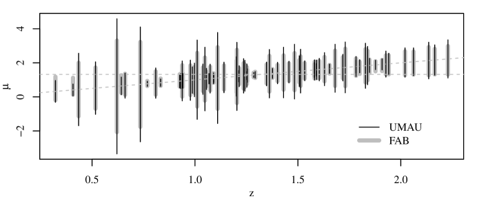
Figure 2: 95% FAB and UMAU intervals for the Minnesota radon data.

To illustrate the difference between FAB and standard $t$-intervals in a multigroup setting, we recreate the household radon example from Yu and Hoff (2018). The data considered include log radon levels of 916 households, each located in one of 82 counties (these are the counties with two or more households in the study). The data and code for this example are available via the R-package fabCI (Hoff and Yu, 2021). We model the sample mean in county $i$ as $Z_{i}\sim N(\mu_{i},\sigma^{2}_{i}/n_{i})$ where $\mu_{i}$ and $\sigma^{2}_{i}$ are unknown and $n_{i}$ is the sample size for county $i$. After fitting a normal random effects model that presumes $\mu_{1},\ldots,\mu_{n}\sim$ i.i.d.  $N(\phi,\tau^{2})$, it is ascertained that the across-group variance of the $\mu_{i}$’s is substantially smaller than the variability $\sigma^{2}_{i}/n_{i}$ of $Z_{i}$ for most groups, suggesting that across-group information sharing is likely to be beneficial. County-specific 95% FAB intervals are displayed in Figure 2, along with the direct $t$-intervals, which are the UMAU intervals for this normal sampling model. The FAB intervals are narrower than the UMAU intervals for 77 of the 82 counties, with UMAU intervals being 30% wider on average across counties. Both procedures have exact $95\%$ frequentist coverage for each group (assuming within-group normality of the data), regardless of what the true values of $\mu_{1},\ldots,\mu_{n}$ are. As discussed above, empirical Bayes posterior intervals lack this group-specific coverage guarantee.

5 Summary

Bayesian methods are often advertised as providing ‘‘a proper accounting of uncertainty.’’ Too often though, empirical Bayes data analyses ignore the uncertainty in the estimation of the prior distribution. Ignatiadis and Wager highlight this issue and provide useful confidence interval procedures for assessing this uncertainty. As with many empirical Bayes procedures, those of IW focus on across-group inference. If interest is instead on group-specific inference, methods with different coverage properties may be desired.

References

- Hoff and Yu (2021) Hoff, P. and C. Yu (2021). fabCI: FAB Confidence Intervals. R package version 0.2.
- Ignatiadis and Wager (2021) Ignatiadis, N. and S. Wager (2021). Confidence intervals for nonparametric empirical bayes analysis. Journal of the American Statistical Association.
- Laird and Louis (1987) Laird, N. M. and T. A. Louis (1987). Empirical Bayes confidence intervals based on bootstrap samples. J. Amer. Statist. Assoc. 82(399), 739--757. With discussion and with a reply by the authors.
- Morris (1983) Morris, C. N. (1983). Parametric empirical Bayes confidence intervals. In Scientific inference, data analysis, and robustness (Madison, Wis., 1981), Volume 48 of Publ. Math. Res. Center Univ. Wisconsin, pp. 25--50. Academic Press, Orlando, FL.
- Pratt (1963) Pratt, J. W. (1963). Shorter confidence intervals for the mean of a normal distribution with known variance. The Annals of Mathematical Statistics 34(2), 574--586.
- Yu and Hoff (2018) Yu, C. and P. D. Hoff (2018). Adaptive multigroup confidence intervals with constant coverage. Biometrika 105(2), 319--335.