Resonance $X(4630)$

Abstract

We investigate the structure $X(4630)$ discovered by the LHCb collaboration in the process $B^{+}\rightarrow J/\psi\phi K^{+}$ as a resonance in the $J/\psi\phi$ mass distribution. We explore this resonance as a diquark-antidiquark state $X=[cs][\overline{c}\overline{s}]$ with spin-parities $J^{\mathrm{PC}}=1^{-+}$. Its mass and current coupling are calculated using the QCD two-point sum rule method by taking into account vacuum condensates up to dimension $10$. We also study decays of this tetraquark to mesons $J/\psi\phi$, $\eta_{c}\eta^{(\prime)}$, and $\chi_{c1}\eta^{(\prime)}$, and compute partial widths of these channels. To this end, we employ the light-cone sum rule approach and technical methods of soft-meson approximation to extract strong coupling at relevant tetraquark-meson-meson vertices. Our predictions for the mass $m=(4632\pm 60)~{}\mathrm{MeV}$ and width $\Gamma=(159\pm 31)~{}\mathrm{MeV}$ of $X$ are in a very nice agreement with recent measurements of the LHCb collaboration. These results allow us to interpret the resonance $X(4630)$ as the tetraquark $X$ with spin-parities $J^{\mathrm{PC}}=1^{-+}$.

I Introduction

Recently the LHCb collaboration informed about new charmonium-like resonances $Z_{cs}$ and $X$  observed in the process $B^{+}\rightarrow J/\psi\phi K^{+}$ in $J/\psi K^{+}$ and $J/\psi\phi$ invariant mass distributions LHCb:2021uow . The new resonances $Z_{cs}(4000)^{+}$ and $Z_{cs}(4220)^{+}$ were discovered in the $J/\psi K^{+}$ channel, and are presumably exotic mesons with a quark content $c\overline{c}u\overline{s}$. States fixed in the $J/\psi\phi$ channel should be composed of $c\overline{c}s\overline{s}$ quarks provided they are four-quark structures. New resonances in this channel $X(4630)$ and $X(4685)$ enriched a list of vector, axial-vector and scalar states discovered by LHCb during the last few years Aaij:2016iza ; LHCb:2016nsl . The collaboration also updated parameters of states seen at early stages of investigations.

These experimental results generated a theoretical activity aimed to explain obtained information in the context of various approaches of high energy physics. Studies were concentrated mainly around the resonances $X(4630)$ and $Z_{cs}$, in which authors calculated masses and magnetic moments of these states, and explored their decay channels Liu:2021xje ; Ozdem:2021yvo ; Yang:2021sue ; Wang:2021ghk ; Turkan:2021ome . Some of new states were explained as threshold effects as well Ge:2021sdq .

The structure $X(4630)$ is a wide resonance with the mass

$$m_{\exp}=(4626\pm 16_{-110}^{+18})~{}\mathrm{MeV},$$ (1)

and width

$$\Gamma_{\exp}=(174\pm 27_{-73}^{+134})~{}\mathrm{MeV},$$ (2)

respectively. The LHCb determined also the spin-parity of $X(4630)$ and fixed them $J^{\mathrm{P}}=1^{-}$.

It should be noted that, a vector structure $Y(4626)$ with the mass $4625.9_{-6.0}^{+6.2}(\mathrm{stat.})\pm 0.4(\mathrm{sys.})~{}\mathrm{MeV}$ and the width $49.8_{-11.5}^{+13.9}(\mathrm{stat.})\pm 4.0(\mathrm{sys.})~{}\mathrm{MeV}$ was seen by the Belle collaboration recently in the process $e^{+}e^{-}\rightarrow D_{s}^{\ast}D_{s1}(2536)$ Belle:2019qoi . This resonance can be considered as a member of $Y$ family of vector states discovered in electron-positron annihilations. Other members of this group are resonances $Y(4630)$ and $Y(4660)$. First of them was detected by Belle in the process $e^{+}e^{-}\rightarrow\Lambda_{c}^{+}\Lambda_{c}^{-}$ as a peak in the $\Lambda_{c}^{+}\Lambda_{c}^{-}$ invariant mass distribution Pakhlova:2008vn . Its parameters $m=4634_{-7}^{+8}(\mathrm{stat.})_{-8}^{+5}(\mathrm{sys.})~{}\mathrm{MeV}$ and $\Gamma=92_{-24}^{+40}(\mathrm{stat.})_{-21}^{+10}(\mathrm{sys.})~{}\mathrm{MeV}$ are close to ones of the resonance $Y(4626)$, and whether they are different states or not is under investigation. It is interesting that $Y(4630)$ was usually identified with the vector state $Y(4660)$ Dai:2017fwx .

The resonance $Y(4660)$, as a particle produced in $e^{+}e^{-}$ annihilation, bears the quantum numbers $J^{\mathrm{PC}}=1^{--}$. It was modeled as excited $5{}^{3}S_{1}$ and $6{}^{3}S_{1}$ charmonia, as a compound of the scalar $f_{0}(980)$ and vector $\psi(2S)$ mesons, or as a baryonium state. In our work Sundu:2018toi , we explored $Y(4660)$ by treating it as the diquark-antidiquark vector state $[cs][\overline{c}\overline{s}]$. We calculated the mass and current coupling of the tetraquark $[cs][\overline{c}\overline{s}]$, and also evaluated its full width. Our results for the mass and full width of the state $[cs][\overline{c}\overline{s}]$ allowed us to interpret it as the observed resonance $Y(4660)$.

From analysis of the decay channel $X(4630)\rightarrow J/\psi\phi$, it is clear, that $X(4630)$ is charmonium-like state probably with hidden strange component $s\overline{s}$. Then, in the four-quark model its quark content  should be $c\overline{c}s\overline{s}$. It is also evident that $C$-parity conservation implies that $X(4630)$ is $C$ parity positive particle, i.e., the quantum numbers of this resonance should be $J^{\mathrm{PC}}=1^{-+}$. In other words, it can be considered as $C=+1$ counterpart of the resonance $Y(4626)$. Spin-parities $J^{\mathrm{PC}}=1^{-+}$ exclude interpretation of $X(4630)$ as an ordinary meson, because these quantum numbers are not accessible in the conventional quark-antiquark model. In other words, the resonance $X(4630)$ may be a double-exotic state: It is composed of four quarks and carries exotic quantum numbers.

Four valence quarks can be grouped in different ways to form a single structure. Indeed, they may form two conventional colorless mesons and constitute a hadronic molecule. Alternatively, four quarks $c\overline{c}s\overline{s}$ may build a diquark-antidiquark state $[cs][\overline{c}\overline{s}]$. The resonance $X(4630)$ was examined in the context of both these models. Thus, it was considered in Ref. Yang:2021sue as the molecule $D_{s}^{\ast}\overline{D}_{s1}(2536)$ with required spin-parities.  An analysis was performed there using the one-boson-exchange method. The mass of the molecule $D_{s}^{\ast}\overline{D}_{s1}$ was found equal to $4644~{}\mathrm{MeV}$ which is consistent with the LHCb data. The authors also emphasized, that a decay to a meson pair $J/\psi\phi$ is the main decay channel of the molecule $D_{s}^{\ast}\overline{D}_{s1}$.

The molecule model for $Y(4626)$ was used in Ref. He:2019csk , in which it was examined as a system $J^{\mathrm{PC}}=1^{--}$ appearing from the interaction $D_{s}^{\ast}\overline{D}_{s1}-D_{s}\overline{D}_{s1}$. In this article structures with spin-parities $J^{\mathrm{PC}}=0^{--},\ 0^{-+},\ 1^{-+}$ and others were explored as well. This treatment for the masses of the molecules $D_{s}^{\ast}\overline{D}_{s1}$ with $J^{\mathrm{PC}}=1^{--}$ and $J^{\mathrm{PC}}=1^{-+}$ leads to predictions $4646~{}\mathrm{MeV}$ and $4648~{}\mathrm{MeV}$, respectively. Heavy-antiheavy hadronic molecules built of the $S$-wave charmed mesons and baryons were studied also in Ref. Dong:2021juy . The authors assumed that interaction between mesons (baryons) is saturated by a meson exchange, and searched for poles in such systems by solving the Bethe-Salpeter equation.

In the framework of the QCD sum rule method a diquark-antidiquark option was considered in Ref. Wang:2013exa . The result of this article for the mass of the tetraquark $[cs][\overline{c}\overline{s}]$ with $J^{\mathrm{PC}}=1^{-+}$ equals to $4.63_{-0.08}^{+0.11}~{}\mathrm{GeV}$ and agrees with the new LHCb data. As is seen, almost all models for $X(4630)$ and predictions for its mass extracted using various methods within errors are consistent with experimental data. Stated differently, masses of exotic states do not provide information sufficient to verify different models by confronting them with each another or/and experimental data. Therefore, besides computations of the mass, there is a necessity to evaluate the full width of $X(4630)$ as precise as possible.

In the present work, we are going to fulfill this program and calculate the mass and width of the resonance $X(4630)$. We treat $X(4630)$ as diquark-antidiquark vector state $X=[cs][\overline{c}\overline{s}]$ with spin-parities $J^{\mathrm{PC}}=1^{-+}$. Investigations are performed in the context of the QCD sum rule method Shifman:1978bx ; Shifman:1978by , which is one of powerful nonperturbative tools of high energy physics. It allows one to compute parameters not only of conventional mesons and baryons, but also of multiquark hadrons Agaev:2020zad ; Albuquerque:2018jkn .

The mass and current coupling of the tetraquark $X$ are calculated in the framework of the QCD two-point sum rule approach. In these calculations, we take into account various quark, gluon, and mixed vacuum condensates up to dimension $10$. To investigate numerous decay channels of $X$, we use the light-cone sum rule (LCSR) method Balitsky:1989ry . Most of tetraquarks are strong-interaction unstable particles and decay into two conventional mesons. The resonance $X(4630)$ decays primarily to a pair of mesons $J/\psi\phi$ which is experimentally confirmed fact. In the present work, we study decays of the tetraquark $X$ not only to $J/\psi\phi$, but also to $\eta_{c}\eta^{(\prime)}$, and $\chi_{c1}\eta^{(\prime)}$ mesons saturating by these five channels its full width. The process $X\rightarrow J/\psi\phi$ is the dominant decay channel of the tetraquark $X$, whereas remaining modes are subdominant ones, but their contributions are important to evaluate the full width of $X$.

Partial widths of aforementioned decays are determined by strong couplings at relevant vertices. For instance, in the case of the dominant decay this is a strong coupling $G$ at the vertex $XJ/\psi\phi$. Calculation of the strong coupling at the tetraquark and two mesons vertex $XJ/\psi\phi$ in the LCSR method necessitates usage of complementary technical tools. A reason is that $X$ is built of four valence quarks, and the light-cone expansion of the relevant nonlocal correlator leads to expressions which instead of distribution amplitudes of the $\phi$ meson depend on its local matrix elements. To preserve the four-momentum at the vertex $XJ/\psi\phi$, in this situation one needs to impose additional kinematical restriction on the momentum of the $\phi$ meson. Troubles encountered afterward can be handled by including into analysis technical methods known as a soft-meson approximation Ioffe:1983ju ; Braun:1995 . The soft-meson approximation was adapted for investigation of tetraquarks in Ref. Agaev:2016dev , and applied to explore decays some of such particles (see, for example, Ref. Agaev:2020zad ). In present article, strong couplings at relevant vertices are computed by including into analysis nonperturbative terms up to dimension $8$. The coupling $G$ receives a contribution also from twist $4$ matrix element of the $\phi$ meson.

This article is organized in the following way: The mass and current coupling of the tetraquark $X$ are computed in Section II. We calculate the strong coupling $G$ of particles at the vertex $XJ/\psi\phi$ in Section III. Here, we find also the partial width of the decay $X\rightarrow J/\psi\phi$. Section IV is devoted to analysis of the processes $X\rightarrow\eta_{c}\eta^{(\prime)}$ and $X\rightarrow\chi_{c1}\eta^{(\prime)}$, and to computation of their partial widths. To this end, we calculate couplings $g_{1}$ and $g_{2}$ corresponding to vertices $X\eta_{c}\eta$ and $X\eta_{c}\eta^{\prime}$, respectively. Strong couplings $g_{3}$ and $g_{4}$ required to study decays $X\rightarrow\chi_{c1}\eta^{(\prime)}$ are found also in this section. In Sec. V, we confront our results with LHCb data for the resonance $X(4630)$. This section contains also our concluding remarks.

II Mass and current coupling of the tetraquark $X$

Sum rules to calculate the mass $m$ and current coupling $f$  of the tetraquark $X$ can be derived from analysis of the correlation function

$$\Pi_{\mu\nu}(p)=i\int d^{4}xe^{ipx}\langle 0|\mathcal{T}\{J_{\mu}(x)J_{\nu}^{{\dagger}}(0)\}|0\rangle,$$ (3)

where $J_{\mu}(x)$ is the interpolating current for the $X$ state, and $\mathcal{T}$ is time-ordered product of two currents.

The current with required properties has the following form

$$J_{\mu}(x) = \epsilon\widetilde{\epsilon}\left[s_{b}^{T}(x)C\gamma_{5}c_{c}(x)\overline{s}_{d}(x)\gamma_{5}\gamma_{\mu}C\overline{c}_{e}^{T}(x)\right.$$ (4)

$$\left.-s_{b}^{T}(x)C\gamma_{\mu}\gamma_{5}c_{c}(x)\overline{s}_{d}(x)\gamma_{5}C\overline{c}_{e}^{T}(x)\right],$$

where $\epsilon\widetilde{\epsilon}=\epsilon_{abc}\epsilon_{ade}$, and $a$, $b$, $c$, $d$, and $e$ are color indices. In expression above $C$ is the charge conjugation matrix.

The current $J_{\mu}(x)$ describes the tetraquark composed of the color antitriplet scalar diquark $\epsilon s^{T}C\gamma_{5}c$ (vector diquark $\epsilon s^{T}C\gamma_{\mu}\gamma_{5}c$) and color triplet vector antidiquark $\widetilde{\epsilon}\overline{s}\gamma_{5}\gamma_{\mu}C\overline{c}^{T}$ (scalar antidiquark $\widetilde{\epsilon}\overline{s}\gamma_{5}C\overline{c}^{T}$). This current belongs to antitriplet-triplet representation $\mathbf{[}\overline{\mathbf{3}_{\mathbf{c}}}\mathbf{]}_{cs}\otimes\mathbf{[3}_{\mathbf{c}}\mathbf{]}_{\overline{c}\overline{s}}$ of the color group $SU_{c}(3)$. Because the scalar diquark configuration is most attractive and stable two-quark system Jaffe:2004ph , the current $J_{\mu}(x)$ corresponds to a ground-state vector particle with lowest mass and required spin-parities.

To derive desired sum rules, we write down the correlation function $\Pi_{\mu\nu}(q)$ using the mass and current coupling of the state $X$. For these purposes, we insert into the correlation function a complete set of states with quantum numbers of $X$ and carry out in Eq. (3) integration over $x$. As a result, we get

$$\Pi_{\mu\nu}^{\mathrm{Phys}}(p)=\frac{\langle 0|J_{\mu}|X(p,\varepsilon\rangle\langle X(p,\varepsilon)|J_{\nu}^{\dagger}|0\rangle}{m^{2}-p^{2}}+\cdots,$$ (5)

with $m$ being the mass of $X$. In Eq. (5) dots stand for contributions of higher resonances and continuum states. We introduce the current coupling $f$ by means of the matrix element

$$\langle 0|J_{\mu}|X(p,\varepsilon)\rangle=fm\varepsilon_{\mu},$$ (6)

where $\varepsilon_{\mu}$ is the polarization vector of the tetraquark $X$. In terms of $m$ and $f$, the correlation function can be rewritten in the following form

$$\Pi_{\mu\nu}^{\mathrm{Phys}}(p)=\frac{m^{2}f^{2}}{m^{2}-p^{2}}\left(-g_{\mu\nu}+\frac{p_{\mu}p_{\nu}}{m^{2}}\right)+\cdots.$$ (7)

We calculate the QCD side of the correlation function $\Pi_{\mu\nu}(p)$ using explicit expression of the current $J_{\mu}(x)$ and obtain $\Pi_{\mu\nu}^{\mathrm{OPE}}(p)$ in terms of heavy and light quark propagators. Then for $\Pi_{\mu\nu}^{\mathrm{OPE}}(p)$, we get the following formula

$$\Pi_{\mu\nu}^{\mathrm{OPE}}(p)=i\int d^{4}xe^{ipx}\epsilon\widetilde{\epsilon}\epsilon^{\prime}\widetilde{\epsilon}^{\prime}\left\{\mathrm{Tr}\left[\gamma_{5}\widetilde{S}_{s}^{bb^{\prime}}(x)\gamma_{5}\right.\right.$$

$$\left.\times S_{c}^{cc^{\prime}}(x)\right]\mathrm{Tr}\left[\gamma_{5}\gamma_{\mu}\widetilde{S}_{c}^{ee^{\prime}}(-x)\gamma_{\nu}\gamma_{5}S_{s}^{dd^{\prime}}(-x)\right]$$

$$-\mathrm{Tr}\left[\gamma_{5}\gamma_{\mu}\widetilde{S}_{c}^{e^{\prime}e}(-x)\gamma_{5}S_{s}^{d^{\prime}d}(-x)\right]\mathrm{Tr}\left[\gamma_{5}\gamma_{\nu}\widetilde{S}_{s}^{bb^{\prime}}(x)\right.$$

$$\times\left.\gamma_{5}S_{c}^{cc^{\prime}}(x)\right]-\mathrm{Tr}\left[\gamma_{5}\widetilde{S}_{c}^{e^{\prime}e}(-x)\gamma_{\nu}\gamma_{5}S_{s}^{d^{\prime}d}(-x)\right]$$

$$\times\mathrm{Tr}\left[\gamma_{5}\widetilde{S}_{s}^{bb^{\prime}}(x)\gamma_{\mu}\gamma_{5}S_{c}^{cc^{\prime}}(x)\right]+\mathrm{Tr}\left[\gamma_{5}\gamma_{\nu}\widetilde{S}_{s}^{bb^{\prime}}(x)\right.$$

$$\left.\left.\times\gamma_{\mu}\gamma_{5}S_{c}^{cc^{\prime}}(x)\right]\mathrm{Tr}\left[\gamma_{5}\widetilde{S}_{c}^{e^{\prime}e}(-x)\gamma_{5}S_{s}^{dd^{\prime}}(-x)\right]\right\},$$ (8)

where $\epsilon^{\prime}\widetilde{\epsilon}^{\prime}=\epsilon_{a^{\prime}b^{\prime}c^{\prime}}\epsilon_{a^{\prime}d^{\prime}e^{\prime}}$. In Eq. (8) $S_{s}^{ab}(x)$ and $S_{c}^{ab}(x)$ are the $s$ and $c$-quark propagators, respectively. Their explicit expressions are collected in Appendix. Here, we also use the notation

$$\widetilde{S}_{s(c)}(x)=CS_{s(c)}^{T}(x)C.$$ (9)

To continue our analysis, we have to choose same structures both in $\Pi_{\mu\nu}^{\mathrm{Phys}}(p)$ and $\Pi_{\mu\nu}^{\mathrm{OPE}}(p)$. For our purposes, it is convenient to work with terms proportional to $-g_{\mu\nu}$, i. e., with invariant amplitude $\Pi^{\mathrm{Phys}}(p^{2})=m^{2}f^{2}/(m^{2}-p^{2})+\cdots$. This function receives contributions only from spin-$1$ particles and are free of contaminations. The amplitude $\Pi^{\mathrm{Phys}}(p^{2})$ can be expressed by the dispersion integral

$$\Pi^{\mathrm{Phys}}(p^{2})=\int_{4\mathcal{M}^{2}}^{\infty}\frac{\rho^{\mathrm{Phys}}(s)ds}{s-p^{2}}+\cdots,$$ (10)

where $\mathcal{M=}m_{c}+m_{s}$, and dots indicate subtraction terms necessary to make the whole expression finite. The imaginary part of the amplitude $\Pi^{\mathrm{Phys}}(p^{2})$ constitutes the spectral density $\rho^{\mathrm{Phys}}(s)$, which can be written down in the following form

$$\rho^{\mathrm{Phys}}(s)=\frac{1}{\pi}\mathrm{Im}\Pi^{\mathrm{Phys}}(s)=m^{2}f^{2}\delta(s-m^{2})+\rho^{\mathrm{h}}(s).$$ (11)

Here, contribution of the ground-state particle (the pole term) is separated from one due to higher resonances and continuum states: the latter is characterized by an unknown hadronic spectral density $\rho^{\mathrm{h}}(s)$. It is not difficult to see that $\rho^{\mathrm{Phys}}(s)$ substituted into Eq. (10) leads to the expression of the ground-state term

$$\Pi^{\mathrm{Phys}}(p^{2})=\frac{m^{2}f^{2}}{m^{2}-p^{2}}+\int_{4\mathcal{M}^{2}}^{\infty}\frac{\rho^{\mathrm{h}}(s)ds}{s-p^{2}}.$$ (12)

The obtained formula contains also a contribution coming from higher resonances and continuum states.

The amplitude $\Pi^{\mathrm{OPE}}(p^{2})$ can be calculated theoretically in deep Euclidean region $p^{2}\ll 0$ in the operator product expansion ($\mathrm{OPE}$) with certain accuracy. The coefficient functions in this expansion could be found using methods of perturbative QCD (PQCD), whereas nonperturbative information is encoded by vacuum expectation values of various quark, gluon and mixed operators. Having continued $\Pi^{\mathrm{OPE}}(p^{2})$ analytically to the Minkowski domain and computed its imaginary part one determines the two-point spectral density $\rho^{\mathrm{OPE}}(s)$. In the region $p^{2}\ll 0$ one applies also the Borel transformation to remove subtraction terms in the dispersion integral and suppress contributions of higher resonances and continuum states. In the case of $\Pi^{\mathrm{Phys}}(p^{2})$, we find

$$\mathcal{B}\Pi^{\mathrm{Phys}}(p^{2})=m^{2}f^{2}e^{-m^{2}/M^{2}}+\int_{4\mathcal{M}^{2}}^{\infty}ds\rho^{\mathrm{h}}(s)e^{-s/M^{2}},$$ (13)

with $M^{2}$ being the Borel parameter. Similar dispersion representation can be written down for $\Pi^{\mathrm{OPE}}(p^{2})$ in terms of $\rho^{\mathrm{OPE}}(s)$ as well. Later, using assumption about hadron-parton duality and matching $\rho^{\mathrm{h}}(s)\simeq\rho^{\mathrm{OPE}}(s)$ in duality region, it is possible to subtract second term in Eq. (13) from the QCD side of the sum rule and get

$$m^{2}f^{2}e^{-m^{2}/M^{2}}=\int_{4\mathcal{M}^{2}}^{s_{0}}ds\rho^{\mathrm{OPE}}(s)e^{-s/M^{2}}+\Pi(M^{2}),$$ (14)

where $s_{0}$ is continuum subtraction parameter. The second component of the invariant amplitude $\Pi(M^{2})$ contains nonperturbative contributions computed directly from $\Pi_{\mu\nu}^{\mathrm{OPE}}(p)$.

As is seen, physical parameters $m$ and $f$ of the tetraquark are expressed in terms of $\rho^{\mathrm{OPE}}(s)$ and $\Pi(M^{2})$ calculated in quark-gluon degrees of freedom. To complete a system of equations and determine the mass and coupling of the tetraquark $X$, we act by the operator $d/d(-1/M^{2})$ to both sides of the equality Eq. (14), and, by this way, find missed second expression. This system can be solved, and sum rules for the mass $m$ and coupling $f$ read

$$m^{2}=\frac{\Pi^{\prime}(M^{2},s_{0})}{\Pi(M^{2},s_{0})},$$ (15)

and

$$f^{2}=\frac{e^{m^{2}/M^{2}}}{m^{2}}\Pi(M^{2},s_{0}).$$ (16)

Here, we denote r.h.s. of Eq. (14) as $\Pi(M^{2},s_{0})$, and introduce also a function $\Pi^{\prime}(M^{2},s_{0})=d\Pi(M^{2},s_{0})/d(-1/M^{2})$.

In the present article, $\Pi(M^{2},s_{0})$ is calculated at the leading order of PQCD by taking into account quark, gluon and mixed vacuum condensates up to dimension $10$. Details of computations of the spectral density $\rho^{\mathrm{OPE}}(s)$ and function $\Pi(M^{2})$ can be found, for instance, in Ref. Agaev:2016dev . Therefore, we do not consider here these usual operations, and move explicit expression of the function $\Pi(M^{2},s_{0})$ to Appendix.

The sum rules for the mass and coupling given by Eqs. (15) and (16) contain quark, gluon and mixed condensates which are universal parameters of computations. They depend also masses of $c$ and $s$ quarks. Numerical values all of these parameters are listed below

$$\langle\overline{q}q\rangle=-(0.24\pm 0.01)^{3}~{}\mathrm{GeV}^{3},\ \langle\overline{s}s\rangle=(0.8\pm 0.1)\langle\overline{q}q\rangle,$$

$$\langle\overline{s}g_{s}\sigma Gs\rangle=m_{0}^{2}\langle\overline{s}s\rangle,\ m_{0}^{2}=(0.8\pm 0.1)~{}\mathrm{GeV}^{2},\$$

$$\langle\frac{\alpha_{s}G^{2}}{\pi}\rangle=(0.012\pm 0.004)~{}\mathrm{GeV}^{4},$$

$$\langle g_{s}^{3}G^{3}\rangle=(0.57\pm 0.29)~{}\mathrm{GeV}^{6},$$

$$m_{c}=(1.275\pm 0.025)~{}\mathrm{GeV}.\ \ \ m_{s}=93_{-5}^{+11}~{}\mathrm{MeV}.\text{ }$$ (17)

The sum rules are functions also of auxiliary parameters $M^{2}$ and $s_{0}$, which have to obey standard constraints imposed on them by the sum rule method. This means, that in the working regions of the parameters $M^{2}$ and $s_{0}$ a pole contribution ($\mathrm{PC}$) should dominate in the sum rules and the operator product expansion should converge rapidly. To quantify these constraints and use them to fix working windows for $M^{2}$ and $s_{0}$, we introduce expressions

$$\mathrm{PC}=\frac{\Pi(M^{2},s_{0})}{\Pi(M^{2},\infty)}.$$ (18)

and

$$R(M^{2})=\frac{\Pi^{\mathrm{DimN}}(M^{2},s_{0})}{\Pi(M^{2},s_{0})},$$ (19)

where $\Pi^{\mathrm{DimN}}(M^{2},s_{0})$ is a contribution of the last three terms in $\mathrm{OPE}$, i.e., $\mathrm{DimN=Dim(8+9+10)}$.

The formula Eq. (18) determines a contribution of the pole term to the function $\Pi(M^{2},s_{0})$. In our present study, we adopt the limit $\mathrm{PC\geqslant 0.2}$, which is typical for multiquark particles. The convergence of the operator product expansion is examined by means of the expression Eq. (19): The convergence of $\mathrm{OPE}$ is fulfilled if at the minimum of the Borel parameter the ratio $R(M^{2})$ does not exceed $0.01$. The mass and current coupling of $X$ obtained by means of the sum rules, in general, have not to depend on the Borel parameter, but in actual computations, one can only limit its influence on obtained predictions. Thus, a stability of extracted results is among employed constraints to get the parameters $M^{2}$ and $s_{0}$.

Computations show that the working regions that meet all these constraints are

$$M^{2}\in[5.5,6.5]~{}\mathrm{GeV}^{2},\ s_{0}\in[24,25]~{}\mathrm{GeV}^{2}.$$ (20)

In fact, in these regions the pole contribution varies within a range $0.66\leq\mathrm{PC}\leq 0.26$. The convergence of $\mathrm{OPE}$ is also satisfied, because at $M^{2}=5.5~{}\mathrm{GeV}^{2}$, we fix $R(M^{2})\leq 0.01$.

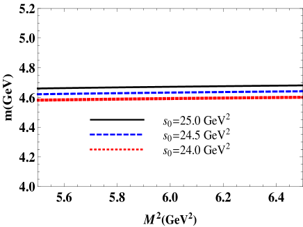
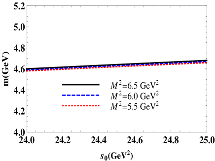
Figure 1: The mass of the tetraquark $X(4630)$ as a function of the Borel parameter $M^{2}$ at fixed $s_{0}$ (left panel), and as a function of the continuum threshold $s_{0}$ at fixed $M^{2}$ (right panel).

To extract numerical values of the mass $m$ and coupling $f$, we calculate them at different choices of the parameters $M^{2}$ and $s_{0}$, and find their mean values averaged over the working regions Eq. (20). For $m$ and $f$ these calculations yield

$$m = (4632\pm 60)~{}\mathrm{MeV},$$

$$f = (9.2\pm 0.8)\times 10^{-3}~{}\mathrm{GeV}^{4}.$$ (21)

The values from Eq. (21) correspond to sum rules’ results computed at middle point of the working regions, i.e., to results at the points $M^{2}=6~{}\mathrm{GeV}^{2}$ and $s_{0}=24.5~{}\mathrm{GeV}^{2}$. At this point the pole contribution is $\mathrm{PC}\approx 0.51$, which guarantees reliability of obtained predictions, and a ground-state nature of $X$.

In Fig. 1, we plot the mass of the tetraquark $X$ as functions of the parameters $M^{2}$ and $s_{0}$. As is seen, the mass $m$ is sensitive to a choice of $M^{2}$ and $s_{0}$. It is also evident that within limits $M^{2}\in[5.5,6.5]~{}\mathrm{GeV}^{2}$ this dependence is weak and theoretical errors do not exceed $1.5\%$, whereas similar estimate for the coupling gives $9\%$. This effect has simple explanation: The mass of the tetraquark is determined by the ratio of the correlation functions Eq. (15). As a result, this ratio smooths dependence of $m$ on the parameter $M^{2}$, which is not a case for the coupling Eq. (16).

The mass of the tetraquark $X$ obtained in the present work is in excellent agreement with the LHCb data for the mass of the resonance $X(4630)$. At this phase of our studies, we can conclude that $X(4630)$ is the diquark-antidiquark state $X=[cs][\overline{c}\overline{s}]$ with spin-parities $J^{\mathrm{PC}}=1^{-+}$.

III Decay $X\rightarrow J/\psi\phi$  

The resonance $X(4630)$ was observed in the invariant mass distribution of the $J/\psi\phi$ mesons. Hence, the process $X(4630)\rightarrow J/\psi\phi$ can be considered as its dominant decay channel. In this section, we consider this decay and calculate partial width of the process $X\rightarrow J/\psi\phi$, which is governed by the strong coupling $G$ at the vertex $XJ/\psi\phi$.

In the context of the LCSR method the vertex $XJ/\psi\phi$ can be explored by means of the correlator

$$\Pi_{\mu\nu}(p,q)=i\int d^{4}xe^{ipx}\langle\phi(q)|\mathcal{T}\{J_{\mu}^{J/\psi}(x)J_{\nu}^{{\dagger}}(0)\}|0\rangle,$$ (22)

with $J_{\nu}$ and $J_{\mu}^{J/\psi}$ being the interpolating currents of the tetraquark $X$ and vector meson $J/\psi$, respectively. The $J_{\nu}$ is given by Eq. (4), and current $J_{\mu}^{J/\psi}$ has the form

$$J_{\mu}^{J/\psi}(x)=\overline{c}_{l}(x)\gamma_{\mu}c_{l}(x),$$ (23)

where $l=1,2,3$ is color index. In Eq. (22) $p$ and $q$ are the momenta of the $J/\psi$ and $\phi$ mesons. Then the 4-momentum of the the tetraquark $X$ is equal to $p^{\prime}=p+q$.

For on mass-shell $\phi$ meson $q^{2}=m_{\phi}^{2}$, the correlator $\Pi_{\mu\nu}(p,q)$ is a function of two independent variables $p^{2}$ and $p^{\prime 2}=(p+q)^{2}$. It can be expanded over  a set of Lorentz structures in terms of invariant amplitudes $\Pi_{i}(p^{2},p^{\prime 2})$ and mass factors $C_{i}(\{m^{2}\})$.  For our purposes, it is convenient to expand $\Pi_{\mu\nu}(p,q)$ in the following basis

$$\Pi_{\mu\nu}(p,q)=\Pi_{1}(p^{2},p^{\prime 2})C_{1}(\{m^{2}\})\varepsilon_{\mu}^{\ast}(q)p_{\nu}$$

$$+\Pi_{2}(p^{2},p^{\prime 2})C_{2}(\{m^{2}\})\varepsilon_{\nu}^{\ast}(q)p_{\mu}++\Pi_{3}(p^{2},p^{\prime 2})$$

$$\times C_{3}(\{m^{2}\})\varepsilon^{\ast}(q)\cdot pp_{\mu}p_{\nu}+\Pi_{4}(p^{2},p^{\prime 2})$$

$$\times C_{4}(\{m^{2}\})\varepsilon^{\ast}(q)\cdot pg_{\mu\nu}+\cdots,$$ (24)

where $\varepsilon^{\ast}(q)$ is polarization vector of the $\phi$ meson. The factors $C_{i}(\{m^{2}\})$ depend on some combination of particles’ masses $\{m^{2}\}=\{m^{2},m_{1}^{2},m_{\phi}^{2}\}$ , with $m_{1}$ and $m_{\phi}$ being masses of the $J/\psi$ and $\phi$ mesons, respectively.

The phenomenological side of the sum rule can be obtained from Eq. (22) by expressing $\Pi_{\mu\nu}(p,q)$ in terms of physical parameters of particles involved into the decay process. To explain this procedure, as an example, let us consider the amplitude $\Pi_{1}(p^{2},p^{\prime 2})$. Using the double dispersion relation Braun:1995 ; Colangelo:1997rp , for $\Pi_{1}(p^{2},p^{\prime 2})$ we get

$$\Pi_{1}(p^{2},p^{\prime 2})=\int\int\frac{\rho_{1}^{\mathrm{h}}(s_{1},s_{2})ds_{1}ds_{2}}{(s_{1}-p^{\prime 2})(s_{2}-p^{2})}$$

$$+\int\frac{\rho_{11}^{\mathrm{h}}(s_{1})ds_{1}}{(s_{1}-p^{\prime 2})}+\int\frac{\rho_{21}^{\mathrm{h}}(s_{2})ds_{2}}{(s_{2}-p^{2})}.$$ (25)

As is seen, Eq. (25) contains also single dispersion integrals which are necessary to make finite the whole expression.

The amplitude $\Pi_{1}(p^{2},p^{\prime 2})$ receives contributions from two channels: First channel contains vector tetraquarks $[cs][\overline{c}\overline{s}]$, whereas second one is a channel of vector charmonia. Separating in spectral density $\rho_{1}^{\mathrm{h}}(s_{1},s_{2})$ contributions of ground-state particles in these channels, i. e., contribution of the tetraquark $X$ and $J/\psi$ from effects of higher resonances and continuum states, we can model $\rho_{1}^{\mathrm{h}}(s_{1},s_{2})$ in the form Colangelo:1997rp

$$\rho_{1}^{\mathrm{h}}(s_{1},s_{2})=Gfmf_{1}m_{1}\delta(s_{1}-m^{2})\delta(s_{2}-m_{1}^{2})$$

$$+\rho_{1}^{\mathrm{h}}(s_{1},s_{2})\theta(s_{1}-s_{0})\theta(s_{2}-s_{0}^{\prime}),$$ (26)

where $G$ is the strong coupling, which should be extracted from relevant sum rule. The doubly spectral density $\rho_{1}^{\mathrm{h}}(s_{1},s_{2})$ contains also the current coupling $f$ of the tetraquark $X$ and decay constant $f_{1}$ of the $J/\psi$ meson, which are defined by Eq. (6) and by the matrix element

$$\langle 0|J_{\mu}^{J/\psi}|J/\psi\left(p\right)\rangle=f_{1}m_{1}\varepsilon_{\mu}(p),$$ (27)

respectively. Here, $\varepsilon_{\mu}(p)$ is the polarization vector of the $J/\psi$ meson.

Substituting $\rho_{1}^{\mathrm{h}}(s_{1},s_{2})$ into Eq. (25), we find

$$\Pi_{1}(p^{2},p^{\prime 2})=\frac{Gfmf_{1}m_{1}}{\left(p^{\prime 2}-m^{2}\right)\left(p^{2}-m_{1}^{2}\right)}C_{1}(\{m^{2}\})$$

$$+\underset{\sum}{\int\int}\frac{\rho_{1}^{\mathrm{h}}(s_{1},s_{2})ds_{1}ds_{2}}{(s_{1}-p^{\prime 2})(s_{2}-p^{2})}+\cdots,$$ (28)

where $\sum$ is a domain in the $(s_{1},s_{2})$ plane boundaries of which $(s_{0},\ s_{0}^{\prime})$ depend on parameters of a process under analysis. For the sake of brevity, we do not write down here single dispersion integrals and denote them by dots. The similar dispersion relations can be written down for remaining amplitudes, as well. Because the strong coupling $G$ is the same for all structures Bracco:2007sg , one gets

$$\Pi_{\mu\nu}^{\mathrm{Phys}}(p,q)=\frac{Gfmf_{1}m_{1}}{\left(p^{\prime 2}-m^{2}\right)\left(p^{2}-m_{1}^{2}\right)}$$

$$\times\left[C_{1}(\{m^{2}\})\varepsilon_{\mu}^{\ast}(q)p_{\nu}+C_{2}(\{m^{2}\})\varepsilon_{\nu}^{\ast}(q)p_{\mu}\right.$$

$${}+C_{3}(\{m^{2}\})\varepsilon^{\ast}(q)\cdot pp_{\mu}p_{\nu}+C_{4}(\{m^{2}\})$$

$$\left.\times\varepsilon^{\ast}(q)\cdot pg_{\mu\nu}+\cdots\right]+\Pi_{\mu\nu}^{(\mathrm{HR,C)}}(p,q).$$ (29)

Contributions stemming from higher resonances and continuum states are denoted in Eq. (29) by $\Pi_{\mu\nu}^{(\mathrm{HR,C)}}(p,q)$. We are interested in detailed analysis of the first term in $\Pi_{\mu\nu}^{\mathrm{Phys}}(p,q)$ Braun:1995 , with poles at $p^{2}$ and $p^{\prime 2}=(p+q)^{2}$.

The correlation function $\Pi_{\mu\nu}^{\mathrm{Phys}}(p,q)$ can be written down in the factorized form

$$\Pi_{\mu\nu}^{\mathrm{Phys}}(p,q)=\langle\phi(q)J/\psi\left(p\right)|X(p^{\prime})\rangle\frac{\langle X(p^{\prime})|J_{\nu}^{{\dagger}}|0\rangle}{\left(p^{\prime 2}-m^{2}\right)}$$

$$\times\frac{\langle 0|J_{\mu}^{J/\psi}|J/\psi\left(p\right)\rangle}{\left(p^{2}-m_{1}^{2}\right)}+\cdots,$$ (30)

where $mf$ and $m_{1}f_{1}$ are replaced by relevant martix elements (up to polararization vectors), whereas on-mass-shell matrix element $\langle\phi(q)J/\psi\left(p\right)|X(p^{\prime})\rangle$  defines the strong coupling $G\$at the vertex $XJ/\psi\phi$. It can be modeled in the following form

$$\langle\phi(q)J/\psi\left(p\right)|X(p^{\prime})\rangle=G\left[(q-p)_{\gamma}g_{\alpha\beta}-(p^{\prime}+q)_{\alpha}g_{\gamma\beta}\right.$$

$$\left.+(p^{\prime}+p)_{\beta}g_{\gamma\alpha}\right]\varepsilon^{\gamma}(p^{\prime})\varepsilon^{\ast\alpha}(p)\varepsilon^{\ast\beta}(q).$$ (31)

Then from Eq. (30) one can easily find that

$$\Pi_{\mu\nu}^{\mathrm{Phys}}(p,q)=\frac{Gfmf_{1}m_{1}}{\left(p^{\prime 2}-m^{2}\right)\left(p^{2}-m_{1}^{2}\right)}$$

$$\times\left[\frac{m_{1}^{2}-m^{2}-m_{\phi}^{2}}{m^{2}}\varepsilon_{\mu}^{\ast}(q)p_{\nu}+\frac{m^{2}-m_{1}^{2}-m_{\phi}^{2}}{m_{1}^{2}}\varepsilon_{\nu}^{\ast}(q)p_{\mu}\right.$$

$${}\left.-\frac{m^{2}+m_{1}^{2}-m_{\phi}^{2}}{m^{2}m_{1}^{2}}\varepsilon^{\ast}(q)\cdot pp_{\mu}p_{\nu}+2\varepsilon^{\ast}(q)\cdot pg_{\mu\nu}+\cdots\right]$$

$$+\Pi_{\mu\nu}^{(\mathrm{HR,C)}}(p,q),$$ (32)

where ellipses inside of the square brackets stand for terms that vanish in the limit $p^{\prime}\rightarrow p$ (see an explanation below). Comparing the correlation function $\Pi_{\mu\nu}^{\mathrm{Phys}}(p,q)$ in Eq. (32) with one from Eq. (29), one sees that they coincide with each other provided functions $C_{i}(\{m^{2}\})$ are given by formulas

$$C_{1}(\{m^{2}\}) = \frac{m_{1}^{2}-m^{2}-m_{\phi}^{2}}{m^{2}},$$

$$C_{2}(\{m^{2}\}) = \frac{m^{2}-m_{1}^{2}-m_{\phi}^{2}}{m_{1}^{2}},$$

$$C_{3}(\{m^{2}\}) = -\frac{m^{2}+m_{1}^{2}-m_{\phi}^{2}}{m^{2}m_{1}^{2}},$$

$$C_{4}(\{m^{2}\}) = 2.$$ (33)

There are a few Lorentz structures in Eq. (32), which may be employed to construct a sum rule equality. In the present work, we choose to work with the structure $\sim\varepsilon_{\mu}^{\ast}(q)p_{\nu}$ and denote relevant invariant amplitude by $\Pi^{\mathrm{Phys}}(p^{2},p^{\prime 2})$.

At the next phase of studies, we have to calculate the correlation function $\Pi_{\mu\nu}^{\mathrm{OPE}}(p,q)$ using quark-gluon degrees of freedom. To this end, we insert expressions of the currents $J_{\mu}^{J/\psi}(x)$ and $J_{\nu}^{{\dagger}}(0)$ into Eq. (22), contract relevant quark fields and replace them by corresponding quark propagators. In full LCSR treatment of vertices, for instance, composed of three conventional mesons, a final expression obtained for $\Pi_{\mu\nu}^{\mathrm{OPE}}(p,q)$ depends on propagators and distribution amplitudes (DAs) of a meson. Afterwards, separating in the correlation function a chosen Lorentz structure and corresponding invariant amplitude $\Pi^{\mathrm{OPE}}(p^{2},(p+q)^{2})$, one should calculate it in the regions $s_{1}=(p+q)^{2}\ll 0$ and $s_{2}=p^{2}\ll 0$, where methods of PQCD are applicable. After analytical continuation of $\Pi^{\mathrm{OPE}}(s_{1},s_{2})$ to Minkowski domain, computation its imaginary part over variables $s_{1}$ and $s_{2}$, one can determine a spectral density $\rho^{\mathrm{OPE}}(s_{1},s_{2})$. Then using parton-hadron duality assumption $\rho^{\mathrm{h}}(s_{1},s_{2})\simeq\rho^{\mathrm{OPE}}(s_{1},s_{2})$ and performing double Borel transformations over variables $p^{2}\ll 0$ and $p^{\prime 2}\ll 0$ to suppress effects of higher resonances and remove single dispersion integrals, one finds a sum rule which expresses an on-mass-shell three-meson coupling in terms of $\rho^{\mathrm{OPE}}(s_{1},s_{2})$.

In the case under discussion, i. e., for tetraquark-meson-meson vertex $XJ/\psi\phi$ full LCSR scheme outlined above has to be modified. Reasons for that are connected with features of the function $\Pi_{\mu\nu}^{\mathrm{OPE}}(p,q)$. In fact, QCD expression for $\Pi_{\mu\nu}^{\mathrm{OPE}}(p,q)$ obtained using quark propagators is given by the formula

$$\Pi_{\mu\nu}^{\mathrm{OPE}}(p,q)=-i\int d^{4}xe^{ipx}\epsilon\widetilde{\epsilon}\left\{\left[\gamma_{5}\widetilde{S}_{c}^{lc}(x)\gamma_{\mu}\right.\right.$$

$$\left.\left.\times\widetilde{S}_{c}^{el}(-x)\gamma_{\nu}\gamma_{5}\right]+\left[\gamma_{\nu}\gamma_{5}\widetilde{S}_{c}^{lc}(x){}\gamma_{\mu}\widetilde{S}_{c}^{el}(-x){}\gamma_{5}\right]\right\}_{\alpha\beta}$$

$$\times\langle\phi(q)|\overline{s}_{\alpha}^{b}(0)s_{\beta}^{d}(0)|0\rangle,$$ (34)

where $\alpha$ and $\beta$ are spinor indices.

As is seen, the function $\Pi_{\mu\nu}^{\mathrm{OPE}}(p,q)$ instead of $\phi$ meson’s distribution amplitudes depends on its local matrix elements. The emerged situation has simple explanation: The meson $J/\psi$ is composed of $c$ quark and antiquark at $x$ which can be contracted only with $c$-antiquark and quark from the tetraquark $X$. As a result, remaining $s$-quark fields in the current $J_{\nu}^{{\dagger}}(0)$ located at the space-time position $x=0$ establish local matrix elements of the $\phi$ meson.

To understand consequences of this situation, it is convenient to perform following transformations

$$\overline{s}_{\alpha}^{b}s_{\beta}^{d}\rightarrow\frac{1}{12}\delta^{bd}\Gamma_{\beta\alpha}^{j}\left(\overline{s}\Gamma^{j}s\right),$$ (35)

where $\Gamma^{j}$ is the full set of Dirac matrices,

$$\Gamma^{j}=\mathbf{1,\ }\gamma_{5},\ \gamma_{\mu},\ i\gamma_{5}\gamma_{\mu},\ \sigma_{\mu\nu}/\sqrt{2}.$$ (36)

Let us note, that in Eq. (35), we use also the projector onto a color-singlet state $\delta^{bd}/3$.

After these manipulations, it is easy to carry out a color summation. Later, we substitute quark propagators into obtained expression and perform $4$-dimensional integration over $x$. This integration creates in the integrand the delta function $\delta^{4}(p^{\prime}-p)$, which as an argument contains only four-momenta of the tetraquark $X$ and meson $J/\psi$. Therefore, subsequent integration over $p$ or $p^{\prime}$  sets $p=p^{\prime}$, which is the consequence of the four-momentum conservation at the vertex $XJ/\psi\phi$. Stated differently, to preserve the four-momentum at the tetraquark-meson-meson vertex one has to choose $q=0$. In the full LCSR this is known as the soft-meson approximation Braun:1995 . At vertices of ordinary mesons $q\neq 0$, and only in the soft-meson limit, one equates $q$ to zero, whereas the tetraquark-meson-meson vertex can be explored in the framework of the LCSR method only for $q=0$. It is worth emphasizing that tetraquark-tetraquark-meson vertices can be explored using the full LCSR method: Correlation function of a such vertex depends on distribution amplitudes of a final meson Agaev:2016srl ; Sundu:2017xct ; Agaev:2019coa . For our purposes, it is important that both the soft-meson approximation and full LCSR treatment of the ordinary mesons’ vertices lead for the strong couplings to very close numerical predictions Braun:1995 , hence our treatment of the coupling $G$ should give a reliable result.

Equation (35) applied to $\Pi_{\mu\nu}^{\mathrm{OPE}}(p,0)$ generates different local matrix elements of the $\phi$ meson, which are known and can be used to find analytical expression and carry out numerical computations. Analysis confirms, that only two matrix elements of the $\phi$ meson contribute to the correlation function. First of them is twist-$2$ matrix element

$$\langle\phi(q)|\overline{s}(0)\gamma_{\mu}s(0)|0\rangle=f_{\phi}m_{\phi}\varepsilon_{\mu}^{\ast}(q),$$ (37)

where $f_{\phi}$ is the decay constant of $\phi$ meson. Second matrix element, which survives in the soft-meson limit, has twist $4$ and is given by the expression

$$\langle\phi(q)|\overline{s}(0)g\widetilde{G}_{\mu\nu}\gamma^{\nu}\gamma_{5}s(0)|0\rangle=f_{\phi}m_{\phi}^{3}\zeta_{4\phi}\varepsilon_{\mu}^{\ast}(q).$$ (38)

Here, $\widetilde{G}_{\mu\nu}=1/2\varepsilon_{\mu\nu\alpha\beta}G^{\alpha\beta}$ is the gluon dual field-strength tensor. The parameter $\zeta_{4\phi}=\pm 0.02$ was determined from the sum rule analysis in Ref. Ball:2007zt , and is small.

But before deriving the sum rule for the strong coupling $G$, the soft limit should be implemented also in the physical expression of the correlation function $\Pi_{\mu\nu}^{\mathrm{Phys}}(p,q)$. In the limit $q\rightarrow 0$, the ground-state term in $\Pi_{\mu\nu}^{\mathrm{Phys}}(p,0)$ can be modified with some accuracy in the following way

$$\frac{1}{\left(p^{\prime 2}-m^{2}\right)\left(p^{2}-m_{1}^{2}\right)}\rightarrow\frac{1}{\left(p^{2}-\widetilde{m}^{2}\right)^{2}},$$ (39)

where $\widetilde{m}^{2}$ is equal to $(m^{2}+m_{1}^{2})/2$. After this transformation instead of two single poles at $p^{\prime 2}=m^{2}$ and $p^{2}=m_{1}^{2}$, the function $\Pi^{\mathrm{Phys}}(p^{2},0)$ acquires one double-pole at $p^{2}=\widetilde{m}^{2}$.

Having fixed in $\Pi_{\mu\nu}^{\mathrm{OPE}}(p,0)$ an amplitude $\Pi^{\mathrm{OPE}}(p^{2})$ which corresponds to the structure $\sim\varepsilon_{\mu}^{\ast}(q)p_{\nu}$, and carried out calculations in the region $p^{2}\ll 0$ we find finally the spectral density $\rho^{\mathrm{OPE}}(s)$. But in the soft approximation the Borel transformation and subtraction procedure require more careful considerations than in full LCSR treatment. In the soft limit one performs Borel transformation over one variable $p^{2}\ll 0$, and in this case single dispersion integrals also contribute to hadronic part of the sum rules. These non-vanishing contributions correspond to transitions from the excited states in $X$ channel Braun:1995 . Therefore, before carrying out the continuum subtraction they should be excluded from $\mathcal{B}\Pi^{\mathrm{Phys}}(p^{2})$ by means of some prescription. This problem is solved by the operator Ioffe:1983ju ; Braun:1995

$$\mathcal{P}(M^{2},\widetilde{m}^{2})=\left(1-M^{2}\frac{d}{dM^{2}}\right)M^{2}e^{\widetilde{m}^{2}/M^{2}},$$ (40)

that acts to both sides of the sum rule. It eliminates unsuppressed terms in the physical side, but modifies also QCD side of the sum rule. Then contributions of higher resonances with regular behavior can be subtracted from the QCD side using the quark-hadron duality assumption.

The sum rule for the strong coupling $G$ reads

$$G=\frac{m}{fm_{1}f_{1}}\frac{\mathcal{P}(M^{2},\widetilde{m}^{2})\mathcal{B}\Pi^{\mathrm{OPE}}(p^{2})}{m_{1}^{2}-m^{2}-m_{\phi}^{2}}.$$ (41)

The Borel transformed and subtracted correlation function $\mathcal{B}\Pi^{\mathrm{OPE}}(p^{2})$ has the following form

$$\mathcal{B}\Pi^{\mathrm{OPE}}(p^{2})=\int_{4\mathcal{M}^{2}}^{s_{0}}ds\rho^{\mathrm{pert.}}(s)e^{-s/M^{2}}+\overline{\Pi}(M^{2}).$$ (42)

The integral in Eq. (42) is a perturbative term, where the spectral density $\rho^{\mathrm{pert.}}(s)$ is determined by the expression

$$\rho^{\mathrm{pert.}}(s)=\frac{f_{\phi}m_{\phi}m_{c}}{4\pi^{2}}\frac{\sqrt{s(s-4m_{c}^{2})}}{s}.$$ (43)

The second component of $\mathcal{B}\Pi^{\mathrm{OPE}}(p^{2})$, i.e., the function $\overline{\Pi}(M^{2})$ contains the twist-4 and nonperturbative contributions,

$$\overline{\Pi}(M^{2}) = \frac{f_{\phi}m_{\phi}^{3}m_{c}\zeta_{4\phi}}{16\pi^{2}}\int_{0}^{1}\frac{dx}{x(x-1)}e^{-m_{c}^{2}/M^{2}x(1-x)}$$ (44)

$$+\frac{f_{\phi}m_{\phi}m_{c}}{4}\mathcal{F}^{\mathrm{n.-pert.}}(M^{2}),$$

where $\mathcal{F}^{\mathrm{n.-pert.}}(M^{2})$ is given by the formula

$$\mathcal{F}^{\mathrm{n.-pert.}}(M^{2})=\Big{\langle}\frac{\alpha_{s}G^{2}}{\pi}\Big{\rangle}\int_{0}^{1}f_{1}(x,M^{2})dx-\Big{\langle}g_{s}^{3}G^{3}\Big{\rangle}$$

$$\times\int_{0}^{1}f_{2}(x,M^{2})dx-\Big{\langle}\frac{\alpha_{s}G^{2}}{\pi}\Big{\rangle}^{2}\int_{0}^{1}f_{3}(x,M^{2})dx.$$ (45)

The nonperturbative contributions of four, six and eight dimensions are proportional to $\langle\alpha_{s}G^{2}/\pi\rangle$, $\langle g_{s}^{3}G^{3}\rangle$ and $\langle\alpha_{s}G^{2}/\pi\rangle^{2}$, respectively. The functions $f_{i}(x,M^{2})$, $i=1,2,3$ are explicitly given below:

$$f_{1}(x,M^{2})=\frac{1}{18M^{4}x^{2}(1-x)^{2}}\left[8m_{c}^{2}(1-x)^{2}\right.$$

$$\left.+M^{2}(2-7x+9x^{2}-4x^{3}+2x^{4})\right]e^{-m_{c}^{2}/M^{2}x(1-x)},$$

(46)

$$f_{2}(x,M^{2})=\frac{1}{240M^{8}\pi^{2}x^{5}(x-1)^{5}}\left[2M^{4}x^{2}(1-x)^{2}\right.$$

$$\times\left(3-11x+15x^{2}-8x^{3}+4x^{4}\right)+24m_{c}^{4}(1-2x)^{2}$$

$$\times\left(-2-7x+17x^{2}-20x^{3}+10x^{4}\right)-3m_{c}^{2}M^{2}x$$

$$\times\left(4-49x+176x^{2}-293x^{3}+218x^{4}-26x^{5}\right.$$

$$\left.\left.-40x^{6}+10x^{7}\right)\right]e^{-m_{c}^{2}/M^{2}x(1-x)},$$ (47)

and

$$f_{3}(x,M^{2}) = \frac{16\pi^{2}m_{c}^{2}}{9M^{10}x^{3}(x-1)^{3}}\left(25m_{c}^{2}+6M^{2}x\right.$$ (48)

$$\left.-6M^{2}x^{2}\right)e^{-m_{c}^{2}/M^{2}x(1-x)}.$$

The width of the process $X\rightarrow J/\psi\phi$ is determined by the formula

$$\Gamma(X\rightarrow J/\psi\phi)=G^{2}\frac{\lambda(m,m_{1},m_{\phi})}{24\pi m^{2}}|M|^{2},$$ (49)

where

$$|M|^{2}=\frac{1}{4m^{2}m_{1}^{2}m_{\phi}^{2}}\left[m_{1}^{8}+8m_{1}^{6}(m^{2}+m_{\phi}^{2})\right.$$

$$+(m_{\phi}^{2}-m^{2})^{2}\left(m_{\phi}^{4}+10m_{\phi}^{2}m^{2}+m^{4}\right)$$

$$-2m_{1}^{4}\left(9m_{\phi}^{4}+16m_{\phi}^{2}m^{2}+9m^{4}\right)+8m_{1}^{2}$$

$$\left.\times\left(m_{\phi}^{6}-4m_{\phi}^{4}m^{2}-4m_{\phi}^{2}m^{4}+m^{6}\right)\right],$$ (50)

and $\lambda(a,b,c)$ is the function

$$\lambda(a,b,c)=\frac{\sqrt{a^{4}+b^{4}+c^{4}-2(a^{2}b^{2}+a^{2}c^{2}+b^{2}c^{2})}}{2a}.$$ (51)

Parameters	Values (in $\mathrm{MeV}$ units)
$m_{1}[m_{J/\psi}]$	$3096.900\pm 0.006$
$f_{1}[f_{J/\psi}]$	$409\pm 15$
$m_{2}[m_{\eta_{c}}]$	$2983.9\pm 0.5$
$f_{2}[f_{\eta_{c}}]$	$320\pm 40$
$m_{3}[m_{\chi_{1c}}]$	$3510.67\pm 0.05$
$f_{3}[f_{\chi_{1c}}]$	$344\pm 27$
$m_{\phi}$	$1019.461\pm 0.019$
$f_{\phi}$	$228.5\pm 3.6$
$m_{\eta}$	$547.862\pm 0.017$
$m_{\eta^{\prime}}$	$957.78\pm 0.06$

Table 1: Masses and decay constants of mesons, which have been used in numerical computations.

The sum rule Eq. (41) depends on the mass and decay constant of the $J/\psi$ and $\phi$ mesons: Their values are collected in Table 1. This table contains also spectroscopic parameters of other mesons which will be used in the next section. The masses of all mesons are borrowed from Ref. PDG:2020 . As the decay constants $f_{\phi}$ and $f_{1}$ of the vector mesons $\phi$ and $J/\psi$, we use their experimental values reported in Refs. Chakraborty:2017hry ; Kiselev:2001xa , respectively. For the decay constants $f_{2}$ and $f_{3}$ of the $\eta_{c}$ and $\chi_{1c}$ mesons, we utilize relevant sum rules’ predictions from Refs. Colangelo:1992cx and VeliVeliev:2012cc , respectively.

In numerical analysis, the parameters $M^{2}$ and $s_{0}$ are chosen as in Eq. (20). Computations allow us to find numerical value of the strong coupling $G$

$$G=0.85\pm 0.12.$$ (52)

In Fig. 2, we depict $G$ as a function of the Borel parameter $M^{2}$ at fixed $s_{0}$. One sees that, the coupling $G$ is sensitive to $M^{2}$ and $s_{0}$, which are main sources of theoretical ambiguities of the analysis: Ambiguities arising due to variations of the parameters $M^{2}$ and $s_{0}$ are equal to $\Delta^{\mathrm{(M}^{\mathrm{2}}\mathrm{,s}_{\mathrm{0}}\mathrm{)}}G=\pm 0.11$. Uncertainties in the decay constants $f_{1}$ and $f_{\phi}$ generates $\Delta^{\mathrm{(f}_{\mathrm{1}}\mathrm{)}}G=\pm 0.03$ and $\Delta^{\mathrm{(f}_{\mathrm{\phi}}\mathrm{)}}G=\pm 0.02$, respectively. Errors connected with various vacuum condensates are very small and can be neglected.

For the partial width of the process $X\rightarrow J/\psi\phi$, we get

$$\Gamma(X\rightarrow J/\psi\phi)=(113\pm 30)~{}\mathrm{MeV}.$$ (53)

This information will be used below to evaluate full width of the tetraquark $X$.

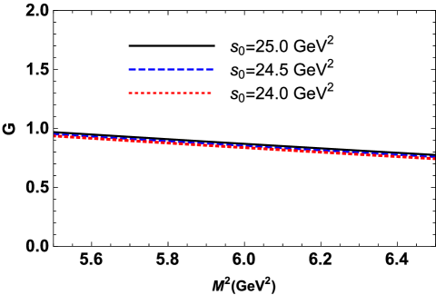
Figure 2: The strong coupling $G$ as a function of the Borel parameter $M^{2}$ at fixed $s_{0}$.

IV Processes $X\to\eta_{c}\eta^{(\prime)}$ and $X\to\chi_{1c}\eta^{(\prime)}$

In this section, we consider processes $X\rightarrow\eta_{c}\eta^{(\prime)}$ and $X\rightarrow\chi_{1c}\eta^{(\prime)}$ and calculate their partial widths. It is not difficult to see, that decays to pseudoscalar mesons $\eta_{c}(1S)$ and $\eta^{(\prime)}$ with spin-parities $J^{\mathrm{PC}}=0^{-+}$ are $P$-wave modes of the tetraquark $X$. The second pair of decays to axial-vector meson $\chi_{1c}(1P)$ with $J^{\mathrm{PC}}=1^{++}$ and $\eta^{(\prime)}$ are its $S$-wave modes. In all of these processes conservation of $C$-parity is the case.

IV.1 Decays $X\rightarrow\eta_{c}\eta$ and $X\rightarrow\eta_{c}\eta^{\prime}$

We start from analysis of the processes $X\rightarrow\eta_{c}\eta$ and $X\rightarrow\eta_{c}\eta^{\prime}$, and extract couplings $g_{1}$ and $g_{2}$ which describe strong interaction at the vertices $X\eta_{c}\eta$ and $X\eta_{c}\eta^{\prime}$, respectively.

The strong coupling $g_{1}$ is defined through on-mass-shell matrix element

$$\langle\eta(q)\eta_{c}\left(p\right)|X(p^{\prime})\rangle=g_{1}p\cdot\varepsilon(p^{\prime}).$$ (54)

The correlation function for analysis of this coupling has the following form

$$\widetilde{\Pi}_{\mu}(p,q)=i\int d^{4}xe^{ipx}\langle\eta(q)|\mathcal{T}\{J^{\eta_{c}}(x)J_{\mu}^{{\dagger}}(0)\}|0\rangle,$$ (55)

where $J^{\eta_{c}}(x)$ is the interpolating current for the $\eta_{c}$ meson

$$J^{\eta_{c}}(x)=\overline{c}_{l}(x)i\gamma_{5}c_{l}(x).$$ (56)

The term which will be used to determine $g_{1}$ is

$$\widetilde{\Pi}_{\mu}^{\mathrm{Phys}}(p,q)=g_{1}\frac{fm_{2}^{2}f_{2}}{4m_{c}m\left(p^{\prime 2}-m^{2}\right)\left(p^{2}-m_{2}^{2}\right)}$$

$$\times\left[(m_{2}^{2}-m_{\eta}^{2}-m^{2})p_{\mu}+(m_{2}^{2}+m_{\eta}^{2}+m^{2})q_{\mu}\right]$$

$$+\cdots.$$ (57)

Here, $m_{2}$ and $m_{\eta}$ are masses of the $\eta_{c}$ and $\eta$ mesons, respectively. The decay constant of the $\eta_{c}$ meson is denoted by $f_{2}$. Let us note that to derive Eq. (57), we use the matrix elements of the tetraquark $X$ from Eq. (6), and the matrix element of the $\eta_{c}$ meson

$$\langle 0|J^{\eta_{c}}|\eta_{c}\left(p\right)\rangle=\frac{f_{2}m_{2}^{2}}{2m_{c}}.$$ (58)

The QCD side of the sum rule reads

$$\widetilde{\Pi}_{\mu}^{\mathrm{OPE}}(p,q)=i\int d^{4}xe^{ipx}\epsilon\widetilde{\epsilon}\left\{\left[\gamma_{5}\widetilde{S}_{c}^{lc}(x)\gamma_{5}\right.\right.$$

$$\left.\left.\times\widetilde{S}_{c}^{el}(-x)\gamma_{\mu}\gamma_{5}\right]+\left[\gamma_{\mu}\gamma_{5}\widetilde{S}_{c}^{lc}(x){}\gamma_{5}\widetilde{S}_{c}^{el}(-x){}\gamma_{5}\right]\right\}_{\alpha\beta}$$

$$\times\langle\eta(q)|\overline{s}_{\alpha}^{b}(0)s_{\beta}^{d}(0)|0\rangle.$$ (59)

It is clear that $\widetilde{\Pi}_{\mu}^{\mathrm{OPE}}(p,q)$ contains only local matrix elements of $\eta$, therefore remaining calculations have to be carried out in the context of the soft-meson approximation. Technical methods of such treatment have been explained in the previous section. Therefore, we do not concentrate on further details, and note that in the soft limit $\widetilde{\Pi}_{\mu}^{\mathrm{OPE}}(p,0)$ receives contributions only from the matrix element

$$2m_{s}\langle\eta|\overline{s}i\gamma_{5}s|0\rangle=h_{\eta}^{s}.$$ (60)

The parameter $h_{\eta}^{s}$ in Eq. (60) can be defined theoretically Agaev:2014wna , but for our purposes it is enough to use its phenomenological value extracted from analysis of relevant exclusive processes. Thus, we have

$$h_{\eta}^{s}=-h_{s}\sin\varphi,\ h_{s}=(0.087\pm 0.006)~{}\mathrm{GeV}^{3},$$ (61)

where $\varphi=39.3^{\circ}\pm 1.0^{\circ}$ is the $\eta-\eta^{\prime}$ mixing angle in the quark-flavor basis (for details, see Ref. Agaev:2014wna ).

The sum rule for $g_{1}$ is derived by making use of invariant amplitudes corresponding to structures $p_{\mu}$ in $\widetilde{\Pi}_{\mu}^{\mathrm{Phys}}(p)$ and $\widetilde{\Pi}_{\mu}^{\mathrm{OPE}}(p)$. It reads

$$g_{1}=\frac{4mm_{c}}{fm_{2}^{2}f_{2}}\frac{\mathcal{P}(M^{2},m^{\prime 2})\mathcal{B}\widetilde{\Pi}^{\mathrm{OPE}}(p^{2})}{m_{2}^{2}-m^{2}-m_{\eta}^{2}},$$ (62)

where $m^{\prime 2}=(m^{2}+m_{2}^{2})/2$. The Borel transformed and subtracted invariant amplitude $\mathcal{B}\widetilde{\Pi}^{\mathrm{OPE}}(p^{2})$ is given by the following expression

$$\mathcal{B}\widetilde{\Pi}^{\mathrm{OPE}}(p^{2}) = -\frac{h_{\eta}^{s}m_{c}}{4\pi^{2}m_{s}}\int_{4\mathcal{M}^{2}}^{s_{0}}ds\frac{\sqrt{s(s-4m_{c}^{2})}}{s}e^{-s/M^{2}}$$ (63)

$$+\widetilde{\Pi}(M^{2}).$$

The nonperturbative component $\widetilde{\Pi}(M^{2})$ is calculated with dimension-$8$ accuracy and determined by formulas similar to ones from Eqs. (45)-(48). Therefore, there is no need to write down their explicit expressions.

The width of the mode $X\rightarrow\eta_{c}\eta$ can be calculated using the formula

$$\Gamma(X\rightarrow\eta_{c}\eta)=g_{1}^{2}\frac{\lambda^{3}(m,m_{2},m_{\eta})}{24\pi m^{2}}.$$ (64)

Numerical computations yield

$$|g_{1}|=3.75\pm 0.78,$$ (65)

and

$$\Gamma(X\rightarrow\eta_{c}\eta)=(18.0\pm 5.4)~{}\mathrm{MeV.}$$ (66)

The second process $X\rightarrow\eta_{c}\eta^{\prime}$ can be considered in a similar manner, difference being in the matrix element of the $\eta^{\prime}$ meson

$$2m_{s}\langle\eta^{\prime}|\overline{s}i\gamma_{5}s|0\rangle=h_{s}\cos\varphi,$$ (67)

that contributes to the corresponding correlation function. For this decay, we find

$$g_{2}=4.38\pm 0.90,$$ (68)

and

$$\Gamma(X\rightarrow\eta_{c}\eta^{\prime})=(15.5\pm 4.5)~{}\mathrm{MeV}.$$ (69)

Effects of these processes on the full width of $X$ are not small, and will be taken into account.

IV.2 Decays $X\rightarrow\chi_{1c}\eta$ and $X\rightarrow\chi_{1c}\eta^{\prime}$

Processes $X\rightarrow\chi_{1c}\eta$ and $X\rightarrow\chi_{1c}\eta^{\prime}$ are explored in accordance with the scheme described above. Here, we have to evaluate the strong couplings $g_{3}$ and $g_{4}$ which correspond to vertices $X\chi_{1c}\eta$ and $X\chi_{1c}\eta^{\prime}$.

Let us consider the decay $X\rightarrow\chi_{1c}\eta$ and write down some principal expressions. The relevant strong coupling $g_{3}$ is defined by the on-mass-shell matrix element

$$\langle\eta(q)\chi_{1c}\left(p\right)|X(p^{\prime})\rangle=g_{3}\left\{\left[p\cdot p^{\prime}\right]\left[\varepsilon^{\ast}(p)\cdot\varepsilon(p^{\prime})\right]\right.$$

$$\left.-[p\cdot\varepsilon(p^{\prime})][p^{\prime}\cdot\varepsilon^{\ast}(p)]\right\},$$ (70)

with $\varepsilon_{\mu}^{\ast}(p)$ being the polarization vector of the meson $\chi_{1c}$.

To determine $g_{3}$, we consider the correlation function

$$\widehat{\Pi}_{\mu\nu}(p,q)=i\int d^{4}xe^{ipx}\langle\eta(q)|\mathcal{T}\{J_{\nu}^{\chi_{1c}}(x)J_{\mu}^{{\dagger}}(0)\}|0\rangle,$$ (71)

where $J_{\mu}^{\chi_{1c}}(x)$ is the interpolating current for the axial-vector meson $\chi_{1c}$

$$J_{\nu}^{\chi_{1c}}(x)=\overline{c}_{l}(x)i\gamma_{5}\gamma_{\nu}c_{l}(x).$$ (72)

Then, the term in $\widehat{\Pi}_{\mu\nu}(p,q)$ which has two poles in variables $p^{2}$ and $p^{\prime 2}=(p+q)^{2}$ is given by the formula

$$\widehat{\Pi}_{\mu\nu}^{\mathrm{Phys}}(p,q)=g_{3}\frac{fmf_{3}m_{3}}{\left(p^{\prime 2}-m^{2}\right)\left(p^{2}-m_{3}^{2}\right)}$$

$$\times\left[\frac{1}{2}\left(m^{2}+m_{3}^{2}-m_{\eta}^{2}\right)g_{\mu\nu}-p_{\mu}p_{\nu}^{\prime}\right]$$

$$+\cdots,$$ (73)

where $m_{3}$ and $f_{3}$ are the mass and decay constant of the $\chi_{1c}$ meson. As usual, dots stand for contributions of higher resonances and continuum states. The ground-state term in $\widehat{\Pi}_{\mu\nu}^{\mathrm{Phys}}(p,q)$ has been found using the matrix element

$$\langle 0|J_{\mu}^{\chi_{1c}}|\chi_{1c}\left(p\right)\rangle=f_{3}m_{3}\varepsilon_{\mu}(p),$$ (74)

as well as matrix element of the tetraquark $X$.

The correlation function $\widehat{\Pi}_{\mu\nu}^{\mathrm{OPE}}(p,q)$ is given by the expression

$$\widehat{\Pi}_{\mu\nu}^{\mathrm{OPE}}(p,q)=i\int d^{4}xe^{ipx}\epsilon\widetilde{\epsilon}\left\{\left[\gamma_{5}\widetilde{S}_{c}^{lc}(x)\gamma_{\nu}\gamma_{5}\right.\right.$$

$$\left.\left.\times\widetilde{S}_{c}^{el}(-x)\gamma_{\mu}\gamma_{5}\right]+\left[\gamma_{\mu}\gamma_{5}\widetilde{S}_{c}^{lc}(x){}\gamma_{\nu}\gamma_{5}\widetilde{S}_{c}^{el}(-x){}\gamma_{5}\right]\right\}_{\alpha\beta}$$

$$\times\langle\eta(q)|\overline{s}_{\alpha}^{b}(0)s_{\beta}^{d}(0)|0\rangle.$$ (75)

The required sum rule for the coupling $g_{3}$ is derived by equating invariant amplitudes of structures $\sim g_{\mu\nu}$ from the functions $\widehat{\Pi}_{\mu\nu}^{\mathrm{Phys}}(p,q)$ and $\widehat{\Pi}_{\mu\nu}^{\mathrm{OPE}}(p,q)$, and has the form

$$g_{3}=\frac{2}{fmf_{3}m_{3}}\frac{\mathcal{P}(M^{2},\widehat{m}^{2})\mathcal{B}\widehat{\Pi}^{\mathrm{OPE}}(p^{2})}{2\widehat{m}^{2}-m_{\eta}^{2}},$$ (76)

where $\widehat{m}^{2}=(m^{2}+m_{3}^{2})/2$. Numerical analysis for $g_{3}$ gives

$$g_{3}=(1.34\pm 0.23)\times 10^{-1}~{}\mathrm{GeV}^{-1}.$$ (77)

Width of the process $X\rightarrow\chi_{1c}\eta$ is determined by the expression

$$\Gamma(X\rightarrow\chi_{1c}\eta)=g_{3}^{2}\frac{\lambda m_{3}^{2}}{24\pi}\left(3+\frac{2\lambda^{2}}{m_{3}^{2}}\right),$$ (78)

with $\lambda$ being equal to $\lambda(m,m_{3},m_{\eta})$. Then it is not difficult to find that

$$\Gamma(X\rightarrow\chi_{1c}\eta)=(7.9\pm 1.9)~{}\mathrm{MeV}.$$ (79)

For the decay $X\rightarrow\chi_{1c}\eta^{\prime}$, we get

$$|g_{4}|=(1.39\pm 0.23)\times 10^{-1}~{}\mathrm{GeV}^{-1},$$ (80)

and

$$\Gamma(X\rightarrow\chi_{1c}\eta^{\prime})=(4.9\pm 1.2)\ \ \mathrm{MeV},$$ (81)

respectively.

V Summing up

The full width of the tetraquark $X$ can be evaluated using results for the partial width of its five decay modes obtained in Sections III and IV. One of these modes $X\rightarrow J/\psi\phi$ is the dominant decay channel of the tetraquark $X$, whereas remaining processes are sub-dominant ones. After simple computations, we get

$$\Gamma=(159\pm 31)~{}\mathrm{MeV}.$$ (82)

Our result for the full width $\Gamma$ of the tetraquark $X$ is in a very nice agreement with $\Gamma_{\exp}=(174\pm 27_{-73}^{+134})~{}\mathrm{MeV}$ found by the LHCb collaboration.

But by drawing such conclusions, we take into account that both theoretical and experimental information on the full with of $X(4630)$ suffers from errors. The uncertainties are large in the case of  $\Gamma_{\exp}$ which limit credibility of conclusions that are based on these data. Experimental errors also make it difficult to obtain detailed comparisons and choices between existing theoretical models for $X(4630)$. In this sense, more precise measurements of $\Gamma_{\exp}$ are required.

From another side, our present result can be further refined by including into analysis other decay modes of $X$. There are a few processes which contribute to the full width of the tetraquark $X$. Thus, decays to meson pairs $D_{s}^{\ast\pm}D_{s0}(2317)^{\mp}$ and $D_{s}^{\pm}D_{s1}(2460)^{\mp}$ are among kinematically allowed channels of $X$ . These processes belong to $\mathrm{V\rightarrow V+S}$ and $\mathrm{V\rightarrow PS+AV}$ type $S$-wave decay modes of $X$, respectively. Their partial widths are determined by the expression Eq. (78) with relevant strong coupling. To make crude estimates for partial widths of these decays, we may assume that strong couplings at corresponding tetraquark-meson-meson vertices are a same order of $g_{3}$ ($|g_{4}|$). Then widths of these modes are suppressed relative to decays $X\rightarrow\chi_{1c}\eta^{(\prime)}$, because the factor $\Lambda=m_{\ast}^{2}$ $\lambda\left(3+2\lambda^{2}/m_{\ast}^{2}\right)/24\pi$ ($m_{\ast}$ is a mass of a heaviest final meson) is smaller for two final-state mesons of approximately equal mass than in the case of light and heavy mesons. For instance, in the decay $X\rightarrow\chi_{1c}\eta$ it is equal to $\Lambda\approx 0.44$, while we find $\Lambda\approx 0.17$ for the process $X\rightarrow D_{s}^{-}D_{s1}(2460)^{+}$. But these decay channels, in total, may compensate a $15~{}\mathrm{MeV}$ gap between $\Gamma_{\exp}$ and $\Gamma$.

Another interesting field of future studies is an exploration of $X(4630)$ in the molecule picture using the QCD sum rule method. This is necessary to compare predictions for the molecule and diquark-antidiquark models with each another, as well as with the LHCb data. In the context of the QCD sum rule approach diquark-antidiquark and molecule models for the same resonance lead to different results Agaev:2021vur ; Agaev:2022ast . As a rule, a molecule of conventional mesons is heavier than a diquark-antidiquark structure with identical content and spin-parities. A width of such molecule is also larger than that of its diquark counterpart, i.e., a diquark structure is more stable than a meson molecule. Nevertheless, despite existing investigations of $X(4630)$ in different approaches, it is necessary to examine the molecule model for $X(4630)$ in the context of the QCD sum rule method as well.

Analysis performed in the present article and gained knowledge about the mass and full width of the tetraquark $X$, as well as a very nice agreement between these parameters and LHCb measurements allows us to interpret $X(4630)$ as the vector diquark-antidiquark state $X$ with the spin-parities $J^{\mathrm{PC}}=1^{-+}$.

Appendix A The quark propagators and invariant amplitude $\Pi(M^{2},s_{0})$

In the current article, for the light quark propagator $S_{q}^{ab}(x)$, we employ the following expression

$$S_{q}^{ab}(x)=i\delta_{ab}\frac{\not{x}}{2\pi^{2}x^{4}}-\delta_{ab}\frac{m_{q}}{4\pi^{2}x^{2}}-\delta_{ab}\frac{\langle\overline{q}q\rangle}{12}+i\delta_{ab}\frac{\not{x}m_{q}\langle\overline{q}q\rangle}{48}-\delta_{ab}\frac{x^{2}}{192}\langle\overline{q}g_{s}\sigma Gq\rangle$$

$$+i\delta_{ab}\frac{x^{2}\not{x}m_{q}}{1152}\langle\overline{q}g_{s}\sigma Gq\rangle-i\frac{g_{s}G_{ab}^{\alpha\beta}}{32\pi^{2}x^{2}}\left[\not{x}{\sigma_{\alpha\beta}+\sigma_{\alpha\beta}}\not{x}\right]-i\delta_{ab}\frac{x^{2}\not{x}g_{s}^{2}\langle\overline{q}q\rangle^{2}}{7776}$$

$$-\delta_{ab}\frac{x^{4}\langle\overline{q}q\rangle\langle g_{s}^{2}G^{2}\rangle}{27648}+\cdots.$$ (A.83)

For the heavy quark $Q=c$, we use the propagator $S_{Q}^{ab}(x)$

$$S_{Q}^{ab}(x)=i\int\frac{d^{4}k}{(2\pi)^{4}}e^{-ikx}\Bigg{\{}\frac{\delta_{ab}\left({\not{k}}+m_{Q}\right)}{k^{2}-m_{Q}^{2}}-\frac{g_{s}G_{ab}^{\alpha\beta}}{4}\frac{\sigma_{\alpha\beta}\left({\not{k}}+m_{Q}\right)+\left({\not{k}}+m_{Q}\right)\sigma_{\alpha\beta}}{(k^{2}-m_{Q}^{2})^{2}}$$

$$+\frac{g_{s}^{2}G^{2}}{12}\delta_{ab}m_{Q}\frac{k^{2}+m_{Q}{\not{k}}}{(k^{2}-m_{Q}^{2})^{4}}+\frac{g_{s}^{3}G^{3}}{48}\delta_{ab}\frac{\left({\not{k}}+m_{Q}\right)}{(k^{2}-m_{Q}^{2})^{6}}\left[{\not{k}}\left(k^{2}-3m_{Q}^{2}\right)+2m_{Q}\left(2k^{2}-m_{Q}^{2}\right)\right]\left({\not{k}}+m_{Q}\right)+\cdots\Bigg{\}}.$$

Here, we have used the short-hand notations

$$G_{ab}^{\alpha\beta}\equiv G_{A}^{\alpha\beta}\lambda_{ab}^{A}/2,\ \ G^{2}=G_{\alpha\beta}^{A}G_{A}^{\alpha\beta},\ G^{3}=f^{ABC}G_{\alpha\beta}^{A}G^{B\beta\delta}G_{\delta}^{C\alpha},$$ (A.85)

where $G_{A}^{\alpha\beta}$ is the gluon field strength tensor, $\lambda^{A}$ and $f^{ABC}$ are the Gell-Mann matrices and structure constants of the color group $SU_{c}(3)$, respectively. The indices $A,B,C$ run in the range $1,2,\ldots 8$.

The invariant amplitude $\Pi(M^{2},s_{0})$ obtained after the Borel transformation and subtraction procedures is given by the expression

$$\Pi(M^{2},s_{0})=\int_{4\mathcal{M}^{2}}^{s_{0}}ds\rho^{\mathrm{OPE}}(s)e^{-s/M^{2}}+\Pi(M^{2}),$$

where the spectral density $\rho^{\mathrm{OPE}}(s)$ and the function $\Pi(M^{2})$ are determined by formulas

$$\rho^{\mathrm{OPE}}(s)=\rho^{\mathrm{pert.}}(s)+\sum_{N=3}^{8}\rho^{\mathrm{DimN}}(s),\ \ \Pi(M^{2})=\sum_{N=6}^{10}\Pi^{\mathrm{DimN}}(M^{2}),$$ (A.86)

respectively. The components of $\rho^{\mathrm{OPE}}(s)$ and $\Pi(M^{2})$ are given by the expressions

$$\rho^{\mathrm{DimN}}(s)=\int_{0}^{1}d\alpha\int_{0}^{1-a}d\beta\rho^{\mathrm{DimN}}(s,\alpha,\beta),\ \ \Pi^{\mathrm{DimN}}(M^{2})=\int_{0}^{1}d\alpha\int_{0}^{1-a}d\beta\Pi^{\mathrm{DimN}}(M^{2},\alpha,\beta),$$ (A.87)

if $\rho^{\mathrm{DimN}}(s,\alpha,\beta)$ and $\Pi^{\mathrm{DimN}}(M^{2},\alpha,\beta)$ are functions of $\alpha$ and $\beta$, and by formulas

$$\rho^{\mathrm{DimN}}(s)=\int_{0}^{1}d\alpha\rho^{\mathrm{DimN}}(s,\alpha),\ \ \Pi^{\mathrm{DimN}}(M^{2})=\int_{0}^{1}d\alpha\Pi^{\mathrm{DimN}}(M^{2},\alpha),$$ (A.88)

provided that they depend only on $\alpha$. Let us note that in Eqs. (A.87) and (A.88) variables $\alpha$ and $\beta$ are Feynman parameters.

The perturbative and nonperturbative components of the spectral density $\rho^{\mathrm{pert.}}(s,\alpha,\beta)$ and $\rho^{\mathrm{Dim3(4,5,6,7,8)}}(s,\alpha,\beta)$  have the forms:

$$\rho^{\mathrm{pert.}}(s,\alpha,\beta)=\frac{\Theta(L_{1})}{1536\pi^{6}L^{2}N_{1}^{8}}\left[m_{c}^{2}N_{2}-s\alpha\beta L\right]^{2}\left\{12m_{c}^{3}m_{s}L(\alpha+\beta)^{2}N_{1}^{3}-m_{c}^{4}\alpha\beta N_{1}^{2}\left[5\beta^{3}+5\alpha^{2}(\alpha-1)\right.\right.$$

$$\left.+\alpha\beta(-10+13\alpha)+\beta^{2}(-5+13\alpha)\right]-35s^{2}\alpha^{3}\beta^{3}L^{3}-12m_{c}m_{s}s\alpha\beta(\alpha+\beta)\left[\beta^{3}+2\beta^{2}(\alpha-1)+\alpha(\alpha-1)^{2}\right.$$

$$\left.+\beta(1-3\alpha+2\alpha^{2})\right]^{2}+2m_{c}^{2}s\alpha^{2}\beta^{2}\left[\beta^{3}+2\beta^{2}(\alpha-1)+\alpha(\alpha-1)^{2}+\beta(1-3\alpha+2\alpha^{2})\right]\left[14\beta^{2}+14\alpha(\alpha-1)\right.$$

$$\left.\left.+\beta(-14+27\alpha)\right]\right\},$$ (A.89)

$$\rho^{\mathrm{Dim3}}(s,\alpha,\beta)=-\frac{\langle\overline{s}s\rangle\Theta(L_{1})}{16\pi^{4}N_{1}^{6}}\left\{m_{c}^{5}N_{2}^{3}-m_{s}s^{2}\alpha^{2}\beta^{2}L^{3}\left[\beta^{2}+\alpha(\alpha-1)-\beta(1+14\alpha)\right]+m_{c}s^{2}\alpha^{2}\beta^{2}L^{2}N_{2}\right.$$

$$-2m_{c}^{3}s\alpha\beta LN_{2}^{2}+3m_{c}^{4}m_{s}N_{1}^{2}\left[\beta^{5}+\alpha^{3}(\alpha-1)^{2}+\beta^{4}(-2+4\alpha)+\beta\alpha^{2}(3-7\alpha+4\alpha^{2})+\beta^{2}\alpha(3-10\alpha+8\alpha^{2})\right.$$

$$\left.+\beta^{3}(1-7\alpha+8\alpha^{2})\right]-sm_{c}^{2}m_{s}\alpha\beta\left[2\beta^{7}+2\alpha^{3}(\alpha-1)^{4}-\beta^{6}(8-23\alpha)+\beta\alpha^{2}(\alpha-1)^{3}(-6+23\alpha)\right.$$

$$+\beta^{5}(12-75\alpha+79\alpha^{2})+\beta^{2}\alpha(\alpha-1)^{2}(6-54\alpha+79\alpha^{2})+\beta^{4}(-8+87\alpha-212\alpha^{2}+133\alpha^{3})$$

$$\left.\left.+\beta^{3}(2-41\alpha+193\alpha^{2}-287\alpha^{3}+133\alpha^{4})\right]\right\},$$ (A.90)

$$\rho^{\mathrm{Dim4}}(s,\alpha,\beta)=-\frac{\langle\alpha_{s}G^{2}/\pi\rangle\Theta(L_{1})}{9216\pi^{4}L^{2}N_{1}^{6}}\left\{-15s^{2}\alpha^{3}\beta^{3}L^{4}(9\beta+4\alpha)+m_{c}^{4}\alpha\beta N_{1}^{2}\left[2\beta^{5}+\beta^{4}(28-82\alpha)+\beta^{2}\alpha\left(-72\right.\right.\right.$$

$$\left.\left.+255\alpha-163\alpha^{2}\right)+\beta\alpha^{2}(-54+97\alpha-19\alpha^{2})+4\alpha^{3}(-3-2\alpha+5\alpha^{2})-2\beta^{3}(15-89\alpha+104\alpha^{2})\right]$$

$$+6sm_{c}m_{s}\alpha\beta L^{2}\left[5\beta^{7}+2\alpha^{4}(\alpha-1)^{2}(3+\alpha)-2\beta\alpha^{3}(\alpha-1)^{2}(-28+31\alpha)-\beta^{6}(7+53\alpha)-\beta^{2}\alpha^{2}(\alpha-1)^{2}\right.$$

$$\left.\times(-97+173\alpha)+\beta^{5}(-1+156\alpha-161\alpha^{2})+\beta^{3}\alpha(50-355\alpha+588\alpha^{2}-283\alpha^{3})+\beta^{4}(3-153\alpha+419\alpha^{2}-277\alpha^{3})\right]$$

$$-6m_{c}^{3}m_{s}N_{1}^{2}\left[5\beta^{7}+2\alpha^{4}(\alpha-1)^{2}(3+\alpha)-\beta^{6}(7+26\alpha)+\beta^{5}(-1+96\alpha-143\alpha^{2})+\beta^{4}(3-106\alpha+356\alpha^{2}-259\alpha^{3})\right.$$

$$\left.+\beta^{2}\alpha^{2}(69-297\alpha+389\alpha^{2}-161\alpha^{3})+2\beta^{3}\alpha(18-141\alpha+255\alpha^{2}-134\alpha^{3})-2\beta\alpha^{3}(-21+65\alpha-63\alpha^{2}+19\alpha^{3})\right]$$

$$+m_{c}^{2}s\alpha^{2}\beta^{2}\left[\beta^{3}+2\beta^{2}(\alpha-1)+\alpha(\alpha-1)^{2}+\beta(1-3\alpha+2\alpha^{2})\right]\left[75\beta^{4}+3\beta^{3}(-74+149\alpha)-12\alpha^{2}(-5+4\alpha+\alpha^{2})\right.$$

$$\left.\left.+\alpha\beta(207-535\alpha+264\alpha^{2})+\beta^{2}(147-718\alpha+627\alpha^{2})\right]\right\},$$ (A.91)

$$\rho_{1}^{\mathrm{Dim5}}(s,\alpha,\beta)=\frac{\langle\overline{s}g_{s}\sigma Gs\rangle\Theta(L_{1})L}{96\pi^{4}N_{1}^{5}}\left\{-16sm_{s}\alpha^{2}\beta^{2}L^{2}+3m_{c}^{3}N_{2}^{2}-3sm_{c}\alpha\beta\left[\beta^{4}+\alpha^{2}(\alpha-1)^{2}+\beta^{3}(-2+3\alpha)\right.\right.$$

$$\left.+\alpha\beta(2-5\alpha+3\alpha^{2})+\beta^{2}(1-5\alpha+4\alpha^{2})\right]+m_{c}^{2}m_{s}\alpha\beta\left[7\beta^{4}+7\alpha^{2}(\alpha-1)^{2}+2\beta^{3}(-7+10\alpha)\right.$$

$$\left.\left.+2\alpha\beta(7-17\alpha+10\alpha^{2})+\beta^{2}(7-34\alpha+27\alpha^{2})\right]\right\},$$ (A.92)

$$\rho_{1}^{\mathrm{Dim6}}(M^{2},\alpha,\beta)=-\frac{\Theta(L_{1})}{405\cdot 2^{12}\pi^{6}(\beta-1)^{2}L^{2}N_{1}^{7}}\left\{2560g_{s}^{2}\pi^{2}\langle\overline{s}s\rangle^{2}(\beta-1)^{2}\alpha\beta L^{3}N_{1}^{2}\left[-16s\alpha\beta L^{2}+m_{c}^{2}\left(7\beta^{4}+7\alpha^{2}\right.\right.\right.$$

$$\left.\left.\times(\alpha-1)^{2}+2\beta^{3}(-7+10\alpha)+2\beta\alpha(7-17\alpha+10\alpha^{2})+\beta^{2}(7-34\alpha+27\alpha^{2})\right)\right]+9\langle g_{s}^{3}G^{3}\rangle\left[-18m_{c}m_{s}(\beta-1)^{2}N_{1}^{2}\right.$$

$$\left(3\beta^{9}+\beta^{8}(-9+\alpha)-3\beta^{3}\alpha^{5}(\alpha-1)-5\beta^{2}\alpha^{5}(\alpha-1)^{2}+3\alpha^{6}(\alpha-1)^{3}+\beta^{7}(9-5\alpha^{2})+\beta^{5}\alpha(2-5\alpha+3\alpha^{2})\right.$$

$$\left.+\beta\alpha^{5}(2-3\alpha+\alpha^{3})-\beta^{6}(3+3\alpha-10\alpha^{2}+3\alpha^{3})\right)+3m_{c}^{2}\alpha\beta\left(17\beta^{13}+2\beta^{12}(-51+19\alpha)-\alpha^{7}(\alpha-1)^{4}(-17-2\alpha+\alpha^{2})\right.$$

$$+\beta^{11}(255-214\alpha+37\alpha^{2})-\beta^{10}(340-500\alpha+182\alpha^{2}+\alpha^{3})-\beta^{2}\alpha^{5}(\alpha-1)^{3}(-3-79\alpha+65\alpha^{2}+4\alpha^{3})-\beta\alpha^{6}(\alpha-1)^{3}$$

$$\times(24-66\alpha+20\alpha^{2}+7\alpha^{3})-\beta^{3}\alpha^{4}(\alpha-1)^{2}(10-35\alpha-63\alpha^{2}+71\alpha^{3})+\beta^{9}(255-620\alpha+355\alpha^{2}+31\alpha^{3}-41\alpha^{4})$$

$$-\beta^{4}\alpha^{3}(\alpha-1)^{2}(10-66\alpha+107\alpha^{2}-17\alpha^{3}+9\alpha^{4})-2\beta^{8}\left(51-215\alpha+170\alpha^{2}+62\alpha^{3}-105\alpha^{4}+30\alpha^{5}\right)$$

$$+\beta^{7}(17-158\alpha+155\alpha^{2}+206\alpha^{3}-440\alpha^{4}+282\alpha^{4}-66\alpha^{6})+\beta^{6}\alpha\left(24-22\alpha-169\alpha^{2}+480\alpha^{3}-532\alpha^{4}+281\alpha^{5}\right.$$

$$\left.\left.-62\alpha^{6}\right)+\beta^{5}\alpha^{2}\left(-3+67\alpha-285\alpha^{2}+507\alpha^{3}-449\alpha^{4}+202\alpha^{5}-39\alpha^{6}\right)\right)+2s\alpha^{2}\beta^{2}L^{2}\left(21\beta^{9}-4\beta^{8}(21+8\alpha)\right.$$

$$+\beta^{7}(126+128\alpha-28\alpha^{2})-3\alpha^{5}(\alpha-1)^{2}(-7-2\alpha+\alpha^{2})-4\beta\alpha^{4}(\alpha-1)^{2}(8+9\alpha+3\alpha^{2})$$

$$+4\beta^{6}(-21-48\alpha+20\alpha^{2}+3\alpha^{3})+\beta^{4}\alpha(-32+16\alpha+48\alpha^{2}-31\alpha^{4})+2\beta^{2}\alpha^{3}\left(2+44\alpha-75\alpha^{2}+26\alpha^{3}+3\alpha^{4})\right.$$

$$\left.\left.\left.-4\beta^{3}\alpha^{2}(-1+6\alpha+17\alpha^{2}-33\alpha^{3}+11\alpha^{4})+\beta^{5}(21+128\alpha-72\alpha^{2}-4\alpha^{3}+12\alpha^{4})\right)\right]\right\},$$ (A.93)

$$\rho_{1}^{\mathrm{Dim7}}(M^{2},\alpha,\beta)=-\frac{\langle\alpha_{s}G^{2}/\pi\rangle\langle\overline{s}s\rangle\Theta(L_{1})}{1152\pi^{2}N_{1}^{4}}\left\{9m_{s}\beta\alpha^{2}L^{2}+2m_{c}\left[5\beta^{5}-2\beta^{4}(1+11\alpha)+\beta^{3}(-3+37\alpha-37\alpha^{2})\right.\right.$$

$$\left.\left.+\beta^{2}\alpha(-15+48\alpha-37\alpha^{2})+\beta\alpha^{2}(-15+37\alpha-22\alpha^{2})+\alpha^{3}(-3-2\alpha+5\alpha^{2})\right]\right\},$$ (A.94)

$$\rho_{1}^{\mathrm{Dim8}}(M^{2},\alpha,\beta)=\frac{5\langle\alpha_{s}G^{2}/\pi\rangle^{2}}{3072\pi^{2}N_{1}^{4}}\Theta(L_{1})\alpha^{2}\beta^{2}L.$$ (A.95)

The spectral densities $\rho^{\mathrm{Dim5(6,7,8)}}(s,\alpha)$ are given by the formulas

$$\rho_{1}^{\mathrm{Dim5}}(s,\alpha)=-\frac{6\langle\overline{s}g_{s}\sigma Gs\rangle m_{c}^{2}m_{s}}{96\pi^{4}}\Theta(L_{2}),\ \$$ (A.96)

$$\rho_{2}^{\mathrm{Dim6}}(s,\alpha)=-\frac{\langle\overline{s}s\rangle^{2}}{1296\pi^{4}}\Theta(L_{2})\left[2g_{s}^{2}m_{c}m_{s}+27\pi^{2}(8m_{c}^{2}-4m_{c}m_{s})\right],\ \$$ (A.97)

$$\rho_{2}^{\mathrm{Dim7}}(s,\alpha)=\frac{\langle\alpha_{s}G^{2}/\pi\rangle\langle\overline{s}s\rangle}{288\pi^{2}}\Theta(L_{2})\left[m_{c}-m_{s}\alpha(\alpha-1)\right],\$$ (A.98)

and

$$\rho_{2}^{\mathrm{Dim8}}(s,\alpha)=\frac{\langle\overline{s}s\rangle\langle\overline{s}g_{s}\sigma Gs\rangle}{24\pi^{2}}\Theta(L_{2})\alpha(\alpha-1).\$$ (A.99)

Components of the function $\Pi(M^{2})$ are:

$$\Pi^{\mathrm{Dim6}}(M^{2},\alpha,\beta)=\frac{\langle g_{s}^{3}G^{3}\rangle m_{s}}{15\cdot 2^{13}\pi^{6}M^{2}\alpha^{2}\beta^{2}L^{3}N_{1}^{5}}\left\{2m_{c}M^{2}\alpha^{4}\beta^{4}L^{4}(3\beta^{2}+\beta\alpha+\alpha^{2})-\exp\left[-\frac{m_{c}^{2}N_{2}}{M^{2}\alpha\beta L}\right]\right.$$

$$\times\left[m_{c}^{5}N_{1}^{2}\left(2\beta^{10}+15\beta\alpha^{7}(\alpha-1)^{2}+2\alpha^{8}(\alpha-1)^{2}+\beta^{9}(-4+15\alpha)+\beta^{5}\alpha^{3}(-15+80\alpha-74\alpha^{2})\right.\right.$$

$$+2\beta^{6}\alpha^{2}(6+9\alpha-26\alpha^{2})+\beta^{7}\alpha(15-32\alpha-3\alpha^{2})-3\beta^{3}\alpha^{5}(5-6\alpha+\alpha^{2})+4\beta^{2}\alpha^{6}(3-8\alpha+5\alpha^{2})$$

$$\left.-4\beta^{4}\alpha^{4}(7-20\alpha+13\alpha^{2})+\beta^{8}(2-30\alpha+20\alpha^{2})\right)-2m_{c}^{3}M^{2}\alpha^{2}\beta^{2}L^{2}\left(2\beta^{8}-5\beta\alpha^{5}(\alpha-1)^{2}+2\alpha^{6}(\alpha-1)^{2}\right.$$

$$-\beta^{7}(4+5\alpha)+\beta^{5}\alpha(-5+38\alpha-44\alpha^{2})+\beta^{6}(2+10\alpha-20\alpha^{2})-22\beta^{3}\alpha^{3}(1-3\alpha+2\alpha^{2})$$

$$\left.\left.\left.-2\beta^{2}\alpha^{4}(9-19\alpha+10\alpha^{2})-2\beta^{4}\alpha^{2}(9-33\alpha+26\alpha^{2})\right)\right]\right\},$$ (A.100)

$$\Pi^{\mathrm{Dim7}}(M^{2},\alpha,\beta)=\frac{\langle\alpha_{s}G^{2}/\pi\rangle\langle\overline{s}s\rangle m_{c}^{2}m_{s}}{72\pi^{2}LN_{1}^{3}}\left[\beta^{4}+\alpha^{2}(\alpha-1)^{2}+\beta^{3}(-2+3\alpha)+\alpha\beta(2-5\alpha+\alpha^{2})\right.$$

$$\left.+\alpha\beta(2-5\alpha+\alpha^{2})+\beta^{2}(1-5\alpha+4\alpha^{2})\right],$$ (A.101)

$$\Pi^{\mathrm{Dim8}}(M^{2},\alpha,\beta)=-\frac{\langle\alpha_{s}G^{2}/\pi\rangle^{2}m_{c}}{81\cdot 2^{10}\pi^{2}M^{6}\alpha\beta(\beta-1)L^{6}N_{1}^{3}}\exp\left[-\frac{m_{c}^{2}N_{2}}{M^{2}\alpha\beta L}\right]\left\{24m_{c}^{4}m_{s}M^{2}(\beta-1)(\alpha+\beta)^{3}L^{4}N_{1}^{2}\right.$$

$$+6m_{c}^{7}(\alpha+\beta)^{2}N_{1}^{5}-60m_{s}M^{6}\alpha\beta(\beta-1)L^{5}\left[\beta^{4}-\beta^{3}+\alpha^{3}(\alpha-1)\right]-9m_{c}M^{6}\alpha^{2}\beta^{2}(\beta-1)(\alpha^{2}+\beta^{2})L^{5}$$

$$-6m_{c}^{2}m_{s}M^{4}(\beta-1)L^{4}\left[8\beta^{7}+18\beta\alpha^{4}(\alpha-1)^{2}+8\alpha^{5}(\alpha-1)^{2}+2\beta^{6}(-8+9\alpha)+7\beta^{2}\alpha^{3}(2-5\alpha+3\alpha^{2})\right.$$

$$\left.+2\beta^{3}\alpha^{2}(7-15\alpha+8\alpha^{2})+\beta^{4}\alpha(18-35\alpha+16\alpha^{2})+\beta^{5}(8-36\alpha+21\alpha^{2})\right]-2m_{c}^{5}M^{2}\left[12\beta^{7}-3\beta^{8}+3\alpha^{4}\right.$$

$$\times(\alpha-1)^{3}+\beta^{6}(-18+6\alpha+\alpha^{2})+3\beta\alpha^{3}(\alpha-1)^{2}(-2+\alpha+3\alpha^{2})+2\beta^{5}(6-9\alpha+8\alpha^{2})$$

$$+\beta^{2}\alpha^{2}(-6+14\alpha+11\alpha^{2}-43\alpha^{3}+24\alpha^{4})+\beta^{4}(-3+18\alpha-9\alpha^{2}-30\alpha^{3}+28\alpha^{4})+\beta^{3}\alpha\left(-6+14\alpha+6\alpha^{2}\right.$$

$$\left.\left.-51\alpha^{3}+37\alpha^{4}\right)\right]\left[\beta^{4}+\alpha^{2}(\alpha-1)^{2}+\beta^{3}(-2+3\alpha)+\beta\alpha(2-5\alpha+3\alpha^{2})+\beta^{2}(1-5\alpha+4\alpha^{2})\right]+m_{c}^{3}M^{4}\alpha\beta L^{2}$$

$$\times\left[-3\beta^{8}+3\alpha^{4}(\alpha-1)^{3}+2\beta^{7}(6+13\alpha)+6\beta^{6}(-3-15\alpha+14\alpha^{2})+\beta\alpha^{3}(\alpha-1)^{2}(12-23\alpha+21\alpha^{2})\right.$$

$$+\beta^{5}(12+114\alpha-289\alpha^{2}+177\alpha^{3})+\beta^{2}\alpha^{2}(30-163\alpha+303\alpha^{2}-244\alpha^{3}+74\alpha^{4})$$

$$\left.\left.+\beta^{3}\alpha(12-181\alpha+467\alpha^{2}-454\alpha^{3}+156\alpha^{4})+\beta^{4}(-3-62\alpha+356\alpha^{2}-493\alpha^{3}+201\alpha^{4})\right]\right\},$$ (A.102)

$$\Pi^{\mathrm{Dim9}}(M^{2},\alpha,\beta)=\frac{\langle\alpha_{s}G^{2}/\pi\rangle\langle\overline{s}g_{s}\sigma Gs\rangle m_{c}N_{1}^{2}}{4608\pi^{2}M^{4}\beta^{4}\alpha^{2}(\beta-1)^{3}L^{4}}\exp\left[-\frac{m_{c}^{2}N_{2}}{M^{2}\alpha\beta L}\right]\left\{48M^{4}\beta^{3}(\beta-1)^{2}\alpha^{2}(\alpha-1)L^{3}+6M^{4}\beta^{3}\alpha\right.$$

$$\times(\beta-1)^{2}L^{3}+121M^{2}m_{c}m_{s}\beta^{2}(\beta-1)\alpha\left(\alpha-1\right)L^{2}N_{1}^{2}+40M^{2}m_{c}m_{s}\beta^{2}(\beta-1)L^{2}N_{1}^{2}-64M^{2}m_{c}m_{s}\beta\alpha^{2}LN_{1}^{4}$$

$$\left.+32M^{2}m_{c}m_{s}\beta\alpha LN_{1}^{4}\left(1+\alpha\right)+16m_{c}^{3}m_{s}(\alpha+\beta)N_{1}^{5}\left(\alpha^{2}-1\right)+32m_{c}^{3}m_{s}\alpha(\alpha+\beta)N_{1}^{5}\right\},$$ (A.103)

and

$$\Pi^{\mathrm{Dim10}}(M^{2},\alpha,\beta)=-\frac{\langle\alpha_{s}G^{2}/\pi\rangle\langle\overline{s}s\rangle^{2}m_{c}^{2}N_{1}^{4}}{729\cdot 2^{5}M^{4}\pi^{2}\alpha^{2}\beta^{4}(\beta-1)^{3}L^{4}}\exp\left[-\frac{m_{c}^{2}N_{2}}{M^{2}\alpha\beta L}\right]\left\{216m_{c}^{2}\pi^{2}(\alpha-1)^{2}(\alpha+\beta)N_{1}^{3}-M^{2}\beta L\right.$$

$$\times\left[-g_{s}^{2}\alpha\beta(\alpha-1)(\beta-1)L+108\pi^{2}\left(4\beta^{4}\alpha(\alpha-1)^{2}+4\alpha^{3}(\alpha-1)^{4}+\beta^{3}(5-23\alpha+39\alpha^{2}-24\alpha^{3}+8\alpha^{4})\right.\right.$$

$$\left.\left.\left.+\beta^{2}(-10+39\alpha-69\alpha^{2}+63\alpha^{3}-40\alpha^{4}+12\alpha^{5})+\beta(5-20\alpha+38\alpha^{2}-47\alpha^{3}+48\alpha^{4}-32\alpha^{5}+8\alpha^{6})\right)\right]\right\}.$$

In expressions above, $\Theta(z)$ is Unit Step function. We have also used the following short-hand notations:

$$N_{1} = \beta^{2}+\beta(\alpha-1)+\alpha(\alpha-1),\ \ \ \ \ N_{2}=(\alpha+\beta)N_{1},\ L=\alpha+\beta-1,\$$

$$\ \ \ L_{1} \equiv L_{1}(s,\alpha,\beta)=\frac{(1-\beta)}{N_{1}^{2}}\left[m_{c}^{2}N_{2}-s\alpha\beta L\right],\ L_{2}\equiv L_{2}(s,\alpha)=s\alpha(1-\alpha)-m_{c}^{2},\$$ (A.105)

References

(1) R. Aaij et al. [LHCb Collaboration],
Phys. Rev. Lett. 127, 082001 (2021).
(2) R. Aaij et al. [LHCb Collaboration],
Phys. Rev. Lett. 118, 022003 (2017).
(3) R. Aaij et al. [LHCb Collaboration],
Phys. Rev. D 95, 012002 (2017).
(4) X. Liu, H. Huang, J. Ping, D. Chen, and X. Zhu,
Eur. Phys. J. C 81, 950 (2021).
(5) U. Ozdem, and K. Azizi,
Eur. Phys. J. Plus 136, 968 (2021).
(6) X. D. Yang, F. L. Wang, Z. W. Liu, and X. Liu,
Eur. Phys. J. C 81, 807 (2021).
(7) Z. G. Wang, Adv. High Energy Phys. 2021, 446163 (2021).
(8) A. Turkan, J. Y. Sungu, and E. V. Veliev,
arXiv:2103.05515 [hep-ph].
(9) Y. H. Ge, X. H. Liu,and H. W. Ke,
arXiv:2103.05282 [hep-ph].
(10) S. Jia et al. [Belle],
Phys. Rev. D 100, 111103 (2019).
(11) G. Pakhlova et al. [Belle Collaboration],
Phys. Rev. Lett. 101, 172001 (2008).
(12) L. Y. Dai, J. Haidenbauer, and U. G. Meißner,
Phys. Rev. D 96, 116001 (2017).
(13) H. Sundu, S. S. Agaev, and K. Azizi,
Phys. Rev. D 98, 054021 (2018).
(14) J. He, Y. Liu, J. T. Zhu, and D. Y. Chen,
Eur. Phys. J. C 80, 246 (2020).
(15) X. K. Dong, F. K. Guo and B. S. Zou,
Progr. Phys. 41, 65 (2021).
(16) Z. G. Wang, Eur. Phys. J. C 74, 2874 (2014).
(17) M. A. Shifman, A. I. Vainshtein and V. I. Zakharov,
Nucl. Phys. B 147, 385 (1979).
(18) M. A. Shifman, A. I. Vainshtein and V. I. Zakharov,
Nucl. Phys. B 147, 448 (1979).
(19) S. S. Agaev, K. Azizi and H. Sundu,
Turk. J. Phys. 44, 95 (2020).
(20) R. M. Albuquerque, J. M. Dias,
K. P. Khemchandani, A. Martinez Torres, F. S. Navarra, M. Nielsen and
C. M. Zanetti, J. Phys. G 46, 093002 (2019).
(21) I. I. Balitsky, V. M. Braun and
A. V. Kolesnichenko,
Nucl. Phys. B 312, 509 (1989).
(22) B. L. Ioffe and A. V. Smilga,
Nucl. Phys. B 232, 109 (1984).
(23) V. M. Belyaev, V. M. Braun, A. Khodjamirian and
R. Rückl, Phys. Rev. D 51, 6177 (1995).
(24) S. S. Agaev, K. Azizi and H. Sundu,
Phys. Rev. D 93, 074002 (2016).
(25) R. L. Jaffe, Phys. Rept. 409, 1 (2005).
(26) P. Colangelo, and F. De Fazio,
Eur. Phys. J. C 4, 503 (1998).
(27) M. F. Bracco, M. Chiapparini, F. S. Navarra, and
M. Nielsen, Phys. Lett. B 659, 559 (2008).
(28) S. S. Agaev, K. Azizi and H. Sundu,
Phys. Rev. D 93, 114036 (2016).
(29) H. Sundu, S. S. Agaev and K. Azizi,
Phys. Rev. D 97, 054001 (2018).
(30) S. S. Agaev, K. Azizi and H. Sundu,
Phys. Rev. D 101, 074012 (2020).
(31) P. Ball, V. M. Braun and A. Lenz,
JHEP 0708, 090 (2007).
(32) P. A. Zyla et al. [Particle Data Group], Prog. Theor. Exp. Phys. 2020, 083C01 (2020).
(33) B. Chakraborty et al. [HPQCD], Phys. Rev. D 96, 074502 (2017).
(34) V. V. Kiselev, A. K. Likhoded, O. N. Pakhomova, and
V. A. Saleev, Phys. Rev. D 65, 034013 (2002).
(35) P. Colangelo, G. Nardulli and N. Paver,
Z. Phys. C 57, 43 (1993).
(36) E. Veli Veliev, K. Azizi, H. Sundu, and G. Kaya,
PoS (Confinement X) 339, arXiv:1205.5703 [hep-ph].
(37) S. S. Agaev, V. M. Braun, N. Offen, F. A. Porkert
and A. Schäfer,
Phys. Rev. D 90, 074019 (2014).
(38) S. S. Agaev, K. Azizi, and H. Sundu,
Nucl. Phys. B 975, 115650 (2022).
(39) S. S. Agaev, K. Azizi, and H. Sundu,
JHEP 06, 057 (2022).