An XMM-Newton EPIC X-ray view of the Symbiotic Star R Aquarii

Abstract

We present the analysis of archival XMM-Newton European Photon Imaging Camera (EPIC) X-ray observations of the symbiotic star R Aquarii. We used the Extended Source Analysis Software (ESAS) package to disclose diffuse soft X-ray emission extending up to 2.2 arcmin ($\approx$0.27 pc) from this binary system. The depth of these XMM-Newton EPIC observations reveal in unprecedented detail the spatial distribution of this diffuse emission, with a bipolar morphology spatially correlated with the optical nebula. The extended X-ray emission shares the same dominant soft X-ray-emitting temperature as the clumps in the jet-like feature resolved by Chandra in the vicinity of the binary system. The harder component in the jet might suggest that the gas cools down, however, the possible presence of non-thermal emission produced by the presence of a magnetic field collimating the mass ejection can not be discarded. We propose that the ongoing precessing jet creates bipolar cavities filled with X-ray-emitting hot gas that feeds the more extended X-ray bubble as they get disrupted. These EPIC observations demonstrate that the jet feedback mechanism produced by an accreting disk around an evolved, low-mass star can blow hot bubbles, similar to those produced by jets arising from the nuclei of active galaxies.

]Submitted to ApJL

1 Introduction

R Aquarii (R Aqr) is a symbiotic star (SS) consisting of a 385-day period pulsating Mira-like star and a hot white dwarf (WD) harboring an accretion disk. At its Gaia geometric distance of 385$\pm$60 pc, it is one of the closest and best studied SS, with detailed determinations of its orbital parameters (Hollis, Pedelty, & Lyon, 1997; Gromadzki & Mikołajewska, 2009; Bujarrabal et al., 2018), physical characteristics (Schmid et al., 2017) and dust content (see Mayer et al., 2013).

Figure 1: Color-composite images of R Aqr. The soft (0.3–0.7 keV) X-ray emission detected by XMM-Newton EPIC (left) and Chandra ACIS-S (right) is presented in blue. Green and red in both panels correspond to the [O ii] and H$\alpha$+[N ii] narrow band images obtained with VLT and presented in Liimets et al. (2018). The contours in the right panel enhance the presence of the soft emission detected by Chandra.

Its outstanding morphology has been also subject of exhaustive studies. R Aqr is surrounded by an exquisite filamentary and knotty hourglass nebula as shown in optical wavelengths (Fig. 1). The optical images show several bowl-shape cavities open toward the north and south directions (Solf & Ulrich, 1985; Michalitsianos et al., 1988; Liimets et al., 2018). A close inspection of the VLT [O iii] image presented by Liimets et al. (2018) reveals faint optical emission closing the southern lobe. In addition, images obtained with the 30 cm telescope at Terroux Observatory reveal a faint closed lobe in the northern region extending 2.8^′ from R Aqr. At the heart of this complex nebula, there is a long-studied precessing jet with an S-shape morphology (see, e.g., Wallerstein & Greenstein, 1980; Paresce & Hack, 1994; Melnikov, Stute, & Eislöffel, 2018). R Aqr is a complex system where all components seem interconnected (mass loss of the primary, accretion onto the secondary, production of inner intricate morphologies, etc.). Hence, the dimming of the periodic giant Mira-type star and the occurrence of the jets have been linked to the periastron passage of the binary system (see for example Kafatos & Michalitsianos, 1982).

The detection of high ionization features in the jets in the UV regime (Michalitsianos, Kafatos, & Hobbs, 1980) prompted several early X-ray studies. X-rays from R Aqr were marginally detected with Einstein observations (Jura & Helfand, 1984) and subsequently confirmed by EXOSAT and ROSAT observations (see Viotti et al., 1987; Hunsch et al., 1998). The X-ray emission of R Aqr remained unresolved until the advent of Chandra. Kellogg et al. (2001) used Chandra observations to show that most of the X-ray emission is associated with the SS as well as with clumps of the S-shaped jet. The spectrum associated with the SS shows the contribution from the Fe K$\alpha$ line at 6.4 keV, which corroborated the accretion phenomena with material falling onto the WD component. Kellogg et al. (2001) showed that the X-ray-emitting clumps in the S-shaped jet were shock-heated with plasma temperatures $\gtrsim$10⁶ K, similarly to what is found in extremely collimated systems such as HH objects (Rodríguez-Kamenetzky et al., 2019; Favata et al., 2002), proto-planetary nebulae (Sahai et al., 2003), nova-like systems (Toalá et al., 2020; Montez et al., 2021) and other SSs (Galloway & Sokoloski, 2004; Stute & Sahai, 2009; Stute et al., 2013).

Subsequent X-ray studies performed by the same group demonstrated that the X-ray-emitting clumps detected by Chandra exhibit variability very likely due to the jet precession (e.g., Kellogg et al., 2007, 2009). Kellogg et al. (2007) showed that the spatial distribution of the X-ray-emitting gas changes within a few years with an apparent projected velocity of 580$\times(d/200$ pc) km s^-1, where $d$ is the distance to the object. The authors found that the clump located at the SW from the SS seemed to fade between 2000 and 2004 and suggested that it might be due to its adiabatic expansion and cooling, even though they predicted cooling times longer than 800 yr.

In this letter we present the analysis of archival XMM-Newton observations using reduction techniques for extended sources. We report the detection of extended X-ray emission beyond the S-shaped jets with a double-lobe morphology filling the space between the hourglass nebular structures. The observations and data preparation are presented in Section 2, while the results are presented in Section 3. A closing discussion addressing the origin of this extended emission and its spectral properties in light with contemporaneous archival Chandra observations is presented in Section 4.

2 OBSERVATIONS and data preparation

R Aqr was observed by XMM-Newton on 2005 June 30 using the European Photon Imaging Camera (EPIC) (PI: E. Kellogg; Obs. ID. 0304050101). The three EPIC cameras, namely MOS1, MOS2, and pn, were used in the full frame mode with the medium optical blocking filter for exposure times of 72.2, 72.2, and 70.6 ks, respectively. The data were retrieved from the XMM-Newton Science Archive and processed with the Science Analysis Software (SAS, version 17.0; Gabriel et al., 2004), using the most recent calibrations available by January 2022.

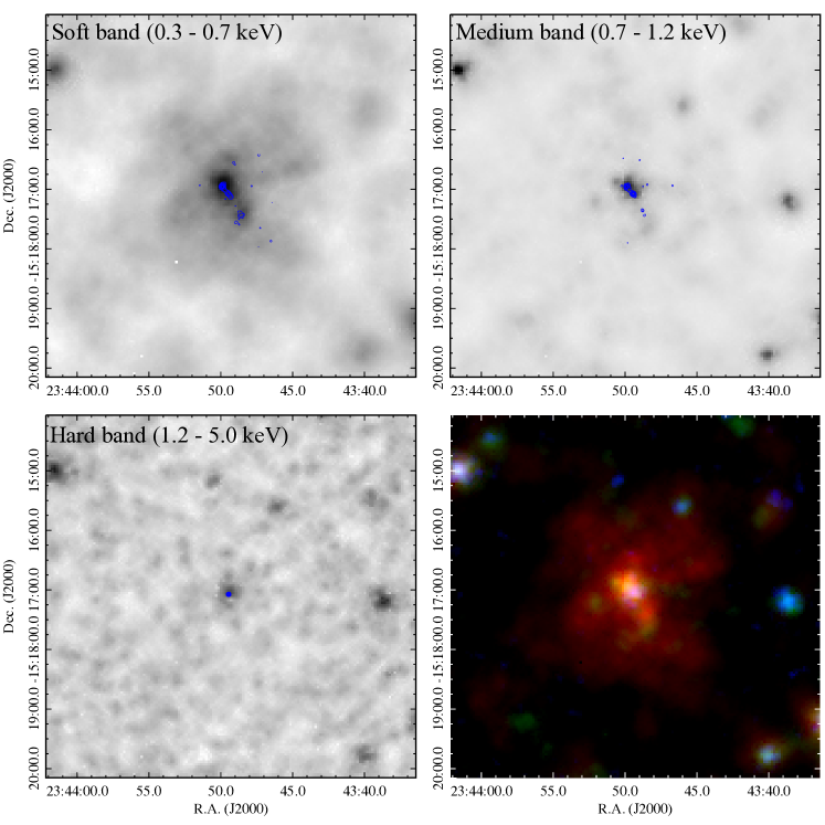
Figure 2: XMM-Newton EPIC images of the X-ray emission of R Aqr. Different panels show the soft (top left), medium (top right) and hard (bottom left) band images as well as a color-composite picture combining the three bands (bottom right). The blue contours correspond to the X-ray emission detected by Chandra on each band.

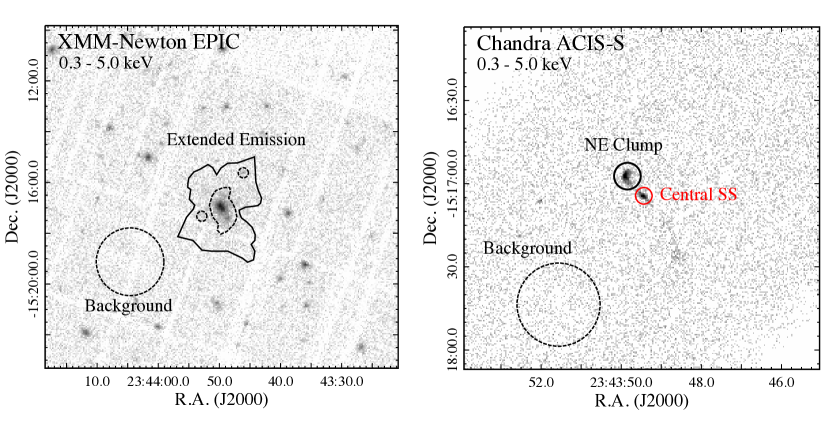
Figure 3: XMM-Newton EPIC (left) and Chandra ACIS-S (right) event file images produced for the 0.3–5.0 keV energy range. The spectra extraction regions are shown with solid line regions whilst the background extraction regions are shown with dashed-line circular apertures. The dashed-line apertures inside the extended emission were excised from the spectra extraction procedure. Note that unlike XMM-Newton, Chandra fully resolves the emission of the central SS from that of the NE clump.

To take advantage of the good quality of the XMM-Newton observations of R Aqr, we analyzed the EPIC data in two different ways. First, we started our analysis making use of the Extended Source Analysis Software (ESAS) package, currently included as part of the SAS. The data were processed following the cookbook for analysis of extended objects and diffuse background. The ESAS tasks apply restrictive event selection criteria, but their results leverage the presence of soft ($E<1.5$ keV) extended emission (see Snowden et al., 2004, 2008; Kuntz & Snowden, 2008).

After processing the data with the ESAS tasks, the final net exposure times of the MOS1, MOS2, and pn cameras are 33.8, 39.1, and 20.4 ks respectively. The processed files were used to create EPIC images in the 0.3–0.7 keV (soft), 0.7–1.2 keV (medium), and 1.2–5.0 keV (hard) energy bands. Individual pn, MOS1, and MOS2 images were extracted, corrected for exposure maps, and merged together. The soft, medium, and hard band images were adaptively smoothed using the ESAS task adapt requesting 30, 10, and 10 counts, respectively. The final images are presented in Figure 2 as well as a color-composite X-ray image combining the three bands.

To study the physical properties of the extended X-ray emission detected with XMM-Newton, we need to extract and model its spectrum. Since the ESAS event selection criteria are too restrictive for this purpose, we reprocessed the EPIC data this time using the epproc and emproc tasks. To remove periods of high background levels in the data, we produced light curves in the 10–12 keV energy range and excised time periods with count rates higher than 0.2 and 0.45 counts s^-1 for the MOS and pn cameras, respectively. After excising bad time intervals, the event files have net exposure times of 59.3, 60.0, and 35.8 ks for the MOS1, MOS2, and pn, respectively.

For comparison and discussion we also retrieved Chandra observations of R Aqr from the Chandra Data Archive. Several sets of Chandra observations R Aqr are available, but, given its X-ray variability, we choose to retrieve those observed at the same epoch of the XMM-Newton EPIC data, i.e., those corresponding to the Obs. ID. 5438 (PI: E. Kellogg) obtained on 2005 October 9 with a total exposure time of 66.7 ks. The data were obtained with the Advanced CCD Imaging Spectrometer (ACIS)-S in the VFAINT mode and R Aqr was registered on the back-illuminated CCD S3. The Chandra data were processed with the Chandra Interactive Analysis of Observations (CIAO, version 4.7.4; Fruscione et al., 2006).

3 Results

3.1 Extended X-ray emission

The XMM-Newton EPIC images produced with the ESAS tasks unambiguosly reveal the presence of extended X-ray emission associated with R Aqr. Figure 2 reveals the presence of X-ray emission up to 2.2^′ from the SS. In addition, Figure 2 shows that the bulk of the emission is emitted in the soft band. There is some extended emission detected in the medium band distributed in the inner $\sim$30^′′ very likely associated with the X-ray-bright clumps resolved in the Chandra data (see, e.g., Kellogg et al., 2007). The hard X-ray emission is only associated with the SS. This energy-dependent spatial distribution of the hot gas can be appreciated in the color-composite picture presented in the bottom-right panel of Figure 2.

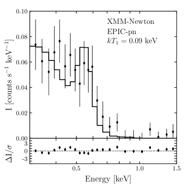
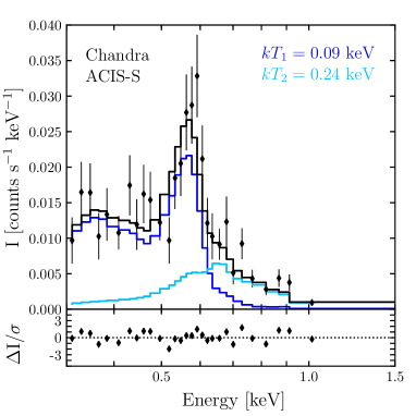
Figure 4: (left) Background-subtracted XMM-Newton EPIC-pn spectrum of the large-scale diffuse X-ray emission of R Aqr (left) and Chandra ACIS-S spectrum of its bright NE clump (right). The black dots correspond to the observed spectra whilst the black histograms represent the best fit models. The blue and cyan histograms in the right panel illustrate individual single-temperature components. (bottom) Residuals of the spectral fit.

Figure 2 also suggests that the soft X-ray emission has a bipolar morphology. A pair of conical structures open up to the northern and southern directions protruding from the central region. This situation is further illustrated in Figure 1-left that compares the XMM-Newton soft X-ray emission with narrow band images obtained with the VLT, making evident the match between the distributions of the X-ray-emitting gas and the large-scale optical nebular structures.

It is worth noting that the EPIC images does not resolve completely the emission in the central region of R Aqr, unlike the Chandra observations that trace in detail the hot gas associated with the bipolar jets of R Aqr (see Kellogg et al., 2007; Nichols et al., 2007). On the contrary, the Chandra data present negligible contribution of extended emission. This situation is illustrated in Figure 1, which shows composite optical and X-ray pictures using XMM-Newton EPIC (left) and Chandra ACIS-S (right) data. We confirm the different spatial-scales sampled by XMM-Newton and Chandra in Figure 3 by comparing the event files of the EPIC and ACIS-S cameras. The Chandra event files clearly resolve the contribution from the SS, the NE clump, and some extended emission towards the SW (see Fig. 3 right panel), which can only be hinted in the XMM-Newton event files. Contours of the soft, medium, and hard emission detected by Chandra and generated with the CIAO tasks aconvolve are also compared with the EPIC images in Figure 2.

3.2 Physical properties of the extended X-ray emission

XMM-Newton spectra were extracted from the EPIC pn camera, given its superior effective area compared with the MOS cameras. The spectrum of the extended emission was extracted from a region encompassing the soft X-ray emission. We excluded the central region which is dominated by the emission from the bipolar jet as well as a pair of background point-like sources (see Fig. 3). The background was extracted from a circular region with a radius of 80^′′ towards the SE from R Aqr (see Fig. 3 left panel). The spectrum and associated calibration matrices were created using the SAS tasks eveselect, rmfgen and arfgen. The resultant background-subtracted EPIC pn spectrum of the extended emission is presented in the left panel of Figure 4. The net count rate detected from the extended emission is 23.0$\pm$2.3 counts ks^-1.

For comparison we also extracted the spectrum from the brightest X-ray clump detected $\sim$10^′′ NE of R Aqr and resolved in the Chandra ACIS-S data (see Fig. 3 right panel). Its extraction region corresponds to a 4^′′-radius circular aperture, whilst the background was selected from a 15^′′-radius circular aperture towards the SW. The background-subtracted ACIS-S spectrum and calibration matrices were produced using the CIAO task specextract. The resultant background-subtracted Chandra ACIS-S spectrum of the NE clump is presented in the right panel of Figure 4. The NE clump has a net count rate of 6.9$\pm$0.3 counts ks^-1.

Both spectra are extremely soft and resemble those presented and analyzed by Kellogg et al. (2007). They exhibit the presence of the O vii triplet at 0.58 keV and prominent emission at energies below 0.5 keV. The latter includes the very likely emission from N vi at 0.43 keV and the Ly$\alpha$ C vi emission line at 0.37 keV. No significant emission is detected above 1.0 keV.

The spectral analysis was performed using XSPEC (Arnaud, 1996). We started by fitting single plasma emission models to the data, which we note it was enough for the EPIC spectrum, but according to Kellogg et al. (2007) the Chandra spectrum requires two-temperature apec optically-thin emission plasma models. The absorption was included with the tbabs model (Wilms et al., 2000) and all spectra were fit adopting solar abundances from Lodders (2003).

Table 1: Spectral fits of the diffuse X-ray emission in R Aqr.

Parameter		Extended Emission	NE Clump
		(EPIC pn)	(ACIS-S)
$\chi^{2}$		1.00	1.04
$N_{\mathrm{H}}$	[$10^{20}$ cm-2]	4.0 (fixed)	$8.0^{+11}_{-5.0}$
$kT_{1}$	[keV]	$0.09^{+0.01}_{-0.02}$.	$0.09^{+0.02}_{-0.03}$
$kT_{2}$	[keV]	…	$0.24^{+0.09}_{-0.05}$
$A_{1}$	[cm-5]	1.6$\times 10^{-4}$	4.3$\times 10^{-4}$
$A_{2}$	[cm-5]	…	1.2$\times 10^{-5}$
$f_{\mathrm{X}}$	[erg cm-2 s-1]	(4.4$\pm$1.5)$\times$10-14	(4.8$\pm$0.8)$\times$10-14
$F_{\mathrm{X}}$	[erg cm-2 s-1]	(7.7$\pm$2.6)$\times$10-14	(1.5$\pm$0.2)$\times$10-13
$L_{\mathrm{X}}^{\dagger}$	[erg s-1]	(1.4$\pm$0.5)$\times$1030	(2.7$\pm$0.4)$\times$1030

^†Adopting a distance of 385 pc.

We started by fitting the Chandra ACIS-S spectrum of the NE clump. The best fit model ($\chi^{2}$=1.04) resulted in plasma temperatures of $kT_{1}=0.09^{+0.02}_{-0.03}$ keV and $kT_{2}=0.24^{+0.09}_{-0.05}$ keV with normalization parameters of $A_{1}=4.3\times 10^{-4}$ cm^-5 and $A_{2}=1.2\times 10^{-5}$ cm^-5, respectively. The absorption column density of the model was $N_{\mathrm{H}}=(8^{+11}_{-5})\times 10^{20}$ cm^-2, consistent with the extinction estimate of $A_{\mathrm{V}}$=1–2 mag by Bujarrabal et al. (2021) towards R Aqr. The total observed flux in the 0.3–1.5 keV energy range is $f_{\mathrm{X}}=(4.8\pm 0.8)\times 10^{-14}$ erg cm^-2 s^-1 which corresponds to an intrinsic flux of $F_{\mathrm{X}}=(1.5\pm 0.2)\times 10^{-13}$ erg cm^-2 s^-1 and an X-ray luminosity of $L_{\mathrm{X}}=(2.7\pm 0.4)\times 10^{30}$ erg s^-1. We note that the softer component contributes to 85% of the total X-ray emission. Finally, we estimated an electron density of $n_{\mathrm{e}}\approx 40$ cm^-3 by adopting an averaged radius of 4^′′ for the NE clump. The model is compared with the observed Chandra ACIS-S spectrum in the right panel of Figure 4 and the details are listed in Table 1.

The spectral fit of the EPIC pn spectrum of the extended emission resulted in very similar properties as those of the NE clump. However, we note that we had to fix the absorption column density, because when left as a free parameter it converged to unphysical values. The $N_{\mathrm{H}}$ in the extended regions away from R Aqr should have less extinction than that of the central regions. The HEASARC $N_{\mathrm{H}}$ column density webpage estimates that in the vicinity of R Aqr this is $\sim 2\times 10^{20}$ cm^-2. Thus, we decided to fix the absorption column density to an intermediate value of $N_{\mathrm{H}}=4\times 10^{20}$ cm^-2. With this, the best fit model ($\chi^{2}=$1.00) has a dominant plasma temperature of $kT_{1}=0.09^{+0.01}_{-0.02}$ keV with normalization parameter of $A_{1}=1.6\times 10^{-4}$ cm^-5. The total observed flux in the 0.3–1.5 keV energy range is $f_{\mathrm{X}}=(4.4\pm 1.5)\times 10^{-14}$ erg cm^-2 s^-1 with an intrinsic flux of $F_{\mathrm{X}}=(7.7\pm 2.6)\times 10^{-14}$ erg cm^-2 s^-1, which corresponds to an X-ray luminosity of $L_{\mathrm{X}}=(1.4\pm 0.5)\times 10^{30}$ erg s^-1. The estimated electron density for the most extended emission of $n_{\mathrm{e}}\approx$0.5 cm^-3 adopting an averaged angular radius of 2^′. The best fit is compared to the EPIC pn spectrum in presented in the left panel of Figure 4 and the model details are also listed in Table 1.

We note that the observed surface brightness of the extended emission detected by XMM-Newton is a few times 10^-17 erg s^-1 cm^-2 arcsec^-2. This value is just at the detection limit of the ACIS-S instrument, thus explaining why it was not detected by Chandra.

Other models to the X-ray spectra were attempted. For example, we also tried plasma emission models with variable N abundance in order to fit the spectral feature at 0.43 keV, but such models did not improve the fit. Models adopting a power law distribution for the hardest component were also attempted. Such models resulted in good-quality fits ($\chi^{2}\approx 1$) too, suggesting that the physical origin of the second component can not be firmly established. Lastly, we note that other models taking into account non equlibrium thermal components or non equlibrium collisional model are difficult to constrain given the relative poor-quality of the spectra (see Kellogg et al., 2007).

4 Discussion and concluding remarks

The analysis of the XMM-Newton EPIC data with the ESAS tasks has revealed the presence of extended emission surrounding R Aqr in the soft (0.3–0.7 keV) X-ray band. The diffuse emission detected by EPIC seems to fill the gaps in between the nebular hourglass structures, extending to distances more than 2^′ towards the northern and southern regions from R Aqr (see, e.g., Fig. 1 left panel). The extension of the diffuse X-ray emission is consistent with the results discussed in Bujarrabal et al. (2021) where the orbital plane of the SS is seen almost edge-on and most of the dense gas is distributed in the equatorial plane, with lower density along the N-S directions that facilitates the expansion of the hot gas.

We found that the spectrum of the extended X-ray emission detected by XMM-Newton EPIC shares a very cool component with the spectrum of the NE clump associated with the S-shaped jet resolved by Chandra ACIS-S. This suggests that the jet is an ongoing structure that keeps feeding the extended, X-ray-emitting hot bubble. The cooling time of such hot but low density gas is long (see Kellogg et al., 2007) and, accordingly, no significant reduction of the temperature is observed between the jet and the most extended X-ray emission. The estimated $n_{\mathrm{e}}$ of the most extended gas is almost 80 times lower than that associated with the NE clump, implying a significantly smaller differential emission measure for the former. Thus, the gas expands adiabatically and cools down.

The nature of the harder component required in the spectral analysis of the X-ray-emitting jet is still unknown. This seems to be only spatially correlated with the collimated jet and it is not surprising that magnetic phenomena are responsible for the shaping (Burgarella et al., 1992; Melnikov, Stute, & Eislöffel, 2018). However, the search for non thermal emission in radio bands has been challenging (Hollis et al., 1985; Bujarrabal et al., 2018). Further analysis combining multi-epoch Chandra data will help shed light on the physical properties of the X-ray-emitting gas associated with jets (R. Montez Jr private communication).

The jet appears to be collimated, its S-shape is clearly indicative of precession. The precession angle is wide, $\approx 50^{\circ}$, as suggested by high-resolution Hubble Space Telescope images (Melnikov, Stute, & Eislöffel, 2018), and actually theoretical predictions state that opening angles larger than 40^∘ produce nebulae with pairs of inflated bubbles (Soker, 2004). We therefore suggest that blister-like structures at the tip of the precessing jet get disrupted and feed hot gas into the most extended hot bubble. The creation-destruction of the blister-like structures seems to be relatively fast given the evident expansion of the X-ray-emitting clumps resolved by Chandra (e.g., Kellogg et al., 2007). It is possible that the high pressure of the hot gas helped inflating the most extended lobe detected in optical wavelengths (see figure 2 of Liimets et al., 2018).

We also suggest that the continuous production and disruption of blister-like structures has created the bowl-like structures opening towards the northern and southern regions of R Aqr. Disk formation and jet launching has been studied through numerical simulations of binary systems in great detail (see, e.g., López-Cámara et al., 2020; Sheikhnezami & Fendt, 2018; Waters & Proga, 2018, and references therein), but the XMM-Newton EPIC observations analyzed here leverage the role of accretion process onto a compact object, a WD in this case, on the formation of hot bubbles and large-scale nebulae. This process might be similar, but in an evidently smaller scale, to the creation of hot bubbles produced by active galaxies hosting supermassive black holes (see, e.g., the case of Cen A; Król et al., 2020; Hardcastle et al., 2003, and references therein).

Several theoretical works have proposed the jet feedback mechanism (JFM) as the physics behind the production of inflated bipolar cavities in a wide variety of astronomical phenomena. The JFM successfully explains a diverse variety of objects regardless of differences of several orders of magnitude in size, energy injection, mass and timescales (Soker, 2016), from young stellar objects through planetary nebulae to galaxy clusters (e.g., Cliffe et al., 1995; Soker, 2002, 2004, 2016).

Deeper and higher-quality observations, as those provided by eROSITA and future missions such as Athena, might be able to disclose more extended X-ray emission with lower surface brightness of X-ray-emitting gas in R Aqr. A complete mapping of the diffuse X-ray hot bubble will help us study the feedback from SSs to create fast evolving nebulae around them.

The authos thank the anonymous referee for comments and suggestions that improved the analysis presented here. The authors are thankful to Tiina Liimets for providing the VLT narrow band images of R Aqr. They also acknowledge Rodolfo Montez Jr for fruitful discussion during the preparation of the manuscript. JAT acknowledges support by the Marcos Moshinsky Foundation (Mexico) and UNAM PAPIIT project IA101622 (Mexico). LS acknowledges support by UNAM PAPIIT project IN110122 (Mexico). MAG acknowledges support of grant PGC 2018-102184-B-I00 of the Ministerio de Educación, Innovación y Universidades cofunded with FEDER funds. GR-L acknowledges support from CONACyT grant 263373. YHC acknowledges the grant MOST 110-2112-M-001-020 from the Ministry of Science and Technology (Taiwan). Based on observations obtained with XMM-Newton, an ESA science mission with instruments and contributions directly funded by ESA Member States and NASA. This research has made use of data obtained from the Chandra Data Archive and software provided by the Chandra X-ray Center (CXC) in the application package CIAO. This work has made extensive use of the NASA’s Astrophysics Data System.

, CIAO (Fruscione et al., 2006)

References

- Arnaud (1996) Arnaud, K. A. 1996, Astronomical Data Analysis Software and Systems V, 101, 17
- Bujarrabal et al. (2021) Bujarrabal, V., Agúndez, M., Gómez-Garrido, M., et al. 2021, A&A, 651, A4. doi:10.1051/0004-6361/202141002
- Bujarrabal et al. (2018) Bujarrabal V., Alcolea J., Mikołajewska J., Castro-Carrizo A., Ramstedt S., 2018, A&A, 616, L3. doi:10.1051/0004-6361/201833633
- Burgarella et al. (1992) Burgarella, D., Vogel, M., & Paresce, F. 1992, A&A, 262, 83
- Cliffe et al. (1995) Cliffe, J. A., Frank, A., Livio, M., et al. 1995, ApJ, 447, L49. doi:10.1086/309559
- Favata et al. (2002) Favata, F., Fridlund, C. V. M., Micela, G., et al. 2002, A&A, 386, 204. doi:10.1051/0004-6361:20011387
- Fruscione et al. (2006) Fruscione, A., McDowell, J. C., Allen, G. E., et al. 2006, Proc. SPIE, 6270, 62701V. doi:10.1117/12.671760
- Gabriel et al. (2004) Gabriel, C., Denby, M., Fyfe, D. J., et al. 2004, Astronomical Data Analysis Software and Systems (ADASS) XIII, 314, 759
- Galloway & Sokoloski (2004) Galloway, D. K. & Sokoloski, J. L. 2004, ApJ, 613, L61. doi:10.1086/424925
- Gromadzki & Mikołajewska (2009) Gromadzki M., Mikołajewska J., 2009, A&A, 495, 931. doi:10.1051/0004-6361:200810052
- Hardcastle et al. (2003) Hardcastle, M. J., Worrall, D. M., Kraft, R. P., et al. 2003, ApJ, 593, 169. doi:10.1086/376519
- Hollis, Pedelty, & Lyon (1997) Hollis J. M., Pedelty J. A., Lyon R. G., 1997, ApJL, 482, L85. doi:10.1086/310687
- Hollis et al. (1985) Hollis, J. M., Kafatos, M., Michalitsianos, A. G., et al. 1985, ApJ, 289, 765. doi:10.1086/162940
- Hunsch et al. (1998) Hunsch, M., Schmitt, J. H. M. M., Schroder, K.-P., et al. 1998, A&A, 330, 225
- Jura & Helfand (1984) Jura, M. & Helfand, D. J. 1984, ApJ, 287, 785. doi:10.1086/162737
- Kafatos & Michalitsianos (1982) Kafatos M., Michalitsianos A. G., 1982, Natur, 298, 540. doi:10.1038/298540a0
- Kellogg et al. (2009) Kellogg, E. M., Nichols, J., & Anderson, C. 2009, \aas, meeting #213, Vol. 41, p. 279
- Kellogg et al. (2007) Kellogg, E., Anderson, C., Korreck, K., et al. 2007, ApJ, 664, 1079. doi:10.1086/518877
- Kellogg et al. (2001) Kellogg, E., Pedelty, J. A., & Lyon, R. G. 2001, ApJ, 563, L151. doi:10.1086/338594
- Król et al. (2020) Król, D. Ł., Marchenko, V., Ostrowski, M., et al. 2020, ApJ, 903, 107. doi:10.3847/1538-4357/abb8d8
- Kuntz & Snowden (2008) Kuntz, K. D. & Snowden, S. L. 2008, A&A, 478, 575. doi:10.1051/0004-6361:20077912
- Liimets et al. (2018) Liimets T., Corradi R. L. M., Jones D., Verro K., Santander-García M., Kolka I., Sidonio M., et al., 2018, A&A, 612, A118. doi:10.1051/0004-6361/201732073
- Lodders (2003) Lodders, K. 2003, ApJ, 591, 1220. doi:10.1086/375492
- López-Cámara et al. (2020) López-Cámara, D., Moreno Méndez, E., & De Colle, F. 2020, MNRAS, 497, 2057. doi:10.1093/mnras/staa1983
- Mayer et al. (2013) Mayer, A., Jorissen, A., Kerschbaum, F., et al. 2013, A&A, 549, A69. doi:10.1051/0004-6361/201219259
- Melnikov, Stute, & Eislöffel (2018) Melnikov S., Stute M., Eislöffel J., 2018, A&A, 612, A77. doi:10.1051/0004-6361/201731749
- Michalitsianos, Kafatos, & Hobbs (1980) Michalitsianos A. G., Kafatos M., Hobbs R. W., 1980, ApJ, 237, 506. doi:10.1086/157895
- Michalitsianos et al. (1988) Michalitsianos A. G., Oliversen R. J., Hollis J. M., Kafatos M., Crull H. E., Miller R. J., 1988, AJ, 95, 1478. doi:10.1086/114743
- Montez et al. (2021) Montez, R., Luna, G. J. M., Mukai, K., et al. 2021, arXiv:2110.04315
- Nichols et al. (2007) Nichols J. S., DePasquale J., Kellogg E., Anderson C. S., Sokoloski J., Pedelty J., 2007, ApJ, 660, 651. doi:10.1086/512138
- Paresce & Hack (1994) Paresce, F. & Hack, W. 1994, A&A, 287, 154
- Rodríguez-Kamenetzky et al. (2019) Rodríguez-Kamenetzky, A., Carrasco-González, C., González-Martín, O., et al. 2019, MNRAS, 482, 4687. doi:10.1093/mnras/sty3055
- Sahai et al. (2003) Sahai, R., Kastner, J. H., Frank, A., et al. 2003, ApJ, 599, L87. doi:10.1086/381316
- Schmid et al. (2017) Schmid H. M., Bazzon A., Milli J., Roelfsema R., Engler N., Mouillet D., Lagadec E., et al., 2017, A&A, 602, A53. doi:10.1051/0004-6361/201629416
- Sheikhnezami & Fendt (2018) Sheikhnezami, S. & Fendt, C. 2018, ApJ, 861, 11. doi:10.3847/1538-4357/aac5dc
- Snowden et al. (2008) Snowden, S. L., Mushotzky, R. F., Kuntz, K. D., et al. 2008, A&A, 478, 615. doi:10.1051/0004-6361:20077930
- Snowden et al. (2004) Snowden, S. L., Collier, M. R., & Kuntz, K. D. 2004, ApJ, 610, 1182. doi:10.1086/421841
- Soker (2016) Soker, N. 2016, New Astro. Rev., 75, 1. doi:10.1016/j.newar.2016.08.002
- Soker (2004) Soker, N. 2004, A&A, 414, 943. doi:10.1051/0004-6361:20034120
- Soker (2002) Soker, N. 2002, ApJ, 568, 726. doi:10.1086/339065
- Solf & Ulrich (1985) Solf J., Ulrich H., 1985, A&A, 148, 274
- Stute et al. (2013) Stute, M., Luna, G. J. M., Pillitteri, I. F., et al. 2013, A&A, 554, A56. doi:10.1051/0004-6361/201218998
- Stute & Sahai (2009) Stute, M. & Sahai, R. 2009, A&A, 498, 209. doi:10.1051/0004-6361/200811176
- Toalá et al. (2020) Toalá, J. A., Guerrero, M. A., Santamaría, E., et al. 2020, MNRAS, 495, 4372. doi:10.1093/mnras/staa1502
- Viotti et al. (1987) Viotti R., Piro L., Friedjung M., Cassatella A., 1987, ApJL, 319, L7. doi:10.1086/184945
- Wallerstein & Greenstein (1980) Wallerstein G., Greenstein J. L., 1980, PASP, 92, 275. doi:10.1086/130663
- Waters & Proga (2018) Waters, T. & Proga, D. 2018, MNRAS, 481, 2628. doi:10.1093/mnras/sty2398
- Wilms et al. (2000) Wilms, J., Allen, A., & McCray, R. 2000, ApJ, 542, 914. doi:10.1086/317016