Actuator Scheduling for Linear Systems: A Convex Relaxation Approach

Abstract

In this letter, we investigate the problem of actuator scheduling for networked control systems. Given a stochastic linear system with a number of actuators, we consider the case that one actuator is activated at each time. This problem is combinatorial in nature and NP hard to solve. We propose a convex relaxation to the actuator scheduling problem, and use its solution as a reference to design an algorithm for solving the original scheduling problem. Using dynamic programming arguments, we provide a suboptimality bound of our proposed algorithm. Furthermore, we show that our framework can be extended to incorporate multiple actuator scheduling at each time and actuation costs. A simulation example is provided, which shows that our proposed method outperforms a random selection approach and a greedy selection approach.

I Introduction

In recent years, networked control systems (NCSs) have gained much interest in the controls community due to the advancements in communication architecture, computer technology, and network infrastructure that enable efficient distributed sensing, estimation, and control [1, 2, 3]. Potential applications include smart buildings [4], industrial and environmental control [5]. Due to potential constraints on the communication and computation resources of NCSs, sensor scheduling and actuator scheduling are two important and challenging problems, and efficient algorithms are sought for solving them.

The majority of the existing work focuses on sensor scheduling problems and their variants. Several approaches (e.g., stochastic selection [6], search tree pruning [7], greedy selection [8], semidefinite programming based trajectory tracking [9]) have been proposed to solve such problems. In contrast, the actuator scheduling problem has received much lesser attention. While sensor scheduling problems focus on minimizing (a function of) the estimation error, the actuator scheduling directly affects the controllability and stability of the system as well as the control performance. Therefore, a significant portion of the work on actuator scheduling focuses on studying the effects of actuator scheduling on the controllability and stability of the systems, e.g., [10, 11, 12, 13, 14] and others. It is shown in [10, 11, 12] that several classes of energy related metrics associated with the controllability Gramian have a structural property (modularity) that allows for an approximation guarantee by using a simple greedy heuristic. These problems are further investigated in [13], where a framework of sparse actuator schedule design was developed that guarantees performance bounds for a class of controllability metrics. Except [14], these works assume a time invariant scheduling problem, which is likely to be suboptimal and may impose restrictions on controllability for large systems. In [14] the authors use a round robin scheme for selecting the actuators and show that local stability is attained if the switching between the actuators is fast enough. The efficacy of a time-varying scheduling over a time-invariant one for interconnected systems is also demonstrated in [15]. However, how to find the optimal time-varying schedule still remains unanswered.

The efficacy of the abovementioned controllers on a system with different performance criteria (e.g., a quadratic cost function) is unknown and likely to be suboptimal since these works solely focus on the controllability and stability aspect of the system. In contrast to those works, a few existing works [16, 17, 18] consider a linear-quadratic optimal control problem for actuator scheduling. However, the focus on these works is to decide whether to activate the one single actuator available at each time or not.

Motivated by the above, in this letter we study the actuator scheduling problem for a finite horizon linear-quadratic control system with a number of actuators. We consider the case that a nonempty subset of the actuators is active at each time. The performance of the actuator schedule is measured by a finite horizon quadratic cost function of the system state and control plus the cost of using each actuator (representing e.g., energy consumption). This problem is combinatorial in nature and is NP-hard in general. Due to space limitations, we first restrict ourselves to the case that only one actuator is activated at each time and that all actuators have equal actuation costs. We then provide discussions and simulation results on the general cases that multiple actuators are activated at each time and that the actuators have different actuation costs.

The main contributions of this letter are the following: (i) We propose a convex relaxation to the actuator scheduling problem, and use its solution as a ‘reference’ to design an algorithm for solving the original NP-hard scheduling problem. (ii) We provide a suboptimality bound for the proposed algorithm. (iii) We further show that our results can be extended to the cases with multiple actuator scheduling and actuation costs.

The outline of this letter is as follows: In Section II, we formulate the actuator scheduling problem, which is solved in Section III. In Section IV, we provide discussions on multiple actuator scheduling and actuation costs. Simulation results are provided in Section V. Section VI concludes this letter.

Notation: We denote the set of real numbers and positive real numbers by $\mathbb{R}$ and $\mathbb{R}_{+}$, respectively. The set of $n$ dimensional vectors over $\mathbb{R}$ is denoted by $\mathbb{R}^{n}$ and the set of real $n\times m$ matrices is denoted by $\mathbb{R}^{n\times m}$. The identity matrix is denoted by $I$. For a given matrix $A$, its transpose and inverse (if exists) are denoted by $A^{\top}$ and $A^{-1}$, respectively. For a symmetric matrix $P$, we denote $P\succ 0$ ($P\succeq 0$) if it is positive definite (positive semidefinite). The trace of a square matrix $A$ is denoted by ${\rm tr}(A)$. The Frobenious norm of a matrix $A$ is denoted by $\|A\|_{F}$. We use $\mathbb{E}[x]$ to denote the expectation of a random variable $x$.

II Problem Formulation

We consider a system with $N$ actuators of the form

$$x_{t+1}=A_{t}x_{t}+\textstyle\sum_{j=1}^{N}\gamma_{t}(j)B_{t}(j)u_{t}(j)+w_{t},$$ (1)

where $A_{t}\in\mathbb{R}^{n\times n}$, $B_{t}(j)\in\mathbb{R}^{n\times m_{j}}$, $x_{t}\in\mathbb{R}^{n}$ the state, $u_{t}(j)\in\mathbb{R}^{m_{j}}$ the input from the $j$-th actuator, and $w_{t}\in\mathbb{R}^{n}$ an independent sequence of Gaussian random variables with $w_{t}\sim\mathcal{N}(0,W_{t})$. The initial state is $x_{0}\sim\mathcal{N}(0,W_{-1})$ and it is independent of $w_{t}$ for all $t$. The matrix $B_{t}(j)$ describes how the control input, $u_{t}(j)$, of the $j$-th actuator enters the system at the time $t$. The parameters $\gamma_{t}(j)$ are binary-valued such that $\gamma_{t}(j)=1$ if the $j$-th actuator is activated at the time $t$ and $\gamma_{t}(j)=0$ otherwise.

We consider the actuator scheduling problem that at each time only $N_{t}(1\leq N_{t}\leq N)$ out of the $N$ actuators are used to control the system (1) at time $t$. In this case, $\gamma_{t}(j)=1$ for $N_{t}$ out of all $N$ actuators at the time $t$.

Consider a standard finite horizon quadratic cost function

$$J_{1}=\mathbb{E}\Big{[} \textstyle\sum_{t=0}^{T-1}\Big{(}x_{t}^{\top}Q_{t}x_{t}+\sum_{j=1}^{N}\gamma_{t}(j){u_{t}(j)}\!^{\top}R_{t}(j)u_{t}(j)\Big{)}$$

$$+x_{T}^{\top}Q_{T}x_{T}\Big{]},$$ (2)

where $Q_{t},R_{t}(j)\succ 0$ for all $t$. In addition, consider also the actuation cost function $J_{2}=\sum_{t=0}^{T-1}\sum_{j=1}^{N}\gamma_{t}(j)c_{t}(j),$ where $c_{t}(j)\in\mathbb{R}_{+}$ is the cost of using actuator $j$ at time $t$. Note that $c_{t}(i)$ and $c_{t}(j)$ are in general different for $i\neq j$ and $i,j\in\mathsf{N}\triangleq\{1,2,\ldots,N\}$, which can be due to the fact that different actuators may have different energy consumption or resource usage. The objective of the actuator scheduling problem is then to find an actuator schedule that minimizes the joint control-actuation cost $J=J_{1}+J_{2}$.

Due to space limitations, in the sequel we will restrict ourselves to the case that $N_{t}=1$ and $c_{t}(j)=c_{t}$ for all $j$. In other words, we consider the case that exactly one out of the $N$ actuators is used at each time and that each actuator has the same actuation cost. The assumption $c_{t}(j)=c_{t}$ leads to $J_{2}$ being independent of the actuator schedule and therefore, minimizing $J$ is equivalent to minimizing $J_{1}$. The discussions on the cases with multiple actuators and actuation costs will be provided afterwards in Section IV.

Since only one actuator is used at each time and the actuation cost is independent of the chosen actuator, system (1) can now be rewritten as

$$x_{t+1}=A_{t}x_{t}+B_{t}(j)u_{t}(j)+w_{t},\ j\in\mathsf{N},$$ (3)

and the associated cost function becomes

$$\textstyle J=\mathbb{E}\Big{[}x_{T}^{\top}Q_{T}x_{T}+\sum_{t=0}^{T-1}\Big{(}x_{t}^{\top}Q_{t}x_{t}+{u_{t}(j)}^{\top}R_{t}(j)u_{t}(j)\Big{)}\Big{]}.$$ (4)

Let $\sigma:[0,T-1]\to\mathsf{N}$ be an actuator schedule function such that $\sigma(t)=j$ denotes that the $j$-th actuator is used at time $t$ to control the system (3). The objective is to find an actuator schedule $\sigma$ that minimizes the cost function (4). We assume that perfect state measurement is available. The information available at the controller at time $t$ is denoted by $\mathcal{I}_{t}$, with $\mathcal{I}_{t}=\mathcal{I}_{t-1}\bigcup\{x_{t}\}$ for all $t\geq 1$ and $\mathcal{I}_{0}=\{x_{0}\}$. Therefore, the (optimal) controller associated with the $j$-th actuator is

$$u_{t}(j)=L_{t}(j)\mathbb{E}[x_{t}\mid\mathcal{I}_{t}]=L_{t}(j)x_{t},\quad j\in\mathsf{N},$$ (5)

where the gain matrix $L_{t}(j)$ is given by

$$L_{t}(j)=-S_{t}(j)^{-1}{B_{t}(j)}^{\top}K_{t+1}(\sigma)A_{t},$$ (6)

and the matrices $K_{t}(\sigma),S_{t}(j)\succ 0$ are given recursively by

$$S_{t}(j):={B_{t}(j)}^{\top}K_{t+1}(\sigma)B_{t}(j)+R_{t}(j)$$ (7)

$$K_{t}(\sigma)=Q_{t}+A_{t}^{\top}K_{t+1}(\sigma)A_{t}-$$

$$~{}~{}~{}A_{t}^{\top}K_{t+1}(\sigma)B_{t}(\sigma(t))S_{t}(\sigma(t))^{-1}{B_{t}(\sigma(t))}^{\top}\!K_{t+1}(\sigma)A_{t}$$

$$K_{T}(\sigma):=K_{T}=Q_{T}.$$ (8)

Note that, until now, we have not yet not fixed the schedule $\sigma(t)$ at time $t$, and $j$ denotes the $j$-th actuator. Notice that, for any $t\leq T-1$, the matrix $K_{t}(\sigma)$ depends on the actuator schedule for the interval $[t,T-1]$. Therefore, the matrix $S_{t}(j)$ defined in (7) depends on the actuator schedule for the interval $[t+1,T-1]$, since it depends on $K_{t+1}(\sigma)$. Thus, the optimal gain $L_{t}(j)$ associated with the $j$-th actuator depends on the future schedule for the time interval $[t+1,T-1]$. From the LQG theory [19], the cost $J$ for a given schedule $\sigma$ is equal to $\sum_{t=0}^{T}{\rm tr}(K_{t}(\sigma)W_{t-1})$.

Before proceeding, to maintain brevity in the subsequent analysis, we define two matrix valued functions:

$$g_{t}(j,M):=M$$

$$~{}~{}~{}-M{B_{t}(j)}\big{(}{B_{t}(j)}\!^{\top}M{B_{t}(j)}+R_{t}(j)\big{)}^{-1}{B_{t}(j)}\!^{\top}M,$$ (9a)

$$h_{t}(M):=A_{t}^{\top}MA_{t}+Q_{t}.$$ (9b)

By substituting (9) into (8), we obtain that

$$K_{t\mid t+1}(\sigma):=g_{t}({\sigma(t)},K_{t+1}(\sigma)),$$ (10a)

$$K_{t}(\sigma)=h_{t}(K_{t\mid t+1}(\sigma)),\quad K_{T}=Q_{T}.$$ (10b)

In what follows, we will supress $\sigma(t)=\sigma$ to maintain notation brevity. The optimal actuator scheduling problem that we consider is then formulated as follows.

Problem 1 (Actuator Scheduling Problem)

Given system (3) and $N$ actuators, find a schedule $\sigma:[0,T-1]\to\mathsf{N}$ that solves the following optimization problem:

$$\min\ {\textstyle\sum_{t=0}^{T}{\rm tr}(K_{t}(\sigma)W_{t-1})}$$

subject to $$K_{t\mid t+1}(\sigma)=g_{t}({\sigma},K_{t+1}(\sigma)),\ {Q_{T}\succ 0,}$$

$$K_{t}(\sigma)=h_{t}(K_{t\mid t+1}(\sigma)),\ K_{T}=Q_{T}$$

with the variables $\sigma,K_{t},K_{t\mid t+1}.$

Problem 1 is combinatorial in nature and NP-hard in general [20]. We now propose an efficient solution to Problem 1 using a convex relaxation.

III Actuator Scheduling with Suboptimality Guarantees

In this section, we solve Problem 1 and provide a suboptimal solution that is computationally inexpensive. We will propose a convex relaxation to the problem (see Problem 3) and will use the solution of the relaxed problem as a ‘reference’ to find a solution to Problem 1. In Section III-A we will propose a tracking algorithm that finds a solution which is ‘close’ to the reference solution found from solving the relaxed convex optimization problem. The suboptimality bound of the proposed algorithm is discussed using dynamic programming type arguments in Section III-B.

Before proceeding, we first reformulate Problem 1 into a form that is easier for the analysis afterwards. According to (9b) and (10b), we have $K_{t}(\sigma)=A_{t}^{\top}K_{t|t+1}(\sigma)A_{t}+Q_{t}$, $t=0,1,\ldots,T-1$ and $K_{T}=Q_{T}$. Subsequently, we obtain

$$\textstyle\sum_{t=0}^{T}{\rm tr}(K_{t}(\sigma)W_{t-1})=\sum_{t=0}^{T-1}{\rm tr}(K_{t|t+1}(\sigma)\bar{W}_{t-1})+r,$$ (11)

where $r=\sum_{t=0}^{T}{\rm tr}(Q_{t}W_{t-1})$ and $\bar{W}_{t-1}=A_{t}W_{t-1}A_{t}^{\top}$. Note that $r$ is independent of $\sigma,K_{t}(\sigma)$ and $K_{t\mid t+1}(\sigma).$

Next, we define two matrices $P_{t}$ and $P_{t|t+1}$ as follows

$$\textstyle P_{t}(\sigma):=K_{t}^{-1}(\sigma),\quad P_{t\mid t+1}(\sigma):=K^{-1}_{t\mid t+1}(\sigma).$$

According to Woodbury matrix equality, we have

$$P_{t\mid t+1}(\sigma)=P_{t+1}(\sigma)+B_{t}({\sigma})R_{t}^{-1}({\sigma})B_{t}^{\top}({\sigma}).$$ (12)

Using (11) and the new variables $P_{t\mid t+1}(\sigma)$, $P_{t}(\sigma)$, Problem 1 can be rewritten as Problem 2.

Problem 2

Given system (3) with $N$ actuators, find a schedule $\sigma:[0,T-1]\to\mathsf{N}$ that solves the following:

$$\min\ {\textstyle\sum_{t=0}^{T-1}{\rm tr}(K_{t|t+1}(\sigma)\bar{W}_{t-1})}$$

subject to $$K_{t\mid t+1}(\sigma)=P^{-1}_{t\mid t+1}(\sigma),\ {Q_{T}\succ 0,}$$

$$P_{t\mid t+1}(\sigma)=P_{t+1}(\sigma)+B_{t}({\sigma})R_{t}^{-1}({\sigma})B_{t}^{\top}({\sigma}),$$

$${P^{-1}_{t}(\sigma)=h_{t}(K_{t\mid t+1}(\sigma))},\ P_{T}=Q_{T}^{-1}$$

with variables $\sigma,K_{t},K_{t\mid t+1},P_{t},P_{t\mid t+1}.$

Note that, although the constraints in Problem 1 and Problem 2 appear differently, one can in fact verify that these two problems are equivalent.

Let us denote $V_{t}(\sigma):=B_{t}({\sigma})R_{t}^{-1}({\sigma})B_{t}^{\top}({\sigma})$ and the set $\mathsf{V}_{t}:=\{{B_{t}(j)}{R_{t}(j)}^{-1}{B_{t}(j)}^{\top}~{}:~{}j\in\mathsf{N}\}$. Therefore, we may rewrite the constraints in Problem 2 to be $K_{t\mid t+1}=P^{-1}_{t\mid t+1},\ P_{t\mid t+1}=P_{t+1}+V_{t},\ V_{t}\in\mathsf{V}_{t},\ P_{t}=\big{(}h_{t}(K_{t\mid t+1})\big{)}^{-1},$ and $P_{T}=Q_{T}^{-1}.$ We have suppressed the arguments $\sigma$ in the variables to maintain notational brevity. We can further relax the constraints in Problem 2 to their equivalent matrix inequality $K_{t\mid t+1}\succeq P^{-1}_{t\mid t+1}$, and $P_{t}\preceq(h_{t}(K_{t\mid t+1}))^{-1}$. Using Schur complement, one may write $K_{t\mid t+1}\succeq P^{-1}_{t\mid t+1}$ as the Linear matrix inequality $\begin{bmatrix}K_{t\mid t+1}&I\\ I&P_{t\mid t+1}\end{bmatrix}$ $\succeq 0$. Similarly, using the definition of $h_{t}(\cdot)$ from (9b), the Woodbury matrix inverse identity, and Schur complement, we obtain the following problem from Problem 2.

Problem 3

Given $\mathsf{V}_{t}:=\{{B_{t}(j)}{R_{t}(j)}^{-1}{B_{t}(j)}^{\top}~{}:~{}j\in\mathsf{N}\}\subset\mathbb{R}^{n\times n}$, solve the following optimization problem

$$\min\ {\textstyle\sum_{t=0}^{T-1}{\rm tr}(K_{t|t+1}\bar{W}_{t-1})}$$

subject to $$P_{t\mid t+1}=P_{t+1}+V_{t},\ V_{t}\in\mathsf{V}_{t},\ P_{T}=Q_{T}^{-1},$$

$$\begin{bmatrix}K_{t\mid t+1}&I\\ I&P_{t\mid t+1}\end{bmatrix}\succeq 0,\ {Q_{T}\succ 0,}$$

$$\begin{bmatrix}Q_{t}^{-1}-P_{t}&Q_{t}^{-1}A_{t}^{\top}\\ A_{t}Q_{t}^{-1}&P_{t\mid t+1}+A_{t}Q_{t}^{-1}A_{t}^{\top}\end{bmatrix}\succeq 0$$

with variables $K_{t\mid t+1},P_{t\mid t+1},P_{t}$, and $V_{t}$.

Notice that the constraint $V_{t}\in\mathsf{V}_{t}$ is sufficient to enforce the scheduling constraint $\sigma:[0,T-1]\to\mathsf{N}$.

While Problem 3 is a relaxation of Problem 2, we now show a key result that an optimal solution to Problem 3 is also an optimal solution to Problem 2.

Theorem 1

An optimal solution of the relaxed problem (Problem 3) is also an optimal solution of the original problem (Problem 2), and vice-versa.

Proof:

The proof of this theorem is along the lines of [9, Theorem 1]. First, note that, due to the relaxations, any feasible solution of Problem 2 is a feasible solution for Problem 3, and hence the optimal solution of Problem 2 is a feasible solution for Problem 3. The theorem is proved once we show that for every feasible solution of Problem 3 there exists a feasible solution for Problem 2 that produces the same, if not a smaller, objective value.

In order to show that, let the tuple $\{K_{t\mid t+1},P_{t\mid t+1},P_{t}\}$ denote a feasible solution of Problem 3. Let us construct a new tuple $\{\bar{K}_{t\mid t+1},\bar{P}_{t\mid t+1},\bar{P}_{t}\}$ as follows

$$\bar{P}_{t\mid t+1}=\bar{P}_{t+1}+\bar{V}_{t},\quad\bar{P}_{t}=\big{(}h_{t}(\bar{K}_{t\mid t+1})\big{)}^{-1}$$ (13)

$$\bar{V}_{t}={P}_{t\mid t+1}-{P}_{t+1},\quad\bar{K}_{t\mid t+1}=\bar{P}^{-1}_{t\mid t+1},\quad\bar{P}_{T}=P_{T}.$$

We will now show that $\bar{P}_{t\mid t+1}\succeq{P}_{t\mid t+1}$, $\bar{K}_{t\mid t+1}\preceq K_{t\mid t+1}$ and $\bar{P}_{t+1}\succeq P_{t+1}$ for all $t$. We start with $t=T$, it follows from $\bar{P}_{T}=P_{T}$ that $\bar{P}_{T}\succeq P_{T}$. Since $\bar{P}_{t\mid t+1}=\bar{P}_{t+1}+\bar{V}_{t}$ and $\bar{V}_{t}={P}_{t\mid t+1}-{P}_{t+1}$, it follows that $\bar{P}_{T-1\mid T}-{P}_{T-1\mid T}=\bar{P}_{T}-{P}_{T}$. Since $\bar{P}_{T}\succeq P_{T}$, this implies that $\bar{P}_{T-1\mid T}\succeq{P}_{T-1\mid T}.$ Note that $\bar{P}_{T-1\mid T}\succeq{P}_{T-1\mid T}\succ 0$, it then follows that $\bar{P}_{T-1\mid T}^{-1}\preceq{P}_{T-1\mid T}^{-1}$. Now, recall that $K_{t\mid t+1}\succeq P^{-1}_{t\mid t+1}$, and that $\bar{K}_{t\mid t+1}=\bar{P}^{-1}_{t\mid t+1}$ in (13). It then follows that

$$\bar{K}_{T-1\mid T}=\bar{P}^{-1}_{T-1\mid T}\preceq{P}_{T-1\mid T}^{-1}\preceq{K}_{T-1\mid T},$$

that is $\bar{K}_{T-1\mid T}\preceq{K}_{T-1\mid T}.$ Next, recall that

$$\bar{P}_{t}^{-1}=h_{t}(\bar{K}_{t\mid t+1}):=A_{t}^{\top}\bar{K}_{t\mid t+1}A_{t}+Q_{t},$$

$${P}_{t}^{-1}=h_{t}({K}_{t\mid t+1}):=A_{t}^{\top}{K}_{t\mid t+1}A_{t}+Q_{t}.$$

It then follows from $\bar{K}_{T-1\mid T}\preceq{K}_{T-1\mid T}$ that $\bar{P}_{T-1}^{-1}\preceq P_{T-1}^{-1}$. This implies that $\bar{P}_{T-1}\succeq P_{T-1}.$ By induction, the same procedure applies for all $t=T-1,T-2,\ldots,0$. Thus, $\bar{P}_{t\mid t+1}\succeq{P}_{t\mid t+1}$, $\bar{K}_{t\mid t+1}\preceq K_{t\mid t+1}$ and $\bar{P}_{t+1}\succeq P_{t+1}$ for all $t$.

Next, let $K_{t\mid t+1},P_{t\mid t+1},P_{t}$, and $V_{t}$ be solutions of Problem 3. Then $K_{t\mid t+1},P_{t\mid t+1},P_{t}$, and $V_{t}$ satisfy the constraints of Problem 3, in particular, $P_{t\mid t+1}=P_{t+1}+V_{t},\ V_{t}\in\mathsf{V}_{t}$. This implies that $V_{t}=P_{t\mid t+1}-P_{t+1},\ V_{t}\in\mathsf{V}_{t}.$ Now, recall that in (13) we have chosen $\bar{V}_{t}={P}_{t\mid t+1}-{P}_{t+1}$. It then follows from $\bar{V}_{t}={P}_{t\mid t+1}-{P}_{t+1}$ and $V_{t}=P_{t\mid t+1}-P_{t+1},\ V_{t}\in\mathsf{V}_{t}$ that $\bar{V}_{t}\in{\sf V}_{t}$.

Now, since the tuple $\{\bar{K}_{t\mid t+1},\bar{P}_{t\mid t+1},\bar{P}_{t}\}$ satisfies all the constraints of Problem 2, this implies that it is a feasible solution of Problem 2. Next, note that $\bar{K}_{t\mid t+1}\preceq{K}_{t\mid t+1}$ for all $t$, this then implies that $\sum_{t=0}^{T-1}\mathrm{tr}(\bar{K}_{t\mid t+1}\bar{W}_{t-1})\preceq\sum_{t=0}^{T-1}\mathrm{tr}(K_{t\mid t+1}\bar{W}_{t-1})$. Therefore, for any feasible solution of Problem 3 we can construct a feasible solution for Problem 2 that produces the same, if not less, cost. This completes the proof. ∎

Remark 2

Theorem 1 shows that the LMI-based relaxations introduced in Problem 3 do not affect the optimality, since an optimal solution to the relaxed problem is also optimal for the original problem. This is a key advantage of this approach, as the LMI-based relaxations retain the optimality. Moreover, since Problem 3 is a mixed integer semidefinite program, one may attempt to directly solve it using available numerical techniques [21].

Next, note that Problem 3 is convex if $\mathsf{V}_{t}$ is a convex set for all $t$. When $\mathsf{V}_{t}$ is not convex, one could take the convex hull of the set $\mathsf{V}_{t}$ to make Problem 3 convex. In our case, since $\mathsf{V}_{t}$ is a collection of $N$ matrices $\{V_{t}(1),\ldots,V_{t}(N)\}$ where $V_{t}(j)={B_{t}(j)}{R_{t}(j)}^{-1}{B_{t}(j)}^{\top}$ for all $t$, we replace the constraint $V_{t}\in\mathsf{V}_{t}$ with the constraints $V_{t}=\sum_{i=1}^{N}\theta^{i}_{t}V_{t}(i)$, $\theta^{i}_{t}\in[0,1]$ and $\sum_{i=1}^{N}\theta^{i}_{t}=1$. In this case, Problem 3 can be further simplified to Problem 4.

Problem 4

$$\min\ {\textstyle\sum_{t=0}^{T-1}{\rm tr}(K_{t|t+1}\bar{W}_{t-1})}$$

subject to $$P_{t\mid t+1}=P_{t+1}+\textstyle\sum_{i=1}^{N}\theta^{i}_{t}V_{t}(i),\ P_{T}=Q_{T}^{-1},$$

$$\textstyle\sum_{i=1}^{N}\theta^{i}_{t}=1,0\leq\theta^{i}_{t}\leq 1,\begin{bmatrix}K_{t\mid t+1}&I\\ I&P_{t\mid t+1}\end{bmatrix}\succeq 0,$$

$$\begin{bmatrix}Q_{t}^{-1}-P_{t}&Q_{t}^{-1}A_{t}^{\top}\\ A_{t}Q_{t}^{-1}&P_{t\mid t+1}+A_{t}Q_{t}^{-1}A_{t}^{\top}\end{bmatrix}\succeq 0,{Q_{T}\succ 0}$$

with variables $\theta_{t}^{i},K_{t\mid t+1},P_{t\mid t+1},P_{t}$.

At this point we have a convex optimization problem (semidefinite program) in Problem 4 which is much easier to solve compared to the mixed integer semidefinite program in Problem 3. If the optimal $\theta_{t}^{j}$ is binary-valued then the optimal schedule to Problem 1 is found by setting $\sigma(t)=j$ such that $\theta^{j}_{t}=1$. However, in general the optimal $\theta^{j}_{t}$ are not binary-valued and we need to design an algorithm to find a schedule $\sigma$ from the solution to Problem 4.

Remark 3

At first glance, it may seem that selecting the actuator with the maximum value of $\theta^{i}_{t}$ at each time will lead to the smallest value of ${\rm tr}(K_{t|t+1}\bar{W}_{t-1})$. However, it is not necessarily the case (see simulation in Section V). In the next section we propose a more efficient algorithm and discuss its suboptimality bound.

III-A Actuator Scheduling Algorithm

By solving the convex relaxation in Problem 4, we obtain $\{\{{\theta^{i}_{t}}^{o}\}_{i\in\mathsf{N}}\}_{t=0}^{T-1}$, or equivalently $V^{o}_{t}=\sum_{i=1}^{N}{\theta^{i}_{t}}^{o}V^{i}_{t}$ and the associated $K^{o}_{t\mid t+1}$, $P^{o}_{t\mid t+1}$ and $P^{o}_{t}$. In this section, we propose an algorithm that uses this solution of Problem 4 as a reference to obtain a suboptimal solution for Problem 1. The corresponding algorithm is presented in Algorithm 1. Note that this algorithm depends linearly on the number of the actuators.

Algorithm 1 takes the solution $\{K^{o}_{t\mid t+1}\}_{t=0}^{T-1}$ obtained from solving Problem 4 as an initial guess, and initializes the terminal condition $K_{T}$ at $Q_{T}$. The algorithm produces a trajectory $\{K_{t\mid t+1}\}_{t=0}^{T-1}$ that is close to the reference trajectory $\{K^{o}_{t\mid t+1}\}_{t=0}^{T-1}$ in Frobenius norm. The reasoning behind the construction of Algorithm 1 is to keep the matrices $K_{t\mid t+1}(\sigma)$ close to $K_{t\mid t+1}^{o}$, and subsequently, to keep $\sum_{t=0}^{T-1}\mathrm{tr}(K_{t\mid t+1}(\sigma)\bar{W}_{t-1})$ close to $\sum_{t=0}^{T-1}\mathrm{tr}(K_{t\mid t+1}^{o}\bar{W}_{t-1})$, since $\sum_{t=0}^{T-1}\mathrm{tr}(K_{t\mid t+1}^{o}\bar{W}_{t-1})$ is the lowest one that could possibly be achieved given the set of actuators. The algorithm can be regarded as a trajectory-tracking problem in the space of positive definite matrices where $\{K_{t\mid t+1}^{o}\}_{t\geq 0}$ serves as the reference trajectory.

1:Input $\{K^{o}_{t\mid t+1}\}_{t=0}^{T-1}$, $K_{T}=Q_{T}$

2:for $t=T-1:0$ do

3:     $M_{t}(i)\leftarrow g_{t}(i,K_{t+1}),\quad i\in\mathsf{N}$

4:     $\sigma(t)\leftarrow\arg\!\min_{i}\|K^{o}_{t\mid t+1}-M_{t}(i)\|_{F}$

5:     $K_{t\mid t+1}\leftarrow g_{t}(\sigma(t),K_{t+1})$

6:     $K_{t}\leftarrow h_{t}(K_{t\mid t+1})$

7:end for

8:Output $\sigma$

Algorithm 1 Reference Tracking Algorithm

In the next subsection, we will provide the analysis on the suboptimality guarantee of Algorithm 1.

III-B Dynamic Programming and Suboptimality Guarantees

We denote the associated value function of Problem 2 as

$$\textstyle U_{t}(K)=\min_{\{\sigma(k)\}_{k=0}^{t}}\sum_{k=0}^{t}{\rm tr}(K_{k\mid k+1}(\sigma)\bar{W}_{k-1}),$$ (14)

given $K_{t+1}=K$ for some $K\succ 0$. Likewise, we denote the value function associated with Problem 4, which is the SDP relaxation of Problem 1, to be

$$U_{t}^{o}(K)=\min_{\{\{\theta^{i}_{k}\}_{i\in\mathsf{N}}\}_{k=0}^{t}}\textstyle\sum_{k=0}^{t}{\rm tr}(K_{k\mid k+1}(\theta)\bar{W}_{k-1}).$$ (15)

The difference between $U_{t}$ and $U^{o}_{t}$ is that the feasible choice of an actuator at time $t$ for $U_{t}$ has to be one of the $\{V^{i}_{t}\}_{i\in\mathsf{N}}$ (or equivalently $\{B^{i}_{t},R^{i}_{t}\}_{i\in\mathsf{N}}$), while that for $U^{o}_{t}$ is any of the actuators that lie within the convex hull of $\{V^{i}_{t}\}_{i\in\mathsf{N}}$. Therefore, $U^{o}_{t}(K)\leq U_{t}(K)$ for all $K\succ 0$.

Using dynamic programming, we can write

$$U_{t}(K)= \min_{\sigma(t)}\left(\mathrm{tr}(K_{t\mid t+1}(\sigma)\bar{W}_{t-1})+U_{t-1}(K_{t}(\sigma))\right)$$

$$= \min_{\sigma(t)}\Big{(}\mathrm{tr}\big{(}g_{t}(\sigma,K)\bar{W}_{t-1}\big{)}+U_{t-1}\Big{(}h_{t}\big{(}g_{t}(\sigma,K)\big{)}\Big{)},$$

$$U_{0}(K)= \min_{\sigma(0)}\mathrm{tr}\big{(}g_{0}(\sigma,K)\bar{W}_{-1}\big{)}.$$

In the following, by exploiting properties of $U_{t}$ and the solutions ($K^{o}_{t|t+1},P^{o}_{t|t+1}$ and $P^{o}_{t}$) obtained from Problem 4, we provide an approximate value function associated with (14).

Before proceeding, let us present some useful properties of the map $g_{t}(\cdot,\cdot)$ defined in (9a), which are essential in the subsequent analysis. Using Lemma 1-e from [22], one can prove that, for any fixed $i\in\mathsf{N}$, $g_{t}(i,M)$ is concave in $M$. Furthermore, we can characterize the derivative of the function $g_{i}(i,\cdot)$ by the following lemma.

Lemma 4 ([7])

For each $i\in\mathsf{N}$ and for any positive semi-definite matrices $M,X$, it follows that

$$\frac{dg_{t}(i,M+\epsilon X)}{d\epsilon}\Big{|}_{\epsilon=0}=H_{t}(i,M)XH_{t}^{\top}(i,M),$$ (16)

where $H_{t}(i,M)=I-M{B_{t}(i)}\big{(}{B_{t}(i)}^{\top}MB_{t}(i)+R_{t}(i)\big{)}^{-1}{B_{t}(i)}^{\top}$.

The following proposition shows that $U^{o}_{t}$ is locally Lipschitz, which is important for analyzing Algorithm 1.

Proposition 5

For any two symmetric matrices $M_{1}\succ 0$ and $M_{2}\succ 0$ with bounded Frobenius norms, and for all $t=0,1,\ldots,T$, there exists a constant $c>0$ such that

$$|U^{o}_{t}(M_{1})-U^{o}_{t}(M_{2})|\leq c\ \|M_{1}-M_{2}\|_{F}.$$ (17)

Proof:

We prove this in an inductive way. Let us first consider the case that $t=0$, we then have

$$U_{0}^{o}(M_{1})-U_{0}^{o}(M_{2})$$

$$= \min_{\{\theta^{i}\}_{i\in\mathsf{N}}}\!\mathrm{tr}\big{(}g_{0}(\theta,M_{1})\bar{W}_{-1}\big{)}-\!\!\min_{\{\theta^{i}\}_{i\in\mathsf{N}}}\!\mathrm{tr}\big{(}g_{0}(\theta,M_{2})\bar{W}_{-1}\big{)}$$

$$\overset{(a)}{\leq} \mathrm{tr}\Big{(}\big{(}g_{0}(\theta^{*},M_{1})-g_{0}(\theta^{*},M_{2})\big{)}\bar{W}_{-1}\Big{)}$$

$$\overset{(b)}{\leq} \mathrm{tr}\Big{(}\big{(}H_{0}(\theta^{*},M_{2})(M_{1}-M_{2})H_{0}^{\top}(\theta^{*},M_{2})\big{)}\bar{W}_{-1}\Big{)}$$

$$\leq \|M_{1}-M_{2}\|_{F}\|H_{0}^{\top}(\theta^{*},M_{2})\bar{W}_{-1}H_{0}(\theta^{*},M_{2})\|_{F}$$

where $\theta^{*}=[\theta^{1*},\ldots,\theta^{N*}]$ in $(a)$ is a minimizer of $\mathrm{tr}(g_{0}(\theta,M_{2})\bar{W}_{-1})$, and (b) follows from the concavity property of the function $g_{0}(\theta,\cdot)$ along with Lemma 4. From the expression of $H_{0}(\theta^{*},M_{2})$ in Lemma 4, along with the fact that $M_{2}$ has a bounded Frobenius norm, one can verify that there exists a finite value $c>0$ such that $\|H_{0}^{\top}(\theta^{*},M_{2})\bar{W}_{-1}H_{0}(\theta^{*},M_{2})\|_{F}\leq c$. Therefore, $|U_{0}^{o}(M_{1})-U_{0}^{o}(M_{2})|\leq c\ \|M_{1}-M_{2}\|_{F}.$ The inductive hypothesis can be proven in a similar way. ∎

The following proposition states that an upper bound on $U_{t}$ is found from $U_{t}^{o}$.

Proposition 6

For any time $t$ and $K\succ 0$ with bounded Frobenius norm, there exists a finite $\alpha_{t}>0$ such that

$$U_{t}(K)\leq U^{o}_{t}(K)+\alpha_{t}.$$

Based on these propositions, we are now ready to perform an approximate dynamic programming using the value function $U_{t}(K)$ to design a suboptimal solution as follows. Recall that the value function $U_{t}(K)$ satisfies

$$U_{t}(K)=\min_{\sigma(t)}\left(\mathrm{tr}(K_{t\mid t+1}(\sigma)\bar{W}_{t-1})+U_{t-1}(K(\sigma))\right),$$

it then follows from Proposition 6 that

$$U_{t}(K) \leq\alpha_{t-1}+\min_{\sigma(t)}\left(\mathrm{tr}(K_{t\mid t+1}(\sigma)\bar{W}_{t-1})+U^{o}_{t-1}(K_{t}(\sigma))\right),$$

$$\leq\alpha_{t-1}+U^{o}_{t}(K^{o}_{t+1})+\min_{\sigma(t)}\big{(}\mathrm{tr}(K_{t\mid t+1}(\sigma)\bar{W}_{t-1})$$

$$\qquad\qquad+U^{o}_{t-1}(K_{t}(\sigma))-U^{o}_{t}(K^{o}_{t+1})\big{)},$$

where $K^{o}_{t}$ is obtained from the convex relaxation in Problem 4. More specifically, by solving that relaxed problem, we obtain $\{P^{o}_{t},K^{o}_{t|t+1},P^{o}_{t|t+1}\}_{t=0}^{T-1}$ and, subsequently, we can construct $K^{o}_{t}=({P^{o}_{t}})^{-1}$. Thus, we have that $U^{o}_{t}(K^{o}_{t+1})=\mathrm{tr}(K^{o}_{t\mid t+1}\bar{W}_{t-1})+U^{o}_{t-1}(K^{o}_{t})$, and therefore,

$$U_{t}(K)$$

$$\leq\alpha_{t-1}+U^{o}_{t}(K^{o}_{t+1})+\min_{\sigma(t)}\big{(}\mathrm{tr}\big{(}(K_{t\mid t+1}(\sigma)-K^{o}_{t\mid t+1})\bar{W}_{t-1}\big{)}$$

$$\qquad\qquad+U^{o}_{t-1}(K_{t}(\sigma))-U^{o}_{t-1}(K^{o}_{t})\big{)}$$

$$\overset{(a)}{\leq}\alpha_{t-1}+U^{o}_{t}(K^{o}_{t+1})+\min_{\sigma(t)}\big{(}\mathrm{tr}((K_{t\mid t+1}(\sigma)-K^{o}_{t\mid t+1})\bar{W}_{t-1})$$

$$\qquad\qquad+c{\|K_{t}(\sigma)-K^{o}_{t}\|_{F}}\big{)}$$

where we have used Proposition 5 in (a). Next, note the fact that, for two matrices $X,Y\in\mathbb{R}^{n\times n}$, we have ${\rm tr}(XY)\leq\|X\|_{F}\|Y\|_{F}$, and recall that $K_{t}(\sigma)=A_{t}^{\top}K_{t|t+1}(\sigma)A_{t}+Q_{t}$, $K_{t}^{o}=A_{t}^{\top}K_{t|t+1}^{o}A_{t}+Q_{t}$, we have

$$U_{t}(K)$$

$${\leq}\alpha_{t-1}+U^{o}_{t}(K^{o}_{t+1})+\min_{\sigma(t)}\Big{(}\|(K_{t\mid t+1}(\sigma)-K^{o}_{t\mid t+1})\|_{F}\|\bar{W}_{t-1}\|_{F}$$

$$\qquad\qquad+{c\|A_{t}^{\top}(K_{t|t+1}(\sigma)-K_{t|t+1}^{o})A_{t}\|_{F}}\Big{)}$$

$$\overset{(b)}{\leq}\alpha_{t-1}+U^{o}_{t}(K^{o}_{t+1})+c_{1}\min_{\sigma(t)}\|K_{t\mid t+1}(\sigma)-K^{o}_{t\mid t+1}\|_{F},$$

where we have used $\|A_{t}^{\top}(K_{t|t+1}(\sigma)-K_{t|t+1}^{o})A_{t}\|_{F}=\|A_{t}\|_{F}^{2}\|K_{t\mid t+1}(\sigma)-K^{o}_{t\mid t+1}\|_{F}$ in (b), and $c_{1}:=\|\bar{W}_{t-1}\|_{F}+c\|A_{t}\|_{F}^{2}$.

Thus, optimizing $\min_{\sigma}\|K_{t\mid t+1}(\sigma)-K^{o}_{t\mid t+1}\|_{F}$ in Algorithm 1 in fact minimizes an upper bound of the value function $U_{t}$, or equivalently, an upper bound of $\sum_{t=0}^{T-1}{\rm tr}(K_{t|t+1}\bar{W}_{t-1})$. Therefore, in essence, Algorithm 1 performs an approximate dynamic programming type optimization by minimizing an upper bound of $U_{t}$.

The following theorem provides a suboptimality bound of Algorithm 1.

Theorem 7

Let $\sigma,\sigma^{*}$ and $\theta^{*}$ denote the schedule obtained from Algorithm 1, the true optimal schedule of Problem 1, and the solution to Problem 4, respectively. Then, we have

$$\textstyle\sum_{t=0}^{T}{\rm tr}(K_{t}(\sigma)W_{t-1})\leq\sum_{t=0}^{T}{\rm tr}(K_{t}(\sigma^{*})W_{t-1})+\epsilon,$$ (18)

where

$$\epsilon\triangleq\|\bar{W}_{t-1}\|_{F}\Big{(}\textstyle\sum_{t=0}^{T-1}\frac{\lambda^{t+1}-1}{\lambda-1}\beta_{t}$$ (19)

$$\qquad+\textstyle\sum_{t=0}^{T-1}\|K_{t\mid t+1}(\theta^{*})-K_{t\mid t+1}(\sigma^{*})\|_{F}\Big{)}$$

with $\lambda_{t}\triangleq\|A_{t+1}\|^{2}\|H_{t}(\sigma^{*},K_{t+1}(\theta^{*}))\|^{2},$ $\beta_{t}\triangleq\|g_{t}(\sigma^{*}(t),K_{t+1}(\theta^{*}))-K_{t\mid t+1}(\theta^{*})\|_{F}$ and

$$H_{t}(\sigma^{*},K_{t+1}(\theta^{*}))\triangleq I-K_{t+1}(\theta^{*}){B_{t}(\sigma^{*})}$$

$$\qquad\times\big{(}{B_{t}(\sigma^{*})}^{\top}K_{t+1}(\theta^{*})B_{t}(\sigma^{*})+R_{t}(\sigma^{*})\big{)}^{-1}{B_{t}(\sigma^{*})}^{\top}.$$

Proof:

First, let us recall (11) and we then have

$$\textstyle\sum_{t=0}^{T}{\rm tr}(K_{t}(\sigma)W_{t-1})-\sum_{t=0}^{T}{\rm tr}(K_{t}(\sigma^{*})W_{t-1})$$

$$= \textstyle\sum_{t=0}^{T-1}{\rm tr}\Big{(}\big{(}K_{t|t+1}(\sigma)-K_{t|t+1}(\sigma^{*})\big{)}\bar{W}_{t-1}\Big{)}$$

$$\leq \textstyle\sum_{t=0}^{T-1}\|K_{t|t+1}(\sigma)-K_{t|t+1}(\sigma^{*})\|_{F}\|\bar{W}_{t-1}\|_{F}.$$

Next, for all $t$, it holds that

$$\|K_{t\mid t+1}(\sigma)-K_{t\mid t+1}(\sigma^{*})\|_{F}\leq\|K_{t\mid t+1}(\sigma)-K_{t\mid t+1}(\theta^{*})\|_{F}$$

$$\qquad+\|K_{t\mid t+1}(\theta^{*})-K_{t\mid t+1}(\sigma^{*})\|_{F},$$ (20)

where $K_{t\mid t+1}(\sigma)$ is the obtained matrix when schedule $\sigma$ is used from time $T-1$ backwards to $t$. Similarly, we define $K_{t}(\sigma^{*})$ and $K_{t}(\theta^{*})$. Furthermore, according to the definition of $\theta^{*}$, we have $K_{t\mid t+1}(\theta^{*})=K_{t\mid t+1}^{o}$. Next, note that, due to the design of our algorithm (line 4 in Algorithm 1), it holds

$$\|K_{t\mid t+1}(\sigma)-K_{t\mid t+1}(\theta^{*})\|_{F}$$

$$= \min_{i}\|g_{t}(i,K_{t+1}(\sigma))-K_{t\mid t+1}(\theta^{*})\|_{F}$$

$$\leq \|g_{t}(\sigma^{*}(t),K_{t+1}(\sigma))-K_{t\mid t+1}(\theta^{*})\|_{F}$$

$$\leq \|g_{t}(\sigma^{*}(t),K_{t+1}(\sigma))-g_{t}(\sigma^{*}(t),K_{t+1}(\theta^{*}))\|_{F}$$

$$\qquad+\|g_{t}(\sigma^{*}(t),K_{t+1}(\theta^{*}))-K_{t\mid t+1}(\theta^{*})\|_{F}.$$

It then follows from Lemma 4 and the concavity of $g_{t}(i,\cdot)$ that

$$\|g_{t}(\sigma^{*}(t),K_{t+1}(\sigma))-g_{t}(\sigma^{*}(t),K_{t+1}(\theta^{*}))\|_{F}$$

$$\leq \|{H_{t}(\sigma^{*}(t),K_{t+1}(\theta^{*}))}\|^{2}\|A_{t+1}\|^{2}$$

$$\qquad\times\|K_{t+1\mid t+2}(\sigma))-K_{t+1\mid t+2}(\theta^{*})\|_{F}.$$

By defining $\eta_{t}\triangleq\|K_{t\mid t+1}(\sigma)-K_{t\mid t+1}(\theta^{*})\|_{F},$ $\lambda_{t}\triangleq\|A_{t+1}\|^{2}\|H_{t}(\sigma^{*}(t),K_{t+1}(\theta^{*}))\|^{2},$ $\beta_{t}\triangleq\|g_{t}(\sigma^{*}(t),K_{t+1}(\theta^{*}))-K_{t\mid t+1}(\theta^{*})\|_{F},$ we obtain

$$\eta_{t}\leq{\lambda}\eta_{t+1}+\beta_{t},\ t=0,1,\ldots,T-2,\ \eta_{T-1}\leq\beta_{T-1},$$ (21)

where $\lambda=\max_{t}\lambda_{t}$. This further gives us that $\eta_{t}\leq\sum_{i=1}^{T-t}\lambda^{T-t-i}\beta_{T-i}$, for $t=0,1,\ldots,T-1$. It then follows from (20), (21) and the definition of $\eta_{t}$ that

$$\textstyle\sum_{t=0}^{T-1}\|K_{t\mid t+1}(\sigma)-K_{t\mid t+1}(\sigma^{*})\|_{F}$$

$$\leq \textstyle\sum_{t=0}^{T-1}\eta_{t}+\sum_{t=0}^{T-1}\|K_{t\mid t+1}(\theta^{*})-K_{t\mid t+1}(\sigma^{*})\|_{F}$$

$$\leq \textstyle\sum_{t=0}^{T-1}\frac{\lambda^{t+1}-1}{\lambda-1}\beta_{t}+\sum_{t=0}^{T-1}\|K_{t\mid t+1}(\theta^{*})-K_{t\mid t+1}(\sigma^{*})\|_{F}.$$

This implies that

$$\sum_{t=0}^{T-1}{\rm tr}(K_{t\mid t+1}(\sigma)\bar{W}_{t-1})-\sum_{t=0}^{T-1}{\rm tr}(K_{t\mid t+1}(\sigma^{*})\bar{W}_{t-1})\leq\epsilon,$$

where $\epsilon$ is given in (19). This completes the proof. ∎

Remark 8

Note that equation (18) in Theorem 7 provides a suboptimality bound on Algorithm 1. According to the definition of $\beta_{t}$, it can be seen that the value of $\epsilon$ depends on the mismatch between the schedules $\theta^{*}$ and $\sigma^{*}$. Clearly, if the solution to Problem 4 is already integer in nature (i.e., $\theta^{*}_{t}\in\{0,1\}$) for all $t$, then $\beta_{t}=0$ for all $t$, and consequently we obtain $\epsilon=0$.

IV Discussion on Multiple Actuator Scheduling and Actuation Costs

In this section, we will provide brief discussions on the cases of multiple actuator scheduling and actuation costs.

IV-A Multiple Actuator Scheduling

In Section III, we consider the actuator scheduling problem for the case that exactly one actuator is used at each time. In practice, one may encounter a situation that multiple actuators (e.g., $N_{t}$ out of $N$) are scheduled at the same time. Such a problem can be solved in several ways using our method. Here we discuss two of them.

As a first approach, one may construct $N\choose N_{t}$ virtual actuators, each of these is a group of $N_{t}$ actuators. Thus, selecting $N_{t}$ out of $N$ actuators is equivalent to selecting one out of these $N\choose N_{t}$ virtual actuators. However, complexity of such an approach grows factorially.

A less computationally expensive approach is to use $\sum_{i=1}^{N}\theta^{i}_{t}=N_{t}$ in Problem 4, along with a modification in Algorithm 1, in which case the $N_{t}$ actuators give the smallest values of $\|K^{o}_{t\mid t+1}-M_{t}(i)\|_{F}$ are the actuators selected at time $t$. This modification in Problem 4 does not introduce extra computational complexity. Computational requirements for Algorithm 1 slightly increases. However, given the simplicity of Algorithm 1, this is practically inconsequential.

IV-B Actuation Costs

Our main results in Section III are derived by considering all actuators to have equal actuation costs (i.e., $c_{t}(i)=c$ for all $t$). One possible straightforward way to incorporate the actuation costs is to include the term $\sum_{t=0}^{T-1}\sum_{i=1}^{N}c_{t}(i)\theta^{i}_{t}$ in the objective function of (4). Notice that the term $\sum_{t=0}^{T-1}\sum_{i=1}^{N}c_{t}(i)\theta^{i}_{t}$ is linear in the optimization variable $\theta_{t}$, and hence the convexity of the problem is retained. In the simulation we adopt this approach to include actuation costs.

V Simulation

Figure 1: Network model for simulation example.

We consider a networked system with $6$ nodes as shown in Fig. 1. The $i$-th node follows the dynamics

$$\textstyle x_{t+1}(i)=\sum_{j=1}^{6}\alpha_{ij}x_{t}(j)+u_{t}(i)+w_{t}(i),$$

where $\alpha_{ij}\geq 0$ denotes the weight on the link between nodes $i$ and $j$ and $\alpha_{ii}=1-\sum_{j=1,j\neq i}^{6}\alpha_{ij}$. If there is no link present between node $i$ and $j$, then $\alpha_{ij}=0$. Each node has an actuator associated with it through which one can directly control the state of that node. The overall system state $x_{t}=[x_{t}(1),\ldots,x_{t}(6)]^{\top}$ follows the dynamics

$$\textstyle x_{t+1}=Ax_{t}+\sum_{i=1}^{6}B(i)u_{t}(i)+w_{t},$$

where $B(i)\in\mathbb{R}^{6}$ is $i$-th canonical basis vector in $\mathbb{R}^{6}$ and $w_{t}=[w_{t}(1),\ldots,w_{t}(6)]^{\top}$. We consider a cost function of the form (4) with $Q_{t}=\frac{1}{2}I,R_{t}(i)=I$ for all $t\leq T-1$ and $Q_{T}=I$. Furthermore, we assume $x_{0}\sim\mathcal{N}(0,\frac{1}{2}I)$ and $w_{t}\sim\mathcal{N}(0,\frac{1}{4}I)$. The actuation costs are $c_{t}(i)=1$ for $i=1,\ldots,4$, $c_{t}(5)=1.5$, and $c_{t}(6)=2$. The costs for $c_{t}(5)$ and $c_{t}(6)$ are chosen to be higher because the system is fully controllable only with $B(5)$ and $B(6)$. For a horizon of $T=30$, the schedule obtained from our algorithm is shown in Fig. 2, and the corresponding optimal cost is 101.0006.

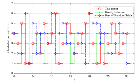
Figure 2: The actuator schedules using different methods.

Interestingly, from the solution to Problem 4 shown in Fig. 3, we notice that the actuator of the $1$-st node is hardly used since the values of $\theta^{1}_{t}$’s are in orders of magnitude smaller than that for the rest of the nodes for all $t$. This is in contrast with the schedule we found in Fig. 2 where actuator $1$ is scheduled for several time instances ($\sim 17$% of the time) by Algorithm 1. Actuator 2 is used the least by Algorithm 1 in Fig. 2, however, in Fig. 3 we notice that $\theta^{2}_{t}$ is not the least among all $\theta^{i}_{t}$’s. While one might be tempted to only use actuators 3 and 4 since the corresponding $\theta^{i}_{t}$ values are the highest ones in Fig. 3, however, such restriction leads to a cost of 108.5531, which is higher than what our method found. This indeed validates our statements in Remark 3.

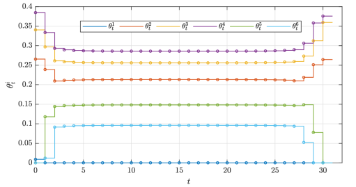
Figure 3: Optimal $\theta^{i}_{t}$ from Problem 4. For all $t$, we obtained $\theta^{5}_{t}=\theta^{6}_{t}$, and hence they are not distinguishable in the figure.

Next, in order to compare the performance of our proposed approach with randomly generated schedules and a greedy selection approach. We randomly selected 50,000 schedules and computed the cost corresponding to these schedules. The resulting cost distribution from the schedules are plotted in Fig. 4 and the minimum cost out of these 50,000 trials is 102.0693.

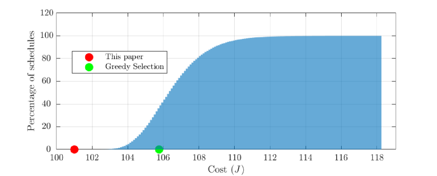
Figure 4: x-axis: Cost ($J$), y-axis: Percentage of the randomly generated trials which produced a cost less than or equal to the value on the x-axis.

Evaluation of the 50,000 random trials took 34.65 seconds whereas our approach (convex optimization plus trajectory tracking) took 2.5 seconds, which is an order of magnitude less time. For the greedy approach, at each time instance we greedily selected the actuator that provides the minimum cost for that time stage. This approach is fast ($<1$ sec) but the performance is the worst (see. Fig. 4).

VI Conclusions

In this letter, we have studied the problem of actuator scheduling for stochastic linear NCSs. In particular, we have considered the case that only one actuator is active at each time. We have proposed a convex relaxation and used its solution as a reference for obtaining a suboptimal tracking algorithm for solving the actuator scheduling problem. Suboptimality guarantees for the proposed algorithm have been provided using dynamic programming arguments. We have also discussed the extensions on the cases with multiple actuator scheduling and actuation costs.

References

- [1] J. P. Hespanha, P. Naghshtabrizi, and Y. Xu, “A survey of recent results in networked control systems,” Proceedings of the IEEE, vol. 95, no. 1, pp. 138–162, 2007.
- [2] G. C. Walsh and H. Ye, “Scheduling of networked control systems,” IEEE control systems magazine, vol. 21, no. 1, pp. 57–65, 2001.
- [3] J. S. Baras and A. Bensoussan, “Sensor scheduling problems,” in Proc. of the 27th IEEE Conference on Decision and Control (CDC), 1988.
- [4] L.-W. Yeh, C.-Y. Lu, C.-W. Kou, Y.-C. Tseng, and C.-W. Yi, “Autonomous light control by wireless sensor and actuator networks,” IEEE Sensors Journal, vol. 10, no. 6, pp. 1029–1041, 2010.
- [5] J. Chen, X. Cao, P. Cheng, Y. Xiao, and Y. Sun, “Distributed collaborative control for industrial automation with wireless sensor and actuator networks,” IEEE Transactions on Industrial Electronics, vol. 57, no. 12, pp. 4219–4230, 2010.
- [6] V. Gupta, T. H. Chung, B. Hassibi, and R. M. Murray, “On a stochastic sensor selection algorithm with applications in sensor scheduling and sensor coverage,” Automatica, vol. 42, no. 2, pp. 251–260, 2006.
- [7] M. P. Vitus, W. Zhang, A. Abate, J. Hu, and C. J. Tomlin, “On efficient sensor scheduling for linear dynamical systems,” Automatica, vol. 48, no. 10, pp. 2482–2493, 2012.
- [8] V. Tzoumas, L. Carlone, G. J. Pappas, and A. Jadbabaie, “LQG control and sensing co-design,” IEEE Transactions on Automatic Control, vol. 66, no. 4, pp. 1468–1483, 2021.
- [9] D. Maity, D. Hartman, and J. S. Baras, “Sensor scheduling for linear systems: a covariance tracking approach,” Automatica, vol. 136, p. 110078, 2022.
- [10] F. Pasqualetti, S. Zampieri, and F. Bullo, “Controllability metrics, limitations and algorithms for complex networks,” IEEE Transactions on Control of Network Systems, vol. 1, no. 1, pp. 40–52, 2014.
- [11] T. H. Summers and J. Lygeros, “Optimal sensor and actuator placement in complex dynamical networks,” IFAC Proceedings Volumes, vol. 47, no. 3, pp. 3784–3789, 2014.
- [12] F. L. Cortesi, T. H. Summers, and J. Lygeros, “Submodularity of energy related controllability metrics,” in 53rd IEEE conference on decision and control. IEEE, 2014, pp. 2883–2888.
- [13] M. Siami, A. Olshevsky, and A. Jadbabaie, “Deterministic and randomized actuator scheduling with guaranteed performance bounds,” IEEE Transactions on Automatic Control, vol. 66, no. 4, pp. 1686–1701, 2021.
- [14] C. Maheshwari, S. Srikant, and D. Chatterjee, “Stabilization under round-robin scheduling of control inputs in nonlinear systems,” Automatica, vol. 134, p. 109912, 2021.
- [15] E. Nozari, F. Pasqualetti, and J. Cortés, “Time-invariant versus time-varying actuator scheduling in complex networks,” in 2017 American Control Conference (ACC). IEEE, 2017, pp. 4995–5000.
- [16] L. Shi, Y. Yuan, and J. Chen, “Finite horizon LQR control with limited controller-system communication,” IEEE Transactions on Automatic Control, vol. 58, no. 7, pp. 1835–1841, 2013.
- [17] L. Mo, P. You, X. Cao, Y. Song, and A. Kritikakou, “Event-driven joint mobile actuators scheduling and control in cyber-physical systems,” IEEE Transactions on Industrial Informatics, vol. 15, no. 11, pp. 5877–5891, 2019.
- [18] P. Bommannavar and T. Basar, “Optimal control with limited control actions and lossy transmissions,” in 2008 47th IEEE conference on decision and control. IEEE, 2008, pp. 2032–2037.
- [19] D. Bertsekas, Dynamic Programming and Optimal Control: Volume I. Athena scientific, 2012.
- [20] V. Tzoumas, A. Jadbabaie, and G. J. Pappas, “Near-optimal sensor scheduling for batch state estimation: Complexity, algorithms, and limits,” in 55th IEEE Conference on Decision and Control, Las Vegas, USA, 2016, pp. 2695–2702.
- [21] T. Gally, M. E. Pfetsch, and S. Ulbrich, “A framework for solving mixed-integer semidefinite programs,” Optimization Methods and Software, vol. 33, no. 3, pp. 594–632, 2018.
- [22] B. Sinopoli, L. Schenato, M. Franceschetti, K. Poolla, M. I. Jordan, and S. S. Sastry, “Kalman filtering with intermittent observations,” IEEE transactions on Automatic Control, vol. 49, no. 9, pp. 1453–1464, 2004.