The infrared behavior of tame two-field cosmological models

Abstract

We study the first order infared behavior of tame hyperbolizable two-field cosmological models, defined as those classical two-field models whose scalar manifold is a connected, oriented and topologically finite hyperbolizable Riemann surface $(\Sigma,\mathcal{G})$ and whose scalar potential $\Phi$ admits a positive and Morse extension to the end compactification of $\Sigma$. We achieve this by determining the universal forms of the asymptotic gradient flow of the classical effective potential $V$ with respect to the uniformizing metric $G$ near all interior critical points and ends of $\Sigma$, finding that some of the latter act like fictitious but exotic stationary points of the gradient flow. We also compare these results with numerical studies of cosmological orbits. For critical cusp ends, we find that cosmological curves have transient quasiperiodic behavior but are eventually attracted or repelled by the cusp along principal geodesic orbits determined by the extended effective potential. This behavior is approximated in the infrared by that of gradient flow curves near the cusp.

Introduction

Two-field cosmological models provide the simplest testing ground for multifield cosmological dynamics. Such models are important for connecting cosmology with fundamental theories of gravity and matter, since the effective description of the generic string or M-theory compactification contains many moduli fields. In particular, multifield models are crucial in cosmological applications of the swampland program V ; OV ; BCV ; BCMV , as pointed out for example in AP ; OOSV ; GK . They may also afford a unified description of inflation, dark matter and dark energy AL .

A two-field cosmological model is parameterized by the rescaled Planck mass $M_{0}\stackrel{{\scriptstyle{\rm def.}}}{{=}}M\sqrt{\frac{2}{3}}$ (where $M$ is the reduced Planck mass) and by its scalar triple $(\Sigma,\mathcal{G},\Phi)$, where the generally non-compact borderless connected surface $\Sigma$ is the target manifold for the scalar fields, $\mathcal{G}$ is the scalar field metric and $\Phi$ is the scalar potential. To ensure conservation of energy, one requires that $\mathcal{G}$ is complete; we also assume that $\Phi$ is strictly positive. In ren , we used a dynamical RG flow analysis and the uniformization theorem of Poincaré to show that two-field models whose scalar field metric has constant Gaussian curvature $K$ equal to $-1$, $0$ or $+1$ give distinguished representatives for the IR universality classes of all two-field cosmological models. More precisely, the first order IR approximants of cosmological orbits for the model parameterized by $(M_{0},\Sigma,\mathcal{G},\Phi)$ coincide with those of the model parameterized by $(M_{0},\Sigma,G,\Phi)$, where $G$ is the uniformizing metric of $\mathcal{G}$. Moreover, these approximants coincide with the gradient flow orbits of $(\Sigma,G,V)$, where $V\stackrel{{\scriptstyle{\rm def.}}}{{=}}M_{0}\sqrt{2\Phi}$ is the classical effective potential of the model. In particular, IR universality classes depend only on the scalar triple $(\Sigma,G,V)$. This result allows for systematic studies of two-field cosmological models belonging to a fixed IR universality class by using the infrared expansion of cosmological curves outlined in ren . The reduction to uniformized models, defined as those whose scalar field metric has Gaussian curvature $K$ equal to $-1$, $0$ or $+1$ serves as an organizing principle for the infrared expansion, the first order of which is captured by the gradient flow of $(\Sigma,G,V)$.

The case $K=-1$ is generic and obtains when the topology of $\Sigma$ is of general type; for such models, the uniformizing metric is hyperbolic. The few exceptions to this situation arise when $\Sigma$ is of special type, namely diffeomorphic to $\mathbb{R}^{2}$, the two-sphere $\mathrm{S}^{2}$, the real projective plane $\mathbb{R}\mathbb{P}^{2}$, the two torus $\mathrm{T}^{2}$, the open Klein bottle $\mathrm{K}^{2}=\mathbb{R}\mathbb{P}^{2}\times\mathbb{R}\mathbb{P}^{2}\simeq\mathrm{T}^{2}/\mathbb{Z}_{2}$, the open annulus $\mathrm{A}^{2}$ or the open Möbius strip $\mathrm{M}^{2}\simeq\mathrm{A}^{2}/\mathbb{Z}_{2}$. When $\Sigma$ is diffeomorphic to $\mathrm{S}^{2}$ or $\mathbb{R}\mathbb{P}^{2}$, the uniformizing metric has Gaussian curvature $+1$, while when it is diffeomorphic to a torus or Klein bottle the uniformizing metric is flat and complete. When $\Sigma$ is of exceptional type, i.e. diffeomorphic to $\mathbb{R}^{2}$, $\mathrm{A}^{2}$ or $\mathrm{M}^{2}$, the metric $\mathcal{G}$ uniformizes to a complete flat metric or to a hyperbolic metric depending on its conformal class. The cosmological model, its scalar field metric $\mathcal{G}$ and the conformal class of the latter are called hyperbolizable when $\mathcal{G}$ uniformizes to a hyperbolic metric. Thus hyperbolizable models comprise all two-field models whose target is of general type as well as those models whose target is exceptional (i.e diffeomorphic with $\mathbb{R}^{2}$, $\mathrm{A}^{2}$ or $\mathrm{M}^{2}$) and for which $\mathcal{G}$ belongs to a hyperbolizable conformal class. The uniformized form $(M_{0},\Sigma,G,\Phi)$ of a hyperbolizable model is a two field generalized $\alpha$-attractor model in the sense of genalpha . Some aspects of such models were investigated previously in elem ; modular ; Noether1 ; Noether2 ; Hesse ; Lilia1 ; Lilia2 (see unif ; Nis ; Tim19 ; LiliaRev for brief reviews).

In this paper, we study the infrared behavior of hyperbolizable two-field models with certain technical assumptions on the topology of $\Sigma$ and on the scalar potential $\Phi$. Namely, we assume that $\Sigma$ is oriented and topologically finite in the sense that it has finitely-generated fundamental group. When $\Sigma$ is non-compact, this condition insures that it has a finite number of Freudenthal ends Freudenthal1 ; Freudenthal2 ; Freudenthal3 and that its end (a.k.a. Kerekjarto-Stoilow Kerekjarto ; Stoilow ; Richards ) compactification $\widehat{\Sigma}$ is a smooth and oriented compact surface. Thus $\Sigma$ is recovered from $\widehat{\Sigma}$ by removing a finite number of points. We also assume that $\Phi$ admits a smooth extension ${\hat{\Phi}}$ to $\widehat{\Sigma}$ which is a strictly-positive Morse function defined on $\widehat{\Sigma}$. A two-field cosmological model is called tame when these conditions are satisfied.

To first order in the scale expansion of ren , the IR limit of a tame two-field model is given by the gradient flow of the classical effective potential $V=M_{0}\sqrt{2\Phi}$ on the geometrically finite hyperbolic surface $(\Sigma,G)$. Since the future limit points of cosmological curves and of the gradient flow curves of $(\Sigma,G,V)$ are critical points of $\Phi$ or Freudenthal ends of $\Sigma$, the asymptotic behavior of such curves for late cosmological times is determined by the form of $G$ and $V$ near such points. The form of $G$ near critical points follows from the fact that any hyperbolic surface is locally isometric with a domain of the Poincaré disk, while that near each end follows from the uniformization of geometrically finite hyperbolic surfaces. Since the Morse assumption on the extended potential determines its asymptotic form near the points of interest, this allows us to derive closed form expressions for the asymptotic gradient flow and hence to describe the infrared phases of such models in the sense of ren . In particular, we find that the asymptotic gradient flow of $(\Sigma,G,V)$ near each end which is a critical point of the extended potential can be expressed using the incomplete gamma function of order two and certain constants which depend on the type of end under consideration and on the (appropriately-defined) principal values of the extended effective potential $\widehat{V}$ at that end. We also find that flaring ends which are not critical points of $\widehat{V}$ act like fictitious but non-standard stationary points of the effective gradient flow. While the local form near the critical points of $V$ is standard (since they are hyperbolic stationary points Palis ; Katok of the cosmological and gradient flow), the asymptotic behavior near Freudenthal ends is exotic in that some of the ends act like fictitious stationary points with unusual characteristics. For example, the stable and unstable manifolds of an end under the gradient flow of $(\Sigma,G,V)$ can have dimensions which differ from those of hyperbolic stationary points of dynamical systems.

We compare these results with numerical computations of cosmological curves near the points of interest. We find particularly interesting behavior near cusp ends, around which generic cosmological trajectories tend to spiral a large number of times before either “falling into the cusp” or being “repelled” back toward the compact core of $\Sigma$ along principal geodesic orbits determined by $V$. In particular, cusp ends lead naturally to “fast turn” behavior of cosmological curves, a phenomenon which we already illustrated in our previous analysis of the hyperbolic triply punctured sphere (see modular ).

The paper is organized as follows. In Section 1, we briefly recall the global description of multifield cosmological models through a second order geometric ODE and their first order infrared approximation introduced in ren . Section 2 defines tame two-field cosmological models, describes the critical points of their extended potential and discusses principal coordinates centered at ends. In the same section, we recall the form of the hyperbolic metric $G$ in a canonical vicinity of an end and extract its asymptotic behavior near each type of end. Section 3 discusses the behavior of cosmological curves and their first order IR approximants near interior critical points. Section 4 performs the asymptotic analysis of gradient flow curves and compares it with numerical results for cosmological curves near those ends of $\Sigma$ which are noncritical for the extended scalar potential, while Section 5 performs the same analysis for critical ends. Section 6 presents our conclusions and some directions for further research. The appendix gives some details of the computation of cosmological curves near interior critical points and near Freudenthal ends.

Notations and conventions.

All surfaces $\Sigma$ considered in this paper are connected, smooth, Hausdorff and paracompact. If $V$ is a smooth real-valued function defined on $\Sigma$, we denote by:

$$\mathrm{Crit}V\stackrel{{\scriptstyle{\rm def.}}}{{=}}\{c\in\Sigma|(\mathrm{d}V)(c)=0\}$$

the set of its critical points. For any $c\in\mathrm{Crit}V$, we denote by $\mathrm{Hess}(V)(c)\in\mathrm{Sym}^{2}(T^{\ast}_{c}\Sigma)$ the Hessian of $V$ at $c$, which is a well-defined and coordinate independent symmetric bilinear form on the tangent space $T_{c}\Sigma$. Given a metric $\mathcal{G}$ on $\Sigma$, we denote by:

$$\mathrm{Hess}_{\mathcal{G}}(V)\stackrel{{\scriptstyle{\rm def.}}}{{=}}\nabla\mathrm{d}V\in\Gamma(\Sigma,\mathrm{Sym}^{2}(T^{\ast}\Sigma))$$

the covariant Hessian tensor of $V$ relative to $\mathcal{G}$, where $\nabla$ is the Levi-Civita connection of $\mathcal{G}$. This symmetric tensor has the following local expression in coordinates $(x^{1},x^{2})$ on $\Sigma$:

$$\mathrm{Hess}_{\mathcal{G}}(V)=(\partial_{i}\partial_{j}-\Gamma^{k}_{ij}(x)\partial_{k})V\mathrm{d}x^{i}\otimes\mathrm{d}x^{j}~{}~{},$$

where $\Gamma^{k}_{ij}(x)$ are the Christoffel symbols of $\mathcal{G}$. For any critical point $c\in\mathrm{Crit}V$, we have $\mathrm{Hess}_{\mathcal{G}}(V)(c)=\mathrm{Hess}(V)(c)$. Recall that a critical point $c$ of $V$ is called nondegenerate if $\mathrm{Hess}(V)(c)$ is a non-degenerate bilinear form. When $V$ is a Morse function (i.e. has only non-degenerate critical points), the set $\mathrm{Crit}V$ is discrete.

We denote by $\widehat{\Sigma}$ the Freudenthal (a.k.a. end) compactification of $\Sigma$, which is a compact Hausdorff topological space containing $\Sigma$ (see Freudenthal1 ; Freudenthal2 ; Freudenthal3 ). We say that $\Sigma$ is topologically finite if its fundamental group is finitely generated. In this case, $\Sigma$ has a finite number of Freudenthal ends and $\widehat{\Sigma}$ is a smooth compact surface. In this situation, we say that $V$ is globally well-behaved on $\Sigma$ if it admits a smooth extension $\widehat{V}$ to $\widehat{\Sigma}$. A metric $\mathcal{G}$ on $\Sigma$ is called hyperbolic if it is complete and of constant Gaussian curvature equal to $-1$.

1 Two-field cosmological models and their IR approximants

Recall that a two-field cosmological model is a classical cosmological model with two scalar fields derived from the following action on a spacetime with topology $\mathbb{R}^{4}$:

$$S[g,\varphi]=\int\mathrm{vol}_{g}\mathcal{L}[g,\varphi]~{}~{},$$ (1)

where:

$$\mathcal{L}[g,\varphi]=\frac{M^{2}}{2}\mathrm{R}(g)-\frac{1}{2}\mathrm{Tr}_{g}\varphi^{\ast}(\mathcal{G})-\Phi\circ\varphi~{}~{}.$$ (2)

Here $M$ is the reduced Planck mass, $g$ is the spacetime metric on $\mathbb{R}^{4}$ (taken to be of “mostly plus”) signature, while $\mathrm{vol}_{g}$ and $\mathrm{R}(g)$ are the volume form and Ricci scalar of $g$. The scalar fields are described by a smooth map $\varphi:\mathbb{R}^{4}\rightarrow\Sigma$, where $\Sigma$ is a (generally non-compact) smooth and connected paracompact surface without boundary which is endowed with a smooth Riemannian metric $\mathcal{G}$, while $\Phi:\Sigma\rightarrow\mathbb{R}$ is a smooth function which plays the role of potential for the scalar fields. We require that $\mathcal{G}$ is complete to ensure conservation of energy. For simplicity, we also assume that $\Phi$ is strictly positive on $\Sigma$. Notice that the model is parameterized by the quadruplet $\mathfrak{M}\stackrel{{\scriptstyle{\rm def.}}}{{=}}(M_{0},\Sigma,\mathcal{G},\Phi)$, where:

$$M_{0}\stackrel{{\scriptstyle{\rm def.}}}{{=}}M\sqrt{\frac{2}{3}}$$

is the rescaled Planck mass.

1.1 The cosmological equation

The two-field model parameterized by $\mathfrak{M}$ is obtained by assuming that $g$ is an FLRW metric with flat spatial section:

$$\mathrm{d}s^{2}_{g}=-\mathrm{d}t^{2}+a(t)^{2}\sum_{i=1}^{3}\mathrm{d}x_{i}^{2}$$ (3)

(where $a(t)>0$) and that $\varphi$ depends only on the cosmological time $t\stackrel{{\scriptstyle{\rm def.}}}{{=}}x^{0}$. One sets:

$$H(t)\stackrel{{\scriptstyle{\rm def.}}}{{=}}\frac{\dot{a}(t)}{a(t)}~{}~{},$$

where the dot indicates derivation with respect to $t$. When $H>0$ (which we assume throughout), the variational equations of (1) reduce to the cosmological equation:

$$\nabla_{t}\dot{\varphi}(t)+\frac{1}{M_{0}}\left[||\dot{\varphi}(t)||_{\mathcal{G}}^{2}+2\Phi(\varphi(t))\right]^{1/2}\dot{\varphi}(t)+(\mathrm{grad}_{\mathcal{G}}\Phi)(\varphi(t))=0$$ (4)

together with the condition:

$$H(t)=H_{\varphi}(t)~{}~{},$$ (5)

where the Hubble parameter of $\varphi$ is defined through:

$$H_{\varphi}(t)\stackrel{{\scriptstyle{\rm def.}}}{{=}}\frac{1}{3M_{0}}\left[||\dot{\varphi}(t)||_{\mathcal{G}}^{2}+2\Phi(\varphi(t))\right]^{1/2}~{}~{}.$$ (6)

Here $\nabla_{t}\stackrel{{\scriptstyle{\rm def.}}}{{=}}\nabla_{\dot{\varphi}(t)}$ is the covariant derivative with respect to the tangent vector $\dot{\varphi}(t)\in T_{\varphi(t)}\Sigma$, which takes the following form in local coordinates on $\Sigma$:

$$\nabla_{t}\dot{\varphi}^{i}(t)=\ddot{\varphi}^{i}(t)+\Gamma^{i}_{jk}(\varphi(t))\dot{\varphi}^{j}(t)\dot{\varphi}^{k}(t)~{}~{},$$

where $\Gamma^{i}_{jk}$ are the Christoffel symbols of $\mathcal{G}$. The solutions $\varphi:I\rightarrow\Sigma$ of (4) (where $I$ is a non-degenerate interval) are called cosmological curves, while their images in $\Sigma$ are called cosmological orbits. Given a cosmological curve $\varphi$, relation (61) determines $a$ up to a multiplicative constant. The cosmological equation can be reduced to first order by passing to the tangent bundle of $T\Sigma$ (see SLK ). More precisely, (4) is equivalent with the integral curve equation of a semispray (a.k.a. second order vector field) $S$ defined on $T\Sigma$ which is called the cosmological semispray of the model (see ren ). The flow of this vector field on the total space of $T\Sigma$ is called the cosmological flow.

Remark 1.1.

The cosmological equation can be written as:

$$\nabla_{t}\dot{\varphi}(t)+\left[||\dot{\varphi}(t)||_{\mathcal{G}_{0}}^{2}+2\Phi_{0}(\varphi(t))\right]^{1/2}\dot{\varphi}(t)+(\mathrm{grad}_{\mathcal{G}_{0}}\Phi_{0})(\varphi(t))=0~{}~{},$$

where we defined the rescaled scalar field metric and rescaled scalar potential by:

$$\mathcal{G}_{0}\stackrel{{\scriptstyle{\rm def.}}}{{=}}\frac{1}{M_{0}^{2}}\mathcal{G}~{}~{}\mathrm{and}~{}~{}\Phi_{0}\stackrel{{\scriptstyle{\rm def.}}}{{=}}\ \frac{1}{M_{0}^{2}}\Phi~{}~{}.$$

Moreover, (6) reads:

$$H_{\varphi}(t)=\frac{1}{3}\left[||\dot{\varphi}(t)||_{\mathcal{G}_{0}}^{2}+2\Phi_{0}(\varphi(t))\right]^{1/2}~{}~{}.$$

Hence the cosmological curves and their Hubble parameters depend only on the rescaled scalar triple $(\Sigma,\mathcal{G}_{0},\Phi_{0})$.

1.2 Uniformized models and first order IR approximants

Consider a cosmological curve $\varphi:I\rightarrow\Sigma$ of the model parameterized by $(M_{0},\Sigma,\mathcal{G},\Phi)$, where we can assume that $0\in I$ by shifting the cosmological time since the cosmological equation is autonomous. Define the classical effective potential $V$ of the model by:

$$V\stackrel{{\scriptstyle{\rm def.}}}{{=}}M_{0}\sqrt{2\Phi}~{}~{}.$$

The dynamical RG flow analysis of ren shows that the first order IR approximant of $\varphi$ is the gradient flow curve $\eta$ of the scalar triple $(\Sigma,\mathcal{G},V)$ which satisfies the initial condition:

$$\eta(0)=\varphi(0)~{}~{}.$$ (7)

Since the gradient flow of $V$ is invariant under Weyl transformations of $\mathcal{G}$ up to increasing reparameterization of the gradient flow curves, the uniformization theorem of Poincaré allows us to replace $\mathcal{G}$ with its uniformizing metric $G$ without changing the oriented gradient flow orbits. Hence the first order IR approximation of cosmological flow orbits is given by the gradient flow orbits of the hyperbolic scalar triple $(\Sigma,G,V)$. Thus the original model parameterized by $(M_{0},\Sigma,\mathcal{G},\Phi)$ and the uniformized model parameterized by $(M_{0},\Sigma,G,\Phi)$ have the same first order IR orbits. The uniformized model provides a distinguished representative of the IR universality class of the original model as defined in ren . Moreover, this universality class depends only on the scalar triple $(\Sigma,G,V)$. Notice that the initial condition (7) for first order IR approximants is invariant under reparameterizations since both the cosmological and gradient flow equations are autonomous and we can shift parameters to ensure that (7) does not change. From now on, we work exclusively with the uniformized model $(M_{0},\Sigma,G,\Phi)$ and its scalar triple $(\Sigma,G,V)$, whose gradient flow we call the effective gradient flow.

Since the gradient flow equation of $(\Sigma,G,V)$:

$$\dot{\eta}(t)=-(\mathrm{grad}_{G}V)(\eta(t))$$

is a first order ODE, the degree of the cosmological equation drops by one in the first order IR approximation. As a result, the tangent vector to $\eta$ is constrained to lie within the gradient flow shell $\mathrm{Grad}_{G}V$ of $(\Sigma,G,V)$. The latter is the closed submanifold of $T\Sigma$ defined as the graph of the vector field $-\mathrm{grad}_{G}V$:

$$\mathrm{Grad}_{G}V\stackrel{{\scriptstyle{\rm def.}}}{{=}}\{u\in T\Sigma~{}|~{}u=-(\mathrm{grad}_{G}V)(\pi(u))\}~{}~{},$$

where $\pi:T\Sigma\rightarrow\Sigma$ is the tangent bundle projection. In particular, the cosmological flow of the uniformized model (which is defined on $T\Sigma$) becomes confined to $\mathrm{Grad}_{G}V$ in this approximation. In this order of the IR expansion, the tangent vector $\dot{\eta}(0)$ is constrained to equal $-(\mathrm{grad}_{G}V)(\eta(0))$ and cannot be specified independently; one has to consider higher orders of the expansion to obtain an approximant of the cosmological flow which is defined on the entirety of $T\Sigma$. In particular, the IR approximation is rather coarse.

A cosmological curve $\varphi$ is called infrared optimal if its speed at $t=0$ lies in gradient flow shell of $(\Sigma,G,V)$, i.e. if $\varphi$ satisfies the condition:

$$\dot{\varphi}(0)=-(\mathrm{grad}_{G}V)(\varphi(0))~{}~{}.$$

The first order IR approximant $\eta$ of an infrared optimal cosmological curve osculates in first order to $\varphi$ at $t=0$. Thus $\eta(t)$ is a first order asymptotic approximant of $\varphi(t)$ for $|t|\ll 1$. The covariant acceleration $\nabla_{t}\dot{\varphi}(0)$ of $\varphi$ at $t=0$ need not agree with that of $\eta$ (which is determined by the gradient flow equation). As a consequence, $\varphi(t)$ and $\eta(t)$ can differ already to the second order in $t$. The two curves osculate in second order at $t=0$ only if $G$ and $\Phi$ satisfy a certain condition at the initial point $\varphi(0)$ (see ren ). In particular, the IR approximation of an infrared optimal cosmological curve can be expected to be accurate only for sufficiently small cosmological times. For cosmological curves which are not IR optimal, the approximation can be accurate only when the speed of the curve at $t=0$ is sufficiently close to the gradient flow shell of $(\Sigma,\mathcal{G},V)$. Despite these limitations, the first order IR approximation provides an important conceptual tool for classifying multifield cosmological models into IR universality classes and gives a useful picture of the low frequency behavior of cosmological curves (see ren ).

Remark 1.2.

The transformation $G\rightarrow G_{0}=\frac{1}{M_{0}^{2}}G$, $\Phi\rightarrow\Phi_{0}=\frac{1}{M_{0}^{2}}\Phi$ replaces $(\Sigma,G,V)$ with $(\Sigma,G_{0},V_{0})$, where $V_{0}=M_{0}\sqrt{2\Phi_{0}}=\sqrt{2\Phi}=\frac{1}{M_{0}}V$. Since $\mathrm{grad}_{G_{0}}V_{0}=M_{0}\mathrm{grad}_{G}V$, the gradient flow shell of $(\Sigma_{0},G_{0},V_{0})$ differs from that of $(\Sigma,G,V)$ by a constant rescaling in the fiber directions. This can be absorbed by a constant reparameterization of the gradient flow curves and hence does not affect the gradient flow orbits.

2 Hyperbolizable tame two-field models

The results of ren allow us to describe the infrared behavior of two-field models under certain assumptions on the scalar manifold and potential. Throughout this section, we consider a hyperbolizable model parameterized by $(M_{0},\Sigma,\mathcal{G},\Phi)$ and let $G$ be the hyperbolization of $\mathcal{G}$ and $V\stackrel{{\scriptstyle{\rm def.}}}{{=}}M_{0}\sqrt{2\Phi}$.

2.1 The tameness conditions

Recall that adding the Freudenthal ends to $\Sigma$ produces its end compactification $\widehat{\Sigma}$, where each point of the set:

$$\mathrm{Ends}(\Sigma)\stackrel{{\scriptstyle{\rm def.}}}{{=}}\widehat{\Sigma}\setminus\Sigma$$

corresponds to an end. When endowed with its natural topology, $\widehat{\Sigma}$ is the classical compactification of surfaces considered by Kerekjarto and Stoilow Kerekjarto ; Stoilow , which was clarified further and extended to the unoriented case by Richards Richards ; it coincides with Freudenthal’s end compactification of manifolds for the case of dimension two. In general, the set of ends $\mathrm{Ends}(\Sigma)$ can be infinite and rather complicated (it is a totally disconnected space which can be a Cantor space). Moreover, the scalar potential $\Phi$ (and the effective potential $V$) can have complicated asymptotic behavior near each end; in particular, they may fail to extend to smooth functions on $\widehat{\Sigma}$. Furthermore, $\Phi$ (and thus $V$) may have non-isolated critical points on $\Sigma$. To obtain a tractable set of models, we make the following

Assumptions.

1. $\Sigma$ is oriented and topologically finite in the sense that its fundamental group $\pi_{1}(\Sigma)$ is finitely-generated. This implies that $\Sigma$ has finite genus and a finite number of ends and that its end compactification $\widehat{\Sigma}$ is a compact smooth surface. Notice that $(\Sigma,G)$ need not have finite area.

2. The scalar potential $\Phi$ is globally well-behaved, i.e. $\Phi$ admits a smooth extension ${\hat{\Phi}}$ to $\widehat{\Sigma}$. We require that ${\hat{\Phi}}$ is strictly positive on $\widehat{\Sigma}$, which means that the limit of $\Phi$ at each end of $\Sigma$ is a strictly positive number.

3. The extended potential ${\hat{\Phi}}$ is a Morse function on $\widehat{\Sigma}$ (in particular, $\Phi$ is a Morse function on $\Sigma$).

Definition 2.1.

A hyperbolic two-dimensional scalar triple $(\Sigma,\mathcal{G},\Phi)$ is called tame if it satisfies conditions $1$, $2$ and $3$ above. A two-field cosmological model with tame scalar triple is called tame.

Remark 2.2.

It may seem at first sight that our tameness assumptions could reduce the study of the IR behavior of cosmological curves to an application of known results from Morse theory MB ; Bott and from the theory of gradient flows. However this is not the case because the metrics $\mathcal{G}$ and $G$ do not extend to the end compactification of $\Sigma$ and because the vector field $\mathrm{grad}_{G}V$ is singular at the ends. On the other hand, the flow of $\mathrm{grad}_{G}V$ on the non-compact surface $\Sigma$ is not amenable to ordinary Morse theory, which assumes a compact manifold. One might hope that some version of Morse theory on manifolds with boundary (see KM ; Laudenbach ; Akaho ) could apply to the conformal compactification of $(\Sigma,G)$. However, the assumptions made in common versions of that theory are not satisfied in our case. As already shown in genalpha , Morse theoretic results are nevertheless useful for relating the indices of the critical points of ${\hat{\Phi}}$ to the topology of $\Sigma$ – a relation which can be used in principle to constrain the topology of $\Sigma$ using cosmological observations.

2.2 Interior critical points. Critical and noncritical ends

The assumption that $\Sigma$ is topologically finite implies that the set of ends $\mathrm{Ends}(\Sigma)$ is finite, while the assumption that ${\hat{\Phi}}$ is Morse constrains the asymptotic behavior of $\Phi$ at the ends of $\Sigma$. Notice that the extended potential is uniquely determined by $\Phi$, since continuity of ${\hat{\Phi}}$ implies:

$${\hat{\Phi}}({\bf e})=\lim_{\Sigma\ni m\rightarrow{\bf e}}\Phi(m)~{}~{}\forall{\bf e}\in\mathrm{Ends}(\Sigma)~{}~{}.$$

Also notice that ${\hat{\Phi}}$ (hence also $\Phi$) is bounded since it is continuous while $\widehat{\Sigma}$ is compact. The condition that ${\hat{\Phi}}$ is Morse implies that its critical points are isolated. Since $\widehat{\Sigma}$ is compact, it follows that the set:

$$\mathrm{Crit}{\hat{\Phi}}\stackrel{{\scriptstyle{\rm def.}}}{{=}}\{c\in\widehat{\Sigma}|(\mathrm{d}{\hat{\Phi}})(c)=0\}$$

is finite. Since we assume that ${\hat{\Phi}}$ is strictly positive on $\widehat{\Sigma}$, the classical effective potential $V=M_{0}\sqrt{2\Phi}$ is also globally well-behaved, i.e. admits a smooth extension $\widehat{V}$ to $\widehat{\Sigma}$, which is given by:

$$\widehat{V}=M_{0}\sqrt{2{\hat{\Phi}}}~{}~{}.$$

Moreover, $\widehat{V}$ has the same critical points as ${\hat{\Phi}}$:

$$\mathrm{Crit}\widehat{V}=\mathrm{Crit}{\hat{\Phi}}~{}~{}.$$

Since $V$ is the restriction of $\widehat{V}$ to $\Sigma$, the critical points of $V$ coincide with the interior critical points of $\widehat{V}$ (and ${\hat{\Phi}}$), i.e. those critical points which lie on $\Sigma$:

$$\mathrm{Crit}V=\mathrm{Crit}\Phi=\Sigma\cap\mathrm{Crit}\widehat{V}=\Sigma\cap\mathrm{Crit}{\hat{\Phi}}~{}~{}.$$

Let:

$$\mathrm{Crit}_{\infty}V=\mathrm{Crit}_{\infty}\Phi\stackrel{{\scriptstyle{\rm def.}}}{{=}}\mathrm{Ends}(\Sigma)\cap\mathrm{Crit}\widehat{V}=\mathrm{Ends}(\Sigma)\cap\mathrm{Crit}{\hat{\Phi}}$$

be the set of critical ends (or “critical points at infinity”), i.e. those critical points of the extended potential which are also ends of $\Sigma$. We have the disjoint union decomposition:

$$\mathrm{Crit}\widehat{V}=\mathrm{Crit}V\sqcup\mathrm{Crit}_{\infty}V~{}~{}.$$

Finally, an end of $\Sigma$ which is not a critical point of ${\hat{\Phi}}$ (and hence of $\widehat{V}$) will be called a noncritical end. Such ends form the set $\mathrm{Ends}(\Sigma)\setminus\mathrm{Crit}_{\infty}(V)$. We denote interior critical points by ${\bf c}$ and arbitrary critical points of $\widehat{V}$ by $c$; the latter can be interior critical points or critical ends. Finally, we denote by ${\bf e}$ the ends of $\Sigma$. To describe the early and late time behavior of the gradient flow of $(\Sigma,G,V)$, we must study the asymptotic form of this flow near the interior critical points as well as near all ends of $\Sigma$.

2.3 Stable and unstable manifolds under the effective gradient flow

For any maximal gradient flow curve $\eta:(a_{-},a_{+})\rightarrow\Sigma$ of $(\Sigma,G,V)$, we denote by:

$$\mathrm{lim}_{\alpha}\eta\stackrel{{\scriptstyle{\rm def.}}}{{=}}\lim_{t\rightarrow a_{-}}\eta(t)\in\widehat{\Sigma}~{}~{}\mathrm{and}~{}~{}\mathrm{lim}_{\omega}\eta\stackrel{{\scriptstyle{\rm def.}}}{{=}}\lim_{t\rightarrow a_{+}}\eta(t)\in\widehat{\Sigma}$$

its $\alpha$- and $\omega$- limits as a curve in $\widehat{\Sigma}$. Each of these points is either an interior critical point or an end of $\Sigma$.

For any $m\in\Sigma$, let $\eta_{m}$ be the maximal gradient flow curve of $(\Sigma,G,V)$ which satisfies $\eta_{m}(0)=m$. Recall that the stable and unstable manifolds of an interior critical point ${\bf c}\in\mathrm{Crit}V$ under the gradient flow of $(\Sigma,G,V)$ are defined through:

$$\mathcal{S}({\bf c})\stackrel{{\scriptstyle{\rm def.}}}{{=}}\{m\in\Sigma|\mathrm{lim}_{\omega}\eta_{m}(q)={\bf c}\}~{}~{},~{}~{}\mathcal{U}({\bf c})\stackrel{{\scriptstyle{\rm def.}}}{{=}}\{m\in\Sigma|\mathrm{lim}_{\alpha}\eta_{m}(q)={\bf c}\}~{}~{}.$$ (8)

By analogy, we define the stable and unstable manifolds of an end ${\bf e}$ by:

$$\mathcal{S}({\bf e})\stackrel{{\scriptstyle{\rm def.}}}{{=}}\{m\in\Sigma|\mathrm{lim}_{\omega}\eta_{m}(q)={\bf e}\}~{}~{},~{}~{}\mathcal{U}({\bf e})\stackrel{{\scriptstyle{\rm def.}}}{{=}}\{m\in\Sigma|\mathrm{lim}_{\alpha}\eta_{m}(q)={\bf e}\}~{}~{}.$$ (9)

Notice that the stable and unstable manifolds of an end are subsets of $\Sigma$.

2.4 The form of $G$ in a vicinity of an end

Recall (see Borthwick or (genalpha, , Appendix D.6)) that any end ${\bf e}$ of a geometrically-finite and oriented hyperbolic surface $(\Sigma,G)$ admits an open neighborhood $U_{\bf e}\subset\widehat{\Sigma}$ (which is diffeomorphic with a disk) such that the hyperbolic metric $G$ takes a canonical form when restricted to $\dot{U}_{\bf e}\stackrel{{\scriptstyle{\rm def.}}}{{=}}U_{\bf e}\setminus\{{\bf e}\}\subset\Sigma$. More precisely, there exist semigeodesic polar coordinates $(r,\theta)\in\mathbb{R}_{>0}\times\mathrm{S}^{1}$ defined on $\dot{U}_{\bf e}$ in which the hyperbolic metric has the form:

$$\mathrm{d}s_{G}^{2}|_{\dot{U}_{\bf e}}=\mathrm{d}r^{2}+f_{\bf e}(r)\mathrm{d}\theta^{2}~{}~{},$$ (10)

where:

$$f_{\bf e}(r)=\left\{\begin{array}[]{ll}\sinh^{2}(r)&\mbox{if}~{}{\bf e}=\mathrm{plane~{}end}\\ \frac{1}{(2\pi)^{2}}e^{2r}&\mbox{if}~{}{\bf e}=\mathrm{horn~{}end}\\ \frac{\ell^{2}}{(2\pi)^{2}}\cosh^{2}(r)&\mbox{if}~{}{\bf e}=\mathrm{funnel~{}end~{}of~{}circumference}~{}\ell>0\\ \frac{1}{(2\pi)^{2}}e^{-2r}&\mbox{if}~{}{\bf e}=\mathrm{cusp~{}end}\end{array}\right.~{}~{}.$$ (11)

In such coordinates, the end ${\bf e}$ corresponds to $r\rightarrow\infty$. Setting $\zeta\stackrel{{\scriptstyle{\rm def.}}}{{=}}re^{\mathbf{i}\theta}$, the corresponding semigeodesic Cartesian coordinates are defined through:

$$\zeta_{1}\stackrel{{\scriptstyle{\rm def.}}}{{=}}\mathrm{Re}(\zeta)=r\cos\theta~{}~{}\mathrm{and}~{}~{}\zeta_{2}\stackrel{{\scriptstyle{\rm def.}}}{{=}}\mathrm{Im}(\zeta)=r\sin\theta~{}~{}.$$

Plane, horn and funnel ends are called flaring ends. For such ends, the length of horocycles in $(\Sigma,G)$ grows exponentially when one approaches ${\bf e}$. The only non-flaring ends are cusp ends, for which the length of horocycles tends to zero as one approaches the cusp. An oriented geometrically-finite hyperbolic surface is called elementary if it is isometric with the Poincaré disk, the hyperbolic punctured disk or a hyperbolic annulus. A non-elementary oriented geometrically finite hyperbolic surface admits only cusp and funnel ends. The Poincaré disk has a single end which is a plane end. The hyperbolic punctured disk has two ends, namely a cusp end and a horn end. Finally, a hyperbolic annulus has two funnel ends.

2.5 Canonical coordinates centered at an end

It is convenient for what follows to consider canonical coordinates centered at ${\bf e}$. These are defined on $U_{\bf e}$ using the relation:

$$z=\frac{1}{\bar{\zeta}}=\frac{1}{r}e^{\mathbf{i}\theta}~{}~{}.$$ (12)

The canonical polar coordinates $(\omega,\theta)$ centered at ${\bf e}$ are defined through:

$$\omega\stackrel{{\scriptstyle{\rm def.}}}{{=}}|z|=\frac{1}{r}~{}~{},$$

while the canonical Cartesian coordinates $(x,y)$ centered at ${\bf e}$ are given by:

$$x\stackrel{{\scriptstyle{\rm def.}}}{{=}}\mathrm{Re}(z)=\omega\cos\theta=\frac{1}{r}\cos\theta~{}~{}~{}\mathrm{and}~{}~{}~{}y\stackrel{{\scriptstyle{\rm def.}}}{{=}}\mathrm{Im}(z)=\omega\sin\theta=\frac{1}{r}\sin\theta~{}~{}.$$

In such coordinates, the end ${\bf e}$ corresponds to $\omega=0$, i.e. $(x,y)=(0,0)$.

2.6 Local isometries near an end

Semigeodesic coordinates near ${\bf e}$ are not unique. In fact, expression (10) is invariant under the following action of the orthogonal group $\mathrm{O}(2)$:

$$\left[\begin{array}[]{c}\zeta_{1}\\ \zeta_{2}\end{array}\right]\rightarrow A\left[\begin{array}[]{c}\zeta_{1}\\ \zeta_{2}\end{array}\right]~{}~{}\forall A\in\mathrm{O}(2)~{}~{}$$ (13)

which thus acts by isometries of $(\dot{U}_{\bf e},G)$. Explicitly, we have an action $\rho_{\bf e}:\mathrm{O}(2)\rightarrow\mathrm{Isom}(\dot{U_{\bf e}},G)$ which is defined through the conditions:

$$\left[\begin{array}[]{c}\zeta_{1}(\rho_{\bf e}(A)(m))\\ \zeta_{2}(\rho_{\bf e}(A)(m))\end{array}\right]=A\left[\begin{array}[]{c}\zeta_{1}(m)\\ \zeta_{2}(m)\end{array}\right]~{}~{}\forall A\in\mathrm{O}(2)~{}~{}\forall m\in\dot{U}_{\bf e}~{}~{}.$$

The $\mathrm{SO}(2)$ subgroup of orientation-preserving isometries acts by shifting $\theta$ while the axis reflections act as $\theta\rightarrow\pi-\theta$ (i.e. $\zeta\rightarrow-\bar{\zeta}$) and $\theta\rightarrow-\theta$ (i.e. $\zeta\rightarrow\bar{\zeta}$). In particular, invariance under the $\mathrm{SO}(2)$ subgroup implies that we can choose the origin of $\theta$ arbitrarily. Accordingly, canonical coordinates at ${\bf e}$ are also determined only up to this $\mathrm{O}(2)$ action. Since the canonical coordinates are well-defined at ${\bf e}$, the action $\rho_{\bf e}$ extends to an action $\bar{\rho}_{\bf e}:\mathrm{O}(2)\rightarrow\mathrm{Diff}(U_{\bf e})$ by diffeomorphisms of $U_{\bf e}$, which is given by:

$$\left[\begin{array}[]{c}x(\bar{\rho}_{\bf e}({\hat{m}}))\\ y(\bar{\rho}_{\bf e}({\hat{m}}))\end{array}\right]=A\left[\begin{array}[]{c}x({\hat{m}})\\ y({\hat{m}})\end{array}\right]~{}~{}\forall A\in\mathrm{O}(2)~{}~{}\forall{\hat{m}}\in U_{\bf e}~{}~{}.$$ (14)

The end representation of the local isometry action.

Differentiating the local isometry action $\bar{\rho}_{\bf e}$ at ${\bf e}$ gives a linear representation ${\hat{\rho}}_{\bf e}:\mathrm{O}(2)\rightarrow\mathrm{Aut}(T_{\bf e}\widehat{\Sigma})$ of $\mathrm{O}(2)$ on the tangent space $T_{\bf e}\widehat{\Sigma}$ which transforms the basis vectors $v_{x}\stackrel{{\scriptstyle{\rm def.}}}{{=}}\partial_{x}|_{\bf e}$ and $v_{y}\stackrel{{\scriptstyle{\rm def.}}}{{=}}\partial_{y}|_{\bf e}$ as:

$$\left[\begin{array}[]{c}{\hat{\rho}}_{\bf e}(A)(v_{x})\\ {\hat{\rho}}_{\bf e}(A)(v_{y})\end{array}\right]=A^{t}\left[\begin{array}[]{c}v_{x}\\ v_{y}\end{array}\right]~{}~{}\forall A\in\mathrm{O}(2)~{}~{}.$$ (15)

This representation is well-defined even though the metric (10) is singular at the point ${\bf e}\in\widehat{\Sigma}$. Let:

$$(~{},~{})_{\bf e}:T_{\bf e}\widehat{\Sigma}\times T_{\bf e}\widehat{\Sigma}\rightarrow\mathbb{R}$$ (16)

be any scalar product on $T_{\bf e}\widehat{\Sigma}$ which is invariant with respect to this representation. Since ${\hat{\rho}}_{\bf e}$ is equivalent with the fundamental representation of $\mathrm{O}(2)$, such a scalar product is determined up to homothety transformations of the form:

$$(~{},~{})_{\bf e}\rightarrow\kappa(~{},~{})_{\bf e}~{}~{}\forall\kappa\in\mathbb{R}_{>0}~{}~{}.$$ (17)

Moreover, ${\hat{\rho}}_{\bf e}$ is an injective map and we have:

$$\mathrm{im}({\hat{\rho}}_{\bf e})\stackrel{{\scriptstyle{\rm def.}}}{{=}}{\hat{\rho}}_{\bf e}(\mathrm{O}(2))=\mathrm{O}(T_{\bf e}\Sigma,(~{},~{})_{\bf e})~{}~{},$$ (18)

where the right hand side is the group of linear isometries of the Euclidean vector space $(T_{\bf e}\widehat{\Sigma},(~{},~{})_{\bf e})$.

2.7 Principal values and characteristic signs at a critical end

Suppose that ${\bf e}$ is a critical end of $(\Sigma,V)$. A choice of $\mathrm{O}(2)$-invariant scalar product (16) on $T_{\bf e}\Sigma$ allows us to define a linear operator $H^{V}_{\bf e}\in\mathrm{End}(T_{\bf e}\Sigma)$ through the relation:

$$\mathrm{Hess}(\widehat{V})({\bf e})(u,v)=(H^{V}_{\bf e}(u),v)_{\bf e}~{}~{}\forall u,v\in T_{\bf e}\widehat{\Sigma}~{}~{}.$$

Since $\mathrm{Hess}(\widehat{V})({\bf e})$ is a symmetric bilinear form, $H_{\bf e}^{V}$ is a symmetric operator in the Euclidean vector space $(T_{\bf e}\Sigma,(~{},~{})_{\bf e})$.

Definition 2.3.

An orthogonal basis $(\epsilon_{1},\epsilon_{2})$ of $(T_{\bf e}\widehat{\Sigma},(~{},~{})_{\bf e})$ is called principal for $V$ if $\epsilon_{1}$ and $\epsilon_{2}$ are eigenvectors of $H_{\bf e}^{V}$ ordered such that their eigenvalues $\mu_{1}({\bf e})$ and $\mu_{2}({\bf e})$ satisfy:

$$|\mu_{1}({\bf e})|\,||\epsilon_{1}||^{2}_{\bf e}\leq|\mu_{2}({\bf e})|\,||\epsilon_{2}||^{2}_{\bf e}~{}~{},$$ (19)

where $||~{}||_{\bf e}$ is the norm defined by the scalar product $(~{},~{})_{\bf e}$.

Given a principal orthogonal basis $(\epsilon_{1},\epsilon_{2})$ of $T_{\bf e}\widehat{\Sigma}$, we have:

$$\mathrm{Hess}(\widehat{V})({\bf e})(u,v)=\lambda_{1}({\bf e})u^{1}v^{1}+\lambda_{2}({\bf e})u^{2}v^{2}~{}~{},$$

where $u=\sum_{i=1}^{2}u^{i}\epsilon_{i}$ and $v=\sum_{i=1}^{2}v^{i}\epsilon_{i}$ are arbitrary vectors of $T_{\bf e}\widehat{\Sigma}$ and we defined:

$$\lambda_{i}({\bf e})\stackrel{{\scriptstyle{\rm def.}}}{{=}}\mu_{i}({\bf e})||\epsilon_{i}||_{\bf e}^{2}~{}~{}(i=1,2)~{}~{}.$$ (20)

Under a rescaling (17) of $(~{},~{})_{\bf e}$, we have:

$$||~{}||_{\bf e}\rightarrow\kappa^{1/2}||~{}||_{\bf e}~{}~{}.$$ (21)

Moreover, the operator $H_{\bf e}^{V}$ transforms as $H_{\bf e}^{V}\rightarrow\frac{1}{\kappa}H_{\bf e}^{V}$. Accordingly, its eigenvalues change as:

$$\mu_{i}({\bf e})\rightarrow\frac{1}{\kappa}\mu_{i}({\bf e})~{}~{}(i=1,2)~{}~{}.$$ (22)

Using (22) and (21) in (20) shows that $\lambda_{i}({\bf e})$ are invariant under such transformations and hence depend only on $(\Sigma,G,V)$ and ${\bf e}$.

Definition 2.4.

The quantities $\lambda_{1}({\bf e})$ and $\lambda_{2}({\bf e})$ are called the principal values of $(\Sigma,G,V)$ at the critical end ${\bf e}$.

Definition 2.5.

The globally well-behaved potential $V$ is called circular at the critical end ${\bf e}$ if the Hessian $\mathrm{Hess}(\widehat{V})({\bf e})\in\mathrm{Sym}^{2}(T^{\ast}_{\bf e}\Sigma)$ satisfies:

$$(\mathrm{Hess}(\widehat{V})({\bf e}))({\hat{\rho}}_{\bf e}(R)(u),{\hat{\rho}}_{\bf e}(R)(v))=\mathrm{Hess}(\widehat{V})({\bf e})(u,v)~{}~{}\forall R\in\mathrm{SO}(2)~{}~{}\forall u,v\in T_{\bf e}\widehat{\Sigma}~{}.$$

Notice that $V$ is circular at ${\bf e}$ iff $\lambda_{1}({\bf e})=\lambda_{2}({\bf e})$.

Definition 2.6.

The critical modulus $\beta_{\bf e}$ of $(\Sigma,\!G,\!V)$ at the critical end ${\bf e}$ is the ratio:

$$\beta_{\bf e}\stackrel{{\scriptstyle{\rm def.}}}{{=}}\frac{\lambda_{1}({\bf e})}{\lambda_{2}({\bf e})}\in[-1,1]\setminus\{0\}~{}~{},$$ (23)

where $\lambda_{1}({\bf e})$ and $\lambda_{2}({\bf e})$ are the principal values of $(\Sigma,G,V)$ at ${\bf e}$. The sign factors:

$$\epsilon_{i}({\bf e})\stackrel{{\scriptstyle{\rm def.}}}{{=}}\mathrm{sign}(\lambda_{i}({\bf e}))\in\{-1,1\}~{}~{}(i=1,2)$$

are called the characteristic signs of $(\Sigma,G,V)$ at ${\bf e}$.

Notice that $\mathrm{sign}(\beta_{\bf e})=\epsilon_{1}({\bf e})\epsilon_{2}({\bf e})$.

2.8 Principal canonical coordinates centered at a critical end

Definition 2.7.

A canonical Cartesian coordinate system $(x,y)$ for $(\Sigma,G)$ centered at the critical end ${\bf e}$ is called principal for $V$ if the tangent vectors $\epsilon_{x}=\frac{\partial}{\partial x}\big{|}_{\bf e}$ and $\epsilon_{y}=\frac{\partial}{\partial y}\big{|}_{\bf e}$ form a principal basis for $V$ at ${\bf e}$.

In a principal coordinate system $(x,y)$ centered at ${\bf e}$, the Taylor expansion of $\widehat{V}$ at ${\bf e}$ has the form:

$$\!\!\widehat{V}(x,y)\! = \!\widehat{V}({\bf e})+\frac{1}{2}\!\left[\lambda_{1}({\bf e})x^{2}\!+\!\lambda_{2}({\bf e})y^{2}\right]\!+\!\mathrm{O}((x^{2}+y^{2})^{3/2})\!=$$ (24)

$$= \!\widehat{V}({\bf e})+\frac{1}{2}\omega^{2}\!\left[\lambda_{1}({\bf e})\cos^{2}\theta\!+\!\lambda_{2}({\bf e})\sin^{2}\theta\right]\!+\!\mathrm{O}(\omega^{3})~{},$$

where $\lambda_{1}({\bf e})$ and $\lambda_{2}({\bf e})$ are the principal values of $V$ at ${\bf e}$ and $\omega=\sqrt{x^{2}+y^{2}}$, $\theta=\arg(x+\mathbf{i}y)$.

Remark 2.8.

A system of principal canonical coordinates at ${\bf e}$ determines a system of semigeodesic coordinates near ${\bf e}$ through relation (12), which will be called a system of principal semigeodesic coordinates near ${\bf e}$.

Let $\Delta\simeq\mathbb{Z}_{2}\times\mathbb{Z}_{2}$ be the subgroup of $\mathrm{O}(2)$ generated by the axis reflections $(x,y)\rightarrow(-x,y)$ and $(x,y)\rightarrow(x,-y)$. This subgroup also contains the point reflection $(x,y)\rightarrow(-y,-x)$.

Proposition 2.9.

There exists a principal Cartesian canonical coordinate system $(x,y)$ for $(\Sigma,G,V)$ at every critical end ${\bf e}$. When $V$ is circular at ${\bf e}$, these coordinates are determined by $V$ and $G$ up to an $\mathrm{O}(2)$ transformation. When $V$ is not circular at ${\bf e}$, these coordinates are determined by $V$ and $G$ up to the action of the subgroup $\Delta$ of $\mathrm{O}(2)$.

Proof.

Starting from any Cartesian canonical coordinate system of $(\Sigma,G)$ centered at ${\bf e}$, we can use the local isometry action (14) to rotate it into a principal canonical coordinate system centered at ${\bf e}$. The remaining statements are obvious. ∎

If $V$ is circular at ${\bf e}$, then any Cartesian canonical coordinate system centered at ${\bf e}$ is principal. When $V$ is not circular at ${\bf e}$ (i.e. when $\lambda_{1}({\bf e})\neq\lambda_{2}({\bf e})$), the geodesic orbits of $(\dot{U}_{\bf e},G)$ given by $(\theta-\theta_{\bf e}){\mathrm{\mod}}\,2\pi\in\{0,\frac{\pi}{2},\pi,\frac{3\pi}{2}\}$ will be called the principal geodesic orbits at ${\bf e}$ determined by $V$. These geodesic orbits correspond to the four semi-axes defined by the principal Cartesian coordinate system $(x,y)$ centered at ${\bf e}$; they have the end ${\bf e}$ as a common limit point.

2.9 The asymptotic form of $G$ near the ends

In canonical Cartesian coordinates $(x,y)$ centered at ${\bf e}$, we have $\omega=\sqrt{x^{2}+y^{2}}=\frac{1}{r}$, $\theta=\arg(x+\mathbf{i}y)$ and (see (10)):

$$\mathrm{d}s_{G}^{2}|_{\dot{U}_{\bf e}}=\frac{\mathrm{d}\omega^{2}}{\omega^{4}}+f_{\bf e}(1/\omega)\mathrm{d}\theta^{2}~{}~{},$$ (25)

with:

$$f_{\bf e}(1/\omega)={\tilde{c}}_{\bf e}e^{\frac{2\epsilon_{\bf e}}{\omega}}\left[1+\mathrm{O}\left(e^{-\frac{2}{\omega}}\right)\right]~{}~{}\mathrm{for}~{}~{}\omega\ll 1~{}~{},$$ (26)

where:

$${\tilde{c}}_{\bf e}=\left\{\begin{array}[]{ll}\frac{1}{4}&\mbox{if}~{}{\bf e}=\mathrm{plane~{}end}\\ \frac{1}{(2\pi)^{2}}&\mbox{if}~{}{\bf e}=\mathrm{horn~{}end}\\ \frac{\ell^{2}}{(4\pi)^{2}}&\mbox{if}~{}{\bf e}=\mathrm{funnel~{}end~{}of~{}circumference}~{}\ell>0\\ \frac{1}{(2\pi)^{2}}&\mbox{if}~{}{\bf e}=\mathrm{cusp~{}end}\end{array}\right.$$ (27)

and:

$$\epsilon_{\bf e}=\left\{\begin{array}[]{ll}+1&\mbox{if }~{}{\bf e}=\mathrm{flaring~{}(i.e.~{}plane,~{}horn~{}or~{}funnel)~{}end}\\ -1&\mbox{if }~{}{\bf e}=\mathrm{cusp~{}end}\end{array}\right.~{}~{}.$$ (28)

The term $\mathrm{O}\left(e^{-\frac{2}{\omega}}\right)$ in (26) vanishes identically when ${\bf e}$ is a cusp or horn end. In particular, the constants ${\tilde{c}}_{\bf e}$ and $\epsilon_{\bf e}$ determine the leading asymptotic behavior of the hyperbolic metric $G$ near ${\bf e}$.

The gradient flow equations of $(\dot{U}_{\bf e},G|_{\dot{U}_{\bf e}},V|_{\dot{U}_{\bf e}})$ read:

$$\frac{\mathrm{d}\omega}{\mathrm{d}q}=-(\mathrm{grad}V)^{\omega}\simeq-\omega^{4}\partial_{\omega}V~{}~{}$$

$$\frac{\mathrm{d}\theta}{\mathrm{d}q}=-(\mathrm{grad}V)^{\theta}\simeq-\frac{1}{{\tilde{c}}_{\bf e}}e^{-\frac{2\epsilon_{\bf e}}{\omega}}\partial_{\theta}V~{}~{}.$$ (29)

We now proceed to study these equations for each end of $\Sigma$.

Remark 2.10.

Recall that $V$ is globally well-behaved and $\widehat{V}$ is Morse on $\widehat{\Sigma}$. Together with the formulas above, this implies that $(\mathrm{grad}_{G}V)^{\omega}$ tends to zero at all ends while $(\mathrm{grad}_{G}V)^{\theta}$ tends to zero exponentially at flaring ends and to infinity at cusp ends. On the other hand, we have:

$$||\mathrm{grad}_{G}V||^{2}=||\mathrm{d}V||^{2}=\frac{1}{\omega^{4}}(\partial_{\omega}V)^{2}+f_{e}(1/\omega)(\partial_{\theta}V)^{2}\approx\frac{1}{\omega^{4}}(\partial_{\omega}V)^{2}+{\tilde{c}}_{\bf e}e^{\frac{2\epsilon_{\bf e}}{\omega}}(\partial_{\theta}V)^{2}~{}~{}.$$

Thus $||\mathrm{grad}_{G}V||$ tends to infinity at all ends.

3 The IR phases of interior critical points

To describe the IR phases of interior critical points, we first use the hyperbolic geometry of $(\Sigma,G)$ to introduce convenient local coordinate systems centered at such points. We first describe the canonical systems of local coordinates afforded by the hyperbolic metric around each point of $\Sigma$, then we specialize these to local coordinates centered at an interior critical point in which the second order of the Taylor expansion of $V$ has no off-diagonal terms. Using such coordinates allows us to determine explicitly the asymptotic form of the gradient flow of $(\Sigma,G,V)$ near each interior critical point.

3.1 Canonical local coordinates centered at a point of $\Sigma$

Denote by $\exp_{m}^{G}:T_{m}\Sigma\rightarrow\Sigma$ the exponential map of $(\Sigma,G)$ at a point $m\in\Sigma$. Since the metric $G$ is complete, this map is surjective by the Hopf-Rinow theorem. For any point $m\in\Sigma$, let $r(m)$ be the injectivity radius of $G$ at $m$ (see Petersen ) and set $\omega_{\mathrm{max}}(m)=\tanh\big{(}\frac{r(m)}{2}\big{)}$. Let:

$$\mathrm{D}_{\omega_{\mathrm{max}}(m)}\stackrel{{\scriptstyle{\rm def.}}}{{=}}\{(x,y)\in\mathbb{R}^{2}|\sqrt{x^{2}+y^{2}}<\omega_{\mathrm{max}}(m)\}~{}~{}$$

be the open disk of radius $\omega_{\mathrm{max}}(m)$ centered at the origin of the plane.

Definition 3.1.

A system of canonical Cartesian coordinates for $(\Sigma,G)$ at a point $m\in\Sigma$ is a system of local coordinates $(U_{m},x,y)$ centered at $m$ (where $U_{m}$ is an open neighborhood of $m$) such that the image of the coordinate map $(x,y):U_{m}\rightarrow\mathbb{R}^{2}$ coincides with the disk $\mathrm{D}_{\omega_{\mathrm{max}}(m)}$ and the restriction of the hyperbolic metric $G$ to $U_{m}$ takes the Poincaré form:

$$\mathrm{d}s^{2}_{G}|_{U_{m}}=\frac{4}{[1-(x^{2}+y^{2})]^{2}}(\mathrm{d}x^{2}+\mathrm{d}y^{2})~{}~{}.$$ (30)

Remark 3.2.

The map $f=(x,y):U_{m}\rightarrow\mathrm{D}_{\omega_{\mathrm{max}}(m)}$ is an isometry between $(U_{m},G_{m})$ and the region $|u|\leq\tanh\big{(}\frac{r(m)}{2}\big{)}$ of the Poincaré disk. The proof below shows that $U_{m}=\exp_{m}(B(r(m)))$, where $B(r(m))\subset T_{m}\Sigma$ is the Euclidean disk of radius $r(m)$ centered at the origin of the Euclidean space $(T_{m}\Sigma,G_{m})$.

Proposition 3.3.

Canonical Cartesian coordinates for $(\Sigma,G)$ exist at any point $m\in\Sigma$.

Proof.

By the Poincaré uniformization theorem, the hyperbolic surface $(\Sigma,G)$ is locally isometric with the Poincaré disk $\mathbb{D}$. Since the latter is a homogeneous space, the local isometry $f$ in a vicinity of $m$ can be taken to send $m$ to the origin of $\mathbb{D}$ and to be defined on the vicinity $U_{m}=\exp_{m}(B(r(m)))$ of $m$ in $\Sigma$, where $B(r(m))\subset T_{m}\Sigma$ is the Euclidean disk of radius $r(m)$ centered at the origin of $T_{m}\Sigma$. The image of $U_{m}$ through $f$ coincides with the image of a similar ball inside $T_{0}\mathbb{D}$ through the exponential map $\exp_{0}^{\mathbb{D}}$ at the origin of the Poincaré disk. Recall that $\exp_{0}(v)=\psi_{v}(1)$, where $\psi_{v}(t)$ is a geodesic of $\mathbb{D}$ which starts at the origin and satisfies $\frac{\mathrm{d}\psi_{v}(t)}{\mathrm{d}t}\big{|}_{t=0}=v\in T_{0}\mathbb{D}$. For such a geodesic, the set $\psi_{v}([0,1])$ is a segment of hyperbolic length $||v||$ which connects the origin of $\mathbb{D}$ with the point $u\stackrel{{\scriptstyle{\rm def.}}}{{=}}\psi_{v}(1)\in\mathbb{D}$. The hyperbolic length formula gives $||v||=2\operatorname{arctanh}|u|$, hence $\exp_{0}(v)\!=\!\psi_{v}(1)$ lies on the circle of Euclidean radius $\tanh\left(\frac{||v||}{2}\right)$. Thus $\exp_{0}^{\mathbb{D}}(B(r(m)))\!=\!D_{\omega_{\mathrm{max}}(m)}$ and hence $f$ is a diffeomorphism from $U_{m}$ to $D_{\omega_{\mathrm{max}}(m)}$. The conclusion follows by setting $(x,y)=f$. ∎

3.2 Principal values, critical modulus and characteristic signs at an interior critical point

Definition 3.4.

The principal values of $(\Sigma,G,V)$ at an interior critical point ${\bf c}\in\mathrm{Crit}V$ are the eigenvalues $\lambda_{1}({\bf c})$ and $\lambda_{2}({\bf c})$ of the Hessian operator $\widehat{\mathrm{Hess}}_{G}(V)({\bf c})\in\mathrm{End}^{s}(T_{\bf c}\Sigma)$, ordered such that $|\lambda_{1}({\bf c})|\leq|\lambda_{2}({\bf c})|$. We say that $V$ is circular at ${\bf c}$ if $\lambda_{1}({\bf c})=\lambda_{2}({\bf c})$.

Remark 3.5.

Notice that $\widehat{\mathrm{Hess}}_{G}(V)({\bf c})$ is the symmetric linear operator defined by $\mathrm{Hess}(V)({\bf c})$ in the Euclidean vector space $(T_{\bf c}\Sigma,G_{\bf c})$:

$$\mathrm{Hess}(V)({\bf c})(w_{1},w_{2})=G_{\bf c}(\widehat{\mathrm{Hess}}_{G}(V)({\bf c})(w_{1}),w_{2})~{}~{}\forall w_{1},w_{2}\in T_{\bf c}\Sigma~{}~{}.$$

When $V$ is not circular at ${\bf c}$, the one-dimensional eigenspaces $L_{1}({\bf c}),L_{2}({\bf c})\subset T_{\bf c}\Sigma$ of $\widehat{\mathrm{Hess}}_{G}(V)({\bf c})$ are called the principal lines of $(\Sigma,G,V)$ at ${\bf c}$. The geodesic orbits $\exp_{\bf c}^{G}(L_{1}({\bf c}))$ and $\exp_{\bf c}^{G}(L_{2}({\bf c}))$ determined by the principal lines are called the principal geodesic orbits of $(\Sigma,G,V)$ at ${\bf c}$.

Definition 3.6.

With the notations of the previous definition, the critical modulus $\beta_{\bf c}$ and characteristic signs $\epsilon_{1}({\bf c})$ and $\epsilon_{2}({\bf c})$ of $(\Sigma,G,V)$ at ${\bf c}$ are defined through:

$$\beta_{\bf c}\stackrel{{\scriptstyle{\rm def.}}}{{=}}\frac{\lambda_{1}({\bf c})}{\lambda_{2}({\bf c})}\in[-1,1]\setminus\{0\}~{}~{},~{}~{}\epsilon_{i}({\bf c})\stackrel{{\scriptstyle{\rm def.}}}{{=}}\mathrm{sign}(\lambda_{i}({\bf c}))~{}~{}(i=1,2)~{}~{}.$$ (31)

Notice the relation:

$$\mathrm{sign}(\beta_{\bf c})=\epsilon_{1}({\bf c})\epsilon_{2}({\bf c})~{}~{}.$$

The critical point ${\bf c}$ is a local extremum of $V$ (a sink or a source) when $\beta_{\bf c}>0$ and a saddle point of $V$ when $\beta_{\bf c}<0$. In the first case, ${\bf c}$ is a sink ($\epsilon_{1}({\bf c})=\epsilon_{2}({\bf c})=1$) or source ($\epsilon_{1}({\bf c})=\epsilon_{2}({\bf c})=-1$) depending on whether the gradient curves of $(\Sigma,G,V)$ near ${\bf c}$ flow toward ${\bf c}$ or away from ${\bf c}$. When ${\bf c}$ is a saddle point, the gradient curves flow toward the $x$ axis when $\epsilon_{1}({\bf c})=-1$ and toward the $y$ axis when $\epsilon_{2}({\bf c})=-1$.

3.3 Principal canonical coordinates centered at an interior critical point

Let ${\bf c}\in\mathrm{Crit}V$ be an interior critical point.

Definition 3.7.

A system of principal Cartesian canonical coordinates for $(\Sigma,G,V)$ at ${\bf c}$ is a system of canonical Cartesian coordinates for $(\Sigma,G)$ centered at ${\bf c}$ such that the tangent vectors $\epsilon_{x}=\frac{\partial}{\partial x}\big{|}_{\bf c}$ and $\epsilon_{y}=\frac{\partial}{\partial y}\big{|}_{\bf c}$ are eigenvectors of the Hessian operator $\widehat{\mathrm{Hess}}_{G}(V)({\bf c})$ corresponding to the principal values $\lambda_{1}({\bf c})$ and $\lambda_{2}({\bf c})$ of $(\Sigma,G,V)$ at ${\bf c}$.

In principal Cartesian canonical coordinates $(x,y)$ centered at ${\bf c}$, the Taylor expansion of $\widehat{V}$ at ${\bf c}$ has the form:

$$\!\!\widehat{V}(x,y)\! = \widehat{V}({\bf c})+\!\frac{1}{2}\!\left[\lambda_{1}({\bf c})x^{2}\!+\!\lambda_{2}({\bf c})y^{2}\right]\!+\!\mathrm{O}((x^{2}+y^{2})^{3/2})\!=$$ (32)

$$= \!\widehat{V}({\bf c})+\frac{1}{2}\omega^{2}\!\left[\lambda_{1}({\bf c})\cos^{2}\theta\!+\!\lambda_{2}({\bf c})\sin^{2}\theta\right]\!+\!\mathrm{O}(\omega^{3})~{},$$

where $\lambda_{1}({\bf c})$ and $\lambda_{2}({\bf c})$ are the principal values of $V$ at ${\bf c}$ and we defined $\omega\stackrel{{\scriptstyle{\rm def.}}}{{=}}\sqrt{x^{2}+y^{2}}$, $\theta\stackrel{{\scriptstyle{\rm def.}}}{{=}}\arg(x+\mathbf{i}y)$.

Proposition 3.8.

Principal Cartesian canonical coordinates for $(\Sigma,G,V)$ exist at any interior critical point ${\bf c}\in\mathrm{Crit}V$.

Proof.

The proof of Proposition 3.3 implies that the canonical Cartesian coordinates of $(\Sigma,G)$ centered at ${\bf c}$ are determined up to transformations of the form:

$$\left[\begin{array}[]{c}x\\ y\end{array}\right]\rightarrow A\left[\begin{array}[]{c}x\\ y\end{array}\right]~{}~{}\forall A\in\mathrm{O}(2)~{}~{}.$$

These corresponds to isometries of the Poincaré disk metric which fix the origin and induce orthogonal transformations of the Euclidean space $(T_{\bf c}\Sigma,G_{\bf c})$. Performing such a transformation we can ensure that the orthogonal vectors $\partial_{x}|_{\bf c}$ and $\partial_{y}|_{\bf c}$ are eigenvectors of the symmetric operator ${\widehat{\mathrm{Hess}}}_{G}(V)({\bf c})\in\mathrm{End}(T_{\bf c}\Sigma)$ whose eigenvalues $\lambda_{1}({\bf c})$ and $\lambda_{2}({\bf c})$ satisfy $|\lambda_{1}({\bf c})|\leq|\lambda_{2}({\bf c})|$. ∎

3.4 The infrared behavior near an interior critical point

Let ${\bf c}$ be an interior critical point and $(x,y)$ be principal Cartesian canonical coordinates centered at ${\bf c}$. Setting $\omega\stackrel{{\scriptstyle{\rm def.}}}{{=}}\sqrt{x^{2}+y^{2}}$ and $\theta\stackrel{{\scriptstyle{\rm def.}}}{{=}}\arg(x+\mathbf{i}y)$, we have:

$$\mathrm{d}s^{2}_{G}=\frac{4}{(1-\omega^{2})^{2}}[\mathrm{d}\omega^{2}+\omega^{2}\mathrm{d}\theta^{2}]~{}~{}$$

and:

$$V(\omega,\theta)=V({\bf c})+\frac{1}{2}\omega^{2}\left[\lambda_{1}({\bf c})\cos^{2}\theta+\lambda_{2}({\bf c})\sin^{2}\theta\right]+\mathrm{O}(\omega^{3})~{}~{}.$$

Thus:

$$(\mathrm{grad}V)^{\omega}\!\approx\!\frac{(1-\omega^{2})^{2}}{4}\partial_{\omega}V\!=\!\frac{(1-\omega^{2})^{2}\omega}{4}[\lambda_{1}({\bf c})\cos^{2}\theta+\lambda_{2}({\bf c})\sin^{2}\theta]~{},$$

$$(\mathrm{grad}V)^{\theta}\!\approx\!\frac{(1-\omega^{2})^{2}}{4\omega^{2}}\partial_{\theta}V\!=\!\frac{(1-\omega^{2})^{2}}{4}[\lambda_{2}({\bf c})\!-\!\lambda_{1}({\bf c})]\sin(\theta)\cos(\theta)~{}.$$ (33)

Distinguish the cases:

1. $\lambda_{1}({\bf c})=\lambda_{2}({\bf c}):=\lambda({\bf c})$, i.e. $\beta_{\bf c}=1$. Then $\epsilon_{1}({\bf c})=\epsilon_{2}({\bf c}):=\epsilon({\bf c})$ and ${\bf c}$ is a local minimum of $V$ when $\lambda({\bf c})$ is positive (i.e. when $\epsilon({\bf c})=1$) and a local maximum of $V$ when $\lambda({\bf c})$ is negative (i.e. when $\epsilon({\bf c})=-1$). Relations (3.4) become:

   $$(\mathrm{grad}V)^{\omega}\approx\frac{(1-\omega^{2})^{2}\omega}{4}\lambda({\bf c})~{}~{},~{}~{}(\mathrm{grad}V)^{\theta}\approx 0$$

   and the gradient flow equation of $(\Sigma,G,V)$ takes the following approximate form near ${\bf c}$:

   $$\frac{\mathrm{d}\omega}{\mathrm{d}q}=-\frac{(1-\omega^{2})^{2}\omega}{4}\lambda({\bf c})~{}~{},~{}~{}\frac{\mathrm{d}\theta}{\mathrm{d}q}=0~{}~{}.$$

   This gives $\theta=\mathrm{const}$, i.e. the gradient flow curves near ${\bf c}$ are approximated by straight lines through the origin when drawn in principal Cartesian canonical coordinates $(x,y)$ at ${\bf c}$; their orbits are geodesic orbits of $(\Sigma,G)$ passing though ${\bf c}$ since $G$ identifies near ${\bf c}$ with the Poincaré disk metric. The gradient lines flow toward/from the origin when ${\bf c}$ is a local minimum/maximum of $V$.

2. $\lambda_{1}({\bf c})\neq\lambda_{2}({\bf c})$, i.e. $\beta_{\bf c}\neq 1$. When $\theta\in\{0,\frac{\pi}{2},\pi,\frac{3\pi}{2}\}$, the gradient flow equation reduces to:

   $$\frac{\mathrm{d}\omega}{\mathrm{d}q}=\frac{(1-\omega^{2})^{2}\omega}{4}\times\left\{\begin{array}[]{ll}\lambda_{1}({\bf c})&\mbox{if }\theta\in\{0,\pi\}\\ \lambda_{2}({\bf c})&\mbox{if }\theta\in\{\frac{\pi}{2},\frac{3\pi}{2}\}\end{array}\right.$$

   $$\frac{\mathrm{d}\theta}{\mathrm{d}q}=0~{}~{}.$$

   This gives four gradient flow orbits which are approximated near ${\bf c}$ by the principal geodesic orbits. When $\theta\not\in\{0,\frac{\pi}{2},\pi,\frac{3\pi}{2}\}$, the gradient flow equation takes the form:

   $$(1-\beta_{\bf c})\frac{\mathrm{d}\omega}{\mathrm{d}\theta}=\omega(\beta_{\bf c}\cot\theta+\tan\theta)~{}~{},$$ (35)

   with general solution:

   $$\omega=C\frac{|\sin(\theta)|^{\frac{\beta_{\bf c}}{1-\beta_{\bf c}}}}{|\cos(\theta)|^{\frac{1}{1-\beta_{\bf c}}}}~{}~{},$$ (36)

   where $C$ is a positive integration constant and we used the primitives:

   $$\int\mathrm{d}\theta\cot\theta=\log|\sin\theta|~{}~{}\mathrm{and}~{}~{}\int\mathrm{d}\theta\tan\theta=-\log|\cos\theta|~{}~{}.$$ (37)

   This gives four gradient flow orbits, each of which lies within one of the four quadrants; the orbits are related to each other by reflections in the coordinate axes. In this case, $\beta_{\bf c}$ can be positive or negative and the orientation of the gradient flow orbits is determined by the characteristic signs.

Figure 1 shows the unoriented gradient flow orbits of $V$ near an interior critical point ${\bf c}$ for $\beta_{\bf c}=-1/2$ and $\beta_{\bf c}=+1/2$.

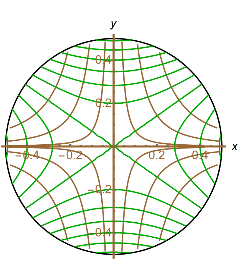
(a) For $\beta_{\bf c}\!=\!\!-0.5$ (interior saddle point of $V$)

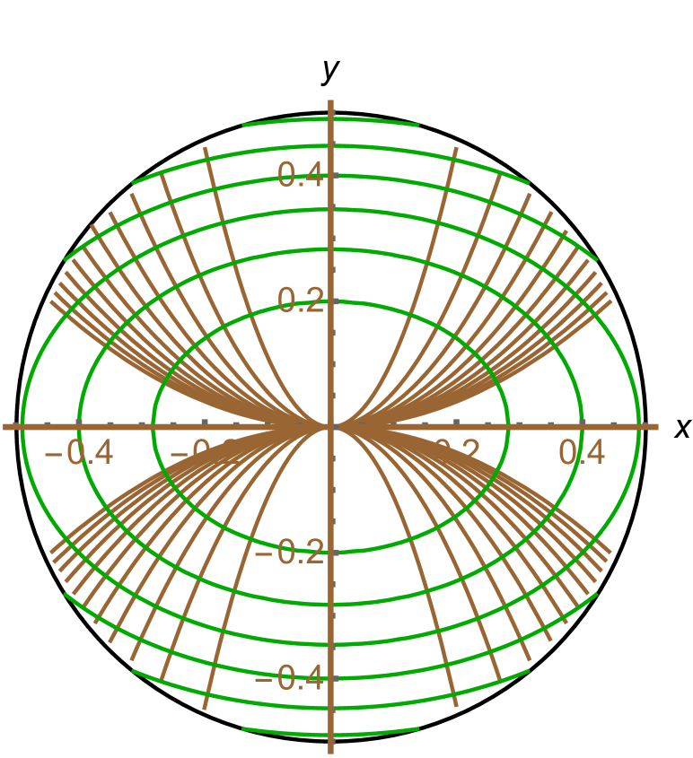
(b) For $\!\beta_{\bf c}\!\!=\!\!0.5$ (interior local extremum of $V$)

Figure 1: Unoriented gradient flow orbits of $V$ (shown in brown) near an interior critical point superposed over the level lines of $V$ (shown in green) for two values of $\beta_{\bf c}$, plotted in principal Cartesian canonical coordinates centered at the critical point. The figure assumes $\omega_{\mathrm{max}}({\bf c})=1/2$, i.e. that the injectivity radius at ${\bf c}$ equals $r({\bf c})=2\operatorname{arctanh}(1/2)=1.098$. The principal coordinate axes correspond to the principal geodesic orbits at ${\bf c}$, which coincide with four special gradient flow orbits.

The scalar potential $\Phi$ of the model can be recovered from the classical effective potential $V=M_{0}\sqrt{2\Phi}$ as:

$$\Phi=\frac{1}{2M_{0}^{2}}V^{2}\approx\frac{{\bar{\lambda}}_{2}({\bf c})^{2}}{2}\left[\bar{V}({\bf c})+\frac{1}{2}\omega^{2}(\beta_{\bf c}\cos^{2}\theta+\sin^{2}\theta)\right]^{2}~{}~{},$$ (38)

where we defined:

$${\bar{\lambda}}_{2}({\bf c})\stackrel{{\scriptstyle{\rm def.}}}{{=}}\frac{\lambda_{2}({\bf c})}{M_{0}}~{}~{},~{}~{}{\bar{V}}({\bf c})\stackrel{{\scriptstyle{\rm def.}}}{{=}}\frac{V({\bf c})}{\lambda_{2}({\bf c})}~{}~{}.$$

Figure 2 shows some numerically computed infrared optimal cosmological curves of the uniformized model parameterized by $(M_{0},\Sigma,G,\Phi)$ near an interior critical point ${\bf c}$. In this figure, we took ${\bar{\lambda}}_{2}({\bf c})=1$, ${\bar{V}}({\bf c})=1$ and $M_{0}=1$, so the rescaled scalar triple $(\Sigma,G_{0},\Phi_{0})$ coincides with $(\Sigma,G,\Phi)$ (recall that the choice of $M_{0}$ does not affect the cosmological or gradient flow orbits). Notice that the accuracy of the first order IR approximation depends on the value of ${\bar{V}}({\bf c})$, since the first IR parameter of ren depends on this value.

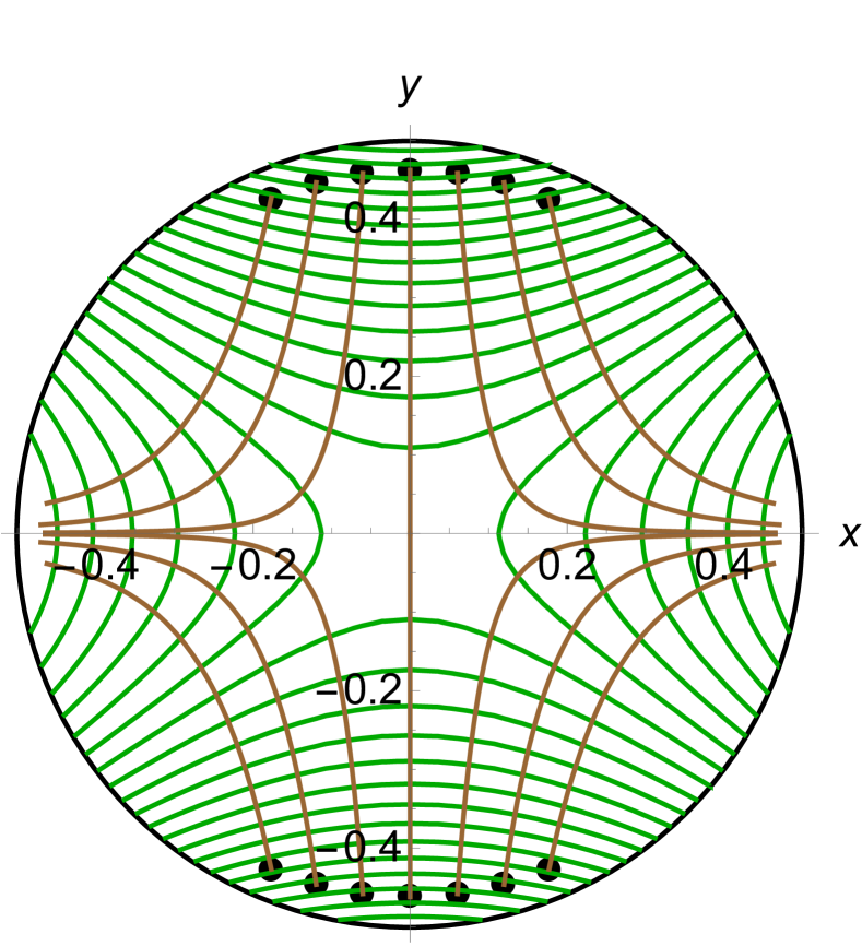
(a) For $\beta_{\bf c}\!=\!\!-0.5$ (interior saddle point of $\Phi$)

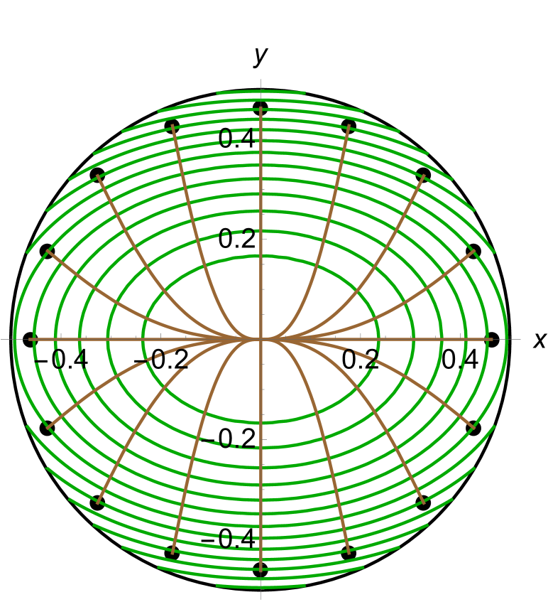
(b) For $\!\beta_{\bf c}\!\!=\!\!0.5$ (interior local extremum of $\Phi$)

Figure 2: Numerically computed orbits of infrared optimal cosmological curves of the uniformized model (shown in brown) near an interior critical point ${\bf c}$, superposed over the level lines of $\Phi$ (shown in green) for two values of $\beta_{\bf c}$. Here $x,y$ are principal Cartesian canonical coordinates centered at the critical point. We assume $\omega_{\mathrm{max}}({\bf c})=1/2$, i.e. that the injectivity radius is $r({\bf c})=2\operatorname{arctanh}(1/2)=1.098$. The figure shows cosmological orbits for IR optimal cosmological curves $\varphi$, whose initial speed belongs to the gradient shell of $(\Sigma,G,V)$. The initial points $\varphi(0)$ of these curves are shown as black dots.

The results above imply the following:

Proposition 3.9.

The asymptotic form of the gradient flow orbits of $(\Sigma,G,V)$ near ${\bf c}$ is determined by the critical modulus $\beta_{\bf c}$, while the orientation of these orbits is determined by the characteristic signs at ${\bf c}$. In particular, the first order IR approximation of those cosmological orbits which have ${\bf c}$ as an $\alpha$- or $\omega$- limit point depends only on these quantities.

Notice that the unoriented orbits of the asymptotic gradient flow near ${\bf c}$ are determined by the positive homothety class of the pair $(\lambda_{1}({\bf c}),\lambda_{2}({\bf c}))$, i.e. by the image of this pair in the quotient $(\mathbb{R}^{\times})^{2}/\mathbb{R}_{>0}$, where the multiplicative group $\mathbb{R}_{>0}$ acts diagonally:

$$(\lambda_{1},\lambda_{2})\rightarrow(\alpha\lambda_{1},\alpha\lambda_{2})~{}~{}\forall\alpha>0~{}~{}.$$

Equivalently, these unoriented orbits depend only on the positive homothety class $[\widehat{\mathrm{Hess}}(V)({\bf c})]\in\mathrm{End}^{s}(T_{\bf c}\Sigma)/\mathbb{R}_{>0}$ of the Hessian operator of $V$ at ${\bf c}$. On the other hand, the topological and smooth topological equivalence class of the gradient flow of $(\Sigma,G,V)$ near ${\bf c}$ is given by the following well-known result (see, for example, (Palis, , Chap. 2, Thm. 5.1)), where $\varepsilon_{1}({\bf c})\stackrel{{\scriptstyle{\rm def.}}}{{=}}\min(\epsilon_{1}({\bf c}),\epsilon_{2}({\bf c}))$ and $\varepsilon_{2}({\bf c})\stackrel{{\scriptstyle{\rm def.}}}{{=}}\max(\epsilon_{1}({\bf c}),\epsilon_{2}({\bf c}))$:

Proposition 3.10.

The gradient flow of $(\Sigma,G,V)$ is locally topologically equivalent near ${\bf c}$ with the gradient flow of the function:

$$V_{0}(x,y)=\frac{1}{2}(\varepsilon_{1}({\bf c})x^{2}+\varepsilon_{2}({\bf c})y^{2})=\left\{\begin{array}[]{ll}\frac{1}{2}(x^{2}+y^{2})&\mbox{if}~{}\mathrm{ind}({\bf c})=0\\ \frac{1}{2}(-x^{2}+y^{2})&\mbox{if}~{}\mathrm{ind}({\bf c})=1\\ -\frac{1}{2}(x^{2}+y^{2})&\mbox{if}~{}\mathrm{ind}({\bf c})=2\end{array}\right.$$

computed with respect to the Euclidean metric:

$$\mathrm{d}s^{2}_{0}=\mathrm{d}x^{2}+\mathrm{d}y^{2}~{}~{}.$$ (39)

This topological equivalence can be chosen to be smooth when $\mathrm{ind}({\bf c})=1$ and when $\mathrm{ind}({\bf c})\in\{0,2\}$ with $\lambda_{1}({\bf c})=\lambda_{2}({\bf c})$. When $\mathrm{ind}({\bf c})\in\{0,2\}$ and $\lambda_{1}({\bf c})\neq\lambda_{2}({\bf c})$, the gradient flow of $(\Sigma,G,V)$ is locally smoothly topologically equivalent near ${\bf c}$ with the gradient flow of the function:

$$V_{0}(x,y)=\frac{1}{2}(\varepsilon_{1}({\bf c})x^{2}+\varepsilon_{2}({\bf c})(2y)^{2})=\left\{\begin{array}[]{ll}\frac{1}{2}(x^{2}+4y^{2})&\mbox{if }~{}\mathrm{ind}({\bf c})=0\\ -\frac{1}{2}(x^{2}+4y^{2})&\mbox{if }~{}\mathrm{ind}({\bf c})=2\end{array}\right.~{}~{}.$$

Hence the IR phase determined by ${\bf c}$ belongs to one of five IR universality classes (in the sense of ren ), which are characterized respectively by the conditions $\mathrm{ind}({\bf c})=1$, $\mathrm{ind}({\bf c})=0$ with $\beta_{\bf c}=1$, $\mathrm{ind}({\bf c})=2$ with $\beta_{\bf c}=1$, $\mathrm{ind}({\bf c})=0$ with $\beta_{\bf c}\neq 1$ and $\mathrm{ind}({\bf c})=2$ with $\beta_{\bf c}\neq 1$. Notice that Proposition 3.9 and equation (36) give detailed information about the asymptotic form of the first order IR orbits of the uniformized model near ${\bf c}$, while Proposition 3.10 characterizes its local IR universality class in the phase determined by ${\bf c}$.

4 The IR phases of noncritical ends

Recall that an end ${\bf e}\in\mathrm{Ends}(\Sigma)$ is noncritical if $(\mathrm{d}\widehat{V})({\bf e})\neq 0$. In this case, the kernel of the linear map $(\mathrm{d}\widehat{V})({\bf e}):T_{\bf e}\widehat{\Sigma}\rightarrow\mathbb{R}$ is one-dimensional and hence we can rotate the Cartesian canonical coordinates $(x,y)$ centered at ${\bf e}$ to ensure that $(\mathrm{d}\widehat{V})({\bf e})$ vanishes on the tangent vector $v_{y}\stackrel{{\scriptstyle{\rm def.}}}{{=}}\frac{\partial}{\partial y}\big{|}_{\bf e}\in T_{\bf e}\widehat{\Sigma}$ and that the quantity $\mu_{\bf e}\stackrel{{\scriptstyle{\rm def.}}}{{=}}(\mathrm{d}\widehat{V})({\bf e})(v_{x})=(\partial_{x}\widehat{V})({\bf e})$ is positive, where $v_{x}\stackrel{{\scriptstyle{\rm def.}}}{{=}}\frac{\partial}{\partial x}\big{|}_{\bf e}$.

Definition 4.1.

A system of special Cartesian canonical coordinates for $(\Sigma,G,V)$ centered at the noncritical end ${\bf e}$ is a system of canonical Cartesian coordinates $(x,y)$ centered at ${\bf e}$ which satisfies the conditions:

$$(\mathrm{d}\widehat{V})({\bf e})(v_{y})=0~{}~{}\mathrm{i.e.}~{}~{}(\partial_{y}\widehat{V})({\bf e})=0~{}~{}$$

and:

$$(\mathrm{d}\widehat{V})({\bf e})(v_{x})>0~{}~{}\mathrm{i.e.}~{}~{}(\partial_{x}\widehat{V})({\bf e})>0~{}~{}.$$

Given such coordinates, we set $\mu_{\bf e}\stackrel{{\scriptstyle{\rm def.}}}{{=}}(\mathrm{d}\widehat{V})({\bf e})(v_{x})=(\partial_{x}\widehat{V})({\bf e})$.

In special Cartesian canonical coordinates centered at a noncritical end ${\bf e}$, the Taylor expansion of the extended potential $\widehat{V}$ at ${\bf e}$ has the form:

$$\widehat{V}(x,y)=\widehat{V}({\bf e})+\mu_{\bf e}x+\mathrm{O}(x^{2}+y^{2})=\widehat{V}({\bf e})+\mu_{\bf e}\omega\cos\theta+\mathrm{O}(\omega^{2})~{}~{}.$$ (40)

In leading order, we have:

$$(\mathrm{grad}_{G}V)^{\omega}=\omega^{4}\partial_{\omega}V=\mu_{\bf e}\omega^{4}\cos\theta$$

$$(\mathrm{grad}_{G}V)^{\theta}=\frac{1}{{\tilde{c}}_{\bf e}}e^{-\frac{2\epsilon_{\bf e}}{\omega}}\partial_{\theta}V=-\frac{\mu_{\bf e}}{{\tilde{c}}_{\bf e}}e^{-\frac{2\epsilon_{\bf e}}{\omega}}\omega\sin\theta~{}~{}.$$ (41)

4.1 Special gradient flow orbits

For $\theta\in\{0,\pi\}$, the gradient flow equation reduces in leading order to $\theta=\mathrm{const}$ and:

$$\frac{\mathrm{d}\omega}{\mathrm{d}q}=\left\{\begin{array}[]{ll}-\mu({\bf e})\omega^{4}&\mbox{if }\theta=0\\ \mu({\bf e})\omega^{4}&\mbox{if }\theta=\pi\end{array}\right.~{}~{},$$

with general solution:

$$\omega=\left\{\begin{array}[]{ll}\frac{1}{(3\mu({\bf e})(q_{0}+q))^{1/3}}&\mbox{if }\theta=0~{}(\mathrm{with}~{}q>-q_{0})\\ \frac{1}{(3\mu({\bf e})(q_{0}-q))^{1/3}}&\mbox{if }\theta=\pi~{}(\mathrm{with}~{}q<q_{0})\end{array}\right.~{}~{},$$

where $q_{0}$ is an arbitrary constant. Shifting $q$ by $q_{0}$ when $\theta=0$ and by $-q_{0}$ when $\theta=\pi$, we can bring this to the form:

$$\omega=\left\{\begin{array}[]{ll}\frac{1}{(3\mu({\bf e})q)^{1/3}}&\mbox{if }\theta=0~{}(\mathrm{with}~{}q>0)\\ \frac{1}{(3\mu({\bf e})|q|)^{1/3}}&\mbox{if }\theta=\pi~{}(\mathrm{with}~{}q<0)\end{array}\right.~{}~{}.$$

This gives two gradient flow orbits which have ${\bf e}$ as a limit point and asymptote close to ${\bf e}$ to the principal geodesic orbits corresponding to the $x$ axis. The first of these lies along the positive $x$ semi-axis ($\theta=0$) and tends to ${\bf e}$ for $q\rightarrow+\infty$ (thus it approximates the late time behavior of a cosmological orbit near the end) while the second lies on the negative $x$ semi-axis ($\theta=\pi$) and tends to ${\bf e}$ for $q\rightarrow-\infty$ (thus it approximates the early time behavior of a cosmological orbit near the end). The cosmological orbit approximated by the gradient orbit with $\theta=0$ flows towards ${\bf e}$ in the distant future while that approximated by the gradient orbit with $\theta=\pi$ originates from ${\bf e}$ in the distant past. Of course, the end ${\bf e}$ is never reached by these orbits since it lies at infinity on $\Sigma$.

4.2 Non-special gradient flow orbits

For $\theta\not\in\{0,\pi\}$, the gradient flow equation reduces to:

$$\frac{\mathrm{d}\omega}{\mathrm{d}\theta}=-\tilde{c}_{\bf e}\omega^{3}\cot(\theta)e^{\frac{2\epsilon_{\bf e}}{\omega}}$$ (42)

with Pfaffian form:

$$\frac{e^{-\frac{2\epsilon_{\bf e}}{\omega}}}{\omega^{3}}\mathrm{d}\omega=-\tilde{c}_{\bf e}\cot(\theta)\mathrm{d}\theta~{}~{}.$$ (43)

Setting $v\stackrel{{\scriptstyle{\rm def.}}}{{=}}\frac{2\epsilon_{\bf e}}{\omega}$, we have:

$$\frac{e^{-\frac{2\epsilon_{\bf e}}{\omega}}}{\omega^{3}}\mathrm{d}\omega=-\frac{1}{4}ve^{-v}\mathrm{d}v=-\frac{1}{4}\mathrm{d}\bm{\gamma}_{2}(v)~{}~{},$$

where:

$$\bm{\gamma}_{n}(v):=\bm{\Gamma}(n,0,v)\stackrel{{\scriptstyle{\rm def.}}}{{=}}\int_{0}^{v}w^{n-1}e^{-w}\mathrm{d}w~{}~{}(\mathrm{with}~{}v\in\mathbb{R})$$ (44)

is the lower incomplete Gamma function of order $n$, which is plotted in Figure 3 for $n=2$. We have:

$$\bm{\gamma}_{2}(v)=1-e^{-v}-ve^{-v}~{}~{}.$$ (45)

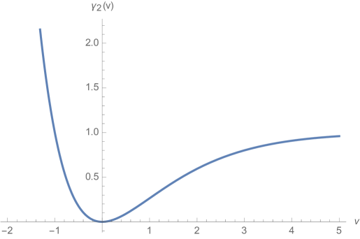
Figure 3: Graph of the incomplete gamma function $\bm{\gamma}_{2}$ of order $2$.

Since $\cot(\theta)\mathrm{d}\theta=\mathrm{d}\log|\sin\theta|$, we find that the non-special gradient flow orbits have the following implicit equation near ${\bf e}$:

$$\frac{1}{4}\bm{\gamma}_{2}\left(\frac{2\epsilon_{\bf e}}{\omega}\right)=A+\tilde{c}_{\bf e}\log|\sin\theta|~{}~{},$$ (46)

where $A$ is an integration constant. In particular, the asymptotic form of the unoriented gradient flow orbits as one approaches the noncritical end ${\bf e}$ is determined in leading order by the constants $\epsilon_{\bf e}$ and ${\tilde{c}}_{\bf e}$. Notice that the asymptotic orbits are independent of the constant $\mu({\bf e})$. Since $\mu({\bf e})>0$, the effective potential increases with $x$ and all curves flow in the direction opposite to that of the $x$ axis.

Asymptotic sectors for non-special gradient flow orbits near the end.

Since the left hand side of (46) is positive while the right hand side is bounded from above by $A$, this equation requires $A>0$. Moreover, a solution exists only for ${\tilde{c}}_{\bf e}\log|\sin\theta|\geq-A$ i.e.:

$$|\sin\theta|>\sigma_{A}:=\sigma_{A}({\bf e})\stackrel{{\scriptstyle{\rm def.}}}{{=}}e^{-\frac{A}{{\tilde{c}}_{\bf e}}}~{}~{},$$

which becomes an equality in the limit $\omega\rightarrow\infty$. Hence each gradient flow curve is contained in the angular region:

$$\theta\in\mathcal{C}_{A}\stackrel{{\scriptstyle{\rm def.}}}{{=}}\left(\theta_{A},\pi-\theta_{A}\right)\cup\left(\pi+\theta_{A},2\pi-\theta_{A}\right)~{}~{},$$ (47)

where:

$$\theta_{A}\stackrel{{\scriptstyle{\rm def.}}}{{=}}\arcsin(\sigma_{A})~{}~{}.$$

When ${\bf e}$ is a flaring end, the left hand side of (46) is smaller than $1/4$, so in this case we have the further condition:

$$|\sin\theta|<\sigma^{\prime}_{A}\stackrel{{\scriptstyle{\rm def.}}}{{=}}e^{\frac{1}{4{\tilde{c}}_{\bf e}}}e^{-\frac{A}{{\tilde{c}}_{\bf e}}}~{}~{}\mathrm{for~{}flaring~{}ends.}$$ (48)

This is automatically satisfied when $A<\frac{1}{4}$, while for $A\geq\frac{1}{4}$ it gives a further constraint which excludes a region of the form $\mathcal{R}_{A}$ but with $\theta_{A}$ replaced by:

$$\theta^{\prime}_{A}\stackrel{{\scriptstyle{\rm def.}}}{{=}}\arcsin(\sigma^{\prime}_{A})~{}~{}.$$

Since $\sigma^{\prime}_{A}>\sigma_{A}$, we have $\theta^{\prime}_{A}>\theta_{A}$, so (47) and (48) give:

$$\theta\in\mathcal{F}_{A}\stackrel{{\scriptstyle{\rm def.}}}{{=}}\left(\theta_{A},\theta^{\prime}_{A}\right)\cup\left(\pi-\theta^{\prime}_{A},\pi-\theta_{A}\right)\cup\left(\pi+\theta_{A},\pi+\theta^{\prime}_{A}\right)\cup\left(2\pi-\theta^{\prime}_{A},2\pi-\theta_{A}\right)~{}~{}.$$

Thus when ${\bf e}$ is a cusp end we have $\theta\in\mathcal{C}_{A}$, while when ${\bf e}$ is a flaring end we have:

$$\theta\in\left\{\begin{array}[]{ll}\mathcal{R}_{A}&\mbox{if }A\in(0,1/4)\\ \mathcal{F}_{A}&\mbox{if }A\in[1/4,\infty)\end{array}\right.~{}~{}.$$

Since the sign $\epsilon_{\bf e}$ is fixed for each end, equation (46) (with fixed $A>0$) produces a single solution $\omega_{A}(\theta)$ for each value of $\theta$ in the allowed region and $\omega_{A}$ is a decreasing and continuous function of $|\sin\theta|$. The right hand side of (46) is invariant under the transformations $\theta\rightarrow\pi-\theta$ and $\theta\rightarrow-\theta$, which correspond to reflections in the coordinate axes. Hence for each $A>0$ we have two gradient flow orbits for a cusp end, while for a flaring end we have two gradient flow orbits when $A\in(0,1/4)$ and four gradient flow orbit when $A\in[1/4,\infty)$. Each orbit is contained in a connected component of the corresponding allowed region. This collection of orbits is invariant under axis reflections.

Non-special gradient flow orbits which have ${\bf e}$ as a limit point.

Distinguish the cases:

1. $\epsilon_{\bf e}=+1$, i.e. ${\bf e}$ is a flaring end. Then (46) becomes:

   $$\frac{1}{4}\bm{\gamma}_{2}\left(\frac{2}{\omega}\right)=A+\tilde{c}_{\bf e}\log|\sin\theta|~{}~{}.$$

   Since the left hand side tends to $\frac{1}{4}$ for $\omega\rightarrow 0$ while the right hand side is bounded from above by $A$, it follows that the gradient flow orbits which reach the end have $A\in[1/4,\infty)$. For each such $A$, we have four gradient flow orbits which reach the end at angles equal to $\pm\theta^{\prime}_{A}\mod\pi$. For $A\rightarrow+\infty$, these orbits asymptote near the origin to the $x$ axis, while for $A\rightarrow 1/4$ they asymptote to the $y$ axis. The orbits obtained for $A\in(0,1/4)$ do not have ${\bf e}$ as a limit point and should be discarded in our approximation.

2. $\epsilon_{\bf e}=-1$, i.e. ${\bf e}$ is a cusp end. Then (46) becomes:

   $$\frac{1}{4}\bm{\gamma}_{2}\left(-\frac{2}{\omega}\right)=A+\frac{1}{(2\pi)^{2}}\log|\sin\theta|\leq A~{}~{}.$$

   In this case, the left hand side tends to infinity when $\omega$ tends to zero so a gradient flow orbit cannot have ${\bf e}$ as a limit point because $A$ is finite. When $A$ tends to infinity, the gradient flow orbits approach the noncritical cusp closer and closer but they never pass through it. Along the two gradient flow orbits with integration constant $A$, the smallest value $\omega_{0}:=\omega_{0}(A)$ of $\omega$ is realized for $\theta=\frac{\pi}{2}$ or $\theta=\frac{3\pi}{2}$ (at the points where these orbits intersect the $y$ axis) and is the solution of the equation:

   $$\frac{1}{4}\bm{\gamma}_{2}\left(-\frac{2}{\omega_{0}}\right)=A~{}~{}.$$

Figure 4 shows some unoriented asymptotic gradient flow orbits close to each type of noncritical end.

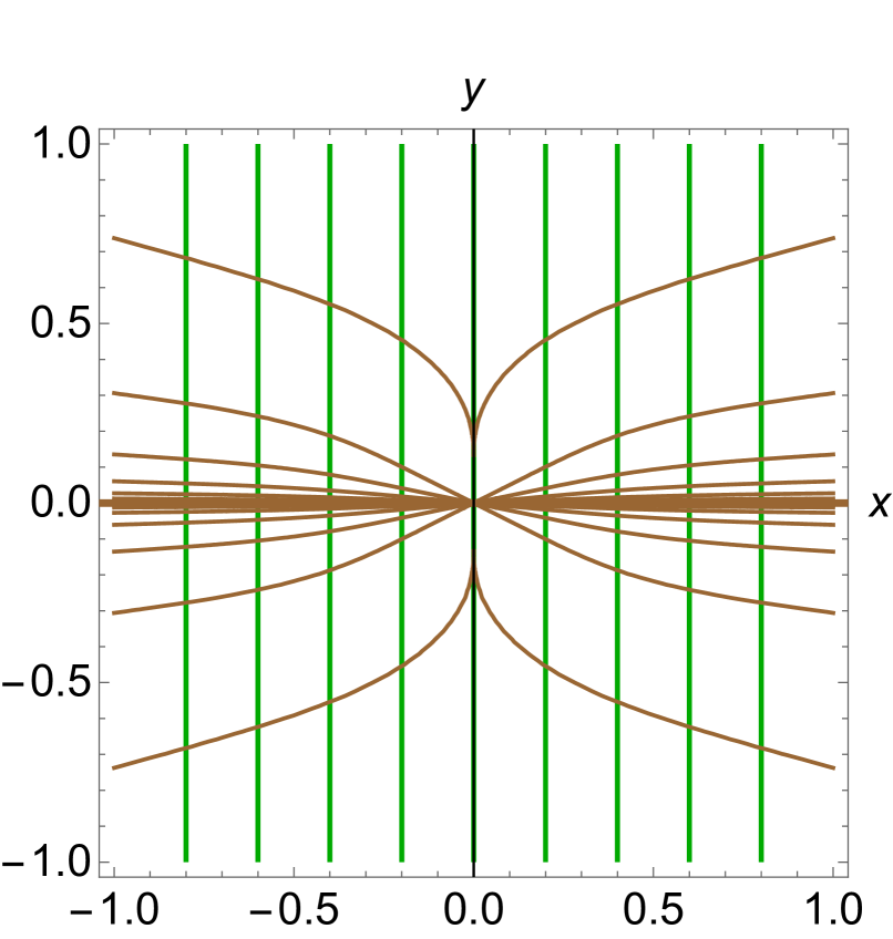
(a) Plane end.

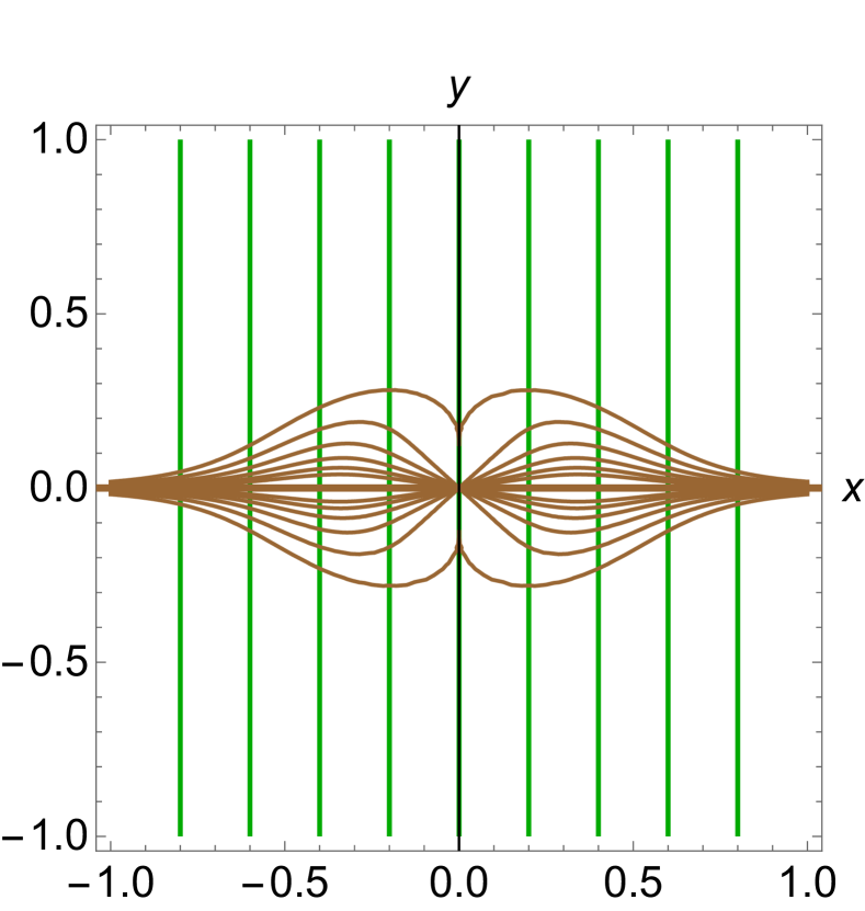
(b) Horn end.

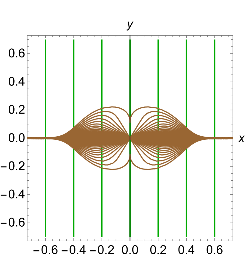
(c) Funnel end with $\ell=1$.

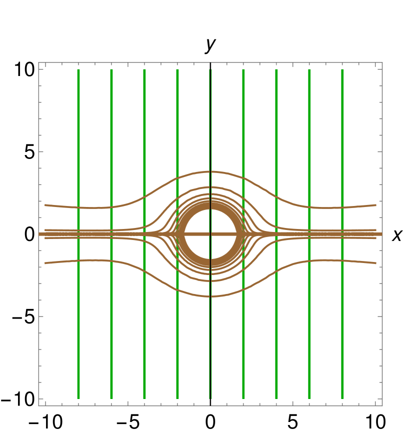
(d) Cusp end.

Figure 4: Unoriented gradient flow orbits of $V$ (shown in brown) and level sets of $V$ (shown in green) near noncritical plane, horn, funnel and cusp ends in special Cartesian canonical coordinates centered at the end. For the funnel end we took $\ell=1$. For flaring ends, we show only orbits which have the end as a limit point (which correspond to $A\geq 1/4$. The orbits flow from right to left since $\mu_{\bf e}>0$.

The extended scalar potential ${\hat{\Phi}}$ of the canonical model can be recovered from the extended classical effective potential as:

$${\hat{\Phi}}=\frac{1}{2M_{0}^{2}}\widehat{V}^{2}\approx\frac{1}{2}{\bar{\mu}}_{\bf e}^{2}\left[\hat{\bar{V}}({\bf e})+\omega\cos\theta\right]^{2}~{}~{},$$ (49)

where we defined:

$${\bar{\mu}}_{\bf e}\stackrel{{\scriptstyle{\rm def.}}}{{=}}\frac{\mu_{\bf e}}{M_{0}}~{}~{},~{}~{}{\hat{\bar{V}}}({\bf e})\stackrel{{\scriptstyle{\rm def.}}}{{=}}\frac{{\hat{V}}({\bf e})}{\mu_{\bf e}}~{}~{}.$$

Figure 5 shows some infrared optimal cosmological orbits of the uniformized model parameterized by $(M_{0},\Sigma,G,\Phi)$ near noncritical ends ${\bf e}$; the initial point of each orbit is shown as a black dot. In this figure, we took ${\bar{\mu}}_{\bf e}=1$, ${\hat{\bar{V}}}({\bf e})=1$ and $M_{0}=1$. Notice that the accuracy of the first order IR approximation depends on the value of ${\hat{\bar{V}}}({\bf e})$, since the first IR parameter of ren depends on this value.

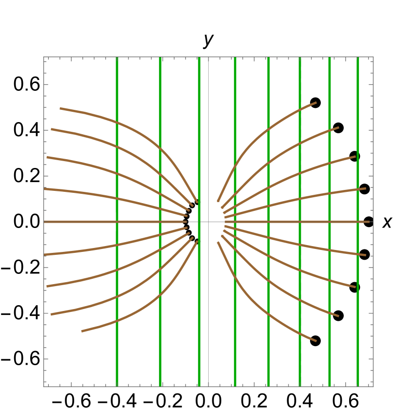
(a) Plane end.

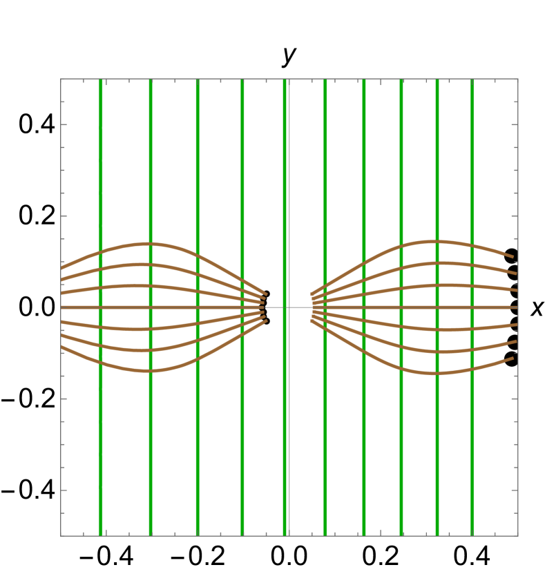
(b) Horn end.

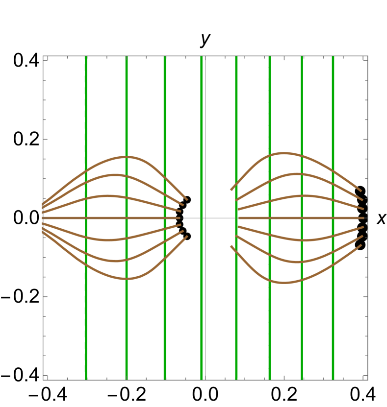
(c) Funnel end with $\ell=1$.

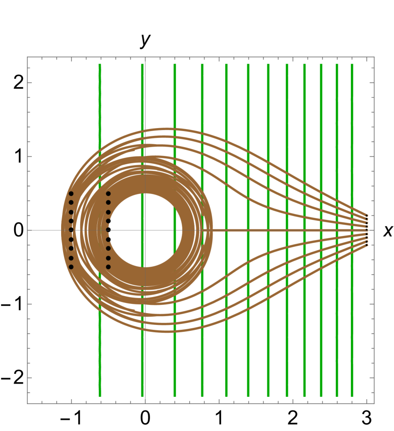
(d) Cusp end.

Figure 5: Numerically computed infrared optimal cosmological orbits (shown in brown) and level sets of $\Phi$ (shown in green) near noncritical plane, horn, funnel and cusp ends in special Cartesian canonical coordinates centered at the end. For the funnel end we took $\ell=1$. The initial values of the corresponding curves are shown as black dots, while the initial speeds lie in the gradient shell of $(\Sigma,G,V)$.

The case of noncritical cusp ends is particularly interesting. For clarity, Figure 6 shows the evolution of a few infrared optimal cosmological curves for four consecutive cosmological times.

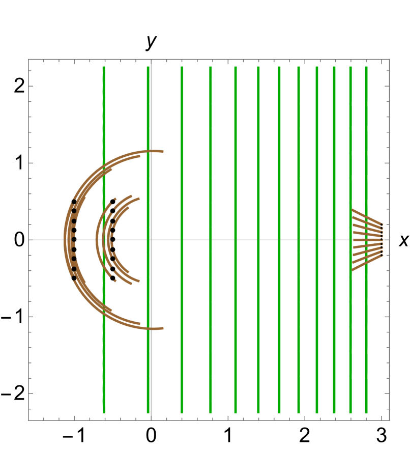
(a) For $t=0.01$.

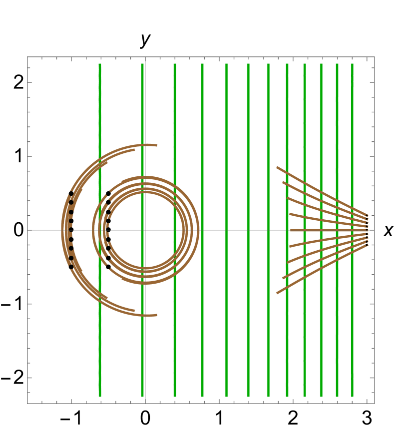
(b) For $t=0.04$.

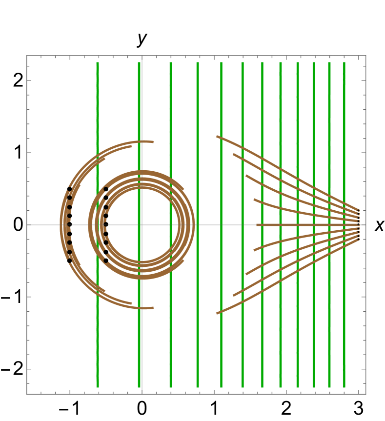
(c) For $t=0.07$.

(d) For $t=0.3$.

Figure 6: Numerically computed infrared optimal cosmological orbits of the canonical model (shown in brown) and level sets of $\Phi$ (shown in green) near a noncritical cusp end, with initial points shown as black dots and initial speeds taken in the gradient flow shell of $(\Sigma,G,V)$. The four figures show the orbits for cosmological times between zero and $t=0.01$, $0.04$, $0.07$ and $0.3$ respectively.

4.3 Stable and unstable manifolds of noncritical ends under the effective gradient flow

The discussion above shows that noncritical flaring ends behave like fictitious stationary points of the gradient flow of $(\Sigma,G,V)$ even though Freudenthal ends are not points of $\Sigma$ and even though $\widehat{V}$ does not have a critical point at a non-critical end. The stable and unstable manifolds of such an end (see (9)) are connected and of dimension two:

$$\dim\mathcal{S}({\bf e})=\dim\mathcal{U}({\bf e})=2~{}~{}\mathrm{for}~{}~{}{\bf e}=\mathrm{noncritical~{}flaring~{}end}~{}~{},$$

a dimension count which differs from that of ordinary hyperbolic fixed points of dynamical systems. On the other hand, noncritical cusp ends do not behave like stationary points of the effective gradient flow; instead, they “repel” all gradient flow orbits with the exception of the two special orbits which lie on the $x$ axis and hence correspond to geodesic orbits having the cusp as a limit point. These special orbits form the stable and unstable manifolds of a noncritical cusp end, which are connected and one-dimensional:

$$\dim\mathcal{S}({\bf e})=\dim\mathcal{U}({\bf e})=1~{}~{}\mathrm{for}~{}~{}{\bf e}=\mathrm{noncritical~{}cusp~{}end}~{}~{}.$$

With the exception of the two special orbits, every other effective gradient flow orbit never reaches the noncritical cusp end. Notice that the noncritical ends do not act as attractors of the effective gradient flow.

5 The IR phases of critical ends

Consider principal Cartesian canonical coordinates $(x,y)$ centered at a critical end ${\bf e}$ (see Subsection 2.8). In such coordinates, we have:

$$(\mathrm{grad}V)^{\omega}\approx\omega^{4}\partial_{\omega}V\approx\omega^{5}\left[\lambda_{1}({\bf e})\cos^{2}\theta+\lambda_{2}({\bf e})\sin^{2}\theta\right]$$ (50)

$$(\mathrm{grad}V)^{\theta}\approx\frac{1}{f_{\bf e}(1/\omega)}\partial_{\theta}V\approx\frac{\lambda_{2}({\bf e})-\lambda_{1}({\bf e})}{{\tilde{c}}_{\bf e}}\omega^{2}e^{-\frac{2\epsilon_{\bf e}}{\omega}}\sin\theta\cos\theta~{}~{}.$$

5.1 Special gradient flow orbits

For $\theta\in\{0,\frac{\pi}{2},\pi,\frac{3\pi}{2}\}$, the gradient flow equation of $(\Sigma,G,V)$ reduces in leading order near ${\bf e}$ to $\theta=\mathrm{const}$ and:

$$\frac{\mathrm{d}\omega}{\mathrm{d}q}=\left\{\begin{array}[]{ll}\lambda_{1}({\bf e})\omega^{5}&\mbox{if }\theta\in\{0,\pi\}\\ \lambda_{2}({\bf e})\omega^{5}&\mbox{if }\theta\in\{\frac{\pi}{2},\frac{3\pi}{2}\}\end{array}\right.~{}~{},$$

with general solution:

$$\omega=\left\{\begin{array}[]{ll}\frac{1}{[4\lambda_{1}({\bf e})(q_{0}-q)]^{1/4}}&\mbox{if }\theta\in\{0,\pi\}~{}(\mathrm{with}~{}q<q_{0})\\ \frac{1}{[4\lambda_{2}({\bf e})(q_{0}-q)]^{1/4}}&\mbox{if }\theta\in\{\frac{\pi}{2},\frac{3\pi}{2}\}~{}(\mathrm{with}~{}q<q_{0})\end{array}\right.~{}~{}.$$

Shifting $q$ by $q_{0}$ brings this to the form:

$$\omega=\left\{\begin{array}[]{ll}\frac{1}{[4\lambda_{1}({\bf e})|q|]^{1/4}}&\mbox{if }\theta\in\{0,\pi\}~{}(\mathrm{with}~{}q<0)\\ \frac{1}{[4\lambda_{2}({\bf e})|q|]^{1/4}}&\mbox{if }\theta\in\{\frac{\pi}{2},\frac{3\pi}{2}\}~{}(\mathrm{with}~{}q<0)\end{array}\right.~{}~{}.$$

This gives four gradient flow orbits which tend to ${\bf e}$ for $q\rightarrow-\infty$ and asymptote to the principal geodesic orbits near ${\bf e}$.

5.2 Non-special gradient flow orbits

For $\theta\not\in\{0,\frac{\pi}{2},\pi,\frac{3\pi}{2}\}$, the gradient flow equation reduces to:

$$\frac{\mathrm{d}\omega}{\mathrm{d}\theta}=\frac{{\tilde{c}}_{\bf e}}{\lambda_{2}({\bf e})-\lambda_{1}({\bf e})}\omega^{3}e^{\frac{2\epsilon_{\bf e}}{\omega}}\left[\lambda_{1}({\bf e})\cot\theta+\lambda_{2}({\bf e})\tan\theta\right]~{}~{},$$

which can be written as:

$$[\lambda_{2}({\bf e})-\lambda_{1}({\bf e})]\omega^{-3}e^{-\frac{2\epsilon_{\bf e}}{\omega}}\mathrm{d}\omega={\tilde{c}}_{\bf e}\left[\lambda_{1}({\bf e})\cot\theta+\lambda_{2}({\bf e})\tan\theta\right]\mathrm{d}\theta~{}~{}.$$ (51)

Setting $v\stackrel{{\scriptstyle{\rm def.}}}{{=}}\frac{2\epsilon_{\bf e}}{\omega}$ brings (51) to the form:

$$\frac{1}{4}[\lambda_{1}({\bf e})-\lambda_{2}({\bf e})]ve^{-v}\mathrm{d}v={\tilde{c}}_{\bf e}\left[\lambda_{1}({\bf e})\cot\theta+\lambda_{2}({\bf e})\tan\theta\right]\mathrm{d}\theta~{}~{}.$$ (52)

We have $ve^{-v}\mathrm{d}v=\mathrm{d}\bm{\gamma}_{2}(v)$, where $\bm{\gamma}_{2}(v)$ is the lower incomplete Gamma function of order $2$ (see (44)). Hence (52) gives the following implicit equation for the asymptotic gradient flow orbits near a critical end ${\bf e}$:

$$\frac{1}{4}[\lambda_{1}({\bf e})-\lambda_{2}({\bf e})]\bm{\gamma}_{2}\left(\frac{2\epsilon_{\bf e}}{\omega}\right)=A+{\tilde{c}}_{\bf e}\left[\,\lambda_{1}({\bf e})\log|\sin\theta|-\lambda_{2}({\bf e})\log|\cos\theta|\,\right]~{}~{},$$ (53)

where $A$ is an integration constant. Since:

$$\bm{\gamma}_{2}(v)=1-e^{-v}-ve^{-v}~{}~{},$$

this can be written explicitly as:

$$\frac{1}{4}[\lambda_{1}({\bf e})-\lambda_{2}({\bf e})]\left[1-e^{-\frac{2\epsilon_{\bf e}}{\omega}}-\frac{2\epsilon_{\bf e}}{\omega}e^{-\frac{2\epsilon_{\bf e}}{\omega}}\right]=A+{\tilde{c}}_{\bf e}\left[\,\lambda_{1}({\bf e})\log|\sin\theta|-\lambda_{2}({\bf e})\log|\cos\theta|\,\right]~{}~{}.$$ (54)

Distinguish the cases:

1. $V$ is circular at ${\bf e}$, i.e. $\lambda_{1}({\bf e})=\lambda_{2}({\bf e}):=\lambda({\bf e})$ (which amounts to $\beta_{\bf e}=1$). Then (53) becomes:

   $$\log|\sin\theta|-\log|\cos\theta|=B~{}~{}\mathrm{i.e.}~{}~{}\tan\theta=\pm e^{B}\Longleftrightarrow\theta=\pm\arctan(e^{B})\!\!\!\mod\pi$$ (55)

   with $B\stackrel{{\scriptstyle{\rm def.}}}{{=}}-\frac{A}{\lambda({\bf e}){\tilde{c}}_{\bf e}}$ and hence $\theta$ is constant for all asymptotic gradient flow curves. In this case, the asymptotic gradient flow orbits near ${\bf e}$ are geodesic orbits of $(\Sigma,G)$ having ${\bf e}$ as a limit point. For each value of $B$, there are exactly four such orbits.

2. $V$ is not circular at ${\bf e}$, i.e. $\beta_{\bf e}\neq 1$. Then (53) can be written as:

   $$\bm{\gamma}_{2}\left(\frac{2\epsilon_{\bf e}}{\omega}\right)=1-e^{-\frac{2\epsilon_{\bf e}}{\omega}}-\frac{2\epsilon_{\bf e}}{\omega}e^{-\frac{2\epsilon_{\bf e}}{\omega}}=C-\frac{4{\tilde{c}}_{\bf e}}{1-\beta_{\bf e}}\left(\beta_{\bf e}\log|\sin\theta|-\log|\cos\theta|\right)~{}~{},$$ (56)

   where $C\stackrel{{\scriptstyle{\rm def.}}}{{=}}\frac{4A}{\lambda_{1}({\bf e})-\lambda_{2}({\bf e})}$.

Thus:

Proposition 5.1.

The unoriented orbits of the asymptotic gradient flow of $(\Sigma,G,V)$ near a critical end ${\bf e}$ are determined by the hyperbolic type of the end (i.e. by $\epsilon_{\bf e}$ and ${\tilde{c}}_{\bf e}$) and by the critical modulus $\beta_{\bf e}$, while the orientation of the orbits is determined by the critical signs $\epsilon_{i}({\bf e})$, which satisfy $\epsilon_{1}({\bf e})\epsilon_{2}({\bf e})=1$.

Asymptotic sectors for non-special gradient flow curves when $\lambda_{1}({\bf e})\neq\lambda_{2}({\bf e})$.

Let us assume that $\lambda_{1}({\bf e})\neq\lambda_{2}({\bf e})$ i.e. that $\beta_{\bf e}<1$. Then (56) reads:

$$\bm{\gamma}_{2}\left(\frac{2\epsilon_{\bf e}}{\omega}\right)=C-\frac{4{\tilde{c}}_{\bf e}}{1-\beta_{\bf e}}H(\theta;\beta_{\bf e})~{}~{},$$ (57)

where $H:\mathrm{S}^{1}\times[-1,1)\rightarrow\overline{\mathbb{R}}$ is the function defined through:

$$H(\theta;\beta)\stackrel{{\scriptstyle{\rm def.}}}{{=}}\beta\log|\sin\theta|-\log|\cos\theta|~{}~{}.$$

This function satisfies:

$$H(-\theta,\beta)=H(\pi-\theta;\beta)=H(\theta,\beta)~{}~{}.$$

Notice that:

$$\bm{\gamma}_{2}(v)\in\left\{\begin{array}[]{ll}(0,1)&\mbox{if }~{}v>0\\ (0,+\infty)&\mbox{if }~{}v<0\end{array}\right.$$

and:

$$\bm{\gamma}_{2}(-\infty)=+\infty~{}~{},~{}~{}\bm{\gamma}_{2}(0)=0~{}~{},~{}~{}\bm{\gamma}_{2}(+\infty)=1~{}~{}.$$

Moreover:

$$\bm{\gamma}_{2}^{\prime}(v)=ve^{-v}\left\{\begin{array}[]{ll}>0&\mbox{if}~{}v>0\\ =0&\mbox{if}~{}v=0\\ <0&\mbox{if}~{}v<0\end{array}\right.~{}~{},$$

hence $\bm{\gamma}_{2}(v)$ is strictly decreasing for $v<0$ and strictly increasing for $v>0$. Since $\omega>0$, we have:

$$v:=\frac{2\epsilon_{\bf e}}{\omega}\in\left\{\begin{array}[]{ll}>0&\mbox{if }~{}{\bf e}=\mathrm{flaring~{}end}\\ <0&\mbox{if }~{}{\bf e}=\mathrm{cusp~{}end}\end{array}\right.~{}~{},$$

which gives:

$$\bm{\gamma}_{2}\left(\frac{2\epsilon_{\bf e}}{\omega}\right)\in\left\{\begin{array}[]{ll}(0,1)&\mbox{if }~{}{\bf e}=\mathrm{flaring~{}end}\\ (0,+\infty)&\mbox{if }~{}{\bf e}=\mathrm{cusp~{}end}\end{array}\right.~{}~{}.$$ (58)

Hence (57) requires:

$$C-\frac{4{\tilde{c}}_{\bf e}}{1-\beta_{\bf e}}H(\theta;\beta_{\bf e})\in\left\{\begin{array}[]{ll}(0,1)&\mbox{if }~{}{\bf e}=\mathrm{flaring~{}end}\\ (0,+\infty)&\mbox{if }~{}{\bf e}=\mathrm{cusp~{}end}\end{array}\right.~{}~{}.$$ (59)

Since $H(\theta;\beta)$ tends to $\pm\infty$ for $\theta\,\mathrm{mod}\,2\pi\in\{0,\frac{\pi}{2},\pi,\frac{3\pi}{2}\}$, these values of $\theta$ cannot be attained along any asymptotic gradient flow orbit. Hence all such orbits are contained in the complement of the principal coordinate axes in the $(x,y)$-plane, which means that they cannot meet the principal geodesic orbits close to the end ${\bf e}$. For fixed $\beta$, the function $H(\theta,\beta)$ is invariant under the action of the Klein four-group $\mathbb{Z}_{2}\times\mathbb{Z}_{2}$ generated by the reflections $\theta\rightarrow-\theta$ and $\theta\rightarrow\pi-\theta$ with respect to the $x$ and $y$ axes; in particular, this function is periodic of period $\pi$ and its restriction to the interval $(0,\pi)$ is symmetric with respect to $\frac{\pi}{2}$, hence it suffices to study the restriction of $H$ to the interval $\theta\in(0,\frac{\pi}{2})$. Noticing that:

$$\lim_{\theta\rightarrow 0}H(\theta,\beta)=-\mathrm{sign}(\beta)\infty~{}~{},~{}~{}\lim_{\theta\rightarrow\frac{\pi}{2}}H(\theta,\beta)=+\infty$$

we distinguish the cases:

1. $\beta\in[-1,0)$. For $\theta\in(0,\pi/2)$, we have:

   $$\frac{\mathrm{d}H(\theta;\beta)}{\mathrm{d}\theta}=\beta\cot\theta+\tan\theta\left\{\begin{array}[]{ll}<0&\mbox{if}~{}~{}0\leq\theta<\theta_{0}(\beta)\\ =0&\mbox{if}~{}~{}\theta=\theta_{0}(\beta)\\ >0&\mbox{if}~{}~{}\theta_{0}(\beta)\leq\theta\leq\frac{\pi}{2}\end{array}\right.~{}~{},$$

   where $\theta_{0}(\beta)\stackrel{{\scriptstyle{\rm def.}}}{{=}}\arctan\sqrt{|\beta|}$. In this case, $H(\theta;\beta)$ tends to $+\infty$ at the endpoints of the interval $(0,\frac{\pi}{2})$ and attains its minimum within this interval at the point $\theta_{0}(\beta)$, the minimum value being given by:

   $$\mu(\beta)\stackrel{{\scriptstyle{\rm def.}}}{{=}}H(\theta_{0}(\beta),\beta)=\frac{1}{2}\Big{[}(1+|\beta|)\log(1+|\beta|)-|\beta|\log|\beta|\Big{]}~{}~{}.$$

   Notice that $\mu$ is an increasing function of $|\beta|$ (hence a decreasing function of $\beta$) and that we have:

   $$\mu(\beta)\in(0,\log 2]~{}~{}\mathrm{with}~{}~{}\mu(-1)=\log 2~{}~{},~{}~{}\mu(0^{-})=0~{}~{}.$$

   It follows that $H(\theta,\beta)$ tends to $+\infty$ for $\theta\!\in\!\{0,\frac{\pi}{2},\pi,\frac{3\pi}{2}\}$ and attains its minimum $\mu(\beta)$ on $\mathrm{S}^{1}$ for $\theta\in\{\theta_{0}(\beta),\pi-\theta_{0}(\beta),\theta_{0}(\beta)+\pi,2\pi-\theta_{0}(\beta)\}$ (see Figure 7).

   
   

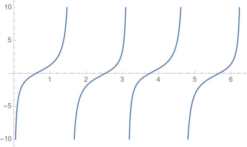
   (a) $\frac{\mathrm{d}H(\theta;\beta)}{\mathrm{d}\theta}$ for $\beta=-1/2$ and $\theta\in(0,2\pi)$.

   

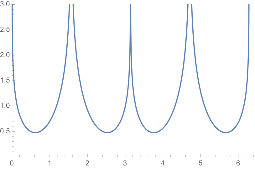
   (b) $H(\theta;\beta)$ for $\beta=-1/2$ and $\theta\in(0,2\pi)$.

   Figure 7: Plots of $\frac{\mathrm{d}H(\theta;\beta)}{\mathrm{d}\theta}$ and $H(\theta;\beta)$ for $\beta=-1/2$ and $\theta\in(0,2\pi)$.

2. $\beta\in(0,1)$. Then the derivative:

   $$\frac{\mathrm{d}H(\theta;\beta)}{\mathrm{d}\theta}=\left(\beta+\tan^{2}\theta\right)\cot\theta$$

   is strictly positive for $\theta\in(0,\frac{\pi}{2})\cup(\pi,\frac{3\pi}{2})$ and strictly negative for $\theta\in(\frac{\pi}{2},\pi)\cup(\frac{3\pi}{2},2\pi)$. Hence $H(\theta,\beta)$ increases strictly from $-\infty$ to $+\infty$ along the $\theta$-intervals $(0,\frac{\pi}{2})$ and $(\pi,\frac{3\pi}{2})$ and decreases strictly from $+\infty$ to $-\infty$ along the $\theta$-intervals $(\frac{\pi}{2},\pi)$ and $(\frac{3\pi}{2},2\pi)$. Thus $H$ tends to $-\infty$ for $\theta\in\{0,\pi\}$ and to $+\infty$ for $\theta\in\{\frac{\pi}{2},\frac{3\pi}{2}\}$ and is strictly monotonous on the circle intervals separating these four special points of $\mathrm{S}^{1}$ (see Figure 8).

   

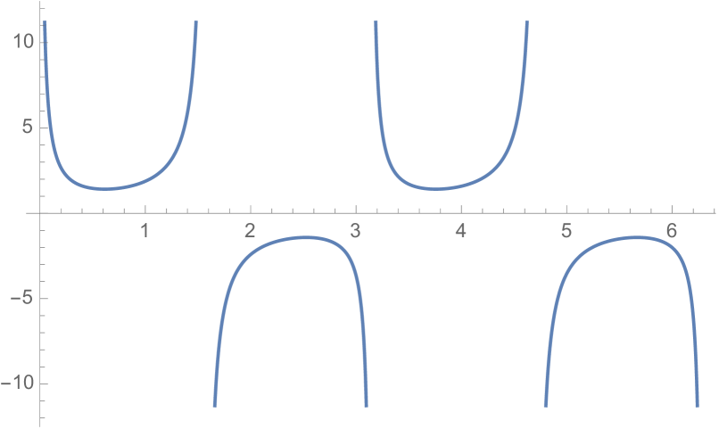
   (a) $\frac{\mathrm{d}H(\theta;\beta)}{\mathrm{d}\theta}$ for $\beta=1/2$ and $\theta\in(0,2\pi)$.

   

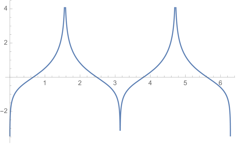
   (b) $H(\theta;\beta)$ for $\beta=1/2$ and $\theta\in(0,2\pi)$.

   Figure 8: Plots of $\frac{\mathrm{d}H(\theta;\beta)}{\mathrm{d}\theta}$ and $H(\theta;\beta)$ for $\beta=1/2$ and $\theta\in(0,2\pi)$.

Returning to condition (59), we distinguish the cases:

1. ${\bf e}$ is a flaring end. Then (59) requires $C-\frac{4{\tilde{c}}_{\bf e}}{1-\beta_{\bf e}}H(\theta;\beta_{\bf e})\in(0,1)$. We have two sub-cases:

   1. $\beta_{\bf e}\in[-1,0)$. Then $H(\theta,\beta_{\bf e})\geq\mu(\beta_{\bf e})$ and $C$ is constrained by the condition:

      $$C>\frac{4{\tilde{c}}_{\bf e}}{1-\beta_{\bf e}}\mu(\beta_{\bf e})~{}~{}.$$ (60)

      Each gradient flow orbit corresponds to a fixed value of $C$. On any such orbit, condition (59) gives:

      $$\frac{4{\tilde{c}}_{\bf e}}{1-\beta_{\bf e}}H(\theta;\beta_{\bf e})\in(C-1,C)~{}~{}.$$ (61)

      We have two possibilities:

      • When $C-1\geq\frac{4{\tilde{c}}_{\bf e}}{1-\beta_{\bf e}}\mu(\beta_{\bf e})$, condition (61) constrains $\theta$ to lie in a union of eight disjoint open intervals on $\mathrm{S}^{1}$. These eight intervals divide into four successive pairs, where both intervals of each pair are contained in one of the four quadrants and the four pairs are related by the action of $\mathbb{Z}_{2}\times\mathbb{Z}_{2}$. Hence for each fixed value of $C$ we have eight orbits in the $(x,y)$ plane, which arrange into four pairs lying in the four quadrants; the pairs are related to each other by the action of $\mathbb{Z}_{2}\times\mathbb{Z}_{2}$. We will see below that these eight orbits have ${\bf e}$ as a limit point.

      • When $C-1<\frac{4{\tilde{c}}_{\bf e}}{1-\beta_{\bf e}}\mu(\beta_{\bf e})$, the condition above constrains $\theta$ to lie in a union of four disjoint open intervals on $\mathrm{S}^{1}$ (each lying in a different quadrant) which is invariant under the action of $\mathbb{Z}_{2}\times\mathbb{Z}_{2}$. In this case, we have four orbits (one in each quadrant) which are related by this action. These orbits do not have ${\bf e}$ as a limit point (see below).

   2. $\beta_{\bf e}\in(0,1)$. Then $C$ is unconstrained since $H(\theta,\beta)$ is not bounded from below or from above. On any gradient flow orbit corresponding to $C$, condition (61) must be satisfied. This constrains $\theta$ to lie in a union of four disjoint open circular intervals which is invariant under the action of the Klein four-group on $\mathrm{S}^{1}$. Hence for each $C$ we have four gradient flow orbits (one in each quadrant) which are related by the action of $\mathbb{Z}_{2}\times\mathbb{Z}_{2}$. These four orbits have ${\bf e}$ as a limit point (see below).

2. ${\bf e}$ is a cusp end. In this case, condition (59) requires $\frac{4{\tilde{c}}_{\bf e}}{1-\beta_{\bf e}}H(\theta;\beta_{\bf e})<C$. We have two sub-cases:

   1. $\beta_{\bf e}\in[-1,0)$. In this case, we must have $C>\frac{4{\tilde{c}}_{\bf e}}{1-\beta_{\bf e}}\mu(\beta_{\bf e})$ and $\theta$ lies in a union of four disjoint open intervals on $\mathrm{S}^{1}$ which is invariant under the action of $\mathbb{Z}_{2}\times\mathbb{Z}_{2}$. Hence for each value of $C$ we have four gradient flow orbits (each in one of the four quadrants) which are related by the action of $\mathbb{Z}_{2}\times\mathbb{Z}_{2}$. We will see below that these orbits do not have ${\bf e}$ as a limit point.

   2. $\beta_{\bf e}\in(0,1)$. In this case, $C$ is unconstrained and (since the values $\theta=0,\pi$ are forbidden) $\theta$ lies in a union of four disjoint open intervals on $\mathrm{S}^{1}$ of the form $(0,\theta_{0})\cup(\pi-\theta_{0},\pi)\cup(\pi+\theta_{0},2\pi-\theta_{0})$. Hence for each value of $C$ we have four gradient flow orbits (one in each quadrant), which are related to each other by reflections in the coordinate axes. These orbits have ${\bf e}$ as a limit point.

Non-special gradient flow orbits having ${\bf e}$ as a limit point.

Suppose that $\beta_{\bf e}\neq 1$ and distinguish the cases:

1. ${\bf e}$ is a flaring end. In this case, we have $\epsilon_{\bf e}=+1$ and the left hand side of (56) tends to $1$ as $\omega\rightarrow 0$. In this limit, the equation reduces to:

   $$H(\theta,\beta_{\bf e})=\frac{C-1}{{4{\tilde{c}}_{\bf e}}}(1-\beta_{\bf e})~{}~{}.$$ (62)

   Distinguish the cases:

   • When $\beta_{\bf e}\in[-1,0)$, condition (62) requires $C\geq 1+\frac{4{\tilde{c}}_{\bf e}}{1-\beta_{\bf e}}\mu(\beta_{\bf e})$. When this inequality holds strictly, the condition has eight solutions of the form $\theta=\pm\theta_{1}\mod\pi$ and $\theta=\pm\theta_{2}\mod\pi$, where $\theta_{1}$ and $\theta_{2}$ are the two solutions lying in the interval $[0,\frac{\pi}{2})$ (see Figure 7(b)). The corresponding eight gradient flow orbits asymptote to the end making one of these angles with the $x$ axis. The angles $\theta_{1}$ and $\theta_{2}$ coincide when $C=1+\frac{4{\tilde{c}}_{\bf e}}{1-\beta_{\bf e}}\mu(\beta_{\bf e})$; in this case, the geodesics lying in the same quadrant reach the end at the same angle.

   • When $\beta_{\bf e}\in(0,1)$, condition (62) does not constrain $C$. This condition has four solutions of the form $\theta=\pm\theta_{0}\mod\pi$, where $\theta_{0}$ is the solution lying in the interval $[0,\frac{\pi}{2})$ (see Figure 8(b)). The corresponding four gradient flow orbits reach the origin making these angles with the $x$ axis.

2. ${\bf e}$ is a cusp end. In this case, we have $\epsilon_{\bf e}=-1$ and the left hand side of (56) tends to plus infinity when $\omega\rightarrow 0$. This requires that the right hand side also tends to $+\infty$, which (for fixed $C$) happens when $H(\theta,\beta_{\bf e})$ tends to $-\infty$. Hence we must have $\beta_{\bf e}>0$ and $\theta\rightarrow 0$ or $\theta\rightarrow\pi$, which means that each of the four gradient flow orbits which asymptote near the end to one of the two principal geodesic orbits which have ${\bf e}$ as a limit point and correspond to the semi-axes determined by the $x$ axis.

A few unoriented gradient flow orbits of the effective scalar triple $(\Sigma,G,V)$ near critical ends are plotted in Figures 9-12 in principal canonical coordinates centered at the end.

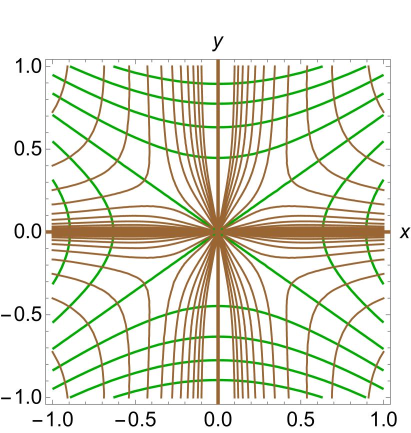
(a) For $\beta_{\bf e}=-1/2$

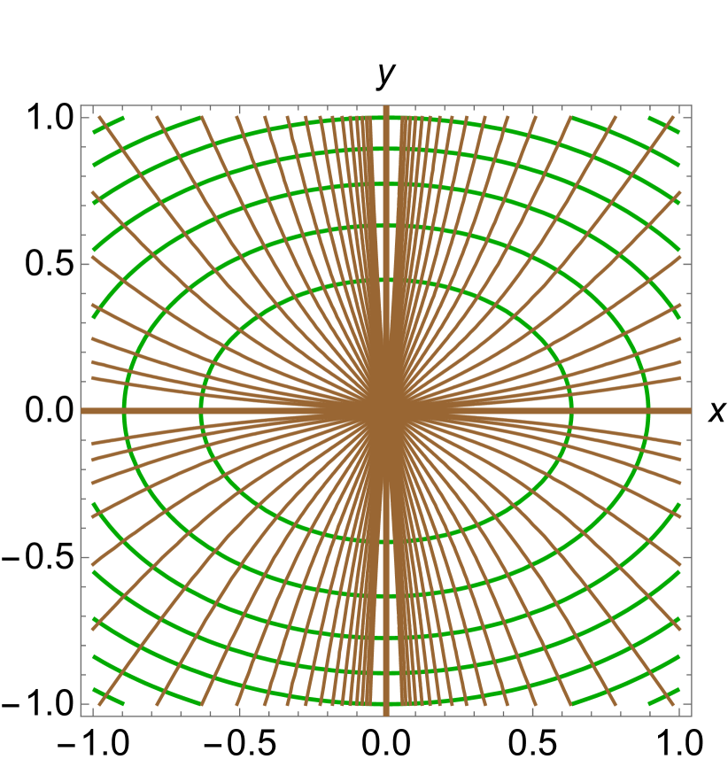
(b) For $\beta_{\bf e}=1/2$

Figure 9: Gradient flow orbits of $V$ (shown in brown) and level sets of $V$ (shown in green) near a critical plane end ${\bf e}$, drawn in principal Cartesian canonical coordinates centered at ${\bf e}$ for two values of $\beta_{\bf e}$.

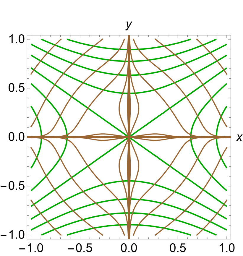
(a) For $\beta_{\bf e}=-1/2$.

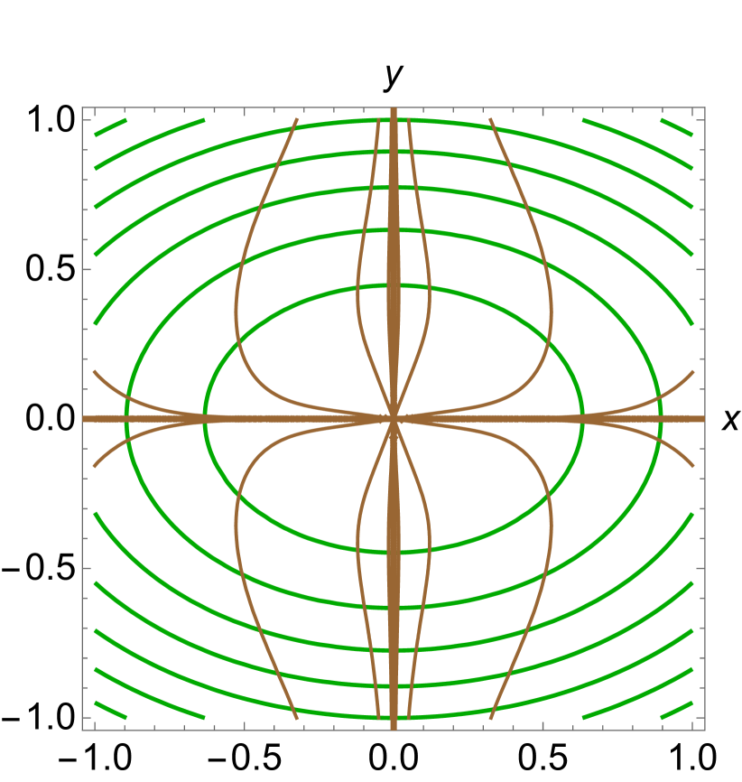
(b) For $\beta_{\bf e}=1/2$.

Figure 10: Gradient flow orbits of $V$ (shown in brown) and level sets of $V$ (shown in green) near a critical horn end ${\bf e}$, drawn in principal Cartesian canonical coordinates centered at ${\bf e}$ for two values of $\beta_{\bf e}$.

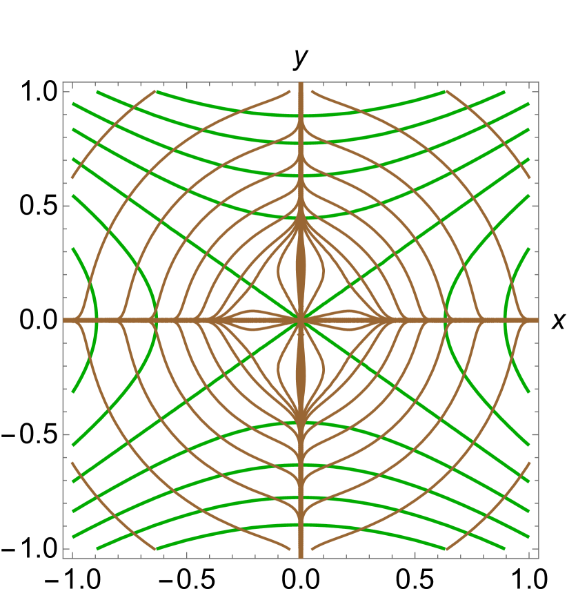
(a) For $\beta_{\bf e}=-1/2$.

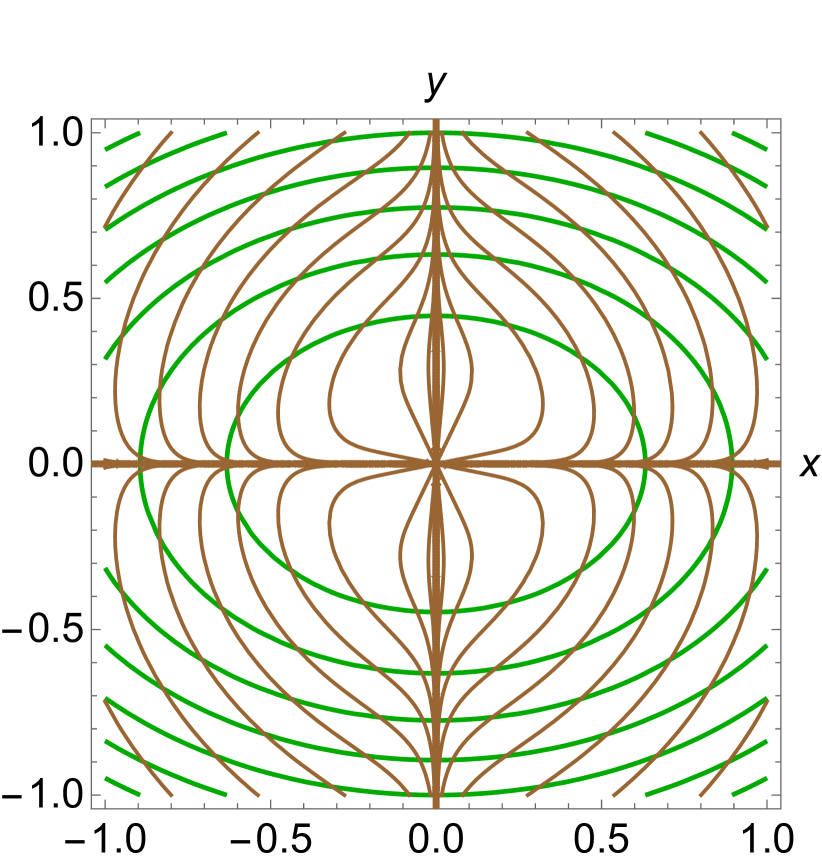
(b) For $\beta_{\bf e}=1/2$.

Figure 11: Gradient flow orbits of $V$ (shown in brown) and level sets of $V$ (shown in green) near a critical funnel end ${\bf e}$ of circumference $\ell=1$, drawn in principal Cartesian canonical coordinates centered at ${\bf e}$ for two values of $\beta_{\bf e}$.

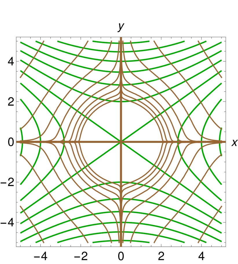
(a) For $\beta_{\bf e}=-1/2$.

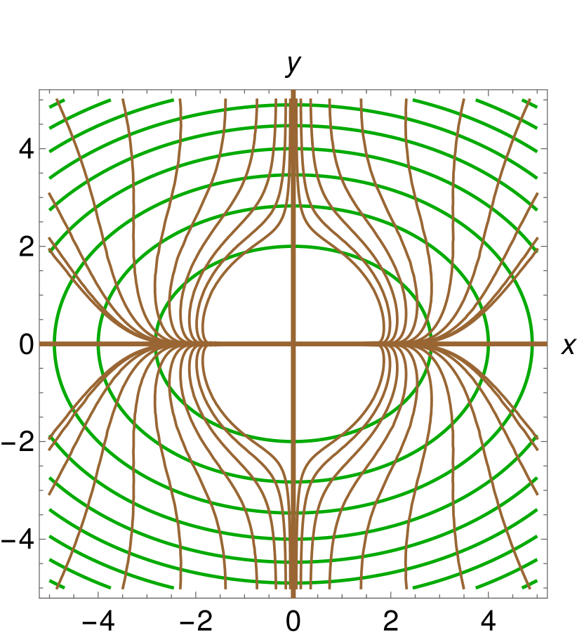
(b) For $\beta_{\bf e}=1/2$.

Figure 12: Gradient flow orbits of $V$ (shown in brown) and level sets of $V$ (shown in green) near a critical cusp end ${\bf e}$, drawn in principal Cartesian canonical coordinates centered at ${\bf e}$ for two values of $\beta_{\bf e}$.

The extended scalar potential ${\hat{\Phi}}$ of the canonical model can be recovered from the extended classical effective potential as:

$${\hat{\Phi}}=\frac{1}{2M_{0}^{2}}\widehat{V}^{2}\approx\frac{{\bar{\lambda}}_{2}({\bf e})^{2}}{2}\left[\hat{\bar{V}}({\bf e})+\frac{1}{2}\omega^{2}(\beta_{\bf e}\cos^{2}\theta+\sin^{2}\theta)\right]^{2}~{}~{},$$ (63)

where we defined:

$${\bar{\lambda}}_{2}({\bf e})\stackrel{{\scriptstyle{\rm def.}}}{{=}}\frac{\lambda_{2}({\bf e})}{M_{0}}~{}~{},~{}~{}{\hat{\bar{V}}}({\bf e})\stackrel{{\scriptstyle{\rm def.}}}{{=}}\frac{{\hat{V}}({\bf e})}{\lambda_{2}({\bf e})}~{}~{}.$$

Figures 13-16 show some numerically computed infrared optimal cosmological orbits of the canonical model parameterized by $(M_{0},\Sigma,G,\Phi)$ near critical ends ${\bf e}$. In these figures, we took ${\bar{\lambda}}_{2}({\bf e})=1$, ${\bar{\hat{V}}}({\bf e})=1$ and $M_{0}=1$. Notice that the accuracy of the first order IR approximation depends on the value of ${\hat{\bar{V}}}({\bf e})$, since the first IR parameter of ren depends on this value. The initial point of each orbit is shown as a black dot.

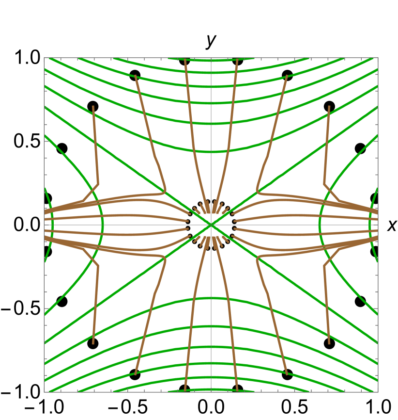
(a) For $\beta_{\bf e}=-1/2$

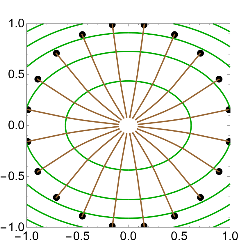
(b) For $\beta_{\bf e}=1/2$

Figure 13: Numerically computed infrared optimal cosmological orbits of the canonical model (shown in brown) and level sets of ${\hat{\Phi}}$ (shown in green) near a critical plane end ${\bf e}$, drawn in principal canonical Cartesian coordinates centered at ${\bf e}$ for two values of $\beta_{\bf e}$.

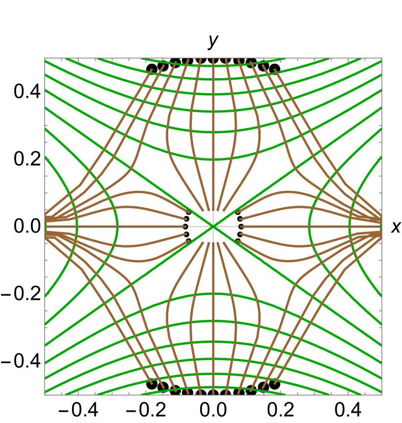
(a) For $\beta_{\bf e}=-1/2$.

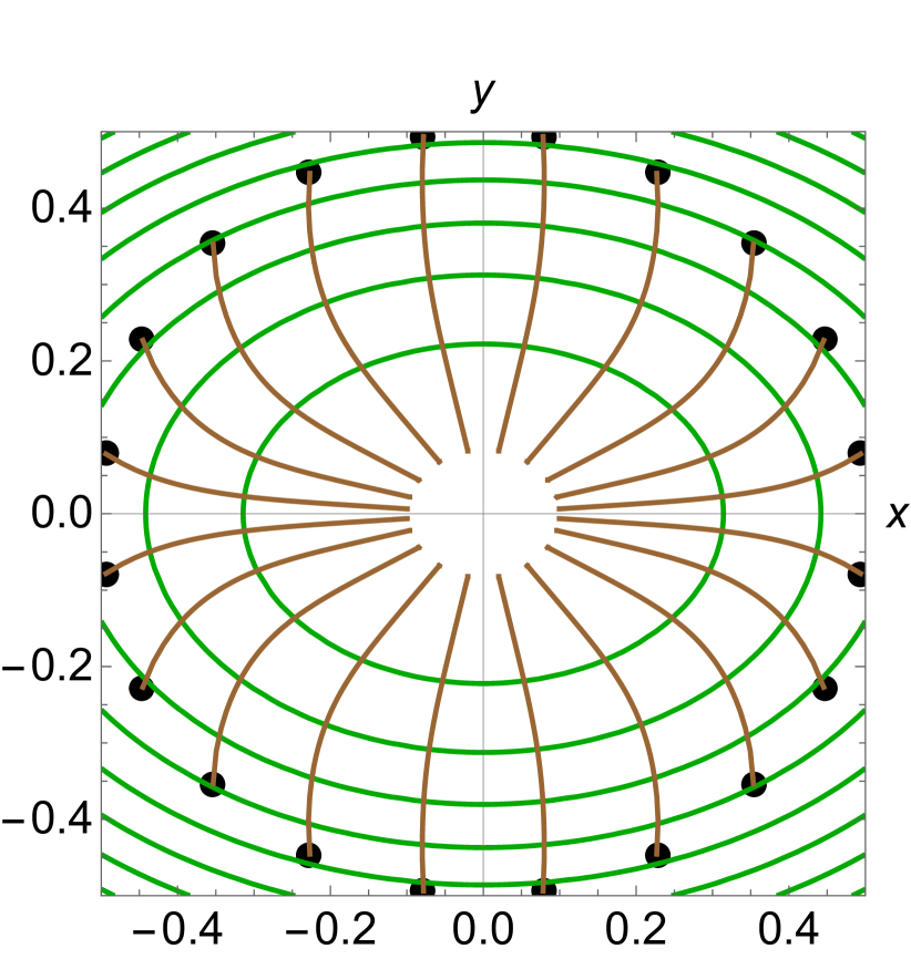
(b) For $\beta_{\bf e}=1/2$.

Figure 14: Numerically computed infrared optimal cosmological orbits of the canonical model (shown in brown) and level sets of ${\hat{\Phi}}$ (shown in green) near a critical horn end ${\bf e}$, drawn in principal canonical Cartesian coordinates centered at ${\bf e}$ for two values of $\beta_{\bf e}$.

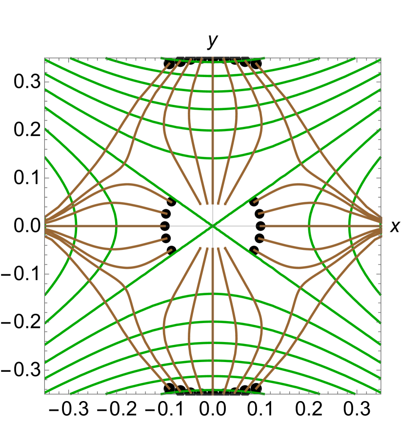
(a) For $\beta_{\bf e}=-0.5$.

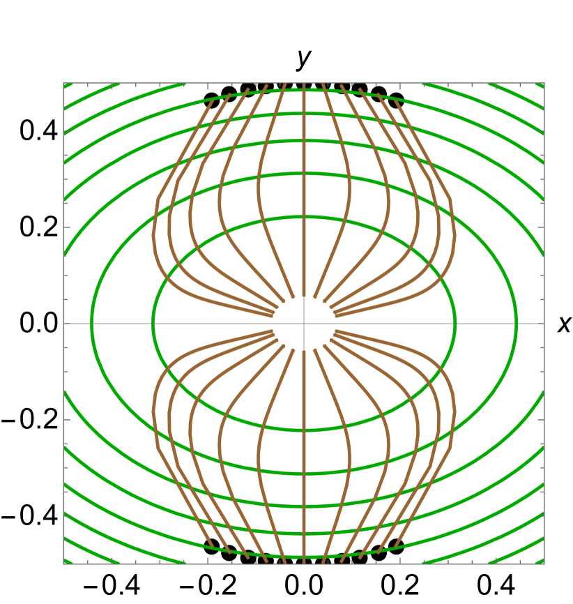
(b) For $\beta_{\bf e}=0.5$.

Figure 15: Numerically computed infrared optimal cosmological orbits of the canonical model (shown in brown) and level sets of ${\hat{\Phi}}$ (shown in green) near a critical funnel end ${\bf e}$ of circumference $\ell=1$, drawn in principal canonical coordinates centered at ${\bf e}$ for two values of $\beta_{\bf e}$.

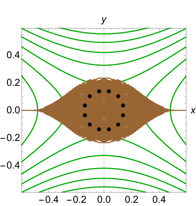
(a) For $\beta_{\bf e}=-0.5$.

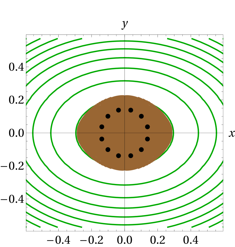
(b) For $\beta_{\bf e}=0.5$.

Figure 16: Numerically computed infrared optimal cosmological orbits of the canonical model (shown in brown) and level sets of ${\hat{\Phi}}$ (shown in green) near a critical cusp end ${\bf e}$, drawn in principal canonical coordinates centered at ${\bf e}$ for two values of $\beta_{\bf e}$.

The case of critical cusp ends is particularly interesting. For clarity, Figures 17 and 18 display the evolution of a single infrared optimal cosmological curve of the uniformized model for four consecutive cosmological times when $\beta_{\bf e}<0$ and $\beta_{\bf e}>0$ respectively, where in the second case we assume that ${\bf e}$ is a local minimum of $\widehat{V}$; this orbit was chosen such that its initial point does not lie on any of the four principal geodesic orbits. When $\beta_{\bf e}<0$, the orbit spirals numerous times around the cusp while approaching it, after which it spirals away from the cusp until it is finally repelled by it along one of two principal geodesic orbits. When $\beta_{\bf e}>0$ (and assuming as in Figure 18 that ${\bf e}$ is a local minimum of $\widehat{V}$), the cosmological orbit first spirals around the cusp end approaching it, after which it distances from it oscillating with gradually decreasing amplitude around one of the principal geodesic orbits until stopped by the attractive force generated by the scalar potential. At that point the cosmological curve starts evolving back towards the cusp and “falls back into” the cusp end along the principal geodesic. On the other hand, infrared optimal cosmological curves which start from a point lying on one of the four principal geodesic orbits flow away from the cusp or into it along that geodesic depending on whether the cusp is a source, sink or saddle for $\widehat{V}$ (and, in the saddle case, on the choice of that principal geodesic).

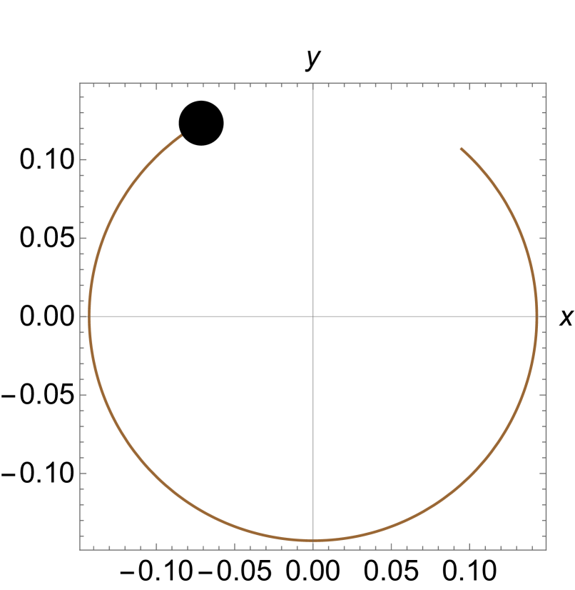
(a) For $t=0.000008$.

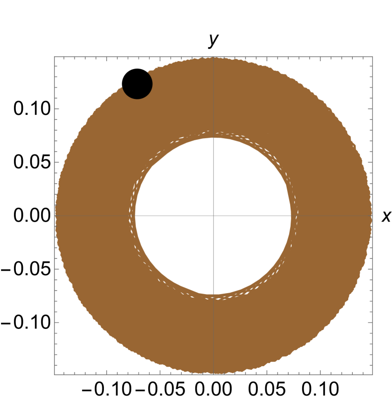
(b) For $t=0.01$.

(c) For $t=0.5$.

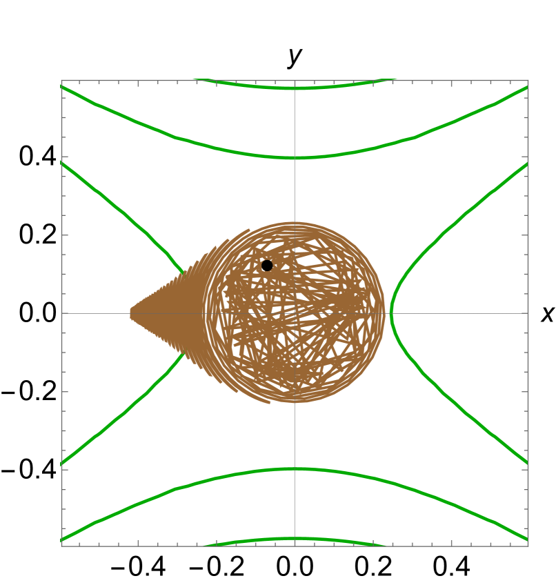
(d) For $t=5$.

Figure 17: A numerically computed infrared optimal cosmological orbit of the canonical model (shown in brown) and level sets of ${\hat{\Phi}}$ (shown in green) near a critical cusp end ${\bf e}$ for $\beta_{\bf e}=-1/2$. The trajectory starts at $\omega(0)=\frac{1}{7}$ and $\theta(0)=\frac{2\pi}{3}$ with initial speed in the gradient flow shell of $(\Sigma,G,V)$. The four figures show the cosmological orbit for cosmological times between $t=0$ and $t=0.000008$, $0.01$, $0.5$ and $5$ respectively. The white interior areas in the last figure are numerical artifacts due to limited float precision.

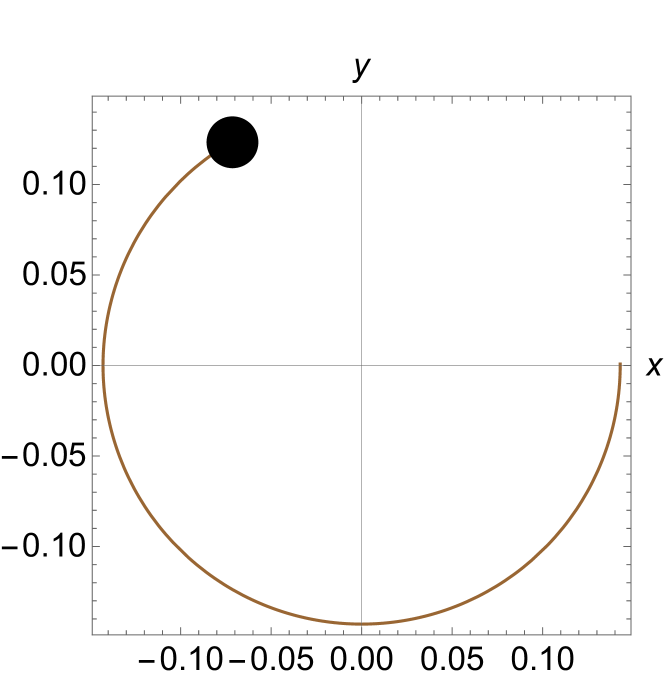
(a) For $t=0.00002$.

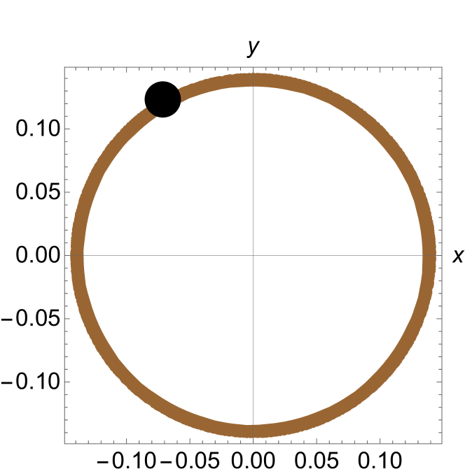
(b) For $t=0.01$.

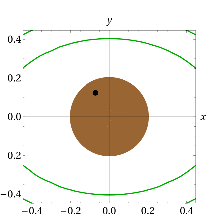
(c) For $t=0.5$.

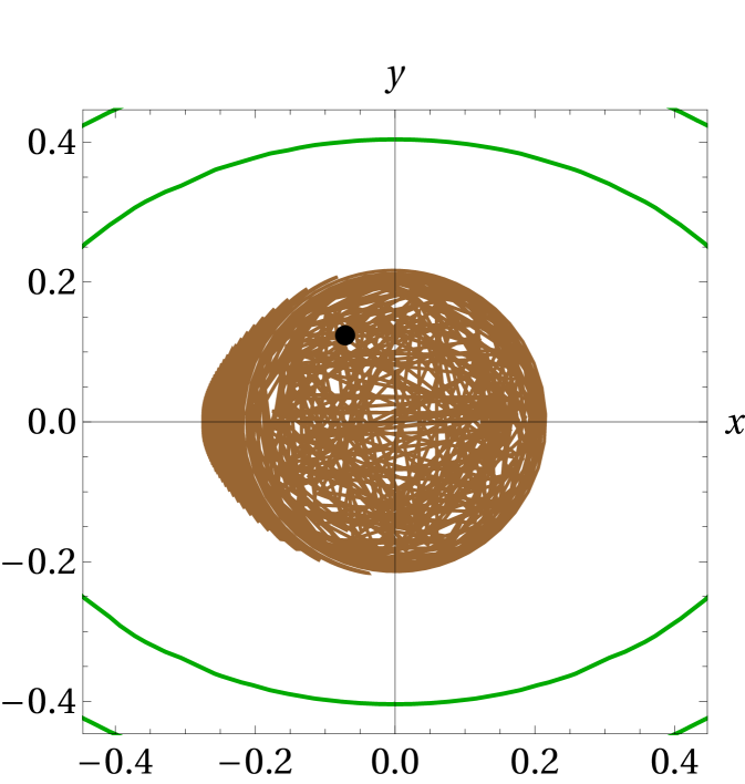
(d) For $t=5$.

Figure 18: A numerically computed infrared optimal cosmological orbit of the canonical model (shown in brown) and level sets of ${\hat{\Phi}}$ (shown in green) near a critical cusp end ${\bf e}$ for $\beta_{\bf e}=+1/2$ when the cusp end is a local minimum of $\widehat{V}$. The trajectory starts at $\omega(0)=\frac{1}{7}$ and $\theta(0)=\frac{2\pi}{3}$ with initial speed in the gradient flow shell of $(\Sigma,G,V)$. The four figures show the orbit for cosmological times between $t=0$ and $t=0.00002$, $0.01$, $0.5$ and $5$ respectively. The white interior areas in the last figure are numerical artifacts due to limited float precision.

5.3 Stable and unstable manifolds of critical ends under the effective gradient flow

The analysis above shows that critical ends of $\Sigma$ behave like exotic fixed points of the gradient flow of $(\Sigma,G,V)$. The dimensions and number of connected components of the stable and unstable manifolds (in $\Sigma$) are listed below, where we use the notations:

$$\mathcal{A}_{+}({\bf e})\stackrel{{\scriptstyle{\rm def.}}}{{=}}\mathcal{S}({\bf e})~{}~{} ~{}~{}\mathcal{A}_{-}({\bf e})\stackrel{{\scriptstyle{\rm def.}}}{{=}}\mathcal{U}({\bf e})~{}~{}$$ ,

$$d_{+}({\bf e})\stackrel{{\scriptstyle{\rm def.}}}{{=}}\dim\mathcal{S}({\bf e})~{}~{} ~{}~{}d_{-}({\bf e})\stackrel{{\scriptstyle{\rm def.}}}{{=}}\dim\mathcal{U}({\bf e})~{}~{}$$ ,

$$n_{+}({\bf e})\stackrel{{\scriptstyle{\rm def.}}}{{=}}\mathrm{Card}[\pi_{0}(\mathcal{S}({\bf e}))]~{}~{} ~{}~{}n_{-}({\bf e})\stackrel{{\scriptstyle{\rm def.}}}{{=}}\mathrm{Card}[\pi_{0}(\mathcal{U}({\bf e}))]~{}~{}.$$ ,

1. If ${\bf e}$ is a flaring end:

   • $\beta_{\bf e}\in[-1,0)$ (i.e. ${\bf e}$ is a saddle point of $\widehat{V}$): $d_{+}({\bf e})=d_{-}({\bf e})=2$, $n_{+}({\bf e})=n_{-}({\bf e})=2$

   • $\beta_{\bf e}\in(0,1]$ (i.e. ${\bf e}$ is an extremum of $\widehat{V}$): Then $\epsilon_{1}({\bf e})=\epsilon_{2}({\bf e}):=\epsilon\in\{-1,1\}$ and $d_{\epsilon}({\bf e})=2$, $n_{\epsilon}({\bf e})=1$ with $\mathcal{A}_{-\epsilon}=\emptyset$.

2. If ${\bf e}$ is a cusp end:

   • $\beta_{\bf e}\in[-1,0)$ (i.e. ${\bf e}$ is a saddle point of $\widehat{V}$): $d_{+}({\bf e})=d_{-}({\bf e})=1$, $n_{+}({\bf e})=n_{-}({\bf e})=2$

   • $\beta_{\bf e}\in(0,1]$ (i.e. ${\bf e}$ is an extremum of $\widehat{V}$): Then $\epsilon_{1}({\bf e})=\epsilon_{2}({\bf e})=\epsilon\in\{-1,1\}$ and $d_{\epsilon}({\bf e})=2$, $n_{\epsilon}({\bf e})=1$ with $\mathcal{A}_{-\epsilon}=\emptyset$.

Notice that the stable and unstable manifolds of an end are subsets of $\Sigma$ and that the number of their connected components depends on the fact that the Freudenthal ends are not points of $\Sigma$.

6 Conclusions and further directions

We studied the first order IR approximants of hyperbolizable tame two-field models, which are defined by the conditions that the target surface $\Sigma$ is oriented and has finitely-generated fundamental group, that the scalar field metric $\mathcal{G}$ is hyperbolizable and that the scalar potential $\Phi$ admits a strictly positive and smooth Morse extension ${\hat{\Phi}}$ to the end compactification of $\Sigma$. In this situation, the asymptotic form of the gradient flow orbits of the uniformized effective scalar triple $(\Sigma,G,V)$ (which describe the asymptotic behavior of the first IR approximant of the two-field model parameterized by $(\Sigma,\mathcal{G},\Phi)$) can be determined explicitly near each critical point of the classical effective potential $V$ as well as near each end of $\Sigma$. We found that the gradient flow of $(\Sigma,G,V)$ has exotic behavior near the ends, which act like fictitious stationary points of this flow. Using results from the theory of geometrically finite hyperbolic surfaces, we showed that the IR behavior of the model near a critical point $c$ of the extended effective potential $\widehat{V}$ (which can be an interior critical point or a critical end) is characterized by the critical modulus $\beta_{c}\in[-1,1]\setminus\{0\}$ and by two sign factors $\epsilon_{1}(c),\epsilon_{2}(c)\in\{-1,1\}$ which satisfy the relation $\epsilon_{1}(c)\epsilon_{2}(c)=1$. When $c$ is a critical end, this behavior also depends on the hyperbolic type of that end. For critical ends, the definition of these quantities relies on the fact that the hyperbolic metric $G$ admits an $\mathrm{O}(2)$ symmetry in a vicinity of each end. For noncritical ends, we found that the asymptotic behavior of effective gradient flow orbits depends only on the hyperbolic type of the end. Non-critical flaring ends act like fictitious but exotic stationary points of the effective gradient flow even though they are not critical points of the extended effective potential.

These results characterize the infrared behavior in each IR phase of all tame two-field cosmological models up to first order in the infrared expansion of ren and hence open the way for systematic studies of such models. We note that tame two-field models form an extremely large class of cosmological models which was inaccessible until now to systematic or conceptual analysis. With the exception of the very special class of models discussed in Noether1 ; Noether2 (which admit a ‘hidden’ Noether symmetry and subsume all previously considered integrable two-field models with canonical kinetic term and canonical coupling to gravity), such models were approached before only with numerical methods. Moreover, the vast majority of work in this direction (with the exception of genalpha ; elem ; modular ) was concerned exclusively with the topologically trivial case of models whose target manifold is the Poincaré disk KLR . In view of ren and of the results of the present paper, models based on the Poincaré disk are extremely far from capturing the infrared universality classes of tame two-field models.

The results of this paper suggest various directions for further research. As an immediate extension, one can study in more generality the UV and IR behavior of two-field models whose target surface $\Sigma$ is a disk, a punctured disk or an annulus. In this case the uniformized scalar manifold $(\Sigma,G)$ is either an elementary Euclidean surface or an elementary hyperbolic surface. In the second situation, the universality classes are described by the UV or IR behavior of the elementary two-field $\alpha$-attractor models considered in elem . The geodesic flow on elementary hyperbolic surfaces (which describes the UV limit) is well-understood, while the effective gradient flow can be studied for potentials $V$ which admit a smooth extension $\widehat{V}$ to the Freudenthal compactification $\widehat{\Sigma}\simeq\mathrm{S}^{2}$ assuming that $\widehat{V}$ satisfies Morse-Bott conditions Bott on $\widehat{\Sigma}$. Similar questions can be asked for $n$-field models whose target manifold is an elementary hyperbolic space form Ratcliffe .

One could also study the IR approximation of models for which $(\Sigma,G)$ corresponds to a modular curve (such as the curve $Y(2)$ considered in modular ) with Morse-Bott conditions on the extended potential. Using the uniformization theorem, such problems can be reduced to the Poincaré disk, i.e. to studying the IR limit of a modular cosmological model in the sense of Sch1 ; Sch2 ; Sch3 ; Sch4 , though – as pointed out in genalpha ; modular – the quotient by the uniformization group can be highly nontrivial.

Finally, we mention that a characterization of the cosmological and effective gradient flow near the ends of $\Sigma$ up to topological equivalence can be extracted using the conformal compactification of $(\Sigma,G)$ and the Vishik normal form Vishik of vector fields near the conformal boundary of $\Sigma$ and near its lift to $T\Sigma$; we hope to report on this in a future publication.

Appendix A Details of computations for each case

This appendix gives some details of the computation of cosmological curves near critical points $c\in\widehat{\Sigma}$ of the extended potential. We take $M_{0}=1$ as explained in the main text. In principal Cartesian canonical coordinates near $c$, the first order approximation of the effective potential is:

$$V=V(c)+\frac{1}{2}\big{(}\lambda_{1}(c)x^{2}+\lambda_{2}(c)y^{2}\big{)}~{}~{},$$

with $V(c)$ a positive constant. We take $V(c)=1$ and $\lambda_{2}(c)=1$, which gives $\beta(c)\stackrel{{\scriptstyle{\rm def.}}}{{=}}\frac{\lambda_{1}(c)}{\lambda_{2}(c)}=\lambda_{1}(c)$. In polar principal canonical coordinates and with the assumptions considered, we have:

$$V=1+\frac{\omega^{2}}{2}\big{(}\beta(c)\cos^{2}\theta+\sin^{2}\theta\big{)}$$

In local coordinates on $\widehat{\Sigma}$, we have:

$$\nabla_{t}\dot{\varphi}^{i}(t)\!=\!\ddot{\varphi}^{i}(t)+\Gamma^{i}_{jk}(\varphi(t))\dot{\varphi}^{j}(t)\dot{\varphi}^{k}(t)~{},~{}~{}||\dot{\varphi}(t)||^{2}_{G}\!=\!G_{ij}(\varphi(t))\dot{\varphi}^{i}(t)\dot{\varphi}^{j}(t)~{},~{}~{}\mathrm{grad}_{G}\Phi\!=\!G^{ij}\partial_{i}\Phi\partial_{j}~{}.$$

An infrared optimal cosmological curve is a solution $\varphi(t)$ of the cosmological equation (4) which satisfies:

$${\dot{\varphi}}(0)=-(\mathrm{grad}_{G}V)(\varphi(0))~{}.$$

A.1 Interior critical points

In this case, $c$ is denoted by ${\bf c}$ and the hyperbolic metric $G$ has the following form in semigeodesic coordinates $(r,\theta)$ on the disk $D_{\omega_{\mathrm{max}}({\bf c})}$ (which is contained in the Poincaré disk $\mathbb{D}$):

$$\mathrm{d}s_{G}^{2}=\mathrm{d}r^{2}+\sinh^{2}(r)\mathrm{d}\theta^{2}~{}~{},$$

where $r$ is related to $\omega\stackrel{{\scriptstyle{\rm def.}}}{{=}}\sqrt{x^{2}+y^{2}}$ by $\omega=\tanh(r/2)$ and we have $r\leq r({\bf c})$. Notice that $(r,\theta)$ can be identified with the polar coordinates on the tangent space $T_{0}\mathbb{D}$ through the exponential map $\exp_{0}^{\mathbb{D}}$ of the Poincaré disk used in Subsection 3.1. The only nontrivial Christoffel symbols are:

$$\Gamma^{r}_{\theta\theta}=-\sinh(r)\cosh(r)~{}~{},~{}~{}\Gamma^{\theta}_{r\theta}=\Gamma^{\theta}_{\theta r}=\coth(r)~{}~{}.$$

The cosmological equations (4) become:

$$\ddot{r}-\frac{1}{2}\sinh(2r)\dot{\theta}^{2}+\dot{r}\sqrt{\dot{r}^{2}+\sinh^{2}(r)\dot{\theta}^{2}+2\Phi}+\partial_{r}\Phi=0~{}~{}$$

$$\ddot{\theta}+2\coth(r)\dot{r}\dot{\theta}+\dot{\theta}\sqrt{\dot{r}^{2}+\sinh^{2}(r)\dot{\theta}^{2}+2\Phi}+\frac{1}{\sinh^{2}(r)}\partial_{\theta}\Phi=0~{}~{},$$

which we solved numerically to obtain Figure 2. The scalar potential is $\Phi(r,\theta)=\frac{1}{2}V^{2}(r,\theta)$, where the classical effective potential takes the approximate form:

$$V(r,\theta)=1+\frac{1}{2}\tanh^{2}(r/2)\big{(}\beta({\bf c})\cos^{2}(\theta)+\sin^{2}(\theta)\big{)}~{}.$$

In principal polar canonical coordinates $(\omega,\theta)$ centered at ${\bf c}$, we have:

$$\mathrm{d}s^{2}_{G}=\frac{4}{(1-\omega^{2})^{2}}[\mathrm{d}\omega^{2}+\omega^{2}\mathrm{d}\theta^{2}]~{}~{}$$

and:

$$V(\omega,\theta)=1+\frac{1}{2}\omega^{2}\left[\lambda_{1}({\bf c})\cos^{2}\theta+\lambda_{2}({\bf c})\sin^{2}\theta\right]~{}~{}.$$

Thus:

$$H(\omega,\theta,\dot{\omega},\dot{\theta})=\sqrt{\frac{4}{(1-\omega^{2})^{2}}\big{(}\dot{\omega}^{2}+\omega^{2}\dot{\theta}^{2}\big{)}+2\Phi(\omega,\theta)}~{}~{}$$

$$\Gamma^{\omega}_{\omega\omega}=\frac{2\omega}{1-\omega^{2}}~{}~{},~{}~{}\Gamma^{\omega}_{\theta\theta}=-\omega^{2}\big{(}\frac{1}{\omega}+\frac{2\omega}{1-\omega^{2}}\big{)}~{}~{},~{}~{}\Gamma^{\theta}_{\omega\theta}=\Gamma^{\theta}_{\theta\omega}=\frac{1}{\omega}+\frac{2\omega}{1-\omega^{2}}~{}~{}$$

$$(\mathrm{grad}\Phi)^{\omega}\!\approx\!\frac{(1-\omega^{2})^{2}}{4}\partial_{\omega}\Phi~{}~{},~{}~{}(\mathrm{grad}\Phi)^{\theta}\!\approx\!\frac{(1-\omega^{2})^{2}}{4\omega^{2}}\partial_{\theta}\Phi$$

The cosmological equations become:

$$\ddot{\omega}+\Gamma^{\omega}_{\omega\omega}\dot{\omega}^{2}+\Gamma^{\omega}_{\theta\theta}\dot{\theta}^{2}+H\dot{\omega}+(\mathrm{grad}\Phi)^{\omega}=0~{},$$

$$\ddot{\theta}+2\Gamma^{\theta}_{\omega\theta}\dot{\omega}\dot{\theta}+H\dot{\theta}+(\mathrm{grad}\Phi)^{\theta}=0~{}~{}.$$

A.2 Critical and noncritical ends

Recall the asymptotic form (25) near the end ${\bf e}$ in principal polar canonical coordinates centered at ${\bf e}$:

$$\mathrm{d}s_{G}^{2}|_{\dot{U}_{\bf e}}=\frac{\mathrm{d}\omega^{2}}{\omega^{4}}+f_{\bf e}(1/\omega)\mathrm{d}\theta^{2}~{}~{},$$

with:

$$f_{\bf e}(1/\omega)={\tilde{c}}_{\bf e}e^{\frac{2\epsilon_{\bf e}}{\omega}}\left[1+\mathrm{O}\left(e^{-\frac{2}{\omega}}\right)\right]~{}~{}\mathrm{for}~{}~{}\omega\ll 1~{}~{},$$

where:

$${\tilde{c}}_{\bf e}=\left\{\begin{array}[]{ll}\frac{1}{4}&\mbox{if}~{}{\bf e}=\mathrm{plane~{}end}\\ \frac{1}{(2\pi)^{2}}&\mbox{if}~{}{\bf e}=\mathrm{horn~{}end}\\ \frac{\ell^{2}}{(4\pi)^{2}}&\mbox{if}~{}{\bf e}=\mathrm{funnel~{}end~{}of~{}circumference}~{}\ell>0\\ \frac{1}{(2\pi)^{2}}&\mbox{if}~{}{\bf e}=\mathrm{cusp~{}end}\end{array}\right.$$

and:

$$\epsilon_{\bf e}=\left\{\begin{array}[]{ll}+1&\mbox{if }~{}{\bf e}=\mathrm{flaring~{}(i.e.~{}plane,~{}horn~{}or~{}funnel)~{}end}\\ -1&\mbox{if }~{}{\bf e}=\mathrm{cusp~{}end}\end{array}\right.~{}~{}.$$

The term $\mathrm{O}\left(e^{-\frac{2}{\omega}}\right)$ vanishes identically when ${\bf e}$ is a cusp or horn end, but we will approximate it to zero for all ends. The only nontrivial Christoffel symbols are:

$$\Gamma^{\omega}_{\omega\omega}=-\frac{2}{\omega}~{}~{},~{}~{}\Gamma^{\omega}_{\theta\theta}=\tilde{c}_{\bf e}\epsilon_{\bf e}\omega^{2}{\bf e}^{\frac{2\epsilon_{\bf e}}{\omega}}~{}~{},~{}~{}\Gamma^{\theta}_{\theta\omega}=\Gamma^{\theta}_{\omega\theta}=-\frac{\epsilon_{\bf e}}{\omega^{2}}~{}~{}.$$

The cosmological equations (4) become:

$$\ddot{\omega}-\frac{2}{\omega}\dot{\omega}^{2}+\tilde{c}_{\bf e}\epsilon_{\bf e}\omega^{2}e^{\frac{2\epsilon_{\bf e}}{\omega}}\dot{\theta}^{2}+H\dot{\omega}+\omega^{4}\partial_{\omega}\Phi=0~{}~{},$$

$$\ddot{\theta}-\frac{2\epsilon_{\bf e}}{\omega^{2}}\dot{\omega}\dot{\theta}+H\dot{\theta}+\frac{1}{\tilde{c}_{\bf e}}e^{-\frac{2\epsilon_{\bf e}}{\omega}}\partial_{\theta}\Phi=0~{}~{},$$ (64)

where

$$H=\sqrt{\frac{\dot{\omega}^{2}}{\omega^{4}}+\tilde{c}_{\bf e}e^{\frac{2\epsilon_{\bf e}}{\omega}}\dot{\theta}^{2}+2\Phi}~{}~{}.$$

The difference between the critical and noncritical ends manifests in the form of the second order approximations for the potential:

$\bullet$ for critical ends:

$$V(\omega,\theta)=1+\frac{1}{2}\omega^{2}\big{(}\beta({\bf e})\cos^{2}\theta+\sin^{2}\theta\big{)}~{},$$

$\bullet$ for the noncritical ends:

$$V(\omega,\theta)=1+\mu\omega\cos\theta~{},$$

where $\mu_{\bf e}$ is a positive constant which we chose to be $1/2$ in our graphs.

Figures 5, 6, and 13-18 were obtained by solving (A.2) numerically in each case.

References

- (1) C. Vafa, The string landscape and the swampland, arXiv:hep-th/0509212.
- (2) H. Ooguri, C. Vafa, On the geometry of the string landscape and the swampland, Nucl. Phys. B 766 (2007) 21-33, arXiv:hep-th/0605264.
- (3) T. D. Brennan, F. Carta, C. Vafa, The String Landscape, the Swampland, and the Missing Corner, TASI2017 (2017) 015, arXiv:1711.00864 [hep-th].
- (4) M. van Beest, J. Calderon-Infante, D. Mirfendereski, I. Valenzuela, Lectures on the Swampland Program in String Compactifications, arXiv:2102.01111 [hep-th].
- (5) A. Achucarro, G. A. Palma, The string swampland constraints require multi-field inflation, JCAP 02 (2019) 041, arXiv:1807.04390 [hep-th].
- (6) G. Obied, H. Ooguri, L. Spodyneiko, C. Vafa, De Sitter Space and the Swampland, arxiv:1806.08362 [hep-th].
- (7) S.K. Garg, C. Krishnan, Bounds on Slow Roll and the de Sitter Swampland, JHEP 11 (2019) 075, arXiv:1807.05193 [hep-th].
- (8) R. D’Agostino, O. Luongo, Cosmological viability of a double field unified model from warm inflation, arXiv:2112.12816 [astro-ph.CO].
- (9) C. I. Lazaroiu, Dynamical renormalization and universality in classical multifield cosmological models, arXiv:2202.13466 [hep-th].
- (10) C. I. Lazaroiu, C. S. Shahbazi, Generalized two-field -attractor models from geometrically finite hyperbolic surfaces, Nucl. Phys. B 936 (2018) 542-596.
- (11) E. M. Babalic, C. I. Lazaroiu, Generalized -attractor models from elementary hyperbolic surfaces, Adv. Math. Phys. 2018 (2018) 7323090, arXiv:1703.01650.
- (12) E. M. Babalic, C. I. Lazaroiu, Generalized -attractors from the hyperbolic triply-punctured sphere, Nucl. Phys. B 937 (2018) 434-477, arXiv:1703.06033.
- (13) L. Anguelova, E. M. Babalic, C. I. Lazaroiu, Two-field Cosmological -attractors with Noether Symmetry, JHEP 04 (2019) 148, arXiv:1809.10563 [hep-th].
- (14) L. Anguelova, E. M. Babalic, C. I. Lazaroiu, Hidden symmetries of two-field cosmological models, JHEP 09 (2019) 007, arXiv:1905.01611 [hep-th].
- (15) L. Anguelova, On Primordial Black Holes from Rapid Turns in Two-field Models, JCAP 06 (2021) 004, arXiv:2012.03705 [hep-th].
- (16) L. Anguelova, J. Dumancic, R. Gass, L. C. R. Wijewardhana, Dark Energy from Inspiraling in Field Space, arXiv:2111.12136 [hep-th].
- (17) C. I. Lazaroiu, Hesse manifolds and Hessian symmetries of multifield cosmological models, Rev. Roum. Math. Pures Appl. 66 (2021) 2, 329-345, arXiv:2009.05117 [hep-th].
- (18) E. M. Babalic, C. I. Lazaroiu, Two-field cosmological models and the uniformization theorem, Springer Proc. Math. Stat., Quantum Theory and Symmetries with Lie Theory and Its Applications in Physics 2 (2018) 233-241.
- (19) E. M. Babalic, C. I. Lazaroiu, Cosmological flows on hyperbolic surfaces, Facta Universitatis, Ser. Phys. Chem. Tech. 17 (2019) 1, 1-9.
- (20) L. Anguelova, E. M. Babalic, C. I. Lazaroiu, Noether Symmetries of Two-Field Cosmological Models, AIP Conf. Proc. 2218 (2020) 050005.
- (21) L. Anguelova, Primordial Black Hole Generation in a Two-field Inflationary Model, arXiv:2112.07614 [hep-th].
- (22) J. Palis Jr., W. De Melo, Geometric theory of dynamical systems: an introduction, Springer, New York, U.S.A. (2012).
- (23) A. Katok, B. Hasselblatt, Introduction to the modern theory of dynamical systems, Cambridge U.P., 1995.
- (24) H. Freudenthal, Über die Enden topologischer Räume und Gruppen, Math. Z. 33 (1931) 692-713.
- (25) H. Freudenthal, Neuaufbau der Endentheorie, Ann. of Math. 43 (1942) 2, 261-279.
- (26) H. Freudenthal, Über die Enden diskreter Räume und Gruppen, Comm. Math. Helv. 17 (1945), 1-38.
- (27) B. Kerekjarto, Vorlesungen über Topologie I, Springer, Berlin, 1923.
- (28) S. Stoilow, Lecons sur les principes topologiques de la théorie de fonctions analytiques, 2nd ed., Gauthier-Villars, Paris, 1956.
- (29) I. Richards, On the Classification of Non-Compact Surfaces, Trans. AMS 106 (1963) 2, 259-269.
- (30) J. Szilasi, R. L. Lovas, D. C. Kertesz, Connections, sprays and Finsler structures, World Scientific, 2014.
- (31) J. Milnor, Morse theory, Annals of Math. Studies 51, Princeton, 1963.
- (32) R. Bott, Lectures on Morse theory, old and new, Bull. Amer. Math. Soc. (N.S.) 7 (1982) 2, 331-358.
- (33) P. Kronheimer, T. Mrowka, Monopoles and three manifolds, Cambridge, 2007.
- (34) F. Laudenbach, A Morse complex on manifolds with boundary, Geom. Dedicata 153 (2011) 47-57.
- (35) M. Akaho, Morse homology and manifolds with boundary, Commun. Contemp. Math. 9 (2007) 3, 301-334; see also Morse homology of manifolds with boundary revisited, arXiv:1408.1474 [math.SG] .
- (36) P. Petersen, Riemannian geometry, Graduate Texts in Mathematics, 3rd ed., 2016.
- (37) D. Borthwick, Spectral Theory of Infinite-Area Hyperbolic Surfaces, Progress in Mathematics 256, Birkhäuser, Boston, 2007.
- (38) J. G. Ratcliffe, Foundations of Hyperbolic Manifolds, Graduate Texts in Mathematics 149, Springer, 2006.
- (39) R. Kallosh, A. Linde, D. Roest, Superconformal Inflationary -Attractors, JHEP 11 (2013) 098, arXiv:1311.0472 [hep-th].
- (40) R. Schimmrigk, Modular inflation observables and j-inflation phenomenology, JHEP 09 (2017) 043, arXiv:1612.09559 [hep-th].
- (41) R. Schimmrigk, Multifield Reheating after Modular j-Inflation, Phys. Lett. B 782 (2018) 193-197, arXiv:1712.09961 [hep-ph].
- (42) M. Lynker, R. Schimmrigk, Modular Inflation at Higher Level N, JCAP 06 (2019) 036, arXiv:1902.04625 [astro-ph.CO].
- (43) R. Schimmrigk, Large and small field inflation from hyperbolic sigma models, arXiv:2108.05400 [hep-th].
- (44) S. M. Vishik, Vector fields in the neighborhood of the boundary of a manifold, Vestnik Moskov. Univ. Ser. I Mat. Mech., 27 (1972) 1, 21-28.