A general class of linear unconditionally energy stable schemes for the gradient flows

Abstract

This paper studies a class of linear unconditionally energy stable schemes for the gradient flows. Such schemes are built on the SAV technique and the general linear time discretization (GLTD) as well as the linearization based on the extrapolation for the nonlinear term, and may be arbitrarily high-order accurate and very general, containing many existing SAV schemes and new SAV schemes. It is shown that the semi-discrete-in-time schemes are unconditionally energy stable when the GLTD is algebraically stable, and are convergent with the order of $\min\{\hat{q},\nu\}$ under the diagonal stability and some suitable regularity and accurate starting values, where $\hat{q}$ is the generalized stage order of the GLTD and $\nu$ denotes the number of the extrapolation points in time. The energy stability results can be easily extended to the fully discrete schemes, for example, if the Fourier spectral method is employed in space when the periodic boundary conditions are specified. Some numerical experiments on the Allen-Cahn, Cahn-Hilliard, and phase field crystal models are conducted to validate those theories as well as the effectiveness, the energy stability and the accuracy of our schemes.

1 Introduction

Many physical problems arisen in science and engineering can be modeled by partial differential equations in the form of gradient flows, for example, the interface dynamics [3, 31, 79], the crystal growth [8, 44, 63], the tumor growth [54, 69], the thin film [66, 43], the polymers [27, 26, 53], the solidification [7, 42, 65] and so on. The gradient flows are dynamics determined by not only the driving free energy, but also the dissipation mechanism. For a given free energy $\mathcal{F}(u)$, the gradient flows can be written as

$$\frac{\partial u}{\partial t}=\mathcal{G}\mu,$$ (1.1)

supplemented with suitable boundary conditions (e.g. with periodic or homogeneous Neumann boundary conditions) [60], where $\mu=\delta\mathcal{F}/\delta u$ denotes the variational derivative of $\mathcal{F}(u)$ and the operator $\mathcal{G}$ is non-positive symmetric so that the free energy is monotonically decreasing

$$\frac{d\mathcal{F}(u)}{dt}=\left(\frac{\delta\mathcal{F}}{\delta u},\frac{\partial u}{\partial t}\right)=(\mu,\mathcal{G}\mu)\leq 0,$$ (1.2)

here $(\cdot,\cdot)$ denotes the inner product in $L^{2}(\Omega)$. If $\mathcal{G}=-I$ (resp. $\Delta$), then one has the so-called $L^{2}$ (resp. $H^{-1}$) gradient flow.

Most of gradient flow equations are nonlinear so that it is hard to obtain their analytical solutions. Hence, studying them numerically is the primary approach. Recently, designing efficient and energy stable numerical schemes for the gradient flows has attracted much attention. There exist several efficient and popular techniques to design energy stable schemes for the gradient flows. The first is the convex splitting [23, 24]. Based on it, one can design unconditionally energy stable and uniquely solvable schemes, but should solve a nonlinear system at each time step generally. Although the convex splitting technique has been developed case-by-case for some problems [5, 57, 71], it is not available to give an unified formulation. The second technique is the stabilization [62, 56, 64], which treats the nonlinear terms explicitly and adds a stabilization term to relax the time step constraint. It is simple and efficient since the linear equations with constant coefficients are solved at each time step. However, it is very challenging to design high-order unconditionally energy stable schemes. Some progresses can be found in [47]. The third technique is the invariant energy quadratization (IEQ) [73, 74, 75, 77]. It allows one to construct the linear and second-order unconditionally energy stable schemes for a large class of the gradient flows, but needs to solve the linear equations with variable coefficients, and requires that the free energy density is bounded from below so that its applications are limited for some physically interesting models, such as the molecular beam epitaxial (MBE) model without slope selection [46]. The fourth technique is the scalar auxiliary variable (SAV) [58, 59, 60]. With the help of introducing some SAVs, the gradient flow model is reformulated into an equivalent form, then some linear and unconditionally energy stable schemes can be developed by approximating the reformulated system instead of the original gradient flow model. It is convenient to construct second-order or higher-order unconditionally energy stable SAV schemes, which need to solve several linear systems with constant coefficients at each time step. In addition to the above, there are some other interesting techniques, including but not limited to the exponential time differencing (ETD) [67, 22], the Lagrange multiplier [4, 30], the energy factorization [45, 68], and the averaged vector field [33] etc.

Up to now, the SAV technique may result in more robust schemes with less restrictions on the energy functionals and has been successfully applied to many existing gradient flow models [1, 17, 18, 29, 34, 36, 80, 51, 52, 78, 72]. However, in those existing works, the time discretizations are the backward Euler, the Crank-Nicolson (CN), or the second-order backward differentiation formula (BDF2), except the high-order SAV-RK (Runge-Kutta) [1, 29]. The aim of this paper is to study a general class of arbitrarily high-order linear unconditionally energy stable schemes for the gradient flows. Such schemes, abbreviated as the SAV-GL schemes below for convenience, are based on the SAV technique and the general linear time discretization (GLTD) as well as the linearization based on the extrapolation for the nonlinear term. It is worth noting that our studied SAV-GL schemes contain most of the time integration schemes (e.g. SAV-BDF1, SAV-CN, SAV-BDF2, SAV-RK etc.) for the gradient flows in literature and many new schemes. The GLTDs, as multistage multivalue schemes proposed in [9], can be considered as a natural generalization of the Runge-Kutta (RK) and linear multistep time discretizations, and are flexible in developing numerical methods with better stability and accuracy, except slightly complexity. Two special examples provided later are the so-called one-leg [19, 20] and multistep Runge-Kutta (MRK) [10, 49] time integration schemes.

The rest of this paper is organized as follows. Section 2 briefly reviews the GLTDs for the ordinary differential equations (ODEs) and extends them as a general class of semi-discrete-in-time linear schemes for the gradient flow equations by using the SAV and the linearization based on extrapolation. Specifically, the gradient flow equation is first changed as an equivalent form by using the SAV, and then the reformulated equation is approximated by the GLTDs, in which the linear part is implicitly discretized while the nonlinear part is explicitly and linearly dealt with the extrapolation. The energy stability and the convergence of the SAV-GL schemes are addressed in Sections 3 and 4, respectively. A discrete energy dissipation law is obtained in the sense of the weighted inner product and the norm if the GLTDs are algebraically stable, and the convergence order in time of $\min\{\hat{q},\nu\}$ is derived under some suitable regularity and accurate starting values, if the GLTDs are diagonal stable, where $\hat{q}$ is the generalized stage order of the GLTDs and $\nu$ denotes the number of the extrapolation points in time. Section 5 introduces the Fourier spectral discretization for the gradient flows with the periodic boundary conditions in order to conduct our numerical validation. Section 6 numerically tests the fully discrete SAV-GL schemes against three widely concerned gradient flow equations (which are the Allen-Cahn, Cahn-Hilliard, and phase field crystal models) in order to validate the effectiveness, energy stability and accuracy of our schemes. Some concluding remarks are given in Section 7.

2 SAV-GL schemes for gradient flows

This section briefly reviews the GLTDs [9, 12, 40] for the ODEs and extends them to the gradient flows by using the SAV technique [58, 59, 60] as a general class of linear numerical schemes, which will be abbreviated as “SAV-GL” below for convenience.

2.1 A brief review to GLTDs

For the first-order ODE

$$\frac{du}{dt}=u^{\prime}(t)=f(u(t)),~{}~{}t\in(0,T],$$ (2.1)

subject to the initial data $u(0)=u_{0}$, the GLTD is a large family of multistage multivalue schemes for ODEs, which includes the linear multistep, predictor-corrector and Runge-Kutta schemes as special cases. Many peoples have tried their best to search for the useful GLTDs which do not exist within the standard special cases, but possess as many of the advantages and as few of the disadvantages as possible. The readers are referred to the review paper [12] and the monograph [40] as well as references therein.

Assume that the time interval $[0,T]$ is divided into $K$ equal parts with the time stepsize $\tau\!=\!\frac{T}{K}$, $K\!\in\!\mathbb{Z}^{+}$. The GLTDs can be defined by

$$\begin{cases}~{}~{}U_{n,i}=\tau\sum\limits_{j=1}^{s}d_{ij}^{11}f(U_{n,i})+\sum\limits_{j=1}^{r}d_{ij}^{12}u_{j}^{[n]},~{}~{}~{}i=1,2,\cdots,s,\\[3.0pt] u_{i}^{[n+1]}=\tau\sum\limits_{j=1}^{s}d_{ij}^{21}f(U_{n,i})+\sum\limits_{j=1}^{r}d_{ij}^{22}u_{j}^{[n]},~{}~{}~{}i=1,2,\cdots,r,\end{cases}$$ (2.2)

where $d_{ij}^{\imath\jmath}\in\mathbb{R}$, $\imath,\jmath=1,2$, $U_{n,i}$ is an approximation of stage order $q$ to $u(t_{n}+c_{i}\tau)$, $c_{i}\in\mathbb{R}$, $i=1,\cdots,s$, and each of $r$ import quantities $\{u_{i}^{[n]}\}$ is an approximation of order $p\geq q$ to the linear combination of the scaled derivatives of the solution $u$ to (2.1) at $t_{n}$, i.e.

$$u_{i}^{[n]}=\sum\limits_{j=0}^{p}w_{ij}\tau^{j}u^{(j)}(t_{n})+{\mathcal{O}}(h^{p+1}),\ i=1,\cdots,r,\$$

with some scalars $w_{ij}$ and $u^{(j)}=\frac{d^{j}u}{dt^{j}}$. Such time discretizations are characterized by four integers $p,q,r,s$ (being respectively the method order, the stage order, the number of external approximations, and the number of stages or internal approximations), the abscissa vector $\mbox{\boldmath\small$c$}=(c_{1},c_{2},\cdots,c_{s})^{T}\in\mathbb{R}^{s}$, the vectors $\mbox{\boldmath\small$w$}_{j}=(w_{1j},w_{2j},\ldots,w_{rj})^{T}\in\mathbb{R}^{r}$, $j=0,1,\ldots,p$, and four coefficient matrices $\mbox{\boldmath\small$D$}_{\imath\jmath}=(d_{ij}^{\imath\jmath})$ for $\imath,\jmath=1,2$, where $\mbox{\boldmath\small$D$}_{11}\in\mathbb{R}^{s\times s},\mbox{\boldmath\small$D$}_{12}\in\mathbb{R}^{s\times r},\mbox{\boldmath\small$D$}_{21}\in\mathbb{R}^{r\times s}$ and $\mbox{\boldmath\small$D$}_{22}\in\mathbb{R}^{r\times r}$. Obviously, the GLTDs (2.2) are consistent with (2.1) if

$$\mbox{\boldmath\small$D$}_{21}\mbox{\boldmath\small$e$}+\mbox{\boldmath\small$D$}_{22}\mbox{\boldmath\small$w$}_{1}=\mbox{\boldmath\small$w$}_{0}+\mbox{\boldmath\small$w$}_{1},\ \ \mbox{\boldmath\small$D$}_{12}\mbox{\boldmath\small$w$}_{0}=\mbox{\boldmath\small$e$},\ \mbox{\boldmath\small$D$}_{22}\mbox{\boldmath\small$w$}_{0}=\mbox{\boldmath\small$w$}_{0},$$

where $\mbox{\boldmath\small$e$}=(1,1,\cdots,1)^{T}\in\mathbb{R}^{s}$. Moreover, for the stage consistency, one needs

$$\mbox{\boldmath\small$D$}_{11}\mbox{\boldmath\small$e$}+\mbox{\boldmath\small$D$}_{12}\mbox{\boldmath\small$w$}_{1}=\mbox{\boldmath\small$c$}.$$

For the self completeness, we introduce the definitions of the algebraical and diagonal stabilities and the generalized stage order, which will be used later.

Definition 2.1 ([40, Def. 2.9.8]).

A GLTD is algebraically stable (also called $G$-stable), if there exists a symmetric and positive definite matrix $\mbox{\boldmath\small$G$}\in\mathbb{R}^{r\times r}$ and a non-negative definite diagonal matrix $\mbox{\boldmath\small$H$}\in\mathbb{R}^{s\times s}$ such that the matrix

$$\mbox{\boldmath\small$M$}=\!\left[\!\begin{array}[]{*{4}{c}}\mbox{\boldmath\small$G$}-\mbox{\boldmath\small$D$}_{22}^{T}\mbox{\boldmath\small$G$}\mbox{\boldmath\small$D$}_{22}&\mbox{\boldmath\small$D$}_{12}^{T}\mbox{\boldmath\small$H$}-\mbox{\boldmath\small$D$}_{22}^{T}\mbox{\boldmath\small$G$}\mbox{\boldmath\small$D$}_{21}\vspace{0.1cm}\\ \mbox{\boldmath\small$H$}\mbox{\boldmath\small$D$}_{12}-\mbox{\boldmath\small$D$}_{21}^{T}\mbox{\boldmath\small$G$}\mbox{\boldmath\small$D$}_{22}&\mbox{\boldmath\small$D$}_{11}^{T}\mbox{\boldmath\small$H$}+\mbox{\boldmath\small$H$}\mbox{\boldmath\small$D$}_{11}-\mbox{\boldmath\small$D$}_{21}^{T}\mbox{\boldmath\small$G$}\mbox{\boldmath\small$D$}_{21}\end{array}\!\right]_{(r+s)\times(r+s)}\!,$$

is non-negative definite.

The algebraical stability is an important property, and the algebraically stable GLTDs can preserve the long time dynamics of dissipative ODEs [9]. Next section will show that the algebraically stable GLTDs with SAV may be unconditionally energy stable for the gradient flows (1.1).

Definition 2.2 ([49, Def. 1.2]).

A GLTD is diagonally stable if there exists a positive definite diagonal matrix $\tilde{\mbox{\boldmath\small$H$}}\in\mathbb{R}^{s\times s}$ such that the matrix $\tilde{\mbox{\boldmath\small$H$}}\mbox{\boldmath\small$D$}_{11}+\mbox{\boldmath\small$D$}_{11}^{T}\tilde{\mbox{\boldmath\small$H$}}\in\mathbb{R}^{s\times s}$ is positive definite.

The condition in this definition implies the coefficient matrix $\mbox{\boldmath\small$D$}_{11}$ is nonsingular [48] so that the diagonally stable GLTD is uniquely solvable. The diagonal stability will provide us convenience to derive the error estimates of the GLTDs.

Definition 2.3 ([49, Def. 1.5]).

The generalized stage order of the GLTD is $\hat{q}$, if $\hat{q}$ is the largest integer and there exist $\hat{u}_{i}(t_{n})$, $i=1,2,\cdots,r$, such that

$$\rho_{n,i}\!=\!\mathcal{O}(\tau^{\hat{q}+1}),~{}i\!=\!1,2,\cdots,s;~{}~{}\rho_{i}^{[n]}\!=\!\mathcal{O}(\tau^{\hat{q}+1}),~{}u_{i}(t_{n})\!-\!\hat{u}_{i}(t_{n})\!=\!\mathcal{O}(\tau^{\hat{q}}),~{}~{}i\!=\!1,2,\cdots,r,$$

where $u_{i}(t_{n}):=\sum\limits_{j=0}^{p}w_{ij}\tau^{j}u^{(j)}(t_{n})$, $\rho_{n,i}$ and $\rho_{i}^{[n]}$ are the local truncation errors given by

$$\begin{cases}u(t_{n,i})=\tau\sum\limits_{j=1}^{s}d_{ij}^{11}u^{\prime}(t_{n,j})+\sum\limits_{j=1}^{r}d_{ij}^{12}\hat{u}_{j}(t_{n})+\rho_{n,i},~{}~{}~{}i=1,2,\cdots,s,\\[3.0pt] \hat{u}_{i}(t_{n+1})=\tau\sum\limits_{j=1}^{s}d_{ij}^{21}u^{\prime}(t_{n,j})+\sum\limits_{j=1}^{r}d_{ij}^{22}\hat{u}_{j}(t_{n})+\rho_{i}^{[n]},~{}~{}~{}i=1,2,\cdots,r,\end{cases}$$ (2.3)

here $t_{n,j}=t_{n}+c_{j}\tau$, and $u(t)$ is the smooth solution of (2.1).

The generalized stage order of a GLTD is related to the stage order $q$ and the method order $p$ of the GLTD. Specifically, when a GLTD has the stage order $q$ and the method order $p=q$, taking $\hat{u}_{i}(t_{n})=u_{i}(t_{n})$ yields that the generalized stage order $\hat{q}$ is at least equal to $q$.

Remark 2.1.

The generalized stage order of some GLTDs is one higher than the stage order so that it can be used to obtain a sharper error estimate [49]. In fact, when a GLTD has the stage order $q$ and the method order $p=q+1$, it means that

$$\rho_{n,i}=\mathcal{O}(\tau^{q+1}),~{}~{}i=1,2,\cdots,s;~{}~{}~{}~{}\rho_{i}^{[n]}=\mathcal{O}(\tau^{q+2}),~{}~{}i=1,2,\cdots,r,$$

which are defined by (2.3) with $\hat{u}_{i}(t_{n})=u_{i}(t_{n})$. If there exists a constant $\kappa$ such that

$$\rho_{n,i}-\kappa\tau^{q+1}u^{(q+1)}(t_{n})=\mathcal{O}(\tau^{q+2}),~{}~{}~{}~{}i=1,2,\cdots,s,$$ (2.4)

and one chooses

$$\hat{u}_{i}(t_{n})=u_{i}(t_{n})+w_{i0}\kappa\tau^{q+1}u^{(q+1)}(t_{n}),$$

then using the consistency condition yields that the generalized stage order of the GLTD is $\hat{q}=q+1$.

Before ending this subsection, we introduce two typical examples of the GLTDs.

Example 2.1.

The first is the $r$-step one-leg time discretization [19, 20], which has the following form for (2.1)

$$\sum_{j=0}^{r}\alpha_{j}u^{n+1-j}=\tau f\left(\sum_{j=0}^{r}\beta_{j}u^{n+1-j}\right),$$ (2.5)

where $u^{n+1-j}\approx u(t_{n+1-j})$, $\alpha_{j},\beta_{j}\in\mathbb{R}$ satisfy $\alpha_{0}\beta_{0}\neq 0$ and the consistency conditions

$$\sum_{j=0}^{r}\alpha_{j}=0,~{}~{}\sum_{j=0}^{r}(1\!-\!j)\alpha_{j}=\sum_{j=0}^{r}\beta_{j}=1.$$

If setting $u_{i}^{[n]}=u^{n+1-i}$ for $i=1,2,\ldots,r$, which can be viewed as an approximation to $u_{i}(t_{n})$ with $\mbox{\boldmath\small$w$}_{0}=(1,1,\ldots,1)^{T}\in\mathbb{R}^{r}$ and $\mbox{\boldmath\small$w$}_{j}=\frac{1}{j!}\big{(}0,(-1)^{j},(-2)^{j},\ldots,(1\!-\!r)^{j}\big{)}^{T}\in\mathbb{R}^{r}$ for $j=1,2,\ldots,p$, and using

$$U_{n,1}=\sum_{j=0}^{r}\beta_{j}u^{n+1-j}=\sum_{j=1}^{r}\left(\beta_{j}\!-\!\frac{\beta_{0}}{\alpha_{0}}\alpha_{j}\right)u^{n+1-j}+\frac{\tau\beta_{0}}{\alpha_{0}}f\left(U_{n,1}\right),$$

to approximate $u(t_{n}+c_{1}\tau)$ with the consistency condition $c_{1}=\sum\limits_{j=0}^{r}(1\!-\!j)\beta_{j}$, then the scheme (2.5) has been reformulated as a GLTD form (2.2) with the coefficient matrices $\mbox{\boldmath\small$D$}_{\imath\jmath}$, $\imath,\jmath=1,2$, defined by

$$\mbox{\boldmath\small$D$}_{11}\!=\!\left[\frac{\beta_{0}}{\alpha_{0}}\right]_{1\times 1},~{}~{}~{}\mbox{\boldmath\small$D$}_{12}\!=\!\left[\beta_{1}\!-\!\frac{\beta_{0}}{\alpha_{0}}\alpha_{1},\beta_{2}\!-\!\frac{\beta_{0}}{\alpha_{0}}\alpha_{2},\cdots,\beta_{r}\!-\!\frac{\beta_{0}}{\alpha_{0}}\alpha_{r}\right]_{1\times r},$$

$$\mbox{\boldmath\small$D$}_{21}\!=\!\!\left[\!\begin{array}[]{*{5}{c}}1\\ 0\\ \vdots\\ 0\\ 0\end{array}\!\right]_{r\times 1},~{}~{}~{}~{}\mbox{\boldmath\small$D$}_{22}\!=\!\!\left[\!\begin{array}[]{*{25}{c}}-\frac{\alpha_{1}}{\alpha_{0}}&-\frac{\alpha_{2}}{\alpha_{0}}&\cdots&-\frac{\alpha_{r-1}}{\alpha_{0}}&-\frac{\alpha_{r}}{\alpha_{0}}\\ 1&0&\cdots&0&0\\ 0&1&\cdots&0&0\\ \vdots&\vdots&\ddots&\vdots&\vdots\\ 0&0&\cdots&1&0\end{array}\!\right]_{r\times r}.$$

The one-leg time discretization (2.5) is algebraically stable if and only if it is $A$-stable, see [20, Theorem 3.3]. Besides, if (2.5) is $A$-stable, then $\beta_{0}/\alpha_{0}\!>\!0$ so that (2.5) is diagonally stable. In our numerical experiments, we will use two special one-leg time discretizations. The first is

$$u^{n+1}=u^{n}+f\left(\theta u^{n+1}+(1-\theta)u^{n}\right),$$ (2.6)

where $\theta$ is a parameter. When $\frac{1}{2}\leq\theta\leq 1$, (2.6) is $A$-stable, and thus is algebraically stable and diagonally stable [19]. When (2.6) is written as a GLTD, the four parameters $\{p,q,r,s\}=\{1,1,1,1\}$ for $\frac{1}{2}<\theta\leq 1$ and $\{p,q,r,s\}=\{2,1,1,1\}$ for (2.6) with $\theta=\frac{1}{2}$. The second is a class of two-step schemes

$$\frac{1\!+\!\gamma}{2}u^{n+1}=\gamma u^{n}-\frac{\gamma\!-\!1}{2}u^{n-1}+f\left(\frac{1\!+\!\gamma\!+\!\delta}{4}u^{n+1}+\frac{1\!-\!\delta}{2}u^{n}+\frac{1\!-\!\gamma\!+\!\delta}{4}u^{n-1}\right),$$ (2.7)

where $\gamma$ and $\delta$ are two parameters. If $\gamma\geq 0$ and $\delta>0$, then (2.7) is $A$-stable [19], and thus is algebraically stable and diagonally stable. Four integers $\{p,q,r,s\}=\{2,1,2,1\}$ for (2.7) as a GLTD. ∎

Example 2.2.

Another important subclass of the GLTDs (2.2) are the multistep Runge-Kutta (MRK) time discretizations, see e.g. [10, 49]. The $s$-stage and $r$-step MRK schemes for (2.1) can be given by

$$\begin{cases}U_{n,i}=\tau\sum\limits_{j=1}^{s}a_{ij}f(U_{n,j})+\sum\limits_{j=1}^{r}\hat{a}_{ij}u^{n+1-j},~{}~{}~{}i=1,2,\cdots,s,\\[3.0pt] u^{n+1}=\tau\sum\limits_{j=1}^{s}b_{j}f(U_{n,j})+\sum\limits_{j=1}^{r}\hat{b}_{j}u^{n+1-j},\end{cases}$$ (2.8)

where the coefficients should satisfy the consistency conditions

$$\sum_{j=1}^{r}\hat{b}_{j}=1,~{}~{}~{}\sum_{j=1}^{r}\hat{a}_{ij}=1,~{}~{}\mbox{for}~{}~{}i=1,2,\cdots,s,~{}~{}~{}\sum_{j=1}^{s}b_{j}+\sum_{j=1}^{r}\hat{b}_{j}(1\!-\!j)=1,$$

and the stage consistence condition

$$c_{i}=\sum_{j=1}^{s}a_{ij}+\sum_{j=1}^{r}(1\!-\!j)\hat{a}_{ij},~{}~{}\mbox{for}~{}~{}i=1,2,\cdots,s.$$

If letting $u_{i}^{[n]}=u^{n+1-i}~{}(i=1,2,\cdots,r)$, which implies that the vectors $\mbox{\boldmath\small$w$}_{j}$ for (2.8) have the same form as that of the one-leg time discretization (2.5), then (2.8) can be written as the form of (2.2) with the coefficient matrices $\mbox{\boldmath\small$D$}_{\imath\jmath}$, $\imath,\jmath=1,2$, given by

$$\mbox{\boldmath\small$D$}_{11}\!=\!\mbox{\boldmath\small$A$}\!=\!\left(a_{ij}\right)_{s\times s},~{}~{}\mbox{\boldmath\small$D$}_{12}\!=\!\hat{\mbox{\boldmath\small$A$}}\!=\!\left(\hat{a}_{ij}\right)_{s\times r},~{}~{}\mbox{\boldmath\small$D$}_{21}\!=\!\left[\begin{array}[]{*{2}{c}}\mbox{\boldmath\small$b$}\\ \mbox{\boldmath\small$0$}\end{array}\right]_{r\times s},~{}~{}\mbox{\boldmath\small$D$}_{22}\!=\!\left[\begin{array}[]{*{3}{c}}\hat{\mbox{\boldmath\small$b$}}\\ \mbox{\boldmath\small$I$}_{r-1}~{}~{}\mbox{\boldmath\small$0$}\end{array}\right]_{r\times r},$$

where $\mathrm{𝟎}$ denotes the zero matrix or vector with appropriate dimensions, $\mbox{\boldmath\small$I$}_{r-1}\in\mathbb{R}^{r-1\times r-1}$ is the identity matrix, $\mbox{\boldmath\small$b$}=(b_{1},b_{2},\ldots,b_{s})\in\mathbb{R}^{s}$ and $\hat{\mbox{\boldmath\small$b$}}=(\hat{b}_{1},\hat{b}_{2},\ldots,\hat{b}_{r})\in\mathbb{R}^{r}$. There are six classes of the MRK time discretizations, which are algebraically stable and diagonally stable with $\mbox{\boldmath\small$G$}=\mbox{diag}\big{(}\hat{b}_{1},\hat{b}_{1}+\hat{b}_{2},\cdots,\sum\limits_{i=1}^{r}\hat{b}_{i}\big{)}\!\in\mathbb{R}^{r\times r}$ and $\mbox{\boldmath\small$H$}=\mbox{diag}(\mbox{\boldmath\small$b$})\in\mathbb{R}^{s\times s}$, see [49]. Particularly, when $r=1$, (2.8) reduces to the standard RK time discretization (see e.g. [32]), and is algebraically stable if and only if $b_{i}\geq 0$, $i=1,2,\ldots,s$, and the matrix $\bar{\mbox{\boldmath\small$M$}}=(b_{i}a_{ij}+b_{j}a_{ji}-b_{i}b_{j})\in\mathbb{R}^{s\times s}$ is nonnegative definite. Popular families of the MRK schemes are the Gauss and Radau IIA time integrations (four integers $\{p,q,r,s\}$ are $\{2s,s,1,s\}$ and $\{2s\!-\!1,s,1,s\}$, respectively), which are algebraically stable and diagonally stable. Moreover, the MRK time discretization (2.8) has the stage $q$ and the method order $p$, when the following simplified conditions [32, pp. 363–364]

$$B(p):~{}~{}~{}l\sum_{j=1}^{s}b_{j}c_{j}^{l-1}+\sum_{j=1}^{r}\hat{b}_{j}(1\!-\!j)^{l}=1,~{}~{}~{}l=1,2,\cdots,p;$$ (2.9)

$$C(q):~{}~{}~{}l\sum_{j=1}^{s}a_{ij}c_{j}^{l-1}+\sum_{j=1}^{r}\hat{a}_{ij}(1\!-\!j)^{l}=c_{i}^{l},~{}~{}~{}l=1,2,\cdots,q,~{}i=1,2,\cdots,s,$$ (2.10)

hold. ∎

2.2 Semi-discrete SAV-GL schemes

Generally, the free energy $\mathcal{F}(u)$ can be split as

$$\mathcal{F}(u)=\frac{1}{2}(\mathcal{L}u,u)+\mathcal{F}_{1}(u),\ \mathcal{F}_{1}(u)=\int_{\Omega}F(u)d\mathbf{x},$$ (2.11)

where $\Omega$ is a bounded open domain, $\mathcal{L}$ is a symmetric non-negative linear self-adjoint elliptic operator, $F(u)$ is a nonlinear potential function, and $\mathcal{F}_{1}(u)$ is bounded from below, i.e., $\mathcal{F}_{1}(u)\geq-C_{0}>0$. If introducing the SAV $z(t):=\sqrt{\mathcal{F}_{1}(u)+C_{0}}$, then one can rewrite the gradient flow equation (1.1) as follows

$$\begin{aligned} \frac{\partial u}{\partial t}&=\mathcal{G}\mu,~{}~{}\mu=\mathcal{L}u+zW(u),\\ \frac{dz}{dt}&=\frac{1}{2}\left(W(u),\frac{\partial u}{\partial t}\right),\ W(u):=\frac{1}{z(t)}\frac{\delta\mathcal{F}_{1}}{\delta u},\end{aligned}$$ (2.12)

with periodic or homogeneous Neumann boundary conditions. It is easy to check that (2.12) satisfies the energy dissipation law

$$\frac{dE}{dt}=\left(\mathcal{L}u,\frac{\partial u}{\partial t}\right)+2z\frac{dz}{dt}=\left(\mathcal{L}u+zW(u),\frac{\partial u}{\partial t}\right)=\left(\mu,\mathcal{G}\mu\right)\leq 0,$$

where the reformulated free energy $E(u)$ is given by

$$E(u)=\frac{1}{2}(\mathcal{L}u,u)+z^{2}-C_{0}\equiv\frac{1}{2}\left(\mathcal{L}u,u\right)+\mathcal{F}_{1}(u).$$

The energy splitting (2.11) is not unique, so is the SAV $z(t)$. For example, another energy splitting with a linear and self-adjoint operator was considered in [29].

For convenience, the gradient flows in this paper are assumed to satisfy suitable boundary conditions so that all boundary terms vanish when integration by parts is performed, such as the periodic boundary conditions or homogeneous Neumann boundary conditions. For any $u,v$ satisfying that kind of boundary conditions on the boundary $\partial\Omega$, the property $(\mathcal{L}u,v)=(u,\mathcal{L}v)$ holds. Specifically, for the case of $\mathcal{L}=-\Delta$, a simple calculation shows $(-\Delta u,v)=(u,-\Delta v)$ when $u,v$ are periodic or $\frac{\partial u}{\partial\mbox{\boldmath\small$n$}}=\frac{\partial v}{\partial\mbox{\boldmath\small$n$}}=0$, where $n$ is the unit outward normal vector on $\partial\Omega$.

The semi-discrete SAV-GL schemes are built on discretizing the reformulated gradient flow equations (2.12) by using the GLTDs (2.2) in time, and we will show that the positive semi-definiteness of $\mathcal{L}$ plays an important role to derive their energy stability. Assume that the quantities $u_{i}^{[n]}$ and $z_{i}^{[n]}$ are given, $i=1,2,\cdots,r$. Extending the GLTDs (2.2) to the system (2.12) yields

$$\begin{cases}U_{n,i}=\tau\sum\limits_{j=1}^{s}d_{ij}^{11}\dot{U}_{n,j}+\sum\limits_{j=1}^{r}d_{ij}^{12}u_{j}^{[n]},\\[6.0pt] Z_{n,i}=\tau\sum\limits_{j=1}^{s}d_{ij}^{11}\dot{Z}_{n,j}+\sum\limits_{j=1}^{r}d_{ij}^{12}z_{j}^{[n]},~{}~{}~{}i=1,2,\cdots,s,\end{cases}$$ (2.13)

$$\begin{cases}u_{i}^{[n+1]}=\tau\sum\limits_{j=1}^{s}d_{ij}^{21}\dot{U}_{n,j}+\sum\limits_{j=1}^{r}d_{ij}^{22}u_{j}^{[n]},\\[6.0pt] z_{i}^{[n+1]}=\tau\sum\limits_{j=1}^{s}d_{ij}^{21}\dot{Z}_{n,j}+\sum\limits_{j=1}^{r}d_{ij}^{22}z_{j}^{[n]},~{}~{}~{}i=1,2,\cdots,r.\end{cases}$$ (2.14)

where

$$\dot{U}_{n,i}:=\mathcal{G}\mu_{n,i},\ \mu_{n,i}=\mathcal{L}U_{n,i}\!+\!Z_{n,i}W(\bar{U}_{n,i}),\ \dot{Z}_{n,i}:=\frac{1}{2}\left(W(\bar{U}_{n,i}),\dot{U}_{n,i}\right),\ i=1,2,\cdots,s,$$ (2.15)

and $\bar{U}_{n,i}$ denotes an explicit approximation to $u(\cdot,t_{n,i})$. Since $W(\bar{U}_{n,i})$ are explicitly evaluated, (2.13) forms a system of linear equations for the unknown variables $U_{n,i}$ and $Z_{n,i}$, $i=1,2,\cdots,s$, so that the SAV-GL schemes (2.13)-(2.14) can be efficiently implemented.

Remark 2.2.

The schemes (2.13)-(2.14) are built on the original SAV technique (cf. [58, 59, 60]). Up to now, there exist some extensions of the SAV technique, such as the E-SAV [51, 52], the G-SAV [37], the relaxed SAV [41], and the relaxed generalized SAV techniques [82] etc. One can combine the GLTDs with those techniques for solving the gradients flows (1.1).

Remark 2.3.

We derive $\bar{U}_{n,i}$ by using a $\nu$-point extrapolation with the possibly known values $U_{n-1,i}$, $i=1,2,\cdots,s$, and $u_{i}^{[n]}$, $i=1,2,\cdots,r$, where $\nu\leq s+r$ and $n>1$, and get $U_{0,i}$, $i=1,2,\cdots,s$, and $u_{i}^{[1]},z_{i}^{[1]}$, $i=1,2,\cdots,r$, by using the nonlinear version of the SAV-GL schemes, that is, (2.13)-(2.14) with specifying $\bar{U}_{1,i}={U}_{1,i}$. Several specific $\nu$-point extrapolations will be given in Section 3.2.

3 Unconditional energy stability

This section studies the energy stability of the semi-discrete SAV-GL schemes (2.13)-(2.14). To fix our discussion, similar to [60] etc., we assume from here to the hereafter that the boundary conditions are either periodic or such that it allows for integration by parts without introducing additional boundary terms.

3.1 Unconditional energy stability of SAV-GL schemes

Theorem 3.1.

If the GLTDs (2.2) are algebraically stable with a symmetric and positive definite matrix $\mbox{\boldmath\small$G$}\!=\!(g_{ij})\!\in\!\mathbb{R}^{r\times r}$, then the schemes (2.13)-(2.14) satisfy the following energy decay property

$$\frac{1}{2}\left(\mathcal{L}\mbox{\boldmath\small$u$}^{[n+1]},\mbox{\boldmath\small$u$}^{[n+1]}\right)_{\mbox{\boldmath\small$G$}}+\left\|\mbox{\boldmath\small$z$}^{[n+1]}\right\|_{\mbox{\boldmath\small$G$}}^{2}\leq\frac{1}{2}\left(\mathcal{L}\mbox{\boldmath\small$u$}^{[n]},\mbox{\boldmath\small$u$}^{[n]}\right)_{\mbox{\boldmath\small$G$}}+\left\|\mbox{\boldmath\small$z$}^{[n]}\right\|_{\mbox{\boldmath\small$G$}}^{2},$$ (3.1)

where $\mbox{\boldmath\small$u$}^{[n]}=\left(u_{1}^{[n]},u_{2}^{[n]},\cdots,u_{r}^{[n]}\right)^{T}$, $\mbox{\boldmath\small$z$}^{[n]}=\left(z_{1}^{[n]},z_{2}^{[n]},\cdots,z_{r}^{[n]}\right)^{T}$, and

$$(\mathcal{L}\mbox{\boldmath\small$\Phi$},\mbox{\boldmath\small$\Psi$})_{{\mbox{\boldmath\small$G$}}}\!:=\!\!\sum_{i,j=1}^{r}\!{g}_{ij}(\mathcal{L}\phi_{i},\psi_{j}),\|\mbox{\boldmath\small$\Phi$}\|_{{\mbox{\boldmath\small$G$}}}\!:=\!(\mbox{\boldmath\small$\Phi$},\mbox{\boldmath\small$\Psi$})_{{\mbox{\boldmath\small$G$}}}^{1/2}\!\!=\!\!\left(\sum_{i,j=1}^{r}\!{g}_{ij}(\phi_{i},\psi_{j})\!\!\right)^{1/2}\!,\|\mbox{\boldmath\small$\sigma$}\|_{{\mbox{\boldmath\small$G$}}}\!:=\!\!\left(\sum_{i,j=1}^{r}\!{g}_{ij}\sigma_{i}\sigma_{j}\!\!\right)^{1/2}\!,$$

for any $\mbox{\boldmath\small$\Phi$}\!=\!(\phi_{1},\phi_{2},\cdots,\phi_{r})^{T}$, $\mbox{\boldmath\small$\Psi$}\!=\!(\psi_{1},\psi_{2},\cdots,\psi_{r})^{T}\in\big{(}L^{2}(\Omega)\big{)}^{r}$, and $\mbox{\boldmath\small$\sigma$}\!=\!(\sigma_{1},\sigma_{2},\cdots,\sigma_{r})^{T}\!\in\!\mathbb{R}^{r}$.

Proof.

Because the GLTDs are algebraically stable in the sense of Definition 2.1, there exist a symmetric positive definite matrix $G$ and a non-negative definite diagonal matrix $\mbox{\boldmath\small$H$}\!=\!\mbox{diag}([h_{1},h_{2},\cdots,h_{s}])\!\in\!\mathbb{R}^{s\times s}$ such that the matrix $\mbox{\boldmath\small$M$}\!=\!(m_{ij})\!\in\!\mathbb{R}^{(r+s)\times(r+s)}$ is non-negative definite. Using both the first equations in (2.13) and (2.14) gives

$$\left(\mathcal{L}\mbox{\boldmath\small$u$}^{[n+1]},\mbox{\boldmath\small$u$}^{[n+1]}\right)_{\mbox{\boldmath\small$G$}}-\left(\mathcal{L}\mbox{\boldmath\small$u$}^{[n]},\mbox{\boldmath\small$u$}^{[n]}\right)_{\mbox{\boldmath\small$G$}}-2\tau\sum_{i=1}^{s}h_{i}\left(\mathcal{L}U_{n,i},\dot{U}_{n,i}\right)$$

$$=\; \sum_{i,j}^{r}g_{ij}\left(\mathcal{L}u_{i}^{[n+1]},u_{j}^{[n+1]}\right)-\sum_{i,j}^{r}g_{ij}\left(\mathcal{L}u_{i}^{[n]},u_{j}^{[n]}\right)-2\tau\sum_{i=1}^{s}h_{i}\left(\mathcal{L}U_{n,i},\dot{U}_{n,i}\right)$$

$$=\; -\sum_{i,j}^{r}g_{ij}\left(\mathcal{L}u_{i}^{[n]},u_{j}^{[n]}\right)+\sum_{i,j}^{r}g_{ij}\left(\sum_{k=1}^{r}d_{ik}^{22}\mathcal{L}u_{k}^{[n]},\sum_{k=1}^{r}d_{jk}^{22}u_{k}^{[n]}\right)$$

$$-2\tau\sum_{i=1}^{s}h_{i}\left(\sum_{k=1}^{r}d_{ik}^{12}\mathcal{L}u_{k}^{[n]},\dot{U}_{n,i}\right)+2\tau\sum_{i,j}^{r}g_{ij}\left(\sum_{k=1}^{r}d_{ik}^{22}\mathcal{L}u_{k}^{[n]},\sum_{k=1}^{s}d_{jk}^{21}\dot{U}_{n,k}\right)$$

$$-2\tau^{2}\sum_{i=1}^{s}h_{i}\left(\sum_{k=1}^{s}d_{ik}^{11}\mathcal{L}\dot{U}_{n,k},\dot{U}_{n,i}\right)+\tau^{2}\sum_{i,j}^{r}g_{ij}\left(\sum_{k=1}^{s}d_{ik}^{21}\mathcal{L}\dot{U}_{n,k},\sum_{k=1}^{s}d_{jk}^{21}\dot{U}_{n,k}\right)$$

$$=\; -\sum_{i,j}^{r}p_{ij}\left(\mathcal{L}u_{i}^{[n]},u_{j}^{[n]}\right)-2\tau\sum_{i=1}^{r}\sum_{j=1}^{s}s_{ij}\left(\mathcal{L}u_{i}^{[n]},\dot{U}_{n,j}\right)-\tau^{2}\sum_{i,j}^{s}q_{ij}\left(\mathcal{L}\dot{U}_{n,i},\dot{U}_{n,j}\right),$$ (3.2)

where the property $\left(\mathcal{L}u_{i}^{[n]},\dot{U}_{n,j}\right)=\left(u_{i}^{[n]},\mathcal{L}\dot{U}_{n,j}\right)$ has been used in the second equality, $p_{ij}$, $s_{ij}$ and $q_{ij}$ form the matrices $\mbox{\boldmath\small$P$},\mbox{\boldmath\small$S$}$ and $Q$, respectively, and satisfy

$$\mbox{\boldmath\small$P$}=\mbox{\boldmath\small$G$}-\mbox{\boldmath\small$D$}_{22}^{T}\mbox{\boldmath\small$G$}\mbox{\boldmath\small$D$}_{22},~{}~{}~{}\mbox{\boldmath\small$S$}=\mbox{\boldmath\small$D$}_{12}^{T}\mbox{\boldmath\small$H$}-\mbox{\boldmath\small$D$}_{22}^{T}\mbox{\boldmath\small$G$}\mbox{\boldmath\small$D$}_{12},~{}~{}~{}\mbox{\boldmath\small$Q$}=\mbox{\boldmath\small$D$}_{11}^{T}\mbox{\boldmath\small$H$}+\mbox{\boldmath\small$H$}\mbox{\boldmath\small$D$}_{11}-\mbox{\boldmath\small$D$}_{21}^{T}\mbox{\boldmath\small$G$}\mbox{\boldmath\small$D$}_{21}.$$

If setting

$$\tilde{\mbox{\boldmath\small$U$}}_{n}=\left(u_{1}^{[n]},u_{2}^{[n]},\cdots,u_{r}^{[n]},\tau\dot{U}_{n,1},\tau\dot{U}_{n,2},\cdots,\tau\dot{U}_{n,s}\right)^{T},$$

then the identity (3.1) can be rewritten as

$$\left(\mathcal{L}\mbox{\boldmath\small$u$}^{[n+1]},\mbox{\boldmath\small$u$}^{[n+1]}\right)_{\mbox{\boldmath\small$G$}}-\left(\mathcal{L}\mbox{\boldmath\small$u$}^{[n]},\mbox{\boldmath\small$u$}^{[n]}\right)_{\mbox{\boldmath\small$G$}}=2\tau\sum_{i=1}^{s}h_{i}\left(\mathcal{L}U_{n,i},\dot{U}_{n,i}\right)-\sum_{i,j}^{r+s}m_{ij}\left(\mathcal{L}\tilde{U}_{n,i},\tilde{U}_{n,j}\right).$$ (3.3)

Since the matrix $M$ is non-negative definite and the operator $\mathcal{L}$ is positive semi-definite, it holds from (3.3) that

$$\left(\mathcal{L}\mbox{\boldmath\small$u$}^{[n+1]},\mbox{\boldmath\small$u$}^{[n+1]}\right)_{\mbox{\boldmath\small$G$}}\leq\left(\mathcal{L}\mbox{\boldmath\small$u$}^{[n]},\mbox{\boldmath\small$u$}^{[n]}\right)_{\mbox{\boldmath\small$G$}}+2\tau\sum_{i=1}^{s}h_{i}\left(\mathcal{L}U_{n,i},\dot{U}_{n,i}\right).$$ (3.4)

Similarly, from both the second equations in (2.13) and (2.14), one can obtain

$$\left\|\mbox{\boldmath\small$z$}^{[n+1]}\right\|_{\mbox{\boldmath\small$G$}}^{2}\leq\left\|\mbox{\boldmath\small$z$}^{[n]}\right\|_{\mbox{\boldmath\small$G$}}^{2}+2\tau\sum_{i=1}^{s}h_{i}Z_{n,i}\dot{Z}_{n,i}.$$

Inserting the third equation of (2.15) into it gives

$$\left\|\mbox{\boldmath\small$z$}^{[n+1]}\right\|_{\mbox{\boldmath\small$G$}}^{2}\leq\left\|\mbox{\boldmath\small$z$}^{[n]}\right\|_{\mbox{\boldmath\small$G$}}^{2}+\tau\sum_{i=1}^{s}h_{i}Z_{n,i}\left(W(\bar{U}_{n,i}),\dot{U}_{n,i}\right).$$ (3.5)

Moreover, taking the $L^{2}$ inner product of the second equation in (2.15) with $\dot{U}_{n,i}$ gives

$$\left(\mathcal{L}U_{n,i},\dot{U}_{n,i}\right)=\left(\mu_{n,i}-Z_{n,i}W(\bar{U}_{n,i}),\dot{U}_{n,i}\right).$$

Substituting it into (3.4) yields

$$\left(\mathcal{L}\mbox{\boldmath\small$u$}^{[n+1]},\mbox{\boldmath\small$u$}^{[n+1]}\right)_{\mbox{\boldmath\small$G$}}\leq\left(\mathcal{L}\mbox{\boldmath\small$u$}^{[n]},\mbox{\boldmath\small$u$}^{[n]}\right)_{\mbox{\boldmath\small$G$}}+2\tau\sum_{i=1}^{s}h_{i}\left(\mu_{n,i}\!-\!Z_{n,i}W(\bar{U}_{n,i}),\dot{U}_{n,i}\right).$$ (3.6)

Combining (3.5) with (3.6) and using $\dot{U}_{n,i}=\mathcal{G}\mu_{n,i}$ yields

$$\frac{1}{2}\left(\mathcal{L}\mbox{\boldmath\small$u$}^{[n+1]},\mbox{\boldmath\small$u$}^{[n+1]}\right)_{\mbox{\boldmath\small$G$}}+\left\|\mbox{\boldmath\small$z$}^{[n+1]}\right\|_{\mbox{\boldmath\small$G$}}^{2}\leq\frac{1}{2}\left(\mathcal{L}\mbox{\boldmath\small$u$}^{[n]},\mbox{\boldmath\small$u$}^{[n]}\right)_{\mbox{\boldmath\small$G$}}+\left\|\mbox{\boldmath\small$z$}^{[n]}\right\|_{\mbox{\boldmath\small$G$}}^{2}+\tau\sum_{i=1}^{s}h_{i}\left(\mu_{n,i},\dot{U}_{n,i}\right)$$

$$\leq\; \frac{1}{2}\left(\mathcal{L}\mbox{\boldmath\small$u$}^{[n]},\mbox{\boldmath\small$u$}^{[n]}\right)_{\mbox{\boldmath\small$G$}}+\left\|\mbox{\boldmath\small$z$}^{[n]}\right\|_{\mbox{\boldmath\small$G$}}^{2}+\tau\sum_{i=1}^{s}h_{i}\left(\mu_{n,i},\mathcal{G}\mu_{n,i}\right).$$

Since $h_{i}>0$ for $i=1,2,\cdots,s$ and the operator $\mathcal{G}$ is non-positive, we can deduce that the schemes (2.13)-(2.14) satisfy the desired energy decay property (3.1). The proof is completed.∎

Remark 3.1.

The $G$-weighted norm of $\mbox{\boldmath\small$\Phi$}\!=\!(\phi_{1},\phi_{2},\cdots,\phi_{r})^{T}\in\big{(}L^{2}(\Omega)\big{)}^{r}$ is equivalent to its $L^{2}$ norm, since $\lambda_{min}\sum\limits_{i=1}^{r}\|\phi_{i}\|^{2}\leq\|\mbox{\boldmath\small$\Phi$}\|_{G}^{2}\leq\lambda_{max}\sum\limits_{i=1}^{r}\|\phi_{i}\|^{2}$, where $\lambda_{min}$ and $\lambda_{max}$ are the minimum and maximum eigenvalues of the matrix $G$, respectively.

Remark 3.2.

The discrete energy decay property does still hold for the nonlinear version of the SAV-GL schemes, i.e. (2.13)-(2.14) with the unknown stage values $U_{n,i}$ instead of the extrapolated values $\bar{U}_{n,i}$.

3.2 Applications to the one-leg and MRK methods

This subsection discusses the one-leg and MRK time discretizations for the gradient flows.

First of all, applying the one-step one-leg time discretization (2.6) with $\theta\in[\frac{1}{2},1]$ to the reformulated equation (2.12) gives the following semi-discrete SAV-GL scheme

$$\begin{cases}u^{n+1}-u^{n}=\tau\mathcal{G}\mu^{n+\theta},\\[6.0pt] \mu^{n+\theta}=\mathcal{L}\left[\theta u^{n+1}\!+\!(1\!-\!\theta)u^{n}\right]+\left[\theta z^{n+1}\!+\!(1\!-\!\theta)z^{n}\right]W(\bar{u}^{n+\theta}),\\[6.0pt] z^{n+1}\!-\!z^{n}=\frac{1}{2}\left(W(\bar{u}^{n+\theta}),u^{n+1}\!-\!u^{n}\right),\end{cases}$$ (3.7)

where $\bar{u}^{n+\theta}:=(2\!-\!\theta)u^{n}\!-\!(1\!-\!\theta)u^{n-1}$ approximating explicitly $u(\cdot,t_{n+\theta})$. As mentioned in Section 2, the one-leg time discretization (2.6) can be rewritten as a GLTD, and is algebraically stable with $\mbox{\boldmath\small$G$}\!=\!1$ and $\mbox{\boldmath\small$H$}\!=\!1$ for any $\theta\in[\frac{1}{2},1]$, see [19, Th. 3.3], so that (3.7) is unconditionally energy stable by Theorem 3.1. in the sense of that

$$\frac{1}{2}\left(\mathcal{L}u^{n+1},u^{n+1}\right)+\left(z^{n+1}\right)^{2}\leq\frac{1}{2}\left(\mathcal{L}u^{n},u^{n}\right)+\left(z^{n}\right)^{2},$$

which can also be directly deduced by taking the $L^{2}$ inner product of the first and second equations in (3.7) with $\mu^{n+\theta}$ and $u^{n+1}-u^{n}$, respectively, and multiplying the third equation in (3.7) with $2\left[\theta z^{n+1}+(1\!-\!\theta)z^{n}\right]$, and then using the inequality $-ab\geq-\frac{1}{2}(a^{2}+b^{2})$.

Remark 3.3.

When $\theta=1$ and $\frac{1}{2}$, (3.7) becomes the SAV-BDF1 and SAV-CN scheme in [60], respectively.

Next, applying the two-step one-leg time discretization (2.7) with $\gamma\geq 0$ and $\delta>0$ to the reformulated equation (2.12) yields the following SAV-GL scheme

$$\begin{cases}\frac{1+\gamma}{2}u^{n+1}-\gamma u^{n}+\frac{\gamma-1}{2}u^{n-1}=\tau\mathcal{G}\mu^{n+\gamma-1},\\[6.0pt] \mu^{n+\gamma-1}=\mathcal{L}\!\left[\frac{1+\gamma+\delta}{4}u^{n+1}+\frac{1-\delta}{2}u^{n}+\frac{1-\gamma+\delta}{4}u^{n-1}\right]\\[6.0pt] \hskip 36.98866pt~{}+\left[\frac{1+\gamma+\delta}{4}z^{n+1}+\frac{1-\delta}{2}z^{n}+\frac{1-\gamma+\delta}{4}z^{n-1}\right]W(\bar{u}^{n+\gamma-1}),\\[6.0pt] \frac{1+\gamma}{2}z^{n+1}-\gamma z^{n}+\frac{\gamma-1}{2}z^{n-1}=\frac{1}{2}\left(W(\bar{u}^{n+\gamma-1}),\frac{1+\gamma}{2}u^{n+1}-\gamma u^{n}+\frac{\gamma-1}{2}u^{n-1}\right),\end{cases}$$ (3.8)

where $\bar{u}^{n+\gamma-1}:=\left(1+\frac{\gamma}{2}\right)u^{n}-\frac{\gamma}{2}u^{n-1}$ approximating $u(\cdot,t_{n+\gamma-1})$. As far as we know, there is no result on the energy stability of the general scheme (3.8) in the literature except for some special cases. Here, it may be conveniently obtained by using Theorem 3.1 and the fact [19, Th. 3.3] that the time discretization (2.7) with $\gamma\geq 0$ and $\delta>0$ is algebraically stable with $\mbox{\boldmath\small$H$}=1$ and

$$\mbox{\boldmath\small$G$}=\frac{1}{4}\!\left[\!\begin{array}[]{*{4}{c}}(1+\gamma)^{2}+\delta&1-\delta-\gamma^{2}\\ 1-\delta-\gamma^{2}&(\gamma-1)^{2}+\delta\end{array}\!\right].$$

Theorem 3.2.

The semi-discrete SAV-GL scheme (3.8) is unconditionally energy stable in the sense that

$$\tilde{\mathcal{F}}\left(u^{n+1},u^{n},z^{n+1},z^{n}\right)\leq\tilde{\mathcal{F}}\left(u^{n},u^{n-1},z^{n},z^{n-1}\right),$$ (3.9)

where

$$\tilde{\mathcal{F}}\left(u^{n+1},u^{n},z^{n+1},z^{n}\right):=\frac{\delta}{2(\gamma\!-\!1)^{2}\!+\!2\delta}\left(\mathcal{L}u^{n+1},u^{n+1}\right)+\frac{\delta}{(\gamma\!-\!1)^{2}\!+\!\delta}\left(z^{n+1}\right)^{2}$$

$$\hskip 42.67912pt+\frac{(\gamma\!-\!1)^{2}\!+\!\delta}{8}\left(\mathcal{L}\left(\frac{\gamma^{2}\!+\!\delta\!-\!1}{(\gamma\!-\!1)^{2}\!+\!\delta}u^{n+1}\!-\!u^{n}\right),\left(\frac{\gamma^{2}\!+\!\delta\!-\!1}{(\gamma\!-\!1)^{2}\!+\!\delta}u^{n+1}\!-\!u^{n}\right)\right)$$

$$\hskip 42.67912pt+\frac{(\gamma\!-\!1)^{2}\!+\!\delta}{4}\left(\frac{\gamma^{2}\!+\!\delta\!-\!1}{(\gamma\!-\!1)^{2}\!+\!\delta}z^{n+1}\!-\!z^{n}\right)^{2}.$$

Remark 3.4.

When $\gamma=2$ and $\delta=1$, the scheme (3.8) reduces to the SAV-BDF2 in [60], and the energy inequality (3.9) is the same as that in [60], deduced with a different technique. When $\gamma\!=\!2\theta$ and $\delta\!=\!1\!-\!4(1\!-\!\theta)^{2}$, the scheme (3.8) reduces to that in [78] for the Cahn-Hilliard equation, where the energy stability is analyzed by using some identities.

Remark 3.5.

Since the highest method order of the $A$-stable (algebraically stable) one-leg time discretizations is 2, this paper only considers the first- and second-order one-leg schemes. It is interesting to explore higher-order one-leg schemes for the gradient flows with the aid of the novel SAV approach [36].

Finally, the high-order algebraically stable MRK time discretizations (2.8) with the stage order $q=s$ and the method order $p=s$ are applied to the reformulated equation (2.12). We first evaluate the stage quantities $U_{n,i},Z_{n,i}$, $i=1,2,\cdots,s$, by the coupled linear system

$$\begin{cases}U_{n,i}=\tau\sum\limits_{j=1}^{s}a_{ij}\dot{U}_{n,j}+\sum\limits_{j=1}^{r}\hat{a}_{ij}u^{n+1-j},\\[6.0pt] Z_{n,i}=\tau\sum\limits_{j=1}^{s}a_{ij}\dot{Z}_{n,j}+\sum\limits_{j=1}^{r}\hat{a}_{ij}z^{n+1-j},~{}~{}~{}i=1,2,\cdots,s,\end{cases}$$ (3.10)

and then calculate the output quantities $u^{n+1},z^{n+1}$ by

$$\begin{cases}u^{n+1}=\tau\sum\limits_{j=1}^{s}b_{j}\dot{U}_{n,j}+\sum\limits_{j=1}^{r}\hat{b}_{j}u^{n+1-j},\\[6.0pt] z^{n+1}=\tau\sum\limits_{j=1}^{s}b_{j}\dot{Z}_{n,j}+\sum\limits_{j=1}^{r}\hat{b}_{j}z^{n+1-j}.\end{cases}$$ (3.11)

where

$$\dot{U}_{n,i}=\mathcal{G}\mu_{n,i},~{}~{}~{}\mu_{n,i}=\mathcal{L}U_{n,i}+Z_{n,i}W(\bar{U}_{n,i}),~{}~{}~{}\dot{Z}_{n,i}=\frac{1}{2}\left(W(\bar{U}_{n,i}),\dot{U}_{n,i}\right),$$

and $\bar{U}_{n,i}$ is evaluated by using the following Lagrange interpolation

$$\bar{U}_{n,i}=\sum_{j=1}^{s}L_{j}(1+c_{i})U_{n-1,j},\quad L_{j}(x)=\prod_{l=1,l\neq j}^{s}\frac{x-c_{l}}{c_{j}-c_{l}},~{}~{}\mbox{for}~{}~{}s\geq 2,$$

and

$$\bar{U}_{n,1}=(1+c_{1})u^{n}-c_{1}u^{n-1},~{}~{}~{}\mbox{for}~{}~{}s=1.$$

As mentioned in Section 2, the MRK time discretizations (2.8) belong to the GLTDs so that using Theorem 3.1 can give the energy stability of the schemes (3.10)-(3.11).

Theorem 3.3.

If the MRK time discretizations (2.8) are algebraically stable, then the SAV-GL schemes (3.10)-(3.11) satisfy

$$\bar{\mathcal{F}}\!\left(u^{n+1},\cdots,u^{n+2-r},z^{n+1},\cdots,z^{n+2-r}\right)\leq\bar{\mathcal{F}}\!\left(u^{n},\cdots,u^{n+1-r},z^{n},\cdots,z^{n+1-r}\right)\!,$$ (3.12)

where

$$\bar{\mathcal{F}}\left(u^{n},\cdots,u^{n+1-r},z^{n},\cdots,z^{n+1-r}\right)$$

$$=\; \frac{1}{2}\sum_{j=1}^{r}\hat{b}_{j}\left(\mathcal{L}u^{n},u^{n}\right)+\cdots+\frac{\hat{b}_{1}}{2}\left(\mathcal{L}u^{n+1-r},u^{n+1-r}\right)+\sum_{j=1}^{r}\hat{b}_{j}\left(z^{n}\right)^{2}+\cdots+\hat{b}_{1}\left(z^{n+1-r}\right)^{2}.$$

In particular, the SAV-RK schemes (3.10)-(3.11) satisfy

$$\frac{1}{2}\left(\mathcal{L}u^{n+1},u^{n+1}\right)+\left(z^{n+1}\right)^{2}\leq\frac{1}{2}\left(\mathcal{L}u^{n},u^{n}\right)+\left(z^{n}\right)^{2}.$$ (3.13)

Remark 3.6.

The schemes (3.10)-(3.11) contain the arbitrarily high-order (in time) schemes in [29], which were derived by combining the structure-preserving Gaussian collocation time discretization with the SAV approach. Also, the extrapolated RK-SAV schemes derived in [1] for solving Allen-Cahn and Cahn-Hilliard equations were covered by the schemes (3.10)-(3.11).

4 Error estimates of the SAV-GL methods

This section establishes the error estimates of the SAV-GL schemes (2.13)-(2.14) for the $L^{2}$ gradient flow, i.e., $\mathcal{G}=-I$ with the free energy density $F(u)$ in polynomial. The analysis for the $H^{-1}$ gradient flow is quite similar and omitted here to avoid a repetitive discussion. Our analyses will be based on the following hypothesises:
$\mathcal{H}_{1}$: The exact solutions $u,z$ of the reformulated equation (2.12) is bounded and smooth enough, and $W(u)$ are locally Lipschitz continuous;
$\mathcal{H}_{2}$: The starting values $U_{0,i},Z_{0,i},u_{i}^{[1]}$ and $z_{i}^{[1]}$ are sufficiently accurate with the generalized stage order $q$.

The readers are referred to [59] for some discussions on the smoothness and bound of $u,z$ of (2.12) in the hypothesis $\mathcal{H}_{1}$. The polynomial $F(u)$ is local Lipschitz continuous, so is $W(u)$. The hypothesis $\mathcal{H}_{2}$ is reasonable, since the nonlinear arbitrarily high order SAV-RK schemes can be used to compute the starting values, see also Remark 3.2.

4.1 Local error analysis

This subsection estimates the local errors of the SAV-GL scheme (2.13)-(2.14), where the local errors $\eta_{n,i},\eta_{i}^{[n]},\sigma_{n,i}$ and $\sigma_{i}^{[n]}$ are determined by

$$\begin{cases}u_{n,i}=\tau\sum\limits_{j=1}^{s}d_{ij}^{11}\dot{u}_{n,j}+\sum\limits_{j=1}^{r}d_{ij}^{12}\hat{u}_{j}(t_{n})+\eta_{n,i},\\[6.0pt] z_{n,i}=\tau\sum\limits_{j=1}^{s}d_{ij}^{11}\dot{z}_{n,j}+\sum\limits_{j=1}^{r}d_{ij}^{12}\hat{z}_{j}(t_{n})+\sigma_{n,i},~{}~{}~{}i=1,2,\cdots,s,\end{cases}$$ (4.1)

and

$$\begin{cases}\hat{u}_{i}(t_{n+1})=\tau\sum\limits_{j=1}^{s}d_{ij}^{21}\dot{u}_{n,j}+\sum\limits_{j=1}^{r}d_{ij}^{22}\hat{u}_{j}(t_{n})+\eta_{i}^{[n]},\\[6.0pt] \hat{z}_{i}(t_{n+1})=\tau\sum\limits_{j=1}^{s}d_{ij}^{21}\dot{z}_{n,j}+\sum\limits_{j=1}^{r}d_{ij}^{22}\hat{z}_{j}(t_{n})+\sigma_{i}^{[n]},~{}~{}~{}i=1,2,\cdots,r,\end{cases}$$ (4.2)

here

$$\dot{u}_{n,i}=-\mathcal{L}u_{n,i}-z_{n,i}W(\bar{u}_{n,i}),~{}~{}~{}~{}\dot{z}_{n,i}=\frac{1}{2}\left(W(\bar{u}_{n,i}),\dot{u}_{n,i}\right),$$ (4.3)

and $u_{n,i}=u(\cdot,t_{n,i}),z_{n,i}=z(t_{n,i})$, $\hat{u}_{i}(t_{n})$ and $\hat{z}_{i}(t_{n})$ are abstract functions and may be equal to $u_{i}(\cdot,t_{n})$ and $z_{i}(t_{n})$, respectively, which denote the linear combination of the scaled derivatives of $u,z$ of (2.12), and $\bar{u}_{n,i}$ is the $\nu$-point extrapolation with the quantity $u_{n-1,i}$ and $\hat{u}_{i}(t_{n})$.

Lemma 4.1.

Under the hypothesis $\mathcal{H}_{1}$, if the GLTDs (2.2) have the generalized stage order $\hat{q}$, then the local errors $\eta_{n,i},\eta_{i}^{[n]},\sigma_{n,i}$ and $\sigma_{i}^{[n]}$ satisfy

$$\sum_{i=1}^{s}\left(\left\|\eta_{n,i}\right\|+\left|\sigma_{n,i}\right|\right)\leq C\tau^{\min\{\hat{q}+1,\nu+1\}},~{}~{}\sum_{i=1}^{r}\left(\left\|\eta_{i}^{[n]}\right\|+\left|\sigma_{i}^{[n]}\right|\right)\leq C\tau^{\min\{\hat{q}+1,\nu+1\}},$$ (4.4)

where $C>0$ used above and hereafter is a constant independent on the time stepsize $\tau$.

Proof.

Using both the first relations in (4.1) and (2.12) gives

$$u_{n,i}\!-\!\sum\limits_{j=1}^{r}d_{ij}^{12}\hat{u}_{j}(t_{n})\!-\!\tau\sum\limits_{j=1}^{s}d_{ij}^{11}u_{t}(t_{n,j})\!=\!\tau\sum\limits_{j=1}^{s}d_{ij}^{11}z_{n,j}\left[W(\bar{u}_{n,j})\!-\!W(u_{n,j})\right]\!+\!\eta_{n,i}.$$ (4.5)

Let us denote by $\tilde{\eta}_{n,i}$ the left hand side of (4.5). Since the generalized stage order of the GLTDs is $\hat{q}$, we have

$$\left\|\tilde{\eta}_{n,i}\right\|\leq C\tau^{\hat{q}+1},~{}~{}~{}~{}i=1,2,\cdots,s.$$ (4.6)

Note that due to the $\nu$-point extrapolation, the error $u_{n,i}-\bar{u}_{n,i}$ is at least $\mathcal{O}(\tau^{\nu})$, i.e.,

$$\left\|u_{n,i}-\bar{u}_{n,i}\right\|\leq C\tau^{\nu},~{}~{}~{}~{}i=1,2,\cdots,s,$$

which implies that

$$\left\|W(\bar{u}_{n,i})-W(u_{n,i})\right\|\leq C\tau^{\nu},~{}~{}~{}~{}i=1,2,\cdots,s.$$ (4.7)

Combining (4.5) with (4.6) and (4.7) yields

$$\left\|\eta_{n,i}\right\|\leq C\tau^{\min\{\hat{q}+1,\nu+1\}},~{}~{}~{}~{}i=1,2,\cdots,s.$$

On the other hands, it follows from both the first relations in (4.2) and (2.12) that

$$\hat{u}_{i}(t_{n+1})\!-\!\sum\limits_{j=1}^{r}d_{ij}^{22}\hat{u}_{j}(t_{n})\!-\!\tau\sum\limits_{j=1}^{s}d_{ij}^{21}u_{t}(t_{n,j})\!=\!\tau\sum\limits_{j=1}^{s}d_{ij}^{21}z_{n,j}\left[W(\bar{u}_{n,j})\!-\!W(u_{n,j})\right]\!+\!\eta_{i}^{[n]}.$$ (4.8)

If setting the quantity at the left hand side of (4.8) as $\tilde{\eta}_{i}^{[n]}$, then one can derive from the definition of the generalized stage order $\hat{q}$ that

$$\left\|\tilde{\eta}_{i}^{[n]}\right\|\leq C\tau^{\hat{q}+1},~{}~{}~{}~{}i=1,2,\cdots,r.$$ (4.9)

Combining (4.8) with (4.9) and (4.7) deduces

$$\left\|\eta_{i}^{[n]}\right\|\leq C\tau^{\min\{\hat{q}+1,\nu+1\}},~{}~{}~{}~{}i=1,2,\cdots,r.$$ (4.10)

Similarly, the local errors $\sigma_{n,i}$ and $\sigma_{i}^{[n]}$ can be derived. Therefore, the estimates (4.4) hold and the proof is completed. ∎

4.2 Global error analysis

This subsection focuses on the global error analysis of the SAV-GL schemes (2.13)-(2.14). To this end, define the intermediate values $\mathcal{U}_{n,i}$, $\mathcal{Z}_{n,i}$, $\mathcal{U}_{i}^{[n+1]}$ and $\mathcal{Z}_{i}^{[n+1]}$ by

$$\begin{cases}\mathcal{U}_{n,i}=\tau\sum\limits_{j=1}^{s}d_{ij}^{11}\dot{\mathcal{U}}_{n,j}+\sum\limits_{j=1}^{r}d_{ij}^{12}\hat{u}_{j}(t_{n}),\\[6.0pt] \mathcal{Z}_{n,i}=\tau\sum\limits_{j=1}^{s}d_{ij}^{11}\dot{\mathcal{Z}}_{n,j}+\sum\limits_{j=1}^{r}d_{ij}^{12}\hat{z}_{j}(t_{n}),~{}~{}~{}i=1,2,\cdots,s,\end{cases}$$ (4.11)

and

$$\begin{cases}\mathcal{U}_{i}^{[n+1]}=\tau\sum\limits_{j=1}^{s}d_{ij}^{21}\dot{\mathcal{U}}_{n,j}+\sum\limits_{j=1}^{r}d_{ij}^{22}\hat{u}_{j}(t_{n}),\\[6.0pt] \mathcal{Z}_{i}^{[n+1]}=\tau\sum\limits_{j=1}^{s}d_{ij}^{21}\dot{\mathcal{Z}}_{n,j}+\sum\limits_{j=1}^{r}d_{ij}^{22}\hat{z}_{j}(t_{n}),~{}~{}~{}i=1,2,\cdots,r,\end{cases}$$ (4.12)

where

$$\dot{\mathcal{U}}_{n,i}=-\left[\mathcal{L}\mathcal{U}_{n,i}+\mathcal{Z}_{n,i}W(\bar{u}_{n,i})\right],~{}~{}~{}\dot{\mathcal{Z}}_{n,i}=\frac{1}{2}\left(W(\bar{u}_{n,i}),\dot{\mathcal{U}}_{n,i}\right).$$ (4.13)

Those intermediate values will play an important role to derive the global error estimates of the SAV-GL schemes (2.13)-(2.14). Such technique has been used to study the convergence of the GLTDs for the ODEs, see e.g. [48, 35]. We first give the error estimates between the intermediate values $\mathcal{U}_{n,i}$, $\mathcal{Z}_{n,i}$, $\mathcal{U}_{i}^{[n+1]}$, $\mathcal{Z}_{i}^{[n+1]}$ and the values $u_{n,i}$, $z_{n,i}$, $\hat{u}_{i}(t_{n+1})$, $\hat{z}_{i}(t_{n+1})$.

Theorem 4.2.

Under the hypothesis $\mathcal{H}_{1}$, if the GLTDs (2.2) are diagonally stable and have the generalized stage order $\hat{q}$, then the following estimates can be obtained

$$\sum_{i=1}^{s}\left(\left\|u_{n,i}-\mathcal{U}_{n,i}\right\|+\left|z_{n,i}-\mathcal{Z}_{n,i}\right|\right)\leq C\tau^{\min\{\hat{q}+1,\nu+1\}},$$ (4.14)

$$\sum_{i=1}^{r}\left(\left\|\hat{u}_{i}(t_{n+1})-\mathcal{U}_{i}^{[n+1]}\right\|+\left|\hat{z}_{i}(t_{n+1})-\mathcal{Z}_{i}^{[n+1]}\right|\right)\leq C\tau^{\min\{\hat{q}+1,\nu+1\}},$$ (4.15)

when the time stepsize $\tau$ is sufficiently small.

Proof.

Subtracting the first equation in (4.11) from that in (4.1) yields

$$u_{n,i}\!-\mathcal{U}_{n,i}=\tau\sum_{j=1}^{s}d_{ij}^{11}\left[\dot{u}_{n,j}\!-\dot{\mathcal{U}}_{n,j}\right]+\eta_{n,i},$$ (4.16)

where

$$\dot{u}_{n,i}\!-\dot{\mathcal{U}}_{n,i}=-\mathcal{L}\left(u_{n,i}\!-\mathcal{U}_{n,i}\right)-W(\bar{u}_{n,i})\left(z_{n,i}\!-\mathcal{Z}_{n,i}\right).$$

Since the GLTDs are diagonally stable, there exists a positive definite diagonal matrix $\tilde{\mbox{\boldmath\small$H$}}\!=\!\mbox{diag}([\tilde{h}_{1},\tilde{h}_{2},\cdots,\tilde{h}_{s}])$ such that the matrix $\tilde{\mbox{\boldmath\small$M$}}\!=\!(\tilde{m}_{ij})\!=\!\tilde{\mbox{\boldmath\small$H$}}\mbox{\boldmath\small$D$}_{11}\!+\!\mbox{\boldmath\small$D$}_{11}^{T}\tilde{\mbox{\boldmath\small$H$}}$ is positive definite. Hence, the matrix $\mbox{\boldmath\small$D$}_{11}$ is nonsingular and there exists a positive constant $l$ dependent only on the method such that the matrix

$$\tilde{\mbox{\boldmath\small$M$}}_{l}=(\tilde{m}_{ij}^{(l)})=\mbox{\boldmath\small$D$}_{11}^{-T}\tilde{\mbox{\boldmath\small$M$}}\mbox{\boldmath\small$D$}_{11}^{-1}-2l\tilde{\mbox{\boldmath\small$H$}}=\mbox{\boldmath\small$D$}_{11}^{-T}\tilde{\mbox{\boldmath\small$H$}}+\tilde{\mbox{\boldmath\small$H$}}\mbox{\boldmath\small$D$}_{11}^{-1}-2l\tilde{\mbox{\boldmath\small$H$}}$$ (4.17)

is positive definite. Use $\tilde{m}_{ij}^{(d)}$ to denote the entries of the matrix $\tilde{\mbox{\boldmath\small$M$}}_{d}=\tilde{\mbox{\boldmath\small$H$}}\mbox{\boldmath\small$D$}_{11}^{-1}$.

It holds

$$0\leq\; 2l\sum_{i=1}^{s}\tilde{h}_{i}\left\|u_{n,i}\!-\mathcal{U}_{n,i}\right\|^{2}-2\tau\sum_{i=1}^{s}\tilde{h}_{i}\left(-\mathcal{L}\left(u_{n,i}\!-\mathcal{U}_{n,i}\right),u_{n,i}\!-\mathcal{U}_{n,i}\right)$$

$$\overset{\eqref{4.18}}{=}\; -\sum_{i,j=1}^{s}\tilde{m}_{ij}^{(l)}\left(u_{n,i}\!-\mathcal{U}_{n,i},u_{n,j}\!-\mathcal{U}_{n,j}\right)+2\sum_{i,j=1}^{s}\tilde{m}_{ij}^{(d)}\left(u_{n,i}\!-\mathcal{U}_{n,i},u_{n,j}\!-\mathcal{U}_{n,j}\right)$$

$$-2\tau\sum_{i=1}^{s}\tilde{h}_{i}\left(-\mathcal{L}\left(u_{n,i}\!-\mathcal{U}_{n,i}\right),u_{n,i}\!-\mathcal{U}_{n,i}\right)$$

$$\overset{\eqref{4.17}}{=}\; -\sum_{i,j=1}^{s}\tilde{m}_{ij}^{(l)}\left(u_{n,i}\!-\mathcal{U}_{n,i},u_{n,j}\!-\mathcal{U}_{n,j}\right)+2\sum_{i,j=1}^{s}\tilde{m}_{ij}^{(d)}\left(u_{n,i}\!-\mathcal{U}_{n,i},\eta_{n,j}\right)$$

$$-2\tau\sum_{i=1}^{s}\tilde{h}_{i}\left(W(\bar{u}_{n,i})\left(z_{n,i}\!-\mathcal{Z}_{n,i}\right),u_{n,i}\!-\mathcal{U}_{n,i}\right)$$

$$\leq\; -\lambda_{l}\sum_{i=1}^{s}\left\|u_{n,i}-\mathcal{U}_{n,i}\right\|^{2}+C\sum_{i=1}^{s}\left\|u_{n,i}-\mathcal{U}_{n,i}\right\|\sum_{i=1}^{s}\left\|\eta_{n,i}\right\|$$

$$+\tau C\sum_{i=1}^{s}\left\|u_{n,i}-\mathcal{U}_{n,i}\right\|\sum_{i=1}^{s}\left|z_{n,i}-\mathcal{Z}_{n,i}\right|,$$ (4.18)

where the hypothesis $\mathcal{H}_{1}$ has been used in the last inequality, and $\lambda_{l}$ is the minimum eigenvalue of $\tilde{\mbox{\boldmath\small$M$}}_{l}$. Therefore, one can obtain

$$\sum_{i=1}^{s}\left\|u_{n,i}-\mathcal{U}_{n,i}\right\|\leq\tau C\sum_{i=1}^{s}\left|z_{n,i}-\mathcal{Z}_{n,i}\right|+C\sum_{i=1}^{s}\left\|\eta_{n,i}\right\|.$$ (4.19)

Combining it with (4.16) gives

$$\sum_{i=1}^{s}\left\|\dot{u}_{n,i}-\dot{\mathcal{U}}_{n,i}\right\|\leq C\sum_{i=1}^{s}\left|z_{n,i}-\mathcal{Z}_{n,i}\right|+\tau^{-1}C\sum_{i=1}^{s}\left\|\eta_{n,i}\right\|.$$ (4.20)

Using both the second equations in (4.1) and (4.11) gives

$$z_{n,i}\!-\mathcal{Z}_{n,i}\!=\!\tau\!\sum_{i=1}^{s}d_{ij}^{11}\!\left(\dot{z}_{n,i}\!-\dot{\mathcal{Z}}_{n,i}\right)\!+\sigma_{n,i}\!=\frac{\tau}{2}\!\sum_{i=1}^{s}d_{ij}^{11}\!\left(W(\bar{u}_{n,i}),\dot{u}_{n,i}\!-\dot{\mathcal{U}}_{n,i}\right)\!+\sigma_{n,i},$$ (4.21)

and then further using (4.20) gets

$$\sum_{i=1}^{s}\left|z_{n,i}-\mathcal{Z}_{n,i}\right|\leq\; \tau C\sum_{i=1}^{s}\left\|\dot{u}_{n,i}-\dot{\mathcal{U}}_{n,i}\right\|+C\sum_{i=1}^{s}\left|\sigma_{n,i}\right|$$

$$\overset{\eqref{4.20}}{\leq}\; C\sum_{i=1}^{s}\left(\left\|\eta_{n,i}\right\|+\tau\left|z_{n,i}-\mathcal{Z}_{n,i}\right|\right)+C\sum_{i=1}^{s}\left|\sigma_{n,i}\right|.$$

When $\tau$ is sufficiently small, the above inequality infers

$$\sum_{i=1}^{s}\left|z_{n,i}-\mathcal{Z}_{n,i}\right|\leq C\sum_{i=1}^{s}\left(\left\|\eta_{n,i}\right\|+\left|\sigma_{n,i}\right|\right).$$ (4.22)

Combining (4.22) with the first equality in (4.21) yields

$$\sum_{i=1}^{s}\left|\dot{z}_{n,i}-\dot{\mathcal{Z}}_{n,i}\right|\leq C\tau^{-1}\sum_{i=1}^{s}\left(\left\|\eta_{n,i}\right\|+\left|\sigma_{n,i}\right|\right).$$ (4.23)

On the other hands, it follows from both the first equations in (4.2) and (4.12) and the inequality (4.20) that

$$\sum_{i=1}^{r}\left\|\hat{u}_{i}(t_{n+1})-\mathcal{U}_{i}^{[n+1]}\right\|\leq\tau C\sum_{i=1}^{s}\left\|\dot{u}_{n,i}-\dot{\mathcal{U}}_{n,i}\right\|+C\sum_{i=1}^{r}\left\|\eta_{i}^{[n]}\right\|$$

$$\overset{\eqref{4.20}}{\leq}\; C\sum_{i=1}^{s}\left(\left\|\eta_{n,i}\right\|+\tau\left|z_{n,i}-\mathcal{Z}_{n,i}\right|\right)+C\sum_{i=1}^{r}\left\|\eta_{i}^{[n]}\right\|$$

$$\overset{\eqref{4.22}}{\leq}\; C\sum_{i=1}^{s}\left(\left\|\eta_{n,i}\right\|+\left|\sigma_{n,i}\right|\right)+C\sum_{i=1}^{r}\left\|\eta_{i}^{[n]}\right\|.$$ (4.24)

Also, by both the second equations in (4.2) and (4.12) and the inequality (4.23), one can conclude

$$\sum_{i=1}^{r}\left|\hat{z}_{i}(t_{n+1})\!-\mathcal{Z}_{i}^{[n+1]}\right|\leq\; \tau C\sum_{i=1}^{s}\left|\dot{z}_{n,i}\!-\dot{\mathcal{Z}}_{n,i}\right|+C\sum_{i=1}^{r}\left|\sigma_{i}^{[n]}\right|$$

$$\overset{\eqref{4.22*}}{\leq}\; C\sum_{i=1}^{s}\left(\left\|\eta_{n,i}\right\|+\left|\sigma_{n,i}\right|\right)+C\sum_{i=1}^{r}\left|\sigma_{i}^{[n]}\right|.$$ (4.25)

Finally, in terms of (4.19), (4.22), (4.2) and (4.2), and using Lemma 4.1, we can obtain the estimates (4.14) and (4.15) so that the proof is completed. ∎

Denote the “errors” by

$$\mathcal{E}_{n,i}=\mathcal{U}_{n,i}-U_{n,i},~{}~{}\mathcal{E}_{i}^{[n]}=\mathcal{U}_{i}^{[n]}-u_{i}^{[n]},~{}~{}\mathcal{D}_{n,i}=\mathcal{Z}_{n,i}-Z_{n,i},~{}~{}\mathcal{D}_{i}^{[n]}=\mathcal{Z}_{i}^{[n]}-z_{i}^{[n]},$$

$$E_{n,i}=u_{n,i}-U_{n,i},~{}~{}E_{i}^{[n]}=u_{i}(t_{n})-u_{i}^{[n]},~{}~{}D_{n,i}=z_{n,i}-Z_{n,i},~{}~{}D_{i}^{[n]}=z_{i}(t_{n})-z_{i}^{[n]}.$$

The errors for the SAV-GL schemes (2.13)-(2.14) can be estimated as follows.

Theorem 4.3.

Under the hypothesises $\mathcal{H}_{1}$ and $\mathcal{H}_{2}$, if the GLTDs (2.2) are algebraically stable and diagonally stable and their generalized stage order is $\hat{q}$, then the SAV-GL schemes (2.13)-(2.14) have the following error estimates

$$\sum_{i=1}^{r}\left(\left\|E_{i}^{[n+1]}\right\|^{2}+\left|D_{i}^{[n+1]}\right|^{2}\right)+\tau\sum_{i=1}^{s}\left(\left\|E_{n,i}\right\|^{2}+\left|D_{n,i}\right|^{2}\right)\leq C\tau^{\min\{2\hat{q},2\nu\}},$$ (4.26)

when the time stepsize $\tau$ is sufficiently small.

Proof.

Subtracting (2.13)-(2.14) from (4.11)-(4.13) yields

$$\begin{cases}\mathcal{E}_{n,i}=\tau\sum\limits_{j=1}^{s}d_{ij}^{11}\dot{\mathcal{E}}_{n,i}+\sum\limits_{j=1}^{r}d_{ij}^{12}\hat{E}_{j}^{[n]},\\[6.0pt] \mathcal{D}_{n,i}=\tau\sum\limits_{j=1}^{s}d_{ij}^{11}\dot{\mathcal{D}}_{n,i}+\sum\limits_{j=1}^{r}d_{ij}^{12}\hat{D}_{j}^{[n]},~{}~{}~{}i=1,2,\cdots,s,\end{cases}$$ (4.27)

and

$$\begin{cases}\mathcal{E}_{i}^{[n+1]}=\tau\sum\limits_{j=1}^{s}d_{ij}^{21}\dot{\mathcal{E}}_{n,i}+\sum\limits_{j=1}^{r}d_{ij}^{22}\hat{E}_{j}^{[n]},\\[6.0pt] \mathcal{D}_{i}^{[n+1]}=\tau\sum\limits_{j=1}^{s}d_{ij}^{21}\dot{\mathcal{D}}_{n,i}+\sum\limits_{j=1}^{r}d_{ij}^{22}\hat{D}_{j}^{[n]},~{}~{}~{}i=1,2,\cdots,k,\end{cases}$$ (4.28)

where $\hat{E}_{i}^{[n]}\!=\hat{u}_{i}(t_{n})\!-u_{i}^{[n]},\hat{D}_{i}^{[n]}\!=\hat{z}_{i}(t_{n})\!-z_{i}^{[n]}$ and

$$\dot{\mathcal{E}}_{n,i}=-\mathcal{L}\mathcal{E}_{n,i}-\mathcal{D}_{n,i}W(\bar{U}_{i}^{(n)})-\mathcal{Z}_{n,i}\left[W(\bar{u}_{i}^{(n)})-W(\bar{U}_{i}^{(n)})\right],$$ (4.29)

$$\dot{\mathcal{D}}_{n,i}=\frac{1}{2}\left(W(\bar{u}_{i}^{(n)})-W(\bar{U}_{i}^{(n)}),\dot{\mathcal{U}}_{n,i}\right)+\frac{1}{2}\left(W(\bar{U}_{i}^{(n)}),\dot{\mathcal{E}}_{n,i}\right).$$ (4.30)

Since the GLTDs (2.2) are algebraically stable, there exist a symmetric positive definite matrix $\mbox{\boldmath\small$G$}\in\mathbb{R}^{r\times r}$ and a non-negative definite diagonal matrix $\mbox{\boldmath\small$H$}\in\mathbb{R}^{s\times s}$ such that the matrix $\mbox{\boldmath\small$M$}=(m_{ij})\in\mathbb{R}^{(r+s)\times(r+s)}$ is non-negative definite. Hence, from both the first equations in (4.27) and (4.28), one can deduce

$$\left(\mbox{\boldmath\small$\mathcal{E}$}^{[n+1]},\mbox{\boldmath\small$\mathcal{E}$}^{[n+1]}\right)_{\mbox{\boldmath\small$G$}}-\left(\hat{\mbox{\boldmath\small$E$}}^{[n]},\hat{\mbox{\boldmath\small$E$}}^{[n]}\right)_{\mbox{\boldmath\small$G$}}-2\tau\sum_{i=1}^{s}h_{i}\left(\mathcal{E}_{n,i},\dot{\mathcal{E}}_{n,i}\right)$$

$$=\; \sum_{i,j}^{r}g_{ij}\left(\mathcal{E}_{i}^{[n+1]},\mathcal{E}_{j}^{[n+1]}\right)-\sum_{i,j}^{r}g_{ij}\left(\hat{E}_{i}^{[n]},\hat{E}_{j}^{[n]}\right)-2\tau\sum_{i=1}^{s}h_{i}\left(\mathcal{E}_{n,i},\dot{\mathcal{E}}_{n,i}\right)$$

$$=\; -\sum_{i,j}^{r}g_{ij}\left(\hat{E}_{i}^{[n]},\hat{E}_{j}^{[n]}\right)+\sum_{i,j}^{r}g_{ij}\left(\sum_{k=1}^{r}d_{ik}^{22}\hat{E}_{k}^{[n]},\sum_{k=1}^{r}d_{jl}^{22}\hat{E}_{l}^{[n]}\right)$$

$$-2\tau\sum_{i=1}^{s}h_{i}\left(\sum_{k=1}^{r}d_{ik}^{12}\hat{E}_{i}^{[n]},\dot{\mathcal{E}}_{n,i}\right)+2\tau\sum_{i,j}^{r}g_{ij}\left(\sum_{k=1}^{r}d_{ik}^{22}\hat{E}_{k}^{[n]},\sum_{k=1}^{s}d_{jl}^{21}\dot{\mathcal{E}}_{n,l}\right)$$

$$-2\tau^{2}\sum_{i=1}^{s}h_{i}\left(\sum_{k=1}^{s}d_{ik}^{11}\dot{\mathcal{E}}_{n,k},\dot{\mathcal{E}}_{n,i}\right)+\tau^{2}\sum_{i,j}^{r}g_{ij}\left(\sum_{k=1}^{s}d_{ik}^{21}\dot{\mathcal{E}}_{n,k},\sum_{k=1}^{s}d_{jl}^{21}\dot{\mathcal{E}}_{n,l}\right)$$

$$=\; -\sum_{i,j}^{r}p_{ij}\left(\hat{E}_{i}^{[n]},\hat{E}_{j}^{[n]}\right)-2\tau\sum_{i=1}^{r}\sum_{j=1}^{s}s_{ij}\left(\hat{E}_{i}^{[n]},\dot{\mathcal{E}}_{n,i}\right)-\tau^{2}\sum_{i,j}^{s}q_{ij}\left(\dot{\mathcal{E}}_{n,i},\dot{\mathcal{E}}_{n,i}\right),$$

which can be rewritten as

$$\left(\mbox{\boldmath\small$\mathcal{E}$}^{[n+1]},\mbox{\boldmath\small$\mathcal{E}$}^{[n+1]}\right)_{\mbox{\boldmath\small$G$}}= \left(\hat{\mbox{\boldmath\small$E$}}^{[n]},\hat{\mbox{\boldmath\small$E$}}^{[n]}\right)_{\mbox{\boldmath\small$G$}}+2\tau\sum_{i=1}^{s}h_{i}\left(\mathcal{E}_{n,i},\dot{\mathcal{E}}_{n,i}\right)-\sum_{i,j}^{r+s}m_{ij}\left(\bar{E}_{n,i},\bar{E}_{n,j}\right),$$ (4.31)

where

$$\bar{\mbox{\boldmath\small$E$}}_{n}:=\left(\hat{E}_{1}^{[n]},\hat{E}_{2}^{[n]},\cdots,\hat{E}_{r}^{[n]},\tau\dot{\mathcal{E}}_{n,1},\tau\dot{\mathcal{E}}_{n,2},\cdots,\tau\dot{\mathcal{E}}_{n,s}\right)^{T}.$$

Since the matrix $M$ is non-negative definite, one has from (4.31) that

$$\left(\mbox{\boldmath\small$\mathcal{E}$}^{[n+1]},\mbox{\boldmath\small$\mathcal{E}$}^{[n+1]}\right)_{\mbox{\boldmath\small$G$}}\leq\left(\hat{\mbox{\boldmath\small$E$}}^{[n]},\hat{\mbox{\boldmath\small$E$}}^{[n]}\right)_{\mbox{\boldmath\small$G$}}+2\tau\sum_{i=1}^{s}h_{i}\left(\mathcal{E}_{n,i},\dot{\mathcal{E}}_{n,i}\right).$$ (4.32)

In the following, the mathematical induction is used to prove the inequality (4.26) for all $1\leq n\leq K-1$. Assume $1\leq m\leq K-1$ and (4.26) is true for all $n\leq m$. Let us prove (4.26) for $n=m+1$.

For evaluating the starting values by the extrapolation, it holds for $n\leq m$ that

$$\left\|\bar{u}_{n,i}-\bar{U}_{n,i}\right\|\leq C\left(\sum_{i=1}^{s}\left\|E_{n-1,i}\right\|+\sum_{i=1}^{r}\left\|\hat{E}_{i}^{[n]}\right\|\right),$$

which further implies that

$$\left\|W(\bar{u}_{n,i})-W(\bar{U}_{n,i})\right\|\leq C\left(\sum_{i=1}^{s}\left\|E_{n-1,i}\right\|+\sum_{i=1}^{r}\left\|\hat{E}_{i}^{[n]}\right\|\right),$$ (4.33)

since the function $W$ is locally Lipschitz continuous. In terms of (4.33) and the boundedness of the quantity $\bar{U}_{n,i}$ for $n\leq m$ due to the induction assumption, we can obtain

$$\left\|\mathcal{D}_{n,i}W(\bar{U}_{n,i})\!+\!\mathcal{Z}_{n,i}\!\left[W(\bar{u}_{n,i})\!-\!W(\bar{U}_{n,i})\right]\!\right\|\!\leq\!C\!\left(\!\left|\mathcal{D}_{n,i}\right|\!+\!\sum_{i=1}^{s}\!\left\|E_{n-1,i}\right\|\!+\!\sum_{i=1}^{r}\!\left\|\hat{E}_{i}^{[n]}\right\|\!\right)\!.$$ (4.34)

Using (4.29) and (4.34) gives

$$\left(\mathcal{E}_{n,i},\dot{\mathcal{E}}_{n,i}\right)\overset{\eqref{4.28}}{=}-\!\left(\mathcal{E}_{n,i},\mathcal{L}\mathcal{E}_{n,i}\right)\!-\!\left(\mathcal{E}_{n,i},\mathcal{D}_{n,i}W(\bar{U}_{n,i})\!+\!\mathcal{Z}_{n,i}\left[W(\bar{u}_{n,i})\!-W(\bar{U}_{n,i})\right]\right),$$

$$\overset{\eqref{4.34}}{\leq} -\left(\mathcal{E}_{n,i},\mathcal{L}\mathcal{E}_{n,i}\right)\!+\frac{1}{2}\left\|\mathcal{E}_{n,i}\right\|^{2}\!+C\left(\left|\mathcal{D}_{n,i}\right|^{2}\!+\sum_{i=1}^{s}\left\|E_{n-1,i}\right\|^{2}\!+\sum_{i=1}^{r}\left\|\hat{E}_{i}^{[n]}\right\|^{2}\right).$$ (4.35)

Substituting it into (4.32) yields for $n\leq m$ that

$$\left\|\mbox{\boldmath\small$\mathcal{E}$}^{[n+1]}\right\|_{\mbox{\boldmath\small$G$}}^{2}+2\tau\sum_{i=1}^{s}h_{i}\left(\mathcal{E}_{n,i},\mathcal{L}\mathcal{E}_{n,i}\right)$$

$$\leq\; \left\|\hat{\mbox{\boldmath\small$E$}}^{[n]}\right\|_{\mbox{\boldmath\small$G$}}^{2}+C\tau\sum_{i=1}^{s}\left(\left|\mathcal{D}_{n,i}\right|^{2}+\left\|\mathcal{E}_{n,i}\right\|^{2}+\left\|E_{n-1,i}\right\|^{2}\right)+C\tau\sum_{i=1}^{r}\left\|\hat{E}_{i}^{[n]}\right\|^{2}.$$ (4.36)

Similarly, using both the second equations in (4.27) and (4.28) can derive

$$\left\|\mbox{\boldmath\small$\mathcal{D}$}^{[n+1]}\right\|_{\mbox{\boldmath\small$G$}}^{2}\leq\left\|\hat{\mbox{\boldmath\small$D$}}^{[n]}\right\|_{\mbox{\boldmath\small$G$}}^{2}\!+C\tau\sum_{i=1}^{s}\!\left(\left|\mathcal{D}_{n,i}\right|^{2}\!+\left\|\mathcal{E}_{n,i}\right\|^{2}\!+\left\|E_{n-1,i}\right\|^{2}\right)\!+C\tau\sum_{i=1}^{r}\left\|\hat{E}_{i}^{[n]}\right\|^{2}.$$ (4.37)

Combining (4.2) with (4.37) gives for $n\leq m$ that

$$\left\|\mbox{\boldmath\small$\mathcal{E}$}^{[n+1]}\right\|_{\mbox{\boldmath\small$G$}}^{2}+\left\|\mbox{\boldmath\small$\mathcal{D}$}^{[n+1]}\right\|_{\mbox{\boldmath\small$G$}}^{2}+2\tau\sum_{i=1}^{s}h_{i}\left(\mathcal{E}_{n,i},\mathcal{L}\mathcal{E}_{n,i}\right)$$

$$\leq\; \!\left\|\hat{\mbox{\boldmath\small$E$}}^{[n]}\right\|_{\mbox{\boldmath\small$G$}}^{2}+\left\|\hat{\mbox{\boldmath\small$D$}}^{[n]}\right\|_{\mbox{\boldmath\small$G$}}^{2}+C\tau\left[\sum_{i=1}^{r}\left\|\hat{E}_{i}^{[n]}\right\|^{2}\!+\sum_{i=1}^{s}\!\left(\left|\mathcal{D}_{n,i}\right|^{2}\!+\left\|\mathcal{E}_{n,i}\right\|^{2}\!+\left\|E_{n-1,i}\right\|^{2}\right)\right].$$ (4.38)

On the other hand, testing the first relation in (4.27) with $\mathcal{E}_{n,i}$ yields

$$\sum_{i=1}^{s}\left\|\mathcal{E}_{n,i}\right\|^{2}\leq\; C\sum_{i=1}^{r}\left\|\hat{E}_{i}^{[n]}\right\|^{2}+C\tau\sum_{i,j=1}^{s}d_{ij}^{11}\left(\mathcal{E}_{n,i},\dot{\mathcal{E}}_{n,j}\right).$$

Using (4.29) and (4.34) gives

$$\sum_{i,j=1}^{s}\!d_{ij}^{11}\!\left(\mathcal{E}_{n,i},\dot{\mathcal{E}}_{n,i}\right)\!\overset{\eqref{4.28}}{=}\!-\!\sum_{i,j=1}^{s}\!d_{ij}^{11}\!\left(\mathcal{E}_{n,i},\mathcal{L}\mathcal{E}_{n,j}\!\!+\!\mathcal{D}_{n,j}W(\bar{U}_{n,j})\!+\!\mathcal{Z}_{n,j}\!\!\left[W(\bar{u}_{n,j})\!-W(\bar{U}_{n,j})\right]\right)$$

$$\overset{{\eqref{4.34}}}{\leq} C\sum_{i=1}^{s}\left[\left(\mathcal{E}_{n,i},\mathcal{L}\mathcal{E}_{n,i}\right)\!+\left|\mathcal{D}_{n,i}\right|^{2}\!+\left\|\mathcal{E}_{n,i}\right\|^{2}\!+\left\|E_{n-1,i}\right\|^{2}\right]+C\sum_{i=1}^{r}\left\|\hat{E}_{i}^{[n]}\right\|^{2}.$$

Thus, combining the last two inequalities derives

$$\sum_{i=1}^{s}\left\|\mathcal{E}_{n,i}\right\|^{2}\leq\; C\tau\sum_{i=1}^{s}\left[\left(\mathcal{E}_{n,i},\mathcal{L}\mathcal{E}_{n,i}\right)\!+\left|\mathcal{D}_{n,i}\right|^{2}\!+\left\|\mathcal{E}_{n,i}\right\|^{2}\!+\left\|E_{n-1,i}\right\|^{2}\right]$$

$$+C(1+\tau)\sum_{i=1}^{r}\left\|\hat{E}_{i}^{[n]}\right\|^{2}.$$ (4.39)

Also, in a similar way, we obtain

$$\sum_{i=1}^{s}\left|\mathcal{D}_{n,i}\right|^{2}\leq\; C\tau\sum_{i=1}^{s}\left[\left(\mathcal{E}_{n,i},\mathcal{L}\mathcal{E}_{n,i}\right)\!+\left|\mathcal{D}_{n,i}\right|^{2}+\left\|\mathcal{E}_{n,i}\right\|^{2}+\left\|E_{n-1,i}\right\|^{2}\right]$$

$$+C\sum_{i=1}^{r}\left|\hat{D}_{i}^{[n]}\right|^{2}+C\tau\sum_{i=1}^{r}\left\|\hat{E}_{i}^{[n]}\right\|^{2}.$$ (4.40)

Summing up (4.2) and (4.2) yields

$$\sum_{i=1}^{s}\!\left(\left\|\mathcal{E}_{n,i}\right\|^{2}\!+\!\left|\mathcal{D}_{n,i}\right|^{2}\right)\!\leq\!C\sum_{i=1}^{r}\!\left(\left\|\hat{E}_{i}^{[n]}\right\|^{2}\!+\!\left|\hat{D}_{i}^{[n]}\right|^{2}\right)\!+\!C\tau\sum_{i=1}^{s}\!\left[\left(\mathcal{E}_{n,i},\mathcal{L}\mathcal{E}_{n,i}\right)\!+\!\left\|E_{n-1,i}\right\|^{2}\right]$$

$$\leq\; C\left(\left\|\mbox{\boldmath\small$\hat{E}$}^{[n]}\right\|_{\mbox{\boldmath\small$G$}}^{2}+\left\|\mbox{\boldmath\small$\hat{D}$}^{[n]}\right\|_{\mbox{\boldmath\small$G$}}^{2}\right)+C\tau\sum_{i=1}^{s}\left[h_{i}\left(\mathcal{E}_{n,i},\mathcal{L}\mathcal{E}_{n,i}\right)\!+\left\|E_{n-1,i}\right\|^{2}\right],$$ (4.41)

for sufficiently small $\tau$, where the equivalence between the weighted norm and the $L^{2}$ norm and the positivity of the weights $h_{1},h_{2},\cdots,h_{s}$ are used in the second inequality. Inserting (4.2) to (4.2) gives

$$\left\|\mbox{\boldmath\small$\mathcal{E}$}^{[n+1]}\right\|_{\mbox{\boldmath\small$G$}}^{2}+\left\|\mbox{\boldmath\small$\mathcal{D}$}^{[n+1]}\right\|_{\mbox{\boldmath\small$G$}}^{2}+2\tau\sum_{i=1}^{s}h_{i}\left(\mathcal{E}_{n,i},\mathcal{L}\mathcal{E}_{n,i}\right)$$

$$\leq\; \!(1\!+\!C_{1}\tau)\left(\left\|\hat{\mbox{\boldmath\small$E$}}^{[n]}\right\|_{\mbox{\boldmath\small$G$}}^{2}\!+\!\left\|\hat{\mbox{\boldmath\small$D$}}^{[n]}\right\|_{\mbox{\boldmath\small$G$}}^{2}\right)\!+C_{1}\tau^{2}\sum_{i=1}^{s}h_{i}\left(\mathcal{E}_{n,i},\mathcal{L}\mathcal{E}_{n,i}\right)\!+C_{1}\tau\sum_{i=1}^{s}\left\|E_{n-1,i}\right\|^{2},$$ (4.42)

with a constant $C_{1}>0$. Multiplying (4.2) by $2C_{1}\tau$ and adding to (4.2) gives

$$\left\|\mbox{\boldmath\small$\mathcal{E}$}^{[n+1]}\right\|_{\mbox{\boldmath\small$G$}}^{2}+\left\|\mbox{\boldmath\small$\mathcal{D}$}^{[n+1]}\right\|_{\mbox{\boldmath\small$G$}}^{2}+2\tau\sum_{i=1}^{s}h_{i}\left(\mathcal{E}_{n,i},\mathcal{L}\mathcal{E}_{n,i}\right)+2C_{1}\tau\sum_{i=1}^{s}\left(\left\|\mathcal{E}_{n,i}\right\|^{2}+\left|\mathcal{D}_{n,i}\right|^{2}\right)$$

$$\leq\; \!(1\!+\!C_{2}\tau)\left(\left\|\hat{\mbox{\boldmath\small$E$}}^{[n]}\right\|_{\mbox{\boldmath\small$G$}}^{2}+\left\|\hat{\mbox{\boldmath\small$D$}}^{[n]}\right\|_{\mbox{\boldmath\small$G$}}^{2}\right)\!+C_{2}\tau^{2}\sum_{i=1}^{s}h_{i}\left(\mathcal{E}_{n,i},\mathcal{L}\mathcal{E}_{n,i}\right)\!+(C_{1}\!+\!C_{2}\tau)\tau\sum_{i=1}^{s}\left\|E_{n-1,i}\right\|^{2},$$

with a constant $C_{2}>0$. For sufficiently small $\tau$, the term $C_{2}\tau^{2}\sum\limits_{i=1}^{s}h_{i}\left(\mathcal{E}_{n,i},\mathcal{L}\mathcal{E}_{n,i}\right)$ can be absorbed by the left-hand side, and $C_{1}\!+\!C_{2}\tau\leq 2C_{1}$. Hence, the above inequality is reduced to

$$\left\|\mbox{\boldmath\small$\mathcal{E}$}^{[n+1]}\right\|_{\mbox{\boldmath\small$G$}}^{2}+\left\|\mbox{\boldmath\small$\mathcal{D}$}^{[n+1]}\right\|_{\mbox{\boldmath\small$G$}}^{2}+2\tau\sum_{i=1}^{s}h_{i}\left(\mathcal{E}_{n,i},\mathcal{L}\mathcal{E}_{n,i}\right)+2C_{1}\tau\sum_{i=1}^{s}\left(\left\|\mathcal{E}_{n,i}\right\|^{2}+\left|\mathcal{D}_{n,i}\right|^{2}\right)$$

$$\leq\; \!(1\!+\!C_{2}\tau)\left[\left\|\hat{\mbox{\boldmath\small$E$}}^{[n]}\right\|_{\mbox{\boldmath\small$G$}}^{2}+\left\|\hat{\mbox{\boldmath\small$D$}}^{[n]}\right\|_{\mbox{\boldmath\small$G$}}^{2}\!+2C_{1}\tau\sum_{i=1}^{s}\left(\left\|E_{n-1,i}\right\|^{2}\!+\left|D_{n-1,i}\right|^{2}\right)\right].$$ (4.43)

On the other hand, it follows from the Cauchy inequality that

$$\left\|\hat{\mbox{\boldmath\small$E$}}^{[n+1]}\right\|_{\mbox{\boldmath\small$G$}}^{2}+\left\|\hat{\mbox{\boldmath\small$D$}}^{[n+1]}\right\|_{\mbox{\boldmath\small$G$}}^{2}\leq\; \left(1\!+\!\frac{1}{\tau}\right)\left[\left\|\hat{\mbox{\boldmath\small$u$}}(t_{n+1})-\mbox{\boldmath\small$\mathcal{U}$}^{[n+1]}\right\|_{\mbox{\boldmath\small$G$}}^{2}+\left\|\hat{\mbox{\boldmath\small$z$}}(t_{n+1})-\mbox{\boldmath\small$\mathcal{Z}$}^{[n+1]}\right\|_{\mbox{\boldmath\small$G$}}^{2}\right],$$

$$+(1\!+\!\tau)\left[\left\|\mbox{\boldmath\small$\mathcal{E}$}^{[n+1]}\right\|_{\mbox{\boldmath\small$G$}}^{2}+\left\|\mbox{\boldmath\small$\mathcal{D}$}^{[n+1]}\right\|_{\mbox{\boldmath\small$G$}}^{2}\right],$$ (4.44)

which implies by Theorem 4.2 that

$$\left\|\hat{\mbox{\boldmath\small$E$}}^{[n+1]}\right\|_{\mbox{\boldmath\small$G$}}^{2}+\left\|\hat{\mbox{\boldmath\small$D$}}^{[n+1]}\right\|_{\mbox{\boldmath\small$G$}}^{2}\leq(1\!+\!\tau)\left(\left\|\mbox{\boldmath\small$\mathcal{E}$}^{[n+1]}\right\|_{\mbox{\boldmath\small$G$}}^{2}+\left\|\mbox{\boldmath\small$\mathcal{D}$}^{[n+1]}\right\|_{\mbox{\boldmath\small$G$}}^{2}\right)+C\tau^{\min\{2\hat{q}+1,2\nu+1\}}.$$ (4.45)

Also, we can obtain

$$\sum_{i=1}^{s}\!\left(\left\|E_{n,i}\right\|^{2}\!+\left|D_{n,i}\right|^{2}\right)\leq(1\!+\!\tau)\sum_{i=1}^{s}\!\left(\left\|\mathcal{E}_{n,i}\right\|^{2}\!+\left|\mathcal{D}_{n,i}\right|^{2}\right)\!+C\tau^{\min\{2\hat{q}+1,2\nu+1\}}.$$ (4.46)

Multiplying (4.46) by $2C_{1}\tau$ and adding to (4.45) yields

$$\left\|\hat{\mbox{\boldmath\small$E$}}^{[n+1]}\right\|_{\mbox{\boldmath\small$G$}}^{2}+\left\|\hat{\mbox{\boldmath\small$D$}}^{[n+1]}\right\|_{\mbox{\boldmath\small$G$}}^{2}+2C_{1}\tau\sum_{i=1}^{s}\left(\left\|E_{n,i}\right\|^{2}+\left|D_{n,i}\right|^{2}\right)$$

$$\leq\; (1\!+\!\tau)\!\left[\left\|\mbox{\boldmath\small$\mathcal{E}$}^{[n+1]}\right\|_{\mbox{\boldmath\small$G$}}^{2}+\left\|\mbox{\boldmath\small$\mathcal{D}$}^{[n+1]}\right\|_{\mbox{\boldmath\small$G$}}^{2}+2C_{1}\tau\sum_{i=1}^{s}\!\left(\left\|\mathcal{E}_{n,i}\right\|^{2}\!+\left|\mathcal{D}_{n,i}\right|^{2}\right)\!\right]\!+C_{3}\tau^{\min\{2\hat{q}+1,2\nu+1\}}$$

$$\overset{\eqref{4.44}}{\leq}\; (1\!+\!C_{3}\tau)\left[\left\|\hat{\mbox{\boldmath\small$E$}}^{[n]}\right\|_{\mbox{\boldmath\small$G$}}^{2}+\left\|\hat{\mbox{\boldmath\small$D$}}^{[n]}\right\|_{\mbox{\boldmath\small$G$}}^{2}+2C_{1}\tau\sum_{i=1}^{s}\left(\left\|E_{n-1,i}\right\|^{2}+\left|D_{n-1,i}\right|^{2}\right)\right]$$

$$+C_{3}\tau^{\min\{2\hat{q}+1,2\nu+1\}},$$ (4.47)

with some positive constant $C_{3}$. According to the sum formula of the geometric sequence and the common inequality $(1+a)^{n}\leq\exp(na)$, $\forall a\geq 0$, an induction to (4.2) concludes

$$\left\|\hat{\mbox{\boldmath\small$E$}}^{[n+1]}\right\|_{\mbox{\boldmath\small$G$}}^{2}+\left\|\hat{\mbox{\boldmath\small$D$}}^{[n+1]}\right\|_{\mbox{\boldmath\small$G$}}^{2}+2C_{1}\tau\sum_{i=1}^{s}\left(\left\|E_{n,i}\right\|^{2}+\left|D_{n,i}\right|^{2}\right)$$

$$\leq\; C_{4}\left[\left\|\hat{\mbox{\boldmath\small$E$}}^{[1]}\right\|_{\mbox{\boldmath\small$G$}}^{2}+\left\|\hat{\mbox{\boldmath\small$D$}}^{[1]}\right\|_{\mbox{\boldmath\small$G$}}^{2}+2C_{1}\tau\sum_{i=1}^{s}\left(\left\|E_{0,i}\right\|^{2}+\left|D_{0,i}\right|^{2}\right)\right]+C_{4}\tau^{\min\{2\hat{q},2\nu\}}.$$ (4.48)

Considering the definition of the generalized stage order gives

$$u_{i}(t_{n})-\hat{U}_{i}(t_{n})=\mathcal{O}(h^{\hat{q}}),~{}~{}~{}z_{i}(t_{n})-\hat{z}_{i}(t_{n})=\mathcal{O}(h^{\hat{q}}),~{}~{}~{}i=1,2,\cdots,r.$$

Finally, by (4.2) and the commonly used triangle inequality, it can be deduced

$$\left\|\mbox{\boldmath\small$E$}^{[n+1]}\right\|_{\mbox{\boldmath\small$G$}}^{2}+\left\|\mbox{\boldmath\small$D$}^{[n+1]}\right\|_{\mbox{\boldmath\small$G$}}^{2}+2C_{1}\tau\sum_{i=1}^{s}\left(\left\|E_{n,i}\right\|^{2}+\left|D_{n,i}\right|^{2}\right)$$

$$\leq\; C_{5}\left[\left\|\mbox{\boldmath\small$E$}^{[1]}\right\|_{\mbox{\boldmath\small$G$}}^{2}+\left\|\mbox{\boldmath\small$D$}^{[1]}\right\|_{\mbox{\boldmath\small$G$}}^{2}+2C_{1}\tau\sum_{i=1}^{s}\left(\left\|E_{0,i}\right\|^{2}+\left|D_{0,i}\right|^{2}\right)\right]+C_{5}\tau^{\min\{2\hat{q},2\nu\}}.$$ (4.49)

Thanks to the equivalence between the weighted norm and the $L^{2}$ norm, (4.2) implies (4.26) for $n=m+1$. Therefore, by the mathematical induction, the estimate (4.26) holds for all $1\leq n\leq K-1$. The proof is completed. ∎

When both the stage order and method order of the GLTDs (2.2) are $q$, their generalized stage orders are at least $\hat{q}=q$. Hence, Theorem 4.3 implies the following result directly.

Corollary 4.4.

Under the hypothesises $\mathcal{H}_{1}$ and $\mathcal{H}_{2}$, if the GLTDs (2.2) are algebraically stable and diagonally stable, their both stage order and method order are $q$, then the discrete solutions derived by the schemes (2.13)-(2.14) satisfy

$$\sum_{i=1}^{r}\left(\left\|E_{i}^{[n+1]}\right\|^{2}+\left|D_{i}^{[n+1]}\right|^{2}\right)+\tau\sum_{i=1}^{s}\left(\left\|E_{n,i}\right\|^{2}+\left|D_{n,i}\right|^{2}\right)\leq C\tau^{\min\{2q,2\nu\}},$$ (4.50)

when the time stepsize $\tau$ is sufficiently small.

In the following, we further investigate when the convergence orders of the SAV-GL schemes (2.13)-(2.14) are one higher than the stage order of the GLTDs. Suppose that the GLTDs (2.2) have the stage order $q$ and method order $p=q+1$, then it follows that

$$\sum_{i=1}^{s}\!\left(\left\|\eta_{n,i}\right\|+\left|\sigma_{n,i}\right|\right)\leq C\tau^{\min\{q+1,\nu+1\}},~{}~{}\sum_{i=1}^{r}\!\left(\left\|\eta_{i}^{[n]}\right\|+\left|\sigma_{i}^{[n]}\right|\right)\leq C\tau^{\min\{q+2,\nu+1\}},$$ (4.51)

where the local errors $\eta_{n,i},\eta_{i}^{[n]},\sigma_{n,i}$ and $\sigma_{i}^{[n]}$ are defined by (4.1) and (4.2) with $\hat{u}_{i}(t_{n})=u_{i}(t_{n})$ and $\hat{z}_{i}(t_{n})=z_{i}(t_{n})$ for $i=1,2,\ldots,r$. Moreover, if the condition (2.4) holds, we have

$$\eta_{n,i}\!-\kappa\tau^{q+1}u^{(q+1)}(t_{n})\!=\!\mathcal{O}(\tau^{q+2}),~{}\sigma_{n,i}\!-\kappa\tau^{q+1}z^{(q+1)}(t_{n})\!=\!\mathcal{O}(\tau^{q+2}),~{}~{}i\!=\!1,2,\cdots,s.$$ (4.52)

Hence, in (4.1)-(4.2), we can take

$$\hat{u}_{i}(t_{n})=u_{i}(t_{n})+w_{i0}\kappa\tau^{q+1}u^{(q+1)}(t_{n}),~{}~{}~{}\ \hat{z}_{i}(t_{n})=z_{i}(t_{n})+w_{i0}\kappa\tau^{q+1}z^{(q+1)}(t_{n}),$$

such that

$$\sum_{i=1}^{s}\left(\left\|\eta_{n,i}\right\|+\left|\sigma_{n,i}\right|\right)\leq C\tau^{\min\{q+2,\nu+1\}}.$$

Therefore, by Theorem 4.3, the following result is derived.

Theorem 4.5.

Under the hypothesises $\mathcal{H}_{1}$ and $\mathcal{H}_{2}$, if the GLTDs (2.2) are algebraically stable and diagonally stable, their stage order and method order are $q$ and $q+1$, respectively, and the condition (2.4) holds, then the discrete solutions derived by the schemes (2.13)-(2.14) satisfy

$$\sum_{i=1}^{r}\left(\left\|E_{i}^{[n+1]}\right\|^{2}+\left|D_{i}^{[n+1]}\right|^{2}\right)+\tau\sum_{i=1}^{s}\left(\left\|E_{n,i}\right\|^{2}+\left|D_{n,i}\right|^{2}\right)\leq C\tau^{\min\{2q+2,2\nu\}},$$ (4.53)

when the time stepsize $\tau$ is sufficiently small.

Remark 4.1.

The above result shows the advantage of the generalized stage order that the convergence orders of the SAV-GL schemes (2.13)-(2.14) may be one higher than the stage order of the GLTDs (2.2).

4.3 Applications to the one-leg and MRK time discretization

This subsection presents the convergence results for the special SAV-GL schemes (3.7), (3.8) and (3.10)-(3.11) as practical applications of Theorems 4.3 and 4.5.

For the SAV-GL scheme (3.7), where $\nu=2$, it can be checked that the one-step one-leg time discretization (2.6) has the generalized stage order $\hat{q}=2$ for $\theta=\frac{1}{2}$ and $\hat{q}=1$ for $\frac{1}{2}<\theta\leq 1$ when it is written as a GLTD, so that using Theorem 4.3 can give the following results.

Theorem 4.6.

Under the hypothesises $\mathcal{H}_{1}$ and $\mathcal{H}_{2}$, if the time stepsize $\tau$ is sufficiently small, then the scheme (3.7) has the following error estimates

$$\left\|u(\cdot,t_{n+1})-u^{n+1}\right\|^{2}+\left|z(t_{n+1})-z^{n+1}\right|^{2}\leq C\tau^{2},$$ (4.54)

for $\frac{1}{2}<\theta\leq 1$, and

$$\left\|u(\cdot,t_{n+1})-u^{n+1}\right\|^{2}+\left|z(t_{n+1})-z^{n+1}\right|^{2}\leq C\tau^{4},$$ (4.55)

for $\theta=\frac{1}{2}$.

Remark 4.2.

The inequality (4.54) can be derived by Corollary 4.4, since both the stage order and method order of the one-step one-leg time discretization (2.6) with $\frac{1}{2}<\theta\leq 1$ are 1 when it is written as a GLTD. However, for $\theta=\frac{1}{2}$, the stage order and method order of (2.6) are respectively 1 and 2 and the condition (2.4) holds so that the inequality (4.55) can be derived by Theorem 4.5.

Remark 4.3.

An error estimate was also derived in [59] for the scheme (3.7) with $\theta=1$ and $\frac{1}{2}$, respectively. Although that result can be extended to the scheme (3.7) for any $\theta\in[\frac{1}{2},1]$, it seems quite difficult to obtain the rigorous error estimate for the general SAV-GL schemes (2.13)-(2.14).

For the SAV-GL scheme (3.8), where the number of extrapolation points is two, a simple calculation can show that the two-step one-leg time discretization (2.7) has the generalized stage order $\hat{q}=2$ so that in terms of Theorem 4.3, the following optimal error estimate can be obtained.

Theorem 4.7.

Under the hypothesises $\mathcal{H}_{1}$ and $\mathcal{H}_{2}$, if the time stepsize $\tau$ is sufficiently small, the scheme (3.8) with $\gamma\geq 0$ and $\delta>0$ satisfies

$$\left\|u(\cdot,t_{n+1})-u^{n+1}\right\|^{2}+\left|z(t_{n+1})-z^{n+1}\right|^{2}\leq C\tau^{4}.$$ (4.56)

Remark 4.4.

The estimate (4.56) can also be derived by Theorem 4.5, since the stage order and the method order of the time discretization (2.7) are 1 and 2, respectively when it is written as a GLTD, and the condition (2.4) holds.

For the MRK time discretization (2.8), due to the simplified conditions $B(s)$ and $C(s)$, its generalized stage order $\hat{q}$ is at least 2, when the integer $s=1$ and the number of extrapolation points $\nu=2$, while it is at least $s$ when the integer $s\geq 2$ and the number of extrapolation points $\nu=s$. Therefore, using Theorem 4.3 can conclude the following error estimate for the SAV-GL scheme (3.10)-(3.11).

Theorem 4.8.

Under the hypothesises $\mathcal{H}_{1}$ and $\mathcal{H}_{2}$, if the MRK time discretization is algebraically stable and diagonally stable, and the conditions $B(s)$ and $C(s)$ hold, then the SAV-GL scheme (3.10)-(3.11) satisfies the following error estimates

$$\left\|u(\cdot,t_{n+1})-u^{n+1}\right\|^{2}+\left|z(t_{n+1})-z^{n+1}\right|^{2}\leq C\tau^{4},~{}~{}\mbox{for}~{}~{}s=1,$$ (4.57)

and

$$\left\|u(\cdot,t_{n+1})-u^{n+1}\right\|^{2}+\left|z(t_{n+1})-z^{n+1}\right|^{2}\leq C\tau^{2s},~{}~{}\mbox{for}~{}~{}s\geq 2,$$ (4.58)

when the time stepsize $\tau$ is sufficiently small.

Remark 4.5.

The error estimates (4.57) and (4.58) of the SAV-GL schemes (3.10)-(3.11) can be reduced to those for the Allen-Cahn equation in [1], which was deduced with a different technique.

Remark 4.6.

The inequality (4.58) shows that the SAV-GL schemes (3.10)-(3.11) with the integer $s\geq 2$ and the number of extrapolation points $\nu=s$ are convergent with the order of $s$ for the gradient flows. However, numerical experiments in Section 6 will show that the SAV-GL schemes (3.10)-(3.11) can be convergent with the order of $s+1$ when adding an extrapolation point, i.e., $\nu=s+1$.

5 Spatial discretization

This section introduces the Fourier spectral spatial discretization of the SAV-GL schemes (2.13)-(2.14) to derive the fully discrete SAV-GL schemes for the gradient flows with the periodic boundary conditions in order to conduct our numerical validation in next section. Because the proof of the energy stability in Section 3 is variational and the energy stability is available for the boundary conditions which make all boundary terms disappear when the integration by parts is performed, the above results on the energy stability can be straightforwardly extended to the fully discrete SAV-GL schemes with the Galerkin finite element or the spectral methods or the finite difference methods, satisfying the summation by parts for the spatial discretization.

Assume that the domain $\Omega=(0,L)\times(0,L)$ is uniformly partitioned into

$$\Omega_{h}=\{(x_{i},y_{j})|x_{i}=ih,y_{j}=jh,~{}0\leq i,j\leq N-1\},$$

with $h=\frac{L}{N}$ and $N\in\mathbb{Z}^{+}$ (assumed even). Temporarily ignore the time dependence of function $u$ etc in (2.13)-(2.14). The Fourier spectral spatial discretization is a function-space method that approximates an arbitrary discrete periodic function $u(x_{i},y_{j})$ defined on $\Omega_{h}$ by a finite sum of $N^{2}$ complex exponentials

$$u(x_{i},y_{j})\approx u_{N}(x_{i},y_{j})=\sum_{m,l=-{N}/{2}}^{{N}/{2}-1}\widehat{u}_{m,l}e^{\imath\xi_{m}x_{i}}e^{\imath\eta_{l}y_{j}},\quad 0\leq i,j\leq N-1,$$

where $\imath=\sqrt{-1}$, $\xi_{m}=2\pi m/L$, $\eta_{l}=2\pi l/L$, and $\widehat{u}_{m,l}$ are the (discrete) Fourier coefficients calculated by the discrete Fourier transform

$$\widehat{u}_{m,l}=\frac{1}{N^{2}}\sum_{i,j=0}^{N-1}u(x_{i},y_{j})e^{-\imath(\xi_{m}x_{i}+\eta_{l}y_{j})}.$$

Let $\mathcal{V}_{h}:=\left\{\mbox{\boldmath\small$v$}=(v_{ij}),v_{ij}\in\mathbb{R},0\leq i,j\leq N-1\right\}$ be the grid function space defined on $\Omega_{h}$, and assume that $\mbox{\boldmath\small$u$}_{i}^{[n]}\in\mathcal{V}_{h}$ and $z_{i}^{[n]}\in\mathbb{R}$ are given for $i=1,2,\cdots,r$. Applying the discrete Fourier transform to the semi-discrete SAV-GL schemes (2.13)-(2.14) yields

$$\begin{cases}\widehat{\mbox{\boldmath\small$U$}}_{n,i}=\tau\sum\limits_{j=1}^{s}d_{ij}^{11}\dot{\widehat{\mbox{\boldmath\small$U$}}}_{n,j}+\sum\limits_{j=1}^{r}d_{ij}^{12}\widehat{\mbox{\boldmath\small$u$}}_{j}^{[n]},\\[6.0pt] Z_{n,i}=\tau\sum\limits_{j=1}^{s}d_{ij}^{11}\dot{Z}_{n,j}+\sum\limits_{j=1}^{r}d_{ij}^{12}z_{j}^{[n]},~{}~{}~{}i=1,2,\cdots,s,\end{cases}$$ (5.1)

and

$$\begin{cases}\widehat{\mbox{\boldmath\small$u$}}_{i}^{[n+1]}=\tau\sum\limits_{j=1}^{s}d_{ij}^{21}\dot{\widehat{\mbox{\boldmath\small$U$}}}_{n,j}+\sum\limits_{j=1}^{r}d_{ij}^{22}\widehat{\mbox{\boldmath\small$u$}}_{j}^{[n]},\\[6.0pt] z_{i}^{[n+1]}=\tau\sum\limits_{j=1}^{s}d_{ij}^{21}\dot{Z}_{n,j}+\sum\limits_{j=1}^{r}d_{ij}^{22}z_{j}^{[n]},~{}~{}~{}i=1,2,\cdots,r,\end{cases}$$ (5.2)

where $\widehat{\mbox{\boldmath\small$U$}}_{n,i}$ and $\widehat{\mbox{\boldmath\small$u$}}_{i}^{[n]}$ are the discrete Fourier coefficients of $\mbox{\boldmath\small$U$}_{n,i}$ and $\mbox{\boldmath\small$u$}_{i}^{[n]}\in\mathcal{V}_{h}$, respectively, $Z_{n,i}$ and $z_{i}^{[n+1]}$ are used as the same as the symbols in the semi-discrete scheme (2.13)-(2.14), since those quantities are not changed when applying the discrete Fourier transform, and

$$\dot{\widehat{\mbox{\boldmath\small$U$}}}_{n,i}\!=\!\mathcal{G}_{h}\!\circ\!\widehat{\mbox{\boldmath\small$\mu$}}_{n,i},~{}\widehat{\mbox{\boldmath\small$\mu$}}_{n,i}\!=\!\mathcal{L}_{h}\!\circ\!\widehat{\mbox{\boldmath\small$U$}}_{n,i}+Z_{n,i}\widehat{W}(\bar{\mbox{\boldmath\small$U$}}_{n,i}),~{}\dot{Z}_{n,i}\!=\!\frac{1}{2}\left\langle\widehat{W}(\bar{\mbox{\boldmath\small$U$}}_{n,i}),\dot{\widehat{\mbox{\boldmath\small$U$}}}_{n,i}\right\rangle,~{}i\!=\!1,2,\cdots,s,$$ (5.3)

where “$\circ$” denotes the Shur product symbol, $\left\langle\cdot,\cdot\right\rangle$ is the discrete $L^{2}$ inner product defined by $\left\langle\mbox{\boldmath\small$\phi$},\mbox{\boldmath\small$\psi$}\right\rangle:=h^{2}\sum\limits_{i,j=0}^{N-1}\mbox{\boldmath\small$\phi$}_{ij}\mbox{\boldmath\small$\psi$}_{ij}$ for any $\mbox{\boldmath\small$\phi$},\mbox{\boldmath\small$\psi$}\in\mathcal{V}_{h}$, and $\mathcal{G}_{h}$ and $\mathcal{L}_{h}$ are the analytical formulas of the operators $\mathcal{G}$ and $\mathcal{L}$ in the discrete Fourier space. Specifically, $\mathcal{G}_{h}$ is a $N\times N$ matrix with the elements $\mathcal{G}_{h}(m,l)=-(\xi_{m}^{2}+\eta_{l}^{2})$ (resp. $-1$) for the $H^{-1}$ (resp. $L^{2}$) gradient flow, and $\mathcal{L}_{h}$ also is a $N\times N$ matrix with the elements $\mathcal{L}_{h}(m,l)=-\alpha(\xi_{m}^{2}+\eta_{l}^{2})+\beta$ for the case of $\mathcal{L}=\alpha\Delta+\beta$ with $\alpha>0,\beta\geq 0$. Once $\{\widehat{\mbox{\boldmath\small$U$}}_{n,i}$, $\widehat{\mbox{\boldmath\small$u$}}_{i}^{[n+1]}\}$ are known by solving (5.1)-(5.3), one can compute the numerical solutions $\{\mbox{\boldmath\small$U$}_{n,i}$, $\mbox{\boldmath\small$u$}_{i}^{[n+1]}\in\mathcal{V}_{h}\}$ by using the discrete inverse Fourier transform. Similar to the semi-discrete SAV-GL schemes (2.13)-(2.14), the fully discrete schemes (5.1)-(5.3) are also unconditionally energy stable.

Theorem 5.1.

If the GL time discretizations (2.2) are algebraically stable with a symmetric and positive definite matrix $\mbox{\boldmath\small$G$}=(g_{ij})\in\mathbb{R}^{r\times r}$, then the fully discrete SAV-GL schemes (5.1)-(5.3) satisfy the following energy decay property

$$\frac{1}{2}\sum_{i,j}^{r}g_{ij}\left\langle\mathcal{L}_{h}\circ\widehat{\mbox{\boldmath\small$u$}}_{i}^{[n+1]},\widehat{\mbox{\boldmath\small$u$}}_{j}^{[n+1]}\right\rangle+\left\|\mbox{\boldmath\small$z$}^{[n+1]}\right\|_{\mbox{\boldmath\small$G$}}^{2}\leq\frac{1}{2}\sum_{i,j}^{r}g_{ij}\left\langle\mathcal{L}_{h}\circ\widehat{\mbox{\boldmath\small$u$}}_{i}^{[n]},\widehat{\mbox{\boldmath\small$u$}}_{j}^{[n]}\right\rangle+\left\|\mbox{\boldmath\small$z$}^{[n]}\right\|_{\mbox{\boldmath\small$G$}}^{2}.$$ (5.4)

Remark 5.1.

The proof of Theorem 5.1 is similar to that of Theorem 3.1 so that it is skipped here to avoid repetition. Due to the discrete Parseval equality, the inequality (5.4) can be extended for $\{\mbox{\boldmath\small$U$}_{n,i}$, $\mbox{\boldmath\small$u$}_{i}^{[n+1]}\}$. The Fourier spectral discretization in (5.1)-(5.3) can be directly applied to the special semi-discrete schemes (3.7), (3.8) and (3.10)-(3.11) with the energy decay deduced from Theorem 5.1.

Remark 5.2.

This paper does not focus on the error estimates of the fully discrete schemes (5.1)-(5.3). The readers are referred to [50, 16], in which the error estimates of the fully discrete SAV-BDF1 and SAV-CN schemes with the Fourier spectral or finite-element discretization in space are addressed.

Before ending this section, the implementation of the fully discrete SAV-GL schemes (5.1)-(5.2) is outlined here for the case of that the GLTDs are diagonally stable. For any $sN\times sN$ matrix $\mbox{\boldmath\small$\Phi$}=(\mbox{\boldmath\small$\phi$}_{ij})$ with $\mbox{\boldmath\small$\phi$}_{ij}\in\mathbb{R}^{N\times N},i,j=1,2,\ldots,s$, and $sN\times N$ matrix $\mbox{\boldmath\small$\Psi$}=(\mbox{\boldmath\small$\psi$}_{s},\cdots,\mbox{\boldmath\small$\psi$}_{s})^{T}$ with $\mbox{\boldmath\small$\psi$}_{i}\in\mathbb{R}^{N\times N},i=1,2,\ldots,s$, we define the $sN\times N$ matrix $\mbox{\boldmath\small$V$}=(\mbox{\boldmath\small$v$}_{1},\cdots,\mbox{\boldmath\small$v$}_{s})^{T}:=\mbox{\boldmath\small$\Phi$}\bullet\mbox{\boldmath\small$\Psi$}$ with $\mbox{\boldmath\small$v$}_{i}=\sum\limits_{j=1}^{s}\mbox{\boldmath\small$\phi$}_{ij}\circ\mbox{\boldmath\small$\psi$}_{j}\in\mathbb{R}^{N\times N},i=1,2,\ldots,s$.

It can be deduced from (5.1) and (5.3) that

$$\left[\tau^{-1}\mbox{\boldmath\small$D$}_{11}^{-1}\!\otimes\!\mbox{\boldmath\small$\mathcal{I}$}_{N}-\left(\mathcal{G}_{h}\!\circ\!\mathcal{L}_{h}\right)\!\otimes\!\mbox{\boldmath\small$I$}_{s}\right]\bullet\widehat{\mbox{\boldmath\small$U$}}^{n}=\tau^{-1}\left[\left(\mbox{\boldmath\small$D$}_{11}^{-1}\mbox{\boldmath\small$D$}_{12}\right)\!\otimes\!\mbox{\boldmath\small$\mathcal{I}$}_{N}\right]\bullet\widehat{\mbox{\boldmath\small$u$}}^{[n]}+\left(\mbox{\boldmath\small$Z$}^{n}\!\otimes\!\mbox{\boldmath\small$\mathcal{I}$}_{N}\right)\!\circ\!\mbox{\boldmath\small$B$}^{n},$$ (5.5)

$$\left(\tau^{-1}\mbox{\boldmath\small$D$}_{11}^{-1}-\mbox{\boldmath\small$C$}^{n}/2\right)\mbox{\boldmath\small$Z$}^{n}=\tau^{-1}\mbox{\boldmath\small$D$}_{11}^{-1}\mbox{\boldmath\small$D$}_{12}\mbox{\boldmath\small$z$}^{[n]}+\widetilde{\mbox{\boldmath\small$C$}}^{n}/2,$$ (5.6)

where

$$\widehat{\mbox{\boldmath\small$U$}}^{n}:=\!\left(\widehat{\mbox{\boldmath\small$U$}}_{n,1},\widehat{\mbox{\boldmath\small$U$}}_{n,2},\ldots,\widehat{\mbox{\boldmath\small$U$}}_{n,s}\right)^{T},~{}~{}\widehat{\mbox{\boldmath\small$u$}}^{[n]}:=\!\left(\widehat{\mbox{\boldmath\small$u$}}_{1}^{[n]},\widehat{\mbox{\boldmath\small$u$}}_{2}^{[n]},\ldots,\widehat{\mbox{\boldmath\small$u$}}_{s}^{[n]}\right)^{T},~{}~{}\mbox{\boldmath\small$Z$}^{n}:=\!\left(Z_{n,1},Z_{n,2},\ldots,Z_{n,s}\right)^{T},$$

$$\mbox{\boldmath\small$z$}^{[n]}:=\!\left(z_{1}^{[n]},z_{2}^{[n]},\ldots,z_{s}^{[n]}\right)^{T},~{}~{}\widehat{\mbox{\boldmath\small$W$}}_{n,i}:=\!\widehat{W}(\bar{\mbox{\boldmath\small$U$}}_{n,i}),~{}~{}\widehat{\mbox{\boldmath\small$W$}}^{n}:=\!\left(\widehat{\mbox{\boldmath\small$W$}}_{n,1},\widehat{\mbox{\boldmath\small$W$}}_{n,2},\ldots,\widehat{\mbox{\boldmath\small$W$}}_{n,s}\right)^{T},$$

$$\mbox{\boldmath\small$C$}^{n}:=\!\mbox{diag}\left[\left\langle\widehat{\mbox{\boldmath\small$W$}}_{n,1},\mathcal{G}_{h}\circ\widehat{\mbox{\boldmath\small$W$}}_{n,1}\right\rangle,\left\langle\widehat{\mbox{\boldmath\small$W$}}_{n,2},\mathcal{G}_{h}\circ\widehat{\mbox{\boldmath\small$W$}}_{n,2}\right\rangle,\ldots,\left\langle\widehat{\mbox{\boldmath\small$W$}}_{n,s},\mathcal{G}_{h}\circ\widehat{\mbox{\boldmath\small$W$}}_{n,s}\right\rangle\right],$$

$$\mbox{\boldmath\small$B$}^{n}:=\!\left(\mathcal{G}_{h}\circ\widehat{\mbox{\boldmath\small$W$}}_{n,1},\mathcal{G}_{h}\circ\widehat{\mbox{\boldmath\small$W$}}_{n,2},\ldots,\mathcal{G}_{h}\circ\widehat{\mbox{\boldmath\small$W$}}_{n,s}\right)^{T},$$

and $\otimes$ denotes the Kronecker product symbol, $\mbox{\boldmath\small$I$}_{s}$ is the $s\times s$ identity matrix, $\mbox{\boldmath\small$\mathcal{I}$}_{N}$ is the $N\times N$ matrix with all elements being one, while $\widetilde{\mbox{\boldmath\small$C$}}^{n}$ is an unknown vector given by

$$\widetilde{\mbox{\boldmath\small$C$}}^{n}:=\left(\left\langle\widehat{\mbox{\boldmath\small$W$}}_{n,1},\mathcal{G}_{h}\!\circ\!\mathcal{L}_{h}\!\circ\!\widehat{\mbox{\boldmath\small$U$}}_{n,1}\right\rangle,\left\langle\widehat{\mbox{\boldmath\small$W$}}_{n,2},\mathcal{G}_{h}\!\circ\!\mathcal{L}_{h}\!\circ\!\widehat{\mbox{\boldmath\small$U$}}_{n,2}\right\rangle,\ldots,\left\langle\widehat{\mbox{\boldmath\small$W$}}_{n,s},\mathcal{G}_{h}\!\circ\!\mathcal{L}_{h}\!\circ\!\widehat{\mbox{\boldmath\small$U$}}_{n,s}\right\rangle\right)^{T}.$$

The discrete operator $\mathcal{G}_{h}$ in Fourier space is non-positive, so is the diagonal matrix $\mbox{\boldmath\small$C$}^{n}$. When the GLTDs (2.2) are diagonally stable, the matrix $\tau^{-1}\mbox{\boldmath\small$D$}_{11}^{-1}-\frac{1}{2}\mbox{\boldmath\small$C$}^{n}$ is invertible, see Theorem 3.1 in [14]. Multiplying (5.6) with $\left(\tau^{-1}\mbox{\boldmath\small$D$}_{11}^{-1}-\frac{1}{2}\mbox{\boldmath\small$C$}^{n}\right)^{-1}$ and substituting the derived equation into (5.5) yields

$$\left[\tau^{-1}\mbox{\boldmath\small$D$}_{11}^{-1}\!\otimes\!\mbox{\boldmath\small$\mathcal{I}$}_{N}-\left(\mathcal{G}_{h}\!\circ\!\mathcal{L}_{h}\right)\!\otimes\!\mbox{\boldmath\small$I$}_{s}\right]\bullet\widehat{\mbox{\boldmath\small$U$}}^{n}=\; \mbox{\boldmath\small$R$}^{n}+\frac{1}{2}\left[\left(\tau^{-1}\mbox{\boldmath\small$D$}_{11}^{-1}-\mbox{\boldmath\small$C$}^{n}/2\right)^{-1}\widetilde{\mbox{\boldmath\small$C$}}^{n}\!\otimes\!\mbox{\boldmath\small$\mathcal{I}$}_{N}\right]\!\circ\!\mbox{\boldmath\small$B$}^{n},$$ (5.7)

where $\tau^{-1}\mbox{\boldmath\small$D$}_{11}^{-1}\!\otimes\!\mbox{\boldmath\small$\mathcal{I}$}_{N}-\left(\mathcal{G}_{h}\!\circ\!\mathcal{L}_{h}\right)\!\otimes\!\mbox{\boldmath\small$I$}_{s}$ is invertible and

$$\mbox{\boldmath\small$R$}^{n}:=\tau^{-1}\left[\left(\mbox{\boldmath\small$D$}_{11}^{-1}\mbox{\boldmath\small$D$}_{12}\right)\!\otimes\!\mbox{\boldmath\small$\mathcal{I}$}_{N}\right]\bullet\widehat{\mbox{\boldmath\small$u$}}^{[n]}+\left[\left(\tau^{-1}\mbox{\boldmath\small$D$}_{11}^{-1}-\mbox{\boldmath\small$C$}^{n}/2\right)^{-1}\!\mbox{\boldmath\small$D$}_{11}^{-1}\mbox{\boldmath\small$D$}_{12}\mbox{\boldmath\small$z$}^{[n]}\!\otimes\!\mbox{\boldmath\small$\mathcal{I}$}_{N}\right]\!\circ\!\mbox{\boldmath\small$B$}^{n}.$$

To summarize, the SAV-GL schemes (5.1)-(5.2) are implemented as follows:

(1)

Compute $\widehat{\mbox{\boldmath\small$U$}}^{n}$ from (5.7);

(2)

Compute $\mbox{\boldmath\small$Z$}^{n}$ from (5.6) or the second equation of (5.1);

(3)

Compute $\widehat{\mbox{\boldmath\small$u$}}^{[n+1]}$ and $\mbox{\boldmath\small$z$}^{[n+1]}$ from (5.2).

Remark 5.3.

We solve the linear system (5.7) by using an incomplete iteration. Instead of (5.7), iteratively, for each $k\geq 0$, one solves the simplified linear system

$$\left[\tau^{-1}\mbox{\boldmath\small$D$}_{11}^{-1}\!\otimes\!\mbox{\boldmath\small$\mathcal{I}$}_{N}\!-\!\left(\mathcal{G}_{h}\!\circ\!\mathcal{L}_{h}\right)\!\otimes\!\mbox{\boldmath\small$I$}_{s}\right]\bullet\widehat{\mbox{\boldmath\small$U$}}^{n,(k+1)}\!=\!\mbox{\boldmath\small$R$}^{n}\!+\!\frac{1}{2}\!\left[\left(\tau^{-1}\mbox{\boldmath\small$D$}_{11}^{-1}\!-\!\mbox{\boldmath\small$C$}^{n}/2\right)^{-1}\widetilde{\mbox{\boldmath\small$C$}}^{n,(k)}\!\otimes\mbox{\boldmath\small$\mathcal{I}$}_{N}\right]\!\circ\mbox{\boldmath\small$B$}^{n},$$ (5.8)

where

$$\widetilde{\mbox{\boldmath\small$C$}}^{n,(k)}:=\left(\left\langle\widehat{\mbox{\boldmath\small$W$}}_{n,1},\mathcal{G}_{h}\!\circ\!\mathcal{L}_{h}\!\circ\!\widehat{\mbox{\boldmath\small$U$}}_{n,1}^{(k)}\right\rangle,\left\langle\widehat{\mbox{\boldmath\small$W$}}_{n,2},\mathcal{G}_{h}\!\circ\!\mathcal{L}_{h}\!\circ\!\widehat{\mbox{\boldmath\small$U$}}_{n,2}^{(k)}\right\rangle,\ldots,\left\langle\widehat{\mbox{\boldmath\small$W$}}_{n,s},\mathcal{G}_{h}\!\circ\!\mathcal{L}_{h}\!\circ\!\widehat{\mbox{\boldmath\small$U$}}_{n,s}^{(k)}\right\rangle\right)^{T},$$

and $\widehat{\mbox{\boldmath\small$U$}}^{n,(0)}:=\big{(}\widehat{\bar{\mbox{\boldmath\small$U$}}}_{n,1},\widehat{\bar{\mbox{\boldmath\small$U$}}}_{n,2},\ldots,\widehat{\bar{\mbox{\boldmath\small$U$}}}_{n,s}\big{)}^{T}$. If $\left\|\widehat{\mbox{\boldmath\small$U$}}^{n,(k+1)}-\widehat{\mbox{\boldmath\small$U$}}^{n,(k)}\right\|=\sum_{i=1}^{s}\left\|\widehat{\mbox{\boldmath\small$U$}}_{n,i}^{(k+1)}-\widehat{\mbox{\boldmath\small$U$}}_{n,i}^{(k)}\right\|\leq 10^{-12}$, then stop the above iteration and do $\widehat{\mbox{\boldmath\small$U$}}^{n}:=\widehat{\mbox{\boldmath\small$U$}}^{n,(k+1)}$.

Remark 5.4.

In our computations, the codes are written in MATLAB and call both fft and ifft functions directly for the discrete Fourier and inverse Fourier transforms, so that they are simple and efficient.

6 Numerical experiments

This section applies respectively the SAV-GL schemes (3.7), (3.8) and (3.10)-(3.11) combined with the Fourier spectral method to three typical gradient flow models (the Allen-Cahn, Cahn-Hilliard, and phase field crystal) with the periodic boundary conditions in order to demonstrate their energy stability and accuracy. Specially, (3.7) with $\theta=\frac{3}{4}$, (3.8) with $\gamma=\delta=1$, and (3.8) with $\gamma=\delta=2$ are chosen and corresponding fully-discrete SAV-GL schemes are abbreviated as SAV-GL(1), SAV-GL(2) and SAV-GL(3), respectively, for convenience. For (3.10)-(3.11), the coefficients are chosen as one-stage members of the two-step Runge-Kutta time discretizations [49, pp. 1497, Example 1] and two- and three-stage members of the Radau IIA time discretizations [32, Section IV, pp. 74], and corresponding fully-discrete SAV-GL schemes are named as SAV-GL(4), SAV-GL(5) and SAV-GL(6), respectively, for simplicity. Unless otherwise specified, the domain $\Omega=[0,2\pi]\times[0,2\pi]$, the spatial stepsize $h=\frac{2\pi}{256}$, the discrete free energy is defined by

$$\Upsilon(\mbox{\boldmath\small$u$}^{[n]},\mbox{\boldmath\small$r$}^{[n]})=\frac{1}{2}\sum_{i,j}^{r}g_{ij}\left\langle\mathcal{L}_{h}\circ\widehat{\mbox{\boldmath\small$u$}}_{i}^{[n]},\widehat{\mbox{\boldmath\small$u$}}_{j}^{[n]}\right\rangle+\left\|\mbox{\boldmath\small$z$}^{[n]}\right\|_{\mbox{\boldmath\small$G$}}^{2}-C_{0},$$

where $\mbox{\boldmath\small$u$}^{[n]}=\left(\mbox{\boldmath\small$u$}_{1}^{[n]},\mbox{\boldmath\small$u$}_{2}^{[n]},\cdots,\mbox{\boldmath\small$u$}_{r}^{[n]}\right)$ with $\mbox{\boldmath\small$u$}_{i}^{[n]}\in\mathcal{V}_{h}$, $\mbox{\boldmath\small$z$}^{[n]}=\left(z_{1}^{[n]},z_{2}^{[n]},\cdots,z_{r}^{[n]}\right)$ with $z_{i}^{[n]}\in\mathbb{R}$, and the matrix $\mbox{\boldmath\small$G$}=(g_{ij})\in\mathbb{R}^{r\times r}$ is only dependent on the GLTDs.

6.1 Allen-Cahn model

The Allen-Cahn model is a second-order nonlinear partial differential equation (PDE)

$$\frac{\partial u}{\partial t}=\epsilon^{2}\Delta u+(u-u^{3}),$$ (6.1)

introduced to describe the motion of anti-phase boundaries in crystalline solids [2] and then widely used to study the phase transition and the interfacial dynamics in material sciences, see e.g. [15, 55, 28]. It can be derived from the $L^{2}$ gradient flow of the free energy

$$\mathcal{F}(u)=\int_{\Omega}\frac{\epsilon^{2}}{2}|\nabla u|^{2}+\frac{1}{4}(u^{2}-1)^{2}dx.$$ (6.2)

In the following, we implement SAV-GL(1)$\sim$SAV-GL(6) for (6.1) and choose the operators $\mathcal{L}$, $\mathcal{G}$ and the energy $\mathcal{F}_{1}$ as follows

$$\mathcal{L}=-\epsilon^{2}\Delta+\beta,~{}~{}~{}\mathcal{G}=-1,~{}~{}~{}\mathcal{F}_{1}(u)=\int_{\Omega}\frac{1}{4}\left(u^{2}-1\right)^{2}-\frac{\beta}{2}u^{2}dx,$$

where $\beta$ is a non-negative parameter, e.g. $\beta=2$, and $\mathcal{F}_{1}(u)$ is bounded from below.

Example 6.1.

This example is used to check the accuracy of SAV-GL(1)$\sim$SAV-GL(6) for the Allen-Cahn equation (6.1). For this purpose, the parameter $\epsilon$ is taken as $0.1$, the initial data are chosen as $u(x,y,0)=\sin(x)\sin(y)$, and SAV-GL(6) with $\tau=10^{-4}$ is used to get the reference solution for computing the $L^{2}$ errors. Table 6.1 presents the $L^{2}$ errors of SAV-GL(1)$\sim$SAV-GL(6) at $t=1.5$ and corresponding convergence rates with different time stepsizes. It can be found that the numerical accuracies of SAV-GL(1)$\sim$SAV-GL(4) are consistent with the theoretical, and SAV-GL(5) and SAV-GL(6) can arrive at the third-order and fourth-order accuracy for the Allen-Cahn equation (6.1), since the number of extrapolation points is $\nu=3$ and $4$, respectively. Those results well verify the statements in Remark 4.6.

Table 6.1: Example 6.1. $L^{2}$ errors of SAV-GL(1)$\sim$SAV-GL(6) at $t=1.5$ and corresponding convergence rates.

	SAV-GL(1)		SAV-GL(2)		SAV-GL(3)
$K$	Errors	Orders	Errors	Orders	Errors	Orders
$80$	4.7399e-02	–	1.2682e-03	–	2.0128e-03	–
$120$	3.1691e-02	0.9928	5.6554e-04	1.9918	8.9734e-04	1.9924
$160$	2.3803e-02	0.9950	3.1866e-04	1.9941	5.0554e-04	1.9946
$200$	1.9058e-02	0.9962	2.0415e-04	1.9954	3.2385e-04	1.9958
$240$	1.5891e-02	0.9969	1.4187e-04	1.9962	2.2504e-04	1.9965
	SAV-GL(4)		SAV-GL(5)		SAV-GL(6)
$K$	Errors	Orders	Errors	Orders	Errors	Orders
$80$	1.0273e-03	–	1.2299e-06	–	1.2539e-08	–
$120$	4.5990e-04	1.9822	3.4481e-07	3.1365	2.2253e-09	4.2641
$160$	2.5961e-04	1.9877	1.4145e-07	3.0975	6.5717e-10	4.2398
$200$	1.6650e-04	1.9906	7.1206e-08	3.0759	2.5853e-10	4.1809
$240$	1.1579e-04	1.9923	4.0742e-08	3.0622	1.2207e-10	4.1160

Example 6.2.

This example uses SAV-GL(1)$\sim$SAV-GL(6) to simulate the phase separation and coarsening process. The parameter $\epsilon$ in (6.1) is chosen as $0.05$, the time stepsize $\tau$ is taken as $0.1$ or $0.01$, and the initial data are $u(x,y,0)=0.1\times\mbox{\tt rand}(x,y)-0.05$, where $\mbox{\tt rand}(x,y)$ generates random number between $-1$ and $1$.

Figure 6.1 gives the cut lines and contour lines of the numerical solution at $t=200$ derived by SAV-GL(1), SAV-GL(3), SAV-GL(4) and SAV-GL(5) with $\tau=0.1$. We see that the numerical solutions obtained by those schemes are similar or have a little difference due to the low-accuracy of SAV-GL(1). Figure 6.2 presents the snapshots of the numerical solutions at $t=0,2,10,50,100$ and $200$ obtained by SAV-GL(5) with $\tau=0.1$. One can clearly observe the phase separation and coarsening process. In order to check numerically the discrete maximum principle of those schemes, Figure 6.3 shows the maximal and minimal values of the numerical solutions obtained by SAV-GL(1), SAV-GL(3), SAV-GL(4) and SAV-GL(5) with $\tau=0.1$. Figure 6.4 displays the discrete energy curves of SAV-GL(1), SAV-GL(3), SAV-GL(4) and SAV-GL(5) with $\tau=0.1$ and $0.01$. It is shown that the discrete energy curves are monotonically decreasing so that those schemes are energy stable in solving the Allen-Cahn model (6.1); there are obvious differences between those discrete energy curves with $\tau=0.1$ but the differences are indistinguishable for $\tau=0.01$; and the third-order accurate SAV-GL(5) can reach steady state faster than SAV-GL(1), SAV-GL(3) and SAV-GL(4).

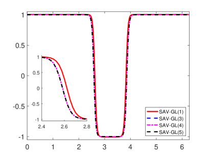
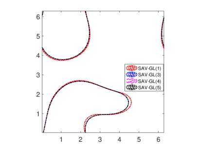
Figure 6.1: Example 6.2. Cut lines of $u(x,y,t)$ along $y=\frac{\pi}{2}$ (Left) and contour lines of $u(x,y,t)=-0.1$ (Right) at $t=200$.

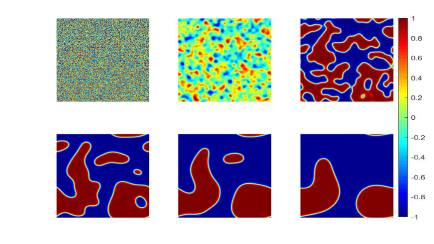
Figure 6.2: Example 6.2. Snapshots of the numerical solutions at $t=0,2,10,50,100$ and $200$ obtained by using SAV-GL(5) with $\tau=0.1$.

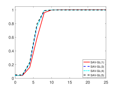
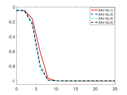
Figure 6.3: Example 6.2. Maximal and minimal values (from left to right) of the numerical solutions derived by SAV-GL(1), SAV-GL(3), SAV-GL(4) and SAV-GL(5) with $\tau=0.1$.

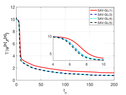
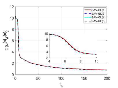
Figure 6.4: Example 6.2. Discrete energies of SAV-GL(1), SAV-GL(3), SAV-GL(4) and SAV-GL(5) with $\tau=0.1$ (Left) and $0.01$ (Right).

6.2 Cahn-Hilliard model

The Cahn-Hilliard (CH) model was introduced by Cahn and Hilliard in [13] to describe the complicated phase separation and coarsening phenomena. Different from the Allen-Cahn (6.1), the CH model is derived from the $H^{-1}$ gradient flow of the free energy (6.2) and is a fourth-order nonlinear PDE as follows

$$\frac{\partial u}{\partial t}=\Delta\left(-\epsilon^{2}\Delta u+u^{3}-u\right),$$ (6.3)

In order to validate the energy stability and accuracy of SAV-GL(1)$\sim$SAV-GL(6) for the CH model (6.3), the operators $\mathcal{L}$, $\mathcal{G}$ and the energy $\mathcal{F}_{1}(u)$ are taken as

$$\mathcal{L}=-\epsilon^{2}\Delta+\beta,~{}~{}~{}\mathcal{G}=\Delta,~{}~{}~{}\mathcal{F}_{1}(u)=\int_{\Omega}\frac{1}{4}\left(u^{2}-1\right)^{2}-\frac{\beta}{2}u^{2}dx,$$

where the parameter $\beta$ is chosen as $2$ in subsequent simulations, and it is obvious that the energy $\mathcal{F}_{1}(u)$ is bounded from below.

Example 6.3.

This example is used to test the accuracy of SAV-GL(1)$\sim$SAV-GL(6) for the CH model (6.3). The parameter $\epsilon$ is chosen as $1$, the initial data are $u(x,y,0)=0.4\sin(x)\sin(y)$, and SAV-GL(6) with $\tau=10^{-4}$ is used to generate the reference solution for computing the $L^{2}$ errors. Table 6.2 lists the $L^{2}$ errors of SAV-GL(1)$\sim$SAV-GL(6) at $t=0.3$ and corresponding convergence rates with different time stepsizes. One can find that the numerical accuracies of SAV-GL(1)$\sim$SAV-GL(4) are consistent with the theoretical, while SAV-GL(5) (resp. SAV-GL(6)) with the number of extrapolation points $\nu=3$ (resp. $\nu=4$) can arrive at the third-order (resp. fourth-order) accuracy, which validates the statement in Remark 4.6.

Table 6.2: Example 6.3. $L^{2}$ errors of SAV-GL(1)$\sim$SAV-GL(6) at $t=0.3$ and corresponding convergence rates.

	SAV-GL(1)		SAV-GL(2)		SAV-GL(3)
$K$	Errors	Orders	Errors	Orders	Errors	Orders
$120$	3.6925e-03	–	3.1250e-05	–	4.1560e-05	–
$160$	2.7695e-03	0.9998	1.7598e-05	1.9961	2.3339e-05	2.0057
$200$	2.2157e-03	0.9998	1.1270e-05	1.9969	1.4923e-05	2.0042
$240$	1.8465e-03	0.9999	7.8304e-06	1.9974	1.0357e-05	2.0034
$280$	1.5827e-03	0.9999	5.7548e-06	1.9978	7.6059e-06	2.0028
	SAV-GL(4)		SAV-GL(5)		SAV-GL(6)
$K$	Errors	Orders	Errors	Orders	Errors	Orders
$120$	2.2516e-05	–	1.8203e-09	–	2.4250e-09	–
$160$	1.2680e-05	1.9959	7.7214e-10	2.9811	7.2844e-10	4.1806
$200$	8.1207e-06	1.9969	3.9652e-10	2.9866	2.8832e-10	4.1535
$240$	5.6420e-06	1.9975	2.2981e-10	2.9919	1.3615e-10	4.1153
$280$	4.1465e-06	1.9979	1.4486e-10	2.9935	7.2146e-11	4.1198

Example 6.4.

This example applies SAV-GL(1)$\sim$SAV-GL(6) to a benchmark problem of studying the coarsening effect. The parameter $\epsilon$ in (6.3) is taken as $0.1$, the time stepsize $\tau$ is chosen as $0.1$ or $0.01$, and the initial data are specified by the following expression [77]

$$u_{0}(x,y,0)=\sum_{i=1}^{2}-\tanh\left(\frac{\sqrt{(x-x_{i})^{2}+(y-y_{i})^{2}-\nu_{i}}}{1.2\epsilon}\right)+1,$$

where $(x_{1},y_{1},\nu_{1})=(\pi-0.7,\pi-0.6,1.5)$ and $(x_{2},y_{2},\nu_{2})=(\pi+1.65,\pi+1.6,0.7)$.

Figure 6.6 gives the snapshos of the numerical solutions at $t=0,2,5,7,9$ and $20$ obtained by SAV-GL(5) with $\tau=0.01$. One can clearly observe the coarsening effect that the small circle is absorbed into the big circle, and the total absorption happens at around $t=10$. Figure 6.5 presents the cut lines and contour lines of the numerical solutions at $t=5$ and $20$ derived by SAV-GL(1), SAV-GL(3), SAV-GL(4) and SAV-GL(5) with $\tau=0.1$. It can be seen that those solutions at $t=5$ have some visible differences, see Figure 6.5 (a), but they become quite similar when $t=20$, see Figure 6.5 (b). Compared to the initial total mass, the total mass differences at $t_{n}$ obtained by SAV-GL(1), SAV-GL(3), SAV-GL(4) and SAV-GL(5) with $\tau=0.1$ are given in Figure 6.7, which checks the mass conservation numerically. Figure 6.8 shows the discrete energy curves of SAV-GL(1), SAV-GL(3), SAV-GL(4) and SAV-GL(5) with $\tau=0.1$ and $0.01$. One can see that the discrete energy curves are monotonically decreasing so that those schemes are energy stable in solving the CH model (6.3); the discrete energy curves of those schemes have big differences when $\tau=0.1$, but the differences become small for $\tau=0.01$; and similarly, SAV-GL(5) can obtain the steady state faster than t SAV-GL(1), SAV-GL(3) and SAV-GL(4). The results shown in Figure 6.8 are also consistent with the differences between the numerical solutions at $t=5$ in Figure 6.5.

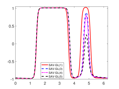
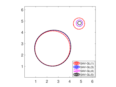
(a) $t=5$

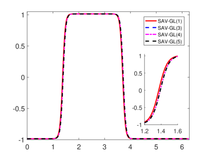
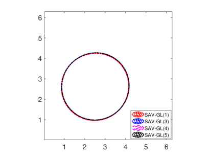
(b) $t=20$

Figure 6.5: Example 6.4. Left: cut lines of the numerical solutions along $y=x$; right: contour lines of $u(x,y,t)=-0.1$.

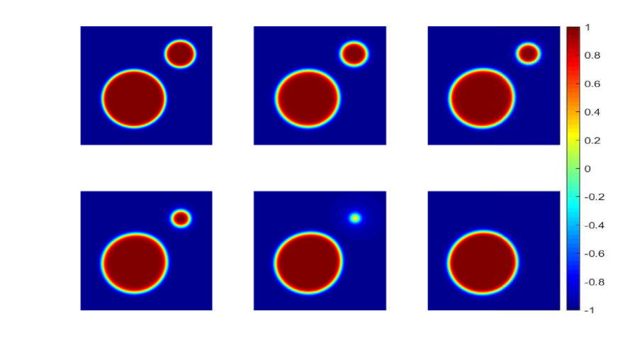
Figure 6.6: Example 6.4. Snapshots of the numerical solutions at $t=0,2,5,7,9$ and $20$ derived by using SAV-GL(5) with $\tau=0.1$.

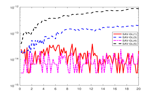
Figure 6.7: Example 6.4. Total mass differences of SAV-GL(1), SAV-GL(3), SAV-GL(4) and SAV-GL(5) with $\tau=0.1$.

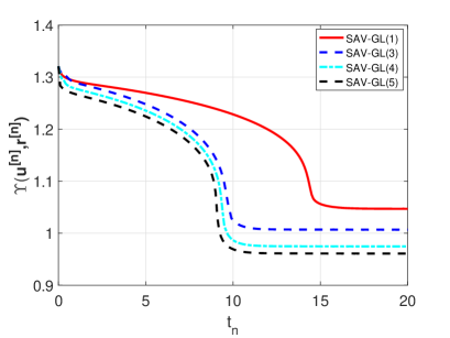
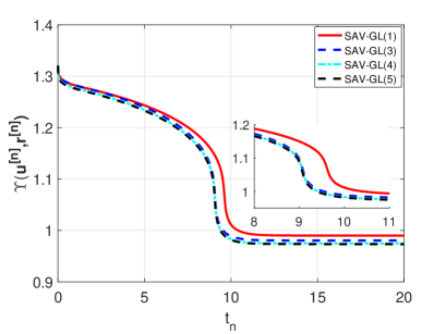
Figure 6.8: Example 6.4. Discrete energies of SAV-GL(1), SAV-GL(3), SAV-GL(4) and SAV-GL(5) with $\tau=0.1$ (Left) and $0.01$ (Right).

6.3 Phase field crystal model

The phase field crystal (PFC) model is a sixth-order nonlinear PDE

$$\frac{\partial u}{\partial t}=\Delta\mu,~{}~{}~{}\mu=u^{3}-\epsilon_{1}u^{2}+(1-\epsilon_{2})u+2\Delta u+\Delta^{2}u,$$ (6.4)

which can be derived from the $H^{-1}$ gradient flow of the following free energy

$$\mathcal{F}(u)=\int_{\Omega}\left[\frac{1}{4}u^{4}-\frac{\epsilon_{1}}{3}u^{3}+\frac{1-\epsilon_{2}}{2}u^{2}-|\nabla u|^{2}+\frac{1}{2}(\Delta u)^{2}\right]dx,$$

where $\epsilon_{1}$ and $\epsilon_{2}$ are two non-negative constants. This model can be used to describe many crystal phenomena such as edge dislocations [6], deformation and plasticity in nanocrystalline material [61], fcc ordering [70], epitaxial growth and zone refinement [25]. When $\epsilon_{1}=0$, (6.4) becomes the classical PFC equation.

In order to apply the SAV-GL schemes for the PFC equation successfully, the operators $\mathcal{L}$, $\mathcal{G}$ and the energy $\mathcal{F}_{1}(u)$ are chosen as

$$\mathcal{L}=\alpha\Delta^{2}+\beta,~{}~{}\mathcal{G}=\Delta,~{}~{}\mathcal{F}_{1}(u)=\int_{\Omega}\left[\frac{1}{4}u^{4}-\frac{\epsilon_{1}}{3}u^{3}+\frac{1\!-\!\epsilon_{2}\!-\!\beta}{2}u^{2}-|\nabla u|^{2}+\frac{1\!-\!\alpha}{2}(\Delta u)^{2}\right]dx,$$

where $0<\alpha<1$ and $\beta\geq 0$ are two given parameters. It can be verified that $\mathcal{F}_{1}(u)$ is bounded from below, since

$$\mathcal{F}_{1}(u)=\; \int_{\Omega}\left[\frac{1}{4}u^{4}-\frac{\epsilon_{1}}{3}u^{3}+\frac{1\!-\!\epsilon_{2}\!-\!\beta}{2}u^{2}+u\Delta u+\frac{1\!-\!\alpha}{2}(\Delta u)^{2}\right]dx$$

$$\geq\; \int_{\Omega}\left[\frac{1}{4}u^{4}-\frac{\epsilon_{1}}{3}u^{3}+\frac{1\!-\!\epsilon_{2}\!-\!\beta}{2}u^{2}-\frac{1}{2(1\!-\!\alpha)}u^{2}\right]dx,$$

where the inequality $ab\geq-\frac{1}{2\varepsilon}a^{2}-\frac{\varepsilon}{2}b^{2}$, $\varepsilon>0$ is used. Let us apply SAV-GL(1)$\sim$SAV-GL(6) to the PFC model (6.4) in order to validate the energy stability and accuracy.

Example 6.5.

This example checks the accuracy of SAV-GL(1)$\sim$SAV-GL(6) for the PFC model (6.4). The parameters are taken as $\epsilon_{1}=0$, $\epsilon_{2}=0.5$, $\alpha=0.99$ and $\beta=4$, the initial data are $u(x,y,0)=0.4\sin(x)\cos(y)$, and SAV-GL(6) with $\tau=5\times 10^{-5}$ is used to generate the reference solution for computing the $L^{2}$ errors. Table 6.3 shows the $L^{2}$ errors of SAV-GL(1)$\sim$SAV-GL(6) at $t=0.1$ and corresponding convergence rates with different time stepsizes. It is seen that the numerical accuracies of SAV-GL(1)$\sim$SAV-GL(4) are consistent with the theoretical, and SAV-GL(5) (resp. SAV-GL(6)) with the number of extrapolation points $\nu=3$ (resp. $\nu=4$) reaches the third-order (resp. fourth-order) accuracy for the PFC model (6.4), which validates the statement in Remark 4.6.

Table 6.3: Example 6.5. $L^{2}$ errors of SAV-GL(1)$\sim$SAV-GL(6) at $t=0.1$ and corresponding convergence rates.

	SAV-GL(1)		SAV-GL(2)		SAV-GL(3)
$K$	Errors	Orders	Errors	Orders	Errors	Orders
$240$	4.3324e-04	–	3.2234-06	–	4.7791e-06	–
$280$	3.7131e-04	1.0007	2.3687e-06	1.9987	3.5115e-06	1.9995
$320$	3.2487e-04	1.0006	1.8138e-06	1.9989	2.6887e-06	1.9995
$360$	2.8875e-04	1.0005	1.4333e-06	1.9990	2.1245e-06	1.9995
$400$	2.5987e-04	1.0005	1.1610e-06	1.9991	1.7209e-06	1.9995
	SAV-GL(4)		SAV-GL(5)		SAV-GL(6)
$K$	Errors	Orders	Errors	Orders	Errors	Orders
$240$	8.8351e-07	–	1.1427e-09	–	4.4513e-10	–
$280$	6.4931e-07	1.9980	7.1376e-10	3.0528	2.4953e-10	3.7546
$320$	4.9724e-07	1.9982	4.7372e-10	3.0700	1.4818e-10	3.9028
$360$	3.9296e-07	1.9984	3.2929e-10	3.0877	9.3183e-11	3.9384
$400$	3.1835e-07	1.9985	2.3740e-10	3.1055	6.1172e-11	3.9947

Example 6.6.

This example is used to simulate the polycrystal growth in a supercool liquid by solving (6.4). In this case, $\epsilon_{1}=0$, $\epsilon_{2}=0.25$, $\alpha=0.8$ and $\beta=0$, the spatial stepsize $h$ is $1$ for the domain $\Omega=[0,400]\times[0,400]$, and the time stepsize $\tau$ is taken as $0.1$ or $0.01$. The initial value $u_{0}$ is fixed to be a constant value $\phi_{0}=0.285$ firstly and then modified by setting three crystallites in three small square patches of the domain, where the centers of three crystallites are located at $(150,150),(200,250)$ and $(250,150)$, respectively, the length of each path is $40$, and the three crystallites are defined by the following expression (see e.g. [76, 52])

$$u(x_{l},y_{l})=\phi_{0}+B\left[\cos\left(\frac{\vartheta}{\sqrt{3}}y_{l}\right)\cos\left(\vartheta x_{l}\right)-\frac{1}{2}\cos\left(\frac{2\vartheta}{\sqrt{3}}y_{l}\right)\right],$$

with $B=0.446$, $\vartheta=0.66$, and local coordinates $x_{l},y_{l}$ given by

$$x_{l}(x,y)=x\sin(\theta)+y\cos(\theta),~{}~{}~{}y_{l}(x,y)=-x\cos(\theta)+y\sin(\theta),~{}~{}\mbox{for}~{}~{}\theta=\frac{\pi}{4},0,-\frac{\pi}{4}.$$

Figure 6.9 gives the cut lines and contour lines of the numerical solutions at $t=150$ derived by SAV-GL(1), SAV-GL(3), SAV-GL(4) and SAV-GL(5) with $\tau=0.1$, from which one can see that the numerical solutions computed by those schemes are quite similar. Figure 6.11 shows the differences between the total masses at $t_{n}$ and $t_{0}$ obtained by SAV-GL(1), SAV-GL(3), SAV-GL(4) and SAV-GL(5) with $\tau=0.1$, which checks the mass conservation numerically. Figure 6.10 gives the snapshots of the numerical solutions at $t=0,70,150,300,450$ and $1000$ computed by using SAV-GL(5) with $\tau=0.1$. It can be seen that the three different crystal grains grow and become large enough to form grain boundaries finally. Figure 6.12 displays the discrete energy curves of SAV-GL(1), SAV-GL(3) and SAV-GL(5) with $\tau=0.1$ and $0.01$, which indicates that those schemes are energy stable in solving the PFC model (6.4). The discrete energy curves of those schemes have some visible differences with $\tau=0.1$, but the differences are almost indistinguishable for $\tau=0.01$. It means that SAV-GL(5) may have some advantages to get the accurate steady solution of the PFC model (6.4) when a large time stepsize is taken.

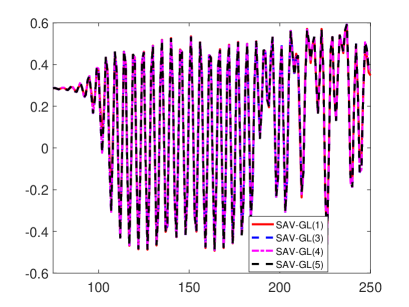
(a)

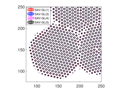
(b)

Figure 6.9: Example 6.6. Left: cut lines of the numerical solutions at $t=150$ along $y=x~{}(x\in[75,250])$; right: contour lines of $u=0.1$ at $t=150$.

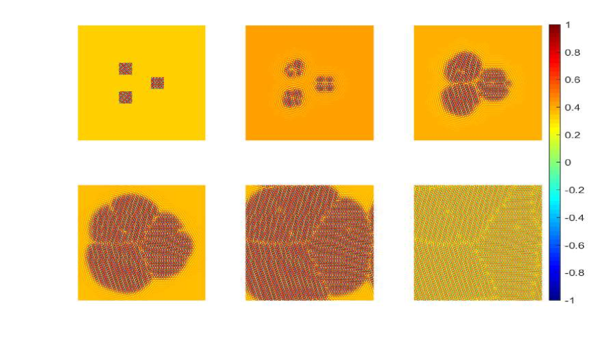
Figure 6.10: Example 6.6. Snapshots of the numerical solutions at $t=0,70,150,300,450$ and $1000$ computed by using SAV-GL(5) with $\tau=0.1$.

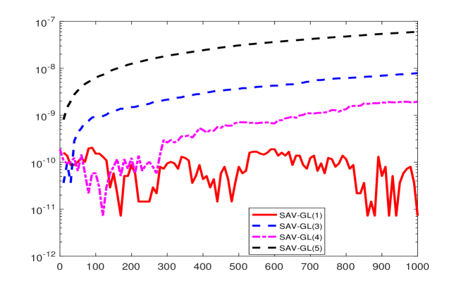
Figure 6.11: Example 6.6. Total mass differences of SAV-GL(1), SAV-GL(3), SAV-GL(4) and SAV-GL(5) with $\tau=0.1$.

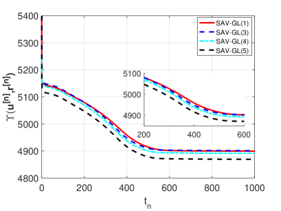
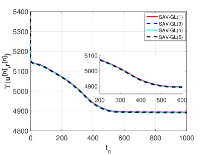
Figure 6.12: Example 6.6. Discrete energies of SAV-GL(1), SAV-GL(3), SAV-GL(4) and SAV-GL(5) with $\tau=0.1$ (Left) and $0.01$ (Right).

7 Conclusions

This paper proposed a general class of linear and unconditionally energy stable numerical schemes for the gradient flows by using the SAV and the general linear time discretizations (GLTDs). Those SAV-GL schemes could reach arbitrarily high-order accuracy in time, and only a coupled system of linear equations was solved at each time step since the nonlinear terms of the reformulated SAV equations were linearized based on extrapolation. Importantly, the resulting SAV-GL schemes contained most of the time integration schemes for the gradient flows in literature and many new schemes. The semi-discrete-in-time SAV-GL schemes were proved to be unconditionally energy stable when the GLTD was algebraically stable, and to be convergent with the order of $\min\{\hat{q},\nu\}$ under the diagonal stability and some suitable regularity and accurate starting values, where $\hat{q}$ was the generalized stage order of the GLTD and $\nu$ denoted the number of the extrapolation points in time. As two typical examples, the so-called one-leg and multistep Runge-Kutta (MRK) time integration schemes were considered for the gradient flows and their energy stabilities and error estimates were discussed separately. Because the proof of the energy stability was variational and the energy stability was available for the boundary conditions which made all boundary terms disappear when the integration by parts was performed, the above energy stability could be straightforwardly extended to the fully discrete SAV-GL schemes with the Galerkin finite element or the spectral methods or the finite difference methods, satisfying the summation by parts for the spatial discretization.

In order to demonstrate numerically the energy stability and accuracy of the SAV-GL schemes, the fully discrete SAV-GL schemes with the Fourier spectral spatial discretization were presented for three gradient flows equations (the Allen-Cahn, Cahn-Hilliard and phase field crystal models) with periodic boundary conditions. Our numerical experiments well demonstrated the theoretical results of SAV-GL(1)$\sim$SAV-GL(6) and also checked the discrete maximum principle for the Allen-Cahn model and the mass conservation for the Cahn-Hilliard and phase field crystal models. They also showed that the high-order SAV-GL schemes such as SAV-GL(5) might have some obvious advantage to derive the accurate steady solutions for the three gradient flow equations when taking a large time stepsize, and the SAV-GL scheme (3.10)-(3.11) with the integer $s\geq 2$ and the number of extrapolation points $\nu=s+1$ was convergent with the order of $s+1$.

Besides the one-leg and MRK time integration schemes considered in this paper, other time discretizations, such as the diagonally implicit multistage integrations (see e.g. [38, 11]) and the general class of two-step Runge-Kutta methods (see e.g. [21, 39]) etc., can be reformulated as the form of the GLTDs (2.2). Those methods may also possess good energy stability and accuracy for the gradient flows. In future, we will further address several interesting topics on numerical schemes for the gradient flows: exploring higher-order one-leg schemes with the aid of the novel SAV approach [36], estimating the errors of the fully discrete SAV-GL schemes, and combining the present SAV-GL schemes with the adaptive moving mesh method [81] for the mixture of two incompressible fluids etc.

References

- [1] G. Akrivis, B.Y. Li, and D.F. Li, Energy-decaying extrapolated RK-SAV methods for the Allen-Cahn and Cahn-Hilliard equations, SIAM J. Sci. Comput., 41(2019), A3703–A3727.
- [2] S.M. Allen and J.W. Cahn, A microscopic theory for antiphase boundary motion and its application to antiphase domain coarsening, Acta. Metall., 27(1979), 1085–1095.
- [3] D.M. Anderson, G.B. McFadden, and A.A. Wheeler, Diffuse-interface methods in fluid mechanics, Annu. Rev. Fluid Mech., 30(1998), 139–165.
- [4] S. Badia, F. Guilln-Gonzlez, and J.V. Gutirrez-Santacreu, Finite element approximation of nematic liquid crystal flows using a saddle-point structure, J. Comput. Phys., 230(2011), 1686–1706.
- [5] A. Baskaran, J.S. Lowengrub, C. Wang, and S.M. Wise, Convergence analysis of a second order convex splitting scheme for the modified phase field crystal equation, SIAM J. Numer. Anal., 51(2013), 2851–2873.
- [6] J. Berry, M. Grant, and K.R. Elder, Diffusive atomistic dynamics of edge dislocations in two dimensions, Phys. Rev. E, 73(2006), 031609.
- [7] W.J. Boettinger, J.A. Warren, C. Beckermann, and A. Karma, Phase-field simulation of solidification, Ann. Rev. Mater. Res., 32(2002), 163–194.
- [8] R.J. Braun and B.T. Murray, Adaptive phase-field computations of dendritic crystal growth, J. Cryst. Growth, 174(1997), 41–53.
- [9] K. Burrage and J.C. Butcher, Non-linear stability of a general class of differential equation methods, BIT, 20(1980), 185–203.
- [10] K. Burrage, High order algebraically stable multistep Runge-Kutta methods, SIAM J. Numer. Anal., 24(1987), 106–115.
- [11] J.C. Butcher, Diagonally-implicit multi-stage integration methods, Appl. Numer. Math., 11(1993), 347–363.
- [12] J.C. Butcher, General linear methods, Acta Numerica, 2006(2006), 157-256.
- [13] J.W. Cahn and J.E. Hilliard, Free energy of a nonunifotm ststem. I: Interfacial free energy, J. Chem. Phys., 28(1958), 258–267.
- [14] M. Calvo, J.I. Montijano, and S. Gonzalez-Pinto, On the existence of solution of stage equations in implicit Runge-Kutta methods, J. Comput. Appl. Math., 111(1999), 25–36.
- [15] L.Q. Chen, Phase-field models for microstructure evolution, Ann. Rev. Mater. Res., 32(2002), 113–140.
- [16] H.T. Cheng, J.J. Mao, and J. Shen, Optimal error estimates for the scalar auxiliary variable finite-element schemes for gradient flow, Numer. Math., 145(2020), 167–196.
- [17] Q. Cheng and J. Shen, Multiple scalar auxilary variable (MSAV) approach and its application to the phase-field vesicle membrane model, SIAM J. Sci. Comput., 40(2018), A3982–A4006.
- [18] Q. Cheng, J. Shen, and X.F. Yang, Highly efficient and accurate numerical schemes for the epitaxial thin film growth models by using the SAV approach, J. Sci. Comput., 78(2019), 1467–1487.
- [19] G. Dahlquist, Error analysis for a class of methods for stiff nonlinear initial value problems, in: G.A. Watson, Numerical Analysis, Lecture Notes in Mathematics, vol. 506, Springer, 1976, 60–72.
- [20] G. Dahlquist, -stability is equivalent to -stability, BIT, 18(1978), 384–401.
- [21] R. Dambrosio, G. Izzo, and Z. Jackiewicz, Search for highly stable two-step Runge-Kutta methods, Appl. Numer. Math., 62(2012), 1361–1379.
- [22] Q. Du, L.L. Ju, X. Li, and Z.H. Qiao, Maximum principle preserving exponential time differencing schemes for the nonlocal Allen-Cahn equation, SIAM J. Numer. Anal., 57(2019), 875–898,
- [23] C.M. Elliott and A.M. Stuart, The global dynamics of discrete semilinear parabolic equations, SIAM J. Numer. Anal., 30(1993), 1622–1663.
- [24] D.J. Eyre, Unconditionally gradient stable time marching the Cahn-Hilliard equation, Mater. Res. Soc. Symp. Proc., 529(1998), 39–46.
- [25] K.R. Elder, M. Katakowski, M. Haataja, and M. Grant, Modeling elasticity in crystal growth, Phys. Rev. Lett., 88(2002), 245701.
- [26] J. Fraaije, Dynamic density functional theory for microphase separation kinetics of block copolymer melts, J. Chem. Phys., 99(1993), 9202–9212.
- [27] J. Fraaije and G. Sevink, Model for pattern formation in polymer surfactant nanodroplets, Macromolecules, 36(2003), 7891–7893.
- [28] L. Golubovic, A. Levandovsky, and D. Moldovan, Interface dynamics and far-from-equilibrium phase transitions in multilayer epitaxial growth and erosion on crystal surfaces: Continumum theory insights, East Asian J. Appl. Math., 1(2011), 297–371.
- [29] Y. Gong, J. Zhao, and Q. Wang, Arbitrarily high-order unconditionally energy stable SAV schemes for gradient flow models, Comput. Phys. Commun., 249(2020), 107033.
- [30] F. Guilln-Gonzlez and G. Tierra, On linear schemes for a Cahn-Hilliard diffuse interface model, J. Comput. Phys., 234(2013), 140–171.
- [31] M.E. Gurtin, D. Polignone, and J. Vinals, Two-phase binary fluids and immiscible fluids described by an order parameter, Math. Models Meth. Appl. Sci., 6(1996), 815–831.
- [32] E. Hairer and G. Wanner, Solving Ordinary Differential Equations II: Stiff and Differential-Algebraic Problems, 2nd ed., Springer, New York, 1996.
- [33] E. Hairer and C. Lubich. Energy-diminishing integration of gradient systems, IMA J. Numer. Anal., 34(2014), 452-461.
- [34] D.M. Hou, M. Azaiez, and C.J. Xu, A variant of scalar auxiliary variable approaches for gradient flows, J. Comput. Phys., 395(2019), 307–332.
- [35] C.M. Huang, G.N. Chen, S.F. Li, and H.Y. Fu, -convergence of general linear methods for stiff delay differential equations, Comput. Math. Appl., 41(2001), 627–639.
- [36] F.K. Huang, J. Shen, and Z.G. Yang, A highly efficient and accurate new scalar auxiliary variable approach for gradient flows, SIAM J. Sci. Comput., 42(2020), A2514–A2536.
- [37] F.K. Huang and J. Shen, Implicit-explicit BDF SAV schemes for general dissipative systems and their error analysis, arXiv: 2103.06344, 2021.
- [38] G. Izzo and Z. Jackiewicz, Construction of algebraically stable DIMSIMs, J. Comput. Appl. Math., 261(2014), 72–84.
- [39] Z. Jackiewicz and S. Tracogna, A general class of two-step Runge-Kutta methods for ordinary differential equations, SIAM J. Numer. Anal., 32(1995), 1390–1427.
- [40] Z. Jackiewicz, General Linear Methods for Ordinary Differential Equations, John Wiley & Sons, Inc., 2009.
- [41] M.S. Jiang, Z.Y. Zhang, and J. Zhao, Improving the accuracy and consistency of the scalar auxiliary variable (SAV) method with relaxation, J. Comput. Phys., 456(2022), 110954.
- [42] A. Karma and W.J. Rappel, Phase-field method for computationally efficient modeling of solidification with arbitrary interface kinetics, Phys. Rev. E, 53(1996), R3017–R3020.
- [43] A. Karma and M. Plapp, Spiral surface growth without desorption, Phys. Rev. Lett., 81(1998), 4444.
- [44] R. Kobayashi, Modeling and numerical simulations of dendritic crystal growth, Phys. D, 63(1993) 410–423.
- [45] J.S. Kou, S.Y. Sun, and X.H. Wang, A novel energy factorization approach for the diffuse-interface model with Peng-Robinson equation of state, SIAM J. Sci. Comput., 42(2020), B30–B56.
- [46] B. Li and J.G. Liu, Thin film epitaxy with or without slope selection, Eur. J. Appl. Math., 14(2003), 713–743.
- [47] D. Li and Z.H. Qiao, On second order semi-implicit Fourier spectral methods for 2D Cahn-Hilliard equations, J. Sci. Comput., 70(2017), 301–341.
- [48] S.F. Li, Stability and -convergence of general linear methods, J. Comput. Appl. Math., 28(1989), 281–296.
- [49] S.F. Li, Stability and -convergence properties of multistep Runge-Kutta methods, Math. Comp., 69(1999), 1481–1504.
- [50] X.L. Li and J. Shen, Stability and error estimates of the SAV Fourier-spectral method for the phase field crystal equation, Adv. Comput. Math., 46(2020), 48.
- [51] Z.G. Liu and X.L. Li, The exponential scalar auxilary variable (E-SAV) approach for phase field models and its explicit computing, SIAM J. Sci. Comput., 42(2020), B630–B655.
- [52] Z.G. Liu and X.L. Li, A highly efficient and accurate exponential semi-implicit scalar auxiliary variable (ESI-SAV) approach for dissipative system, J. Comput. Phys., 447(2021), 110703.
- [53] N. Maurits and J. Fraaije, Mesoscopic dynamics of copolymer melts: From density dynamics to external potential dynamics using nonlocal kinetic coupling, J. Chem. Phys., 107(1997), 5879–5889.
- [54] J.T. Oden, A. Hawkins, and S. Prudhomme, General diffuse-interface theories and an approach to predictive tumor growth modeling, Math. Models Meth. Appl. Sci., 20(2010), 477–517.
- [55] J. Shen and X.F. Yang, A phase-field model and its numerical approximation for two-phase incompressible flows with different densities and viscosities, SIAM J. Sci. Comput., 32(2010), 1159–1179.
- [56] J. Shen and X.F. Yang, Numerical approximations of Allen-Cahn and Cahn-Hilliard equations, Dis. & Contin. Dyn. Sys., 28(2010), 1669–1691.
- [57] J. Shen, C. Wang, X.M. Wang, and S.M. Wise, Second-order convex splitting schemes for gradient flows with Ehrlich-Schwoebel type energy: Application to thin film epitaxy, SIAM J. Numer. Anal., 50(2012), 105–125.
- [58] J. Shen, J. Xu, and J. Yang, The scalar auxiliary variable (SAV) approach for gradient flows, J. Comput. Phys., 395(2018), 407–416.
- [59] J. Shen and J. Xu, Convergence and error analysis for the scalar auxiliary variable (SAV) schemes to gradient flows, SIAM J. Numer. Anal., 56(2018), 2895–2912.
- [60] J. Shen, J. Xu, and J. Yang, A new class of efficient and robust energy stable schemes for gradient flows, SIAM Rev., 61(2019), 474–506.
- [61] P. Stefanovic, M. Haataja, and N. Provatas, Phase field crystal study of deformation and plasticity in nanocrystalline materials, Phys. Rev. E, 80(2009), 046107.
- [62] C.J. Xu and T. Tang, Stability analysis of large time-stepping methods for epitaxial growth models, SIAM J. Numer. Anal., 44(2006), 1759–1779.
- [63] X. Tong, C. Beckermann, A. Karma, and Q. Li, Phase-field simulations of dendritic crystal growth in a forced flow, Phys. Rev. E, 63(2001), 061601.
- [64] L. Wang and H.J. Yu, On efficient second order stabilized semi-implicit schemes for the Cahn-Hilliard phase-field equation, J. Sci. Comput., 77(2018), 1185–1209.
- [65] S.L. Wang, R.F. Sekerka, A.A. Wheeler, B.T. Murray, S.R. Coriell, R.J. Braun, and G.B. McFadden, Thermodynamically-consistent phase-field models for solidification, Physica D, 69(1993), 189–200.
- [66] Y.U. Wang, Y.M. Jin, and A.G. Khachaturyan, Phase field microelasticity modeling of dislocation dynamics near free surface and in heteroepitaxial thin films, Acta Mater., 51(2003), 4209–4223.
- [67] X.Q. Wang, L.L. Ju, and Q. Du, Efficient and stable exponential time differencing Runge-Kutta methods for phase field elastic bending energy models, J. Comput. Phys., 316(2016), 21–38.
- [68] X.H. Wang, J.S. Kou, and J.C. Cai, Stabilized energy factorization approach for Allen-Cahn equation with logarithmic Flory-Huggins potential, J. Sci. Comput., 82(2020), 25.
- [69] S.M. Wise, J.S. Lowengrub, H.B. Frieboes, and V. Cristini, Three-dimensional multispecies nonlinear tumor growthi: model and numerical method, J. Theor. Biol., 253(2008), 524–543.
- [70] K.A. Wu, A. Adland, and A. Karma, Phase-field-crystal model for fcc ordering, Phys. Rev. E, 81(2010), 061601.
- [71] X. Wu, G.J. van Zwieten, and K.G. van der Zee, Stabilized second-order convex splitting schemes for Cahn-Hilliard models with application to diffuse-interface tumor-growth models, Int. J. Numer. Methods Biomed. Eng., 30(2014), 180–203.
- [72] J.X. Yang and J. Kim, A variant of stabilized-scalar auxiliary variable (S-SAV) approach for a modified phase-field surfactant model, Comput. Phys. Commun., 261(2021), 107825.
- [73] X.F. Yang, Linear, first and second-order, unconditionally energy stable numerical schemes for the phase field model of homopolymer blends, J. Comput. Phys., 327(2016), 294–316.
- [74] X.F. Yang, J. Zhao, Q. Wang, and J. Shen, Numerical approximations for a three components Cahn-Hilliard phase-field model based on the invariant energy quadratization method, Math. Models Meth. Appl. Sci., 27(2017), 1993–2030.
- [75] X.F. Yang and L.L. Ju, Efficient linear schemes with unconditional energy stability for the phase field elastic bending energy model, Comput. Meth. Appl. Mech. Eng., 315(2017), 691–712.
- [76] X.F. Yang and D.Z. Han, Linearly first- and second-order, unconditionally energy schemes for the phase field crystal model, J. Comput. Phys., 330(2017), 1116–1134.
- [77] X.F. Yang and G.D. Zhang, Convergence analysis for the invarint energy quadratization (IEQ) schemes for solving the Cahn-Hilliard and Allen-Cahn equations with general nonlinear potential, J. Sci. Comput., 82(2020), 55.
- [78] Z.G. Yang, L.L. Lin, and S.C. Dong, A family of second-order energy-stable schemes for Cahn-Hilliard type equations, J. Comput. Phys., 383(2019), 24–54.
- [79] P.T. Yue, J.J. Feng, C. Liu, and J. Shen, A diffuse-interface method for simulating two-phase flows of complex fluids, J. Fluid Mech., 515(2004), 293–317.
- [80] C.H. Zhang, J. Ouyang, C. Wang, and S.M. Wise, Numerical comparison of modified-energy stable SAV-type schemes and classical BDF methods on benchmark problems for the functionalized Cahn-Hilliard equation, J. Comput. Phys., 423(2020), 109772.
- [81] Z.R. Zhang and H.Z. Tang, An adaptive phase field method for the mixture of two incompressible fluids, Comput. & Fluids, 36(2007), 1307–1318.
- [82] Y.R. Zhang and J. Shen, A generalized SAV approach with relaxation for dissipative systems, arXiv: 2201.12587, 2022.