Nuclei instance segmentation and classification in histopathology images with StarDist

Abstract

Instance segmentation and classification of nuclei is an important task in computational pathology. We show that StarDist, a deep learning nuclei segmentation method originally developed for fluorescence microscopy, can be extended and successfully applied to histopathology images. This is substantiated by conducting experiments on the Lizard dataset, and through entering the Colon Nuclei Identification and Counting (CoNIC) challenge 2022, where our approach achieved the first spot on the leaderboard for the segmentation and classification task for both the preliminary and final test phase.

Index Terms—  image segmentation, challenge, deep learning, histopathology

1 Introduction

Reliably identifying individual cell nuclei in microscopy images is a ubiquitous task in the life sciences. This can be especially challenging when nuclei are densely packed together, which might cause commonly used bounding-box based detection methods (and also pixel grouping methods) to struggle. To address this problem, we – together with collaborators – introduced a deep learning based object detection and segmentation approach called StarDist [1, 2]. Instead of bounding boxes, StarDist represents objects with star-convex polygons, which are well suited for roundish objects such as cell nuclei. Being primarily developed for fluorescence microscopy, we here aim to investigate i) how StarDist can be extended to additionally perform classification of detected objects, ii) whether it can be successfully applied to the different domain of histopathology images, and iii) how it compares quantitatively against other methods used in histopathology (e.g. HoverNet [3]) as part of the Colon Nuclei Identification and Counting (CoNIC) challenge [4].

Input image	Ground truth	StarDist prediction

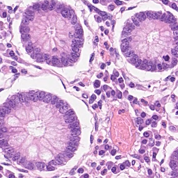
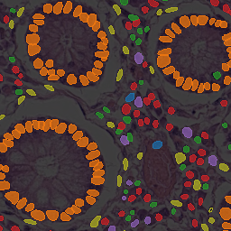
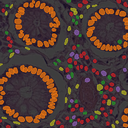
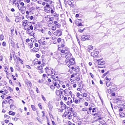
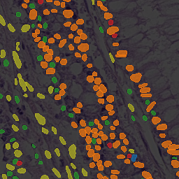
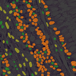
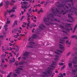
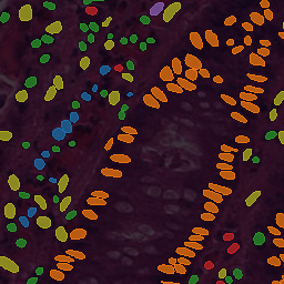
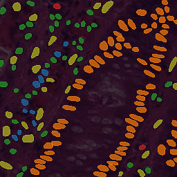
Fig. 1: Example input images from the CoNIC challenge dataset (left) with ground truth (middle) and StarDist predictions (right). Each nucleus instance is shown with a color that reflects its class (see legend at bottom).

In this paper, we describe our extension of StarDist to perform nuclei classification and discuss several important adjustments that we made for our submissions to the CoNIC challenge. We evaluate key parameters via ablation experiments on the public challenge data and by reviewing the results of our challenge submissions on the hidden preliminary and final test data. First, we find that besides typical geometric data augmentations, special color augmentations to address staining variabilities in hematoxylin (H) and eosin (E) are crucial to train models that generalize well to new data. Second, addressing the issue of imbalanced (cell) class distributions is decisive to achieve high scores for the metrics used by the CoNIC challenge, which assign equal importance to each cell type. Third, test-time augmentations and model ensembles do indeed substantially boost performance. Fourth, we find that a rather simple shape refinement procedure can additionally improve the segmentation quality of StarDist.

2 Method

2.1 Extending StarDist for nuclei classification

We shortly review the StarDist detection/segmentation approach as described in [1, 2]: First, a convolutional neural network (CNN) takes a single input image and for each pixel predicts 1) an object probability to know if it is part of an object, and 2) radial distances to the boundary of the object at that location (i.e. a star-convex polygon representation). Second, each pixel with an object probability above a chosen threshold votes for a polygon to represent the shape of the object it belongs to. Since a given object is potentially represented by many pixels which voted for its shape, a non-maximum suppression (NMS) step is performed to prune the redundant polygons that likely represent the same object.

The original StarDist [1, 2] approach only allows for the prediction of individual shapes of object instances. To additionally perform object instance classification, we extend StarDist by adding a semantic segmentation head to the CNN backbone (besides the existing two heads for object probabilities and radial distances). Now, the CNN additionally predicts 3) class probabilities for every pixel. After performing the object instance segmentation as described before, the class (i.e., cell type) of each object instance is determined by aggregating the class probabilities from all pixels that are part of the respective instance.

Please note that all of our improvements and extensions of StarDist (as compared to [1, 2]) are included in our public code repository. Additional code developed to create our challenge submissions will be made available after the challenge has ended.

2.2 Data

We only use the Lizard dataset [5] for training our models, specifically the extracted patches provided by the CoNIC challenge organizers. The dataset consists of $4981$ images of size $256\times 256\times 3$ and corresponding label masks for the nuclei of six different cell types/classes: neutrophil, epithelial, lymphocyte, plasma, eosinophil, and cells belonging to connective tissue. The distribution of cell classes is highly imbalanced: whereas epithelia nuclei constitute more than $60$% of all objects, neutrophil and eosinophil nuclei each represent less than $1$% of all instances. Of all provided images we use $90$% for training and $10$% as (internal) validation set. Besides dividing pixel values by $255$, we do not perform any image preprocessing or data cleaning.

2.3 Class balancing and augmentations

We investigate different strategies to address the severe imbalance of the distribution of nucleus types in the dataset. Concretely, we explore 1) applying class weights for the loss of the semantic segmentation head, 2) using a focal loss [6] for the semantic segmentation head, 3) and simple resampling/oversampling of the training data with a probability roughly proportional to the inverse of the class frequency (i.e., duplicating entire image patches that contain many nuclei of the minority classes). Somewhat surprisingly, we find that simple training data oversampling is by far the most effective strategy to combat class imbalance issues (Section 3.1).

Based on our own augmentation library Augmend, we apply common geometric augmentations (flips and $90$ degree rotations, elastic deformations) to each pair of input and label image on-the-fly during training. Additionally, we explore different types of pixel-wise color augmentations by randomly changing 1) brightness, 2) brightness and hue, or 3) brightness and H&E staining.

2.4 Model and Training details

We use a StarDist model with $64$ rays and a U-Net [7] backbone of depth $4$. For training, we apply a binary cross-entropy loss for the object probabilities, mean absolute error for the radial distances, and a sum of categorical cross-entropy and Tversky loss [8] for the class probabilities. Training was done from randomly initialized weights for $1000$ epochs ($256$ batches of size $4$) using the Adam [9] optimizer starting with a learning rate of $0.0003$, which was reduced by half if no progress was made for $80$ epochs. To reduce the effect of overfitting, we choose the weights for the final model that corresponded to the smallest validation loss during training.

2.5 Test-time augmentations (TTA)

Although data augmentation is heavily used during training, we find that test-time augmentations (TTA) still lead to improved results. To that end, we implement $8$ distinct geometric TTA and aggregate the respective predictions to obtain more robust results. Concretely, we apply all multiples of $90$ degree rotations (with and without horizontal flips) to the input image and collect the CNN predictions for object probabilities, radial distances, and class probabilities. Prediction tensors are merged by simple element-wise averaging.

Note that since the radial distances in StarDist refer to directions defined in polar coordinates, these geometric transformations of the input image will result in a permutation w.r.t. the order of the radial distances of the predicted tensor. For example, a $90$ degree rotation of the input will cyclically shift the order of the radial distances – which has to be accounted for before merging the tensors obtained via TTA.

2.6 Postprocessing and shape refinement

As mentioned in Section 2.1, non-maximum suppression (NMS) is applied as postprocessing after CNN prediction. Concretely, NMS is performed here based on a set of polygon candidates (those with object probability above a chosen threshold) obtained from the merged CNN predictions (see above). In each round of NMS, of the remaining polygons that haven’t been suppressed, the one with highest object probability is selected as the “winner” and will suppress all other polygons that sufficiently overlap. Instead of just keeping the winner polygon in each round to yield the final object instances – as is typically done in StarDist – we instead group each winner polygon together with all the polygons that it suppressed. For each group, we rasterize all polygons as binary masks and aggregate them by majority vote to obtain the mask of the given object instance. We refer to this procedure as shape refinement.

2.7 Model ensembles

We may additionally aggregate the predictions from a small number of separately trained StarDist models. To that end, we collect the CNN predictions from each model and merge them in the same way as described for TTA in Section 2.5. This approach makes it also trivial to combine model ensembling with TTA, by simply collecting and merging the TTA predictions from all models of the ensemble. If it is desired to reduce the ensemble’s computational requirements, we can randomly sample only a few augmentations per model (instead of using all $8$ possible geometric test-time augmentations). Note that postprocessing and shape refinement (Section 2.6) is only performed once for the entire ensemble.

3 Results

We adopt the metrics used by CoNIC (see [4] for definitions) to evaluate the instance segmentation and classification performance of our models. Concretely, the overall performance is measured via the multi-class panoptic quality [10]. The panoptic quality $\mathrm{PQ}$ is defined as the product of detection quality $\mathrm{DQ}$ ($F_{1}$ score, i.e. the harmonic mean of precision and recall) and segmentation quality $\mathrm{SQ}$ (average intersection over union of all correct matches). The multi-class panoptic quality $\mathrm{mPQ}=\tfrac{1}{T}\sum_{t=1}^{T}\mathrm{PQ}_{t}$ is then defined as the average of the panoptic qualities $\mathrm{PQ}_{t}$ (only considering object instances of predicted class $t$) for all $T$ cell classes/types.

3.1 Ablation experiments

To investigate the effects of different a) class balancing approaches, b) color augmentations, and c) test-time strategies, we show the results of several ablation experiments on the internal validation dataset in Table 1. Regarding class balancing, we find somewhat surprisingly that simple oversampling yields by far the best results for all metrics. For color augmentations, our experiments seem to indicate that simple brightness augmentations are much more effective than augmentations that also affect hue or H&E staining. This might be explained by the strong similarity between the internal training and validation data. However, our observations are notably different regarding the results of our challenge submissions, where staining augmentations lead to considerably improved performance (cf. Table 2). This might be due to a more pronounced domain shift of the external preliminary test data. Finally, test-time augmentations and shape refinement lead to smaller improvements (relative to class balancing and color augmentations).

	$\mathrm{mPQ}$	$\mathrm{PQ}$	$\mathrm{DQ}$	$\mathrm{SQ}$
a) class balancing
none	0.3900	0.6841	0.4730	0.5510
focal loss	0.4541	0.6711	0.5679	0.7882
class weights	0.5099	0.6896	0.6281	0.8059
oversampling	0.5885	0.6987	0.7186	0.8187
b) color augmentation
brightness	0.6034	0.7037	0.7342	0.8218
brightness + hue	0.5495	0.6850	0.6790	0.8074
brightness + H&E	0.5884	0.6987	0.7186	0.8187
c) test-time strategy
shape refinement	0.5832	0.6980	0.7053	0.8264
TTA	0.5913	0.6980	0.7212	0.8192
TTA + shape ref.	0.5984	0.7047	0.7225	0.8276
none	0.5884	0.6987	0.7186	0.8187

Table 1: Ablation results on the internal validation set.

Preliminary test leaderboard (Task 1: segmentation and classification)
Model	Strategy	Pos.	$\mathrm{mPQ}^{+}$	$\mathrm{PQ}$	$\mathrm{PQ}^{+}$	$\mathrm{PQ}^{+}_{pla}$	$\mathrm{PQ}^{+}_{neu}$	$\mathrm{PQ}^{+}_{epi}$	$\mathrm{PQ}^{+}_{lym}$	$\mathrm{PQ}^{+}_{eos}$	$\mathrm{PQ}^{+}_{con}$
$A$	basic	76	0.3647	0.5805	0.5822	0.3750	0.0877	0.5590	0.4391	0.3349	0.3929
$B$	+ H&E staining augment	30	0.4343	0.6380	0.6344	0.5029	0.1380	0.6265	0.4449	0.4652	0.4283
$\phantom{{}_{2}}B_{2}$	+ TTA	19	0.4515	0.6473	0.6452	0.5190	0.1639	0.6190	0.4614	0.5266	0.4188
$\phantom{{}_{3}}B_{3}$	+ shape refinement	13	0.4583	0.6529	0.6512	0.5207	0.1812	0.6230	0.4711	0.5331	0.4205
$C$	+ oversampling	2	0.4970	0.6650	0.6625	0.5039	0.3407	0.6432	0.4748	0.5479	0.4715
$B,C,D$	+ ensemble	1	0.4971	0.6706	0.6669	0.5277	0.2819	0.6565	0.4887	0.5533	0.4745
Final test leaderboard (Task 1: segmentation and classification)
$C,D,E,F$	as above	1	0.5013	0.6607	0.6555	–	–	–	–	–	–

Table 2: Preliminary and final test leaderboard results for submissions of our team EPFL | StarDist for the nuclear segmentation and classification task of the CoNIC challenge. Pos. denotes position at the end of the preliminary/final test phase.

3.2 CoNIC preliminary and final test phase submissions

The CoNIC challenge consists of two tasks: 1) nuclear segmentation and classification and 2) prediction of cellular composition (i.e., per-class nuclei counts). As our aim is to improve StarDist, we focused on the first task and used the obtained results for task 2 by simply reporting the number of segmented nuclei per class. The preliminary test phase allowed each team to make a limited number of submissions, which were quantitatively evaluated on a fraction of the final test set and the results shown publicly on a preliminary test leaderboard. For the final test phase only a single submission per team was allowed with the results on the complete test set being available on a final test leaderboard.

Table 2 reports the results of our team EPFL | StarDist for selected submissions on the preliminary test leaderboard as well for the final test leaderborard. For the preliminary test phase, we first trained a basic StarDist model ($A$) with only standard geometric augmentations and class balancing via weighted loss terms. As we suspected a considerable domain shift in the test data, we next added heavy H&E staining augmentations ($B$) that resulted in a large performance increase. Without training a new model, we then added test-time augmentations ($B_{2}$) and shape refinement ($B_{3}$), each resulting in noticeable performance gains. We finally realized that further addressing the class imbalance was likely to be the largest contributing factor to increase performance and thus aggressively oversampled the minority classes in the training data, leading to substantially improved results ($C$). Finally, we similarly trained another model $D$ and submitted an ensemble of three models ($B$–$D$), yielding a slight improvement and resulting in the first place on the concluding preliminary test leaderboard. For the final test set, we submitted an ensemble of four models ($C$–$F$), thereby combining two well performing models from the preliminary phase and two newly trained models $E$ and $F$, resulting in the top spot on the final test leaderboard of the CoNIC challenge.

4 Discussion

We described how StarDist can be successfully used and extended for object instance segmentation and classification in the context of histopathology. Overall, our approach is competitive for the segmentation and classification task of the CoNIC challenge, which is demonstrated by winning the preliminary and final test phase.

5 Compliance with ethical standards

No ethical approval was required for this study.

6 Acknowledgments

M.W. is supported by the EPFL School of Life Sciences and a generous foundation represented by CARIGEST SA.

References

- [1] Uwe Schmidt, Martin Weigert, Coleman Broaddus, and Gene Myers, “Cell detection with star-convex polygons,” in MICCAI, 2018.
- [2] Martin Weigert, Uwe Schmidt, Robert Haase, Ko Sugawara, and Gene Myers, “Star-convex polyhedra for 3D object detection and segmentation in microscopy,” in WACV, 2020.
- [3] Simon Graham, Quoc Dang Vu, Shan E Ahmed Raza, Ayesha Azam, Yee Wah Tsang, Jin Tae Kwak, et al., “Hover-net: Simultaneous segmentation and classification of nuclei in multi-tissue histology images,” Medical Image Analysis, vol. 58, pp. 101563, 2019.
- [4] Simon Graham, Mostafa Jahanifar, Quoc Dang Vu, Giorgos Hadjigeorghiou, Thomas Leech, David Snead, et al., “CoNIC: Colon nuclei identification and counting challenge 2022,” arXiv:2111.14485, 2021.
- [5] Simon Graham, Mostafa Jahanifar, Ayesha Azam, Mohammed Nimir, Yee-Wah Tsang, Katherine Dodd, Emily Hero, et al., “Lizard: A large-scale dataset for colonic nuclear instance segmentation and classification,” in ICCV Workshops, October 2021.
- [6] Tsung-Yi Lin, Priya Goyal, Ross B. Girshick, Kaiming He, and Piotr Dollár, “Focal loss for dense object detection,” in ICCV, 2017.
- [7] Olaf Ronneberger, Philipp Fischer, and Thomas Brox, “U-Net: Convolutional networks for biomedical image segmentation,” in MICCAI, 2015.
- [8] Nabila Abraham and Naimul Mefraz Khan, “A novel focal Tversky loss function with improved attention U-net for lesion segmentation,” in ISBI, 2019.
- [9] Diederik Kingma and Jimmy Ba, “Adam: A method for stochastic optimization,” ICLR, 2015.
- [10] Alexander Kirillov, Kaiming He, Ross Girshick, Carsten Rother, and Piotr Dollár, “Panoptic segmentation,” in CVPR, 2019.