Improving Ant Colony Optimization Efficiency for Solving Large TSP Instances

Abstract

Ant Colony Optimization (ACO) is a family of nature-inspired metaheuristics often applied to finding approximate solutions to difficult optimization problems. Despite being significantly faster than exact methods, the ACOs can still be prohibitively slow, especially if compared to basic problem-specific heuristics. As recent research has shown, it is possible to significantly improve the performance through algorithm refinements and careful parallel implementation benefiting from multi-core CPUs and dedicated accelerators. In this paper, we present a novel ACO variant, namely the Focused ACO (FACO). One of the core elements of the FACO is a mechanism for controlling the number of differences between a newly constructed and a selected previous solution. The mechanism results in a more focused search process, allowing to find improvements while preserving the quality of the existing solution. An additional benefit is a more efficient integration with a problem-specific local search. Computational study based on a range of the Traveling Salesman Problem instances shows that the FACO outperforms the state-of-the-art ACOs when solving large TSP instances. Specifically, the FACO required less than an hour of an 8-core commodity CPU time to find high-quality solutions (within 1% from the best-known results) for TSP Art Instances ranging from 100 000 to 200 000 nodes.

1 Introduction

Ant Colony Optimization (ACO) belongs to a growing collection of nature-inspired metaheuristics that can be applied to solve various optimization problems [14, 45]. Heuristics, in general, do not guarantee to find an optimum but can be helpful if the available computational budget is insufficient to use an exact algorithm. Typically, this is the case if one considers solving NP-hard combinatorial optimization problems (COPs). For example, even though the Traveling Salesman Problem (TSP) is one of the most thoroughly studied COPs, still, to date, the largest solved to optimality instance of the problem has only 85 900 cities and the computations took years of CPU time [1].

In general, the ACO refers not to a single algorithm but rather to a family of algorithms whose main principles mimic the behavior of certain species of ants [16]. Among the most well-known ACOs are the Ant System [10], Ant Colony Sytem [15], MAX-MIN Ant System (MMAS) [41], Population-based ACO [20], and Beam ACO [31]. Since the first application of the Ant System to solve the TSP [10], researchers have proposed numerous applications of the ACOs including, among others, vehicle routing [3], the set cover problem [28], edge detection on digital images [34], protein folding [37], and scheduling problems [13]. The main motivations behind developing multiple ACO variants include adaptation to new types of problems, improvements to the convergence to high-quality solutions, and more efficient utilization of computing resources. Additionally, some work was motivated by the ever-growing computational power offered by multi-core CPUs [36, 47], specialized accelerators [33, 44], and general-purpose graphics processing units (GPUs) [6, 12, 39, 40]. More computational power allowed not only to reduce the computation time but also to tackle larger problems [8, 35].

In this paper, building upon novel ideas and recent research on applying the ACO to large TSP instances, we propose a new algorithm loosely based on the MMAS. The algorithm, named the Focused ACO (FACO), can be used to find high-quality solutions (within 1% from the best-known results) to the TSP instances with more than one hundred thousand nodes while also being competitive in terms of the computation time. Our straightforward parallel implementation of the algorithm requires less than an hour to solve (approximately) the TSP instances from the TSP Art Instances dataset [11] with $10^{5}$ (100k) to $2\cdot 10^{5}$ (200k) cities when executing on a computer with an 8-core commodity CPU. The main contributions presented in this paper can be summarized as follows:

• We present a novel ACO algorithm named the FACO, which contains a mechanism for controlling the differences between the newly constructed solutions and a selected previous solution. The resulting search process is more narrow (focused), allowing to find improvements to small parts of the existing solution without worsening the quality of the rest.

• We show how the control over the new components (differences) in the constructed solutions can be used to guide the local search (LS) heuristic (2-opt) in order to reduce its computation time.

• We show how the proposed ideas can be applied along the recent advancements presented in the literature on applying the ACO to tackle large TSP instances efficiently.

• We present a sensitivity analysis of the proposed FACO algorithm considering both the quality of the results and the computation time. In particular, we show how the number of new components in the constructed solutions affects the efficiency of the algorithm.

• We describe our parallel implementation of the FACO for shared-memory multiprocessing. The implementation allows to efficiently utilize the processing power of a multicore CPU.

• We present an extensive computational study of the proposed algorithm and compare its efficiency to that of the recently proposed ACOs, and also with the powerful LKH solver by Helsgaun [21] on the TSP instances with up to two hundred thousand cities (nodes).

The remainder of this paper is organized as follows. In Sec. 2 we describe the MMAS, which is the basis for the proposed FACO, and highlight the main performance obstacles of the ACOs, including the MMAS. Section 3 contains a summary of the recent research focused on improving the performance of the ACOs. In Sec. 4 we detail the proposed FACO, emphasizing features that are essential for the good performance when solving large TSP instances. Section 5 summarizes the experimental study of the FACO, which comprised a sensitivity analysis of its main parameters and a comparison with the state-of-the-art ACOs. Finally, Sec. 6 summarizes the work.

2 Background

2.1 Ant Colony Optimization

The ACO belongs to a group of swarm-based metaheuristics (SBMs) in which a number of simple information-processing units (agents) construct solutions to an optimization problem. The agents can often interact with each other, often indirectly, to improve the problem-solving efficiency [27]. Typically, the SBMs mimic some biological systems, including ant colonies, flocks of birds, and schools of fish, among others [18].

The TSP was among the first combinatorial optimization problems to which the ACO was applied [17], and still to date remains a default choice when describing and verifying the efficiency of new variants of the ACO [8, 26, 41]. Typically, the TSP is modeled using a complete graph $G=(V,E)$ in which a set of nodes $V$ corresponds to a set of cities or locations on a map, and a set of edges $E$ represents direct connections or roads between pairs of the nodes. For convenience, the nodes can be numbered from 0 to $n-1$ ($n$ being the number of nodes), and the set of edges (arcs) can be defined as $E=\{(i,j):i,j\in V,i\neq j\}$, i.e., each edge is represented using a pair of nodes. The TSP typically corresponds to a symmetric variant in which the order of the edges‘ nodes is not important. Complementary, if the edges are directed, then the problem is asymmetric (ATSP). With every edge, $(i,j)$, a positive cost, $d_{ij}$, is associated, allowing to model real-world distances or travel costs between cities $i$ and $j$. The ATSP variant allows the costs to differ depending on the direction of travel. Solving the (A)TSP requires finding a minimum cost route visiting each city exactly once, or, in other words, the minimum cost Hamiltonian cycle in graph $G$.

In the ACO, a virtual ant travels through the graph $G$ moving from a current node to one of the neighbor nodes. The route of the ant becomes its solution. The decision of which node to choose next is based on the costs of the edges leading to yet unvisited nodes and additional information in the form of so-called pheromone trails deposited on the edges. Specifically, for every edge $(i,j)\in E$ a pheromone trail, $\tau_{ij}(t)$, is defined, where $t$ denotes discrete time. The use of the artificial pheromone trails mimics how some species of ants use chemical substances as a medium of indirect communication between the individuals [16]. The values (concentrations) of the artificial pheromone trails are stored in the computer‘s memory as a real-valued matrix of size $O(n^{2})$. The matrix is often referred to as a pheromone memory. Some variants of the ACO, including the MMAS, impose bounds on the pheromone values, i.e., $\tau_{\rm min}$ and $\tau_{\rm max}$, which gives more control over the exploration–exploitation behavior induced by the pheromone

Focusing on the MMAS, which is the basis of the proposed FACO algorithm, the solution construction process of the ACOs can be explained in more detail as follows. Ant $k$ located at node $i$ selects edge $(i,j)$ with the probability defined as:

$$p_{ij}^{k}(t)=\frac{[\tau_{ij}(t)]^{\alpha}[\eta_{ij}]^{\beta}}{\sum_{l\in\mathcal{N}_{i}^{k}}[\tau_{il}(t)]^{\alpha}[\eta_{il}]^{\beta}}\;\quad\textrm{if}\;j\in\mathcal{N}_{i}^{k}\,,$$ (1)

where $\tau_{ij}(t)$ is the value of the pheromone trail deposited on edge $(i,j)$; $\eta_{ij}$ is the value of so-called heuristic information of edge $(i,j)$; $\alpha$ and $\beta$ are parameters that control the relative influence of the pheromone values and the heuristic information, respectively. Finally, $\mathcal{N}_{i}^{k}$, is a set of nodes (that neighbor $i$) to be visited by ant $k$. In the case of the TSP, the value of the heuristic information of edge $(i,j)$ is defined as a reciprocal of the edge length (cost), i.e., $\frac{1}{d_{ij}}$, what makes the edge more attractive the shorter it is.

In the case of the TSP, the heuristic information remains static as the distances between the cities do not change. However, the pheromone memory is dynamic, i.e., the amount of pheromone can diminish due to a process called evaporation, or can increase to make it more likely for an edge to be selected by the ants in subsequent iterations. Increasing the amount of pheromone aims at inducing a positive feedback loop resulting in new solutions similar to the best solutions found so far but with a lower cost. In contrast, evaporating the pheromone increases the chance of building solutions with more differences and possibly escaping from a local minimum in the solution search space. In other words, the pheromone deposition and evaporation allow to balance between exploitation and exploration, respectively [17, 41].

In the MMAS, the pheromone values are initialized to a maximum value, $\tau_{\rm max}(0)$. Next, the main loop of the algorithm starts. Firstly, all ants construct their solutions to the problem. Next, the evaporation process lowers the values of all pheromone trails according to a predefined parameter $\rho$ but not below $\tau_{\rm min}(t)$, where $t$ denotes the current iteration. Finally, the pheromone deposition adds a small amount of pheromone to the edges belonging to a high quality solution, which is either the best solution found in the current iteration (iteration best solution) or the best solution found to date (global best solution). Precisely, the amount of pheromone on edge $(i,j)$ changes between the current, $t$, and next, $t+1$, iteration according to equation:

$$\tau_{ij}(t+1)=\textrm{max}\left\{\tau_{\rm min}(t+1),\textrm{min}\left\{\tau_{\rm max}(t+1),\rho\tau_{ij}(t)+\Delta\tau_{ij}(t)\right\}\right\}\,,$$ (2)

where $\rho\in{[}0,1{]}$ is a parameter controlling the amount of the pheromone that remains after the evaporation and $\Delta\tau_{ij}(t)$ is the amount of pheromone deposited on the edge $(i,j)$.

Finding a new global best solution at iteration $t$ results in adjusting the pheromone limits, $\tau_{\rm min}(t+1)$ and $\tau_{\rm max}(t+1)$, which are used in the subsequent iteration, $t+1$, otherwise they remain the same. The whole process repeats for a specified number of iterations, or until another stopping criterion is reached. Figure 1 shows the pseudocode of the MMAS. Time complexity of the solution construction loop (lines 1–1) equals $O(n^{2})$ as the decision of which node to choose next (select_next_node() procedure) is called $n-1$ times, where $n$ is the size of the problem, and each call takes time proportional to $n$. If $\#\textit{ants}=n$, then a single iteration of the algorithm has complexity of $O(n^{3})$. However, if a local search procedure is called for every solution (line 1), its time complexity may dominate over the solution construction time.

1

2

3$\textit{global\_best}\leftarrow\textrm{Build initial solution}$

4Calculate pheromone trails limits $\tau_{\rm{min}}$ and $\tau_{\rm{max}}$ using global_best

5

6Set pheromone trails values to $\tau_{\rm{max}}$

7

8for  $i\leftarrow 1$ to #iterations  do

9      

10      for  $j\leftarrow 0$ to $\textit{\#ants}-1$  do

             $\textit{route}_{\textrm{Ant}(j)}\left[0\right]\leftarrow\mathcal{U}\{0,n-1\}$  // Select first node randomly

11            

12            for  $k\leftarrow 1$ to $n-1$  do

13                   $\textit{route}_{\textrm{Ant}(j)}\left[k\right]\leftarrow\textrm{select\_next\_node}(\textit{route}_{\textrm{Ant}(j)})$

14                  

15            

            $\textrm{local\_search}(\textit{route}_{\textrm{Ant}(j)})$  // Optional

16            

17      

18      $\textit{iter\_best}\leftarrow\textrm{select\_shortest}\left(\textit{route}_{\textrm{Ant}(0)},\ldots,\textit{route}_{\textrm{Ant}(\#ants-1)}\right)$

19      

20      if  iter_best is shorter than global_best  then

21             $\textit{global\_best}\leftarrow\textit{iter\_best}$

22             Update pheromone trails limits $\tau_{\rm{min}}$ and $\tau_{\rm{max}}$ using global_best

23      

24      Evaporate pheromone according to $\rho$ parameter

25      Deposit pheromone using either global_best or iter_best solution

26      

Algorithm 1 The MAX-MIN Ant System.

2.2 ACO Performance Obstacles

In the basic form, the ACO algorithms are capable of solving only very small TSP instances with dozens of cities [16, 41]. There are three main components of the ACO that affect its performance in terms of the execution time and quality of the generated solutions. The first is the (next) node selection procedure used by the ants during the solution construction process. The second is the pheromone memory which can be expensive to store. The third component is the LS heuristic applied to improve the quality of the solutions constructed by the ants. A significant part of the ACO-related research known from the literature addresses at least one of the components mentioned. The proposed ideas include optimized implementations of the selected ACO components, employ parallel computations [36], and, finally, change the inner workings of the components.

3 Related work

In this section, we briefly summarize the recent research on the ACO, focusing mainly on the computing efficiency and speed of convergence to solutions of good quality, which are essential if one considers solving TSP instances with dozens or even hundreds of thousands of nodes.

3.1 Next Node Selection Improvements

One of the first modifications to the Ant System by Dorigo et al. [17] attempts to speed up the solution construction process by limiting the number of choices considered when calculating probabilities as defined by Eq. (1) [15]. Only the edges connecting the current node with a number of its closest neighbors, so-called candidate list, are considered. If all of the nearest neighbors of the current node were visited, one of the remaining nodes is selected instead. The typical choice is the node to which leads an edge with the highest product of the pheromone concentration and heuristic information value. The candidate lists significantly reduce the computation time while still allowing the algorithm to find high-quality solutions. The explanation comes from an observation that in many real-world TSP instances, the optimal solutions consist primarily of short edges connecting nodes that are close neighbors [21]. Typically the length of the candidate lists, cl_size, is a small constant, e.g., 10 to 30, allowing to reduce the computational complexity of the node selection from $O(n)$ to $O(1)$ if the respective candidate list contains at least one unvisited node.

Recently Martínez and García have introduced a similar idea of backup cities or backup lists, which contain a (constant) number of nodes which are the first of the nearest neighbors that did not fit into the respective candidate lists [33]. The backup lists are used if all nodes belonging to the candidate list of the current node have already been visited (are part of the constructed solution). The authors considered two usages for the backup lists, namely conservative and aggressive. In the conservative mode, the computations are the same as in the case of the candidate lists, i.e., the probability of selecting a node follows Eq. (1). In the aggressive mode, no pheromone is used for the edges connecting the current node with the nodes from the backup list, and the selection procedure reduces to picking the closest yet unvisited node from the list. The authors have found that the aggressive mode leads to a faster execution of the proposed ACOTSP-MF without sacrificing the quality of the solutions produced when solving the TSP instances with up to 200k (or $2\cdot 10^{5}$) cities.

Another interesting idea related to the candidate lists was proposed by Ismkhan in his Effective Strategies+ACO (ESACO) algorithm, which demonstrated a state-of-the-art performance (among ACO-based approaches) when solving the TSP instances of size up to 18 512 cities [26]. In the ESACO, the candidate lists are dynamic and updated based on the best solution found so far, so that if edge $(u,v)$ is a part of the best solution, then $v$ is inserted at the beginning of the candidate list of the node $u$. This idea is beneficial if node $v$ does not fit into the static candidate list. The results confirmed a modest improvement in the quality for some of the TSP instances considered.

Recent research includes also a few ideas concentrated on the computing efficiency of the node selection. For example, modern CPUs offer rich sets of SIMD instructions for speeding up computations, but often, the implementation has to be adapted to benefit from them [47, 33]. Analogously, modern GPUs can efficiently execute the ACO-based algorithms, including the ACS and MMAS, but the implementation has to consider the specifics of the GPU architecture [7, 39, 40].

Although the candidate lists and careful, performance-oriented optimizations are effective, the solution construction process can be sped up even further by introducing more determinism during the next node selection process. Gambardella et al. [19] proposed the Enhanced ACS (EACS) algorithm in which an ant located at node $u$ selects with a high probability the node which follows $u$ in the best solution computed so far. In other words, most of the edges of the constructed solution will be copied from the current best solution, avoiding more time-consuming computations of probabilities based on the pheromone memory and heuristic information. Coupled with efficient local search, the EACS outperformed the ACS when solving the sequential ordering problem, the probabilistic TSP, and the TSP.

The idea of utilizing the existing solutions to speed up the construction process of new solutions was also noticed by Chitty [8], who developed the PartialACO algorithm aimed at solving TSP instances with dozens to hundreds of thousands of nodes. In the PartialACO, an ant starts the solution construction process by copying a part of a local best solution, which is the best solution found so far by the ant. Finally, the remaining part of the route is completed probabilistically as in the Population-based ACO by Guntsch [20]. Not surprisingly, limiting the number of choices an ant has to make leads to a significant speed improvement, proportional to the length of the copied part. The algorithm was able to find solutions within a few percent from the best-known results for the TSP instances with up to 200k nodes when executing on a computer with 8-core Intel Core i7 CPU [8].

3.2 Reducing Pheromone Memory Size

The ACO algorithms, including the ACS and MMAS, have relatively high memory complexity of $O(n^{2})$, where $n$ is the size of the problem, resulting mainly from the pheromone memory storage. If the value of a pheromone is stored for each edge connecting the cities in the TSP, then, typically, a matrix of size $n\times n$ is used as a data structure, often referred to as the pheromone matrix. ACO implementations often employ other matrices that play the role of caches. For instance, it is convenient to store a matrix of size $n\times n$ of (precomputed) distances between the cities. The distance calculations often require costly instructions, and accessing the pre-calculated data stored in the matrix can be more efficient, especially if the matrix fits in the computer‘s cache memory. Analogously, the products of the pheromone values and heuristic information, necessary to calculate the probabilities described by Eq. (1), can also be stored in a separate matrix [16]. Unfortunately, if one considers solving large TSP instances, then storing these data structures in the memory becomes a problem, especially when the GPUs are considered [7, 40]. For example, if $n=10^{5}$ and 32-bit floating-point numbers are used to store the pheromone values, then the pheromone matrix alone takes over 37GB of memory. Even if enough RAM is available, reads and writes to the memory matrix may still hinder the performance due to relatively slow memory access times in modern systems [33]. Peake et al. [35] proposed a Restricted Pheromone Matrix in which the current pheromone values are stored only for the edges connecting a node to its nearest neighbors in the corresponding candidate list. The length of the candidate lists is typically a small constant, resulting in the memory complexity of the pheromone memory being reduced to $O(n)$. A close idea was proposed in our earlier work [38] introducing a selective pheromone memory in which only a small, constant number of edge–pheromone pairs were stored for every node. However, the sets of edges were not restricted to the candidate lists and could change based on the access patterns, following well-established ideas of cache memory implementations. Ismkhan also proposed a similar idea of restricting the pheromone memory size but allowing dynamic changes and applied it in his ESACO algorithm [26].

Probably the most radical idea was proposed by Guntsch and Middendorf, who decided to remove pheromone memory entirely in their Population-based ACO (PACO) [20]. In the PACO, a population of solutions chosen among the previously constructed solutions replaces the explicit pheromone memory. The pheromone concentration for a given edge is computed as needed based on the current contents of the population. The PACO was an inspiration for Chitty, who introduced the PartialACO in which an explicit pheromone matrix is replaced with a population of solutions. However, the population is split among the ants so that each ant stores its best solution found so far [8].

While reducing the pheromone memory size is undoubtedly challenging, reducing the size of the remaining data structures used in the ACO algorithms is somewhat easier. For example, the distances between cities can be calculated on demand, removing the necessity for storing the distance matrix. Alternatively, the precomputed distances can be stored only for the nearest neighbors of each node [33]. Overall, it is possible to reduce the memory complexity of the ACO by an order of magnitude, i.e., from $O(n^{2})$ to $O(n)$.

3.3 Local Search

The ACO-based algorithms are typically paired with an efficient LS heuristic which is essential for obtaining high-quality solutions, especially if the size of the TSP instances is on the order of thousands or more [16, 36, 41]. When combined with the LS, the ACO is responsible for making ”jumps” between possibly distant regions of the solution search space, while the LS is responsible for locating local optima by improving the solutions generated by the ants. The LS can be applied to all or a subset of the solutions, periodically or with a specified probability. One of the simplest LS heuristics for the TSP is the 2-opt heuristic which searches for a pair of disjoint edges that can be replaced with a new pair of edges but of a smaller total length (cost). As the 2-opt move is equivalent to reversing a route section, there are $O(n^{2})$ possible moves to consider. Fortunately, the 2-opt can be significantly sped up if only a small subset of all possible pairs is considered [4]. The 2-opt can be generalized to $k$-opt form, which exchanges $k$ edges at a time, where $k>2$. Often, the $k$-opt ($k\geq 3$) moves can improve the quality of the solutions (relative to $2$-opt) at the cost of a significantly increased computation time [22].

The constructive heuristics, including the ACO, produce a large number of solutions to the tackled problem, so the time complexity of any LS heuristic used should be relatively small [17, 41]. The ACO algorithms (in the context of the TSP and related problems) often use relatively fast heuristics, including the 2-opt and 3-opt; even then, the LS can be applied to only a subset of the constructed solutions [8, 33]. If the number of solutions constructed is small, it is possible to apply more complex LS heuristics as in the ESACO proposed by Ismkhan [26] in which the LS considers 2-opt, 3-opt, and even some 4-opt (double-bridge) moves.

3.4 Other Metaheuristics for Solving Large TSP Instances

The ACOs are not the only metaheuristics applied to solving the TSP. The literature contains numerous examples of both exact and approximate approaches to solving the problem. For the sake of clarity, we mention here some of the most effective (in terms of the produced solutions quality) works on applying nature-inspired metaheuristics to solving large TSP instances.

Marinakis et al.  [32] proposed an efficient Honey Bees Mating Optimization Algorithm for the Traveling Salesman Problem (HBMOTSP), which combines several methods, including the Honey Bees Mating Optimization algorithm, the Multiple Phase Neighborhood Search-Greedy Randomized Adaptive Search Procedure, and the Expanding Neighborhood Search Strategy with the 2-opt, 2.5-opt, and the 3-opt TSP heuristics proposed by Lin [29]. The HBMOTSP was able to solve all the TSP instances from the TSPLIB (with up to 85 900 nodes), achieving an average relative error below 1%. Zhong et. al [46] proposed the Discrete Pigeon-inspired Optimization (DPIO) in which a flock of virtual pigeons moves through the solution search space. Positions of the pigeons represent valid solutions to the TSP, and new positions are calculated by so called flying operators resulting in perturbation of the current solutions (positions). Combined with the Metropolis acceptance criterion known from the Simulated Annealing, the resulting method produced solutions to the largest TSP instances from TSPLIB repository with an average error less than 2% relative to the optima. Choong et al. [9] proposed the Artificial Bee Colony algorithm with a Modified Choice Function (MFC-ABC), another example of nature-inspired, perturbation metaheuristic. The MFC-ABC combined with the well known Lin-Kernighan [30] heuristic was able to find good quality solutions (below 1% from the optima) to all of the TSPLIB instances.

Unsurprisingly, the most successful approaches are examples of the perturbation-based algorithms, as modifying an existing solution is, typically, faster than constructing a new one from scratch, while also preventing large ”jumps” in the solution search space. Additionally, efficient LS heuristics play a significant role in improving the overall quality of the produced solutions, especially for large TSP instances.

4 Focused ACO for Solving Large Problem Instances

This section describes the proposed FACO algorithm in detail, while the following section contains a related computational study involving TSP instances with up to 200k nodes. Scaling the ACO-based algorithm to solve large problem instances requires several changes to its core components to reduce the memory and computational complexities. The proposed FACO is a careful combination of novel ideas (solution construction process with precisely controlled exploration, LS checklists), with proven solutions from the literature (partial pheromone memory, candidate, and backup lists) wrapped in an efficient parallel implementation. Additionally, the efficiency of the FACO‘s search process depends strongly on the values of its parameters as described in Sec. 4.5 and Sec. 5.

4.1 Candidate and Backup Lists

The proposed FACO applies the idea of candidate lists that significantly sped up the solution construction process. Specifically, the candidate lists limit the number of choices an ant can make only to a small subset of the nearest neighbors of each node. Recently Martínez and García have shown how to further improve the execution speed with the help of so-called backup lists [33]. The lists contain a specified number of the next to the nearest neighbors of every node, i.e., the first nodes that did not fit into the candidate list and we also apply this idea.

4.2 Partial Pheromone Memory

As the size of the problem increases to tens of thousands of nodes, the size of the pheromone memory, which is quadratic, becomes problematic, especially on systems with a smaller amount of RAM, including dedicated accelerators like the GPUs [7, 39]. And even on systems with sufficient RAM, the smaller (partial) pheromone memory is preferred as the relative size of the part that fits into (high-speed) CPU caches increases. One solution to the problem is to store the values of the pheromone only for a small subset of all possible solution components (edges in the case of the TSP) [26, 38, 39], while the other is to not store the pheromone values at all [8, 20]. In our work, we follow the first approach and store the pheromone values only for the edges which connect a given node to a number of its closest neighbors. Specifically, by the closest neighbors, we mean the nodes that belong to a node‘s candidate list. As the size of the candidate list is a small constant, this reduces the pheromone memory complexity from $O(n^{2})$ to $O(n)$.

4.3 Solution Construction Process with Limited Exploration

The solution construction process in the ACO algorithms allows for some degree of freedom, i.e., the probability of selecting a given component (edge) is defined by Eq. 1, and in effect, it depends on the amount of the pheromone deposited. Even if the highest possible amount of pheromone belongs only to the best edges, i.e., the edges of the best solution found so far, the other edges still have a non-zero probability of being selected. The pheromone values have to be positive for this to hold, as in the ACS and MMAS. Although this property is essential for allowing the search process to progress and escape local minima, it can also lead to slow convergence, especially if the size of the problem is large. The problem is that the number of times the construction process selects a not-best edge grows with the problem size. For example, let us assume that the probability of selecting an edge with the highest pheromone always equals 99.9%. The probability that the constructed solution will consist of only the edges with the highest pheromone concentration is proportional to $0.999^{n-1}$, where $n$ is the number of nodes. This is close to $90\%$ if $n=100$ but for $n=1000$ it drops close to $37\%$, and for $n=10000$ it becomes close to 0.

Another important issue is that the new solution components are most likely to be spread along the constructed tour. This can be less beneficial than focusing on a few smaller parts of the solution, especially for large problems [43]. Intuitively, improving a specific part of a solution may require introducing several changes (new edges) relatively close to each other. Following this line of reasoning, we propose a modification of the ACO solution construction process addressing both the number of new edges and their localization within a route. Specifically, we propose to start the solution construction from a randomly selected node, then executing the ACO choice rule until a specified number of new edges are selected, i.e., edges that are not present in a source solution. The source solution can be any of the solutions built so far – in our algorithm, it is selected probabilistically between the iteration best and global best solutions. When enough new (different) edges get selected, the solution is completed by copying edges from the source solution.

1

2

3$\textit{global\_best}\leftarrow\textrm{Build initial solution}$

4Calculate pheromone trails limits: $\tau_{\rm{min}}$ and $\tau_{\rm{max}}$

5

6Set pheromone trails values to $\tau_{\rm{max}}$

7

8$\textit{source\_solution}\leftarrow\textit{global\_best}$

9for  $i\leftarrow 1$ to #iterations  do

10      

11      for  $j\leftarrow 0$ to $\textit{\#ants}-1$  do

             $\textit{route}_{\textrm{Ant}(j)}\left[0\right]\leftarrow\mathcal{U}\{0,n-1\}$  // Select first node randomly

12            

13            $\textit{min\_new\_edges}\leftarrow\textrm{calc\_num\_new\_edges()}$

14            

15            $\textit{new\_edges}\leftarrow 0$

16            

17            $k\leftarrow 1$

18            

19            while  $k<n$  do

20                  

21                  $u\leftarrow\textit{route}_{\textrm{Ant}(j)}\left[k-1\right]$

22                  

23                  $v\leftarrow\textrm{select\_next\_node}(u,\textit{route}_{\textrm{Ant}(j)})$

24                  

25                  $\textit{route}_{\textrm{Ant}(j)}\left[k\right]\leftarrow v$

26                   $k\leftarrow k+1$

27                  

28                  if  $(u,v)\notin\textit{source\_solution}$  then

29                        

30                        $\textit{new\_edges}\leftarrow\textit{new\_edges}+1$

31                        

32                        Add $v$ to LS_checklist

33                        

34                  

35                  if  $\textit{new\_edges}\geq\textit{min\_new\_edges}$  then

                         // Complete $\textit{route}_{\textrm{Ant}(j)}$ following source_solution…

36                        

                        $u\leftarrow\textrm{succ}(\textit{source\_solution},v)$  // …forward…

37                        

38                        while  $u\notin\textit{route}_{\textrm{Ant}(j)}$  do

39                               $\textit{route}_{\textrm{Ant}(j)}\left[k\right]\leftarrow u$

40                              $u\leftarrow\textrm{succ}(\textit{source\_solution},u)$

41                              $k\leftarrow k+1$

42                              

43                        

                        $u\leftarrow\textrm{pred}(\textit{source\_solution},u)$  // …or backward

44                        

45                        while  $u\notin\textit{route}_{\textrm{Ant}(j)}$  do

46                               $\textit{route}_{\textrm{Ant}(j)}\left[k\right]\leftarrow u$

47                              $u\leftarrow\textrm{pred}(\textit{source\_solution},u)$

48                              $k\leftarrow k+1$

49                        

50                  

51            

52            $\textrm{local\_search}(\textit{route}_{\textrm{Ant}(j)},\textit{LS\_checklist})$

53      

54      $\textit{iter\_best}\leftarrow\textrm{select\_shortest}\left(\textit{route}_{\textrm{Ant}(0)},\ldots,\textit{route}_{\textrm{Ant}(\#ants-1)}\right)$

55      

56      if  $\textit{global\_best}=\emptyset$ or iter_best is shorter than global_best  then

57             $\textit{global\_best}\leftarrow\textit{iter\_best}$

58             Update pheromone trails limits $\tau_{\rm{min}}$ and $\tau_{\rm{max}}$ using global_best

59      

60      Evaporate pheromone according to $\rho$ parameter

61      $\textit{source\_solution}\leftarrow\textrm{Choose between }\textit{global\_best}\textrm{ and }\textit{iter\_best}$

62      Deposit pheromone

63      

Algorithm 2 The Focused Ant Colony Optimization.

Figure 2 shows the pseudocode of the FACO. The algorithm starts with the construction of an initial solution (line 2), which in our implementation is created using the nearest neighbor heuristic and further improved with the 2-opt and 3-opt LS the implementations following Bentley [4]. The initial solution becomes the first source solution (line 2). In the main loop of the algorithm (lines 2–2), each ant constructs a solution to the problem starting at a randomly selected node. Next, the ant iteratively travels to one of the (yet unvisited) neighbor nodes. Equation (1) defines the probability of selecting an unvisited node from the candidate list corresponding to the current node. If the ant has already visited all nodes on the list, then it chooses the first unvisited node from the respective backup list, following the idea by Martinez and Garcia [33]. Finally, if no such node exists, the ant selects a node corresponding to the edge with the highest value of heuristic information. In the case of the TSP, this is equivalent to selecting the shortest edge.

After deciding on the next node, we check (line 2 in Fig. 2) whether the corresponding edge is present in the source solution. If not, then the counter of new edges is increased. If enough new edges are already in the constructed solution ($\textit{new\_edges}\geq\textit{min\_new\_edges}$) then the remaining edges are copied (lines 2–2 in Fig. 2) from the source solution. It is worth mentioning that the actual number of new edges introduced in the constructed solution may be higher as we do not count the last edge, which closes the tour. Furthermore, the new edges included in the constructed solution may prevent copying some edges from the source solution. For example, if a pair of (new) edges, $(a,b)$ and $(b,c)$, have been added to the constructed solution, then it is not possible to copy an edge $(c,a)$ from the source solution as this would introduce a cycle.

4.4 Speeding up the Local Search with Checklists

After the construction process finishes, the 2-opt LS heuristic (line 2 in Fig. 2) tries to improve the new solution. The construction process keeps track of the differences (new edges) between the new and the source solutions, allowing to pass the list of nodes, LSChecklist, to check for an improving move (change). In other words, the LS skips checking the parts of the solution that are the same as in the source solution. If the length of the LSChecklist is small, then this approach can provide a significant speedup over the full check of all nodes.

Figure 3 shows the pseudocode of the 2-opt LS procedure. The inputs are the route to improve and the list, LSChecklist, of nodes to check for improving moves (changes). A valid move consists of a pair of edges. The first edge of the pair contains as one of its endpoints node $a$, $a\in\textit{LSChecklist}$, while the other edge contains node $b$ such that $b$ is one of the nearest neighbors of node $a$. Limiting the search to only the nearest neighbors of the considered node is a common optimization that reduces the computation time significantly, as the number of the nearest neighbors is typically a small constant [4]. If a valid move is found, it is applied by flipping the corresponding route section, and the endpoints of the move‘s edges are added to LSChecklist. The algorithm continues until LSChecklist becomes empty or a limit of valid changes is reached. The time complexity of the whole procedure is $O(kn)$, where $k$ is the number of improving moves found, and $n$ denotes the size of the problem. As $k\leq n$ the complexity of the LS in the worst case is $O(n^{2})$.

4.5 Note on Pheromone Trail Limits

In the MMAS the pheromone deposited on the solution components (edges) belongs to a range ${[}\tau_{\rm min},\tau_{\rm max}{]}$ [41]. The maximum value is set to $\frac{1}{{\it cost}_{\rm gb}(1-\rho)}$, where ${\it cost}_{\rm gb}$ is the cost of the best solution found so far and $\rho$ determines how much of the pheromone is retained between successive iterations. Setting the minimum pheromone value, $\tau_{\rm min}$, to a non-zero value assures that each available solution component has a positive probability of being selected (see Eq. (1)). Stützle and Hoos [41] proposed the following formula $\tau_{\rm min}=\frac{\tau_{\rm max}(1-\sqrt[n]{p_{\rm best}})}{(\textit{avg}-1)\sqrt[n]{p_{\rm best}}}$, where $n$ is the size of the problem, $p_{\rm best}$ is a parameter denoting a probability that the constructed solution will consist solely from the edges with the highest pheromone concentration, and avg is the average number of unvisited edges considered while calculating the probabilities according to Eq. (1). In the MMAS avg is approximated by $n/2$ meaning that an ant chooses on average between $n/2$ solution components. While designing the FACO we have found that a better idea is to set avg to cl_size, if the LS is applied. In other words, the relative contrast between the least and the most attractive solution components should be smaller, making the construction process more exploratory.

The proposed FACO algorithm is similar to the PartialACO by Chitty [8] but with a few key differences. Firstly, the FACO controls the minimum number of new components (edges) in the constructed solution. In fact, the construction process follows the standard ACO approach until the number of new (different) edges matches the specified threshold. Only then is the solution completed by copying the remaining edges from the source solution. On the other hand, the solution construction of the PartialACO starts with copying a portion of one of the previous solutions. Then it completes the solution following the standard ACO approach. In general, the completion process does not guarantee that the selected edges will differ from the previous solution. In other words, the construction process of the PartialACO has an upper bound on the number of differences relative to previous solutions. Secondly, in the FACO, the pheromone matrix is still present and used, although the pheromone is stored only for the edges connecting a node to its (nearest) neighbors from the candidate list. Instead, the PartialACO replaces the pheromone memory with a pool of solutions following the idea of the Population-based ACO [20]. Finally, by keeping track of the new components (edges), the FACO allows for more efficient integration with the LS.

1

2

Input : route$[0,\ldots,n-1]$

Input : LS_checklist  Starting nodes for the 2-opt moves

3

$\textit{changes}\leftarrow 0$  // # of successful 2-opt moves (changes) applied

4

5while  $\textit{LS\_checklist}\neq\emptyset$ and $\textit{changes}<n$  do

6      

      $a\leftarrow$ pop(LS_checklist)  // Remove first element (node)

7      

8      $a_{\rm succ}\leftarrow\textrm{succ}(\textit{route},a)$

9      $a_{\rm pred}\leftarrow\textrm{pred}(\textit{route},a)$

10      $\textit{NN\_list}\leftarrow$ nearest_neighbors(a)

      $\textit{move}\leftarrow\emptyset$  // The best 2-opt move for NN_list

11      

      $\textit{gain}\leftarrow 0$  // Cost change for move

12      

13      foreach node $b\in\textit{NN\_list}$ do

14            

15            $b_{\rm succ}\leftarrow\textrm{succ}(\textit{route},b)$

16            if  $\textrm{get\_distance}(a,a_{\rm succ})>\textrm{get\_distance}(a,b)$  then

17                  

18                  $\textit{cost}_{\rm old}\leftarrow\textrm{get\_distance}(a,a_{\rm succ})+\textrm{get\_distance}(b,b_{\rm succ})$

19                  $\textit{cost}_{\rm new}\leftarrow\textrm{get\_distance}(a,b)+\textrm{get\_distance}(a_{\rm succ},b_{\rm succ})$

20                  if  $\textit{cost}_{\rm old}-\textit{cost}_{\rm new}>\textit{gain}$  then

21                        

22                        $\textit{gain}\leftarrow\textit{cost}_{\rm old}-\textit{cost}_{\rm new}$

23                        $\textit{move}\leftarrow(a,a_{\rm succ},b,b_{\rm succ})$

24                  

25            

26      

27      foreach node $b\in\textit{NN\_list}$ do

28            

29            $b_{\rm pred}\leftarrow\textrm{pred}(\textit{route},b)$

30            if  $\textrm{get\_distance}(a_{\rm pred},a)>\textrm{get\_distance}(a,b)$  then

31                  

32                  $\textit{cost}_{\rm old}\leftarrow\textrm{get\_distance}(a_{\rm pred},a)+\textrm{get\_distance}(b_{\rm pred},b)$

33                  $\textit{cost}_{\rm new}\leftarrow\textrm{get\_distance}(a,b)+\textrm{get\_distance}(a_{\rm pred},b_{\rm pred})$

34                  if  $\textit{cost}_{\rm old}-\textit{cost}_{\rm new}>\textit{gain}$  then

35                        

36                        $\textit{gain}\leftarrow\textit{cost}_{\rm old}-\textit{cost}_{\rm new}$

37                        $\textit{move}\leftarrow(a_{\rm pred},a,b_{\rm pred},b)$

38                  

39            

40      

41      if  $\textit{move}\neq\emptyset$  then

42             $(w,x,y,z)\leftarrow\textit{move}$

43            Flip a section of route between $x$ and $y$

44            Append $w,x,y,z$ to LS_checklist

45            $\textit{changes}\leftarrow\textit{changes}+1$

46      

47

Algorithm 3 The 2-opt LS used in the main loop of the FACO.

4.6 Parallel Implementation

The multi-agent nature of the ACOs makes them a good target for parallel execution. However, the overall effectiveness of such an approach depends to a great extent on how the pheromone memory is used and updated by the ants [36]. In the MMAS (and the FACO), the ants share the pheromone memory and access it in read-only mode during the solution construction process. The only changes to the pheromone memory are applied in subsequent steps. These involve evaporating a small amount from every trail and deposition of additional pheromone on the trails corresponding to the best solution found so far (alternatively, the iteration-best solution). We implemented a straightforward parallel version of the FACO in C++ programming language utilizing the OpenMP interface for shared-memory multiprocessing based on these observations. Specifically, a specified number of threads execute the solution construction loop (Fig. 2, lines 2–2) in parallel. If the number of ants exceeds the number of threads, then a single thread may do the computations for several ants, one by one. In our implementation, the thread-to-ant assignment is performed dynamically in a work-stealing manner (using #pragma omp for schedule(dynamic, 1) directive).

After building the solutions, a single thread selects the iteration-best solution and updates the global best if necessary. Next, all threads perform pheromone evaporation. Finally, a single thread deposits pheromone based on the current source solution (line 2 in Fig. 2). In our experiments with large TSP instances with at least 100k nodes (see Sec. 5.6.1), the pheromone deposition accounted for approximately 5% of the total computation time. Overall, the most time-demanding operations of the FACO can be computed efficiently in parallel resulting in close to linear speedups on our test machine with an 8-core CPU.

5 Experimental analysis

In the following section, we investigate how the specific components and parameters of the proposed algorithm contribute to its efficiency. Following the sensitivity analysis, we compare the proposed FACO to the state-of-the-art ACO-based approaches for solving the TSP. Finally, as a reference point, we compare the results to that of the LKH solver by Helsgaun [21] which is an improved and highly optimized version of the Lin-Kernighan heuristic, and the current state-of-the-art heuristic approach to solving TSP instances of various sizes.

5.1 Computing environment

The implementation of the proposed algorithms was done in C++. Sources  were compiled using GCC v9.3 with a -O3 optimization switch. The computations were conducted on a computer with AMD Ryzen 7 4800HS 8-core CPU and 16 GB of RAM running under Ubuntu 20.04 Linux OS. If not stated otherwise, the computations for each set of parameter values and the TSP instance were repeated 30 times. Also, our implementation of the FACO was parallel (using OpenMP); hence the computations benefited from all of the available CPU cores. On the other hand, no advanced parallel techniques were used, e.g., explicit SIMD instructions like in the work of Zhou et al. [47]. In the comparisons concerned with execution time, parallel algorithms have an obvious advantage from the computational perspective. However, essentially all modern CPUs comprise multiple (even dozens) computing cores, and such comparisons can be seen as an answer to the question: How fast are the compared algorithms if they are executing on a single CPU.

5.2 Focused ACO Parameters

The FACO inherits most of its parameters from the MMAS. The only new parameter is min_new_edges which determines the minimum number of new edges, i.e., edges that are in the newly constructed solution but not in the source solution. Table 1 shows the default values of the parameters.

Table 1: List of parameters of the proposed FACO algorithm

Parameter	Description	Default value(s)
		MMAS	FACO
$m$	Number of ants	$n$	$\ll n$
$\rho$	Evaporation factor	Typically $\in[0.5,1)$	$(0,1)$
$\beta$	Heuristic information importance	2	1
cl_size	Length of the candidate lists	16	16
bl_size	Length of the backup lists	NA	64
min_new_edges	Min. number of new (different) edges in the constructed solution (see ?)	NA	8

5.3 Choosing the number of new edges

Certainly, the most important parameter of the proposed FACO algorithm is the number of edges, min_new_edges, that differentiate newly constructed solutions from the source solution. In the experiments, the probability of using the best so far solution as the source solution was 1%. Otherwise, it was identical to the best solution from the previous iteration. In order to check how the parameter influences the results, we chose four TSP instances from the TSPLIB repository, namely d2103, nrw1379, pcb1173, and rl1889, and run the FACO with $\textit{min\_new\_edges}\in[4,6,\ldots,20,40,\ldots,200]$. These values were selected so that the differences between the base FACO and the FACO combined with the 2-opt LS are clearly visible. The other ACO-related parameters were as follows: the number of ants was 128 in all cases, the number of iterations equaled 5000, while the pheromone retention rate $\rho$ equaled $0.9$ for the base FACO, and 0.5 for the FACO with the LS.

Figure 1: Mean relative error of the FACO vs. the minimum number of new edges differentiating the newly constructed solutions from the current source solution.

Figure 1 shows the results for the FACO without the LS. As can be seen, for three out of four considered instances, the results were better if the algorithm was given greater freedom in constructing new solutions. In contrast, allowing only a small number (no more than 20) of new edges worsened the quality of the solution as only a tiny fraction of a solution could change relative to the source solution. This observation agrees with the intuition that the ACO (without a local search) is more exploration-oriented and can make bigger jumps in the solution search space [41, 16]. Nevertheless, making small steps can be beneficial in some cases, as can be observed for d2103 instance. However, the difference in the relative error for the smallest and highest values of min_new_edges was small, i.e., $4.4\%$ vs. $5.2\%$.

Figure 2: Mean relative error of the FACO+LS vs. the minimum number of new edges differentiating the newly constructed solutions from the current source solution.

The situation gets reversed if we pair the FACO with the 2-opt LS, as can be seen in Fig. 2. Allowing only a small number of new solution components (less than $20$) keeps the constructed solutions close to the current source solution while being sufficient for the LS to find improving moves. As expected, the LS significantly improves the quality of the results, which differ on average about 0.5% from the optima.

Additionally, keeping the number of new edges in the constructed solutions small is also beneficial for the computation time, especially if the LS is applied. Surprisingly, the FACO+LS can be faster than the base FACO as can be seen in Fig. 3. A possible explanation for the phenomenon arises if we consider that the LS searches for improving moves only among the (new) edges differentiating the constructed solution from the source solution. The higher the number of new edges in the constructed solutions, the longer it takes to complete the FACO+LS, which becomes significantly slower than the base FACO.

Figure 3: Mean relative error of the FACO vs. the minimum number of new edges differentiating the newly constructed solutions from the current source solution.

5.4 Adjusting Pheromone Retention

Pheromone memory is an essential component of the ACO. It allows transferring knowledge between successive iterations by increasing the pheromone concentration on the edges of the current global (or iteration) best solution. At the same time, the pheromone concentration lowers due to the evaporation process as specified by Eq. (2). The amount of the pheromone retained depends on the parameter $\rho$.

Figure 4: Convergence of the FACO in terms of the mean error relative to the optima. The lines correspond to the mean error values obtained for the TSP instances: d2103, nrw1379, pcb1173, and rl1889.

Figure 4 shows how the mean error of the current best solution changes for a few selected $\rho$ values, while Fig. 5 shows the final error for the four TSP instances considered previously. The worst results were consistently obtained when $\rho=1$ both for the base FACO and the FACO with the 2-opt LS. Setting $\rho$ to 1 prevents any pheromone from evaporating what means that all pheromone trails have the same maximum value all the time. In such a scenario, the pheromone does not affect the solution construction process, guided only by the heuristic information. Additionally, in this case, if no LS is used, then the algorithm easily gets trapped in a local minimum and has very little chance of escaping it. The version with the LS shows a very slow convergence, but the final results are much worse than for $\rho$ values smaller than $1$.

Figure 5: Boxplots of the mean (final) solution error vs. the value of $\rho$ parameter observed for the base FACO (left) and the FACO with the LS (right).

Another extreme can be observed if $\rho=0$, in which case the previous pheromone evaporates entirely. Only the edges belonging to the current global (iteration) best solution have a non-minimum value. This setting allows obtaining better results proving that the pheromone memory is beneficial for the algorithm‘s performance. The best results for the FACO were obtained for $\rho=0.9$ what agrees with the ACO behavior described in the literature [41, 16, 40]. Much more interesting results were obtained for the FACO combined with the LS. For all $\rho$ values lower than 1.0, the mean solution error was below 0.5%, although marginally better results were obtained for $\rho\leq 0.5$. This observation suggests that the LS eliminates the need for a ”long-term” pheromone memory preferring more swift changes of the pheromone trails.

5.5 Setting Number of Ants

The number of ants in the FACO corresponds directly to the number of constructed solutions as each ant constructs a single solution in every iteration of the algorithm. In order to avoid confusion, we have focused here only on the FACO+LS variant following the observation that the ACO-based algorithms are typically used in tandem with an efficient, problem-specific LS. However, we can expect that the probability of obtaining better outcomes increases as more solutions are being constructed, regardless of the LS application. As the number of ants directly affects the quality of the results and the execution time, the goal is to find a setting that allows satisfactory outcomes to be found relatively quickly. To check precisely how the number of ants affects the quality of the results, we have run the FACO+LS for the same four TSP instances as in Sec. 5.3 and with the number of ants increasing exponentially, i.e., $m\in\{32,64,128,256,512,1024\}$. The values of the other parameters were as follows: $\rho=0.5$, $\textit{min\_new\_edges}=8$, and the number of iterations set to 3000. Figure 6 shows how the mean solution error and the computation time change with the number of ants.

Figure 6: Mean relative error (left) and mean computation time (right) of the FACO+LS vs. the number of ants.

As expected, the quality of the results improved with the increasing number of constructed solutions (ants). The most notable improvement is visible when the number of ants grows from 32 to 256, while the further increase to 1024 has a much smaller impact. For example, quadrupling the number of ants from $2^{8}$ to $2^{10}$ lowers the average error from 0.418% to 0.412% for d2103 instance. On the other hand, the relation between the number of ants and the computation time is roughly linear, i.e., doubling the number of ants doubles the overall computation time. In all cases, the lengths of the resulting tours were less than 1% from the optima suggesting that the algorithm can be applied even if the computation budget is modest.

5.6 Performance evaluation

The strict control over how much a constructed solution can differ from a selected previous (source) solution in the proposed FACO allows shortening the computation time. On the other hand, it can increase the difficulty of finding good-quality solutions. For this reason, the first part of the computational experiments is focused on comparison with other high-performing ACOs on a set of TSP small to medium-sized instances from the TSPLIB repository. Based on the analysis presented in Sec. 5.3–5.5, the values of the FACO parameters were as follows: $\rho=0.5$; the minimum number of new edges, min_new_edges, was set to 8; the number of iterations was fixed to 5000. Finally, the number of ants, $m$, was set to $64\lceil\frac{4\sqrt{n}}{64}\rceil$, i.e. $4\sqrt{n}$ rounded up to the nearest multiple of 64, where $n$ denotes the size of the TSP instance. This setting was intended to offset the increase of the instance size as the largest considered instance, d18512, was 58 times larger than the smallest one, lin318.

Table 2 compares the results of the proposed FACO and two high-performing ACO-based algorithms, namely the ESACO by Ismkhan [26] and the GPU-based MMAS-RWM-BT [40] obtained for 15 TSP instances. The ESACO was implemented in C++ and executed on a computer with a 2 GHz Intel CPU and 1 GB of RAM working under the Microsoft Windows 7 OS control. The numbers of iterations and ants were set to 300 and 10, respectively. The MMAS-RWM-BT was implemented in C++, and the computations were carried out on a machine with an HPC-grade Nvidia V100 GPU and a 2 GHz Intel Xeon CPU under the control of Debian 9 OS. The main part of computations was executed in parallel on the GPU. The numbers of iterations and ants were 3000 and 800, respectively.

As can be noticed, there is no clear winner between the three algorithms as each algorithm excelled for instances with sizes in a particular range. The ESACO produced the best results for the few smallest instances, with sizes between 318 and 1002 nodes. The ESACO is based on the ACS and employs an effective LS comprising the 2-opt, 3-opt, and so-called double-bridge moves what allows it to find high-quality solutions if the computation time is sufficient. The MMAS and FACO rely on simpler but faster 2-opt LS, which may not be enough to reach solutions very close to the optima. The parallel MMAS was able to find the best quality solutions for four TSP instances ranging from 1817 to 5915 nodes, with the mean error close to 0.5% relative to the optima. However, the error for the largest three instances was much closer to 1%, suggesting that more computation time was needed to keep the quality closer to the previous levels. Finally, the FACO produced the best quality solutions for the five largest instances with 7397 to 18 512 nodes. It is worth noting that the performance of the FACO was the most consistent out of the three algorithms. In terms of the computation time, the MMAS-RWM-BT and FACO were faster than the ESACO, and both came close for the few smallest instances with up to 2392 nodes, while the FACO was significantly faster for the larger instances. This result is noteworthy as the MMAS-RWM-BT was executed on a powerful Nvidia V100 GPU while the FACO was executed on a commodity CPU. The good results obtained by the ESACO clearly show that the effective LS can largely compensate for the slower (sequential) execution and the smaller numbers of solutions generated.

Table 2: Comparison of the proposed FACO algorithm with the recently proposed high-performance ACO variants. Both mean and best tour lengths are reported. Errors relative to the best known results are given in brackets. The smallest mean tour lengths for each instance are marked in bold.

Instance	Optimum	ESACO [26]		MMAS-RWM-BT [40]		FACO
		Tour length	Time [s]	Tour length	Time [s]	Tour length	Time [s]
lin318	42029	42053.9 (0.06%) 42029.0 (0%)	10.1	42069.6 (0.1%) 42029 (0%)	1.7	42142 (0.27%) 42029 (0%)	1.9
pcb442	50778	50803.6 (0.05%) 50778.0 (0%)	11.5	50950.7 (0.34%) 50809 (0.06%)	2.0	50919 (0.28%) 50778 (0%)	2.0
att532	27686	27701.2 (0%) 27686 (0%)	23.1	27708.9 (0.08%) 27686 (0%)	1.8	27719 (0.12%) 27693 (0.03%)	2.2
rat783	8806	8809.8 (0.04%) 8806.0 (0%)	22.6	8825.5 (0.22%) 8810 (0.05%)	3.1	8831 (0.29%) 8810 (0.05%)	2.8
pr1002	259045	259509.0 (0.18%) 259045.0 (0%)	35.8	259712.7 (0.26%) 259415 (0.14%)	4.0	259858 (0.31%) 259078 (0.01%)	2.8
u1817	57201	-		57428.2 (0.4%) 57209 (0.01%)	7.0	57481 (0.49%) 57246 (0.08%)	5.6
pr2392	378032	-		379872.0 (0.49%) 378390 (0.1%)	10.3	379962 (0.51%) 378784 (0.20%)	9.5
fl3795	28772	28883.5 (0.39%) 28787.0 (0.05%)	119.3	28819.3 (0.16%) 28793 (0.07%)	19.5	28848 (0.26%) 28773 (0%)	12.2
fnl4461	182566	183446.0 (0.48%) 183254.0 (0.38%)	192.6	183627.6 (0.58%) 183361 (0.44%)	34.9	183345 (0.43%) 183153 (0.32%)	18.4
rl5915	565530	568935.0 (0.60%) 567177.0 (0.29%)	216.9	567699.9 (0.38%) 566123 (0.11%)	49.3	568104 (0.46%) 566566 (0.18%)	22.3
pla7397	23260728	23389341.0 (0.55%) 23345479.0 (0.36%)	213.9	23386240.5 (0.54%) 23365046 (0.45%)	58.0	23377679 (0.50%) 23326730 (0.28%)	29.2
rl11849	923288	930338.0 (0.76%) 928876.0 (0.61%)	575.8	928192.1 (0.53%) 927452 (0.45%)	264.6	928166 (0.53%) 926353 (0.33%)	54.8
usa13509	19982859	20195089.0 (1.06%) 20172735.0 (0.95%)	914.2	20155797.4 (0.87%) 20127380 (0.72%)	269.1	20088662 (0.53%) 20060245 (0.39%)	69.6
d15112	1573084	1589288.0 (1.03%) 1587150 (0.89%)	776.7	1586604.05 (0.86%) 1584054 (0.70%)	404.2	1581127.6 (0.51%) 1580192 (0.45%)	75.8
d18512	645238	653154.0 (1.23%) 652516.0 (1.13%)	684.4	651730.5 (1.01%) 650961 (0.89%)	401.3	648833 (0.56%) 648439 (0.50%)	100.1

5.6.1 Large TSP instances

The main motivations behind the changes introduced to the ACO in the proposed FACO algorithm are in line with the recent research focus on enabling ACOs to tackle large TSP instances with hundreds of thousands of cities [38, 8, 35, 33]. Table 3 shows results of the ACO-RPMM algorithm by Peake et al. [35], the PartialACO by Chitty [8], and the proposed FACO for the instances from the TSP Art Instances dataset [11]. The instances were created using techniques proposed by Bosch and Herman [5] so that an optimum tour when drawn resembles a selected classical painting, e.g., the mona-lisa100K instance corresponds to da Vinci‘s Mona Lisa and has $10^{5}$ nodes (cities). Figure 7 depicts the best solutions obtained by the FACO.

Table 3: Performance comparison of the ACO-based algorithms that were developed to tackle large TSP instances. The results are for the Art TSP instances which have sizes ranging from 100k to 200k nodes [11]. The FACO was run with the number of ants $m=512$ and the number of iterations set to $10000$. The computations were repeated 30 times for each instance.

Instance	Best known tour [11]	ACO-RPMM [35]		Partial ACO [8]		FACO
		Error [%]	Time [h]	Error [%]	Time [h]	Avg. tour length	Error [%]	Time [h]
mona-lisa100K	5757191	1.7	1.4	5.5	1.1	5793384	0.63	0.30
vangogh120K	6543609	1.8	1.9	5.8	1.5	6590084	0.71	0.39
venus140K	6810665	1.8	2.6	5.8	2.1	6861650	0.75	0.47
pareja160K	7619953	1.9	3.5	-	-	7681535	0.81	0.57
courbet180K	7888731	1.9	4.5	-	-	7958247	0.88	0.68
earring200K	8171677	2.0	6.0	7.2	5.1	8250696	0.96	0.86

All three tested algorithms had parallel implementations. The ACO-RPMM was implemented using C++ and was tested on a computer with Intel Xeon E5-2640 CPU with 20 cores (40 hardware threads) clocked at 2.4 GHz. A single algorithm run comprised 1000 iterations each, with 40 ants building their solutions. The PartialACO was tested on a computer with an Intel i7 CPU (4 cores), and the SIMD instructions allowed to further speed up the node selection process. The overall speedup reported by the authors was 30x to 40x over a plain, sequential execution on the same machine. The number of ants was set to 16 while the number of iterations was 10 000.

As can be seen, the FACO outperformed the other two ACO-based algorithms in terms of the quality of the final solutions and the execution time. The average error of the best tour for each instance was below 1% relative to the best-published results [11], while the error of the ACO-RPMM ranged from 1.7% to 2.0%, and the Partial ACO produced results differing by at least 5.5%. The difference to the ACO-RPMM is crucial as it produced the second-best results in terms of quality. Moreover, the ACO-RPMM is also based on the MMAS, and its implementation was parallel and executed on a slightly more powerful computer. Not surprisingly, in all cases, the quality of the solutions drops with the growing size of the TSP instance tackled.

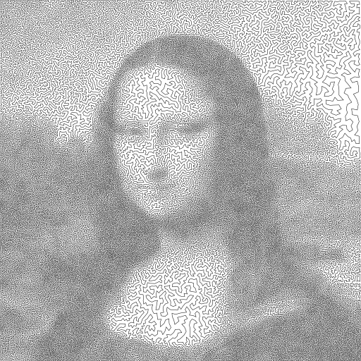
(a) mona-lisa100K

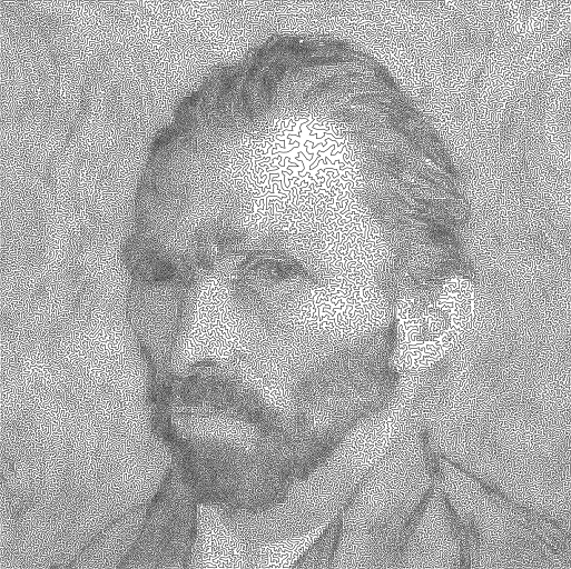
(b) vangogh120K

(c) venus140K

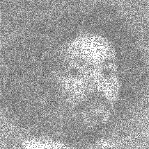
(d) pareja160K

(e) courbet180K

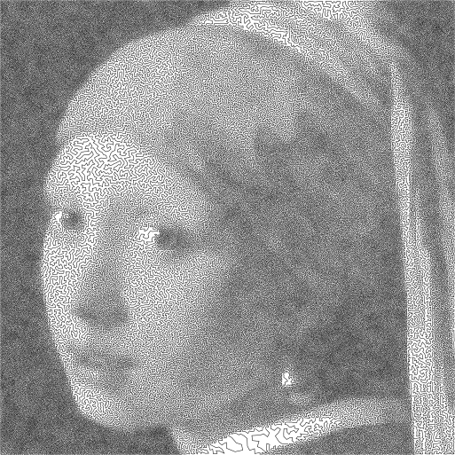
(f) earring200K

Figure 7: Visualisation of the best solutions obtained by the FACO for the TSP instances from TSP Art Instances [11].

It is worth noting that the proposed FACO combines a general-purpose metaheuristic (ACO) with a basic problem-specific LS (2-opt), which suggests that a more sophisticated, TSP-oriented approach should outperform it easily. Table 4 compares results of the FACO with the LKH solver by Helsgaun [22] which is the current state-of-the-art heuristic for solving the TSP [48, 42]. The results were obtained on the same machine (see 5.1 for the details). As expected, the LKH can find solutions of very high quality, i.e., differing at most 0.035% from the best-known results [11], within a few hours of computation time.

Table 4: Comparison with the state-of-the-art LKH TSP solver. The parameters of the LKH were set following [24].

Instance	LKH			FACO
	Tour length	Error [%]	Time [h]	Avg. tour length	Error [%]	Time [h]
mona-lisa100K	5758679	0.028	3.62	5793384	0.631	0.30
vangogh120K	6545491	0.029	5.10	6590084	0.710	0.39
venus140K	6812492	0.026	4.00	6861650	0.749	0.47
pareja160K	7622309	0.031	5.20	7681535	0.808	0.57
courbet180K	7891308	0.033	7.51	7958247	0.881	0.68
earring200K	8174554	0.035	7.94	8250696	0.967	0.86

Interestingly, a more general approach can be advantageous in some cases, making fewer assumptions about the problem. Recently, Hougardy and Zhong [25] have proposed a set of TSP instances explicitly designed to be hard to solve, especially for the exact TSP solvers like Concorde which is the fastest existing exact TSP solver [2]. Sizes of the instances range from several dozens to 100 000 nodes which are all points on a tetrahedron. For example, when solving an instance with 200 nodes, it was noted that Concorde was more than 1 000 000 times slower than for similar-sized TSP instances from the TSPLIB repository. Table 5 shows results obtained by the FACO for the hard-to-solve TSP instances with at least 500 nodes. The best-known results obtained with the LKH solver are also reported. As can be noticed, the FACO was able to find solutions of the same or even marginally better quality for a few of the largest instances, i.e., with at least 20 000 nodes.

Table 5: Results for the hard to solve TSP instances created by Hougardy and Zhong [25]. The best known results were obtained with the LKH solver [23]. The improved results are shown in bold.

Instance	Best known (LKH [23])	FACO
		Best	Worst	Mean	Time [s]
Tnm502	8 749 995	8 749 995	8 749 997	8 749 995.3	2.0
Tnm601	10 615 504	10 615 504	10 615 504	10 615 504.0	2.2
Tnm700	12 488 518	12 488 518	12 488 521	12 488 519.3	2.4
Tnm802	14 377 678	14 377 678	14 377 678	14 377 678.0	2.5
Tnm901	16 256 023	16 256 023	16 256 024	16 256 023.2	2.7
Tnm1000	18 137 296	18 137 298	18 137 298	18 137 298.0	2.9
Tnm2002	37 029 600	37 029 600	37 029 601	37 029 600.2	6.3
Tnm3001	55 939 349	55 939 349	55 939 352	55 939 349.5	10.1
Tnm4000	74 858 233	74 858 233	74 858 233	74 858 233.0	12.2
Tnm5002	93 784 081	93 784 081	93 784 081	93 784 081.0	17.3
Tnm6001	112 708 118	112 708 118	112 708 118	112 708 118.0	19.9
Tnm7000	131 633 371	131 633 371	131 633 374	131 633 372.0	26.1
Tnm8002	150 561 446	150 561 446	150 561 452	150 561 446.4	29.0
Tnm9001	169 487 546	169 487 546	169 487 548	169 487 546.1	31.9
Tnm10000	188 414 262	188 414 262	188 414 284	188 414 268.3	40.3
Tnm20002	377 692 238	377 692 219	377 692 257	377 692 235.5	100.6
Tnm30001	566 973 296	566 973 186	566 975 406	566 973 503.0	187.3
Tnm40000	756 254 243	756 254 121	756 257 737	756 254 389.0	291.3
Tnm50002	945 539 807	945 535 600	945 535 699	945 535 635.3	402.9
Tnm60001	1 134 820 740	1 134 816 445	1 134 816 532	1 134 816 474.6	546.6
Tnm70000	1 324 101 816	1 324 097 819	1 324 097 927	1 324 097 866.1	691.8
Tnm80002	1 513 392 208	1 513 381 620	1 513 391 253	1 513 383 905.6	797.4
Tnm90001	1 702 667 051	1 702 662 758	1 702 662 910	1 702 662 811.0	993.5
Tnm100000	1 891 945 975	1 891 945 653	1 891 945 678	1 891 945 662.5	1271.5

6 Conclusions

In this paper, we have shown that solving large-scale TSP instances efficiently with the ACO-based algorithm (MMAS) is possible with the help of a few relatively simple changes to the base algorithm and careful incorporation of a TSP-specific local search (2-opt). The main change concerns the constructive nature of the ACO, which involves building solutions to the problem from scratch in every iteration of the algorithm [17]. This approach contrasts perturbation-based heuristics, which apply several (typically small) modifications to the existing solutions, e.g., found in the previous iterations [21]. The latter approach is typically less time-consuming, particularly as the size of the problem increases. The proposed FACO follows a typical constructive behavior of the ACO but only until it selects a predefined number of solution components (edges) that are not present in the source solution. Next, the remaining portion of the solution is copied from the source solution. This strategy allows the FACO to gain the speed benefits of the perturbation-based approach without losing the constructive nature of the ACO. Moreover, keeping track of the differences between the constructed and the source solutions allows for a more efficient integration with the problem-specific LS (2-opt), which can focus only on the recently introduced components and skip the parts that did not change.

The proposed FACO demonstrates a robust performance when solving TSP instances with dozens to hundreds of thousands of nodes. For example, the algorithm required less than an hour to find solutions within 1% from the best-known results for the TSP Art Instances [11] with 100k to 200k nodes while running on a computer with an 8-core CPU. This can be seen as an improvement over the recently proposed ACO-based approaches, including the ACO-RPMM [35], the PartialACO [8], and the ACOTSP-MF [33]. As such, the FACO is a valuable addition to the family of ACO-based algorithms. Not surprisingly, the FACO cannot compete with the state-of-the-art LKH solver when solving the TSP instances from the TSPLIB or TSP Art datasets. However, due to making fewer assumptions about the problem, it is able to find the same or even slightly better solutions for the hard-to-solve TSP instances by Hougardy and Zhong [25].

Future work

The presented work may be extended in multiple directions. The proposed method of controlling the extent to which a new solution constructed by an ant differs from a selected previous (source) solution is largely problem-agnostic while being easy to implement at the same time. For these reasons, the method could prove valuable within contexts of different optimization problems. On the other hand, it should be possible to improve further the efficiency of the proposed FACO in the context of the TSP with the help of a more sophisticated LS, e.g., one considering also non-sequential moves [21]. Another direction points to a potential reduction of the FACO computation time with the help of the GPUs, or vector instructions (SIMD) offered by modern CPUs.

References

- Applegate [2011] David Applegate. The Traveling Salesman Problem : a Computational Study. Princeton University Press, Princeton, 2011. ISBN 978-0-691-12993-8.
- [2] David Applegate, Robert Bixby, Vasek Chvátal, and William Cook. Concorde. URL http://www.math.uwaterloo.ca/tsp/concorde/downloads/downloads.htm.
- Bell and McMullen [2004] John E. Bell and Patrick R. McMullen. Ant colony optimization techniques for the vehicle routing problem. Adv. Eng. Informatics, 18(1):41–48, 2004. doi: 10.1016/j.aei.2004.07.001. URL https://doi.org/10.1016/j.aei.2004.07.001.
- Bentley [1992] Jon Louis Bentley. Fast algorithms for geometric traveling salesman problems. INFORMS Journal on Computing, 4(4):387–411, 1992. doi: 10.1287/ijoc.4.4.387. URL https://doi.org/10.1287/ijoc.4.4.387.
- Bosch and Herman [2004] Robert Bosch and Adrianne Herman. Continuous line drawings via the traveling salesman problem. Oper. Res. Lett., 32(4):302–303, 2004. doi: 10.1016/j.orl.2003.10.001. URL https://doi.org/10.1016/j.orl.2003.10.001.
- Cecilia et al. [2013] José M. Cecilia, José M. García, Andy Nisbet, Martyn Amos, and Manuel Ujaldon. Enhancing data parallelism for ant colony optimization on gpus. J. Parallel Distrib. Comput., 73(1):42–51, 2013. doi: 10.1016/j.jpdc.2012.01.002. URL https://doi.org/10.1016/j.jpdc.2012.01.002.
- Cecilia et al. [2018] José M. Cecilia, Antonio Llanes, José L. Abellán, Juan Gómez-Luna, Li-Wen Chang, and Wen-Mei W. Hwu. High-throughput ant colony optimization on graphics processing units. J. Parallel Distrib. Comput., 113:261–274, 2018. doi: 10.1016/j.jpdc.2017.12.002. URL https://doi.org/10.1016/j.jpdc.2017.12.002.
- Chitty [2017] Darren M. Chitty. Applying ACO to large scale TSP instances. CoRR, abs/1709.03187, 2017. URL http://arxiv.org/abs/1709.03187.
- Choong et al. [2019] Shin Siang Choong, Li-Pei Wong, and Chee Peng Lim. An artificial bee colony algorithm with a modified choice function for the traveling salesman problem. Swarm and Evolutionary Computation, 44:622–635, 2019. doi: 10.1016/j.swevo.2018.08.004. URL https://doi.org/10.1016/j.swevo.2018.08.004.
- Colorni et al. [1991] Alberto Colorni, Marco Dorigo, Vittorio Maniezzo, et al. Distributed optimization by ant colonies. In Proceedings of the first European conference on artificial life, volume 142, pages 134–142. Paris, France, 1991.
- [11] William Cook. TSP Art Instances. URL https://www.math.uwaterloo.ca/tsp/data/art.
- Delévacq et al. [2013] Audrey Delévacq, Pierre Delisle, Marc Gravel, and Michaël Krajecki. Parallel ant colony optimization on graphics processing units. J. Parallel Distrib. Comput., 73(1):52–61, 2013. doi: 10.1016/j.jpdc.2012.01.003. URL https://doi.org/10.1016/j.jpdc.2012.01.003.
- Deng et al. [2019] Wu Deng, Junjie Xu, and Huimin Zhao. An improved ant colony optimization algorithm based on hybrid strategies for scheduling problem. IEEE Access, 7:20281–20292, 2019. doi: 10.1109/ACCESS.2019.2897580. URL https://doi.org/10.1109/ACCESS.2019.2897580.
- Dökeroglu et al. [2019] Tansel Dökeroglu, Ender Sevinç, Tayfun Kucukyilmaz, and Ahmet Cosar. A survey on new generation metaheuristic algorithms. Comput. Ind. Eng., 137, 2019. doi: 10.1016/j.cie.2019.106040. URL https://doi.org/10.1016/j.cie.2019.106040.
- Dorigo and Gambardella [1997] Marco Dorigo and Luca Maria Gambardella. Ant colony system: a cooperative learning approach to the traveling salesman problem. IEEE Trans. Evol. Comput., 1(1):53–66, 1997. doi: 10.1109/4235.585892. URL https://doi.org/10.1109/4235.585892.
- Dorigo and Stützle [2004] Marco Dorigo and Thomas Stützle. Ant colony optimization. MIT Press, 2004. ISBN 978-0-262-04219-2. doi: 10.7551/mitpress/1290.001.0001. URL https://doi.org/10.7551/mitpress/1290.001.0001.
- Dorigo et al. [1996] Marco Dorigo, Vittorio Maniezzo, and Alberto Colorni. Ant system: optimization by a colony of cooperating agents. IEEE Trans. Systems, Man, and Cybernetics, Part B, 26(1):29–41, 1996. doi: 10.1109/3477.484436. URL https://doi.org/10.1109/3477.484436.
- Engelbrecht [2005] Andries Petrus Engelbrecht. Fundamentals of Computational Swarm Intelligence. Wiley, 2005. ISBN 978-0-470-09191-3. URL http://eu.wiley.com/WileyCDA/WileyTitle/productCd-0470091916.html.
- Gambardella et al. [2012] L.M. Gambardella, R. Montemanni, and D. Weyland. Coupling ant colony systems with strong local searches. European Journal of Operational Research, 220(3):831–843, 2012. ISSN 0377-2217. doi: https://doi.org/10.1016/j.ejor.2012.02.038. URL https://www.sciencedirect.com/science/article/pii/S0377221712001889.
- Guntsch and Middendorf [2002] Michael Guntsch and Martin Middendorf. A population based approach for ACO. In Stefano Cagnoni, Jens Gottlieb, Emma Hart, Martin Middendorf, and Günther R. Raidl, editors, Applications of Evolutionary Computing, EvoWorkshops 2002: EvoCOP, EvoIASP, EvoSTIM/EvoPLAN, Kinsale, Ireland, April 3-4, 2002, Proceedings, volume 2279 of Lecture Notes in Computer Science, pages 72–81. Springer, 2002. doi: 10.1007/3-540-46004-7_8. URL https://doi.org/10.1007/3-540-46004-7_8.
- Helsgaun [2000] Keld Helsgaun. An effective implementation of the lin-kernighan traveling salesman heuristic. Eur. J. Oper. Res., 126(1):106–130, 2000. doi: 10.1016/S0377-2217(99)00284-2. URL https://doi.org/10.1016/S0377-2217(99)00284-2.
- Helsgaun [2009] Keld Helsgaun. General k-opt submoves for the lin-kernighan TSP heuristic. Math. Program. Comput., 1(2-3):119–163, 2009. doi: 10.1007/s12532-009-0004-6. URL https://doi.org/10.1007/s12532-009-0004-6.
- Helsgaun [2018a] Keld Helsgaun. Best LKH Solutions for Tnm Instances, 2018a. URL http://webhotel4.ruc.dk/~keld/research/LKH/BestLKHsolutionsforTnminstances.pdf.
- Helsgaun [2018b] Keld Helsgaun. Using POPMUSIC for candidate set generation in the lin-kernighan-helsgaun TSP solver. Technical report, Department of Computer Science, Roskilde University, DK-4000 Roskilde, Denmark, July 2018b. URL http://webhotel4.ruc.dk/~keld/research/LKH/POPMUSIC˙REPORT.pdf.
- Hougardy and Zhong [2021] Stefan Hougardy and Xianghui Zhong. Hard to solve instances of the euclidean traveling salesman problem. Math. Program. Comput., 13(1):51–74, 2021. doi: 10.1007/s12532-020-00184-5. URL https://doi.org/10.1007/s12532-020-00184-5.
- Ismkhan [2017] Hassan Ismkhan. Effective heuristics for ant colony optimization to handle large-scale problems. Swarm and Evolutionary Computation, 32:140–149, 2017. doi: 10.1016/j.swevo.2016.06.006. URL https://doi.org/10.1016/j.swevo.2016.06.006.
- Kennedy [2006] James Kennedy. Swarm intelligence. In Albert Y. Zomaya, editor, Handbook of Nature-Inspired and Innovative Computing - Integrating Classical Models with Emerging Technologies, pages 187–219. Springer, 2006. doi: 10.1007/0-387-27705-6_6. URL https://doi.org/10.1007/0-387-27705-6_6.
- Leguizamon and Michalewicz [1999] Guillermo Leguizamon and Zbigniew Michalewicz. A new version of ant system for subset problems. In Proceedings of the 1999 Congress on Evolutionary Computation-CEC99 (Cat. No. 99TH8406), volume 2, pages 1459–1464. IEEE, 1999.
- Lin [1965] Shen Lin. Computer solutions of the traveling salesman problem. Bell System Technical Journal, 44(10):2245–2269, 1965.
- Lin and Kernighan [1973] Shen Lin and Brian W. Kernighan. An effective heuristic algorithm for the traveling-salesman problem. Oper. Res., 21(2):498–516, 1973. doi: 10.1287/opre.21.2.498. URL https://doi.org/10.1287/opre.21.2.498.
- López-Ibáñez and Blum [2010] Manuel López-Ibáñez and Christian Blum. Beam-aco for the travelling salesman problem with time windows. Comput. Oper. Res., 37(9):1570–1583, 2010. doi: 10.1016/j.cor.2009.11.015. URL https://doi.org/10.1016/j.cor.2009.11.015.
- Marinakis et al. [2011] Yannis Marinakis, Magdalene Marinaki, and Georgios Dounias. Honey bees mating optimization algorithm for the euclidean traveling salesman problem. Inf. Sci., 181(20):4684–4698, 2011. doi: 10.1016/j.ins.2010.06.032. URL https://doi.org/10.1016/j.ins.2010.06.032.
- Martínez and García [2021] Pablo Antonio Martínez and José M. García. ACOTSP-MF: A memory-friendly and highly scalable ACOTSP approach. Eng. Appl. Artif. Intell., 99:104131, 2021. doi: 10.1016/j.engappai.2020.104131. URL https://doi.org/10.1016/j.engappai.2020.104131.
- Nezamabadi-pour et al. [2006] Hossein Nezamabadi-pour, Saeid Saryazdi, and Esmat Rashedi. Edge detection using ant algorithms. Soft Comput., 10(7):623–628, 2006. doi: 10.1007/s00500-005-0511-y. URL https://doi.org/10.1007/s00500-005-0511-y.
- Peake et al. [2019] Joshua Peake, Martyn Amos, Paraskevas Yiapanis, and Huw Lloyd. Scaling techniques for parallel ant colony optimization on large problem instances. In Anne Auger and Thomas Stützle, editors, Proceedings of the Genetic and Evolutionary Computation Conference, GECCO 2019, Prague, Czech Republic, July 13-17, 2019, pages 47–54. ACM, 2019. doi: 10.1145/3321707.3321832. URL https://doi.org/10.1145/3321707.3321832.
- Pedemonte et al. [2011] Martín Pedemonte, Sergio Nesmachnow, and Héctor Cancela. A survey on parallel ant colony optimization. Appl. Soft Comput., 11(8):5181–5197, 2011. doi: 10.1016/j.asoc.2011.05.042. URL https://doi.org/10.1016/j.asoc.2011.05.042.
- Shmygelska and Hoos [2005] Alena Shmygelska and Holger H. Hoos. An ant colony optimisation algorithm for the 2d and 3d hydrophobic polar protein folding problem. BMC Bioinform., 6:30, 2005. doi: 10.1186/1471-2105-6-30. URL https://doi.org/10.1186/1471-2105-6-30.
- Skinderowicz [2013] Rafał Skinderowicz. Ant colony system with selective pheromone memory for SOP. In Costin Badica, Ngoc Thanh Nguyen, and Marius Brezovan, editors, Computational Collective Intelligence. Technologies and Applications - 5th International Conference, ICCCI 2013, Craiova, Romania, September 11-13, 2013, Proceedings, volume 8083 of Lecture Notes in Computer Science, pages 711–720. Springer, 2013. doi: 10.1007/978-3-642-40495-5_71. URL https://doi.org/10.1007/978-3-642-40495-5_71.
- Skinderowicz [2016] Rafał Skinderowicz. The GPU-based parallel Ant Colony System. J. Parallel Distrib. Comput., 98:48–60, 2016. doi: 10.1016/j.jpdc.2016.04.014. URL https://doi.org/10.1016/j.jpdc.2016.04.014.
- Skinderowicz [2020] Rafał Skinderowicz. Implementing a GPU-based parallel MAX-MIN ant system. Future Gener. Comput. Syst., 106:277–295, 2020. doi: 10.1016/j.future.2020.01.011. URL https://doi.org/10.1016/j.future.2020.01.011.
- Stützle and Hoos [2000] Thomas Stützle and Holger H. Hoos. MAX-MIN ant system. Future Generation Comp. Syst., 16(8):889–914, 2000. doi: 10.1016/S0167-739X(00)00043-1. URL https://doi.org/10.1016/S0167-739X(00)00043-1.
- Taillard [2021] Éric D Taillard. A linearithmic heuristic for the travelling salesman problem. European Journal of Operational Research, 2021.
- Taillard and Helsgaun [2019] Éric D. Taillard and Keld Helsgaun. POPMUSIC for the travelling salesman problem. Eur. J. Oper. Res., 272(2):420–429, 2019. doi: 10.1016/j.ejor.2018.06.039. URL https://doi.org/10.1016/j.ejor.2018.06.039.
- Tirado et al. [2017] Felipe Tirado, Ricardo J. Barrientos, Paulo González, and Marco Mora. Efficient exploitation of the xeon phi architecture for the ant colony optimization (ACO) metaheuristic. J. Supercomput., 73(11):5053–5070, 2017. doi: 10.1007/s11227-017-2124-5. URL https://doi.org/10.1007/s11227-017-2124-5.
- Yang et al. [2016] Xin-She Yang, Suash Deb, Simon Fong, Xingshi He, and Yuxin Zhao. From swarm intelligence to metaheuristics: Nature-inspired optimization algorithms. Computer, 49(9):52–59, 2016. doi: 10.1109/MC.2016.292. URL https://doi.org/10.1109/MC.2016.292.
- Zhong et al. [2019] Yiwen Zhong, Lijin Wang, Min Lin, and Hui Zhang. Discrete pigeon-inspired optimization algorithm with metropolis acceptance criterion for large-scale traveling salesman problem. Swarm Evol. Comput., 48:134–144, 2019. doi: 10.1016/j.swevo.2019.04.002. URL https://doi.org/10.1016/j.swevo.2019.04.002.
- Zhou et al. [2018] Yi Zhou, Fazhi He, Neng Hou, and Yimin Qiu. Parallel ant colony optimization on multi-core SIMD cpus. Future Generation Comp. Syst., 79:473–487, 2018. doi: 10.1016/j.future.2017.09.073. URL https://doi.org/10.1016/j.future.2017.09.073.
- Éric D. Taillard and Helsgaun [2019] Éric D. Taillard and Keld Helsgaun. POPMUSIC for the travelling salesman problem. European Journal of Operational Research, 272(2):420–429, 2019. ISSN 0377-2217. doi: https://doi.org/10.1016/j.ejor.2018.06.039. URL https://www.sciencedirect.com/science/article/pii/S0377221718305745.