Gamma-Shadowed Two-Ray with Diffuse Power Composite Fading Model

Abstract

In this paper, a novel gamma-shadowed two-ray with diffuse power (GS-TWDP) composite fading model is proposed. The model is intended for modeling propagation in the emerging wireless networks working at millimeter wave (mmWave) frequencies, and is obtained as a combination of TWDP distribution for description of multipath effects and gamma distribution for modeling variations due to shadowing. After derivation of the exact probability density function (PDF), cumulative distribution function (CDF) and moment generating functions (MGF) expressions are obtained. Proposed model is verified by comparing the analytically obtained results with those measured at 28 GHz and reported in literature. Two upper bound average symbol error probability (ASEP) expressions are then derived for M-ary rectangular quadrature amplitude modulation (RQAM) by employing Chernoff and Chiani approximations of Gaussian Q-function, and are used to investigate relationship between GS-TWDP parameters and system performance. All the results are verified by Monte-Carlo simulation.

I Introduction

Over the last decade, mmWave bands have attracted large research interest as candidate bands for implementation of the future mobile networks. However, signals propagating in these bands exhibit different characteristics than those propagating at frequencies below 6 GHz. For example, it is empirically shown that at such high frequencies, multipath-caused fast variations of the received signal about its local mean can oftentimes be worse than those in Rayleigh channels [1, 2], which is phenomena not notably observed at lower frequencies. Consequently, TWDP is proposed as a substitute to traditional Rayleigh or Rician fading models, for modeling multipath effect on signal propagating within the mmWave bands.

Thereat, Rayleigh and Rician fading models assume that the received signal is composed of many weak diffuse components and none or just one strong specular component, respectively. As such, these models can not be used for modeling worse-than-Rayleigh fading conditions. On the contrary, TWDP assumes that the received signal is composed of two strong specular in addition to diffuse components, which makes the model applicable for modeling not just worse-than-Rayleigh, but also Rayleigh and better-than-Rayleigh fading conditions [3]. Therewithal, it is shown that TWDP provides better fit than traditional models to empirical data collected at mmWave frequencies, even when multipath-caused variations are less severe than those observed in Rayleigh channel. The aforementioned is confirmed by ray-tracing simulation when modeling vehicular-to-infrastructure (V2I) communication scenario [4], and by measurements, when modeling vehicle-to-vehicle (V2V) communication in urban environment at 60 GHz [5]. Two indoor mmWave measurement campaigns performed in [6] revealed that TWDP model is more adequate than traditional models for characterization of indoor mmWave communication, and that it is also the best choice for modeling near-body mmWave channels, both in the front and in the back region [2].

Obviously, TWDP model is highly applicable for description of fast amplitude variations in mmWave bands in varieties of propagation scenarios. However, it takes into account only multipath-caused variations of the received signal about the local mean and as such, it assumes that the local mean value is constant. Nevertheless, due to shadowing effect, which manifests when the receiver or objects in the environment notably move, local mean value starts to vary too. Consequently, when estimating overall system performance metrics (such as error rate probability, outage probability, and so on) in mmWave band, slow variations of the signal’s local mean value also should be considered. Accordingly, composite fading models - which takes into consideration both, fast multipath-caused variations of a signal about the local mean and slow shadowing-caused variation of the local mean - are the only appropriate models for characterization of propagation in the dynamic environments. In these circumstances, it is necessary to identify shadowing model which could be used in conjunction with TWDP for appropriate description of propagation at mmWave frequencies.

Thereat, in the majority of literature, shadowing-caused variations are assumed to be lognormally distributed [8, 9], since lognormal distribution the most accurately describes corresponding measurement results, both in traditional [10, 11], as well as in mmWave bands [12, 13]. However, mathematical form of lognormal PDF is not convenient for analytic manipulations, since it hinders calculation of closed-form expressions for most performance metrics of interest [9]. As a solution, computationally more suitable distributions (such as gamma, inverse-gamma, inverse-Gaussian etc.) have been proposed as a substitute for lognormal PDF. Among them, gamma is the most frequently employed, since it has computationally convenient form and provides similar fit to empirical data as lognormal PDF in many communication scenarios [9, 14]. So, to date, for varieties of multipath distributions, composite fading models such as Rayleigh-Gamma [15], Rice-Gamma [16], Nakagami-Gamma [8], $\kappa\mu$-Gamma [17] etc., are proposed by employing gamma PDF for modeling shadowing effect.

Also, for TWDP distributed multipath, the effect of gamma shadowing on overall system performances is considered within the fluctuating two-ray (FTR) model proposed in [18]. However, the model assumes that shadowing affects only two specular components, while the mean power of diffuse components remains unaffected, which makes FTR inapplicable for modeling propagation scenarios in which all components within the local mean fluctuate.

However, when scatterers are in the vicinity of transceivers, beside the specular components, diffuse components will also travel alongside most of the way [7]. Consequently, the eventual channel fluctuations would affect all of them simultaneously [7]. So, in the described scenario, as the users or the surrounding objects move, human body or any other type of shadowing will affect not only specular but also diffuse components. Since, in addition, diffuse components in mmWave band can account for up to 40% of the total received power [19, 20], there is a clear motivation to investigate the effect of gamma-distributed shadowing which simultaneously affects both, diffuse and specular components, on overall performance of systems operating in mmWave bands.

Considering the aforesaid, in this paper, a novel composite fading model called gamma-shadowed TWDP (GS-TWDP) is proposed by assuming TWDP distributed signal with its local mean distributed following gamma PDF. For the proposed model, the appropriate chief probability functions are derived as simple closed-form expressions and their applicability for derivation of performance metrics is demonstrated by deriving the upper ASEP bounds for M-ary RQAM modulated signal, obtained using Chernoff and Chiani approximations of a Gaussian Q-function. Proposed model is also empirically verified by measurements performed at 28 GHz in [21], confirming its applicability for modeling overall signal variations at mmWave frequencies.

The rest of the paper is organized as follows: In Section II, GS-TWDP fading model is introduced, followed by derivation of its chief probability functions, i.e. PDF, CDF and MGF. Verification of the proposed model is performed is Section III. In Section IV, approximate M-ary RQAM ASEPs of a signal propagating in GS-TWDP fading channel are deduced, while the impact of different model’s parameters on ASEP are investigated in Section V. Conclusions are provided in Section VI.

II Statistical characterization of Gamma-shadowed TWDP fading model

II-A TWDP multipath fading model

TWDP is multipath fading model introduced by Durgin et al. [3] for modeling Rayleigh, better-than-Rayleigh and worse-than-Rayleigh fading conditions. It assumes that the received complex envelope $r(t)$ is composed of two strong specular components $v_{1}(t)$ and $v_{2}(t)$ and many low power diffuse components:

$$\begin{split}r(t)&=v_{1}(t)+v_{2}(t)+n(t)\\ &=V_{1}\exp{\left(j\Phi_{1}\right)}+V_{2}\exp{\left(j\Phi_{2}\right)}+n(t)\end{split}$$ (1)

Within the model, specular components are assumed to be mutually independent with constant magnitudes $V_{1}$ and $V_{2}$ and phases $\Phi_{1}$ and $\Phi_{2}$ uniformly distributed in $[0,2\pi)$, respectively, while diffuse components are treated as a complex zero-mean Gaussian random process $n(t)$ with the average power $2\sigma^{2}$. Considering the aforesaid, in a frequency-flat, slowly varying TWDP fading channel, the received envelope has the following PDF (which is obtained after the random variable transformation of the equation [22, eq. (6)]):

$$\begin{split}p{{}_{r}}(x)&=e^{-K}\sum_{j=0}^{\infty}\frac{2K^{j}t_{j}}{(j!)^{2}}\left(\frac{K+1}{\Omega}\right)^{j+1}\\ &\times x^{2j+1}\exp{\left(-\frac{x^{2}(K+1)}{\Omega}\right)},\leavevmode\nobreak\ x>0\end{split}$$ (2)

where $t_{j}$ is defined as:

$$t_{j}=\sum_{k=0}^{j}\left(\frac{\Gamma}{\Gamma^{2}+1}\right)^{k}\binom{j}{k}\sum_{l=0}^{k}\binom{k}{l}I_{2l-k}\left(-\frac{2\Gamma K}{1+\Gamma^{2}}\right)$$ (3)

or [22, eq. (14)]:

$$t_{j}=\frac{1}{2\pi}\int_{0}^{2\pi}\exp{\left(-\frac{2\Gamma K\cos{\alpha}}{1+\Gamma^{2}}\right)}\left(1+\frac{2\Gamma}{1+\Gamma^{2}}\cos{\alpha}\right)^{j}\mathop{}\!\mathrm{d}{\alpha}$$ (4)

if expressed in integral form. Thereat, in (2) - (4), $I_{\nu}(\cdot)$ is modified Bessel function of a first kind and order $\nu$, $K$ reflects the ratio between powers of specular and diffuse components and is defined as $K=(V_{1}^{2}+V_{2}^{2})/2\sigma^{2}$ and $\Gamma=V_{2}/V_{1}$ is the ratio between magnitudes of two specular components. In such conditions, the average power of $r(t)$ given by (1), i.e. its local mean, is equal to $\Omega=V_{1}^{2}+V_{2}^{2}+2\sigma^{2}$, and due to initial assumption on $V_{1}$ and $V_{2}$ constancy, it is obviously assumed to be constant over the multipath effect’s observation interval. 

II-B Gamma shadowing model

However, when the transceiver and/or the surrounding objects significantly move, due to shadowing effect, the local mean $\Omega$ starts to varies about the constant area mean power $P_{r}$ too. These variations have been traditionally modeled as a lognormal random variable, with its PDF given as:

$$\begin{split}p_{\Omega}(x)=\frac{1}{x\sqrt{2\pi\sigma_{s}^{2}}}\exp{\left(-\frac{\ln^{2}{\left(x/P_{r}\right)}}{2\sigma_{s}^{2}}\right)},\leavevmode\nobreak\ \leavevmode\nobreak\ \leavevmode\nobreak\ \leavevmode\nobreak\ x>0\end{split}$$ (5)

where $\sigma_{s}$ is shadowing standard deviation, whose values are usually reported in literature for different propagation conditions. However, analytical form of lognormal distribution is not appropriate for mathematical manipulations and can not be used for calculation of closed-form expressions for error probabilities of differently modulated signals propagating in lognormally distributed shadowing channels.

Accordingly, for many years, gamma distribution has been used as a substitute PDF, given as:

$$\begin{split}p_{\Omega}(x)=\frac{1}{{\mathchoice{\raisebox{0.0pt}{\scalebox{1.0}[-1.0]{$\displaystyle\mathbb{L}$}}}{\raisebox{0.0pt}{\scalebox{1.0}[-1.0]{$\textstyle\mathbb{L}$}}}{\raisebox{0.0pt}{\scalebox{1.0}[-1.0]{$\scriptstyle\mathbb{L}$}}}{\raisebox{0.0pt}{\scalebox{1.0}[-1.0]{$\scriptscriptstyle\mathbb{L}$}}}}[m]}\left(\frac{m}{\Omega_{s}}\right)^{m}x^{m-1}\exp{\left(-x\frac{m}{\Omega_{s}}\right)},x>0\end{split}$$ (6)

where ${\mathchoice{\raisebox{0.0pt}{\scalebox{1.0}[-1.0]{$\displaystyle\mathbb{L}$}}}{\raisebox{0.0pt}{\scalebox{1.0}[-1.0]{$\textstyle\mathbb{L}$}}}{\raisebox{0.0pt}{\scalebox{1.0}[-1.0]{$\scriptstyle\mathbb{L}$}}}{\raisebox{0.0pt}{\scalebox{1.0}[-1.0]{$\scriptscriptstyle\mathbb{L}$}}}}[\cdot]$ is a gamma function, while $\Omega_{s}$ and $m$ represent gamma shadowing mean power in the area of interest and shadowing severity, respectively. If these parameters are chosen by matching means and variances of the lognormal and gamma PDFs, they can be expressed in terms of $\sigma_{s}$ and $P_{r}$ as [8]:

$$m=\frac{1}{\exp{\left(\sigma_{s}^{2}\right)}-1}\leavevmode\nobreak\ \leavevmode\nobreak\ \leavevmode\nobreak\ \leavevmode\nobreak\ \Omega_{s}=P_{r}\sqrt{\frac{m+1}{m}}$$ (7)

For such obtained parameters, it is shown that gamma PDF closely approximate lognormal distribution, especially in upper tail region of the PDF [8]. However, its analytical form is more favorable for mathematical manipulation than the form of a lognormal PDF, which all make gamma distribution the promising candidate for modeling shadowing-caused variations in conjunction with TWDP multipath fading.

II-C GS-TWDP composite fading model

Under the above assumptions, PDF of the GS-TWDP envelope $r_{c}$ can be determined by averaging the conditional TWDP PDF with respect to $\Omega$:

$$\begin{split}p_{r_{c}}(x)=\int_{0}^{\infty}p_{r}(x|\omega)p_{\Omega}(\omega)\mathop{}\!\mathrm{d}{\omega}\end{split}$$ (8)

which can be solved using [25, eq. (2.3.16 (1))] as:

$$\begin{split}p{{}_{r_{c}}}(x)&=\frac{4e^{-K}}{{\mathchoice{\raisebox{0.0pt}{\scalebox{1.0}[-1.0]{$\displaystyle\mathbb{L}$}}}{\raisebox{0.0pt}{\scalebox{1.0}[-1.0]{$\textstyle\mathbb{L}$}}}{\raisebox{0.0pt}{\scalebox{1.0}[-1.0]{$\scriptstyle\mathbb{L}$}}}{\raisebox{0.0pt}{\scalebox{1.0}[-1.0]{$\scriptscriptstyle\mathbb{L}$}}}}[m]}\sum_{j=0}^{\infty}\frac{K^{j}t_{j}}{(j!)^{2}}\left((K+1)\frac{m}{\Omega_{s}}\right)^{\frac{m+j+1}{2}}\\ &\times{\mathbb{K}}_{1+j-m}\left[2x\sqrt{(K+1)\frac{m}{\Omega_{s}}}\right]x^{m+j}\end{split}$$ (9)

where ${\mathbb{K}}_{\nu}(\cdot)$ represents modified Bessel function of the second kind and order $\nu$.

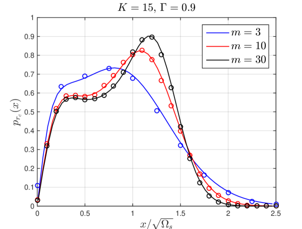
(a)

(b)

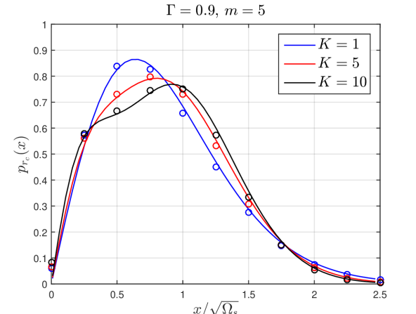
(c)

Figure 1: Analytical (solid line) and Monte-Carlo simulated (dots) GS-TWDP normalized envelope PDF for different values of: (a) $m$ ($K=15$, $\Gamma=0.9$) (b) $\Gamma$ ($K=15$, $m=5$) (c) $K$ ($\Gamma=0.9$, $m=5$)

Considering the aforesaid, the behaviour of GS-TWDP PDF can be observed from Fig. 1, which depicts PDFs expressed by (9) for different arbitrary values of parameters $K$, $\Gamma$ and $m$ (obtained with maximum 100 summation terms), together with the corresponding simulated PDFs generated by using Monte-Carlo samples which clearly validate derived analytical PDF expression.

Fig. 1 also shows that proposed GS-TWDP distribution exhibits bimodal behavior, which is observed within the empirical PDF obtained by measurements on 28 GHz in [21]. Accordingly, based on [18], it can be served for recreation of the wide heterogeneity of random fluctuations that affect the mmWave radio signal when propagating in the presence of multiple scatterers.

From Fig. 1 also can be observed that bimodality becomes more pronounced with the increment of $K$, $\Gamma$ or $m$, in cases when two other parameters remain unchanged, and that it reaches its maximum when simultaneously $\Gamma\to 1$ and $K$ is large (which is the combination of corresponding parameters that represents conditions in worse-than-Rayleigh fading channels).

In addition to the aforesaid, using the identity [26, eq. 6.561.16], one can prove that $\int_{0}^{\infty}p_{r_{c}}(x)\mathop{}\!\mathrm{d}{x}=1$. It is also interesting to note that derived GS-TWDP envelope PDF expression for $\Gamma=0$ reduces to a Gamma-shadowed Rician PDF given in [16], while for $K=0$, GS-TWDP becomes Gamma-shadowed Rayleigh PDF. It also can be shown that in no-shadowing case obtained as $m\to\infty$, PDF (9) reduces to TWDP PDF given in [22].

Finally, it is noteworthy to observe that GS-TWDP and FTR [7] models are identical only when $m\to\infty$ (which is no shadowing case) and $K\to\infty$ (which is no multipath case), while in all other cases, models will provide different results.

II-C1 Moments

Derived PDF can be used to obtain $n$-th order moments of the GS-TWDP envelope, by using the expression:

$$\begin{split}\mathbb{E}\{r_{c}^{n}\}&=\int_{0}^{\infty}x^{n}p_{r_{c}}(x)\mathop{}\!\mathrm{d}{x}\\ &=\frac{4e^{-K}}{{\mathchoice{\raisebox{0.0pt}{\scalebox{1.0}[-1.0]{$\displaystyle\mathbb{L}$}}}{\raisebox{0.0pt}{\scalebox{1.0}[-1.0]{$\textstyle\mathbb{L}$}}}{\raisebox{0.0pt}{\scalebox{1.0}[-1.0]{$\scriptstyle\mathbb{L}$}}}{\raisebox{0.0pt}{\scalebox{1.0}[-1.0]{$\scriptscriptstyle\mathbb{L}$}}}}[m]}\sum_{j=0}^{\infty}\frac{K^{j}t_{j}}{(j!)^{2}}\left((K+1)\frac{m}{\Omega_{s}}\right)^{\frac{m+j+1}{2}}\\ &\times\int_{0}^{\infty}\mathbb{K}_{1+j-m}\left[2x\sqrt{(K+1)\frac{m}{\Omega_{s}}}\right]x^{m+j+n}\mathop{}\!\mathrm{d}{x}\end{split}$$ (10)

which can be solved with the help of [27, 2.16.2(2)] and written in the following form:

$$\begin{split}\mathbb{E}\{r_{c}^{n}\}&=\frac{e^{-K}}{{\mathchoice{\raisebox{0.0pt}{\scalebox{1.0}[-1.0]{$\displaystyle\mathbb{L}$}}}{\raisebox{0.0pt}{\scalebox{1.0}[-1.0]{$\textstyle\mathbb{L}$}}}{\raisebox{0.0pt}{\scalebox{1.0}[-1.0]{$\scriptstyle\mathbb{L}$}}}{\raisebox{0.0pt}{\scalebox{1.0}[-1.0]{$\scriptscriptstyle\mathbb{L}$}}}}[m_{s}]}\sum_{j=0}^{\infty}\frac{K^{j}t_{j}}{(j!)^{2}}\left((K+1)\frac{m_{s}}{\Omega_{s}}\right)^{-\frac{n}{2}}\\ &\times{\mathchoice{\raisebox{0.0pt}{\scalebox{1.0}[-1.0]{$\displaystyle\mathbb{L}$}}}{\raisebox{0.0pt}{\scalebox{1.0}[-1.0]{$\textstyle\mathbb{L}$}}}{\raisebox{0.0pt}{\scalebox{1.0}[-1.0]{$\scriptstyle\mathbb{L}$}}}{\raisebox{0.0pt}{\scalebox{1.0}[-1.0]{$\scriptscriptstyle\mathbb{L}$}}}}\left[1+j+\frac{n}{2}\right]{\mathchoice{\raisebox{0.0pt}{\scalebox{1.0}[-1.0]{$\displaystyle\mathbb{L}$}}}{\raisebox{0.0pt}{\scalebox{1.0}[-1.0]{$\textstyle\mathbb{L}$}}}{\raisebox{0.0pt}{\scalebox{1.0}[-1.0]{$\scriptstyle\mathbb{L}$}}}{\raisebox{0.0pt}{\scalebox{1.0}[-1.0]{$\scriptscriptstyle\mathbb{L}$}}}}\left[m_{s}+\frac{n}{2}\right]\end{split}$$ (11)

where $\mathbb{E}\{\cdot\}$ is the expectation operator. Using (11), it also can be shown that the second moment of the envelope $\mathbb{E}\{r_{c}^{2}\}$ is equal to $\Omega_{s}$. Namely, according to (11), second moment can be written as:

$$\mathbb{E}\{r_{c}^{2}\}=\frac{e^{-K}}{K+1}\sum_{j=0}^{\infty}\frac{K^{j}t_{j}(j+1)}{(j!)}{\Omega_{s}}$$ (12)

where $t_{j}$ is given by (4). After changing the order of integration and summation, the last expression becomes equal to:

$$\mathbb{E}\{r_{c}^{2}\}=\frac{\Omega_{s}}{K+1}\int_{0}^{2\pi}e^{-a}\sum_{j=0}^{\infty}\frac{a^{j}(j+1)}{(j!)}\mathop{}\!\mathrm{d}{\alpha}$$ (13)

where $a=K\left(1+2\Gamma/(1+\Gamma^{2})\right)\cos{\alpha}$. Accordingly, with the help of [25, 5.2.9(1)], it can be easily shown that the summation term in (13) is equal to $e^{a}(1+K)$, which makes $\mathbb{E}\{r_{c}^{2}\}=\Omega_{s}$.

II-C2 PDF, CDF and MGF

Based on (9) and the above conclusion, it is now possible to obtaine closed-form expressions for GS-TWDP PDF of the SNR, as well as its closed-form CDF and MGF expressions.

So, considering the fact that the ratio between instantaneous SNR $\gamma$, and average SNR $\gamma_{0}$ can be expressed as:

$$\frac{\gamma}{\gamma_{0}}=\frac{r_{c}^{2}}{\mathbb{E}\{r_{c}^{2}\}}=\frac{r_{c}^{2}}{\Omega_{s}}$$ (14)

PDF of the SNR in GS-TWDP fading channel can be obtained from (8) by simple random variable transformation, as follows:

$$\begin{split}p_{\gamma}(\gamma)&=\frac{2e^{-K}}{{\mathchoice{\raisebox{0.0pt}{\scalebox{1.0}[-1.0]{$\displaystyle\mathbb{L}$}}}{\raisebox{0.0pt}{\scalebox{1.0}[-1.0]{$\textstyle\mathbb{L}$}}}{\raisebox{0.0pt}{\scalebox{1.0}[-1.0]{$\scriptstyle\mathbb{L}$}}}{\raisebox{0.0pt}{\scalebox{1.0}[-1.0]{$\scriptscriptstyle\mathbb{L}$}}}}[m]}\sum_{j=0}^{\infty}\frac{K^{j}t_{j}}{(j!)^{2}}\left((K+1)\frac{m}{\gamma_{0}}\right)^{\frac{m+j+1}{2}}\\ &\times{\mathbb{K}}_{1+j-m}\left[2\sqrt{\gamma(K+1)\frac{m}{\gamma_{0}}}\right]\gamma^{\frac{m+j-1}{2}}\end{split}$$ (15)

On the other side, CDF of the SNR can be derived by integrating (15), using the expression $F_{\gamma}(\gamma)=\int_{0}^{\gamma}p_{\gamma}(x)\mathop{}\!\mathrm{d}{x}$:

$$\begin{split}F_{\gamma}(\gamma)&=\frac{2e^{-K}}{{\mathchoice{\raisebox{0.0pt}{\scalebox{1.0}[-1.0]{$\displaystyle\mathbb{L}$}}}{\raisebox{0.0pt}{\scalebox{1.0}[-1.0]{$\textstyle\mathbb{L}$}}}{\raisebox{0.0pt}{\scalebox{1.0}[-1.0]{$\scriptstyle\mathbb{L}$}}}{\raisebox{0.0pt}{\scalebox{1.0}[-1.0]{$\scriptscriptstyle\mathbb{L}$}}}}[m]}\sum_{j=0}^{\infty}\frac{K^{j}t_{j}}{(j!)^{2}}\left((K+1)\frac{m}{\gamma_{0}}\right)^{\frac{m+j+1}{2}}\\ &\times\int_{0}^{\gamma}{\mathbb{K}}_{1+j-m}\left(2\sqrt{x(K+1)\frac{m}{\gamma_{0}}}\right)x^{\frac{m+j-1}{2}}\mathop{}\!\mathrm{d}{x}\end{split}$$ (16)

which can be solved with the help of [27, 2.16.3(2)], as:

$$\begin{split}F_{\gamma}(\gamma)&=\frac{e^{-K}}{\Gamma{[m]}}\sum_{j=0}^{\infty}\frac{K^{j}t_{j}}{(j!)^{2}}\left(\frac{1}{1+j}\left(\frac{(K+1)m}{\gamma_{0}}\gamma\right)^{1+j}\right.\\ &\left.\times_{1}F_{2}\left[1+j;2+j,2+j-m;\frac{(K+1)m}{\gamma_{0}}\gamma\right]\right.\\ &\left.\times{\mathchoice{\raisebox{0.0pt}{\scalebox{1.0}[-1.0]{$\displaystyle\mathbb{L}$}}}{\raisebox{0.0pt}{\scalebox{1.0}[-1.0]{$\textstyle\mathbb{L}$}}}{\raisebox{0.0pt}{\scalebox{1.0}[-1.0]{$\scriptstyle\mathbb{L}$}}}{\raisebox{0.0pt}{\scalebox{1.0}[-1.0]{$\scriptscriptstyle\mathbb{L}$}}}}[m-j-1]+\frac{1}{m}\left(\frac{(K+1)m}{\gamma_{0}}\gamma\right)^{m}{\mathchoice{\raisebox{0.0pt}{\scalebox{1.0}[-1.0]{$\displaystyle\mathbb{L}$}}}{\raisebox{0.0pt}{\scalebox{1.0}[-1.0]{$\textstyle\mathbb{L}$}}}{\raisebox{0.0pt}{\scalebox{1.0}[-1.0]{$\scriptstyle\mathbb{L}$}}}{\raisebox{0.0pt}{\scalebox{1.0}[-1.0]{$\scriptscriptstyle\mathbb{L}$}}}}[1+j-m]\right.\\ &\left.\times_{1}F_{2}\left[m;1+m,m-j;\frac{(K+1)m}{\gamma_{0}}\gamma\right]\right)\end{split}$$ (17)

where ${}_{1}F_{2}(\cdot;\cdot,\cdot;\cdot)$ represents generalized hypergeometric function.

Finally, MGF of the instantaneous SNR can be obtained using Laplace transform of (15) (i.e. by solving the integral $\mathcal{M}_{\gamma}(s)=\int_{0}^{\infty}e^{-s\gamma}p_{\gamma}(\gamma)\mathop{}\!\mathrm{d}{\gamma}$), expressed as:

$$\begin{split}\mathcal{M}_{\gamma}(s)&=\frac{2e^{-K}}{{\mathchoice{\raisebox{0.0pt}{\scalebox{1.0}[-1.0]{$\displaystyle\mathbb{L}$}}}{\raisebox{0.0pt}{\scalebox{1.0}[-1.0]{$\textstyle\mathbb{L}$}}}{\raisebox{0.0pt}{\scalebox{1.0}[-1.0]{$\scriptstyle\mathbb{L}$}}}{\raisebox{0.0pt}{\scalebox{1.0}[-1.0]{$\scriptscriptstyle\mathbb{L}$}}}}{[m]}}\sum_{j=0}^{\infty}\frac{K^{j}t_{j}}{(j!)^{2}}\left((K+1)\frac{m}{\gamma_{0}}\right)^{\frac{j+m+1}{2}}\\ &\times\int_{0}^{\infty}e^{-s\gamma}\mathbb{K}_{1+j-m}\left(2\sqrt{(K+1)\frac{m\gamma}{\gamma_{0}}}\right)\gamma^{\frac{m+j-1}{2}}\mathop{}\!\mathrm{d}{\gamma}\end{split}$$ (18)

which can be solved with the help of [27, 2.16.8(4)] and [28, 07.45.27.0003.01, 07.33.17.0007.01], as:

$$\begin{split}\mathcal{M}_{\gamma}(s)&=e^{-K}\sum_{j=0}^{\infty}\frac{K^{j}t_{j}}{j!}\left(\frac{(K+1)m}{s\gamma_{0}}\right)^{m}\\ &\times U\left[m,m-j,\frac{(K+1)m}{s\gamma_{0}}\right]\end{split}$$ (19)

where $U[\cdot,\cdot,\cdot]$ is Tricomi confluent hypergeometric function.

It is noteworthy to mention that all derived expressions are given in terms of Bessel and hypergeometric functions, which can be easily evaluated and are efficiently programmed in most standard software packages (e.g., Matlab, Maple and Mathematica) [29].

III Verification of GS-TWDP model by measurement results taken form literature

After the deviation of the appropriate GS-TWDP statistical expressions, it is also necessary to verify the applicability of proposed distribution for modeling propagation in mmWave bands. In that sense, GS-TWDP model is fitted to a measurement results performed at 28 GHz and published in [21]. Obtained results are then expressed in terms of a fitting error calculated using modified version of the Kolmogorov-Smirnov (KS) [7], in order to outweigh the fit in amplitude values closer to zero, for which the fading is more severe [7]. Accordingly, goodness of fit between empirical and theoretical CDFs, denoted by $\hat{F}_{r_{c}}(x)$ and $F_{r_{c}}(x)$ respectively, is expressed as [7]:

$$\epsilon=\max\left|\log_{10}\hat{F}_{r}(x)-\log_{10}F_{r_{c}}(x)\right|$$ (20)

where $F_{r_{c}}(x)$ is obtained from (17) by using (14), as:

$$\begin{split}F_{r_{c}}(x)&=\frac{e^{-K}}{\Gamma{[m]}}\sum_{j=0}^{\infty}\frac{K^{j}t_{j}}{(j!)^{2}}\left(\frac{1}{1+j}\left(\frac{(1+K)m}{\Omega}x^{2}\right)^{1+j}\right.\\ &\left.\times{}_{1}F_{2}\left[1+j;2+j,2+j-m;\frac{m(1+K)}{\Omega}x^{2}\right]\right.\\ &\left.\times{\mathchoice{\raisebox{0.0pt}{\scalebox{1.0}[-1.0]{$\displaystyle\mathbb{L}$}}}{\raisebox{0.0pt}{\scalebox{1.0}[-1.0]{$\textstyle\mathbb{L}$}}}{\raisebox{0.0pt}{\scalebox{1.0}[-1.0]{$\scriptstyle\mathbb{L}$}}}{\raisebox{0.0pt}{\scalebox{1.0}[-1.0]{$\scriptscriptstyle\mathbb{L}$}}}}[m-j-1]+\frac{1}{m}\left(\frac{(1+K)m}{\Omega}x^{2}\right)^{m}{\mathchoice{\raisebox{0.0pt}{\scalebox{1.0}[-1.0]{$\displaystyle\mathbb{L}$}}}{\raisebox{0.0pt}{\scalebox{1.0}[-1.0]{$\textstyle\mathbb{L}$}}}{\raisebox{0.0pt}{\scalebox{1.0}[-1.0]{$\scriptstyle\mathbb{L}$}}}{\raisebox{0.0pt}{\scalebox{1.0}[-1.0]{$\scriptscriptstyle\mathbb{L}$}}}}[1+j-m]\right.\\ &\left.\times{}_{1}F_{2}\left[m;1+m,m-j;\frac{m(1+K)}{\Omega}x^{2}\right]\right)\end{split}$$ (21)

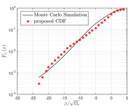
(a)

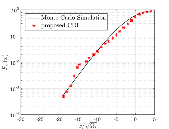
(b)

Figure 2: Fitting of GS-TWDP envelope CDF analytical expression to the empirical data measured in: (a) LOS scenario [21, Fig. 6 (LOS)] (b) NLOS scenario [21, Fig. 6 (NLOS)]

In Fig. 2, empirical CDFs generated form two different sets of measurements, performed in LOS and NLOS conditions, are compared to the best fitted CDFs generated using (21). Obviously, analytical CDF presented in Fig. 2, obtained for the following set of parameters: $K=15$, $\Gamma=0.5$ and $m=15$, provides extremely good fit to a given set of LOS measurement results, with the fitting error $\epsilon=0.22$. Similarly, analytically obtained CDF for a set of parameters $K=12$, $\Gamma=0.15$ and $m=2$ also provides excellent fit to the NLOS measurement results, with the error $\epsilon=0.24$.

Besides the aforesaid, it can be noticed that estimated parameters values which provide minimum fitting errors are also in accordance with underlying physical mechanisms. Namely, obtained parameters’ values for a LOS case reflect moderate amount of variations caused by multipath, while relatively large value of $m$, as expected in LOS conditions, indicates insignificant shadowing severity. On the country, in the NLOS conditions, parameter $m$ has very small value, which reflects propagation in which shadowing effect is pronounced, as it should be in case of a NLOS propagation.

IV Performance analysis

In order to demonstrate the applicability of obtained GS-TWDP statistical expressions for derivation of error performance metrics, in this section, ASEP of the M-ary RQAM modulation is considered. Thereat, M-ary RQAM is chosen as a technique frequently used these days in many wireless communication applications (such as microwave, high-speed mobile communication systems) [30], due to its simultaneous power and spectral efficiency.

Accordingly, for a considered modulation scheme, ASEP in GS-TWDP channel can be derived by averaging its conditional SEP in AWGN, $P_{e}(\gamma)$, over the GS-TWDP PDF given by (15):

$$P_{s}=\int_{0}^{\infty}P_{e}(\gamma)p_{\gamma}(\gamma)\mathop{}\!\mathrm{d}{\gamma}$$ (22)

where $P_{e}(\gamma)$ can be written as [30]:

$$P_{e}(\gamma)=2pQ\left(a\sqrt{\gamma}\right)+2qQ\left(b\sqrt{\gamma}\right)-4pqQ\left(a\sqrt{\gamma}\right)Q\left(b\sqrt{\gamma}\right)$$ (23)

and $Q(\cdot)$ is Gaussian Q-function, $p=1-1/M_{I}$, $q=1-1/M_{Q}$, $a=\left(6/\left(\left(M_{I}^{2}-1\right)+\beta^{2}\left(M_{Q}^{2}-1\right)\right)\right)^{0.5}$, $b=\beta a$ and $\beta$ is the ratio between quadrature and in-phase decision distances, i.e. $\beta=d_{Q}/d_{I}$, while modulation order $M$ is equal to $M=M_{I}\times M_{Q}$. Following [30], (22) could be calculated as the exact expression given in terms of a bivariate Meijer’s G function. However, these functions are very difficult to compute in common software packages. Accordingly, approximations of the involved Q-function could be used in order to provide easy-to-compute ASEP upper bound for M-ary RQAM modulation technique.

In these circumstances, Q-function can be approximated using Chernoff or Chiani approximations:

$$Q(x)\approx\frac{1}{2}e^{-\frac{x^{2}}{2}}$$ (24)

$$Q(x)\approx\frac{1}{12}e^{-\frac{x^{2}}{2}}+\frac{1}{4}e^{-\frac{2x^{2}}{3}}$$ (25)

respectively, which, after inserting in (23), provide the approximate M-ary RQAM conditional SEPs in AWGN is given by [30, eq. (12) and (15)]. These expressions then can be combined with (15) within the expression (22), and after some simple manipulations, expressed in term of the MGF (19), as:

$$\begin{split}P_{s,{Chernoff}}&\approx p\mathcal{M}_{\gamma}\left(\frac{a^{2}}{2}\right)+q\mathcal{M}_{\gamma}\left(\frac{b^{2}}{2}\right)\\ &-pq\mathcal{M}_{\gamma}\left(\frac{a^{2}+b^{2}}{2}\right)\end{split}$$ (26)

$$\begin{split}P_{s,{Chiani}}&\approx\frac{p}{6}\mathcal{M}_{\gamma}\left(\frac{a^{2}}{2}\right)+\frac{q}{6}\mathcal{M}_{\gamma}\left(\frac{b^{2}}{2}\right)\\ &-\frac{pq}{6}\mathcal{M}_{\gamma}\left(\frac{a^{2}+b^{2}}{2}\right)+\frac{p}{2}\mathcal{M}_{\gamma}\left(\frac{2a^{2}}{3}\right)\\ &+\frac{q}{2}\mathcal{M}_{\gamma}\left(\frac{2b^{2}}{3}\right)-\frac{pq}{2}\mathcal{M}_{\gamma}\left(\frac{2(a^{2}+b^{2})}{3}\right)\end{split}$$ (27)

i.e. as a close-form approximate ASEP expressions (28) and (29).

$$\begin{split}P_{s,{Chernoff}}&\approx e^{-K}\sum_{j=0}^{\infty}\frac{K^{j}t_{j}}{j!}\left(p\left(\frac{K+1}{\gamma_{0}}\frac{2m}{a^{2}}\right)^{m}U\left[m,m-j,\frac{K+1}{\gamma_{0}}\frac{2m}{a^{2}}\right]+q\left(\frac{K+1}{\gamma_{0}}\frac{2m}{b^{2}}\right)^{m}\right.\\ &\left.\times U\left[m,m-j,\frac{K+1}{\gamma_{0}}\frac{2m}{b^{2}}\right]-pq\left(\frac{K+1}{\gamma_{0}}\frac{2m}{a^{2}+b^{2}}\right)^{m}U\left[m,m-j,\frac{K+1}{\gamma_{0}}\frac{2m}{a^{2}+b^{2}}\right]\right)\end{split}$$ (28)

$$\begin{split}P_{s,{Chiani}}&\approx e^{-K}\sum_{j=0}^{\infty}\frac{K^{j}t_{j}}{j!}\left(\frac{p}{6}\left(\frac{K+1}{\gamma_{0}}\frac{2m}{a^{2}}\right)^{m}U\left[m,m-j,\frac{K+1}{\gamma_{0}}\frac{2m}{a^{2}}\right]+\frac{q}{6}\left(\frac{K+1}{\gamma_{0}}\frac{2m}{b^{2}}\right)^{m}U\left[m,m-j,\frac{K+1}{\gamma_{0}}\frac{2m}{b^{2}}\right]\right.\\ &\left.-\frac{pq}{6}\left(\frac{K+1}{\gamma_{0}}\frac{2m}{a^{2}+b^{2}}\right)^{m}U\left[m,m-j,\frac{K+1}{\gamma_{0}}\frac{2m}{a^{2}+b^{2}}\right]+\frac{p}{2}\left(\frac{K+1}{\gamma_{0}}\frac{3m}{2a^{2}}\right)^{m}U\left[m,m-j,\frac{K+1}{\gamma_{0}}\frac{3m}{2a^{2}}\right]\right.\\ &\left.+\frac{q}{2}\left(\frac{K+1}{\gamma_{0}}\frac{3m}{2b^{2}}\right)^{m}U\left[m,m-j,\frac{K+1}{\gamma_{0}}\frac{3m}{2b^{2}}\right]-\frac{pq}{2}\left(\frac{K+1}{\gamma_{0}}\frac{3m}{2(a^{2}+b^{2})}\right)^{m}U\left[m,m-j,\frac{K+1}{\gamma_{0}}\frac{3m}{2(a^{2}+b^{2})}\right]\right)\end{split}$$ (29)

V Numerical results

In this section, figures showing ASEPs for 4x2 RQAM versus average SNR are presented for different combinations of parameters $K$, $\Gamma$ and $m$, which correspond to a different composite fading channel conditions. Thereby, shown analytical results are obtained by direct evaluation of the expressions (28) and (29). Additionally, Monte Carlo simulated results are generated using $10^{5}$ random realizations following GS-TWDP distribution and are presented in order to validate derived analytical expressions.

Accordingly, from Fig. 4 - Fig. 8 can be observed that ASEP expression obtained by using Chiani approximation almost perfectly matches simulated results for all examined combination of GS-TWDP parameters, while derived expression obtained using Charnoff approximation provides the upper ASEP bound for a considered modulation.

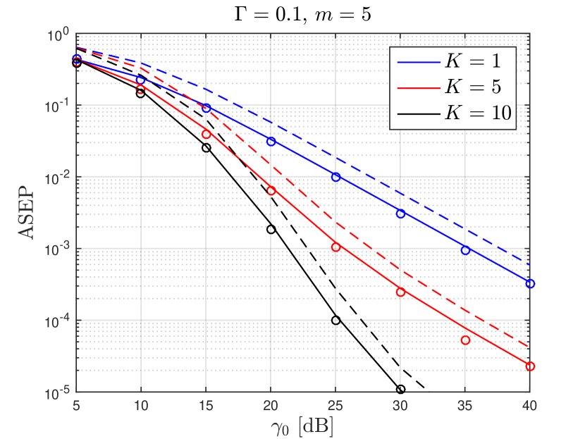
(a)

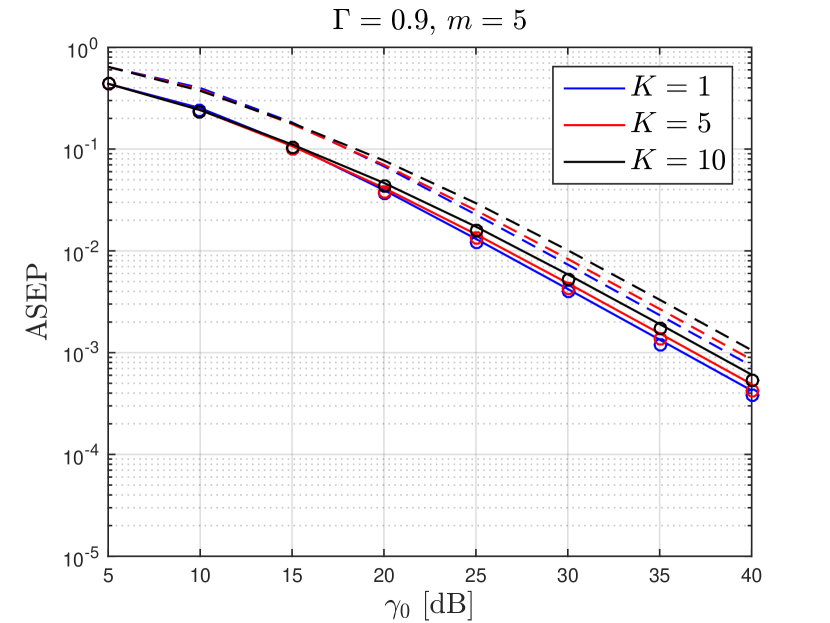
(b)

Figure 3: Chiani approximation (solid line), Chernoff approximation (dotted line), and Monte-Carlo simulation (dots) of 4x2 RQAM ASEP in a GS-TWDP fading channel for different values of $K$ and: (a) $\Gamma=0.1,m=5$, (b) $\Gamma=0.9,m=5$

(a)

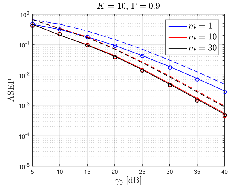
(b)

Figure 4: Chiani approximation (solid line), Chernoff approximation (dotted line), and Monte-Carlo simulation (dots) of 4x2 RQAM ASEP in a GS-TWDP fading channel for different values of $m$ and: (a) $K=10$, $\Gamma=0.1$, (b) $K=10$, $\Gamma=0.9$

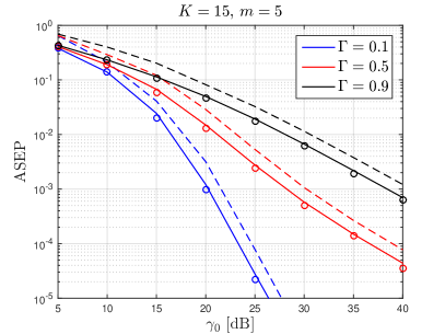
Figure 5: Chiani approximation (solid line), Chernoff approximation (dotted line), and Monte-Carlo simulation (dots) of 4x2 RQAM ASEP in a GS-TWDP fading channel for different values of $\Gamma$ ($K=15,m=5$)

Thereat, Fig. 4 - Fig. 6 show the impact of multipath severity on system performances, indicating similar behaviour of GS-TWDP to a TWDP model, for a fixed value of parameter $m$. Namely, for small values of $\Gamma$ (which correspond to a light multipath fading severity), increment in $K$ leads to performance improvements. On the contrary, for large $\Gamma$ close to 1 (i.e. when multipath is very severe), performance degrades with the increment of $K$. In addition, regardless the value of $K$, increment in $\Gamma$ leads to performance degradation.

On the contrary, Fig. 7 and Fig. 8 show the impact of shadowing severity on ASEP. Obviously, when specular and diffuse components experience lighter shadowing-caused fluctuations (expressed by large values of $m$), ASEP improves in respect to cases of shadowing described by small values of $m$. Thereat, in channels with severe multipath fluctuations (in which $K$ is large and $\Gamma\to 1$), multipath-caused variations dominates and shadowing-caused fluctuations have very small impact on error probability. On the contrary, when multipath-caused variations are less pronounced (i.e. when simultaneously $K$ is large and $\Gamma$ is small), the impact of shadowing on ASEP is much more significant and remarkably worsen performances in respect to those obtained in TWDP channels (for which $m\to\infty$). However, regardless the multipath fading severity, when $m$ increases above some value (e.g. $m>10$), shadowing effect on signal can be neglected, and overall performances are going to be pretty much identical to those in TWDP multipath channel.

VI Conclusion

In this paper, a novel composite fading model called GS-TWDP is introduced for modeling shadowing- and multipath-caused variation within the emerging mmWave bands. For a proposed model, corresponding PDF, CDF, n-th moment and MGF are derived as a closed-form expressions, given in terms of functions which can be easily evaluated using standard tools like MATLAB, Mathematica etc. The usability of derived expressions for evaluation of system performance metrics is demonstrated on the example of Chernoff- and Chiani-based M-ary RQAM ASEP upper bound expressions, which are also expressed in terms of a standardized mathematical function. Proposed model is, in addition, empirically verified by utilizing KS test and in literature reported measurement results at 28 GHz, which all make GS-TWDP inevitable candidate for modeling overall signal variations at mmWave frequencies.

References

- [1] D. W. Matolak and J. Frolik, “Worse-than-rayleigh fading: Experimental results and theoretical models,” IEEE Communications Magazine, vol. 49, no. 4, pp. 140–146, 2011.
- [2] T. Mavridis, L. Petrillo, J. Sarrazin, A. Benlarbi-Delaï, and P. De Doncker, “Near-body shadowing analysis at 60 GHz,” IEEE Transactions on Antennas and Propagation, vol. 63, no. 10, pp. 4505–4511, 2015.
- [3] G. D. Durgin, T. S. Rappaport, and D. A. de Wolf, “New analytical models and probability density functions for fading in wireless communications,” IEEE Transactions on Communications, vol. 50, no. 6, pp. 1005–1015, 2002.
- [4] S. Schwarz, E. Zöchmann, M. Müller, and K. Guan, “Dependability of directional millimeter wave vehicle-to-infrastructure communications,” IEEE Access, vol. 8, pp. 53 162–53 171, 2020.
- [5] E. Zöchmann, M. Hofer, M. Lerch, S. Pratschner, L. Bernadó, J. Blumenstein, S. Caban, S. Sangodoyin, H. Groll, T. Zemen, A. Prokeš, M. Rupp, A. F. Molisch, and C. F. Mecklenbräuker, “Position-specific statistics of 60 ghz vehicular channels during overtaking,” IEEE Access, vol. 7, pp. 14 216–14 232, 2019.
- [6] E. Zöchmann, S. Caban, C. F. Mecklenbräuker, S. Pratschner, M. Lerch, S. Schwarz, and M. Rupp, “Better than Rician: Modelling millimetre wave channels as two-wave with diffuse power,” EURASIP Journal on Wireless Communications and Networking, vol. 2019, no. 1, Jan. 2019.
- [7] J. M. Romero-Jerez, F. J. Lopez-Martinez, J. F. Paris, and A. J. Goldsmith, “The fluctuating two-ray fading model: Statistical characterization and performance analysis,” IEEE Transactions on Wireless Communications, vol. 16, no. 7, p. 4420–4432, Jul 2017.
- [8] I. M. Kostic, “Analytical approach to performance analysis for channel subject to shadowing and fading,” IEE Proceedings, vol. 152, no. 6, pp. 821–827, 2005.
- [9] A. Abdi and M. Kaveh, “On the utility of gamma pdf in modeling shadow fading (slow fading),” in 1999 IEEE 49th Vehicular Technology Conference (Cat. No.99CH36363), vol. 3, 1999, pp. 2308–2312 vol.3.
- [10] J. Liberti and T. Rappaport, “Statistics of shadowing in indoor radio channels at 900 and 1900 mhz,” in MILCOM 92 Conference Record, 1992, pp. 1066–1070 vol.3.
- [11] J. Weitzen and T. Lowe, “Measurement of angular and distance correlation properties of log-normal shadowing at 1900 mhz and its application to design of pcs systems,” IEEE Transactions on Vehicular Technology, vol. 51, no. 2, pp. 265–273, 2002.
- [12] T. S. Rappaport, Y. Xing, G. R. MacCartney, A. F. Molisch, E. Mellios, and J. Zhang, “Overview of millimeter wave communications for fifth-generation (5g) wireless networks—with a focus on propagation models,” IEEE Transactions on Antennas and Propagation, vol. 65, no. 12, pp. 6213–6230, 2017.
- [13] T. S. Rappaport, G. R. MacCartney, M. K. Samimi, and S. Sun, “Wideband millimeter-wave propagation measurements and channel models for future wireless communication system design,” IEEE Transactions on Communications, vol. 63, no. 9, pp. 3029–3056, 2015.
- [14] A. Abdi and M. Kaveh, “A comparative study of two shadow fading models in ultrawideband and other wireless systems,” IEEE Transactions on Wireless Communications, vol. 10, no. 5, pp. 1428–1434, 2011.
- [15] ——, “K distribution: an appropriate substitute for rayleigh-lognormal distribution in fading-shadowing wireless channels,” Electronics Letters, vol. 34, pp. 851–852, 1998.
- [16] I. M. Kostic, “Mgf for gamma-shadowed ricean fading channel,” European Transactions on Telecommunications, vol. 19, p. 155–159, 2008.
- [17] P. C. Sofotasios and S. Freear, “On the -/gamma composite distribution: A generalized multipath/shadowing fading model,” in 2011 SBMO/IEEE MTT-S International Microwave and Optoelectronics Conference (IMOC 2011), 2011, pp. 390–394.
- [18] J. M. Romero-Jerez, F. J. Lopez-Martinez, J. F. Paris, and A. Goldsmith, “The fluctuating two-ray fading model for mmwave communications,” in 2016 IEEE Globecom Workshops (GC Wkshps), 2016, pp. 1–6.
- [19] M. Lecci, P. Testolina, M. Polese, M. Giordani, and M. Zorzi, “Accuracy versus complexity for mmwave ray-tracing: A full stack perspective,” IEEE Transactions on Wireless Communications, vol. 20, no. 12, pp. 7826–7841, 2021.
- [20] C.-X. Wang, J. Bian, J. Sun, W. Zhang, and M. Zhang, “A survey of 5g channel measurements and models,” IEEE Communications Surveys Tutorials, vol. 20, no. 4, pp. 3142–3168, 2018.
- [21] M. K. Samimi, G. R. MacCartney, S. Sun, and T. S. Rappaport, “28 ghz millimeter-wave ultrawideband small-scale fading models in wireless channels,” in 2016 IEEE 83rd Vehicular Technology Conference (VTC Spring), 2016, pp. 1–6.
- [22] N. Y. Ermolova, “Capacity analysis of two-wave with diffuse power fading channels using a mixture of gamma distributions,” IEEE Communications Letters, vol. 20, no. 11, pp. 2245–2248, 2016.
- [23] A. Maric, E. Kaljic, and P. Njemcevic, “An alternative statistical characterization of TWDP fading model,” Sensors, vol. 21, no. 22, p. 7513, 2021.
- [24] P. Njemcevic, E. Kaljic, and A. Maric, “Moment-based parameter estimation for the -parameterized TWDP model,” Sensors, vol. 22, no. 3, p. 774, 2022.
- [25] A. P. Prudnikov, Y. A. Bryčkov, and O. I. Maričev, Integrals and Series Vol I Elementary Functions. Gordon and Breach Science Publishers, 1986.
- [26] I. S. Gradshteyn and I. M. Ryzhik, Table of Integrals, Series, and Products, 7th ed. Academic Press, 2007.
- [27] A. P. Prudnikov, Y. A. Bryčkov, and O. I. Maričev, Integrals and Series Vol II Special Functions. Gordon and Breach Science Publishers, 1992.
- [28] “Wolfram functions,” https://functions.wolfram.com/, "[Online; accessed October 2021]".
- [29] J. Zhang, W. Zeng, X. Li, Q. Sun, and K. P. Peppas, “New results on the fluctuating two-ray model with arbitrary fading parameters and its applications,” IEEE Transactions on Vehicular Technology, vol. 67, no. 3, pp. 2766–2770, 2018.
- [30] M. Bilim and N. Kapucu, “Average symbol error rate analysis of qam schemes over millimeter wave fluctuating two-ray fading channels,” IEEE Access, vol. 7, pp. 105 746–105 754, 2019.