HDNet: High-resolution Dual-domain
Learning for Spectral Compressive Imaging

Abstract

The rapid development of deep learning provides a better solution for the end-to-end reconstruction of hyperspectral image (HSI). However, existing learning-based methods have two major defects. Firstly, networks with self-attention usually sacrifice internal resolution to balance model performance against complexity, losing fine-grained high-resolution (HR) features. Secondly, even if the optimization focusing on spatial-spectral domain learning (SDL) converges to the ideal solution, there is still a significant visual difference between the reconstructed HSI and the truth. Therefore, we propose a high-resolution dual-domain learning network (HDNet) for HSI reconstruction. On the one hand, the proposed HR spatial-spectral attention module with its efficient feature fusion provides continuous and fine pixel-level features. On the other hand, frequency domain learning (FDL) is introduced for HSI reconstruction to narrow the frequency domain discrepancy. Dynamic FDL supervision forces the model to reconstruct fine-grained frequencies and compensate for excessive smoothing and distortion caused by pixel-level losses. The HR pixel-level attention and frequency-level refinement in our HDNet mutually promote HSI perceptual quality. Extensive quantitative and qualitative evaluation experiments show that our method achieves SOTA performance on simulated and real HSI datasets. Code and models are released at https://github.com/caiyuanhao1998/MST

1 Introduction

Hyperspectral images (HSIs) with more spectral bands can capture richer scene information and fixed wavelength imaging characteristics, which are used in image classification [28], object detection [46], and tracking [26, 14] widely.

Imaging systems with single 1D or 2D sensors take a long time to scan a scene for HSIs. They are not suitable for capturing dynamic scenes. Recently, the coded aperture snapshot spectral imaging (CASSI) system [20, 36, 37] can capture 3D HSI cubes at a real-time rate. CASSI exploits a coded aperture to modulate the HSI signal and compress it into a 2D measurement. Nonetheless, a core problem of the CASSI system is to recover the reliable and fine underlying 3D HSI signal from the 2D compressed images.

Traditional methods mainly regularize the reconstruction based on hand-crafted priors that delineate the structure of HSI. But manually adjusted parameters result in poor generalization. Inspired by the success of deep learning in image restoration, researchers began using convolutional neural networks (CNN) for HSI reconstruction. Some methods [24, 19, 23, 39] focus on self-attention learning in the spatial HSI domain, but they usually sacrifice feature resolution to cut down the computational complexity of non-local attention maps [24, 23]. These operations inevitably damage the spectral auto-correlation and information continuity. Inspired by the extensive exploration of pixel-level attention in high-level visual tasks [2, 18], we find that it is critical to elaborate high-resolution (HR) and fine-grained spectral-spatial attention for HSIs. However, although finer attention is undoubtedly beneficial for reconstructing HSI with rich spectral bands, capturing pixel-level perception for HSI with 28 spectral channels is far more challenging than 3-channel RGB images. It requires an optimal trade-off between model performance and resource costs.

Besides, existing learning-based methods [38, 24, 23, 11] for HSI reconstruction mainly focus on spatial-spectral domain learning (SDL), where the spectral representations are sparsely presented in the frequency domain. The equal treatment of each frequency may result in sub-optimal mode efficiency. Some works show that due to the inherent biases of CNNs [34, 30, 29, 25], models tend to preferentially fit low-frequency components that are easy to synthesize while losing high-frequency components. We visualize the spectra of reconstructed HSIs in the frequency domain in Fig. LABEL:fig:intro. We can see that even if previous methods based on SDL converge to the ideal solution, there is still an obvious frequency domain discrepancy between these reconstructed HSIs and ground truth. TSA-Net [23] loses high-frequency information and has observable checkerboard artifacts. DGSMP [11] deviates to a limited frequency area. The focal frequency loss [13] is proven to be effective in synthesizing fine frequency components, but its potential to narrow the frequency domain gap in HSI reconstruction still remains under-explored. We find that each frequency in the spectra is the statistical sum across all pixels in the HSI, so the frequency-level supervision can offer a new solution for global optimization. Experiments show that frequency domain learning (FDL) can compensate for excessive smoothing and distortion caused by pixel-level SDL.

Motivated by these meaningful findings, we propose a high-resolution dual-domain learning network, dubbed HDNet. Dual-domain supervision exhausts the model representation capacity within its spatial-spectral domain and frequency domain. On the one hand, in the spatial-spectral domain, we split the feature as HR spectral attention and HR spatial attention, and connect them in an efficient feature fusion (EFF) manner. The proposed fine-grained pixel-level attention avoids dimensionality collapse for high internal resolution. On the other hand, we use the Discrete Fourier Transform (DFT) to supervise the frequency distance between truth and reconstructed HSIs adaptively. Dynamic weighting mechanism makes the model concentrate high frequencies that are difficult to synthesize. Frequency spectra reconstructed by HDNet are the closest to the truth in Fig. LABEL:fig:intro, which shows our superiority in narrowing the frequency difference between HSIs. The HR pixel-level attention in SDL and frequency-level refinement in FDL mutually promote common prosperity and ameliorate image quality further. Specific contributions of this paper are:

• Dynamic frequency-level supervision that can narrow the frequency domain discrepancy is first used to improve the perceptual quality of HSIs. The proposed FDL forces the model to restore high and hard frequencies adaptively.

• We design the HR pixel-level attention in SDL for higher internal feature resolution, which further assists frequency alignment in FDL. Complementary dual-domain learning mechanism ameliorate HSI quality mutually.

• Our method achieves state-of-the-art (SOTA) performance in quantitative evaluation and visual comparison. Extensive experiments prove the superiority of HDNet.

2 Related Work

2.1 HSI Reconstruction

Traditional methods [16, 17, 36, 19, 40, 50, 49, 5] mainly recover the 3D HSI cube from the 2D compressive measurement based on hand-crafted priors. Nonetheless, these model-based methods suffer from poor generalization ability. Inspired by the success of deep learning, researchers have started using deep CNN for HSI reconstruction [24, 38, 39, 23, 11]. GAP-Net [22] presents a deep unfolding method and utilizes a pre-trained denoiser for HSI restoration. $\lambda$-Net [24] and TSA-Net [23] explores the self-attention for spatial features. The DGSMP [11] uses the deep Gaussian scale mixture prior for promising HSI reconstruction. However, current learning-based methods mainly focus on the spatial-spectral domain, where the frequency domain learning for HSI reconstruction remains under-investigated.

2.2 Self-Attention Mechanism

The self-attention mechanism [35, 32] is widely used to capture long-range interactions. Many attention module and its variants used for natural images have shown great potential [42, 10, 9, 33, 45]. The $\lambda$-Net [24] first explored the feature auto-correlation in HSI restoration. Then  [21] uses the bi-directional network to model spectral correlation. The TSA-Net [23] calculates the spatial attention map and the spectral attention map separately. Wang et al. [39] utilize the local and non-local correlation between spectral images. However, most existing networks sacrifice the internal resolution of attention to speed up calculations, which inevitably degrades performance. There are some pixel-level attention modules designed for high-level tasks [53, 2, 18] further enhances the model’s representation ability. Therefore, the exploration of pixel-level HR attention for HSI reconstruction can provide a targeted solution for boosting performance.

2.3 Image Frequency Spectrum Analysis

Frequency spectrum analysis describes signal frequency characteristics [34, 30]. The F-Principle [48] prove that deep learning networks tend to prefer low frequencies to fit the objective, which will result in the frequency domain gap [47, 52]. Recent studies [41, 51, 12] indicate that the periodic pattern shown in the frequency spectrum may be consistent with the artifacts in the spatial domain. Therefore, some works try to reduce the visual difference by narrowing the frequency domain gap between the input and output. [6] treats low-frequency and high-frequency images differently during training. DASR [44] uses domain-gap aware training and domain-distance weighted supervision to solve the domain deviation in super-resolution. Jiang et al. [13] proved that focusing on difficult frequencies can improve the reconstruction quality. In HSI reconstruction, the model over-fitting at low frequencies brings smooth textures and blurry structures. So exploring adaptive constraints on specific frequencies is essential for the refined reconstruction.

3 The Proposed Method

3.1 Overall Architecture

The overall network architecture and internal module details of our proposed HDNet are shown in Fig. LABEL:overall. We choose ResNet [7] as the baseline to build the proposed HDNet for a lightweight model, which is convenient to show the superiority of our designed plug-and-play components.

In CASSI, the mask $\textbf{m}\in\mathbb{R}^{H\times W}$ is used to modulate the HSI signals. Then the modulated HSIs are shifted in the dispersion process. Thus, we shift back the measurement $\textbf{y}\in\mathbb{R}^{H\times(W+d(N_{\beta}-1))}$, where $d$ denotes the shifting interval and $N_{\beta}$ denotes the number of wavelengths in HSIs. Then we formulate the dispersion process as follow:

$$\textbf{y}^{\prime}(x,y,n_{\beta})=\textbf{y}(x,y-d(\beta_{n}-\beta_{r})),$$ (1)

where $\textbf{y}^{\prime}$ represents the multi-channel shifted version of the measurement, $n_{\beta}\in\{1,...,N_{\beta}\}$ indices the spectral channel, $\beta{r}$ is supposed to the reference wavelength, and $d(\beta_{n}-\beta_{r})$ indicates the shifted distance for the $n_{\beta}$-th channel. Then we use the mask to modulate $\textbf{y}^{\prime}$ for the input:

$$\textbf{x}_{in}=\textbf{y}^{\prime}\odot\textbf{m},$$ (2)

where $\odot$ denotes the element-wise product. Then we define the $3\times 3$ convolution layer as ${F}_{conv}^{3\times 3}(\cdot)$ to extract shallow features, and the corresponding features $\textbf{x}_{0}$ is defined as:

$$\textbf{x}_{0}={F}_{conv}^{3\times 3}(\textbf{x}_{in}).$$ (3)

To prove the effectiveness and efficiency of the spatial-spectral domain learning module, we only insert an SDL block in the middle of the stacked residual blocks (RBs). We define the number of RB stacked before and after SDL as $l$ and $g$ respectively, and we process the input as follow:

$$\begin{split}\textbf{x}_{t}&={F}^{l}_{RB}(\textbf{x}_{l-1})={F}^{l}_{RB}({F}^{l-1}_{RB}(\cdot\cdot\cdot({F}^{1}_{RB}(\textbf{x}_{0}))\cdot\cdot\cdot)),\\ \hat{\textbf{x}}_{f}&={F}_{SDL}(\textbf{x}_{t}),\\ \hat{\textbf{x}}_{t}&={F}^{g}_{RB}(\textbf{x}_{g-1})={F}^{g}_{RB}({F}^{g-1}_{RB}(\cdot\cdot\cdot({F}^{1}_{RB}(\hat{\textbf{x}}_{f}))\cdot\cdot\cdot)),\end{split}$$ (4)

where the ${F}_{RB}(\cdot)$ and ${F}_{SDL}(\cdot)$ correspond to the RB and SDL module functions. The SDL module includes HR spectral attention, HR spatial attention, and efficient feature fusion (EFF). The internal implementation details of these modules will be described in Section 3.2. To maintain the high internal resolution of the features extracted from the stacked RBs, we use feature reshape and matrix multiplication operations instead of feature downsampling and channel sharp narrowing operations, and the grouped split-and-merge structure is designed for efficient feature fusion.

Global skip connection combines the shallow features $\textbf{x}_{0}$ with the deep features to further increase the model stability and information flow. Through the channel adjustment of the convolutional layers, we get the reconstructed HSI as:

$$y_{pred}={F}_{conv}^{3\times 3}({F}_{conv}^{3\times 3}(\hat{\textbf{x}}_{t})+\textbf{x}_{0}).$$ (5)

As shown in Fig. LABEL:overall, the predicted HSI $y_{pred}$ is supervised by a dual-domain learning mechanism. The SDL module is designed to be plug-and-play, and the FDL mechanism is used for loss optimization, which constrains the frequency distance between the reconstructed HSI and the truth adaptively. Dynamic weighting mechanism makes the model focus on hard frequencies reconstruction that is easily ignored by SDL. The HR pixel-level attention in SDL and the frequency-level refinement in FDL to achieve complementary learning, which further ameliorates HSI quality. In the following, we will introduce these two domains in detail.

3.2 Spatial-Spectral Domain Learning

We extract the HR spatial-spectral attention cross spectral and spatial direction respectively, and perform efficient feature fusion (EFF) for more efficient representation.

HR Spectral Attention. We use two convolution layers to obtain query vector defined as $f_{c}^{q}$ with the full spatial resolution and key vector defined as $f_{c}^{k}$ with the half channel resolution. Then the query vector does attention remapping to the key vector for the value vector $f_{c}^{v}$, and its spectral dimension remains $C/2$, which avoids excessive loss of continuity. The the input $\textbf{x}_{t}\in\mathbb{R}^{\it H\times\it W\times\it C}$ is processed as:

$$\begin{split}f_{c}^{q}&={F}_{conv}^{1\times 1}(\textbf{x}_{t})\in\mathbb{R}^{\it 1\times\it H\times\it W},\\ f_{c}^{k}&={F}_{conv}^{1\times 1}(\textbf{x}_{t})\in\mathbb{R}^{\textit{C / }2\times\it H\times\it W},\\ f_{c}^{v}&={F}_{R}(f_{c}^{k})\otimes Softmax[{F}_{R}(f_{c}^{q})]\in\mathbb{R}^{\textit{C / }2\times\it 1\times\it 1},\end{split}$$ (6)

where ${F}_{conv}^{1\times 1}(\cdot)$ is the $1\times 1$ convolution function and the reshape function ${F}_{R}(\cdot)$ is used to facilitate size matching. $\otimes$ means matrix multiplication operation. In Fig. LABEL:overall, after channel adjustment and Sigmoid activation, the weight factor of each channel can be obtained. Then the original feature $\textbf{x}_{t}$ is re-calibrated through channel element-wise product operation for HR spectral attention feature $\textbf{x}_{spe}$, defined as:

$$\textbf{x}_{spe}=\textbf{x}_{t}\odot{F}_{conv}^{1\times 1}(Sigmoid[f_{c}^{v}]).$$ (7)

HR Spatial Attention. For the input $\textbf{x}_{t}\in\mathbb{R}^{\it H\times\it W\times\it C}$, we obtain the key vector defined as$f_{s}^{k}$ with the half channel resolution and the full spatial resolution. The query vector defined as $f_{s}^{q}$ is regarded as the remapping factor to adjust the spatial attention for the value vector $f_{s}^{v}$. Even if the global average pooling (GAP) sacrifices the channel resolution of $f_{s}^{q}$, the full spatial resolution of $f_{s}^{v}$ will bring HR features in the spatial dimension. These operations are defined as:

$$\begin{split}f_{s}^{q}&={F}_{GAP}({F}_{conv}^{1\times 1}(\textbf{x}_{t}))\in\mathbb{R}^{\textit{1}\times\textit{1}\times{\textit{C / }}2},\\ f_{s}^{k}&={F}_{conv}^{1\times 1}(\textbf{x}_{t})\in\mathbb{R}^{\textit{C / }2\times\it H\times\it W},\\ f_{s}^{v}&=Softmax[{F}_{R}(f_{s}^{q})]\otimes{F}_{R}(f_{s}^{k})\in\mathbb{R}^{\it 1\times\it HW},\end{split}$$ (8)

where ${F}_{GAP}(\cdot)$ is the GAP function. As shown in Fig. LABEL:overall, we re-calibrate the original feature $\textbf{x}_{t}$ by the weight factor of each spatial feature coordinate, and these weight factors come from the Sigmoid activation value of $f_{s}^{v}$. Then the HR spatial attention feature $\textbf{x}_{spa}$ is calculated as:

$$\textbf{x}_{spa}=\textbf{x}_{t}\odot Sigmoid[{F}_{R}(f_{s}^{v})].$$ (9)

Efficient Feature Fusion. To further improve the feature utilization and interactivity within the spectral-spatial attention learning, we use an efficient fusion manner to group and re-interact the input features. Firstly, we fuse the spectral attention feature $\textbf{x}_{spe}$ and spatial attention feature $\textbf{x}_{spa}$:

$$\textbf{x}_{f}=\textbf{x}_{spe}+\textbf{x}_{spa},$$ (10)

where $\textbf{x}_{f}\in\mathbb{R}^{\rm H\times W\times C}$. Then, considering the diverse importance of different channels, we divide feature $\textbf{x}_{f}$ into $m$ groups, so the $\textbf{x}_{f}$ can be expressed as $[\textbf{x}_{f}^{1},\textbf{x}_{f}^{2},\textbf{x}_{f}^{3},...,\textbf{x}_{f}^{m}]$. The channel number of each group $\textbf{x}^{i}_{f}$ ($i\in[1,m]$) is $C/m$.

As shown in Fig. LABEL:overall, we replace the standard convolution with the depthwise-separable convolution (DSC) [31, 8, 4] to reduce the computational cost. For each group of features $\textbf{x}^{i}_{f}$, the salient features are extracted independently. After activating through the Softmax layer, the corresponding weighting factor ${f}^{i}_{e}$ of each group can be expressed as:

$$\begin{split}{f}^{i}_{e}&={F}_{DSC}(\textbf{x}^{i}_{f})\\ &=Softmax[{F}_{conv}^{PWC}(F_{MP}({F}_{conv}^{DWC}(\textbf{x}^{i}_{f})))],\end{split}$$ (11)

where ${F}_{conv}^{PWC}(\cdot)$ is the point-wise convolution (PWC), and ${F}_{conv}^{DWC}(\cdot)$ represents the depth-wise convolution (DWC). The $F_{MP}(\cdot)$ represents the max pooling function with a kernel size of $3\times 3$. The normalized weight ${f}^{i}_{e}$ re-calibrates $\textbf{x}^{i}_{f}$. Then we introduce residual skip connection to further promote information flow. and get the re-interaction feature as:

$$\hat{\textbf{x}}^{i}_{f}={f}^{i}_{e}\textbf{x}^{i}_{f}+\textbf{x}^{i}_{f}.$$ (12)

We traverse each group and connect the feature maps of each group to obtain the final fusion feature $\hat{\textbf{x}}_{f}$ as follows:

$$\hat{\textbf{x}}_{f}=[\hat{\textbf{x}}^{1}_{f},\hat{\textbf{x}}^{2}_{f},\hat{\textbf{x}}^{3}_{f},...,\hat{\textbf{x}}^{m}_{f}],$$ (13)

where $[\cdot]$ denotes the concatenating operation. The efficient grouped DSC adjusts feature interactions of each group dynamically instead of equal treatment, which further ensures the extraction of high-resolution features. Efficient calculation greatly reduces parameter cost and calculation burden.

3.3 Frequency Domain Learning

The inherent bias of CNN makes it challenging to synthesize high-frequency features in SDL, which leads to the frequency domain discrepancy in other methods in Fig.LABEL:fig:intro. so we introduce dynamic FDL for frequency-level supervision.

Discrete Fourier Transform. DFT transforms the discrete signal from the time domain to the frequency domain to analyze the frequency structure. For a finite-length discrete 1D signal, the sine wave components of each frequency are obtained through the following correspondence:

$$F(w)=\textstyle\frac{1}{N}\sum_{n=0}^{N-1}f(n)e^{-j2\pi{\frac{wn}{N}}},$$ (14)

where $F(w)$ represent the frequency domain signal corresponding to the 1D discrete time domain signal $f(n)$.

HSI Frequency Spectra Analysis. We use the 2D DFT to convert the HSI to the frequency domain to reconstruct more high-frequency details. We define the ground truth and reconstructed HSI as $y_{gt}$ and $y_{pred}$ with the dimensions of $\mathbb{R}^{\it H\times W\times C}$. We calculate the frequency spectrum for each channel. In a specific channel $k$, the conversion relationship between spatial coordinates $(h,w,k)$ and frequency domain coordinates $(u,v)$ is expressed as:

$$\begin{split}\textbf{F}^{k}_{gt}(u,v)&=\textstyle{\sum_{h=0}^{H-1}}{\sum_{w=0}^{W-1}}y_{gt}(h,w,k)e^{-j2\pi({\frac{uh}{H}}+{\frac{vw}{W}})},\\ \textbf{F}^{k}_{pred}(u,v)&=\textstyle{\sum_{h=0}^{H-1}}{\sum_{w=0}^{W-1}}y_{pred}(h,w,k)e^{-j2\pi({\frac{uh}{H}}+{\frac{vw}{W}})},\\ \end{split}$$ (15)

where the $\textbf{F}_{gt}$ and $\textbf{F}_{pred}$ are the frequency spectra of all channels corresponding to $y_{gt}$ and $y_{pred}$. As shown in Fig. LABEL:overall, their frequency spectra visualization represents the severity of the grayscale changes. The structural textures and edges are mapped as high-frequency signals while the background as low-frequency signals. Therefore, we can easily manipulate the high-frequency or low-frequency information of the HSI. Then we introduce dynamic weights to make the network treat different frequencies adaptively.

Method	TwIST [1]	GAP-TV [49]	DeSCI [19]	$\lambda$-Net [24]	HSSP [38]	DNU [39]	TSA-Net [23]	DGSMP [11]	HDNet (Ours)
Scene1	25.16, 0.6996	26.82, 0.7544	27.13, 0.7479	30.10, 0.8492	31.48, 0.8577	31.72, 0.8634	32.03, 0.8920	33.26, 0.9152	34.95, 0.9478
Scene2	23.02, 0.6038	22.89, 0.6103	23.04, 0.6198	28.49, 0.8054	31.09, 0.8422	31.13, 0.8464	31.00, 0.8583	32.09, 0.8977	32.52, 0.9531
Scene3	21.40, 0.7105	26.31, 0.8024	26.62, 0.8182	27.73, 0.8696	28.96, 0.8231	29.99, 0.8447	32.25, 0.9145	33.06, 0.9251	34.52, 0.9569
Scene4	30.19, 0.8508	30.65, 0.8522	34.96, 0.8966	37.01, 0.9338	34.56, 0.9018	35.34, 0.9084	39.19, 0.9528	40.54, 0.9636	43.00, 0.9810
Scene5	21.41, 0.6351	23.64, 0.7033	23.94, 0.7057	26.19, 0.8166	28.53, 0.8084	29.03, 0.8326	29.39, 0.8835	28.86, 0.8820	32.49, 0.9565
Scene6	20.95, 0.6435	21.85, 0.6625	22.38, 0.6834	28.64, 0.8527	30.83, 0.8766	30.87, 0.8868	31.44, 0.9076	33.08, 0.9372	35.96, 0.9645
Scene7	22.20, 0.6427	23.76, 0.6881	24.45, 0.7433	26.47, 0.8062	28.71, 0.8236	28.99, 0.8386	30.32, 0.8782	30.74, 0.8860	29.18, 0.9373
Scene8	21.82, 0.6495	21.98, 0.6547	22.03, 0.6725	26.09, 0.8307	30.09, 0.8811	30.13, 0.8845	29.35, 0.8884	31.55, 0.9234	34.00, 0.9609
Scene9	22.42, 0.6902	22.63, 0.6815	24.56, 0.7320	27.50, 0.8258	30.43, 0.8676	31.03, 0.8760	30.01, 0.8901	31.66, 0.9110	34.56, 0.9576
Scene10	22.67, 0.5687	23.10, 0.5839	23.59, 0.5874	27.13, 0.8163	28.78, 0.8416	29.14, 0.8494	29.59, 0.8740	31.44, 0.9247	32.22, 0.9500
Average	23.12, 0.6694	24.36, 0.6993	25.27, 0.7207	28.53, 0.8406	30.35, 0.8524	30.74, 0.8631	31.46, 0.8939	32.63, 0.9166	34.34, 0.9572

Table 1: The PSNR in dB (left entry in each cell) and SSIM (right entry in each cell) results of the test methods on 10 scenes.

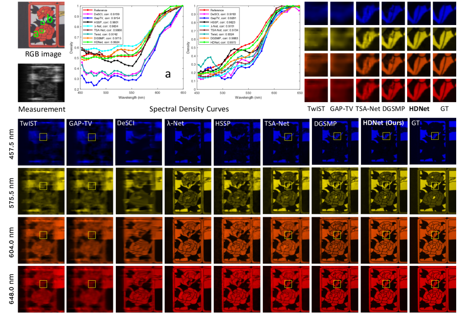
Figure 3: Simulated HSI reconstruction comparisons of Scene 7 with 4 (out of 28) spectral channels. We show the spectral curves (top-medium) corresponding to the selected green boxes of the RGB image. Our HDNet reconstructs more visually pleasant detailed contents.

Frequency Distance Optimization. We use a frequency distance coefficient $\alpha$ to make the distance correlation adjustable. In each channel $k$, the frequency distance between ground truth and predicted HSI is equivalent to the power distance between their spectrum, which is defined as:

$$d^{k}(u,v) =\textstyle{\|\textbf{F}^{k}_{gt}(u,v)-\textbf{F}^{k}_{pred}(u,v)\|}^{\alpha}.$$ (16)

The analysis of frequency-distance coefficients $\alpha$ is provided in Sec. 4.3. Then we define a dynamic weight factor $\theta(u,v)$ linearly related to the distance $d(u,v)$ to make the model pay more attention to the frequencies hard to be synthesized. Then the distance between the ground truth and the predicted HSI in a single channel $k$ is formulated as:

$$d(\textbf{F}_{gt}^{k},\textbf{F}_{pred}^{k}) =\textstyle{\frac{1}{HW}}{\sum_{u=0}^{H-1}}{\sum_{v=0}^{W-1}}\theta^{k}(u,v)d^{k}(u,v),$$ (17)

where the $\theta^{k}(u,v)$ changes linearly with the absolute value of the $k$-th channel frequency distance $\sqrt{(|d^{k}(u,v)|)}$. We traverse $k=\{0,1,2,...,C-1\}$ and sum each spectral distance to calculate the frequency domain loss in FDL as:

$$L_{FDL}(\textbf{F}_{gt},\textbf{F}_{pred}) =\textstyle{\sum_{k=0}^{C-1}}d(\textbf{F}_{gt}^{k},\textbf{F}_{pred}^{k}).$$ (18)

3.4 Traning Objective

We choose the least absolute error as the loss in SDL, i.e. ${L}_{SDL}(y_{gt},y_{pred})=\|y_{gt}-y_{pred}\|^{1}$. The loss in FDL is $L_{FDL}(\textbf{F}_{gt},\textbf{F}_{pred})$ defined in Eq. (18). We introduce the weight factor $\lambda$ to balance SDL and FDL, and the total loss combined with the dual-domain learning is expressed as:

$$L_{total} =\textstyle L_{SDL}(y_{gt},y_{pred})+\lambda L_{FDL}(\textbf{F}_{gt},\textbf{F}_{pred}).$$ (19)

It is worth mentioning that how the model focuses on hard frequencies in FDL can be controlled by $\alpha$ in Eq. (16). The larger $\alpha$, the greater the penalty for the hard frequencies.

4 Experiments

4.1 Experimental Setup

Datasets. We conduct experiments on two publicly available simulated HSI datasets CAVE [27] and KAIST [3] for a fair comparison. The CAVE consists of 32 HSIs with 31 spectral bands with a spatial size of 512$\times$512, and the KAIST consists of 30 HSIs with 31 spectral channels at a size of 2704$\times$3376. Following TSA-Net [23] and DGSMP [11], we use the same mask at a size of 256$\times$256 for simulation. 28 wavelengths ranging from 450nm to 650nm obtained by spectral interpolation manipulation are adopted. As with TSA-Net [23], we use the CAVE dataset for training and select 10 scenes from KAIST for testing.

Implementation Details. We follow the same experimental settings as TSA-Net [23]. During the training, a patch at the size of 256$\times$256$\times$28 is randomly selected from the training 3D HSI datasets as labels. After mask modulation, the data cube is shifted in spatial with an accumulative two-pixel step and then summed up along the spectral dimension to generate the 2D measurement of size 256$\times$310. Random flipping and rotation are used for data argumentation. We use 32 RBs ($l=g=$16) and insert one SDL module in the middle. We set $\alpha=2$ in Eq. (16) and $\lambda=0.7$ in Eq. (19). The HDNet is optimized by ADAM [15] with the learning rate of $4\times 10^{-4}$, which decreases linearly to half every 50 epochs. Our models are trained on NVIDIA GeForce RTX 2080 Ti GPU. Peak-signal-to-noise-ratio (PSNR) and structured similarity (SSIM) [43] are adopted as the metrics to evaluate the HSI reconstruction quantitatively.

4.2 Comparison with Other Methods

Quantitative Comparison: We compare the HSI reconstruction of the proposed HDNet with 7 other SOTA methods, including three conventional methods (TwIST [1], GAP-TV [49], and DeSCI [19]) and four CNN-based methods ($\lambda$-Net [24], HSSP [38], DNU [39], TSA-Net [23], and DGSMP [11]). The quantitative results on 10 scenes of the KAIST dataset in terms of PSNR and SSIM are reported in Tab. 1. We can see that our HDNet significantly outperforms other methods. Specifically, our method surpasses the recent best competitor DGSMP by 1.71 dB in average PSNR and 0.0406 in average SSIM. When compared with the two deep unfolding algorithms HSSP and DNU, our HDNet is 3.99 dB and 3.60 dB higher, respectively. When compared with the two model-based methods TwIST and DeSCI, our HDNet achieves 11.22 dB and 9.98 dB performance gain. Noted that although our HDNet’s PSNR is slightly lower than DGSMP in Scene7, SSIM exceeds it by a large margin, which proves that the frequency domain optimization strategy we use is more focused on the refinement of perceptual quality and structural similarity. The complementary spatial-spectral domain and frequency domain further improve the reconstruction performance.

Visual Comparison: We show the simulated HSI reconstruction comparisons of Scene 7 with 4 (out of 28) spectral channels in Fig. 3. The density-wavelength spectral curves correspond to the green boxes identified as $a$ and $b$ of the RGB image. We calculate the curve correlation between all comparison methods and the reference truth. These quantitative results show that our reconstructed HSI is the closest and highest correlation to the ground truth (GT). Besides, we visualize the entire HSI and enlarge the selected yellow boxes in the upper right of Fig. 3. Our HDNet generates more visually pleasant results than previous methods, especially in the reconstruction of high-frequency structural content and spectral-dimension consistency, which benefit from pixel-level and frequency-level dual-domain learning.

4.3 Ablation Study

Model Analysis. There are some existing attention networks used for HSI reconstruction. We reports their parameters, spatial resolution, model complexity, and performance in Tab. LABEL:attentional-mechanism. Noted that we retrain attentions in $\lambda$-Net [24] and TSA-Net [23] with the same baseline and the loss in Eq. (19) for a fair comparison. Although the $\lambda$-Net treats each channel equally, the non-local spatial mechanism makes its parameter amount as high as 62.64M. TSA-Net sacrifices part of the channel resolution in exchange for computation complexity, but the used spatial-spectral self-attention also has a higher parameter burden. Our HDNet achieves the best trade-off between model performance and parameters, and it also maintains the greatest fine details and resolutions in both channel resolution (CR) and spatial resolution (SR). The parameter of our HDNet is 2.37M, which is less than one-eighteenth of TSA-Net while maintaining the same model complexity. These results show the superiority of our proposed HR attention mechanism.

Attention Feature Visualization: To show the advantages of our proposed HR spatial-spectral attention (HSA) in capturing HR fine-grained features more intuitively, we visualize the intermediate attention maps of different attention modules used for HSI reconstruction. We take ResNet [7] as the baseline, and then add the TSA and our HSA, respectively. The corresponding results are shown in Fig. 4. Compared with the baseline, both TSA and HSA can enhance the extraction of salient features. However, TSA with lower resolution attention inevitably loses a lot of textures and edges and even focuses on the background by mistake. Our proposed HSA solves this problem well. The continuous HR attention in HSA allows the network to retain more high-frequency information and complete structure of HSI.

Loss Weight Factor. The weight factor $\lambda$ in Eq. (19) is introduced to adjust the importance of SDL and FDL dynamically. We analyze how the model performance changes with $\lambda$, and report the corresponding results in Tab. 3. $\lambda=0$ means that the model only minimizes the spatial-spectral domain loss, and its unsatisfactory results indicate that frequency-level supervision is necessary. It can be seen that as the proportion of FDL loss increases, the model performance also increases. When $\lambda=0.7$, the model performance reaches the highest PSNR and SSIM performance. The performance degradation caused by the continued increase of $\lambda$ indicates that excessive constraints on the frequency will destroy the pixel-level optimization balance.

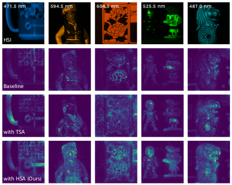
Figure 4: Feature visualization with different attention modules.

FDL Loss Ablation. We calculate the log frequency distance (LFD) as a frequency-level metric to evaluate the spectrum difference between the reconstructed HSI and truth. The LFD has a logarithmic relationship with the frequency distance $d(u,v)$ in Eq. (16), which is calculated as:

$$F_{LFD}=\textstyle log\Big{[}{\frac{1}{HW}}\Big{(}{\sum_{u=0}^{H-1}}{\sum_{v=0}^{W-1}}{|d(u,v)|}\Big{)}+1\Big{]}.$$ (20)

As shown in Fig. LABEL:fig:dfl, we visualize the 3D-spectra reconstructed with or without the FDL loss and provide the corresponding LFD. It can be seen that the reconstructed frequency 3D-spectra without frequency supervision has a ringing artifact, which will produce oscillations at the sharp brightness changes. Amplitude and phase distortion make different frequency components of HSI have different gain amplitude and relative displacement, which is manifested as deformed structure and color deviation in HSI. On the contrary, the 3D-spectra optimized with our proposed loss in FDL allow for more accurate frequency reconstruction and lower LFD, fitting the frequency statistics closer to truth. Fine-grained spectrum supervision further preserves more high-frequency information that is difficult to synthesize.

$\lambda$	0	0.1	0.3	0.5	0.7	0.9	1
SSIM $\uparrow$	0.9093	0.9369	0.9498	0.9538	0.9572	0.9425	0.9399
PSNR $\uparrow$	31.91	33.27	33.86	34.05	34.34	33.75	33.52

Table 3: Performance comparisons of different loss weight factor.

Metric	$\alpha$ = 0.1	$\alpha$ = 0.3	$\alpha$ = 0.5	$\alpha$ = 1	$\alpha$ = 2	$\alpha$ = 3
LFD $\downarrow$	14.8633	14.3792	13.9825	13.6571	13.3238	15.0863
SSIM $\uparrow$	0.9397	0.9428	0.9543	0.9569	0.9572	0.9065
PSNR $\uparrow$	33.16	33.51	34.14	34.40	34.34	31.89

Table 4: Model performance comparison using different coefficients to calculate the spectrum distances in frequency domain.

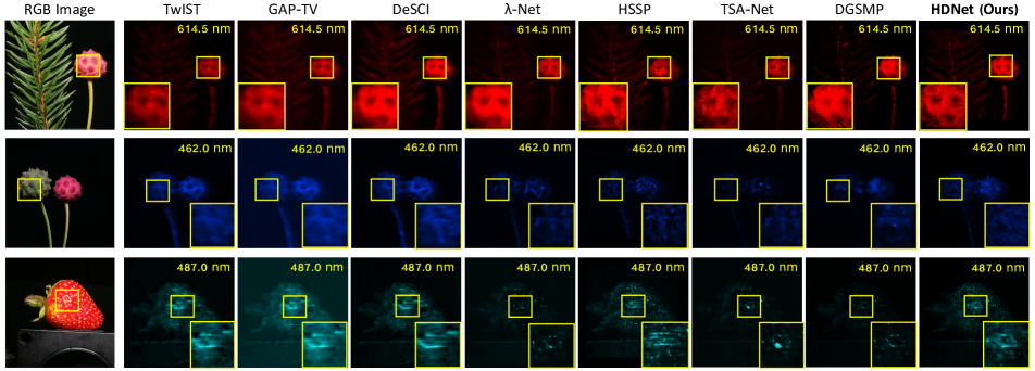
Figure 6: Real HSI reconstruction comparison of a randomly selected channel from 3 scenes. HDNet restores more high-frequency details.

Frequency Distance Coefficient. The far frequency distance between reconstructed HSI and truth represents the inaccurate fit, so we introduce a frequency distance coefficient $\alpha$ in Eq. (16) to control the model’s focus on frequencies that have not been reconstructed well. The larger $\alpha$ is, the greater the model will penalize the underfitting frequency. We report the model performance corresponding to different coefficients in Tab. 4. When $\alpha=1$, the model obtains the highest PSNR, and when $\alpha=2$, the model obtains the best SSIM and LFD performance. Smaller $\alpha$ results in weaker frequency penalty and slightly lower performance, but the larger $\alpha$ brings more stringent FDL supervision and excessive constraint, which will lead to HSI distortion and performance degradation. In order for the model to focus on both structural similarity and perceptual quality, we set $\alpha=2$ to balance the visual and quantitative results.

Metric	$p$ = 1	$p$ = 2	$p$ = 3	$p$ = 4	$p$ = 5	$p$ = 6
LFD $\downarrow$	14.7954	14.6287	13.3238	13.5982	14.6391	14.9625
SSIM $\uparrow$	0.9193	0.9344	0.9572	0.9378	0.9304	0.9166
PSNR $\uparrow$	32.96	33.29	34.34	33.69	33.15	32.67

Table 5: Model performance comparisons of different patch size.

Patch-based Frequency Spectrum. To further analyze the frequency characteristics of HSI, we replace the entire image spectrum calculation with patch-based calculation. The original HSI is cropped into $p\times p$ patches. The new frequency domain distance $\hat{L}_{FDL}(F_{gt},F_{pred})$ of each paired images will be redefined as the average value of each paired patches in the current channel. The Eq. (18) is modified as:

$$\hat{L}_{FDL}(F_{gt},F_{pred}) =\textstyle{\sum_{k=0}^{C-1}}[\frac{1}{p^{2}}{\sum_{j=1}^{p^{2}}}d(F_{gt}^{kj},F_{pred}^{kj})].$$ (21)

We analyze the performance when $p=\{1,2,3,4,5,6\}$ in Tab. 5 and visualize part of the spectra in Fig. LABEL:fig:patch_vis. The smaller patch-based subdivision brings a finer spectrum reconstruction, and the performance on narrowing the frequency domain gap shown by LFD also becomes better. However, the HSI reconstruction worsens when $p>3$. The visualization of $p=4$ in Fig. LABEL:fig:patch_vis shows that a too small patch brings limited spectrum representation and biased supervision. So we set $p=3$ to appropriately ameliorate the refinement of HSI.

4.4 Real HSI Reconstrcution

We also apply the proposed HDNet for real HSI reconstruction. The dataset is collected by the real HSI system designed in TSA-Net [23]. Each HSI has 28 spectral channels with wavelengths ranging from 450nm to 650nm and has 54-pixel dispersion in the column dimension. The measurement used as input is at a spatial size of 660$\times$714. Following TSA-Net [23], we re-train the HDNet with the real mask on the CAVE and KAIST datasets jointly. We also inject 11-bit shot noise on the 2D compressive image to simulate the real situations. Due to the lack of ground truth, we only compare the qualitative results of our HDNet with other methods. Reconstruction results of one channel randomly selected from 3 real scenes are shown in Fig. 6. Previous methods with only coarse spatial domain loss produce excessive smoothing and distortion of high-frequency details. The proposed HDNet generates more visually pleasant results by recovering more HR structures and high-frequency textures, which benefits from the pixel-level fine-grained and frequency-level refinement. Our robust results in the real dataset show good model generalization.

5 Conclusion

In this paper, we propose a high-resolution dual-domain learning network (HDNet) that includes spatial-spectral domain learning and frequency domain learning for HSI reconstruction from compressive measurements. The fine-grained pixel-level prediction is obtained by efficiently designing the HR spatial-spectral attention and feature fusion module. To solve the visual difference caused by the pixel-level loss, we introduce dynamically adjusted frequency-level supervision for the first time to narrow the frequency domain discrepancy between reconstructed HSI and the truth. HDNet exhausts the representation capacity within the dual-domain. Extensive visual analysis and quantitative experiments prove that the HDNet obtains superior results in both pixel-level and frequency-level HSI reconstruction.

References

- [1] J.M. Bioucas-Dias and M.A.T. Figueiredo. A new twist: Two-step iterative shrinkage/thresholding algorithms for image restoration. TIP, 2007.
- [2] Bowen Cheng, Maxwell D Collins, Yukun Zhu, Ting Liu, Thomas S Huang, Hartwig Adam, and Liang-Chieh Chen. Panoptic-deeplab: A simple, strong, and fast baseline for bottom-up panoptic segmentation. In CVPR, 2020.
- [3] Inchang Choi, MH Kim, D Gutierrez, DS Jeon, and G Nam. High-quality hyperspectral reconstruction using a spectral prior. In Technical report, 2017.
- [4] François Chollet. Xception: Deep learning with depthwise separable convolutions. In CVPR, 2017.
- [5] MÁrio A. T. Figueiredo, Robert D. Nowak, and Stephen J. Wright. Gradient projection for sparse reconstruction: Application to compressed sensing and other inverse problems. IEEE Journal of Selected Topics in Signal Processing, 2007.
- [6] Manuel Fritsche, Shuhang Gu, and Radu Timofte. Frequency separation for real-world super-resolution. In ICCVW, 2019.
- [7] Kaiming He, Xiangyu Zhang, Shaoqing Ren, and Jian Sun. Deep residual learning for image recognition. In CVPR, 2016.
- [8] Andrew G Howard, Menglong Zhu, Bo Chen, Dmitry Kalenichenko, Weijun Wang, Tobias Weyand, Marco Andreetto, and Hartwig Adam. Mobilenets: Efficient convolutional neural networks for mobile vision applications. arXiv preprint arXiv:1704.04861, 2017.
- [9] Jie Hu, Li Shen, Samuel Albanie, Gang Sun, and Andrea Vedaldi. Gather-excite: exploiting feature context in convolutional neural networks. In NeurIPS, 2018.
- [10] Jie Hu, Li Shen, and Gang Sun. Squeeze-and-excitation networks. In CVPR, 2018.
- [11] Tao Huang, Weisheng Dong, Xin Yuan, Jinjian Wu, and Guangming Shi. Deep gaussian scale mixture prior for spectral compressive imaging. In CVPR, 2021.
- [12] Yihao Huang, Felix Juefei-Xu, Qing Guo, Xiaofei Xie, Lei Ma, Weikai Miao, Yang Liu, and Geguang Pu. Fakeretouch: Evading deepfakes detection via the guidance of deliberate noise. arXiv preprint arXiv:2009.09213, 2020.
- [13] Liming Jiang, Bo Dai, Wayne Wu, and Chen Change Loy. Focal frequency loss for image reconstruction and synthesis. In ICCV, 2021.
- [14] M. H. Kim, T. A. Harvey, D. S. Kittle, H. Rushmeier, R. O. Prum J. Dorsey, and D. J. Brady. 3d imaging spectroscopy for measuring hyperspectral patterns on solid objects. ACM Transactions on on Graphics, 2012.
- [15] D. Kingma and J. Ba. Adam: A method for stochastic optimization. Computer Science, 2014.
- [16] David Kittle, Kerkil Choi, Ashwin Wagadarikar, and David J Brady. Multiframe image estimation for coded aperture snapshot spectral imagers. Applied optics, 2010.
- [17] Xing Lin, Yebin Liu, Jiamin Wu, and Qionghai Dai. Spatial-spectral encoded compressive hyperspectral imaging. TOG, 2014.
- [18] Huajun Liu, Fuqiang Liu, Xinyi Fan, and Dong Huang. Polarized self-attention: Towards high-quality pixel-wise regression. arXiv preprint arXiv:2107.00782, 2021.
- [19] Yang Liu, Xin Yuan, Jinli Suo, David Brady, and Qionghai Dai. Rank minimization for snapshot compressive imaging. TPAMI, 2019.
- [20] Patrick Llull, Xuejun Liao, Xin Yuan, Jianbo Yang, David Kittle, Lawrence Carin, Guillermo Sapiro, and David J Brady. Coded aperture compressive temporal imaging. Optics Express, 2013.
- [21] Xiaoguang Mei, Erting Pan, Yong Ma, Xiaobing Dai, Jun Huang, Fan Fan, Qinglei Du, Hong Zheng, and Jiayi Ma. Spectral-spatial attention networks for hyperspectral image classification. Remote Sensing, 2019.
- [22] Ziyi Meng, Shirin Jalali, and Xin Yuan. Gap-net for snapshot compressive imaging. arXiv preprint arXiv:2012.08364, 2020.
- [23] Ziyi Meng, Jiawei Ma, and Xin Yuan. End-to-end low cost compressive spectral imaging with spatial-spectral self-attention. In ECCV, 2020.
- [24] Xin Miao, Xin Yuan, Yunchen Pu, and Vassilis Athitsos. l-net: Reconstruct hyperspectral images from a snapshot measurement. In ICCV, 2019.
- [25] Ben Mildenhall, Pratul P Srinivasan, Matthew Tancik, Jonathan T Barron, Ravi Ramamoorthi, and Ren Ng. Nerf: Representing scenes as neural radiance fields for view synthesis. In ECCV, 2020.
- [26] Z. Pan, G. Healey, M. Prasad, and B. Tromberg. Face recognition in hyperspectral images. TPAMI, 2003.
- [27] Jong-Il Park, Moon-Hyun Lee, Michael D. Grossberg, and Shree K. Nayar. Multispectral imaging using multiplexed illumination. In ICCV, 2007.
- [28] Jong-Il Park, Moon-Hyun Lee, Michael D. Grossberg, and Shree K. Nayar. Hyperspectral face recognition using 3d-dct and partial least squares. In BMVC, 2013.
- [29] Nasim Rahaman, Aristide Baratin, Devansh Arpit, Felix Draxler, Min Lin, Fred Hamprecht, Yoshua Bengio, and Aaron Courville. On the spectral bias of neural networks. In ICML, 2019.
- [30] Ali Rahimi, Benjamin Recht, et al. Random features for large-scale kernel machines. In NeurIPS, 2008.
- [31] Mark Sandler, Andrew Howard, Menglong Zhu, Andrey Zhmoginov, and Liang-Chieh Chen. Mobilenetv2: Inverted residuals and linear bottlenecks. In CVPR, 2018.
- [32] Peter Shaw, Jakob Uszkoreit, and Ashish Vaswani. Self-attention with relative position representations. arXiv preprint arXiv:1803.02155, 2018.
- [33] Zhuoran Shen, Mingyuan Zhang, Haiyu Zhao, Shuai Yi, and Hongsheng Li. Efficient attention: Attention with linear complexities. In WACV, 2021.
- [34] Matthew Tancik, Pratul P Srinivasan, Ben Mildenhall, Sara Fridovich-Keil, Nithin Raghavan, Utkarsh Singhal, Ravi Ramamoorthi, Jonathan T Barron, and Ren Ng. Fourier features let networks learn high frequency functions in low dimensional domains. In NeurIPS, 2020.
- [35] Ashish Vaswani, Noam Shazeer, Niki Parmar, Jakob Uszkoreit, Llion Jones, Aidan N Gomez, Łukasz Kaiser, and Illia Polosukhin. Attention is all you need. In NeurIPS, 2017.
- [36] Ashwin Wagadarikar, Renu John, Rebecca Willett, and David Brady. Single disperser design for coded aperture snapshot spectral imaging. Applied Optics, 2008.
- [37] Ashwin A Wagadarikar, Nikos P Pitsianis, Xiaobai Sun, and David J Brady. Video rate spectral imaging using a coded aperture snapshot spectral imager. Optics Express, 2009.
- [38] Lizhi Wang, Chen Sun, Ying Fu, Min H. Kim, and Hua Huang. Hyperspectral image reconstruction using a deep spatial-spectral prior. In CVPR, 2019.
- [39] Lizhi Wang, Chen Sun, Maoqing Zhang, Ying Fu, and Hua Huang. Dnu: Deep non-local unrolling for computational spectral imaging. In CVPR, 2020.
- [40] Lizhi Wang, Zhiwei Xiong, Guangming Shi, Feng Wu, and Wenjun Zeng. Adaptive nonlocal sparse representation for dual-camera compressive hyperspectral imaging. TPAMI, 2016.
- [41] Sheng-Yu Wang, Oliver Wang, Richard Zhang, Andrew Owens, and Alexei A Efros. Cnn-generated images are surprisingly easy to spot… for now. In CVPR, 2020.
- [42] Xiaolong Wang, Ross Girshick, Abhinav Gupta, and Kaiming He. Non-local neural networks. In CVPR, 2018.
- [43] Zhou Wang, Alan C Bovik, Hamid R Sheikh, and Eero P Simoncelli. Image quality assessment: from error visibility to structural similarity. IEEE TIP, 2004.
- [44] Yunxuan Wei, Shuhang Gu, Yawei Li, Radu Timofte, Longcun Jin, and Hengjie Song. Unsupervised real-world image super resolution via domain-distance aware training. In CVPR, 2021.
- [45] Sanghyun Woo, Jongchan Park, Joon-Young Lee, and In So Kweon. Cbam: Convolutional block attention module. In ECCV, 2018.
- [46] Weiying Xie, Tao Jiang, Yunsong Li, Xiuping Jia, and Jie Lei. Structure tensor and guided filtering-based algorithm for hyperspectral anomaly detection. IEEE Transactions on Geoscience and Remote Sensing, 2019.
- [47] Zhi-Qin John Xu, Yaoyu Zhang, Tao Luo, Yanyang Xiao, and Zheng Ma. Frequency principle: Fourier analysis sheds light on deep neural networks. arXiv preprint arXiv:1901.06523, 2019.
- [48] Zhi-Qin John Xu, Yaoyu Zhang, and Yanyang Xiao. Training behavior of deep neural network in frequency domain. In ICONIP, 2019.
- [49] Xin Yuan. Generalized alternating projection based total variation minimization for compressive sensing. In ICIP, 2016.
- [50] Shipeng Zhang, Lizhi Wang, Ying Fu, Xiaoming Zhong, and Hua Huang. Computational hyperspectral imaging based on dimension-discriminative low-rank tensor recovery. In ICCV, 2019.
- [51] Xu Zhang, Svebor Karaman, and Shih-Fu Chang. Detecting and simulating artifacts in gan fake images. In WIFS, 2019.
- [52] Yaoyu Zhang, Zhi-Qin John Xu, Tao Luo, and Zheng Ma. Explicitizing an implicit bias of the frequency principle in two-layer neural networks. arXiv preprint arXiv:1905.10264, 2019.
- [53] Xingyi Zhou, Dequan Wang, and Philipp Krähenbühl. Objects as points. arXiv preprint arXiv:1904.07850, 2019.