Continual Few-shot Relation Learning via Embedding Space Regularization and Data Augmentation

Abstract

Existing continual relation learning (crl) methods rely on plenty of labeled training data for learning a new task, which can be hard to acquire in real scenario as getting large and representative labeled data is often expensive and time-consuming. It is therefore necessary for the model to learn novel relational patterns with very few labeled data while avoiding catastrophic forgetting of previous task knowledge. In this paper, we formulate this challenging yet practical problem as continual few-shot relation learning (cfrl). Based on the finding that learning for new emerging few-shot tasks often results in feature distributions that are incompatible with previous tasks’ learned distributions, we propose a novel method based on embedding space regularization and data augmentation. Our method generalizes to new few-shot tasks and avoids catastrophic forgetting of previous tasks by enforcing extra constraints on the relational embeddings and by adding extra relevant data in a self-supervised manner. With extensive experiments we demonstrate that our method can significantly outperform previous state-of-the-art methods in cfrl task settings.

1 Introduction

Relation Extraction (RE) aims to detect the relationship between two entities in a sentence, for example, predicting the relation birthdate in the sentence “Kamala Harris was born in Oakland, California, on October 20, 1964.” for the two entities Kamala Harris and October 20, 1964. It serves as a fundamental step for downstream tasks such as search and question answering (Dong et al., 2015; Yu et al., 2017). Traditionally, RE methods were built by considering a fixed static set of relations (Miwa and Bansal, 2016; Han et al., 2018a). However, similar to entity recognition, RE is also an open-vocabulary problem (Sennrich et al., 2016), where the relation set keeps growing as new relation types emerge with new data.

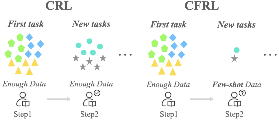
Figure 1: Difference between Continual Relation Learning (crl) and Continual Few-shot Relation Learning (cfrl). Except for the first task which has enough training data, the subsequent new tasks are all few-shot in cfrl. In contrast, crl assumes enough training data for every task.

A potential solution is to formalize RE as Continual Relation Learning or crl (Wang et al., 2019). In crl, the model learns relational knowledge through a sequence of tasks, where the relation set changes dynamically from the current task to the next. The model is expected to perform well on both the novel and previous tasks, which is challenging due to the existence of Catastrophic Forgetting phenomenon (McCloskey and Cohen, 1989; French, 1999) in continual learning. In this phenomenon, the model forgets previous relational knowledge after learning new relational patterns.

Existing methods to address catastrophic forgetting in crl can be divided into three categories: (i) regularization-based methods, (ii) architecture-based methods, and (iii) memory-based methods. Recent work shows that memory-based methods which save several key examples from previous tasks to a memory and reuse them when learning new tasks are more effective in NLP (Wang et al., 2019; Sun et al., 2020). Successful memory-based crl methods include EAEMR (Wang et al., 2019), MLLRE (Obamuyide and Vlachos, 2019), EMAR (Han et al., 2020), and CML (Wu et al., 2021).

Despite their effectiveness, one major limitation of these methods is that they all assume plenty of training data for learning new relations (tasks), which is hard to satisfy in real scenario where continual learning is desirable, as acquiring large labeled datasets for every new relation is expensive and sometimes impractical for quick deployment (e.g., RE from news articles during the onset of an emerging event like Covid-19). In fact, one of the main objectives of continual learning is to quickly adapt to new environments or tasks by exploiting previously acquired knowledge, a hallmark of human intelligence Lopez-Paz and Ranzato (2017). If the new tasks are few-shot, the existing methods suffer from over-fitting as shown later in our experiments (section 4). Considering that humans can acquire new knowledge from a handful of examples, it is expected for the models to generalize well on the new tasks with few data. We regard this problem as Continual Few-shot Relation Learning or cfrl (Fig. 1). Indeed, in relation to cfrl, Zhang et al. (2021), Zhu et al. (2021) and Chen and Lee (2021) recently introduce methods for incremental few-shot learning in Computer Vision.

Based on the observation that the learning of emerging few-shot tasks may result in distorted feature distributions of new data which are incompatible with previous embedding space (Ren et al., 2020), this work introduces a novel model based on Embedding space Regularization and Data Augmentation (ERDA) for cfrl. In particular, we propose a multi-margin loss and a pairwise margin loss in addition to the cross-entropy loss to impose further relational constraints in the embedding space. We also introduce a novel contrastive loss to learn more effectively from the memory data. Our proposed data augmentation method selects relevant samples from unlabeled text to provide more relational knowledge for the few-shot tasks. The empirical results show that our method can significantly outperform previous state-of-the-art methods. In summary, our main contributions are:

• To the best of our knowledge, we are the first one to consider cfrl. We define the cfrl problem and construct a benchmark for the problem.

• We propose ERDA, a novel method for cfrl based on embedding space regularization and data augmentation.

• With extensive experiments, we demonstrate the effectiveness of our method compared to existing ones and analyse our results thoroughly.

2 Related Work

Conventional RE methods include supervised (Zelenko et al., 2002; Liu et al., 2013; Zeng et al., 2014; Miwa and Bansal, 2016), semi-supervised (Chen et al., 2006; Sun et al., 2011; Hu et al., 2020) and distantly supervised methods (Mintz et al., 2009; Yao et al., 2011; Zeng et al., 2015; Han et al., 2018a). These methods rely on a predefined relation set and have limitations in real scenario where novel relations are emerging. There have been some efforts which focus on relation learning without predefined types, including open RE (Shinyama and Sekine, 2006; Etzioni et al., 2008; Cui et al., 2018; Gao et al., 2020) and continual relation learning (Wang et al., 2019; Obamuyide and Vlachos, 2019; Han et al., 2020; Wu et al., 2021).

Continual Learning (CL) aims to learn knowledge from a sequence of tasks. The main problem CL attempts to address is catastrophic forgetting (McCloskey and Cohen, 1989), i.e., the model forgets previous knowledge after learning new tasks. Prior methods to alleviate this problem can be mainly divided into three categories. First, regularization-based methods impose constraints on the update of neural weights important to previous tasks to alleviate catastrophic forgetting (Li and Hoiem, 2017; Kirkpatrick et al., 2017; Zenke et al., 2017; Ritter et al., 2018). Second, architecture-based methods dynamically change model architectures to acquire new information while remembering previous knowledge (Chen et al., 2016; Rusu et al., 2016; Fernando et al., 2017; Mallya et al., 2018). Finally, memory-based methods maintain a memory to save key samples of previous tasks to prevent forgetting (Rebuffi et al., 2017; Lopez-Paz and Ranzato, 2017; Shin et al., 2017; Chaudhry et al., 2019). These methods mainly focus on learning a single type of tasks. More recently, researchers have considered lifelong language learning (Sun et al., 2020; Qin and Joty, 2022), where the model is expected to continually learn from different types of tasks.

Few-shot Learning (FSL) aims to solve tasks containing only a few labeled samples, which faces the issue of over-fitting. To address this, existing methods have explored three different directions: (i) data-based methods use prior knowledge to augment data to the few-shot set (Santoro et al., 2016; Benaim and Wolf, 2018; Gao et al., 2020); (ii) model-based methods reduce the hypothesis space using prior knowledge (Rezende et al., 2016; Triantafillou et al., 2017; Hu et al., 2018); and (iii) algorithm-based methods try to find a more suitable strategy to search for the best hypothesis in the whole hypothesis space (Hoffman et al., 2013; Ravi and Larochelle, 2017; Finn et al., 2017).

Summary. Existing work in crl which involves a sequence of tasks containing sufficient training data, mainly focuses on alleviating the catastrophic forgetting of previous relational knowledge when the model is trained on new tasks. The work in few-shot learning mostly leverages prior knowledge to address the over-fitting of novel few-shot tasks. In contrast to these lines of work, we aim to solve a more challenging yet more practical problem cfrl where the model needs to learn relational patterns from a sequence of few-shot tasks continually.

3 Methodology

In this section, we first formally define the cfrl problem. Then, we present our method for cfrl.

3.1 Problem Definition

cfrl involves learning from a sequence of tasks ${\mathbb{T}}=({\mathcal{T}}^{1},\ldots,{\mathcal{T}}^{n})$, where every task $\mathcal{T}^{k}$ has its own training set $D_{\text{train}}^{k}$, validation set $D_{\text{valid}}^{k}$, and test set $D_{\text{test}}^{k}$. Each dataset $D$ contains several samples $\{(x_{i},y_{i})\}_{i=1}^{|D|}$, whose labels $y_{i}$ belong to the relation set $R^{k}$ of task $\mathcal{T}^{k}$. In contrast to the previously addressed continual relation learning (crl), cfrl assumes that except for the first task which has enough data for training, the subsequent new tasks are all few-shot, meaning that they have only few labeled instances (see Fig. 1). For example, consider there are three relation learning tasks $\mathcal{T}^{1},\mathcal{T}^{2}$ and $\mathcal{T}^{3}$ with their corresponding relation sets $R^{1},R^{2}$, and $R^{3}$, each having $10$ relations. In cfrl, we assume the existing task $\mathcal{T}^{1}$ has enough training data (e.g., $100$ samples for every relation in $R^{1}$), while the new tasks $\mathcal{T}^{2}$ and $\mathcal{T}^{3}$ are few-shot with only few (e.g., $5$) samples for every relation in $R^{2}$ and $R^{3}$. Assuming that the relation number of each few-shot task is $N$ and the sample number of every relation is $K$, we call this setup $N$-way $K$-shot continual learning. The problem setup of cfrl is aligned with the real scenario, where we generally have sufficient data for an existing task, but only few labeled data as new tasks emerge.

The model in cfrl is expected to first learn $\mathcal{T}^{1}$ well, which has sufficient training data to obtain good ability to extract the relation information in the sentence. Then at time step $k$, the model will be trained on the training set $D_{\text{train}}^{k}$ of few-shot task $\mathcal{T}^{k}$. After learning $\mathcal{T}^{k}$, the model is expected to perform well on both $\mathcal{T}^{k}$ and the previous $k$$-$$1$ tasks, as the model will be evaluated on $\hat{D}_{\text{test}}^{k}=\cup_{i=1}^{k}D_{\text{test}}^{i}$ consisting of all known relations after learning $\mathcal{T}^{k}$, i.e., $\hat{R}^{k}=\cup_{i=1}^{k}R^{i}$. This requires the model to overcome the catastrophic forgetting of previous knowledge and to learn new knowledge well with very few labeled data.

To overcome the catastrophic forgetting problem, a memory $\mathcal{M}=\left\{\mathcal{M}^{1},\mathcal{M}^{2},...\right\}$, which stores some key samples of previous tasks is maintained during the learning. When the model is learning $\mathcal{T}^{k}$, it has access to the data saved in memory $\mathcal{M}^{1},...,\mathcal{M}^{k-1}$. As there is no limit on the number of tasks, the size of memory $\mathcal{M}^{k}$ is constrained to be small. Therefore, the model has to select only key samples from the training set $D_{\text{train}}^{k}$ to save them in $\mathcal{M}^{k}$. In our cfrl setting, only one sample per relation is allowed to be saved in the memory.

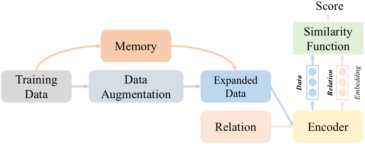
Figure 2: Our framework for cfrl. The Data Augmentation component is used only for few-shot tasks ($k>1$).

3.2 Overall Framework

Our framework for cfrl is shown in Fig. 2 and Alg. 1 describes the overall training process (see Appendix  A.1 for a block diagram). At time step $k$, given the training data $D_{\text{train}}^{k}$ for the task $\mathcal{T}^{k}$, depending on whether the task is a few-shot or not, the process has four or three working modules, respectively. The general learning process (section 3.3) has three steps that apply to all tasks. If the task is a few-shot task ($k>1$), we apply an additional step to create an augmented training set $\widetilde{D}_{\text{train}}^{k}$. For the initial task ($k=1$), we have $\widetilde{D}_{\text{train}}^{k}=D_{\text{train}}^{k}$.

For any task $\mathcal{T}^{k}$, we use a siamese model to encode every new relation $r_{i}\in R^{k}$ into $\mathbf{r}_{i}\in\operatorname{\rm I\!R}^{d}$ as well as the sentences, and train the model on $\widetilde{D}_{\text{train}}^{k}$ to acquire relation information of the new data (section 3.3.2). To overcome forgetting, we select the most informative sample for each relation $r_{i}\in R^{k}$ from $D_{\text{train}}^{k}$ and update the memory $\hat{\mathcal{M}^{k}}$ (section 3.3.3). Finally, we combine $\widetilde{D}_{\text{train}}^{k}$ and $\hat{\mathcal{M}^{k}}$ as the training data for learning new relational patterns and remembering previous knowledge (section 3.3.4). We also simultaneously update the representation of all relations in $\hat{R}^{k}$, which involves making a forward pass through the current model. The learning and updating are done iteratively for convergence.

For data augmentation in few-shot tasks (section 3.4), we select reliable samples with high relational similarity score from an unlabelled Wikipedia corpus using a fine-tuned BERT (Devlin et al., 2019), which serves as the relational similarity model $\mathcal{S}_{\pi}$. In the interests of coherence, we first present the general learning method followed by the augmentation process for few-shot learning.

Algorithm 1 Training process at time step $k$

1:the training set $D_{\text{train}}^{k}$ and the relation set $R^{k}$ of the current task $\mathcal{T}^{k}$, the current memory $\hat{\mathcal{M}}^{k-1}$ and the known relation set $\hat{R}^{k-1}$, the model $\theta$, the similarity model $\mathcal{S}_{\pi}$, and the unlabeled text corpus $\mathcal{C}$.

2:if $k==1$ then $\triangleright$ initial task

3:     $\widetilde{D}_{\text{train}}^{k}=D_{\text{train}}^{k}$

4:else$\triangleright$ few-shot task

5:     Select similar samples from $\mathcal{C}$ using $\mathcal{S}_{\pi}$ for every sample in $D_{\text{train}}^{k}$ and store them in $A$

6:     $\widetilde{D}_{\text{train}}^{k}=A\cup D_{\text{train}}^{k}$

7:end if

8:Initialize $\mathbf{r}_{i}$ for every relation $r_{i}\in R^{k}$

9:for $i=1,\ldots,{iter}_{1}$ do

10:     Update $\theta$ with $\mathcal{L}_{\text{new}}$ on $\widetilde{D}_{\text{train}}^{k}$ $\triangleright$ Train on new task

11:end for

12:Select key samples from $D_{\text{train}}^{k}$ for every relation $r_{i}\in R^{k}$ to save in $\mathcal{M}^{k}$

13:$\hat{R}^{k}=\hat{R}^{k-1}\cup R^{k}$

14:$\hat{\mathcal{M}^{k}}=\hat{\mathcal{M}}^{k-1}\cup\mathcal{M}^{k}$ $\triangleright$ Update memory

15:$\widetilde{H}^{k}=\widetilde{D}_{\text{train}}^{k}\cup\hat{\mathcal{M}^{k}}$ $\triangleright$ Combine two data sources

16:for $i=1,\ldots,{iter}_{2}$ do

17:     Update $\theta$ with $\mathcal{L}_{\text{mem}}$ on $\widetilde{H}^{k}$

18:     Update $\mathbf{r}_{i}$ for every relation $r_{i}\in\hat{R}^{k}$

19:end for

3.3 General Learning Process

We first introduce the encoder network as it is the basic component of the whole framework.

3.3.1 The Encoder Network

The siamese encoder ($f_{\theta}$) aims at extracting generic and relation related features from the input. The input can be a labeled sentence or the name of a relation. We adopt two kinds of encoders:

$\bullet$ Bi-LSTM

To have a fair comparison with previous work, we use the same architecture as Han et al. (2020). It takes GloVe embeddings (Pennington et al., 2014) of the words in a given input and produces a vector representation through a Bi-LSTM (Hochreiter and Schmidhuber, 1997).

$\bullet$ BERT

We adopt $\rm{BERT_{base}}$ which has 12 layers and 110M parameters. As the new tasks are few-shot, we only fine-tune the 12-th encoding layer and the extra linear layer. We include special tokens around the entities (‘#’ for the head entity and ‘@’ for the tail entity) in a given labeled sentence to improve the encoder’s understanding of relation information. We use the [cls] token features as the representation of the input sequence.

3.3.2 Learning with New Data

At time step $k$, to have a good understanding of the new relations, we fine-tune the model on the expanded dataset $\widetilde{D}_{\text{train}}^{k}$. The model $f_{\theta}$ first encodes the name of each new relation $r_{j}\in R^{k}$ into its representation $\mathbf{r}_{j}\in\operatorname{\rm I\!R}^{d}$ by making a forward pass. Then, we optimize the parameters ($\theta$) by minimizing a loss $\mathcal{L}_{\text{new}}$ that consists of a cross entropy loss, a multi-margin loss and a pairwise margin loss.

The cross entropy loss $\mathcal{L}_{\text{ce}}$ is used for relation classification as follows.

$$\sum_{(x_{i},y_{i})\in\widetilde{D}_{\text{train}}^{k}}\sum_{j=1}^{|\hat{R}^{k}|}\delta_{y_{i},r_{j}}\times\log\frac{\exp(g(f_{\theta}(x_{i}),\mathbf{r}_{j}))}{\sum_{l=1}^{|\hat{R}^{k}|}\exp(g(f_{\theta}(x_{i}),\mathbf{r}_{l}))}$$ (1)

where $\hat{R}^{k}$ is the set of all known relations at step $k$, $g(,)$ is a function used to measure similarity between two vectors (e.g., cosine similarity or L2 distance), and $\delta_{a,b}$ is the Kronecker delta function– $\delta_{a,b}=1$ if $a$ equals $b$, otherwise $\delta_{a,b}=0$.

In inference, we choose the relation label that has the highest similarity with the input sentence (Eq. 8). To ensure that an example has the highest similarity with the true relation, we additionally design two margin-based losses, which increase the score between an example and the true label while decreasing the scores for the wrong labels. The first one is a multi-margin loss defined as:

$$\mathcal{L}_{\text{mm}} =\sum_{(x_{i},y_{i})\in\widetilde{D}_{\text{train}}^{k}}\sum_{j=1,j\neq t_{i}}^{|\hat{R}^{k}|}\max\Big{(}0,$$ (2)

$$m_{1}-g(f_{\theta}(x_{i}),\mathbf{r}_{t_{i}})+g(f_{\theta}(x_{i}),\mathbf{r}_{j})\Big{)}$$

where $t_{i}$ is the correct relation index in $\hat{R}^{k}$ satisfying $r_{t_{i}}=y_{i}$ and $m_{1}$ is a margin value. The $\mathcal{L}_{\text{mm}}$ loss attempts to ensure intra-class compactness while increasing inter-class distances. The second one is a pairwise margin loss $\mathcal{L}_{\text{pm}}$:

$$\sum_{~{}~{}(x_{i},y_{i})\in\widetilde{D}_{\text{train}}^{k}}\max\Big{(}0,m_{2}-g(f_{\theta}(x_{i}),\mathbf{r}_{t_{i}})+g(f_{\theta}(x_{i}),\mathbf{r}_{s_{i}})\Big{)}$$ (3)

where $m_{2}$ is the margin for $\mathcal{L}_{\text{pm}}$ and $s_{i}=\mathop{\arg\max}_{s}g(f_{\theta}(x_{i}),\mathbf{r}_{s})$ s.t. $s\neq t_{i}$, the closest wrong label. The $\mathcal{L}_{\text{pm}}$ loss penalizes the cases where the similarity score of the closest wrong label is higher than the score of the correct label (Yang et al., 2018). Both $\mathcal{L}_{\text{mm}}$ and $\mathcal{L}_{\text{pm}}$ improve the discriminative ability of the model (section 4.4).

The total loss for learning on $\mathcal{T}^{k}$ is defined as:

$$\mathcal{L}_{new}=\lambda_{\text{ce}}\mathcal{L}_{\text{ce}}+\lambda_{\text{mm}}\mathcal{L}_{\text{mm}}+\lambda_{\text{pm}}\mathcal{L}_{\text{pm}}\normalsize$$ (4)

where $\lambda_{\text{ce}}$, $\lambda_{\text{mm}}$ and $\lambda_{\text{pm}}$ are the relative weights of the component losses, respectively.

3.3.3 Selecting Samples for Memory

After training the model $f_{\theta}$ with Eq. (4), we use it to select one sample per new relation. Specifically, for every new relation $r_{j}\in R^{k}$, we obtain the centroid feature $\mathbf{c}_{j}$ by averaging the embeddings of all samples labeled as $r_{j}$ in $D_{\text{train}}^{k}$ as follows.

$$\mathbf{c}_{j}=\frac{1}{|D_{r_{j}}^{k}|}\sum_{(x_{i},y_{i})\in D_{r_{j}}^{k}}f_{\theta}(x_{i})\normalsize$$ (5)

where $D_{r_{j}}^{k}=\{(x_{i},y_{i})|(x_{i},y_{i})\in D_{\text{train}}^{k},y_{i}=r_{j}\}$. Then we select the instance closest to $\mathbf{c}_{j}$ from $D_{r_{j}}^{k}$ as the most informative sample and save it in memory $\mathcal{M}^{k}$. Note that the selection is done from $D_{\text{train}}^{k}$, not from the expanded set $\widetilde{D}_{\text{train}}^{k}$.

3.3.4 Alleviating Forgetting through Memory

As the learning of new relational patterns may cause catastrophic forgetting of previous knowledge (see baselines in section 4), our model needs to learn from the memory data to alleviate forgetting. We combine the expanded set $\widetilde{D}_{\text{train}}^{k}$ and the whole memory data $\hat{\mathcal{M}^{k}}=\cup_{j=1}^{k}\mathcal{M}^{j}$ into $\widetilde{H}^{k}$ to allow the model to learn new relational knowledge and consolidate previous knowledge. However, the memory data is limited containing only one sample per relation. To learn effectively from such limited data, we design a novel method to generate a hard negative sample set ${P}_{i}$ for every sample in $\hat{\mathcal{M}^{k}}$.

The negative samples are generated on the fly. After sampling a mini-batch $B_{t}$ from $\widetilde{H}^{k}$, we consider all memory data in $B_{t}$ as $M_{B_{t}}$. For every sample $(\hat{x}_{i},\hat{y}_{i})$ in $M_{B_{t}}$, we replace its head entity $e_{i}^{h}$ or tail entity $e_{i}^{t}$ with the corresponding entity of a randomly selected sample in the same batch $B_{t}$ to get the hard negative sample set ${P}_{i}=\{(\hat{x}_{j}^{P_{i}},\hat{y}_{i})\}_{j=1}^{|{P}_{i}|}$. Then $(\hat{x}_{i},\hat{y}_{i})$ and ${P}_{i}$ are used to calculate a margin-based contrastive loss $\mathcal{L}_{\text{con}}$ as follows.

$$\mathcal{L}_{\text{con}}=\sum_{(\hat{x}_{i},\hat{y}_{i})\in M_{B_{t}}} \max\Big{(}0,m_{3}-g(f_{\theta}(\hat{x}_{i}),\mathbf{r}_{\hat{t}_{i}})+$$ (6)

$$\sum_{(\hat{x}_{j}^{P_{i}},\hat{y}_{i})\in{P}_{i}}g(f_{\theta}(\hat{x}_{j}^{P_{i}}),\mathbf{r}_{\hat{t}_{i}})\Big{)}$$

where $\hat{t}_{i}$ is the relation index satisfying $r_{\hat{t}_{i}}=\hat{y}_{i}$ and $m_{3}$ is the margin value for $\mathcal{L}_{\text{con}}$. This loss forces the model to distinguish the valid relations from the hard negatives so that the model learns more precise and fine-grained relational knowledge. In addition, we also use the three losses $\mathcal{L}_{\text{ce}}$ and $\mathcal{L}_{\text{mm}}$ and $\mathcal{L}_{\text{pm}}$ defined in Section 3.3.2 to update $\theta$ on $B_{t}$. The total loss on the memory data is:

$$\mathcal{L}_{\text{mem}} =\lambda_{\text{ce}}\mathcal{L}_{\text{ce}}+\lambda_{\text{mm}}\mathcal{L}_{\text{mm}}+\lambda_{\text{pm}}\mathcal{L}_{\text{pm}}+\lambda_{\text{con}}\mathcal{L}_{\text{con}}$$ (7)

where $\lambda_{\text{ce}}$, $\lambda_{\text{mm}}$, $\lambda_{\text{pm}}$ and $\lambda_{\text{con}}$ are the relative weights of the corresponding losses.

Updating Relation Embeddings

After training the model on $\widetilde{H}^{k}$ for few steps, we use the memory $\hat{\mathcal{M}^{k}}$ to update the relation embedding $\mathbf{r}_{i}$ of all known relations. For a relation $r_{i}\in\hat{R}^{k}$, we average the embeddings (obtained by making a forward pass through $f_{\theta}$) of the relation name and memory data to obtain its updated representation $\mathbf{r}_{i}$. The training of $\theta$ and updating of $\mathbf{r}_{i}$ is done iteratively to grasp new relational patterns while alleviating the catastrophic forgetting of previous knowledge.

3.3.5 Inference

For a given input $x_{i}$ in $\hat{D}_{\text{test}}^{k}$, we calculate the similarity between $x_{i}$ and all known relations, and pick the one with the highest similarity score:

$$y_{i}^{*}=\mathop{\arg\max}\limits_{r\in\hat{R}^{k}}g(f_{\theta}(x_{i}),\mathbf{r})\normalsize$$ (8)

3.4 Data Augmentation for Few-shot Tasks

For each few-shot task $\mathcal{T}^{k}$, we aim to get more data by selecting reliable samples from an unlabeled corpus $\mathcal{C}$ with tagged entities before the general learning process (section 3.3) begins. We achieve this using a relational similarity model $\mathcal{S}_{\pi}$ and sentences from Wikipedia as $\mathcal{C}$. The model $\mathcal{S}_{\pi}$ (described later) takes a sentence as input and produces a normalized vector representation. The cosine similarity between two vectors is used to measure the relational similarity between the two corresponding sentences. A higher similarity means the two sentences are more likely to have the same relation label. We propose two novel selection methods, which are complementary to each other.

(a) Augmentation via Entity Matching

For each instance $(x_{i},y_{i})$ in $D_{\text{train}}^{k}$, we extract its entity pair $(e_{i}^{h},e_{i}^{t})$ with $e_{i}^{h}$ being the head entity and $e_{i}^{t}$ being the tail entity. As sentences with the same entity pair are more likely to express the same relation, we first collect a candidate set $\mathcal{Q}=\left\{\widetilde{x}_{j}\right\}_{j=1}^{|\mathcal{Q}|}$ from $\mathcal{C}$, where $\widetilde{x}_{j}$ shares the same entity pair $(e_{i}^{h},e_{i}^{t})$ with $x_{i}$. If $\mathcal{Q}$ is a non-empty set, we pair all $\widetilde{x}_{j}$ in $\mathcal{Q}$ with $x_{i}$, and denote each pair as $\langle\widetilde{x}_{j},x_{i}\rangle$. Then we use $\mathcal{S}_{\pi}$ to obtain a similarity score $\mathrm{s}_{j}$ for $\langle\widetilde{x}_{j},x_{i}\rangle$. After getting scores for all pairs, we pick the instances $\widetilde{x}_{j}$ with similarity score $\mathrm{s}_{j}$ higher than a predefined threshold $\alpha$ as new samples and label them with relation $y_{i}$. The selected instances are then augmented to $D_{\text{train}}^{k}$ as additional data.

(b) Augmentation via Similarity Search

The hard entity matching could be too restrictive at times. For example, even though the sentences “Harry Potter is written by Joanne Rowling” and “Charles Dickens is the author of A Tale of Two Cities” share the same relation author, hard matching fails to find any relevance. Therefore, in cases when entity matching returns an empty $\mathcal{Q}$, we resort to similarity search using Faiss (Johnson et al., 2017). Given a query vector $\mathbf{q}_{i}$, it can efficiently search for vectors $\{\mathbf{v}_{j}\}_{j=1}^{K}$ with the top-$K$ highest similarity scores in a large vector set ${\mathcal{V}}$. In our case, $\mathbf{q}_{i}$ is the representation of $x_{i}$ and $\mathcal{V}$ contains the representations of the sentences in $\mathcal{C}$. We use $\mathcal{S}_{\pi}$ to obtain these representations; the difference is that $\mathcal{V}$ is pre-computed while $\mathbf{q}_{i}$ is obtained during training. We labeled the top-$K$ most similar instances with $y_{i}$ and augment them to $D_{\text{train}}^{k}$.

Similarity Model

To train $\mathcal{S}_{\pi}$, inspired by Soares et al. (2019), we adopt a contrastive learning method to fine-tune a $\rm{BERT_{base}}$ model on $\mathcal{C}$, whose sentences are already tagged with entities. Based on the observation that sentences with the same entity pair are more likely to encode the same relation, we use sentence pairs containing the same entities in $\mathcal{C}$ as positive samples. For negatives, instead of using all sentence pairs containing different entities, we select pairs sharing only one entity as hard negatives (i.e., pair $(x_{i},x_{j})$ where $e_{i}^{h}=e_{j}^{h}$ and $e_{i}^{t}\neq e_{j}^{t}$ or $e_{i}^{t}=e_{j}^{t}$ and $e_{i}^{h}\neq e_{j}^{h}$ ). We randomly sample the same number of negative samples as the positive ones to balance the training.

For an input pair $(x_{i},x_{j})$, we compute the similarity score based on the following formula.

$$\sigma(x_{i},x_{j})=\frac{1}{1+\exp(-\mathcal{S}_{\pi}(x_{i})^{T}\mathcal{S}_{\pi}(x_{j}))}\normalsize$$ (9)

where $\mathcal{S}_{\pi}(x)$ is the normalized representation of $x$ obtained from the final layer of BERT. Then we optimize the parameters $\pi$ of $\mathcal{S}_{\pi}$ by minimizing a binary cross entropy loss $\mathcal{L}_{\text{pretrain}}$ as follows.

$$-\sum_{(x_{i},x_{j})\in\mathcal{C}_{p}}\log\sigma(x_{i},x_{j})-\sum_{(x_{i}^{\prime},x_{j}^{\prime})\in\mathcal{C}_{n}}\log(1-\sigma(x_{i}^{\prime},x_{j}^{\prime}))$$ (10)

where $\mathcal{C}_{p}$ is a positive batch and $\mathcal{C}_{n}$ is a negative batch. This objective tries to ensure that sentence pairs with the same entity pairs have higher cosine similarity than those with different entities.

4 Experiment

We define the benchmark and evaluation metric for cfrl before presenting our experimental results.

4.1 Benchmark and Evaluation Metric

Benchmark   As the benchmark for cfrl needs to have sufficient relations as well as data and be suitable for few-shot learning, we create the cfrl benchmark based on FewRel (Han et al., 2018b). FewRel is a large-scale dataset for few-shot RE, which contains $80$ relations with hundreds of samples per relation. We randomly split the $80$ relations into $8$ tasks, where each task contains $10$ relations (10-way). To have enough data for the first task $\mathcal{T}^{1}$, we sample $100$ samples per relation. All the subsequent tasks $\mathcal{T}^{2},...,\mathcal{T}^{8}$ are few-shot; for each relation, we conduct 2-shot, 5-shot and 10-shot experiments to verify the effectiveness of our method.

In addition, to demonstrate the generalizability of our method, we also create a cfrl benchmark based on the TACRED dataset (Zhang et al., 2017) which contains only $42$ relations. We filter out the special relation “n/a” (not available) and split the remaining $41$ relations into $8$ tasks. Except for the first task that contains $6$ relations, all other tasks have $5$ relations (5-way). Similar to FewRel, we randomly sample $100$ examples per relation in $\mathcal{T}^{1}$ and conduct 5-shot and 10-shot experiments.

Metric

At time step $k$, we evaluate the model performance through relation classification accuracy on the test sets $\hat{D}_{\text{test}}^{k}=\cup_{i=1}^{k}D_{\text{test}}^{i}$ of all seen tasks $\{\mathcal{T}^{i}\}_{i=1}^{k}$. This metric reflects whether the model can alleviate catastrophic forgetting while acquiring novel knowledge well with very few data. Since the model performance might be influenced by task sequences and few-shot training samples, we run every experiment $6$ times each time with a different random seed to ensure a random task order and model initialization, and report the average accuracy along with variance. We perform paired t-test for statistical significance.

4.2 Model Settings & Baselines

The model settings are shown in Appendix A.2. We compare our approach with the following baselines:

• SeqRun fine-tunes the model only on the training data of the new tasks without using any memory data. It may face serious catastrophic forgetting and serves as a lower bound.

• Joint Training stores all previous samples in the memory and trains the model on all data for each new task. It serves as an upper bound in crl.

• EMR (Wang et al., 2019) maintains a memory for storing selected samples from previous tasks. When training on a novel task, EMR combines the new training data and memory data.

• EMAR (Han et al., 2020) is the state-of-the-art on crl, which adopts memory activation and reconsolidation to alleviate catastrophic forgetting.

• IDLVQ-C (Chen and Lee, 2021) introduces quantized reference vectors to represent previous knowledge and mitigates catastrophic forgetting by imposing constraints on the quantized vectors and embedded space. It was originally proposed for image classification with state-of-the-art results in incremental few-shot learning.

Method	Task index
	1	2	3	4	5	6	7	8
SeqRun	$92.78$	$52.11$	$30.08$	$24.33$	$19.83$	$16.90$	$14.36$	$12.34$
Joint Train	$\mathbf{92.78}$	$76.29$	$69.39$	$64.75$	$60.45$	$\mathbf{57.64}$	$52.80$	$50.03$
EMR	$92.78$	$69.14$	$56.24$	$50.03$	$46.50$	$43.21$	$39.88$	$37.51$
EMAR	$85.20$	$62.02$	$52.45$	$48.95$	$46.77$	$44.33$	$40.75$	$39.04$
IDLVQ-C	$92.23$	$69.15$	$57.42$	$51.66$	$49.31$	$46.24$	$42.25$	$40.56$
ERDA	$92.57$	$\mathbf{79.17}$	$\mathbf{70.43}$	$\mathbf{65.01}$	$\mathbf{61.06}$	$\mathbf{57.54}$	$\mathbf{54.88}$	$\mathbf{53.23}$

Table 1: Accuracy ($\%$) of different methods at every time step on FewRel benchmark for $10$-way $5$-shot cfrl. ERDA is significantly better than IDLVQ-C with $p$-value $<0.001$.

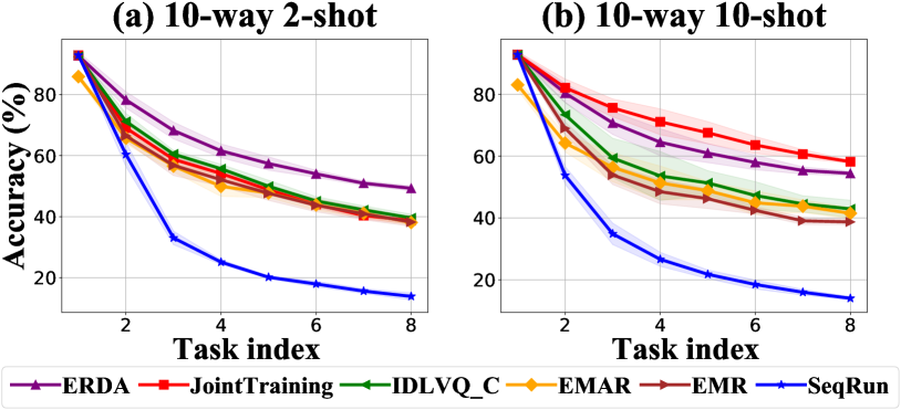
Figure 3: Comparison results at each time step on FewRel benchmark for $10$-way $2$-shot and $10$-shot settings. For both settings, ERDA is significantly better than IDLVQ-C with $p$-value $<0.001$. The variance is reported as light color region.

4.3 Main Results

We compare the performance of different methods using the same setting as EMAR Han et al. (2020), which uses a Bi-LSTM encoder. We also report the results with a BERT encoder.

FewRel Benchmark

We report our results on 10-way 5-shot in Table 1, while Fig. 3 shows the results on the 10-way 2-shot and 10-way 10-shot settings. From the results, we can observe that:

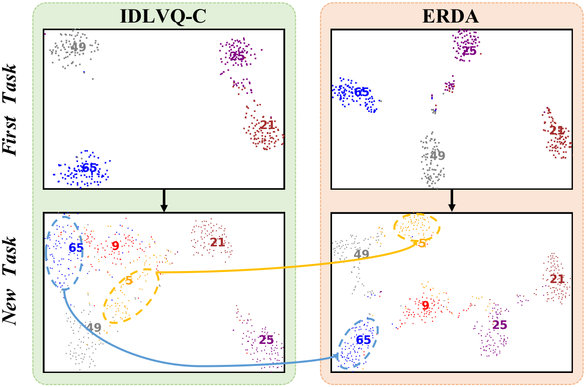
Figure 4: t-SNE visualization of IDLVQ-C and ERDA at two stages. Colors represent different relation classes with numbers being the relation indices. The initial embeddings of four base classes after learning the first task are shown in the upper row. As the data for the first task is sufficient, both methods can obtain separable embedding space. The lower row shows the embeddings of four base classes and two novel classes (Id 5 and 9) after learning a new few-shot task. Compared with IDLVQ-C, ERDA shows better intra-class compactness (circled regions) and larger inter-class distances (see the distances between 5 and 9, and 9 and 65).

$\bullet~{}$ Our proposed ERDA outperforms previous baselines in all cfrl settings, which demonstrates the superiority of our method. Simply fine-tuning the model with new few-shot examples leads to rapid drops in accuracy due to severe over-fitting and catastrophic forgetting. Although EMR and EMAR adopt a memory module to alleviate forgetting, their performance still decreases quickly as they require plenty of training data for learning a new task. Compared with EMR and EMAR, IDLVQ-C is slightly better as it introduces quantized vectors that can better represent the embedding space of few-shot tasks. However, IDLVQ-C does not necessarily push the samples from different relations to be far apart in the embedding space and the updating method for the reference vectors may not be optimal. ERDA outperforms IDLVQ-C by a large margin through embedding space regularization and self-supervised data augmentation. To verify this, we show the embedding space of IDLVQ-C and ERDA using t-SNE (Van der Maaten and Hinton, 2008). We randomly choose four classes from the first task of FewRel and two classes from the new task, and visualize the test data of these classes in Fig. 4. As can be seen, the embedding space obtained by ERDA shows better intra-class compactness and larger inter-class distances.

$\bullet~{}$ Unlike crl, joint training does not always serve as an upper bound in cfrl due to the extremely imbalanced data distribution. Benefiting from the ability to learn feature distribution with very few data, both ERDA and IDLVQ-C perform better than joint training in the 2-shot setting. However, as the number of few-shot samples increases, the performance of IDLVQ-C falls far behind joint training, while ERDA still performs better. In the 5-shot setting, ERDA could achieve better results than joint training which verifies the effectiveness of self-supervised data augmentation (more on this in section 4.4). Although ERDA performs worse than joint training in the 10-shot setting, its results are still much better than other baselines.

$\bullet~{}$ After learning all few-shot tasks, ERDA outperforms IDLVQ-C by 9.69$\bm{\%}$, 12.67$\bm{\%}$ and 11.49$\bm{\%}$ in the 2-shot, 5-shot and 10-shot settings, respectively. Moreover, the relative gain of ERDA keeps growing with the increasing number of new few-shot tasks. This demonstrates the ability of our method in handling a longer sequence of cfrl tasks.

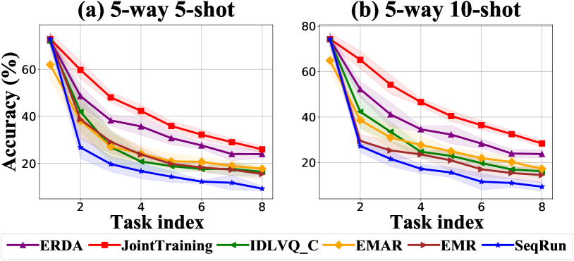
Figure 5: Comparison results at every time step on TACRED benchmark for $5$-way $5$-shot and $10$-shot settings. ERDA is significantly better than IDLVQ-C with $p$-value $<0.001$ for both settings. The variance is reported as light color region.

TACRED Benchmark

Fig. 5 shows the 5-way 5-shot and 5-way 10-shot results on TACRED. We can see that here also ERDA outperforms all other methods by a large margin which verifies the strong generalization ability of our proposed method.

Results with BERT

We show the results with $\rm{BERT_{base}}$ of different methods on FewRel in Fig. 6 for 10-way 2-shot and 10-shot and Table 4 for 10-way 5-shot (in Appendix). The results of on TACRED benchmark are shown in Fig. 7 for 5-way 5-shot and 10-shot. From the results, we can observe that ERDA outperforms previous baselines in all cfrl settings with a BERT encoder.

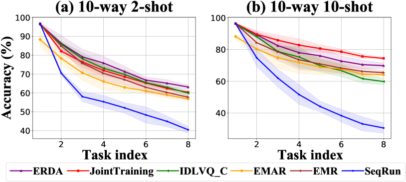
Figure 6: Comparison results of different methods with a BERT encoder on FewRel benchmark for $10$-way $2$-shot and $10$-shot settings. ERDA is significantly better than IDLVQ-C with $p$-value $=0.005$ for $2$-shot setting and is significantly better than EMR with $p$-value $=0.002$ for $10$-shot setting.

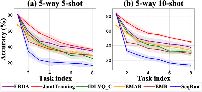
Figure 7: Results of different methods with a BERT encoder on TACRED benchmark for $5$-way $5$-shot and $10$-shot settings. ERDA is significantly better than EMR with $p$-value $=0.004$ for $5$-shot setting and is significantly better than EMAR with $p$-value $=0.02$ for $10$-shot setting.

4.4 Ablation Study

$\lambda_{con}$	0	0.01	0.02	0.05	0.1	0.2	0.5	1.0
Accuracy ($\%$)	$51.95_{\pm 1.15}$	$52.66_{\pm 1.23}$	$\mathbf{53.38}_{\pm 0.63}$	$53.10_{\pm 0.69}$	$53.23_{\pm 1.49}$	$52.99_{\pm 0.79}$	$52.13_{\pm 1.50}$	$52.27_{\pm 1.07}$

Table 2: Accuracy ($\%$) after learning all tasks with different $\lambda_{con}$ on FewRel benchmark ($10$-way $5$-shot).

We conduct several ablations to analyze the contribution of different components of ERDA on the FewRel 10-way 5-shot setting. In particular, we investigate seven other variants of ERDA by removing one component at a time: (a) the multi-margin loss $\mathcal{L}_{\text{mm}}$, (b) the pairwise margin loss $\mathcal{L}_{\text{pm}}$, (c) the margin-based contrastive loss $\mathcal{L}_{\text{con}}$, (d) the whole 2-stage data augmentation module, (e) the entity matching method of augmentation, (f) the similarity search method of augmentation, and (g) memory.

From the results in Table 3, we can observe that all components improve the performance of our model. Specifically, $\mathcal{L}_{\text{mm}}$ yields about 1.51$\%$ performance boost as it brings samples of the same relation closer to each other while enforcing larger distances among different relation distributions. The $\mathcal{L}_{\text{pm}}$ improves the accuracy by 3.18$\%$, which demonstrates the effect of contrasting with the nearest wrong label. The adoption of $\mathcal{L}_{\text{con}}$ leads to 1.28$\%$ improvement, which shows that generating hard negative samples for memory data can help to better remember previous relational knowledge. To better investigate the influence of $\mathcal{L}_{con}$, we conduct experiments with different $\lambda_{con}$ and show the results in Table 2. We can see that the model achieves the best accuracy of 53.38 with $\lambda_{con}=0.02$ while the accuracy is only 52.13 with $\lambda_{con}=0.5$. In addition, the performance of the variant without $\mathcal{L}_{con}$ is worse than the performance of all other variants, which demonstrates the effectiveness of $\mathcal{L}_{con}$.

The data augmentation module improves the performance by 1.72$\%$ as it can extract informative samples from unlabeled text which provide more relational knowledge for few-shot tasks. The results of variants without entity matching or similarity search verify that the two data augmentation methods are generally complementary to each other.

One could argue that the data augmentation module increases the complexity of ERDA compared to other models. However, astute readers can find that even without data augmentation, ERDA  outperforms IDLVQ-C significantly for all tasks (compare ‘ERDA w.o. DA’ with the baselines in Table 1).

ERDA’s Performance under crl

Although ERDA is designed for cfrl, we also evaluate the embedding space regularization (‘ERDA w.o. DA’) in the crl setting. We sample 100 examples per relation for every task in FewRel and compare our method with the state-of-the-art method EMAR. The results are shown in Fig. 8. We can see that ERDA outperforms EMAR in all tasks by 1.25 - 4.95$\%$ proving that the embedding regularization can be a general method for crl.

Method	Task index
	1	2	3	4	5	6	7	8
ERDA	$\mathbf{92.57}$	$\mathbf{79.17}$	$\mathbf{70.43}$	$\mathbf{65.01}$	$\mathbf{61.06}$	$\mathbf{57.54}$	$\mathbf{54.88}$	$\mathbf{53.23}$
w.o. $\mathcal{L}_{\text{mm}}$	$91.67$	$78.38$	$70.21$	$63.77$	$60.23$	$56.32$	$53.45$	$51.72$
w.o. $\mathcal{L}_{\text{pm}}$	$91.37$	$75.80$	$67.11$	$61.13$	$57.14$	$54.04$	$51.59$	$50.05$
w.o. $\mathcal{L}_{\text{con}}$	$91.63$	$79.05$	$69.28$	$63.86$	$59.66$	$56.68$	$54.12$	$51.95$
w.o. DA	$92.57$	$77.84$	$69.76$	$63.74$	$58.31$	$56.12$	$53.21$	$51.51$
w.o. EM	$92.57$	$78.33$	$70.17$	$64.18$	$59.63$	$57.10$	$54.18$	$52.39$
w.o. SS	$92.57$	$78.56$	$69.94$	$63.98$	$59.85$	$56.92$	$53.75$	$52.27$
w.o. M	$91.95$	$77.59$	$66.47$	$57.08$	$51.08$	$47.36$	$43.88$	$40.32$

Table 3: Ablations on FewRel benchmark ($10$-way $5$-shot). The variance over 6 runs is reported in Table 7 in Appendix. We show the analysis of ‘w.o. M’ in Appendix  A.4.

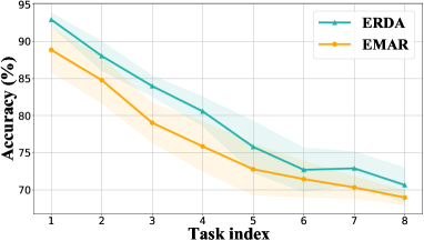
Figure 8: Relation extraction results for ERDA (our) and EMAR (Han et al., 2020) on the FewRel benchmark under the crl setting. We randomly split the 80 relations into 8 tasks, where each task contains 10 relations. And we sample 100 examples per relation. From this figure, we can observe that ERDA outperforms EMAR in all crl tasks.

5 Conclusion

We have introduced continual few-shot relation learning (cfrl), a challenging yet practical problem where the model needs to learn new relational knowledge with very few labeled data continually. We have proposed a novel method, named ERDA, to alleviate the over-fitting and catastrophic forgetting problems which are the core issues in cfrl. ERDA imposes relational constraints in the embedding space with innovative losses and adds extra informative data for few-shot tasks in a self-supervised manner to better grasp novel relational patterns and remember previous knowledge. Extensive experimental results and analysis show that ERDA significantly outperforms previous methods in all cfrl settings investigated in this work. In the future, we would like to investigate ways to combine meta-learning with cfrl.

Appendix A Appendix

A.1 Block Diagram of ERDA Training

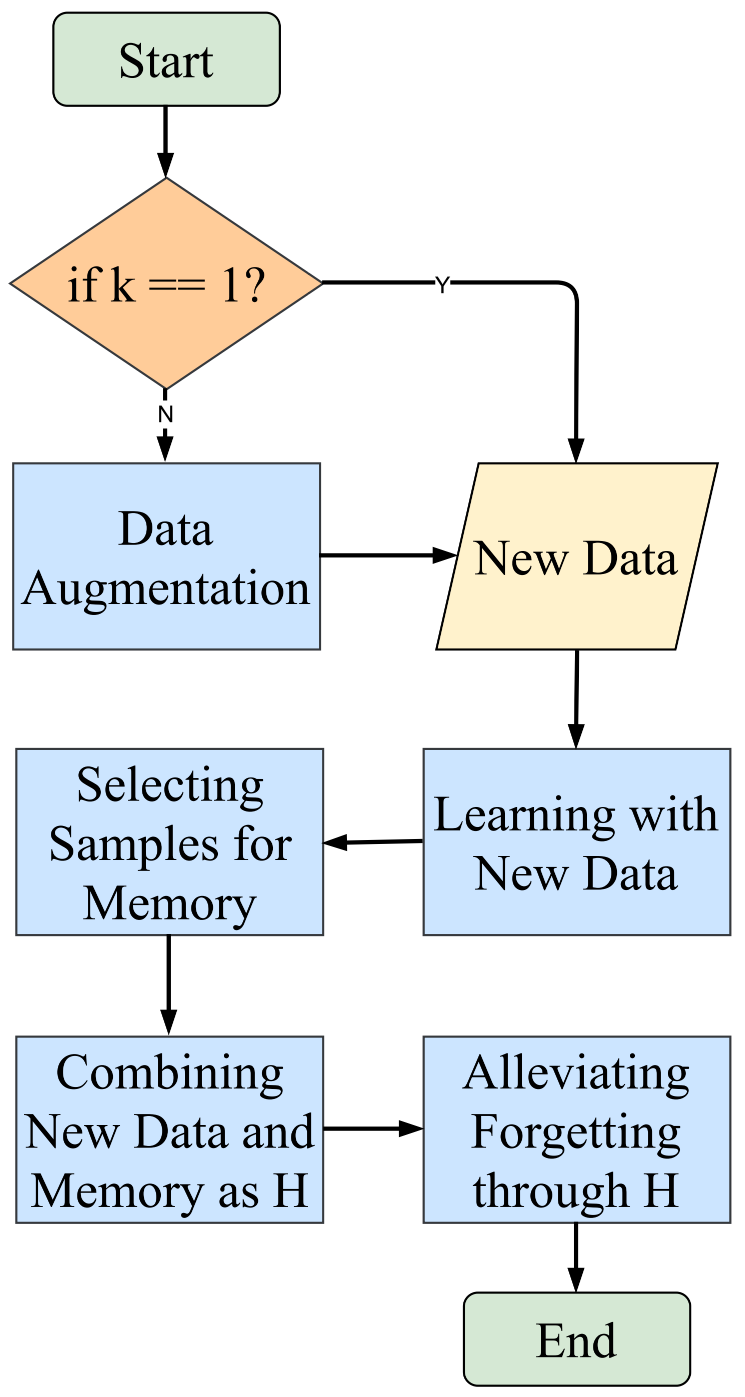
Figure 9: The block diagram of ERDA’s training at time step $k$.

A.2 Hyperparameter Search

We follow the settings in Han et al. (2020) for the Bi-LSTM encoder to have a fair comparison. For data augmentation, we set the threshold $\alpha=0.65$ and the number of samples selected by Faiss ($K$) as 1. We adopt $0.2,0.2$ and $0.01$ for the three margin values $m_{1},m_{2}$ and $m_{3}$, respectively. The loss weights $\lambda_{\text{ce}},\lambda_{\text{mm}},\lambda_{\text{pm}}$ and $\lambda_{\text{con}}$ are set to 1.0, 1.0, 1.0 and 0.1, respectively. In Alg. 1, we set $1$ for ${iter}_{1}$ and $2$ for ${iter}_{2}$. Hyperparameter search is done on the validation sets. We follow EMAR (Han et al., 2020) and use a grid search to select the hyperparameters. Specifically, the search spaces are:

• Search range for $\alpha$ is $\left[0.3,0.8\right]$ with a step size of $0.05$.

• Search range for $K$ is $\left[1,3\right]$ with a step size of $1$.

• Search range for $m_{1}$ and $m_{2}$ is $\left[0.1,0.3\right]$ with a step size of $0.1$.

• Search range for $m_{3}$ is $\left[0.01,0.03\right]$ with a step size of $0.01$.

• Search range for ${iter}_{2}$ in Alg. 1 is $\left[1,3\right]$ with a step size of $1$.

Method	Task index
	1	2	3	4	5	6	7	8
SeqRun	$96.35_{\pm 0.25}$	$70.23_{\pm 2.42}$	$58.13_{\pm 2.08}$	$54.17_{\pm 1.90}$	$48.82_{\pm 3.42}$	$43.52_{\pm 2.45}$	$37.90_{\pm 1.93}$	$33.97_{\pm 1.53}$
Joint Training	$96.35_{\pm 0.25}$	$87.85_{\pm 2.25}$	$82.87_{\pm 2.69}$	$\mathbf{80.05}_{\pm 2.61}$	$\mathbf{77.62}_{\pm 1.89}$	$\mathbf{74.69}_{\pm 1.04}$	$\mathbf{72.23}_{\pm 0.68}$	$\mathbf{69.74}_{\pm 0.34}$
EMR	$96.35_{\pm 0.25}$	$88.02_{\pm 2.09}$	$78.83_{\pm 2.80}$	$75.15_{\pm 2.85}$	$72.00_{\pm 2.23}$	$69.41_{\pm 2.06}$	$66.70_{\pm 1.57}$	$63.68_{\pm 1.47}$
EMAR	$92.03_{\pm 1.98}$	$78.87_{\pm 3.72}$	$72.81_{\pm 5.25}$	$69.19_{\pm 4.45}$	$68.05_{\pm 4.08}$	$66.23_{\pm 1.95}$	$63.68_{\pm 2.55}$	$61.77_{\pm 1.48}$
IDLVQ-C	$96.03_{\pm 0.12}$	$87.18_{\pm 2.51}$	$76.63_{\pm 3.97}$	$73.57_{\pm 4.43}$	$67.74_{\pm 3.60}$	$65.16_{\pm 2.96}$	$62.64_{\pm 1.87}$	$60.32_{\pm 1.75}$
ERDA	$\mathbf{96.38}_{\pm 0.35}$	$\mathbf{88.91}_{\pm 1.96}$	$\mathbf{83.10}_{\pm 1.80}$	$\mathbf{79.73}_{\pm 2.69}$	$\mathbf{74.83}_{\pm 3.06}$	$\mathbf{72.84}_{\pm 1.75}$	$\mathbf{70.28}_{\pm 1.79}$	$\mathbf{68.07}_{\pm 1.94}$

Table 4: Accuracy ($\%$) of different methods with a BERT encoder on FewRel benchmark for $10$-way $5$-shot setting. ERDA is significantly better than EMR with $p$-value $=0.003$.

A.3 The Influence of Task Order

To evaluate the influence of the task order, we show the results (ERDA and IDLVQ-C) of six different runs with different task order on the FewRel benchmark for 10-way 5-shot setting in Table 5. From the results, we can see that the order of tasks will influence the performance. For example, ERDA achieves 55.59 accuracy after learning task8 on the second run while the accuracy after learning task8 on the fifth run is only 51.35. More importantly, ERDA outperforms IDLVQ-C by a large margin in all six different runs.

Run index	Task index
	1	2	3	4	5	6	7	8
1	93.42	77.60	68.13	65.77	62.66	59.72	52.09	54.39
	91.40	65.30	50.00	49.23	50.28	46.22	41.64	42.96
2	91.02	76.55	68.03	62.32	57.26	54.73	56.97	55.59
	92.10	61.10	49.37	44.88	40.90	43.72	42.43	38.47
3	93.32	81.30	74.37	68.77	66.00	58.47	55.70	52.76
	92.30	76.40	66.70	52.11	50.12	45.92	42.16	39.64
4	92.42	77.50	64.50	57.90	60.12	52.87	52.53	53.65
	92.20	62.65	57.30	51.73	51.26	46.00	42.81	40.04
5	93.02	82.10	73.83	66.60	59.98	60.78	56.09	51.35
	92.30	72.45	60.47	51.25	46.82	45.27	39.19	38.36
6	92.22	80.00	73.73	68.70	60.36	58.67	55.90	51.64
	93.10	77.00	60.67	60.75	56.48	50.32	45.26	43.89

Table 5: Accuracy ($\%$) of six different runs with different task order on FewRel benchmark for $10$-way $5$-shot setting. For every run, the upper row is the result of ERDA and the lower row shows the performance of IDLVQ-C.

A.4 The Contribution of Memory

We conduct the ablation without memory (‘w.o. M’) to analyze the contribution of the memory module on the FewRel 10-way 5-shot setting. From the results in Table 7, we can observe that ERDA shows much better performance than ‘w.o. M’, which verifies the importance of the memory module. In addition, comparing the results of ‘w.o. M’ and ‘SeqRun’ in Table 1, we can find that ‘w.o. M’ achieves much better accuracy. This demonstrates the effectiveness of improving the representation ability of the model through margin-based losses.

Method	Task index
	1	2	3	4	5	6	7	8
SeqRun	$92.78_{\pm 0.76}$	$52.11_{\pm 2.06}$	$30.08_{\pm 1.75}$	$24.33_{\pm 2.38}$	$19.83_{\pm 0.99}$	$16.90_{\pm 0.99}$	$14.36_{\pm 0.69}$	$12.34_{\pm 0.61}$
Joint Training	$\mathbf{92.78}_{\pm 0.76}$	$76.29_{\pm 3.47}$	$69.39_{\pm 3.18}$	$64.75_{\pm 2.48}$	$60.45_{\pm 1.67}$	$\mathbf{57.64}_{\pm 0.84}$	$52.80_{\pm 0.99}$	$50.03_{\pm 1.17}$
EMR	$92.78_{\pm 0.76}$	$69.14_{\pm 2.74}$	$56.24_{\pm 3.32}$	$50.03_{\pm 2.91}$	$46.50_{\pm 2.30}$	$43.21_{\pm 1.47}$	$39.88_{\pm 1.25}$	$37.51_{\pm 1.53}$
EMAR	$85.20_{\pm 4.15}$	$62.02_{\pm 3.34}$	$52.45_{\pm 3.75}$	$48.95_{\pm 5.46}$	$46.77_{\pm 2.56}$	$44.33_{\pm 2.83}$	$40.75_{\pm 2.60}$	$39.04_{\pm 2.05}$
IDLVQ-C	$92.23_{\pm 0.50}$	$69.15_{\pm 6.42}$	$57.42_{\pm 6.14}$	$51.66_{\pm 4.74}$	$49.31_{\pm 4.72}$	$46.24_{\pm 2.00}$	$42.25_{\pm 1.79}$	$40.56_{\pm 2.13}$
ERDA	$92.57_{\pm 0.82}$	$\mathbf{79.17}_{\pm 2.08}$	$\mathbf{70.43}_{\pm 3.75}$	$\mathbf{65.01}_{\pm 3.84}$	$\mathbf{61.06}_{\pm 2.71}$	$\mathbf{57.54}_{\pm 2.80}$	$\mathbf{54.88}_{\pm 1.86}$	$\mathbf{53.23}_{\pm 1.49}$

Table 6: Accuracy ($\%$) and variance of different methods at every time step on FewRel benchmark for $10$-way $5$-shot cfrl.

Method	Task index
	1	2	3	4	5	6	7	8
ERDA	$\mathbf{92.57}_{\pm 0.82}$	$\mathbf{79.17}_{\pm 2.08}$	$\mathbf{70.43}_{\pm 3.75}$	$\mathbf{65.01}_{\pm 3.84}$	$\mathbf{61.06}_{\pm 2.71}$	$\mathbf{57.54}_{\pm 2.80}$	$\mathbf{54.88}_{\pm 1.86}$	$\mathbf{53.23}_{\pm 1.49}$
w.o. $\mathcal{L}_{\text{mm}}$	$91.67_{\pm 1.00}$	$78.38_{\pm 2.70}$	$70.21_{\pm 4.23}$	$63.77_{\pm 4.03}$	$60.23_{\pm 2.78}$	$56.32_{\pm 3.13}$	$53.45_{\pm 2.11}$	$51.72_{\pm 1.27}$
w.o. $\mathcal{L}_{\text{pm}}$	$91.37_{\pm 0.60}$	$75.80_{\pm 3.82}$	$67.11_{\pm 4.63}$	$61.13_{\pm 2.47}$	$57.14_{\pm 2.81}$	$54.04_{\pm 2.36}$	$51.59_{\pm 2.30}$	$50.05_{\pm 1.14}$
w.o. $\mathcal{L}_{\text{con}}$	$91.63_{\pm 0.64}$	$79.05_{\pm 2.46}$	$69.28_{\pm 1.95}$	$63.86_{\pm 2.77}$	$59.66_{\pm 3.14}$	$56.68_{\pm 2.55}$	$54.12_{\pm 1.18}$	$51.95_{\pm 1.15}$
w.o. DA	$92.57_{\pm 0.82}$	$77.84_{\pm 4.07}$	$69.76_{\pm 2.62}$	$63.74_{\pm 3.89}$	$58.31_{\pm 2.38}$	$56.12_{\pm 2.97}$	$53.21_{\pm 2.32}$	$51.51_{\pm 0.70}$
w.o. EM	$92.57_{\pm 0.82}$	$78.33_{\pm 2.73}$	$70.17_{\pm 4.34}$	$64.18_{\pm 2.82}$	$59.63_{\pm 2.22}$	$57.10_{\pm 1.73}$	$54.18_{\pm 1.79}$	$52.39_{\pm 0.66}$
w.o. SS	$92.57_{\pm 0.82}$	$78.56_{\pm 3.64}$	$69.94_{\pm 3.04}$	$63.98_{\pm 2.56}$	$59.85_{\pm 2.18}$	$56.92_{\pm 2.56}$	$53.75_{\pm 2.05}$	$52.27_{\pm 0.98}$
w.o. M	$91.95_{\pm 0.82}$	$77.59_{\pm 2.28}$	$66.47_{\pm 2.04}$	$57.08_{\pm 3.08}$	$51.08_{\pm 2.60}$	$47.36_{\pm 4.88}$	$43.88_{\pm 1.29}$	$40.32_{\pm 2.22}$

Table 7: Accuracy ($\%$) and variance of the ablations on FewRel benchmark ($10$-way $5$-shot).

References

- Benaim and Wolf (2018) Sagie Benaim and Lior Wolf. 2018. One-shot unsupervised cross domain translation. In Advances in Neural Information Processing Systems 31: Annual Conference on Neural Information Processing Systems 2018, NeurIPS 2018, December 3-8, 2018, Montréal, Canada, pages 2108–2118.
- Chaudhry et al. (2019) Arslan Chaudhry, Marc’Aurelio Ranzato, Marcus Rohrbach, and Mohamed Elhoseiny. 2019. Efficient lifelong learning with A-GEM. In 7th International Conference on Learning Representations, ICLR 2019, New Orleans, LA, USA, May 6-9, 2019. OpenReview.net.
- Chen et al. (2006) Jinxiu Chen, Donghong Ji, Chew Lim Tan, and Zhengyu Niu. 2006. Relation extraction using label propagation based semi-supervised learning. In Proceedings of the 21st International Conference on Computational Linguistics and 44th Annual Meeting of the Association for Computational Linguistics, pages 129–136, Sydney, Australia. Association for Computational Linguistics.
- Chen and Lee (2021) Kuilin Chen and Chi-Guhn Lee. 2021. Incremental few-shot learning via vector quantization in deep embedded space. In International Conference on Learning Representations.
- Chen et al. (2016) Tianqi Chen, Ian J. Goodfellow, and Jonathon Shlens. 2016. Net2net: Accelerating learning via knowledge transfer. In 4th International Conference on Learning Representations, ICLR 2016, San Juan, Puerto Rico, May 2-4, 2016, Conference Track Proceedings.
- Cui et al. (2018) Lei Cui, Furu Wei, and Ming Zhou. 2018. Neural open information extraction. In Proceedings of the 56th Annual Meeting of the Association for Computational Linguistics (Volume 2: Short Papers), pages 407–413, Melbourne, Australia. Association for Computational Linguistics.
- Devlin et al. (2019) Jacob Devlin, Ming-Wei Chang, Kenton Lee, and Kristina Toutanova. 2019. BERT: Pre-training of deep bidirectional transformers for language understanding. In Proceedings of the 2019 Conference of the North American Chapter of the Association for Computational Linguistics: Human Language Technologies, Volume 1 (Long and Short Papers), pages 4171–4186, Minneapolis, Minnesota. Association for Computational Linguistics.
- Dong et al. (2015) Li Dong, Furu Wei, Ming Zhou, and Ke Xu. 2015. Question answering over Freebase with multi-column convolutional neural networks. In Proceedings of the 53rd Annual Meeting of the Association for Computational Linguistics and the 7th International Joint Conference on Natural Language Processing (Volume 1: Long Papers), pages 260–269, Beijing, China. Association for Computational Linguistics.
- Etzioni et al. (2008) Oren Etzioni, Michele Banko, Stephen Soderland, and Daniel S Weld. 2008. Open information extraction from the web. Communications of the ACM, 51(12):68–74.
- Fernando et al. (2017) Chrisantha Fernando, Dylan Banarse, Charles Blundell, Yori Zwols, David Ha, Andrei A Rusu, Alexander Pritzel, and Daan Wierstra. 2017. Pathnet: Evolution channels gradient descent in super neural networks. arXiv preprint arXiv:1701.08734.
- Finn et al. (2017) Chelsea Finn, Pieter Abbeel, and Sergey Levine. 2017. Model-agnostic meta-learning for fast adaptation of deep networks. In Proceedings of the 34th International Conference on Machine Learning, ICML 2017, Sydney, NSW, Australia, 6-11 August 2017, volume 70 of Proceedings of Machine Learning Research, pages 1126–1135. PMLR.
- French (1999) Robert M French. 1999. Catastrophic forgetting in connectionist networks. Trends in cognitive sciences, 3(4):128–135.
- Gao et al. (2020) Tianyu Gao, Xu Han, Ruobing Xie, Zhiyuan Liu, Fen Lin, Leyu Lin, and Maosong Sun. 2020. Neural snowball for few-shot relation learning. In The Thirty-Fourth AAAI Conference on Artificial Intelligence, AAAI 2020, The Thirty-Second Innovative Applications of Artificial Intelligence Conference, IAAI 2020, The Tenth AAAI Symposium on Educational Advances in Artificial Intelligence, EAAI 2020, New York, NY, USA, February 7-12, 2020, pages 7772–7779. AAAI Press.
- Han et al. (2020) Xu Han, Yi Dai, Tianyu Gao, Yankai Lin, Zhiyuan Liu, Peng Li, Maosong Sun, and Jie Zhou. 2020. Continual relation learning via episodic memory activation and reconsolidation. In Proceedings of the 58th Annual Meeting of the Association for Computational Linguistics, pages 6429–6440, Online. Association for Computational Linguistics.
- Han et al. (2018a) Xu Han, Pengfei Yu, Zhiyuan Liu, Maosong Sun, and Peng Li. 2018a. Hierarchical relation extraction with coarse-to-fine grained attention. In Proceedings of the 2018 Conference on Empirical Methods in Natural Language Processing, pages 2236–2245, Brussels, Belgium. Association for Computational Linguistics.
- Han et al. (2018b) Xu Han, Hao Zhu, Pengfei Yu, Ziyun Wang, Yuan Yao, Zhiyuan Liu, and Maosong Sun. 2018b. FewRel: A large-scale supervised few-shot relation classification dataset with state-of-the-art evaluation. In Proceedings of the 2018 Conference on Empirical Methods in Natural Language Processing, pages 4803–4809, Brussels, Belgium. Association for Computational Linguistics.
- Hochreiter and Schmidhuber (1997) Sepp Hochreiter and Jürgen Schmidhuber. 1997. Long short-term memory. Neural computation, 9(8):1735–1780.
- Hoffman et al. (2013) Judy Hoffman, Eric Tzeng, Jeff Donahue, Yangqing Jia, Kate Saenko, and Trevor Darrell. 2013. One-shot adaptation of supervised deep convolutional models. arXiv preprint arXiv:1312.6204.
- Hu et al. (2020) Xuming Hu, Fukun Ma, Chenyao Liu, Chenwei Zhang, Lijie Wen, and Philip S Yu. 2020. Semi-supervised relation extraction via incremental meta self-training. Update, 9:8.
- Hu et al. (2018) Zikun Hu, Xiang Li, Cunchao Tu, Zhiyuan Liu, and Maosong Sun. 2018. Few-shot charge prediction with discriminative legal attributes. In Proceedings of the 27th International Conference on Computational Linguistics, pages 487–498, Santa Fe, New Mexico, USA. Association for Computational Linguistics.
- Johnson et al. (2017) Jeff Johnson, Matthijs Douze, and Hervé Jégou. 2017. Billion-scale similarity search with gpus. arXiv preprint arXiv:1702.08734.
- Kirkpatrick et al. (2017) James Kirkpatrick, Razvan Pascanu, Neil Rabinowitz, Joel Veness, Guillaume Desjardins, Andrei A Rusu, Kieran Milan, John Quan, Tiago Ramalho, Agnieszka Grabska-Barwinska, et al. 2017. Overcoming catastrophic forgetting in neural networks. Proceedings of the national academy of sciences, 114(13):3521–3526.
- Li and Hoiem (2017) Zhizhong Li and Derek Hoiem. 2017. Learning without forgetting. IEEE transactions on pattern analysis and machine intelligence, 40(12):2935–2947.
- Liu et al. (2013) ChunYang Liu, WenBo Sun, WenHan Chao, and Wanxiang Che. 2013. Convolution neural network for relation extraction. In International Conference on Advanced Data Mining and Applications, pages 231–242. Springer.
- Lopez-Paz and Ranzato (2017) David Lopez-Paz and Marc’Aurelio Ranzato. 2017. Gradient episodic memory for continual learning. In Advances in Neural Information Processing Systems 30: Annual Conference on Neural Information Processing Systems 2017, December 4-9, 2017, Long Beach, CA, USA, pages 6467–6476.
- Mallya et al. (2018) Arun Mallya, Dillon Davis, and Svetlana Lazebnik. 2018. Piggyback: Adapting a single network to multiple tasks by learning to mask weights. In Proceedings of the European Conference on Computer Vision (ECCV), pages 67–82.
- McCloskey and Cohen (1989) Michael McCloskey and Neal J Cohen. 1989. Catastrophic interference in connectionist networks: The sequential learning problem. In Psychology of learning and motivation, volume 24, pages 109–165. Elsevier.
- Mintz et al. (2009) Mike Mintz, Steven Bills, Rion Snow, and Daniel Jurafsky. 2009. Distant supervision for relation extraction without labeled data. In Proceedings of the Joint Conference of the 47th Annual Meeting of the ACL and the 4th International Joint Conference on Natural Language Processing of the AFNLP, pages 1003–1011, Suntec, Singapore. Association for Computational Linguistics.
- Miwa and Bansal (2016) Makoto Miwa and Mohit Bansal. 2016. End-to-end relation extraction using LSTMs on sequences and tree structures. In Proceedings of the 54th Annual Meeting of the Association for Computational Linguistics (Volume 1: Long Papers), pages 1105–1116, Berlin, Germany. Association for Computational Linguistics.
- Obamuyide and Vlachos (2019) Abiola Obamuyide and Andreas Vlachos. 2019. Meta-learning improves lifelong relation extraction. In Proceedings of the 4th Workshop on Representation Learning for NLP (RepL4NLP-2019), pages 224–229, Florence, Italy. Association for Computational Linguistics.
- Pennington et al. (2014) Jeffrey Pennington, Richard Socher, and Christopher Manning. 2014. GloVe: Global vectors for word representation. In Proceedings of the 2014 Conference on Empirical Methods in Natural Language Processing (EMNLP), pages 1532–1543, Doha, Qatar. Association for Computational Linguistics.
- Qin and Joty (2022) Chengwei Qin and Shafiq Joty. 2022. LFPT5: A unified framework for lifelong few-shot language learning based on prompt tuning of t5. In International Conference on Learning Representations.
- Ravi and Larochelle (2017) Sachin Ravi and Hugo Larochelle. 2017. Optimization as a model for few-shot learning. In 5th International Conference on Learning Representations, ICLR 2017, Toulon, France, April 24-26, 2017, Conference Track Proceedings. OpenReview.net.
- Rebuffi et al. (2017) Sylvestre-Alvise Rebuffi, Alexander Kolesnikov, Georg Sperl, and Christoph H. Lampert. 2017. icarl: Incremental classifier and representation learning. In 2017 IEEE Conference on Computer Vision and Pattern Recognition, CVPR 2017, Honolulu, HI, USA, July 21-26, 2017, pages 5533–5542. IEEE Computer Society.
- Ren et al. (2020) Haopeng Ren, Yi Cai, Xiaofeng Chen, Guohua Wang, and Qing Li. 2020. A two-phase prototypical network model for incremental few-shot relation classification. In Proceedings of the 28th International Conference on Computational Linguistics, pages 1618–1629, Barcelona, Spain (Online). International Committee on Computational Linguistics.
- Rezende et al. (2016) Danilo Jimenez Rezende, Shakir Mohamed, Ivo Danihelka, Karol Gregor, and Daan Wierstra. 2016. One-shot generalization in deep generative models. In Proceedings of the 33nd International Conference on Machine Learning, ICML 2016, New York City, NY, USA, June 19-24, 2016, volume 48 of JMLR Workshop and Conference Proceedings, pages 1521–1529. JMLR.org.
- Ritter et al. (2018) Hippolyt Ritter, Aleksandar Botev, and David Barber. 2018. Online structured laplace approximations for overcoming catastrophic forgetting. In Advances in Neural Information Processing Systems 31: Annual Conference on Neural Information Processing Systems 2018, NeurIPS 2018, December 3-8, 2018, Montréal, Canada, pages 3742–3752.
- Rusu et al. (2016) Andrei A Rusu, Neil C Rabinowitz, Guillaume Desjardins, Hubert Soyer, James Kirkpatrick, Koray Kavukcuoglu, Razvan Pascanu, and Raia Hadsell. 2016. Progressive neural networks. arXiv preprint arXiv:1606.04671.
- Santoro et al. (2016) Adam Santoro, Sergey Bartunov, Matthew Botvinick, Daan Wierstra, and Timothy Lillicrap. 2016. Meta-learning with memory-augmented neural networks. In International conference on machine learning, pages 1842–1850. PMLR.
- Sennrich et al. (2016) Rico Sennrich, Barry Haddow, and Alexandra Birch. 2016. Neural machine translation of rare words with subword units. In Proceedings of the 54th Annual Meeting of the Association for Computational Linguistics (Volume 1: Long Papers), pages 1715–1725, Berlin, Germany. Association for Computational Linguistics.
- Shin et al. (2017) Hanul Shin, Jung Kwon Lee, Jaehong Kim, and Jiwon Kim. 2017. Continual learning with deep generative replay. In Advances in Neural Information Processing Systems 30: Annual Conference on Neural Information Processing Systems 2017, December 4-9, 2017, Long Beach, CA, USA, pages 2990–2999.
- Shinyama and Sekine (2006) Yusuke Shinyama and Satoshi Sekine. 2006. Preemptive information extraction using unrestricted relation discovery. In Proceedings of the Human Language Technology Conference of the NAACL, Main Conference, pages 304–311, New York City, USA. Association for Computational Linguistics.
- Soares et al. (2019) Livio Baldini Soares, Nicholas FitzGerald, Jeffrey Ling, and Tom Kwiatkowski. 2019. Matching the blanks: Distributional similarity for relation learning. arXiv preprint arXiv:1906.03158.
- Sun et al. (2011) Ang Sun, Ralph Grishman, and Satoshi Sekine. 2011. Semi-supervised relation extraction with large-scale word clustering. In Proceedings of the 49th Annual Meeting of the Association for Computational Linguistics: Human Language Technologies, pages 521–529, Portland, Oregon, USA. Association for Computational Linguistics.
- Sun et al. (2020) Fan-Keng Sun, Cheng-Hao Ho, and Hung-Yi Lee. 2020. LAMOL: language modeling for lifelong language learning. In 8th International Conference on Learning Representations, ICLR 2020, Addis Ababa, Ethiopia, April 26-30, 2020. OpenReview.net.
- Triantafillou et al. (2017) Eleni Triantafillou, Richard S. Zemel, and Raquel Urtasun. 2017. Few-shot learning through an information retrieval lens. In Advances in Neural Information Processing Systems 30: Annual Conference on Neural Information Processing Systems 2017, December 4-9, 2017, Long Beach, CA, USA, pages 2255–2265.
- Van der Maaten and Hinton (2008) Laurens Van der Maaten and Geoffrey Hinton. 2008. Visualizing data using t-sne. Journal of machine learning research, 9(11).
- Wang et al. (2019) Hong Wang, Wenhan Xiong, Mo Yu, Xiaoxiao Guo, Shiyu Chang, and William Yang Wang. 2019. Sentence embedding alignment for lifelong relation extraction. In Proceedings of the 2019 Conference of the North American Chapter of the Association for Computational Linguistics: Human Language Technologies, Volume 1 (Long and Short Papers), pages 796–806, Minneapolis, Minnesota. Association for Computational Linguistics.
- Wu et al. (2021) Tongtong Wu, Xuekai Li, Yuan-Fang Li, Reza Haffari, Guilin Qi, Yujin Zhu, and Guoqiang Xu. 2021. Curriculum-meta learning for order-robust continual relation extraction. arXiv preprint arXiv:2101.01926.
- Yang et al. (2018) Hong-Ming Yang, Xu-Yao Zhang, Fei Yin, and Cheng-Lin Liu. 2018. Robust classification with convolutional prototype learning. In Proceedings of the IEEE Conference on Computer Vision and Pattern Recognition, pages 3474–3482.
- Yao et al. (2011) Limin Yao, Aria Haghighi, Sebastian Riedel, and Andrew McCallum. 2011. Structured relation discovery using generative models. In Proceedings of the 2011 Conference on Empirical Methods in Natural Language Processing, pages 1456–1466, Edinburgh, Scotland, UK. Association for Computational Linguistics.
- Yu et al. (2017) Mo Yu, Wenpeng Yin, Kazi Saidul Hasan, Cicero dos Santos, Bing Xiang, and Bowen Zhou. 2017. Improved neural relation detection for knowledge base question answering. In Proceedings of the 55th Annual Meeting of the Association for Computational Linguistics (Volume 1: Long Papers), pages 571–581, Vancouver, Canada. Association for Computational Linguistics.
- Zelenko et al. (2002) Dmitry Zelenko, Chinatsu Aone, and Anthony Richardella. 2002. Kernel methods for relation extraction. In Proceedings of the 2002 Conference on Empirical Methods in Natural Language Processing (EMNLP 2002), pages 71–78. Association for Computational Linguistics.
- Zeng et al. (2015) Daojian Zeng, Kang Liu, Yubo Chen, and Jun Zhao. 2015. Distant supervision for relation extraction via piecewise convolutional neural networks. In Proceedings of the 2015 Conference on Empirical Methods in Natural Language Processing, pages 1753–1762, Lisbon, Portugal. Association for Computational Linguistics.
- Zeng et al. (2014) Daojian Zeng, Kang Liu, Siwei Lai, Guangyou Zhou, and Jun Zhao. 2014. Relation classification via convolutional deep neural network. In Proceedings of COLING 2014, the 25th International Conference on Computational Linguistics: Technical Papers, pages 2335–2344, Dublin, Ireland. Dublin City University and Association for Computational Linguistics.
- Zenke et al. (2017) Friedemann Zenke, Ben Poole, and Surya Ganguli. 2017. Continual learning through synaptic intelligence. In Proceedings of the 34th International Conference on Machine Learning, ICML 2017, Sydney, NSW, Australia, 6-11 August 2017, volume 70 of Proceedings of Machine Learning Research, pages 3987–3995. PMLR.
- Zhang et al. (2021) Chi Zhang, Nan Song, Guosheng Lin, Yun Zheng, Pan Pan, and Yinghui Xu. 2021. Few-shot incremental learning with continually evolved classifiers. In Proceedings of the IEEE/CVF Conference on Computer Vision and Pattern Recognition, pages 12455–12464.
- Zhang et al. (2017) Yuhao Zhang, Victor Zhong, Danqi Chen, Gabor Angeli, and Christopher D. Manning. 2017. Position-aware attention and supervised data improve slot filling. In Proceedings of the 2017 Conference on Empirical Methods in Natural Language Processing, pages 35–45, Copenhagen, Denmark. Association for Computational Linguistics.
- Zhu et al. (2021) Kai Zhu, Yang Cao, Wei Zhai, Jie Cheng, and Zheng-Jun Zha. 2021. Self-promoted prototype refinement for few-shot class-incremental learning. In Proceedings of the IEEE/CVF Conference on Computer Vision and Pattern Recognition, pages 6801–6810.