Adversarial Patterns:
Building Robust Android Malware Classifiers

Abstract

Deep learning-based classifiers have substantially improved recognition of malware samples. However, these classifiers can be vulnerable to adversarial input perturbations. Any vulnerability in malware classifiers poses significant threats to the platforms they defend. Therefore, to create stronger defense models against malware, we must understand the patterns in input perturbations caused by an adversary. This survey paper presents a comprehensive study on adversarial machine learning for android malware classifiers. We first present an extensive background in building a machine learning classifier for android malware, covering both image-based and text-based feature extraction approaches. Then, we examine the pattern and advancements in the state-of-the-art research in evasion attacks and defenses. Finally, we present guidelines for designing robust malware classifiers and enlist research directions for the future.

1 Introduction

Android operating system has the largest share in the smartphone market and is one of the most targeted platforms by malware attackers . Researchers at the security company Kaspersky have discovered a concerning trend in past years. Applications (apps) downloaded from the google play store, the primary app store for android compatible mobile devices, were discovered to be malicious. Another longitudinal study revealed that anti-malware solutions detected more than 5 million malicious apps on android platforms in the years 2020-21 alone. The goal of security experts is to subvert these attacks and keep the mobile devices safe to use. Therefore, they build malware detection models that identify malicious apps and reject them prior to installation. Machine learning models, including deep-learning models, are predominantly used to build these classifiers. These models have replaced signature-based heuristic methods, and have reduced dependence on handcrafted features for malware classification, thereby assuring significant improvements in accuracy and efficiency of the models [1, 2, 3].

While ML-based malware classifiers perform more competently with identifying inputs than even a security expert would classify, they perform poorly to subtle yet maliciously crafted data. Malware classifiers are vulnerable to such perturbation, known as adversarial techniques [4, 5, 6], but continue to classify android applications with very high confidence, alibi with unexpected results. An adversary can model these manipulations during the training process or when testing the model. When implementing an evasion attack, an adversary crafts a test sample to evade the original classification decision. For example, carefully manipulated code snippets are placed so that a model classifies a malware sample as benign. Figure 1 shows a conceptual representation of evasion attack in a linear malware classifier. In poisoning attacks, fake training data can be injected into the training dataset, inducing erroneous predictions in the state-of-the-art classifiers. State-of-the-art classifiers have been shown to be vulnerable against both kind of attacks [4, 5, 6, 7, 8, 9, 10, 11, 12, 13, 14, 15, 16, 17, 18].

In contrast, designing proactive defenses can theoretically withstand any possible future attacks. A natural defense strategy is to denoise adversarial examples before ingesting them in the target malware classification model. In a reactive defense strategy, the vulnerability exhibited by the attack is addressed by first detecting the attack and then retraining and evaluating the target model [19]. The model simulates the adversary environment and then designs potential countermeasures [20]. However, an adversary can exploit the limitation of these defenses by continually crafting new attack algorithms and evading the classifier. As a result, an arms race has started in adversarial malware detection.

This paper extensively surveys the most significant research on evasion attacks and defenses for android malware classifiers. We also provide all the necessary theoretical foundations for model building, which enabled these attacks and defenses to build. Prior work [21, 22, 23] is limited to windows OS-based devices, adversarial attacks, or defenses on PDF files and only briefly discusses android mobile malware attacks. However, the current attention to android malware requires a deeper and more comprehensive understanding of the patterns in data perturbation that the adversaries utilize.

The main contributions of this paper are summarized below:

1. This is the first survey that succinctly summarizes the state-of-the-art research on evasion attacks and defenses on android malware classifiers.

2. We abstract the intuition and theoretical foundation behind the vulnerabilities of classifiers against adversarial samples to help build a more robust understanding of the problem domain.

3. We also provide guidelines and future directions for designing defenses against evasion attacks on malware classifiers built using machine learning models.

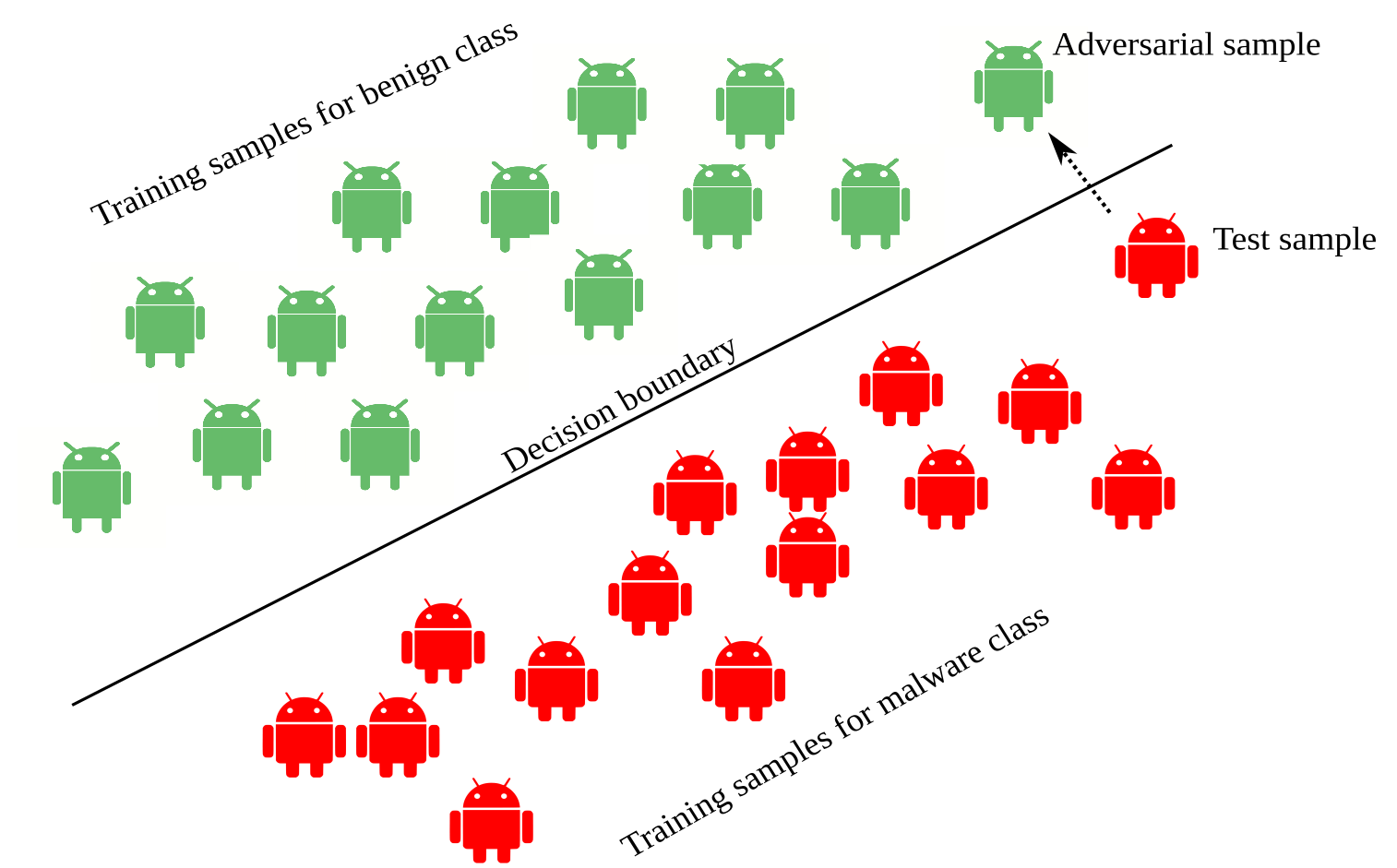
Figure 1: A conceptual representation of evasion attack in a linear malware classifier where a test sample of malicious nature is misclassified as benign after performing a perturbation,

Evolution in designing defenses against adversarial models- Adversarial machine learning has evolved from the initial advances in image-based datasets like MNIST, CIFAR, and ImageNet to malware datasets like binary formatted android package kit (APK) files, application source code, and API calls. However, with the change in dataset format, adversarial machine learning introduces challenges in designing attack and defenses [5, 24, 18, 25, 26]. The major challenges are highlighted below:

1. Feature representation is fixed (pixels) in image classifiers, whereas malware lacks a standard feature representation. Therefore, an adversary has an immense leeway in altering code or modifying files in the application to circumvent detection by the classifier.

2. Features used in malware image classifiers are real, continuous, and differentiable, whereas discrete features represent malware in non-image data.

3. A perturbed image can be visually inspected, but it is challenging to measure if a perturbation has altered the functionality, intrinsic property of non-image data, or has preserved the maliciousness of the application.

4. The adversarial sample of a malware application should also be executable. The perturbation applied to the sample should not break the code structure of the application.

The paper is organized as follows: First, we provide the relevant background on android malware classifier and how to model a threat in Section 2. Our goal is to build a robust defense against adversarial attacks. However, before this, we must learn to capture the patterns behind adversarial examples. It is also essential to understand the reasoning behind the vulnerability of machine learning classifiers. In Section 3, we describe some of the most prevalent hypotheses on adversarial vulnerability. Image data is more popular in the study of adversarial learning, and therefore it also formed the basis of the earliest studies on adversarial learning. In Section 4, we present the foundational works on adversarial attacks and defenses proposed on the image dataset. Next, we detail the methodologies for android malware evasion attacks and defenses in Section 5. We capture the learnings of the surveyed papers and share essential guidelines in Section 6 and potential research direction for building defenses against adversarial attacks in Section 7.

2 Relevant Background

2.1 Android Malware Classifiers

Android malware classifiers are machine learning models trained on features extracted from android apps (see Figure 2). These apps are packaged in APK file format for distribution and installation. The files in an APK package characterize the behavior and operation of an android app (see Table 1). A standard file used by the classification model during feature extraction is the AndroidManifest.xml. This configuration file consists of a list of activities, services, and permissions used to describe the intentions and behaviors of an android application. Similarly, classes.dex file references any classes or methods used within an app.

Table 1: Structure of an Android Package Kit (APK)

File & Directory	Type	Description
META-INF	dir	APK metadata
assets	dir	Application assets
lib	dir	Compiled native libraries
classes.dex	file	App code in the Dex file format
res	dir	Resources not compiled into resources.arsc
resources.arsc	file	Precompiled resources like strings, colors, or styles
AndroidManifest.xml	file	Application metadata — eg. Rights, Libraries, Services

Figure 2: A system diagram of an android malware classifier with evasion attack.

2.2 Feature Extraction

Static, dynamic, or hybrid analyses are common mechanisms for feature extraction. Static analysis does not require running the executable file and instead relies on tools like Androguard, APKTool, Backsmali, or Dex2jar to decompile APK file and extract features like permission (request and use), intent, component (activity, content provider), environment (feature, SDK, library), services, strings, API calls, data flow graphs, and control flow graphs. Vectorized forms of these features, predominantly in string format, can subsequently train an ML classifier, including a neural network model. Features are converted into vectors using one-hot encoding or word vectors using models like Bag-of-Words [27], Word2Vec [28], Glove[29] to transform the text into vectorized representation. Extraction of static features is computationally inexpensive and fast [30], however, falls short when a malware employs encryption or obfuscation technology [31].

In contrast, dynamic analysis involves running the app in a virtual environment or a real machine and monitoring its behavior to extract dynamic features. Some dynamic features represent the intrinsic behavior that is resistant to app obfuscation [2]. For example, system calls, app patterns, privileges, file access details, opening of services, information flows and network traffic. A hybrid method[32] combines features extracted from both static and dynamic analysis to improve the performance of the classifier [33].

In an image-based classifier, static features from AndriodManifest.xml and classes.dex files are converted to RGB or gray-scale images while preserving the local and global features of the APKs [34]. These image features represent binaries of an android app and are used to train a convolutional neural network (CNN) based malware classifier.

Table 2: Notations used in the paper

Notation	Description
$F$	Classifier
$Z$	Set of input object (eg. an image, an application), z$\in$ Z is a sample.
$X$	Set of d-dimensional feature representation of Z, x $\in$ X is a sample
$Y$	Set of label of input dataset, y$\in$ Y is a label of a sample.
$\theta$	Model parameters
$f(x)$	Classifier output decision
$f^{\prime}(x)$	Classifier decision learnt from surrogate dataset
$J(\theta,X,Y)$	Loss function of the classifier
$x*$	Feature of perturbed adversarial sample
$z*$	Perturbed adversarial object
$t$	Target label of an adversary
$\delta_{x}=x*-x$	Perturbation vector
$||.||_{p}$	Lp distance norm (p=0,2,$\infty$ for L0,L2,L$\infty$)
$h,\lambda,k$	Parameters of kernel density estimator
$\nabla_{x}$	Gradient with respect to $x$
$\epsilon$	Constant
$Z(x)$	Logits or unnormalized probabilities before softmax
$(a)^{+}$	max(a,0)
$CLN$	Set of original samples
$ADV$	Set of adversarial samples
$\lambda^{\prime}$	Tradeoff parameter
$m^{\prime}$	Total number of samples in a single mini-batch
$k^{\prime}$	Total number of adversarial examples in each mini-batch
$\mathcal{T}$	Set of available transformations

2.3 Definitions

Here, we define a list of terminology mentioned throughout the paper. Also, see Table 2 for a list of symbols used.

Adversary and Defender: An adversary, also called the attacker, attempts to fool the classifier by producing a misclassification. A defender, on the contrary, develops security defenses against adversarial attacks.

Classifier: A classifier is a machine learning model designed to make a classification decision. Examples of models include support vector machines, feed-forward neural networks, or convolutional neural networks (CNN).

White box and black box attacks: In a white box attack, an adversary has access to the information on architecture, training data, model parameters, hyper-parameters, and the loss function of a target classifier. In a black-box attack, the adversary has no such knowledge about the classifier during an attack.

Perturbation: A perturbation is a carefully crafted noise that can be added to the input dataset to fool the classifier. Manipulation can occur by adding or removing code from the app source code to misclassify the malware as benign. For images, the perturbation vector can modify pixel values. The goal of an adversarial evasion attack is hence to find the minimal perturbation that modifies the classifier decision on an input sample and can be stated formally [8] in Eq. 1:

$$\textnormal{arg~{}min}_{\delta x}||\delta x||~{}\textnormal{s.t.}~{}F(x+\delta x)=t$$ (1)

Here, $||.||$ is the norm to compare the original input and adversarial samples. $\delta x$ is the perturbation added to the sample $x$ to create an adversarial sample $x*=x+\delta x$, leading to misclassification as $t$. Heuristics, brute force, or optimization algorithms can be used to obtain such minimal perturbations. Fig 3 shows how a test sample is perturbed in feature space using three different attack type for producing misclassification.

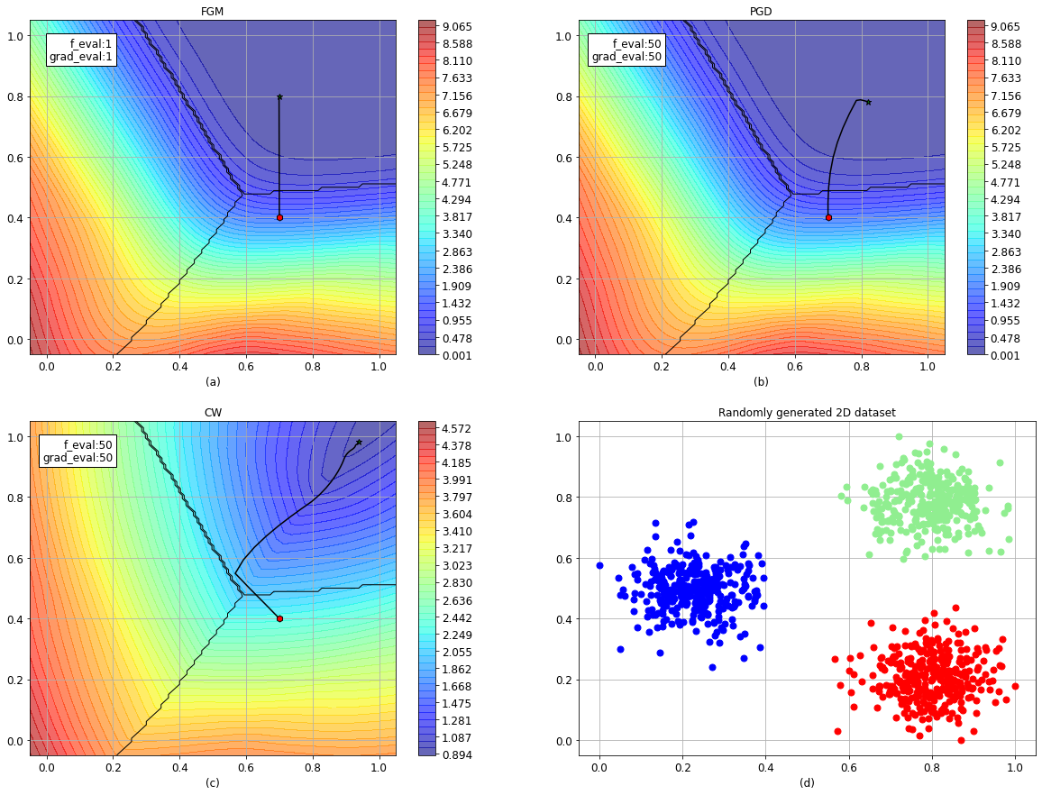
Figure 3: Representation of evasion attack in a multi-class classifier using SecML [35] and Cleverhans [36] framework. The toy 2D dataset consists of 3 clusters of points generated randomly using a normal distribution. We train a 2-layer neural network for making multi-class classification, and obtain an accuracy of $99\%$ on the test set. We then perform FGM, PGD and CW attacks on the classifier for generating adversarial samples. Figures (a), (b) and (c) show how an initial sample (represented by a red hexagon) belonging to one class is perturbed in its feature space to its adversarial sample (green star) for misclassification using the attack. f_eval and grad_eval represent the number of evaluations of the function and its gradient for performing the attack. See Section 4 for details on the FGM, PGD and CW attacks.

2.4 Threat Model

The adversarial goal is to perform evasion attacks that compromise the integrity of a classifier by making targeted (misclassifying a particular set of input) or indiscriminate (misclassifying any sample) attacks [16, 13]. An adversary’s knowledge about the target classifier can be partial or complete on the training data, feature set, learning algorithm, parameters, and hyper-parameters. An adversary’s capabilities defines how they can exploit the classifier at train or test time [16] or the challenges they can overcome during sample perturbation [18]. This survey focuses on both white-box and black box attack at test time.

2.5 Example on android evasion attack

Here, we describe a simple experiment on the evasion attack of an android malware classifier to demonstrate the severity of an adversarial attack on the accuracy of a classifier. For building the android malware classifier, we use the Drebin dataset [1], which consists of $12000$ benign and $550$ malicious samples. We split the dataset into a train-test set and trained a linear support vector machine (LSVM). We obtain a classification accuracy of $95.04\%$ with an $89.09\%$ F1 score on the test set.

We produce adversarial samples against the SVM classifier using a gradient-based attack [5]. Drebin represents the android apps as one-hot encoded vectors of various permissions in AndroidManifest.xml. Thus, at each iteration of the attack, we modify one feature of the android app from $0$ to $1$. It means that we add new features to an android app for its modification. Perturbation $\epsilon$ limits the number of features permitted for modification during an attack. To evaluate the robustness of the classifier against the evasion attack, we plot a security evaluation curve [See figure 4] using SecML [35]. The curve plots the classification accuracy against the increasing perturbation $\epsilon$ value. Figure 4 shows how changing a mere $12$ number of features reduces the classification accuracy of the classifier by half. This simple example model demonstrates that an evasion attack on malware classifiers is a significant security threat.

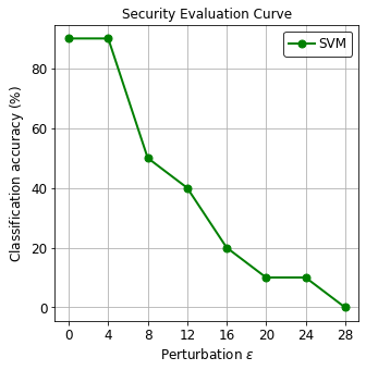
Figure 4: A security evaluation curve showing the reduction in classification accuracy of an android malware classifier as the perturbation $\epsilon$ (number of feature modification) is increased.

3 Finding patterns in classifiers vulnerability to adversarial attack

Adversarial attacks exploit aberrations in the learned parameters of the classifier. Earlier, the hypothesis was that the presence of ‘blindspots’ in neural networks caused adversarial vulnerability of classifiers [4]. Szedy et al. argued that the adversarial examples represented the low probability pockets in the network manifold created due to insufficient training examples. If an adversarial sample existing in that manifold is supplied during test time, the model will fail to classify it. Such lower-probability pockets were the result of high non-linearity in deep neural networks.

Contrary to the non-linearity hypothesis of [4], Goodfellow et al. [6] have argued that the resemblance of neural networks to linear classifiers in high dimensional space is the reason behind a classifier’s inability to determine adversarial samples accurately. Linear classifiers cannot resist adversarial perturbation. If a linear model $y=\theta^{T}x$ receives a modified input $x^{\prime}$ such that $x^{\prime}=x+\delta$, the new activation $w^{T}x^{\prime}$ in the classifier is expressed as:

$$\theta^{T}x^{\prime}=\theta^{T}(x+\delta)=\theta^{T}x+\theta^{T}\delta$$ (2)

Equation 2 shows that adding an adversarial perturbation of $\delta$ increases the activation of the model by $\theta^{T}\delta$. If the input is high-dimensional, a slight input perturbation can create a large perturbation in output.

However, Tanay et al.[37] argued that this linear view of neural network poses several limitations primarily because the behavior of a neural network and a linear classifier is different. They verified that activation function in the neural network units does not grow linearly, as explained in [6] by finding adversarial examples that resist adversarial perturbation in a linear classifier. Instead, they propose that adversarial examples exist when the class boundary lies close to data. Because of this, modification of points from the data manifold towards the boundary will cause the data to mis-classify. Overfitting could be the rationale behind this behavior, and they argued that proper regularization could address this phenomenon.

The previously mentioned hypothesis treats the adversarial behavior of the neural network as a separate goal independent from the network’s goal of accuracy. They argued that adversarial behavior of a classifier can be tackled with regularization or input (or, output) pre-processing (or, post-processing) [4, 6, 37]. However, recent work by Ilyas et al. [38] claimed that adversarial vulnerability is the result of the model sensitivity towards features generalization. They argued that classifiers train to maximize accuracy regardless of the features they use. Because of this, the model tends to rely on ‘non-robust’ features for making decisions allowing possibilities of adversarial perturbations. This hypothesis also explains the presence of adversarial transferability.

Though the verdict is yet not unanimous in explaining the cause behind adversarial vulnerability, this new hypothesis on adversarial vulnerability being the intrinsic property of data and result of our goal for generalization has paved the way for new research in building defenses [39, 40].

4 Evasion attacks and defenses: Patterns in images

4.1 Evasion attacks

The earliest experiments demonstrated adversarial attacks on linear classifiers. They successfully fooled spam-email classifiers by obfuscating common spam words or by adding non-spam words to the content of spam emails [41]. It was inferred that only linear classifiers are vulnerable to adversarial attacks and non-linear classifiers are robust against evasion attacks [42]. Biggio et al.[5] countered this assumption by evading non-linear support vector machines (SVMs) and neural networks.

4.1.1 White-Box Attack

Gradient attack: In [5], Biggio et al. present a gradient descent-based method for finding adversarial samples of both MNIST digits and PDF malware. They perform an evasion attack on SVM classifiers by computing the gradient of the classifier’s discriminant function on the input sample such that it reverses the decision of the classifier. They add a density estimator to penalize the optimization function.

$$x^{*}=\textnormal{argmin}_{x}\Big{(}f^{\prime}(x)-\frac{\lambda}{n}\sum(k(x-x_{i})/h)\Big{)}$$ (3)

subject to $d(x,x*)\leq d_{max}$ which is the upper limit on changes permitted on a feature. This approach was successful in evading both linear and non-linear classifiers, unlike previous works on evasion attacks that were limited to linear and convex classifiers[42].

L-BFGS Attack: In 2014, Szedel et al.[4] show the vulnerability of neural network classifiers against modified images. They observe that even though neural networks generalized well to the test dataset, they were not entirely robust against adversarial inputs. As a result, they formulate the evasion attack as an optimization algorithm and propose a solution using a box-constrained limited memory-Broyden–Fletcher–Goldfarb–Shanno algorithm (L-BFGS).

$$\textnormal{min}_{\delta}\Big{(}c||\delta||_{2}+\textnormal{loss}_{f}(x+\delta,t)\Big{)}$$ (4)

subject to $x+\delta\in[0,1]^{n}$. The goal of the optimization in Equation 4 is twofold. The first is to perform a linear search to find the constant $c$ that locates a minimally perturbed sample. The second is that the modified image $x+\delta$ must still normalize between $0$ and $1$. This method can be computationally slow and not scale to large datasets. Additionally, this paper presents two compelling properties of adversarial examples. First, the adversarial examples generated from a classifier could evade another classifier trained with the same training dataset but different parameters. Second, they could also fool models trained on a different disjoint training set. These two properties of adversarial samples came to be known as “cross-model generalization” and “cross-training set generalization.”

FGSM attack: In [6], Goodfellow et al. propose a gradient-based approach to generate adversarial examples against neural nets similar to [5]. However, unlike [4] that optimizes the perturbation for $L2$ distance and solves an optimization problem, this method is optimized for the $L\infty$ metric and assumes a linear approximation of the model loss function. The optimal max-norm perturbation uses the following expression:

$$\delta=\epsilon*\textnormal{sign}(\nabla_{x}J(\theta,X,Y))$$ (5)

Equation 5, also called the fast-gradient sign method (FGSM) for an un-targeted attack, finds the perturbation by increasing the local linear approximation of the loss function. FGSM is ‘fast’ because the loss gradient computes once and modifies the input perturbation of single-step size $\delta$. In a targeted attack, the target label $T$ in the loss function can obtain an adversarial sample by using:

$$x*=x-\epsilon~{}\textnormal{sign}(\nabla_{x}J(\theta,X,T))$$ (6)

Iterative FGSM attack: While FGSM can be fast in producing adversarial samples, it is not optimal. FGSM has limitations since it does not produce minimally perturbed adversarial samples. Kurakin et al. [7] propose an iterative method to produce an optimal perturbation using the fast gradient sign method. They compute the sign of the gradient of the loss function with respect to the input, multiply it by the step $\alpha$, and clip the output to $\epsilon$ so that the transformed input is on the $\epsilon$ neighborhood. They repeat this process with multiple smaller steps of $\alpha$. The number of iterations are heuristically selected to be between $\textnormal{min}(\epsilon+4,1.25~{}\epsilon)$. This attack is also called Projected Gradient Descent (PGD) attack. Mathematically, Equation 7 represents the iterative gradient sign method.

$$x*=x_{n-1}-\textnormal{clip}_{\epsilon}(\alpha~{}\textnormal{sign}(\nabla xJ(\theta,x_{n-1},y))$$ (7)

RAND FGSM attack: Tramer et al. [12] propose a randomized fast gradient sign method (RAND+FGSM) by introducing a gaussian perturbation to the input before applying the single-step FGSM attack. This method produces a more powerful perturbation for fast gradient attacks.

$$x*=x^{\prime}+(\epsilon-\alpha).sign(\nabla_{x^{\prime}}J(x^{\prime},y))$$ (8)

where, $x^{\prime}=x+\alpha.sign(N(0^{d},I^{d}))$ and $\alpha<\epsilon$.

JSMA attack: In [8], Papernot et al. generate a novel adversarial attack using $L0$ distance metric to minimize perturbation of the input. They utilize salient maps to select a subset of input features to be modified to produce misclassification. They propose a method based on forward derivative, represented by Jacobian matrix of the deep neural network, $J_{F}(x)=\frac{\partial F(X)}{\partial X}$. For all pairs of features $(p,q)$ in the input dataset, the following values are omputed to obtain saliency,

$$\alpha=\frac{\partial F_{t}(X)}{\partial X_{p}}+\frac{\partial F_{t}(X)}{\partial X_{q}}$$ (9)

$$\beta=\sum_{j\neq t}(\frac{\partial F_{j}(X)}{\partial X_{p}}+\frac{\partial F_{j}(X)}{\partial X_{q}})$$ (10)

given, $\alpha>0$ and $\beta<0$, features $p$ and $q$ are modified iteratively until a misclassification is obtained or a maximum iterations is reached. This method is known as Jacobian-based Saliency Map Attack (JSMA).

C&W attack: In [11], Carlini et al. devise one of the strongest attacks, using $L0$, $L2$ and $L{\infty}$ distance metrics. This attack, known as the C&W attack, demonstrates the vulnerability of one of the most widely accepted defense strategies against adversarial attack at that time– defensive distillation [43]. The C&W attack is similar to [4]; however, the difference lies in the use of the objective function. While L-BFGS used cross-entropy loss, the C&W attack uses margin loss, which is more efficient than cross-entropy loss. Here, we formally define this adversarial attack:

$$\textnormal{minimize}~{}||\delta||_{p}+\lambda^{\prime}.f(x+\delta)$$ (11)

such that $x+\delta\in[0,1]^{n}$. Here, $c$ is the minimum value that can achieve two goals– minimize $\delta$ or $f(x+\delta)$, i.e., successfully produce a target label and obtain minimal perturbation while making an attack. The value of $c$ is selected to achieve both goals. This optimization is reformulated with seven different objective functions such that $C(x+\delta)=t$ iff $f(x+\delta)\leq 0$. After empirical evaluation on several functions, the following function is proposed:

$$f(x*)=[\textnormal{max}_{i\neq t}Z(x*)_{i}-Z(x*)_{t},-k]^{+}$$ (12)

Here, $k$ encourages the optimizer to find an adversarial example with high confidence. The constraint for $x+\delta$ to be in the interval of $[0,1]$ requires box constraint optimization solution. Hence, a ‘change of variable’ method removes the box constraint and solves the optimization using a modern optimizer like Adam. A variable $w$ replaces $\delta$ such that the L2-norm attack is expressed as:

$$\textnormal{minimize}~{}||\frac{1}{2}(\textnormal{tanh}(w)+1)-x||_{2}^{2}~{}+c.f(\frac{1}{2}(\textnormal{tanh}(w)+1)$$ (13)

Since L0 attacks are non-differentiable forms of attack, they use an iterative method like JSMA [8] but with one prime difference. JSMA method obtains the features required to be modified using saliency maps and iterates this process till the misclassification occurs. In this approach, Carlini et al. take the complete set of pixels and identify the features that do not have much effect on the classifier decision. By process of elimination, they obtain the set of features that when modified creates adversarial sample.

For $L\infty$ attacks, they iteratively solved

$$\textnormal{minimize}~{}\sum_{i}[(\delta_{i}-\tau)^{+}]+c.f(x+\delta)$$ (14)

where, $\tau$=1 in first iteration. If $\delta_{i}<\tau$, $\tau$ is reduced by a factor of 0.9.

DeepFool attack: DeepFool is an iterative L2-attack designed to produce minimally perturbed samples proposed by Moosavi et al. [9]. For a linear binary classifier, the minimal perturbation required to produce an adversarial example of a sample $x$ is obtained by finding the projection of the sample on the classifier’s decision boundary, a hyperplane $F:\theta^{T}x+b=0$. This projection is given by $-\frac{f(x0)}{||\theta||_{2}^{2}}\theta$. For a general curved decision surface, a linear approximation is obtained using a small linear step of $\nabla f(x)$ at each iteration $x_{i}$.

Using the closed form solution of perturbation $\delta$ for linear case, the perturbation $\delta$ for general case is expressed as:

$$\delta_{i}=-\frac{f(x_{i})}{||\nabla f(x_{i})||_{2}^{2}}\nabla f(x_{i})$$ (15)

The modified sample $(x*)$ is obtained by adding $\delta$ from equation 15 to $x_{i}$. If the classifier wrongly predicts the perturbed sample, the adversarial sample is obtained. Otherwise, the procedure is repeated. For multi-class classifiers, similar projection holds with addition of multiple decision boundaries. If the decision boundaries are curved, linear approximations should be made.

Table 3: Summary of attack and defense papers (image) in the survey

	Attack		Defense							Dataset
Paper	Blackbox	Whitebox	Optimization	Adv. Training	Non-linearity	Ensemble	Weight regularization	Adversarial detection	Generative Modeling	MNIST [44]	CIFAR [45]	ImageNet [46]	GTSRD [47]	Others
Gradient descent evasion attack [5]
L-BFGS [4]
FGSM [6]
PGD [7]
RAND+ FGSM [12]
JSMA [8]
C&W [11]
DeepFool [9]
Practical Black-box [10]
ZOO [15]
Generative Black Box [48]
Deep Contractive Network [49]
Learning with adversary [50]
Defensive and Extended Distillation [43, 51]
Feature squeezing [52]
Detection Network [53]
MagNet [54]
Statistical Detection Network [55]
Blocking transferability [56]
Gradient regularization [57]
Defense GAN [58]
Adversarial training for free [59]

4.1.2 Black-Box Attack

While an adversary exploits all the information of a classifier in white box attacks, practically such amount of information is not available. In real scenarios, the attacker can have some information regarding classifier or training data but not all. They mostly have to attack a model without prior knowledge on its loss function, parameters or training data. They can however access to the model output given some test input.

Practical black-box attack: In [10], Papernot et al. demonstrate the first black-box attack that fooled a remotely hosted deep neural network (Oracle). The proposed method consists of substitute model training and adversarial sample crafting.

1. Substitute model training: The adversary learns a substitute model that mimics the decision behavior of the oracle (target classifier) by using synthetic dataset labeled by the oracle.

2. Adversarial sample crafting: Once the substitute model is developed, adversarial transferability enables the attack on oracle using adversarial samples from the substitute model.

The first step in substitute model training is to select an architecture for the model. An adversary can make an educated assumption by observing the behavior of the target model (oracle), its input data and output labels. The second step is to develop synthetic datasets. An adversary can hypothetically query Oracle with infinite number of inputs and approximate the substitute model by training the input-label set, ensuring that the substitute model mimics the behavior of Oracle. However, there might not be enough training samples with the adversary, which a Jacobian-based data augmentation method can address. It generates datasets based on the gradient of the label assigned by a model for the input sample. The gradient identifies how the Oracle output varies around some initial point and moves towards that direction to generate inputs that can capture the behavior of the Oracle. Let, $S_{p}$ represent the initial dataset; then the Jacobian dataset augmentation augments the dataset into $S_{p+1}$.

$$S_{p+1}=\{x+\eta.\textnormal{sign}(J_{F}[O(x)]):x\in S_{p}\}US_{p}$$ (16)

where $\eta$ is a parameter of the augmentation that defines the step size to move in the direction identified by the Jacobian matrix. By repeating these three steps: querying Oracle for a label, training the substitute model, and generating a synthetic dataset, an adversary can create a substitute model that can mimic the Oracle decision behavior. Adversarial samples are generated using any white-box attack upon obtaining the substitute model. Such samples can also evade the classifier of the Oracle following the transferability property of adversarial attacks.

ZOO attack: In [15], Chen et al. propose the zeroth-order optimization attack (ZOO) for both text and image dataset. This attack does not use a substitute model for generating adversarial samples. Instead, it approximates the gradient of the target model by using the information of input and confidence scores provided by the output. Similar to [11], they state the following objective function as the optimization goal.

$$\textnormal{minimize}~{}||x-x_{0}||_{2}^{2}+c.f(x,t)$$ (17)

subject to $x\in[0,1]^{n}$. The expression for $f(x,t)$ of Equation 12 is modified to suit a black box attack by including the output of the classifier ($F(x)$) in place of logits $Z(x)$:

$$f(x,t)=\textnormal{max}[\textnormal{max}_{i\neq t}log(F(x)_{i})-log(F(x)_{t}),-k]$$ (18)

ZOO are derivative-free methods and use the value of objective function at two close points $f(x+h)$ and $f(x-h)$ to estimate gradients.

Generative attack: In [48], Zhao et al. use generative adversarial network (GAN)[60] for producing adversarial samples. The generator is trained to learn a data generating distribution mimicking input $x$ from random vectors $z\in R^{d}$. Using an inverter network ($I$), the input sample is mapped to the generator labeled with incorrect output. Mathematically, the adversarial sample is given by:

$$x*=G_{\theta}(z*)~{}\textnormal{where}~{}z*=\textnormal{argmin}_{z^{\prime}}||z^{\prime}-I_{\gamma}(x)||$$ (19)

such that $f(G_{\theta}(z^{\prime}))\neq f(x)$. This approach utilizes input instances for creating adversarial samples and does not depend on an attack algorithm.

4.2 Adversarial defenses

Defending against an adversarial attack either involves detecting an adversarial sample and rejecting it called adversarial detection or building a robust classifier that is, by design, resilient against evasion attacks. Several attack algorithms have shown that no defense methods are robust enough to handle all kinds of attacks [11]. An adversary can always exploit the limitations of defenses by carefully crafting new attacks. Here, we explain some widespread defense methodologies proposed in the literature.

Non-linear element for defense: In[6], Goodfellow et al. argue that the linearity introduced in non-linear networks by elements like ReLU is the reason behind adversarial vulnerability. Therefore, they propose to use radial basis functions (RBF) instead of ReLU. Though the modified network is successful in resisting adversarial attacks, they are resistant only to weaker forms of attacks [11].

Buckman et al. [61] derive an encoding method inspired from the work of PixelRNN [62] and apply a non-linear and non-differentiable activation to the input. They propose an encoding method called Thermometer Encoding to discretize the image into one-hot vectors. Such pre-processed input train a classifier with an assumption that non-linear representation will break the linear behavior of the model. This defense method is also resistant to weak attacks only.

Adversarial training: Adversarial training [6] is a popular defense method using a mixture of normal and adversarial examples for training. The additional set of adversarial examples provides information regarding adversarial ‘outliers’ to improve model performance against adversarial attacks. Equation 20 shows the objective function for adversarial training where $J^{\prime}$ is the modified loss function.

$$J^{\prime}=\lambda^{\prime}J(\theta,x,y)+(1-\lambda^{\prime})J(\theta,x+\epsilon~{}\textnormal{sign}(\nabla_{x}~{}J(\theta,x,y))$$ (20)

Limitation of adversarial training: Adversarial training can overfit to perturbation samples used for training [63] and is, therefore, unsuitable for scalability [7]. An ensemble adversarial training method can address this limitation [12] where the training set is augmented with different perturbation obtained from attacks on several pre-trained models to avoid the degeneration of minimum of an adversarial training with single perturbation. Kurakin et al. address the second limitation in [7] by proposing an improved version of adversarial learning suitable for large-scale datasets like ImageNet. The input datasets are grouped into batches of original and adversarial samples before training. The objective function is additionally modified to address the relative contribution of adversarial examples in each batch.

$$L=\frac{1}{(m^{\prime}-k^{\prime})+\lambda^{\prime}k^{\prime}}(\sum_{i\in CLN}L(x_{i}|y_{i})+\lambda^{\prime}\sum_{i\in ADV}L(x^{adv}_{i}|y_{i}))$$ (21)

Even with limitations, adversarial training still performs reasonably better than most defense methods and withstand strong attacks [59, 64, 65].

Gradient Optimization: Gu et al. [49] conclude that the problem of adversarial attack can be solved only by finding a new training process and optimization algorithm. They propose a deep contractive network, which is a generalization of a contractive autoencoder, to make adversarial perturbation difficult for an adversary[66]. A contractive autoencoder has the same architecture as a standard auto-encoder; however, it also introduces a penalty for minimizing the Jacobian of the lower-dimensional representation of the input.

$$J_{DCN}(\theta)=\sum_{i=1}^{m}(L(t(i),y(i))+\sum_{j=1}^{H+1}\lambda_{j}^{\prime}||\frac{dh_{j}^{(i)}}{dh_{j-1}^{(i)}}||_{2})$$ (22)

where, $H+1$ indicates the number of layers in the network where $h_{H+1}=y$.

Instead of retraining a model with adversarial samples with adversarial training, Huang et al. [50] formulate a single min-max problem for building a robust model. The goal of the optimization is to maximize misclassification and produce perturbed samples while minimizing the overall misclassification.

$$\textnormal{min}_{f}\sum_{i}\textnormal{max}_{||\delta_{i}\leq c||}L(f(x_{i}+\delta_{i}),y_{i})$$ (23)

where, the parameter $c$ controls the perturbation magnitude. This objective function trains the network for the worst examples.

Ross et al. [57] formulate that networks equipped with input gradient regularization are more robust to adversarial attacks than unregularized networks. Drucker and Le Cun proposed input gradient regularization as double backpropagation [67]. Double backpropagation aims to improve neural network training by minimizing the rate of change of output with respect to the input. Using this definition, they propose the following objective function:

$$\theta*=\textnormal{argmin}_{\theta}J(y,y^{\prime})+\lambda^{\prime}||\nabla_{x}J(y,y^{\prime})||_{2}^{2}$$ (24)

This regularization ensures that the output prediction does not change drastically on a slight input modification.

Weight regularization: Hinton et al. [68] propose distillation for deep learning to utilize the knowledge acquired by a large and complex neural model and transfer it to a smaller model. Papernot et al. [43] apply the intuition of distillation for improving the resilience of the deep neural networks against adversarial samples. Instead of transferring knowledge to a smaller model, the knowledge obtained from a deep neural network (output probability vectors) enhances its robustness. In distillation, soft labels train a classifier instead of high confidence, hard labels. It reduces the sensitivity of the model with respect to variations in input (Jacobian) which are exploited for generating adversarial samples in [4, 6, 8] . A neural network model is trained with a softmax output layer at temperature $T$. The training set consists of samples $(X,Y)$ where $Y$ are hard labels $(0~{}or~{}1)$. The output of this model obtains the probability vectors given by equation for a smooth version of the softmax in Equation 25:

$$F(X)=[\frac{\textnormal{exp}(z_{i}(X)/T)}{\sum_{l=0}^{N-1}\textnormal{exp}(z_{l}(X)/T)}]_{i\in 0...N-1}$$ (25)

A distilled model is trained with same architecture, alibi new training samples $(X,F(X))$ and the softmax temperature, $T$. For test time $T=1$ is used, similar to the original distillation paper [68].

Defensive distillation [43] is successful against FGSM [6] and JSMA [8] attacks but failed against new attacks proposed by Carlini et al. [11]. Papernot et al. [51] propose a variant of defensive distillation to address the limitations by training the distilled model with additional information of uncertainty from the first model. Their approach was motivated by two lines of defense previously proposed in the literature:

1. Training a classifier to model the adversarial inputs by introducing an outlier class [55, 56]

2. Quantifying uncertainty of the model decision using stochastic inference [69]

While prior defenses involved modification of neural network, Xu et al. [52] propose a detection method by making no changes to an existing model and only modifying the input. They reduce the input dimension, offering fewer degrees of freedom to the adversary. They apply two feature squeezing methods to test images: reduction of color depth and spatial smoothing of images. Both of these methods reduce the pixel (dimension) of an image. An image is passed through a classifier during testing to generate an output probability vector. The same test image is passed through feature squeezing networks and then to the same classifier, producing a probability vector. Comparing these two prediction vectors with a $L1$ norm shows how different the predictions are. An adversarial test sample produces a significant difference in prediction compared to the unmodified test sample, thus providing the detection result.

Adversarial detection: Metzen et al. [53] also propose a detection network for identifying adversarial samples by augmenting the primary classifier with smaller adversarial detector networks. The task of this sub-network is to detect adversarial examples from the regular samples for a specific adversary. First, they train a classifier on unperturbed samples and then generate the perturbed samples for a specific adversarial attack. They augment the training dataset with the corresponding adversarial dataset and train the detector network for classifying the adversarial samples freezing the primary classifier. The detector network can be attached at various classifier layers decided on experimental evaluations.

In [55], Grosse et al. utilize the statistical properties of adversarial examples for detection. They hypothesize that adversarial examples exist because of the difference between the actual data distribution and the empirical data distribution obtained from the train set. While adversarial sample could be consistent with the real data distribution, it does not follow the training distribution because of a limited number of samples at hand. Using statistical tests, the difference between such two samples can determine whether they are sampled from the same distribution. Grosse et al. measure the statistical distance between the training and manipulated data and observe a significant distance between the samples as the attack parameters increase. With statistical testing, we can estimate whether any overall adversarial examples are present in the dataset. However, we cannot predict whether a single specific input is adversarial or not. Hence, they modify their learning model to incorporate an additional outlier class for adversarial examples and train the model to classify them. They train the initial model on clean training examples, generate adversarial samples, and then train a new model by augmenting the original training samples with the adversarial samples labeled as outlier class. The goal of the ML classifier is not just to identify the true class of the input but also to classify if it is an adversarial sample.

Another defense approach called MagNet is proposed by Meng et al. [54] that neither modifies the classifier nor creates adversarial samples. Instead, it uses detector and reformer networks. The task of a detector network is to discard such samples located far away from the data manifold learned by the classifier using training samples. If the adversarial sample is close to the boundary, then the reformer network transforms the adversarial sample to an original sample. They use auto-encoder to achieve this. MagNet was able to recover classification accuracy with all attacks except C&W attack. To address the limitation with C&W attack, they propose a defense via diversity method. In this approach, they train several auto-encoders and randomly pick one at a run time for making the prediction.

Because of the transferability property of adversarial attacks, even a black box system can be easily fooled by generating attacks on substitute models. Hosseini et al. [56] propose a method to block this transferability behavior of adversarial attack. They devise a training method that identifies adversarial samples as the perturbation increases. Firstly, they train a classifier to produce adversarial samples. Once the adversarial samples are obtained, the output label of the images is augmented to include a NULL label. The original and adversarial images are labeled with this additional parameter. The value of this NULL label depends on the perturbation applied to create the sample, computed as $p_{NULL}=f\frac{||\delta X||}{|X|}$. Depending on the value of NULL label, other prediction values are modified following the heuristic: the ground truth is modified from $q$ to $q(1-p_{NULL})$ and other labels to $\frac{(1-q)(1-p_{NULL})}{K-1}$ where $K$ are the number of output classes. Finally, the model is trained with both the unmodified and perturbed samples to maximize test accuracy and detection of adversarial samples.

$$\theta^{*}=\textnormal{argmin}_{\theta}\lambda^{\prime}L(X,Z;\theta)+(1-\lambda^{\prime})L(X+\delta X,Z_{A};\theta)$$ (26)

where, $Z_{A}$ is the output probability vector labeled with NULL.

Generative model for defense: Samangouei et al. [58] use the generative property of GAN [60] in building a defense against adversarial attacks. Generator, a multilayer perceptron, mimics the distribution of unperturbed training samples in GAN. This method minimizes the reconstruction error between the generator and the test image. This projection of the test image is fed to the classifier for prediction instead of the given test sample. The intuition behind this is that an unperturbed sample will be closer to the distribution learned by generator $(G)$, and an adversarial sample will be far away from the range of $G$.

$$z^{*}=\textnormal{min}_{z}||G(z)-x||_{2}^{2}$$ (27)

GAN-Defense can be used with any classifier as it does not modify the structure of the model. More importantly, it does not rely on any attack to improve its robustness; hence it is suitable for all kinds of attacks.

5 Evasion attack and defenses: Patterns in android malware classifiers

Evasion attack in malware introduces additional constraints (see Section 1), which challenges the modification of real objects vis-a-vis the attack-optimized feature vector. This modification is a straightforward pixel transformation in image dataset. However, a feature space attack must ensure that the inverse feature mapping exists for malware. Let us consider $Z$ to be problem space object (eg. android APK file), $z\in Z$ be any object with a label $y\in Y$, $\phi:Z\rightarrow X\subseteq R^{n}$ be the feature mapping function that transforms the problem space object $z\in Z$ to an n-dimensional feature vector $x\in X$ , such that $\phi(z)=x$. Consider $x$ represents one-hot encoded binary vectors. Feature-space attack modifies the feature $x\in X$ with assigned label $y\in Y$ to $x*$ with a perturbation to classify it as $t\in Y,t\neq y$. The challenge with malware evasion attacks is to find the corresponding adversarial object by applying some transformation to $z$ so that $\phi(z*)=x*$ where $x*$ is the adversarial feature vector. Thus, the transformed feature vector $x*$ must correspond to an executable adversarial real space application $z*$. For example, FGSM for malware proposed by [70] not just adds the perturbation to the input but constrains the output to a projection that outputs only a possible set of values. If the features are binary encoded one-hot vectors, the features can only have $1$ or $0$ regardless of the perturbation.

Table 4: Summary of attack and defense research on android malware classifiers

	Attack					Defense						Dataset
Paper	Feature selection	Feature space	Heuristic search	Ensemble	Generative	Adv. Training	Feature Selection	Input processing	Ensemble	Weight regularization	Monotonicity	Drebin [1]	MaMaDroid [71]	Comodo	Androzoo [72]	Contagio	Others
Gradient descent evasion attack [5]
One-and-half classifier [73]
Sec-SVM [74]
Bit Coordinate Ascent (BCA): [13]
Malware Recomposition Variance [14]
MalGAN [75]
SecureDroid [76]
Monotonic Classification [77]
Problem space attack [18]
Android HIV [17]
Hashed Network[78]
DroidEye[79]
Ensemble Classifier [80]
Projected attack [70]
Ensemble defense [81]
Random nullification [82]
Ensemble classifier mutual agreement [83]

5.1 Evasion attacks

Attack using features selection: Grosse et al. use a feature selection method in [13] for producing adversarial samples of android malware targeting a feed-forward neural network classifier. Consider a $M$ dimensional android application represented by a binary vector $x\in\{0,1\}^{M}$. To address the constraints for perturbation in malware, they propose to only add features in AndroidManifest.xml file and restrict the number of features added. They use the forward derivative-based method proposed by [8] for crafting adversarial samples. First, they compute the gradient of the classifier $F$ with respect to input $X$, also called forward derivative and then select a perturbation $\delta$ that maximize the gradient with respect to $X$ i.e. pick the feature $i$ such that $i=argmax_{j\in[1,m],X_{j}=0}F_{0}(X_{j})$. Ideally, the perturbation has to be small so that the modified sample behaves like the original sample. It is easier to inspect this constraint in an image. However, malware samples are represented by discrete and binary features; either a feature is present or absent. Hence, to apply this constraint, based on the forward derivative information, they change one feature of $X$ from $0$ to $1$ and iterate the process until there are a maximum number of changes to the features or the classifier produces a misclassification. This attack is also called the bit coordinate ascent (BCA) attack.

Most evasion attacks for android apps focus on feature modification of AndroidManifest.xml only. Chen et al. [17] propose an automated tool called android HIV for adding perturbations to both AndroidManifest.xml and classes.dex files. To attack the MaMaDroid classifier [71], they extract features from the classes.dex file as Control Flow Graph (CFG). CFG is represented by the sequence of API calls and captures the sequential behavior of an application. For simplifying the representation of API calls, it is abstracted to either family or package level. These features are represented as transition probabilities between different API calls and used in building a Markov chain. To generate an attack on MaMaDroid, they insert API calls in the original smali code to modify this Markov chain. They modify the C&W attack [11] and JSMA attack [8] as follows:

1. C&W attack: C&W attack is given by Equation 28.

   $$\textnormal{minimize}~{}||\delta||_{2}^{2}+c.f(X+\delta)$$ (28)

   where $f(X)=\textnormal{max}[\textnormal{max}_{i\neq t}Z(X)_{t}-Z(X)_{i},-k]$. Specific constraints are added to the C&W attack suitable for modifying the features of MaMaDroid. The first constraint $X+\delta\in[0,1]^{n}$ is the limitation on the value of the feature which should be between $0$ and $1$. The second constraint: $||X_{g}+\delta_{g}||_{1}=1$, $g\in 1...k$, is the limitation on the norm of the features in each family or package of the API call. It also should be equal to $1$. Since the optimization is performed to add a number of API calls, the optimization variable is changed from $\delta$ to $w$ where $w$ is defined by:

   $$\delta_{i}^{g}=\frac{a_{i}^{g}+w_{i}^{g}}{a^{g}+w^{g}}-\frac{a_{i}^{g}}{a^{g}}$$ (29)

   where $w^{g}=\sum_{i}w_{i}^{g}$ and $a_{i}^{g}$ represents the total API calls made by i-th feature in the g-th group. They resort to only addition of API calls.

2. JSMA: Chen et al. modify the JSMA attack to obtain the Jacobian between API call numbers ($A$) and the model output as expressed in Equation 30.

   $$J_{F}(A)=[\frac{\partial F(x)}{\partial X}\frac{\partial X}{\partial A}]=[\frac{\partial F_{J}(X)}{\partial x_{i}}\frac{\partial x_{i}}{\partial a_{i}}]$$ (30)

   After the Jacobian is computed, they form a saliency map of features and iteratively modify the features that have largest saliency value till the misclassification is obtained similar to implementation of [8].

They use the JSMA attack similar to MaMaDroid for attacking the Drebin classifier. Since Drebin directly uses features of the decompiled APK files and does not examine their execution, they add non-executable code samples for creating adversarial samples.

Attack using heuristic search: Yang et al. [14] propose Malware Recomposition Variation (MRV) that systematically performs the semantic analysis of an android malware to compute suitable mutation strategies for the application. Using such strategies, a program transplantation method [84] adds byte-codes to existing malware to create a new variant that successfully preserves the maliciousness of the original malware. Since they perform a semantic analysis of the malware to identify feature patterns before feature mutations, the adversarial sample is less likely to crash or break and preserve the maliciousness. They propose feature evolution and feature confusion attacks for mutating the malware:

1. Evolution attack: The goal of this attack is to mimic the evolution of malware to evade classification. A phylogenetic evolutionary tree analysis [85] is performed on the malware family to understand their evolution of feature representations. Depending on feasibility (modified features) and statistical frequency (number of mutations of a feature) set, they rank different features suitable for mutation. They select the top 10 features for mutation for generating an adversarial sample.

2. Confusion attack: This attack uses mutation of features used by both the malware and benign samples. They first extract essential features of both malware and benign applications using PScout [86] and then create a set of resource features shared by both kinds of apps into a confusion vector set. Features are picked from this confusion set for perturbation.

Yang et al. use transplantation framework [84] to add the feature to the malware app. An organ transplantation framework first identifies a code section to extract and insert into a point of insertion in the app. After insertion, the environment issues of the host are addressed by modifying the code. They present additional strategies for inter-method, inter-component, and inter-app transplantation.

Pierazzi et al. [18] investigate the problem-space attacks and propose a set of formalization by defining constraints on the adversarial examples. They use this formalization to create adversarial malware in android on a large scale. They define the following constraints so that any transformation $T$ on problem-space object $z\in Z$ leads to a valid and realistic object: the transformation must preserve the application semantics, the transformed object must be plausible, and the transformed object must be robust to pre-processing of a machine-learning pipeline. Perturbation in the problem-space attack is obtained using a problem-driven or gradient approach. In a problem-driven approach, the optimal transformation is performed empirically by applying random mutation on object $z$ using Genetic Programming [26] or variants of Monte Carlo tree search [25] and learning the best perturbation for misclassification. The gradient-driven method approximates a differentiable feature mapping and attempts to follow the negative gradient as explained in [14]. They evaluate their formalization by performing an attack on Drebin classifier [1] and Sec-SVM [74]. They use an automated software transplantation [84] method for extracting the slices of bytecode from non-malware apps and inserting them into malicious apps. This type of attack is called mimicry attack [87]. They create an evasive variant for each malware in both SVM and Sec-SVM classifiers and achieve a misclassification rate of 100.0%. They prove that it is practically feasible to evade the state-of-the-art classifier by generating realistic adversarial examples at scale.

Ensemble attack: Li et al. [80] propose an ensemble attack for modification of a malware sample with multiple attacks and manipulation sets. The attack set comprises of PGD [7], Grosee [13], FGSM [6], JSMA [17], salt and pepper noise, and five obfuscation attacks. The manipulation sets constraint the permitted perturbation on the features of android apps. Using the proposed attack also called max strategy attack, an adversary picks an attack method ($h$) and a manipulation set ($M_{x}$) that produces the optimal attack.

$$h,M_{x}=\textnormal{arg max}_{h;M_{x}}L(F(h(M_{x};x)),y)$$ (31)

$n$ number of such attacks forms an ensemble attack.

Generative attack: Hu et al. [75] employ the generative capability of a GAN to produce adversarial malware samples to attack a black-box classifier. This method trains the generator to mimic the distribution of malware samples and produce new adversarial samples. The target classifier labels both adversarial and benign samples, used as a training dataset for a substitute model for mimicking the target black-box classifier. The generator of the GAN network modifies the generated malware samples based on the prediction from the substitute model. To address the constraints on malware, they only add features to the AndroidManifest.xml. Let us consider $m$ is a $M$ dimensional binary malware feature vector. Each dimension has a value $1$ or $0$ depending on whether the feature is present or absent. $z$ represents a $Z$ dimensional noise vector sampled from a uniform distribution in the range $[0,1]$. Concatenation of $m$ and $z$ acts as an input to the generator network, a multi-layer perceptron with parameters $\theta_{g}$ and sigmoid activation on the last layer. The sigmoid activation forces the output between $(0,1)$. Depending on the threshold, the output is obtained as either $0$ or $1$, represented as a binary vector $O^{\prime}$. This irrelevant feature is added to the original feature by an element-wise OR operation $m^{\prime}=m~{}\textnormal{OR}~{}O^{\prime}$ to create an adversarial sample.

5.2 Adversarial defenses

Ensemble defense: In [73], Biggio et al. combine complimentary one-class and two-class classifiers to enclose features tightly. They argue that this will improve the robustness of a classifier. Two-class classifiers are binary classifiers trained with both malicious and benign samples to predict either class. In one-class classifiers, the decision boundary encloses that class only. The accuracy of one-class classifiers is lower than two-class classifiers, but it is more secure than two-class classifiers. This paper combines this complementary behavior to improve security against evasion attacks. They train three classifiers: first a two class-classifier, $f_{1}(X)$ (malicious vs benign), a one-class classifier for malicious samples, $f_{2}(X)$ and a one-class classifier for benign samples $f_{3}(X)$. The output of these three classifiers is combined and passed onto another one-class classifier for final classification.

Li et al. [81] propose an ensemble approach for defense using a mixture of classifiers [12]. Each classifier receives input data of mini-batch size $N$ from a training set $(X,Y)$. Binarization transforms the input android application $X$ into $\bar{X}$. Using Projected Gradient Descent attack, adversarial examples $x^{\prime}_{i}$ for $\{x_{i}\}_{i=1}^{N}$ are generated for the mini-batch of size $N$. A classifier receives $x_{i}$ and its adversarial version $x^{\prime}_{i}$ and is trained using adversarial training. Each such classifier is combined to form an ensemble classifier for adversarially robust classification.

Smutz et al. [83] propose an ensemble method called ensemble classifier mutual agreement analysis where the goal is to identify uncertainty in classification decision by introspecting the decision given by individual classifiers in an ensemble. If each classifier in an ensemble has a similar prediction, the classifier decision is accurate. On the other hand, if most individual classifiers have conflicting predictions, the classifier returns uncertain results instead of benign or malicious predictions. This voting methodology improves the detection of adversarial samples but at the cost of some original samples labeled as uncertain.

Weight regularization: Demontis et al.[74] propose a classifier with uniform feature weights for withstanding adversarial attacks. This design approach forces the attacker to modify multiple features for changing a classifier decision. They call this approach an adversary-aware design approach. They modify the Drebin [1] classifier by introducing a regularization on feature weights and imposing an upper and lower bound constraint. This secure SVM classifier is also known as Sec-SVM in literature.

$$\textnormal{min}_{w,b}L(D,f)=\frac{w^{T}w}{2}+C\sum_{i=1}^{n}\textnormal{max}(0,1-y_{i}f(x_{i}))$$ (32)

where, $w^{lb}_{k}\leq w_{k}\leq w^{ub}_{k}$.

In [13], Grosse et al. experiment with distillation [43], but results show little improvement in adversarial defense. Yang et al. [14] evaluate weight bounding [74] to improve the robustness of the malware classifiers. They constrain weight values on dominant features and evenly distribute the feature weights. However, this defense mechanism also performed worse than adversarial training and variant detector.

Adversarial training: Adversarial training [6] for android malware is evaluated in [13, 14]. Grosse et al. [13] achieve an improvement in the classifier’s performance against adversarial attacks using simple adversarial training instead of distillation and feature selection. In [14], Yang. et al. also observe the improved robustness of malware classifiers against MRV attacks.

Monotonic classification: Incer et al. [77] propose a monotonic classification in feature selection to improve machine learning robustness against evasion attacks. They increase the cost of feature modification by identifying the features that the adversary cheaply manipulates. By definition, the output of a monotonic classifier is an increasing function of the feature value. A function $f(x)$ is monotonically increasing if, for $x\leq x^{\prime}$, $f(x)\leq f(x^{\prime})$. Let us consider a malware classifier that identifies an app as malware with prediction result $f(x)=1$. Consider an adversary increases the feature values. With a monotonic classifier, the adversary cannot drive the classifier to $f(x)=0$ and predict it as benign. These insights can identify monotonic features to model a classifier. Such classifiers are by design robust against all increasing perturbations.

Robust feature selection: In [13], Grosse et. al. experiment with feature selection by manually removing some features from the feature set. They assume that removing features for classification will reduce the network’s sensitivity to input changes. However, the experiment suggests that manual feature reduction weakens the classifier against adversarial crafting.

Securedroid is also a feature selection-based adversarial defense mechanism. Proposed by Chen et al. [76], this method reduces the use of easily manipulated features in a classifier so that the adversary has to perturb many features to produce misclassification. The feature selection is made based on an ‘importance’ metric given by $I(i)\propto\frac{|\theta_{i}|}{c_{i}}$ where $\theta_{i}$ is the weight of a feature $i$ and $c_{i}$ is the manipulation cost for the feature modification determined empirically.

In [14], Yang. et al. design a variant detector to identify if an application is a mutated version of an existing application, thus identifying an adversarial sample. This detector utilizes mutation features of each application generated from the RTLD feature set.

Input processing: DroidEye by Chen et al. [79] is an adversarial defense approach using the concept of count featurization [88]. In count featurization, the categorical output are represented by conditional probability of the output class given the frequency of the feature observed in that class. DroidEye transforms the binary encoded feature of android apps into continuous probabilities that encodes additional knowledge from the dataset. To compute the conditional probabilities, count tables are formed for each feature. Count table stores the information on number of malicious $(M(x_{i}))$ and benign $(B(x_{i}))$ apps for each feature $(x_{i})$. Using the count table, the count featurization method transforms the features from $<x_{1},x_{2},....x_{d}>$ to $<P(M(x_{1})|x_{1}),P(M(x_{2})|x_{2}),P(M(x_{d})|x_{d})>$ where $P(M(x_{i}|x_{i})=\frac{M(x_{i})}{M(x_{i})+B(x_{i})}$. The final features are obtained by applying a softmax function given by Equation 33 to the conditional probabilities.

$$\frac{\textnormal{exp}(P(M(x_{i})|x_{i})/\tau)}{\sum_{k\in\{M(x_{i}),B(x_{i})\}}\textnormal{exp}(P(k|x_{i})/\tau)}$$ (33)

Here, $\tau$ is an adversarial parameter. The classifier is trained on the count-featurized probabilities features.

Li et al.[78] propose a framework combining hash function transformation and denoising auto-encoder to improve the robustness of android malware classifier against adversarial attacks. A hashing layer transforms the input features into a vector representation using locality-sensitive hash function [89]. A denoising auto-encoder receives this hashed vector as input that understands its locality information in the latent space. The auto-encoder learns the distribution of the hash by attempting to recreate the input. In the testing phase, the classifier rejects an adversarial sample as it produces high reconstruction error.

In [82], Wang et al. propose a random feature nullification method for building adversary resistant DNN. This method adds a stochastic layer between input and the first hidden layer that randomly nullifies the input features in both the train and test phase. This layer ensures that the adversary does not have easy access to features for creating adversarial samples. With feature nullification, the objective function of a DNN is:

$$\textnormal{min}_{\theta}L(f(x_{i},I_{p^{i}};\theta),y_{i})$$ (34)

where, $I_{p^{i}}$ is a binary vector for input sample $x_{i}$ comprising of $1$s and $0$s. The number of $0$s is determined by $p^{i}$ which is sampled from a Gaussian distribution. To find adversarial samples, an adversary needs to compute the partial derivative of the objective function with respect to input:

$$\frac{\partial L(f(x_{i},I_{p^{i}};\theta),y_{i})}{\partial x}=\frac{\partial L(f(x_{i},I_{p^{i}};\theta),y_{i})}{\partial q(x,I_{p})}\frac{\partial q(x,I_{p})}{\partial x}$$ (35)

In equation 35, $\frac{\partial L(f(x_{i},I_{p^{i}};\theta),y_{i})}{\partial q(x,I_{p})}$ can be computed using backpropagation but the second term $\frac{\partial q(x,I_{p})}{\partial x}$ contains $I_{p}$ which is a random variable and it makes the computation of partial derivative difficult for the adversary.

6 Guidelines for building robust android malware classifiers

We now propose guidelines to consider towards designing robust defenses against evasion attacks on android malware classifiers:

1. Build accurate threat model: Defenders should accurately model the threat attacks to design suitable defenses. Threat modeling principles are explained in Section 2.4. Other frameworks include FAIL[16] that can help in avoiding any unrealistic assumptions.

2. Perform strong attacks against the defense: Adversarial defenses must withstand the strongest attacks. Optimization-based attacks like C&W [11], and Madry [90] are the most powerful attacks [91] so far. Defense against weaker attacks like FGSM [6] does not improve robustness or resilience. Therefore, a defender should test their defense against white-box and black-box attacks of both targeted and un-targeted attack types.

3. Inspect if the attack is transferable: The transferability property of adversarial examples is one of the primary reasons behind the vulnerability of many defenses. Therefore, defenders should ensure that a defense algorithm breaks this property of adversarial attack.

4. Evaluate security evaluation curve: Defenders should also evaluate the defense strategy with an increasing attack strength. This information is plotted as a security evaluation curve [24] that shows how the defense algorithm performs under increasing strength of the attack. The assumption of only small perturbation for attack does not encapsulate the attack range in real life.

7 Research directions

Adversarial machine learning and interpretability: Machine learning classifiers in adversarial attacks often succumb to making erroneous decisions with very high confidence. Since we deal with entirely unknown forms of attack, building robust and resilient models to withstand such attacks is not easy. The main question thus lies in understanding the reason why classifiers trained to generalize well to unseen data succumb to small perturbations. Only by understanding the cause can we provide the solution. Future research hence should be focused on understanding the paradigm of adversarial vulnerability. Theoretical or empirical evidence on why machine learning algorithms behave unexpectedly to adversarial attacks will provide essential design techniques for defenders. In this regard, the intersection of adversarial learning and machine learning explainability can provide compelling insights [92].

Quantifying robustness: Despite motivated efforts in quantifying the robustness of a classifier [93, 94], no approaches are universally acceptable. A mathematical bound on the robustness of classifiers depending on certain architectural or dataset conditions and constraints can help understand the model confidence in adversarial settings. New attacks will constantly break heuristics-based defenses. Hence, a solid mathematical understanding of adversarial robustness is necessary to design resilient classifiers.

Bayesian learning: Bayesian adversarial learning [95] is also a research direction to explore, which directly helps quantify the uncertainty on predictions. Exploiting the model’s uncertainty can help in the design of robust classifiers.

Feature selection: New research has presented adversarial property as an inherent quality of the dataset. We discussed this idea briefly in Section 3. Existing feature reduction and augmentation techniques for adversarial robustness are not robust enough. Continuous research on identifying robust features can provide new design approaches for defense [39, 96].

Preserving maliciousness: There are specific constraints and limitations with research in adversarial machine learning for malware. The major constraint is ensuring the preservation of the malicious functionality of applications. This fundamental constraint makes it harder to implement new ideas. Proposing attacks that can preserve the functionality of apps is another open research field. Similarly, the research community also needs systematic and automatic methods to ensure functionality preservation with perturbation.

8 Conclusion

We explore fundamental research on adversarial attacks and defenses on android malware classifiers and present the central hypothesis on adversarial vulnerability. In this survey, we summarize evasion attacks and defenses in android malware classifiers. We formulated our study into guidelines to assist in defense designs and presented future research directions in the field.

References

- [1] D. Arp, M. Spreitzenbarth, M. Hubner, H. Gascon, K. Rieck, C. Siemens, Drebin: Effective and explainable detection of android malware in your pocket., in: Ndss, Vol. 14, 2014, pp. 23–26.
- [2] M. Y. Wong, D. Lie, Intellidroid: A targeted input generator for the dynamic analysis of android malware., in: NDSS, Vol. 16, 2016, pp. 21–24.
- [3] Y. B. . G. H. Yann LeCun, Deep learning, Nature 521 (6) (2015) 436–444.
- [4] C. Szegedy, W. Zaremba, I. Sutskever, J. Bruna, D. Erhan, I. Goodfellow, R. Fergus, Intriguing properties of neural networks.
- [5] B. Biggio, I. Corona, D. Maiorca, B. Nelson, N. Šrndić, P. Laskov, G. Giacinto, F. Roli, Evasion attacks against machine learning at test time, in: Joint European conference on machine learning and knowledge discovery in databases, Springer, 2013, pp. 387–402.
- [6] I. J. Goodfellow, J. Shlens, C. Szegedy, Explaining and harnessing adversarial examples.
- [7] A. Kurakin, I. Goodfellow, S. Bengio, et al., Adversarial examples in the physical world (2016).
- [8] N. Papernot, P. McDaniel, S. Jha, M. Fredrikson, Z. B. Celik, A. Swami, The limitations of deep learning in adversarial settings, in: 2016 IEEE European symposium on security and privacy (EuroS&P), IEEE, 2016, pp. 372–387.
- [9] S.-M. Moosavi-Dezfooli, A. Fawzi, P. Frossard, Deepfool: a simple and accurate method to fool deep neural networks, in: Proceedings of the IEEE conference on computer vision and pattern recognition, 2016, pp. 2574–2582.
- [10] N. Papernot, P. McDaniel, I. Goodfellow, S. Jha, Z. B. Celik, A. Swami, Practical black-box attacks against machine learning, in: Proceedings of the 2017 ACM on Asia conference on computer and communications security, 2017, pp. 506–519.
- [11] N. Carlini, D. Wagner, Towards evaluating the robustness of neural networks, in: 2017 ieee symposium on security and privacy (sp), IEEE, 2017, pp. 39–57.
- [12] F. Tramèr, A. Kurakin, N. Papernot, I. Goodfellow, D. Boneh, P. McDaniel, Ensemble adversarial training: Attacks and defenses, ICLR.
- [13] K. Grosse, N. Papernot, P. Manoharan, M. Backes, P. McDaniel, Adversarial examples for malware detection, in: European symposium on research in computer security, Springer, 2017, pp. 62–79.
- [14] W. Yang, D. Kong, T. Xie, C. A. Gunter, Malware detection in adversarial settings: Exploiting feature evolutions and confusions in android apps, in: Proceedings of the 33rd Annual Computer Security Applications Conference, 2017, pp. 288–302.
- [15] P.-Y. Chen, H. Zhang, Y. Sharma, J. Yi, C.-J. Hsieh, Zoo: Zeroth order optimization based black-box attacks to deep neural networks without training substitute models, in: Proceedings of the 10th ACM workshop on artificial intelligence and security, 2017, pp. 15–26.
- [16] O. Suciu, R. Marginean, Y. Kaya, H. Daume III, T. Dumitras, When does machine learning FAIL? generalized transferability for evasion and poisoning attacks, in: 27th USENIX Security Symposium (USENIX Security 18), 2018, pp. 1299–1316.
- [17] X. Chen, C. Li, D. Wang, S. Wen, J. Zhang, S. Nepal, Y. Xiang, K. Ren, Android hiv: A study of repackaging malware for evading machine-learning detection, IEEE Transactions on Information Forensics and Security 15 (2019) 987–1001.
- [18] F. Pierazzi, F. Pendlebury, J. Cortellazzi, L. Cavallaro, Intriguing properties of adversarial ml attacks in the problem space, in: 2020 IEEE Symposium on Security and Privacy (SP), IEEE, 2020, pp. 1332–1349.
- [19] B. Biggio, G. Fumera, F. Roli, Pattern recognition systems under attack: Design issues and research challenges, International Journal of Pattern Recognition and Artificial Intelligence 28 (07) (2014) 1460002.
- [20] B. Biggio, G. Fumera, F. Roli, Security evaluation of pattern classifiers under attack, IEEE transactions on knowledge and data engineering 26 (4) (2013) 984–996.
- [21] L. Demetrio, S. E. Coull, B. Biggio, G. Lagorio, A. Armando, F. Roli, Adversarial exemples: a survey and experimental evaluation of practical attacks on machine learning for windows malware detection, ACM Transactions on Privacy and Security (TOPS) 24 (4) (2021) 1–31.
- [22] D. Maiorca, B. Biggio, G. Giacinto, Towards adversarial malware detection: Lessons learned from pdf-based attacks, ACM Computing Surveys (CSUR) 52 (4) (2019) 1–36.
- [23] D. Li, Q. Li, Y. Ye, S. Xu, Arms race in adversarial malware detection: A survey, ACM Computing Surveys (CSUR) 55 (1) (2021) 1–35.
- [24] B. Biggio, F. Roli, Wild patterns: Ten years after the rise of adversarial machine learning, Pattern Recognition 84 (2018) 317–331.
- [25] E. Quiring, A. Maier, K. Rieck, Misleading authorship attribution of source code using adversarial learning, in: 28th USENIX Security Symposium (USENIX Security 19), 2019, pp. 479–496.
- [26] W. Xu, Y. Qi, D. Evans, Automatically evading classifiers, in: Proceedings of the 2016 network and distributed systems symposium, Vol. 10, 2016.
- [27] Y. Zhang, R. Jin, Z.-H. Zhou, Understanding bag-of-words model: a statistical framework, International Journal of Machine Learning and Cybernetics 1 (1-4) (2010) 43–52.
- [28] K. W. Church, Word2vec, Natural Language Engineering 23 (1) (2017) 155–162.
- [29] J. Pennington, R. Socher, C. D. Manning, Glove: Global vectors for word representation, in: Proceedings of the 2014 conference on empirical methods in natural language processing (EMNLP), 2014, pp. 1532–1543.
- [30] X. Su, D. Zhang, W. Li, K. Zhao, A deep learning approach to android malware feature learning and detection, in: 2016 IEEE Trustcom/BigDataSE/ISPA, IEEE, 2016, pp. 244–251.
- [31] E. B. Karbab, M. Debbabi, A. Derhab, D. Mouheb, Maldozer: Automatic framework for android malware detection using deep learning, Digital Investigation 24 (2018) S48–S59.
- [32] T. Vidas, J. Tan, J. Nahata, C. L. Tan, N. Christin, P. Tague, A5: Automated analysis of adversarial android applications, in: Proceedings of the 4th ACM Workshop on Security and Privacy in Smartphones & Mobile Devices, 2014, pp. 39–50.
- [33] Z. Yuan, Y. Lu, Z. Wang, Y. Xue, Droid-sec: deep learning in android malware detection, in: Proceedings of the 2014 ACM conference on SIGCOMM, 2014, pp. 371–372.
- [34] L. Nataraj, S. Karthikeyan, G. Jacob, B. S. Manjunath, Malware images: visualization and automatic classification, in: Proceedings of the 8th international symposium on visualization for cyber security, 2011, pp. 1–7.
- [35] M. Melis, A. Demontis, M. Pintor, A. Sotgiu, B. Biggio, secml: A python library for secure and explainable machine learning, arXiv preprint arXiv:1912.10013.
- [36] N. Papernot, F. Faghri, N. Carlini, I. Goodfellow, R. Feinman, A. Kurakin, C. Xie, Y. Sharma, T. Brown, A. Roy, A. Matyasko, V. Behzadan, K. Hambardzumyan, Z. Zhang, Y.-L. Juang, Z. Li, R. Sheatsley, A. Garg, J. Uesato, W. Gierke, Y. Dong, D. Berthelot, P. Hendricks, J. Rauber, R. Long, Technical report on the cleverhans v2.1.0 adversarial examples library, arXiv preprint arXiv:1610.00768.
- [37] T. Tanay, L. Griffin, A boundary tilting persepective on the phenomenon of adversarial examples, arXiv preprint arXiv:1608.07690.
- [38] A. Ilyas, S. Santurkar, L. Engstrom, B. Tran, A. Madry, Adversarial examples are not bugs, they are features, Advances in neural information processing systems 32.
- [39] H. Zhang, J. Wang, Defense against adversarial attacks using feature scattering-based adversarial training, Advances in Neural Information Processing Systems 32.
- [40] M. Kim, J. Tack, S. J. Hwang, Adversarial self-supervised contrastive learning, Advances in Neural Information Processing Systems 33 (2020) 2983–2994.
- [41] N. Dalvi, P. Domingos, S. Sanghai, D. Verma, Adversarial classification, in: Proceedings of the tenth ACM SIGKDD international conference on Knowledge discovery and data mining, 2004, pp. 99–108.
- [42] N. Šrndic, P. Laskov, Detection of malicious pdf files based on hierarchical document structure, in: Proceedings of the 20th Annual Network & Distributed System Security Symposium, Citeseer, 2013, pp. 1–16.
- [43] N. Papernot, P. McDaniel, X. Wu, S. Jha, A. Swami, Distillation as a defense to adversarial perturbations against deep neural networks, in: 2016 IEEE symposium on security and privacy (SP), IEEE, 2016, pp. 582–597.
- [44] Y. LeCun, The mnist database of handwritten digits, http://yann. lecun. com/exdb/mnist/.
- [45] A. Krizhevsky, G. Hinton, et al., Learning multiple layers of features from tiny images.
- [46] J. Deng, W. Dong, R. Socher, L.-J. Li, K. Li, L. Fei-Fei, Imagenet: A large-scale hierarchical image database, in: 2009 IEEE Conference on Computer Vision and Pattern Recognition, 2009, pp. 248–255. doi:10.1109/CVPR.2009.5206848.
- [47] J. Stallkamp, M. Schlipsing, J. Salmen, C. Igel, Man vs. computer: Benchmarking machine learning algorithms for traffic sign recognition, Neural networks 32 (2012) 323–332.
- [48] Z. Zhao, D. Dua, S. Singh, Generating natural adversarial examples, in: International Conference on Learning Representations, 2018.
- [49] S. Gu, L. Rigazio, Towards deep neural network architectures robust to adversarial examples, NIPS Workshop on Deep Learning and Representation Learning.
- [50] R. Huang, B. Xu, D. Schuurmans, C. Szepesvári, Learning with a strong adversary, CoRR.
- [51] N. Papernot, P. McDaniel, Extending defensive distillation, IEEE Symposium on Security and Privacy (2017).
- [52] W. Xu, D. Evans, Y. Qi, Feature squeezing: Detecting adversarial examples in deep neural networks.
- [53] J. H. Metzen, T. Genewein, V. Fischer, B. Bischoff, On detecting adversarial perturbations.
- [54] D. Meng, H. Chen, Magnet: a two-pronged defense against adversarial examples, in: Proceedings of the 2017 ACM SIGSAC conference on computer and communications security, 2017, pp. 135–147.
- [55] K. Grosse, P. Manoharan, N. Papernot, M. Backes, P. McDaniel, On the (statistical) detection of adversarial examples, arXiv preprint arXiv:1702.06280.
- [56] H. Hosseini, Y. Chen, S. Kannan, B. Zhang, R. Poovendran, Blocking transferability of adversarial examples in black-box learning systems, arXiv preprint arXiv:1703.04318.
- [57] A. S. Ross, F. Doshi-Velez, Improving the adversarial robustness and interpretability of deep neural networks by regularizing their input gradients, in: Thirty-second AAAI conference on artificial intelligence, 2018.
- [58] P. Samangouei, M. Kabkab, R. Chellappa, Defense-gan: Protecting classifiers against adversarial attacks using generative models, in: International Conference on Learning Representations, 2018.
- [59] A. Shafahi, M. Najibi, M. A. Ghiasi, Z. Xu, J. Dickerson, C. Studer, L. S. Davis, G. Taylor, T. Goldstein, Adversarial training for free!, Advances in Neural Information Processing Systems 32.
- [60] I. Goodfellow, J. Pouget-Abadie, M. Mirza, B. Xu, D. Warde-Farley, S. Ozair, A. Courville, Y. Bengio, Generative adversarial nets, Advances in neural information processing systems 27.
- [61] J. Buckman, A. Roy, C. Raffel, I. Goodfellow, Thermometer encoding: One hot way to resist adversarial examples, in: International Conference on Learning Representations, 2018.
- [62] A. van den Oord, N. Kalchbrenner, Pixel rnn.
- [63] N. Akhtar, A. Mian, Threat of adversarial attacks on deep learning in computer vision: A survey, Ieee Access 6 (2018) 14410–14430.
- [64] T. Pang, X. Yang, Y. Dong, H. Su, J. Zhu, Bag of tricks for adversarial training, in: International Conference on Learning Representations, 2020.
- [65] D. Wu, S.-T. Xia, Y. Wang, Adversarial weight perturbation helps robust generalization, Advances in Neural Information Processing Systems 33 (2020) 2958–2969.
- [66] S. Rifai, P. Vincent, X. Muller, X. Glorot, Y. Bengio, Contractive auto-encoders: Explicit invariance during feature extraction, in: Icml, 2011.
- [67] H. Drucker, Y. Le Cun, Improving generalization performance using double backpropagation, IEEE Transactions on Neural Networks 3 (6) (1992) 991–997.
- [68] G. Hinton, O. Vinyals, J. Dean, Distilling the knowledge in a neural network, Deep Learning and Representation Learning Workshop at NIPS.
- [69] Y. Gal, Z. Ghahramani, Dropout as a bayesian approximation: Representing model uncertainty in deep learning, in: international conference on machine learning, PMLR, 2016, pp. 1050–1059.
- [70] A. Al-Dujaili, A. Huang, E. Hemberg, U.-M. O’Reilly, Adversarial deep learning for robust detection of binary encoded malware, in: 2018 IEEE Security and Privacy Workshops (SPW), IEEE, 2018, pp. 76–82.
- [71] L. Onwuzurike, E. Mariconti, P. Andriotis, E. D. Cristofaro, G. Ross, G. Stringhini, Mamadroid: Detecting android malware by building markov chains of behavioral models (extended version), ACM Transactions on Privacy and Security (TOPS) 22 (2) (2019) 1–34.
- [72] K. Allix, T. F. Bissyandé, J. Klein, Y. Le Traon, Androzoo: Collecting millions of android apps for the research community, in: 2016 IEEE/ACM 13th Working Conference on Mining Software Repositories (MSR), IEEE, 2016, pp. 468–471.
- [73] B. Biggio, I. Corona, Z.-M. He, P. P. Chan, G. Giacinto, D. S. Yeung, F. Roli, One-and-a-half-class multiple classifier systems for secure learning against evasion attacks at test time, in: International Workshop on Multiple Classifier Systems, Springer, 2015, pp. 168–180.
- [74] A. Demontis, M. Melis, B. Biggio, D. Maiorca, D. Arp, K. Rieck, I. Corona, G. Giacinto, F. Roli, Yes, machine learning can be more secure! a case study on android malware detection, IEEE Transactions on Dependable and Secure Computing 16 (4) (2017) 711–724.
- [75] W. Hu, Y. Tan, Generating adversarial malware examples for black-box attacks based on gan, CoRR.
- [76] L. Chen, S. Hou, Y. Ye, Securedroid: Enhancing security of machine learning-based detection against adversarial android malware attacks, in: Proceedings of the 33rd Annual Computer Security Applications Conference, 2017, pp. 362–372.
- [77] Í. Íncer Romeo, M. Theodorides, S. Afroz, D. Wagner, Adversarially robust malware detection using monotonic classification, in: Proceedings of the Fourth ACM International Workshop on Security and Privacy Analytics, 2018, pp. 54–63.
- [78] D. Li, R. Baral, T. Li, H. Wang, Q. Li, S. Xu, Hashtran-dnn: A framework for enhancing robustness of deep neural networks against adversarial malware samples, CoRR.
- [79] L. Chen, S. Hou, Y. Ye, S. Xu, Droideye: Fortifying security of learning-based classifier against adversarial android malware attacks, in: 2018 IEEE/ACM International Conference on Advances in Social Networks Analysis and Mining (ASONAM), IEEE, 2018, pp. 782–789.
- [80] D. Li, Q. Li, Adversarial deep ensemble: Evasion attacks and defenses for malware detection, IEEE Transactions on Information Forensics and Security 15 (2020) 3886–3900.
- [81] D. Li, Q. Li, Y. Ye, S. Xu, A framework for enhancing deep neural networks against adversarial malware, IEEE Transactions on Network Science and Engineering 8 (1) (2021) 736–750.
- [82] Q. Wang, W. Guo, K. Zhang, A. G. Ororbia, X. Xing, X. Liu, C. L. Giles, Adversary resistant deep neural networks with an application to malware detection, in: Proceedings of the 23rd ACM sigkdd international conference on knowledge discovery and data mining, 2017, pp. 1145–1153.
- [83] C. Smutz, A. Stavrou, When a tree falls: Using diversity in ensemble classifiers to identify evasion in malware detectors., in: NDSS, 2016.
- [84] E. T. Barr, M. Harman, Y. Jia, A. Marginean, J. Petke, Automated software transplantation, in: Proceedings of the 2015 International Symposium on Software Testing and Analysis, 2015, pp. 257–269.
- [85] B. F. Ouellette, A. Baxevanis, Bioinformatics: a practical guide to the analysis of genes and proteins, John Wiley, 2001.
- [86] K. W. Y. Au, Y. F. Zhou, Z. Huang, D. Lie, Pscout: analyzing the android permission specification, in: Proceedings of the 2012 ACM conference on Computer and communications security, 2012, pp. 217–228.
- [87] P. Laskov, et al., Practical evasion of a learning-based classifier: A case study, in: 2014 IEEE symposium on security and privacy, IEEE, 2014, pp. 197–211.
- [88] M. Lecuyer, R. Spahn, R. Geambasu, T.-K. Huang, S. Sen, Pyramid: Enhancing selectivity in big data protection with count featurization, in: 2017 IEEE Symposium on Security and Privacy (SP), IEEE, 2017, pp. 78–95.
- [89] A. Gionis, P. Indyk, R. Motwani, et al., Similarity search in high dimensions via hashing, in: Vldb, Vol. 99, 1999, pp. 518–529.
- [90] A. Madry, A. Makelov, L. Schmidt, D. Tsipras, A. Vladu, Towards deep learning models resistant to adversarial attacks, in: International Conference on Learning Representations, 2018.
- [91] N. Carlini, A. Athalye, N. Papernot, W. Brendel, J. Rauber, D. Tsipras, I. J. Goodfellow, A. Madry, A. Kurakin, On evaluating adversarial robustness.
- [92] H. Zheng, Z. Zhang, H. Lee, A. Prakash, Understanding and diagnosing vulnerability under adversarial attacks.
- [93] N. Carlini, G. Katz, C. Barrett, D. L. Dill, Provably minimally-distorted adversarial examples, arXiv preprint arXiv:1709.10207.
- [94] G. Katz, C. Barrett, D. L. Dill, K. Julian, M. J. Kochenderfer, Reluplex: An efficient smt solver for verifying deep neural networks, in: International Conference on Computer Aided Verification, Springer, 2017, pp. 97–117.
- [95] N. Ye, Z. Zhu, Bayesian adversarial learning, Advances in Neural Information Processing Systems 31.
- [96] R. G. Lopes, D. Yin, B. Poole, J. Gilmer, E. D. Cubuk, Improving robustness without sacrificing accuracy with patch gaussian augmentation, arXiv preprint arXiv:1906.02611.