Gaussian processes and effective field theory of $f(T)$ gravity
under the $H_{0}$ tension

Abstract

We consider the effective field theory formulation of torsional gravity in a cosmological framework to alter the background evolution. Then we use the latest $H_{0}$ measurement from the SH0ES Team as well as observational Hubble data from cosmic chronometer (CC) and radial baryon acoustic oscillations (BAO) and we reconstruct the $f(T)$ form in a model-independent way by applying Gaussian processes. Since the special square-root term does not affect the evolution at the background level, we finally summarize a family of functions that can produce the background evolution required by the data. Lastly, performing a fitting using polynomial functions, and implementing the Bayesian Information Criterion (BIC), we find an analytic expression that may describe the cosmological evolution in great agreement with observations.

1 Introduction

The Hubble constant is a very important physical quantity describing the characteristics of the universe expansion. The measurement of its value, as well as the explanation of the nature of the accelerating expansion (Riess et al., 1998) are issues of high importance in modern cosmology. With the development of detection technology, its measurement methods are improving and the corresponding accuracy is increasing (Riess et al., 2018; Reid et al., 2019; Yuan et al., 2019). However, there is a problem of inconsistency between the results obtained by different measurement methods, which is the famous Hubble tension (Aghanim et al., 2020; Di Valentino et al., 2021a; Shah et al., 2021). The SH0ES Team has published the latest direct distance ladder measurements of $H_{0}$, with the baseline determination value of $H_{0}=73.04\pm 1.04\ \mathrm{km\ s^{-1}Mpc^{-1}}$(Riess et al., 2021). Although there are slight differences using different observational samples in local measurements, the difference is close to or up to 5$\sigma$ compared with Planck 2018 cosmic microwave background (CMB) calculation $H_{0}=67.40\pm 0.50\ \mathrm{km\ s^{-1}Mpc^{-1}}$ based on $\Lambda$CDM paradigm (Wong et al., 2020). This tension suggests possible deviation from the standard $\Lambda\text{CDM}$ cosmological model, inspiring people to explore the physical reasons behind this phenomenon (Abdalla et al., 2022). In particular, since the new data show greater tension, this issue has again aroused a lot of attention and research (Di Valentino et al., 2015, 2018; Yang et al., 2018, 2019; Pan et al., 2019; Elizalde et al., 2020; Benevento et al., 2020; Sen et al., 2021; Ballardini & Finelli, 2021; Theodoropoulos & Perivolaropoulos, 2021; Alestas et al., 2022; Dainotti et al., 2022; Lee et al., 2022; Cai et al., 2022; Vagnozzi, 2020; Odintsov & Oikonomou, 2022; Dainotti et al., 2021).

To address the Hubble tension, various modifications on the early- and late-time cosmology have been applied, including early dark energy models (Karwal & Kamionkowski, 2016; Vagnozzi, 2021), extra relativistic species (Gelmini et al., 2021), modified late-time dark energy models (Zhao et al., 2017), etc (for a review see (Di Valentino et al., 2021b)). Besides, as a possible interpretation, modified gravitational theories are getting increasing attention (Saridakis et al., 2021; Nojiri & Odintsov, 2011; Desmond et al., 2019; Addazi et al., 2022). Based on General Relativity, we may construct curvature-based extended gravitational theories, with $f(R)$ gravity as an example (De Felice & Tsujikawa, 2010). Alternatively, if we start from Teleparallel Equivalent of General Relativity (TEGR) (De Andrade et al., 2000; Unzicker & Case, 2005; Aldrovandi & Pereira, 2013; Krssak et al., 2019), we will obtain a family of torsion-based modified gravity (Cai et al., 2016b; Krššák & Saridakis, 2016). These torsional gravities provide new possible mechanisms for cosmological observations, such as inflation and accelerated expansion, and are highly considered and widely studied (Chen et al., 2011; Cai et al., 2011; Capozziello et al., 2011; Bahamonde et al., 2015; Hohmann et al., 2017; Golovnev & Koivisto, 2018; Bahamonde et al., 2019, 2020; Xu et al., 2018; Jiménez et al., 2021; Santos et al., 2021; Ren et al., 2021b; Li & Zhao, 2022; Li et al., 2022; Duchaniya et al., 2022; Santos et al., 2021; Bahamonde et al., 2021, 2022; Zhang & Zhang, 2021). It is worth noting that these modifications are efficient under confrontation with galaxy-scale observations too (Chen et al., 2020; Pfeifer & Schuster, 2021).

In the investigation of various modified gravity theories, Gaussian processes reconstruction and effective field theory (EFT) enable us to make a data-driven and model-independent analysis. By parameterizing a theory with a series of effective parameters or functions, effective field theory allows for a systematic investigation of the background and perturbations separately, working as a bridge between specific theoretical models and observations. The concept of EFT has been widely applied to cosmological studies (Cheung et al., 2008; Arkani-Hamed et al., 2007; Gubitosi et al., 2013; Bloomfield et al., 2013; Gleyzes et al., 2013; Gong & Mylova, 2022; Frusciante & Perenon, 2020; Mylova et al., 2021; Gong & Mylova, 2022), and this approach was developed recently for torsional gravity (Li et al., 2018; Cai et al., 2018). On the other hand, the Gaussian processes regression provides us a reliable way to obtain fitting functions directly from observational data, and it has been widely used to reconstruct non-linear functions (Seikel & Clarkson, 2013; Yang et al., 2015; Wang & Meng, 2017; Elizalde & Khurshudyan, 2019; Aljaf et al., 2021; Holsclaw et al., 2010; Benisty, 2021; Bernardo & Levi Said, 2021; Jesus et al., 2021; Rodrigues & Bengaly, 2021; Levi Said et al., 2021; Cai et al., 2016a; Mukherjee & Banerjee, 2022; von Marttens et al., 2021; Benisty et al., 2022). With this approach, we are able to analyse Hubble parameter observational data without any special assumption or specific model.

In this work, we analyse and discuss the Hubble parameter observations from the perspective of torsional gravity, making use of Gaussian process regression and effective field theory. Moreover, we provide one concrete model reconstruction in $f(T)$ cosmology. The outline of this work is as follows. In Section 2 we briefly review the EFT of torsional gravity and its application in $f(T)$ cosmology. In Section 3 we reconstruct the evolutionary history of Hubble function with observational Hubble data, and we reconstruct the function $f$ with respect to $T$. In Section 4 we perform a comparison between the background evolution of the reconstructed model and standard cosmology. Finally, Section 5 is devoted to discussion and conclusions.

2 The effective field theory approach

In this section we first briefly review the general effective field theory approach, and we focus on torsional gravity. Then we apply it in the framework of $f(T)$ cosmology.

2.1 EFT of Torsional Gravity

We start with a brief introduction to the background evolution of the universe from the EFT viewpoint (Cheung et al., 2008; Arkani-Hamed et al., 2007; Gubitosi et al., 2013; Bloomfield et al., 2013; Gleyzes et al., 2013). The EFT action in the FLRW metric $ds^{2}=dt^{2}-a^{2}(t)\delta_{ij}dx^{i}dx^{j}$, with $a(t)$ the scale factor, for a general curvature-based gravity is given by (Arkani-Hamed et al., 2007)

$$S =\int d^{4}x\Bigg{\{}\sqrt{-g}\bigg{[}\frac{M^{2}_{P}}{2}\Psi(t)R-\Lambda(t)-b(t)g^{00}$$

$$+M_{2}^{4}(\delta g^{00})^{2}-\bar{m}^{3}_{1}\delta g^{00}\delta K-\bar{M}^{2}_{2}\delta K^{2}-\bar{M}^{2}_{3}\delta K^{\nu}_{\mu}\delta K^{\mu}_{\nu}$$

$$+\!m^{2}_{2}h^{\mu\nu}\partial_{\mu}g^{00}\partial_{\nu}g^{00}\!+\!\lambda_{1}\delta R^{2}\!+\!\lambda_{2}\delta R_{\mu\nu}\delta R^{\mu\nu}\!+\!\mu^{2}_{1}\delta g^{00}\delta R\bigg{]}$$

$$+\gamma_{1}C^{\mu\nu\rho\sigma}C_{\mu\nu\rho\sigma}+\gamma_{2}\epsilon^{\mu\nu\rho\sigma}C_{\mu\nu}^{\quad\kappa\lambda}C_{\rho\sigma\kappa\lambda}$$

$$+\sqrt{-g}\left[\frac{M^{4}_{3}}{3}(\delta g^{00})^{3}-\bar{m}^{3}_{2}(\delta g^{00})^{2}\delta K+...\right]\Bigg{\}}~{},$$ (1)

where $M_{P}=(8\pi G_{N})^{-{1}/{2}}$ is the reduced Planck mass and $G_{N}$ the Newtonian constant. $R$ is the Ricci scalar corresponding to the Levi-Civit$\grave{\mathrm{a}}$ connection, $C^{\mu\nu\rho\sigma}$ is the Weyl tensor, $\delta K^{\nu}_{\mu}$ is the perturbation of the extrinsic curvature, and $\Psi(t)$, $\Lambda(t)$, $b(t)$ are functions of time depending on the background evolution of the universe.

One can apply the EFT approach in the presence of torsion, and extend Eq. (2.1) as (Li et al., 2018)

$$S= \int d^{4}x\sqrt{-g}\Big{[}\frac{M^{2}_{P}}{2}\Psi(t)R\!-\!\Lambda(t)\!-\!b(t)g^{00}\!+\!\frac{M^{2}_{P}}{2}d(t)T^{0}\Big{]}$$

$$+S^{(2)}~{}.$$ (2)

Comparing to the effective action of curvature-based gravity shown in Eq. (2.1), there is an additional term $T^{0}$ with its time-dependent coefficient $d(t)$ at the background level. $T^{0}$ is the 0-index component of the contracted torsion tensor $T^{\mu}$, while the full torsion tensor is ${T}^{\lambda}{}_{\mu\nu}=h_{a}{}^{\lambda}(\partial_{\mu}h^{a}{}_{\nu}-\partial_{\nu}h^{a}{}_{\mu}+{\omega}^{a}{}_{b\mu}h^{b}{}_{\nu}-{\omega}^{a}{}_{b\nu}h^{b}{}_{\mu})$, with $h^{a}{}_{\mu}$ the tetrad field and ${\omega}^{a}{}_{b\mu}$ the spin connection which represents inertial effects. Finally, in the above expression $S^{(2)}$ contains all operators from the perturbation parts.

From Eq. (2.1) one can derive the Friedmann equations

$$H^{2} =\frac{1}{3M_{P}^{2}}\big{(}\rho_{m}+\rho_{DE}^{\text{eff}}\big{)}~{},$$ (3)

$$\dot{H} =-\frac{1}{2M_{P}^{2}}\big{(}\rho_{m}+\rho_{DE}^{\text{eff}}+p_{m}+p_{DE}^{\text{eff}}\big{)}~{},$$ (4)

where $\rho_{DE}^{\text{eff}}$ and $p_{DE}^{\text{eff}}$ are the effective dark energy density and pressure defined through the operators as (Li et al., 2018)

$$\rho_{DE}^{\text{eff}} =b+\Lambda-3M_{P}^{2}\Big{[}H\dot{\Psi}+\frac{dH}{2}+H^{2}(\Psi-1)\Big{]}~{},$$ (5)

$$p_{DE}^{\text{eff}} =b-\Lambda+M_{P}^{2}\Big{[}\ddot{\Psi}+2H\dot{\Psi}+\frac{\dot{d}}{2}+(H^{2}+2\dot{H})(\Psi-1)\Big{]}~{}.$$ (6)

2.2 Application of EFT to $f(T)$ Cosmology

Let us now apply the above EFT approach to torsional gravity in the specific case of $f(T)$ cosmology. The general action of $f(T)$ gravity is

$$S=\int d^{4}x\;e\frac{M_{P}^{2}}{2}[T+f(T)],$$ (7)

where the torsion scalar is $T=-6H^{2}$, and $e$ is the determinant of the tetrad field $h^{a}{}_{\mu}$, related to the metric through $g_{\mu\nu}=\eta_{ab}\,h^{a}{}_{\mu}\,h^{b}{}_{\nu}$ with $\eta_{AB}={\rm diag}(1,-1,-1,-1)$). Substituting the FLRW tetrad $h^{a}{}_{\mu}={\rm diag}(1,a,a,a)$, into the field equations we extract the two modified Friedmann equations

$$H^{2} =\frac{8\pi G}{3}\rho_{m}-\frac{f(T)}{6}+\frac{Tf_{T}}{3},$$ (8)

$$\dot{H} =-\frac{4\pi G\left(\rho_{m}+p_{m}\right)}{1+f_{T}+2Tf_{TT}},$$ (9)

where $f_{T}\equiv\partial f/\partial T$ and $f_{TT}\equiv\partial^{2}f/\partial T^{2}$. Comparing them with the standard Friedmann equations we can obtain the effective energy density and pressure of dark energy

$$\rho_{f(T)} =\frac{M_{P}^{2}}{2}\left[2Tf_{T}-f(T)\right],$$ (10)

$$p_{f(T)} =\frac{M_{P}^{2}}{2}\left[\frac{f(T)-Tf_{T}+2T^{2}f_{TT}}{1+f_{T}+2Tf_{TT}}\right].$$ (11)

Hence, since the above operators in effective field theory of $f(T)$ gravity at the background level can be expressed as (Li et al., 2018)

$$\Psi(t) =-(1+f_{T})\ ;\ \ \Lambda(t)=\frac{M_{P}^{2}}{2}(Tf_{T}-f),$$

$$d(t) =2\dot{f}_{T}\ \ ;\ \ b(t)=0,$$ (12)

expressions Eq. (5) and Eq. (6) coincide with Eq. (10) and Eq. (11).

As it known, in FLRW geometry, the choice $f(T)=C\sqrt{T/T_{0}}-2\Lambda_{c}$, with $C$ a constant, corresponds to $\Lambda$CDM cosmology (Yan et al., 2020). In this expression $T_{0}$ is the value of $T$ at present, whose existence facilitates the selection of the units of the various coefficients, and ensures that special terms remain consistent under the selection of different metric signatures. In this case, the term $\sqrt{T/T_{0}}$ does not contribute to the effective energy density, due to the cancellation of $\sqrt{T/T_{0}}$ term in the Friedmann equation. Thus, at the background level, the above model is equivalent to the universe with a single contribution of a cosmological constant $\Lambda_{c}$.

3 Model-independent reconstructions

In this section we will apply the method of Gaussian processes in order to show how we can reconstruct in a model-independent way an $f(T)$ form in agreement with observational data.

3.1 Gaussian Processes

The Gaussian processes regression has been widely used to reconstruct non-linear functions, and in particular to obtain the unknown function directly from observational data. The Gaussian processes are a stochastic procedure that allows one to acquire a collection of random variables, which are subject to a Gaussian distribution (Seikel et al., 2012). The correlation of the obtained joint normal distribution function is described by a covariance matrix function with specific hyperparameters totally determined by data points. Hence, Gaussian processes form a model-independent function reconstruction method without any special physical assumption and parameterization. Therefore, they are widely used in cosmological researches to reconstruct physical parameters from observational data sets (Seikel & Clarkson, 2013; Yang et al., 2015; Wang & Meng, 2017; Elizalde & Khurshudyan, 2019; Aljaf et al., 2021; Holsclaw et al., 2010; Benisty, 2021; Bernardo & Levi Said, 2021; Jesus et al., 2021; Rodrigues & Bengaly, 2021; Levi Said et al., 2021; Cai et al., 2016a; Mukherjee & Banerjee, 2022; von Marttens et al., 2021; Benisty et al., 2022).

In this work we apply GAPP (Gaussian Processes in Python) to reconstruct $H(z)$ and their derivatives through observational data points. We will choose the exponential kernel form as covariance function, namely

$$k\left(x,x^{\prime}\right)=\sigma_{f}^{2}e^{-\frac{\left(x-x^{\prime}\right)^{2}}{2l^{2}}},$$ (13)

where the $\sigma_{f}$ and $l$ are the hyperparameters.

3.2 Observational Hubble Data

We are interested in combining the observational Hubble data (OHD) and the latest $H_{0}$ local measurement to reconstruct the evolutionary history of the Hubble parameter $H(z)$. The $H(z)$ data are obtained mainly by two methods: cosmic chronometer (CC) and radial baryon acoustic oscillations (BAO) observations. The cosmic chronometers provide information of $H(z)$ from the age evolution of passively evolving galaxies in a model-independent way (Jimenez & Loeb, 2002), while radial BAO measure the clustering of galaxies with the BAO peak position as a standard ruler, which depends on the sound horizon.

The OHD list has been collected and provided by (Farooq et al., 2017; Zhang & Xia, 2016; Yu et al., 2018; Magana et al., 2018). We use the data listed in (Li et al., 2021), which includes 31 data points of CC and 23 data points of radial BAO. For the value of $H_{0}$ we use the latest observation $73.04\pm 1.04\ \mathrm{km\ s^{-1}Mpc^{-1}}$ by SH0ES (Riess et al., 2021).

With these 55 data points and their error bars, we can reconstruct the redshift evolution of $H(z)$ and its derivative. The reconstructed $H(z)$ and its residuals relative to the data are shown in Fig. 1 with the original observational data points. The dark blue curve is the mean value, and the regions of $1\sigma$ and $2\sigma$ confidence level are marked in blue and light blue respectively.

The chi-square values of these 55 points are given by

$$\chi_{H(z)}^{2}=\sum_{i=1}^{55}\frac{\left(H_{\mathrm{da},i}-H_{\mathrm{re},i}\right)^{2}}{\sigma_{H_{i}}^{2}}=23.885~{}.$$ (14)

Additionally, we can apply the $\mathcal{R}^{2}$-test to quantify the fitting efficiency between the reconstructed results and data. The coefficient of determination or $\mathcal{R}^{2}$ is defined as (Draper & Smith, 1998; Capozziello et al., 2017):

$$\mathcal{R}^{2}\equiv 1-\frac{\sum_{i=1}^{n}\left(H_{\mathrm{da},i}-H_{\mathrm{re},i}\right)^{2}}{\sum_{i=1}^{n}\left(H_{\mathrm{da},i}-\bar{H}\right)^{2}}=0.9814~{},$$ (15)

where

$$\bar{H}=\frac{1}{n}\sum_{i=1}^{n}H_{\mathrm{da},i}~{}.$$ (16)

When the value of $\mathcal{R}^{2}$ is closer to 1, the degree of fitting is better. Therefore, the $H(z)$ obtained through Gaussian processes can conform well to OHD data.

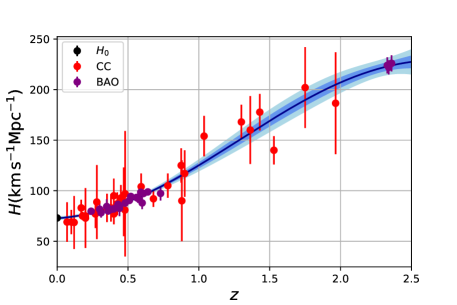
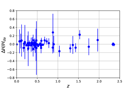
Figure 1: Upper graph: The reconstructed behavior of $H(z)$, arising from the 31 CC data points, the 23 BAO data points of radial method, and with $H_{0}=73.04\pm 1.04km\ s^{-1}Mpc^{-1}$. The dark curve denotes the mean value, while the blue and light blur shaded areas mark the allowed regions at $1\sigma$ and $2\sigma$ confidence level respectively. Lower graph: The corresponding residuals quantified by the quantity $\Delta H/{H_{da}}$, where $\Delta H=H_{da}-H_{re}$ represents the Hubble parameter difference between the observational value $H_{da}$ and the reconstructed value $H_{re}$.

3.3 Reconstruction in the Case of $f(T)$ Cosmology

In the previous subsection we reconstructed in a model-independent way the Hubble function. Hence, we can now use the obtained form in order to reconstruct the $f(T)$ function itself that is responsible for producing it. Since the torsion scalar in FLRW geometry is only a function of the Hubble function and not of its derivative, the whole procedure is significantly easier than in other modified gravity theories, such as $f(R)$ gravity.

The modified Friedmann equation (8) provides the relation between the $f(T)$ function and $H(z)$. For small $\Delta z$ we can use the approximation

$$f_{T}\equiv\frac{df(T)}{dT}=\frac{df/dz}{dT/dz}=\frac{f^{\prime}}{T^{\prime}},$$ (17)

with

$$f^{\prime}(z)\approx\frac{f(z+\Delta z)-f(z)}{\Delta z},$$ (18)

and thus $f_{T}$ can be represented by $f(z)$ and $H(z)$. Furthermore, we can extract the recursive relation between the consecutive redshifts ($z_{i}$ and $z_{i+1}$), namely writing $f(z_{i+1})$ as a function of $f\left(z_{i}\right)$, $H(z_{i})$ and $H^{\prime}\left(z_{i}\right)$ as (Cai et al., 2020; Briffa et al., 2020; Ren et al., 2021a)

$$\!\!\!\!\!\!\!\!\!\!\!\!\!\!f\left(z_{i+1}\right)=f\left(z_{i}\right)+6\left(z_{i+1}-z_{i}\right)\frac{H^{\prime}\left(z_{i}\right)}{H\left(z_{i}\right)}$$

$$\ \ \ \ \ \ \ \cdot\left[H^{2}\left(z_{i}\right)-H_{0}^{2}\Omega_{m0}\left(1+z_{i}\right)^{3}+\frac{f\left(z_{i}\right)}{6}\right].$$ (19)

From this expression we can obtain the value of $f$ at the redshift $z_{i+1}$, as long as we know the parameters at the redshift $z_{i}$. Finally, from the relation between $T$ and $H$, and the evolution of $H(z)$, we can directly extract the expression of $f$ as a function of $T$.

4 Results and features of the reconstructed forms

In this section we apply the above procedure and we extract the specific $f(T)$ form, investigating its features.

4.1 Reconstruction Considering Special Function Terms

With the model-independent reconstruction method introduced in Section 3, we can reconstruct $f(T)$ by fitting $H(z)$ and $H^{\prime}(z)$. As we described, the observational Hubble data directly determine $H(z)$, and thus by applying the Gaussian processes we reconstruct $H^{\prime}(z)$ too. Hence, we can finally use Eq. (19) and reconstruct the corresponding $f(T)$ form with $\Omega_{m0}=0.3$ presented in Fig. 2, where $T_{0}$ is the value of $T$ at present. When $f(T)=-2\Lambda_{c}$ we recover $\Lambda$CDM cosmology. Note that the units of both $T$ and $f(T)$ are $(\mathrm{km}\,\mathrm{s}^{-1}\mathrm{Mpc}^{-1})^{2}$.

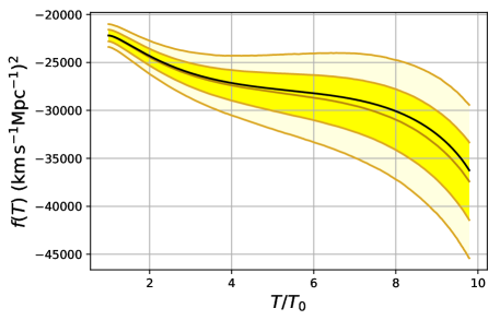
Figure 2: The reconstructed $f(T)$ function from observational Hubble data through Gaussian processes. The yellow and light yellow areas mark the regions of $1\sigma$ and $2\sigma$ confidence level respectively, while the black curve arises using the best-fit curve of $f(T)$. Both $T$ and $f(T)$ are measured in units of $(\mathrm{km}\,\mathrm{s}^{-1}\mathrm{Mpc}^{-1})^{2}$ and $T_{0}=-6H_{0}^{2}$.

Nevertheless, let us note here that the reconstructed $f(T)$ form in Fig. 2 is not the only function that can provide the corresponding evolution of $H(z)$ of Fig. 1, since as we mentioned above the addition of the special term $\sqrt{T/T_{0}}$ will not affect the evolution at the background level. Thus, for any $f_{re}(T)$ form that is reconstructed using the Gaussian processes, there is an extra possibility, namely a more general $f_{ge}(T)=f_{re}(T)+C\sqrt{T/T_{0}}$, where $C$ is an arbitrary coefficient, that will produce the same evolution of $H(z)$. This behavior is depicted in Fig. 3, where the different $f(T)$ forms correspond to the same background evolution of the universe.

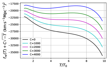
Figure 3: The reconstructed general $f(T)$ function $f_{ge}(T)=f_{re}(T)+C\sqrt{T/T_{0}}$, with $f_{re}(T)$ the reconstructed mean curve of Fig. 2, with $T_{0}=-6H_{0}^{2}$ and different choices of the parameter $C$. Both $T$ and $f(T)$, as well as $C$, are measured in units of $(\mathrm{km}\,\mathrm{s}^{-1}\mathrm{Mpc}^{-1})^{2}$.

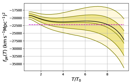
Figure 4: The reconstructed general $f(T)$ function $f_{ge}(T)=f_{re}(T)+C\sqrt{T/T_{0}}$, with $f_{re}(T)$ the reconstructed result of Fig. 2, in the specific case where $C=2927$ compared to the $\Lambda$CDM model (red dotted line). The latter lies within the $1\sigma$ reconstructed region for a relatively large time range. Both $T$ and $f(T)$, as well as $C$, are measured in units of $(\mathrm{km}\,\mathrm{s}^{-1}\mathrm{Mpc}^{-1})^{2}$ and $T_{0}=-6H_{0}^{2}$.

We can now use the above features in order to extract the reconstructed function that is closest to the $\Lambda$CDM cosmology bust still be in agreement with the data. As we show in Fig. 4, applying the curve fitting method we find that when the coefficient is $C=2927$ the reconstructed function is closest to the cosmological constant, or equivalently in this case the cosmological constant lies within the $1\sigma$ region of the reconstructed $f(T)$ model for a relatively large time range.

4.2 Analytic Fittings of the Reconstructed Function

In order to describe the reconstructed $f(T)$ function and its corresponding cosmological parameters in a more accurate way, we use polynomial fittings to extract analytic forms. The function fitting is based on the 251 reconstructed $f(T)$ points, while the original data source contains $H(z)$. Through Gaussian processes and approximate reconstruction, we can transform the information of $H(z)$ into the evolution of $f(T)$, and thus we can find the appropriate analytical expression of $f(T)$. In order to quantify the efficiency of the fitting of the various models, we need to implement particular information criteria.

The Bayesian Information Criterion (BIC) is the Criterion to select the model with the best fitting behavior among many models, and the model with the lower BIC is statistically favored (Liddle, 2007; Anagnostopoulos et al., 2019). BIC is defined as

$$\mathrm{BIC}=-2\ln\left(\mathcal{L}_{\max}\right)+k\ln\left(N_{\text{tot }}\right),$$ (20)

where $\mathcal{L}_{\max}$ is the maximized value of the likelihood function of the specific model, $N_{\text{tot }}$ is the number of data points, and $k$ the number of the model parameters. In Tab.1 we summarize the BIC values of the standard model $f(T)=-2\Lambda+a_{0}\sqrt{T/T_{0}}+a_{1}T$, the best fit quadratic polynomial $f(T)$ model $f(T)=-2\Lambda+a_{0}\sqrt{T/T_{0}}+a_{1}T+a_{2}T^{2}$, the best fit cubic polynomial $f(T)$ model $f(T)=-2\Lambda+a_{0}\sqrt{T/T_{0}}+a_{1}T+a_{2}T^{2}+a_{3}T^{3}$, as well as the best fit quartic polynomial $f(T)$ model $f(T)=-2\Lambda+a_{0}\sqrt{T/T_{0}}+a_{1}T+a_{2}T^{2}+a_{3}T^{3}+a_{4}T^{4}$, compared to the reconstructed result. Since the parameter $a_{0}$ does not affect the evolution of $H(z)$, and $a_{1}$ can be eliminated by parameter rescaling, these two parameters are not effective degrees of freedom. Standard model and quadratic polynomial model are not efficient to quantify the reconstructed $f(T)$ functions. On the other hand, quartic polynomial describes the reconstructed functions well, nevertheless the extra parameters cause its BIC to be less good than cubic polynomial. As we deduce from BIC, the cubic polynomial $f(T)$ is the best fitting model.

Model	$BIC$	$\Delta BIC$
$\Lambda$CDM	42.54	14.49
quadratic polynomial $f(T)$ model	37.28	9.23
cubic polynomial $f(T)$ model	28.05	0
quartic polynomial $f(T)$ model	33.57	5.52

Table 1: The BIC values for the examined $f(T)$ models, alongside the corresponding differences $\Delta BIC=BIC-BIC_{min}$.

In summary, we chose cubic polynomials, including the mentioned square-root term $\sqrt{T/T_{0}}$, to describe the reconstructed $f(T)$ function analytically, namely:

$$f(T)=-2\Lambda+a_{0}\sqrt{T/T_{0}}+a_{1}T+a_{2}T^{2}+a_{3}T^{3},$$ (21)

and the fitting result is depicted in Fig. 5. The analytic function (dashed green curve) can describe the model-independent reconstructed $f(T)$ form (red curve) very efficiently by choosing $a_{3}=-93.50$, $a_{2}=1750$, $a_{1}=-15650$, $a_{0}=21570$ and $\Lambda=14850$ in units of $(\mathrm{km}\,\mathrm{s}^{-1}\mathrm{Mpc}^{-1})^{2}$ .

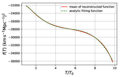
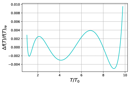
Figure 5: Upper graph: The best fit analytical model of $f(T)$ gravity (dashed purple curve), namely $f(T)=-2\Lambda+a_{0}\sqrt{T/T_{0}}+a_{1}T+a_{2}T^{2}+a_{3}T^{3}$, with $a_{3}=-93.50$, $a_{2}=1750$, $a_{1}=-15650$, $a_{0}=21570$ and $\Lambda=14850$ in units of $(\mathrm{km}\,\mathrm{s}^{-1}\mathrm{Mpc}^{-1})^{2}$, and the mean curve of the model-independent reconstructed $f(T)$ from OHD (orange curve). Lower graph: The corresponding differences quantified by the quantity $\Delta f(T)/{f(T)_{re}}$, where $\Delta H=f(T)_{re}-f(T)_{th}$ represents the Hubble parameter difference between the reconstructed value $f(T)_{re}$ and the analytical value $f(T)_{th}$.

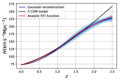
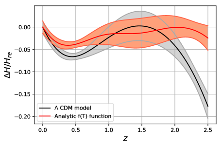
Figure 6: Upper graph: The $H(z)$ evolution obtained from the Gaussian process reconstruction (blue curves and shadows), from the analytical expression (21) (red curve), and from $\Lambda$CDM scenario (black curve). Lower graph: The corresponding differences quantified by the quantity $\Delta H/{H_{re}}$, where $\Delta H=H_{re}-H_{th}$ represents the Hubble parameter difference between the reconstructed value $H_{re}$ and the theoretical value $H_{th}$.

As a cross-test of the above procedure we proceed as follows. Since we have obtained the fittings of the analytic expression of the $f(T)$ function, we can insert Eq. (21) into the modified Friedmann equation (8) and extract the solution for $H(z)$. In the upper graph of Fig. 6 we present the results, namely the $H(z)$ obtained from the Gaussian process reconstruction and the $H(z)$ obtained from the analytical expression (21), and for completeness we add also the $H(z)$ corresponding to $\Lambda$CDM cosmology. Additionally, in order to examine the corresponding differences we introduce the quantity $\Delta H/{H_{re}}$, where $\Delta H=H_{re}-H_{th}$ represents the Hubble parameter difference between the reconstructed value $H_{re}$ and the theoretical value $H_{th}$. In the the lower graph of Fig. 6 we present its behavior, and as we can see, compared to $\Lambda$CDM model the analytical form (21) produces a result closer to that of data reconstruction.

5 Conclusion and Discussions

In this work we considered the effective field theory of $f(T)$ gravity as a framework to study the background evolution of the universe. We used the latest observational Hubble data and the $H_{0}$ measurement, and we reconstructed the Hubble function $H(z)$ by applying Gaussian processes. Then we used the obtained form in order to reconstruct the $f(T)$ function in a model-independent way. Since the special term $\sqrt{T/T_{0}}$ does not affect the evolution of the cosmological background, the family of all functions $f_{ge}(T)=f_{re}(T)+C\sqrt{T/T_{0}}$ produces the same background evolution with the reconstructed $f_{re}(T)$ form.

Having the $f(T)$ form obtained from data reconstruction, we performed a fitting by using polynomial functions containing additionally the square root term. We found that the reconstructed $f(T)$ expression presented in Eq. (21) may describe observations more efficiently than the $\Lambda$CDM scenario. This is the main result of the present work.

Furthermore, we expressed the Friedmann equations under $f(T)$ gravity as the recursive expression of $f(z)$, applying different approximation methods. This can be well combined with the $H(z)$ obtained through the Gaussian processes, in order to obtain the reconstruction of $f(T)$ function. We mention here that there are alternative procedures to reconstruct the $f(T)$ function. Specifically, the redshift $z$ can be expressed in terms of Hubble, deceleration, jerk and snap parameters, through the back scattering approach. Combined with a general function that sets $f$ to $z$, the reconstruction of $f(T)$ can be achieved (Capozziello et al., 2017). This reconstruction method is suitable when we have information at $z=0$. Moreover, it is an effective method to use other polynomials to approximate $f(z)$ and perform parameter fittings (Capozziello et al., 2019). Using suitable polynomials can achieve the same effect as the $f(z)$ recursive expressions of the present work.

Finally, we mention that the above analysis was based on data by HST and SH0ES teams, however since the tension between different datasets increases (Riess et al., 2021), it would be interesting to extend it using the Pantheon$+$ Type Ia supernovae (SNIa) data (Brout et al., 2022; Scolnic et al., 2021; Brownsberger et al., 2021). Additionally, as mentioned above, the $a_{0}\sqrt{T/T_{0}}$ term does not affect the background cosmological evolution, however at the perturbative level, and in particular at the evolution equation of the matter overdensity, this term will have an effect since different $a_{0}$ values will lead to different gravitational constant $G_{\text{eff}}={G_{N}}/{(1+f_{T})}$ (Anagnostopoulos et al., 2019). Hence, although this term does not affect the cosmological background, and hence the Gaussian processes procedure, it does affect the evolution of perturbations. In summary, it would be both interesting and necessary to perform the Gaussian process analysis using additionally SNIa as well as growth data, in order to obtain more accurate results and break the degeneracies between different $f(T)$ forms. Since these investigations lie beyond the scope of the present work, are left for future projects.

References

- Abdalla et al. (2022) Abdalla, E., et al. 2022, JHEAp, 34, 49, doi: 10.1016/j.jheap.2022.04.002
- Addazi et al. (2022) Addazi, A., et al. 2022, Prog. Part. Nucl. Phys., 125, 103948, doi: 10.1016/j.ppnp.2022.103948
- Aghanim et al. (2020) Aghanim, N., et al. 2020, Astron. Astrophys., 641, A6, doi: 10.1051/0004-6361/201833910
- Aldrovandi & Pereira (2013) Aldrovandi, R., & Pereira, J. G. 2013, Teleparallel Gravity: An Introduction, Vol. 173 (Springer), doi: 10.1007/978-94-007-5143-9
- Alestas et al. (2022) Alestas, G., Perivolaropoulos, L., & Tanidis, K. 2022. https://arxiv.org/abs/2201.05846
- Aljaf et al. (2021) Aljaf, M., Gregoris, D., & Khurshudyan, M. 2021, Eur. Phys. J. C, 81, 544, doi: 10.1140/epjc/s10052-021-09306-2
- Anagnostopoulos et al. (2019) Anagnostopoulos, F. K., Basilakos, S., & Saridakis, E. N. 2019, Phys. Rev. D, 100, 083517, doi: 10.1103/PhysRevD.100.083517
- Arkani-Hamed et al. (2007) Arkani-Hamed, N., Dubovsky, S., Nicolis, A., Trincherini, E., & Villadoro, G. 2007, JHEP, 05, 055, doi: 10.1088/1126-6708/2007/05/055
- Bahamonde et al. (2015) Bahamonde, S., Böhmer, C. G., & Wright, M. 2015, Phys. Rev. D, 92, 104042, doi: 10.1103/PhysRevD.92.104042
- Bahamonde et al. (2020) Bahamonde, S., Dialektopoulos, K. F., Hohmann, M., & Levi Said, J. 2020, Class. Quant. Grav., 38, 025006, doi: 10.1088/1361-6382/abc441
- Bahamonde et al. (2022) Bahamonde, S., Dialektopoulos, K. F., Hohmann, M., et al. 2022. https://arxiv.org/abs/2203.00619
- Bahamonde et al. (2019) Bahamonde, S., Flathmann, K., & Pfeifer, C. 2019, Phys. Rev. D, 100, 084064, doi: 10.1103/PhysRevD.100.084064
- Bahamonde et al. (2021) Bahamonde, S., Dialektopoulos, K. F., Escamilla-Rivera, C., et al. 2021. https://arxiv.org/abs/2106.13793
- Ballardini & Finelli (2021) Ballardini, M., & Finelli, F. 2021. https://arxiv.org/abs/2112.15126
- Benevento et al. (2020) Benevento, G., Hu, W., & Raveri, M. 2020, Phys. Rev. D, 101, 103517, doi: 10.1103/PhysRevD.101.103517
- Benisty (2021) Benisty, D. 2021, Phys. Dark Univ., 31, 100766, doi: 10.1016/j.dark.2020.100766
- Benisty et al. (2022) Benisty, D., Mifsud, J., Said, J. L., & Staicova, D. 2022. https://arxiv.org/abs/2202.04677
- Bernardo & Levi Said (2021) Bernardo, R. C., & Levi Said, J. 2021, JCAP, 09, 014, doi: 10.1088/1475-7516/2021/09/014
- Bloomfield et al. (2013) Bloomfield, J. K., Flanagan, E. E., Park, M., & Watson, S. 2013, JCAP, 08, 010, doi: 10.1088/1475-7516/2013/08/010
- Briffa et al. (2020) Briffa, R., Capozziello, S., Levi Said, J., Mifsud, J., & Saridakis, E. N. 2020, Class. Quant. Grav., 38, 055007, doi: 10.1088/1361-6382/abd4f5
- Brout et al. (2022) Brout, D., et al. 2022. https://arxiv.org/abs/2202.04077
- Brownsberger et al. (2021) Brownsberger, S., Brout, D., Scolnic, D., Stubbs, C. W., & Riess, A. G. 2021. https://arxiv.org/abs/2110.03486
- Cai et al. (2022) Cai, R.-G., Guo, Z.-K., Wang, S.-J., Yu, W.-W., & Zhou, Y. 2022. https://arxiv.org/abs/2202.12214
- Cai et al. (2016a) Cai, R.-G., Guo, Z.-K., & Yang, T. 2016a, Phys. Rev. D, 93, 043517, doi: 10.1103/PhysRevD.93.043517
- Cai et al. (2016b) Cai, Y.-F., Capozziello, S., De Laurentis, M., & Saridakis, E. N. 2016b, Rept. Prog. Phys., 79, 106901, doi: 10.1088/0034-4885/79/10/106901
- Cai et al. (2011) Cai, Y.-F., Chen, S.-H., Dent, J. B., Dutta, S., & Saridakis, E. N. 2011, Class. Quant. Grav., 28, 215011, doi: 10.1088/0264-9381/28/21/215011
- Cai et al. (2020) Cai, Y.-F., Khurshudyan, M., & Saridakis, E. N. 2020, Astrophys. J., 888, 62, doi: 10.3847/1538-4357/ab5a7f
- Cai et al. (2018) Cai, Y.-F., Li, C., Saridakis, E. N., & Xue, L. 2018, Phys. Rev. D, 97, 103513, doi: 10.1103/PhysRevD.97.103513
- Capozziello et al. (2011) Capozziello, S., Cardone, V. F., Farajollahi, H., & Ravanpak, A. 2011, Phys. Rev. D, 84, 043527, doi: 10.1103/PhysRevD.84.043527
- Capozziello et al. (2017) Capozziello, S., D’Agostino, R., & Luongo, O. 2017, Gen. Rel. Grav., 49, 141, doi: 10.1007/s10714-017-2304-x
- Capozziello et al. (2019) —. 2019, Int. J. Mod. Phys. D, 28, 1930016, doi: 10.1142/S0218271819300167
- Chen et al. (2011) Chen, S.-H., Dent, J. B., Dutta, S., & Saridakis, E. N. 2011, Phys. Rev. D, 83, 023508, doi: 10.1103/PhysRevD.83.023508
- Chen et al. (2020) Chen, Z., Luo, W., Cai, Y.-F., & Saridakis, E. N. 2020, Phys. Rev. D, 102, 104044, doi: 10.1103/PhysRevD.102.104044
- Cheung et al. (2008) Cheung, C., Creminelli, P., Fitzpatrick, A. L., Kaplan, J., & Senatore, L. 2008, JHEP, 03, 014, doi: 10.1088/1126-6708/2008/03/014
- Dainotti et al. (2021) Dainotti, M. G., De Simone, B., Schiavone, T., et al. 2021, Astrophys. J., 912, 150, doi: 10.3847/1538-4357/abeb73
- Dainotti et al. (2022) —. 2022, Galaxies, 10, 24, doi: 10.3390/galaxies10010024
- De Andrade et al. (2000) De Andrade, V., Guillen, L., & Pereira, J. 2000, in Teleparallel gravity: An Overview. https://arxiv.org/abs/gr-qc/0011087
- De Felice & Tsujikawa (2010) De Felice, A., & Tsujikawa, S. 2010, Living Rev. Rel., 13, 3, doi: 10.12942/lrr-2010-3
- Desmond et al. (2019) Desmond, H., Jain, B., & Sakstein, J. 2019, Phys. Rev. D, 100, 043537, doi: 10.1103/PhysRevD.100.043537
- Di Valentino et al. (2018) Di Valentino, E., Bøehm, C., Hivon, E., & Bouchet, F. R. 2018, Phys. Rev. D, 97, 043513, doi: 10.1103/PhysRevD.97.043513
- Di Valentino et al. (2015) Di Valentino, E., Melchiorri, A., & Silk, J. 2015, Phys. Rev. D, 92, 121302, doi: 10.1103/PhysRevD.92.121302
- Di Valentino et al. (2021a) Di Valentino, E., et al. 2021a, Astropart. Phys., 131, 102605, doi: 10.1016/j.astropartphys.2021.102605
- Di Valentino et al. (2021b) Di Valentino, E., Mena, O., Pan, S., et al. 2021b, Class. Quant. Grav., 38, 153001, doi: 10.1088/1361-6382/ac086d
- Draper & Smith (1998) Draper, N. R., & Smith, H. 1998, Applied regression analysis, Vol. 326 (John Wiley & Sons)
- Duchaniya et al. (2022) Duchaniya, L. K., Lohakare, S. V., Mishra, B., & Tripathy, S. K. 2022, Eur. Phys. J. C, 82, 448, doi: 10.1140/epjc/s10052-022-10406-w
- Elizalde & Khurshudyan (2019) Elizalde, E., & Khurshudyan, M. 2019, Phys. Rev. D, 99, 103533, doi: 10.1103/PhysRevD.99.103533
- Elizalde et al. (2020) Elizalde, E., Khurshudyan, M., Odintsov, S. D., & Myrzakulov, R. 2020, Phys. Rev. D, 102, 123501, doi: 10.1103/PhysRevD.102.123501
- Farooq et al. (2017) Farooq, O., Madiyar, F. R., Crandall, S., & Ratra, B. 2017, Astrophys. J., 835, 26, doi: 10.3847/1538-4357/835/1/26
- Frusciante & Perenon (2020) Frusciante, N., & Perenon, L. 2020, Phys. Rept., 857, 1, doi: 10.1016/j.physrep.2020.02.004
- Gelmini et al. (2021) Gelmini, G. B., Kusenko, A., & Takhistov, V. 2021, JCAP, 06, 002, doi: 10.1088/1475-7516/2021/06/002
- Gleyzes et al. (2013) Gleyzes, J., Langlois, D., Piazza, F., & Vernizzi, F. 2013, JCAP, 08, 025, doi: 10.1088/1475-7516/2013/08/025
- Golovnev & Koivisto (2018) Golovnev, A., & Koivisto, T. 2018, JCAP, 11, 012, doi: 10.1088/1475-7516/2018/11/012
- Gong & Mylova (2022) Gong, J.-O., & Mylova, M. 2022. https://arxiv.org/abs/2202.13882
- Gubitosi et al. (2013) Gubitosi, G., Piazza, F., & Vernizzi, F. 2013, JCAP, 02, 032, doi: 10.1088/1475-7516/2013/02/032
- Hohmann et al. (2017) Hohmann, M., Jarv, L., & Ualikhanova, U. 2017, Phys. Rev. D, 96, 043508, doi: 10.1103/PhysRevD.96.043508
- Holsclaw et al. (2010) Holsclaw, T., Alam, U., Sanso, B., et al. 2010, Phys. Rev. Lett., 105, 241302, doi: 10.1103/PhysRevLett.105.241302
- Jesus et al. (2021) Jesus, J. F., Valentim, R., Escobal, A. A., Pereira, S. H., & Benndorf, D. 2021. https://arxiv.org/abs/2112.09722
- Jiménez et al. (2021) Jiménez, J. B., Golovnev, A., Koivisto, T., & Veermäe, H. 2021, Phys. Rev. D, 103, 024054, doi: 10.1103/PhysRevD.103.024054
- Jimenez & Loeb (2002) Jimenez, R., & Loeb, A. 2002, Astrophys. J., 573, 37, doi: 10.1086/340549
- Karwal & Kamionkowski (2016) Karwal, T., & Kamionkowski, M. 2016, Phys. Rev. D, 94, 103523, doi: 10.1103/PhysRevD.94.103523
- Krssak et al. (2019) Krssak, M., van den Hoogen, R., Pereira, J., Böhmer, C., & Coley, A. 2019, Class. Quant. Grav., 36, 183001, doi: 10.1088/1361-6382/ab2e1f
- Krššák & Saridakis (2016) Krššák, M., & Saridakis, E. N. 2016, Class. Quant. Grav., 33, 115009, doi: 10.1088/0264-9381/33/11/115009
- Lee et al. (2022) Lee, B.-H., Lee, W., Colgáin, E. O., Sheikh-Jabbari, M. M., & Thakur, S. 2022, JCAP, 04, 004, doi: 10.1088/1475-7516/2022/04/004
- Levi Said et al. (2021) Levi Said, J., Mifsud, J., Sultana, J., & Adami, K. Z. 2021, JCAP, 06, 015, doi: 10.1088/1475-7516/2021/06/015
- Li et al. (2018) Li, C., Cai, Y., Cai, Y.-F., & Saridakis, E. N. 2018, JCAP, 10, 001, doi: 10.1088/1475-7516/2018/10/001
- Li et al. (2021) Li, E.-K., Du, M., Zhou, Z.-H., Zhang, H., & Xu, L. 2021, Mon. Not. Roy. Astron. Soc., 501, 4452, doi: 10.1093/mnras/staa3894
- Li et al. (2022) Li, M., Li, Z., & Rao, H. 2022. https://arxiv.org/abs/2201.02357
- Li & Zhao (2022) Li, M., & Zhao, D. 2022, Phys. Lett. B, 827, 136968, doi: 10.1016/j.physletb.2022.136968
- Liddle (2007) Liddle, A. R. 2007, Mon. Not. Roy. Astron. Soc., 377, L74, doi: 10.1111/j.1745-3933.2007.00306.x
- Magana et al. (2018) Magana, J., Amante, M. H., Garcia-Aspeitia, M. A., & Motta, V. 2018, Mon. Not. Roy. Astron. Soc., 476, 1036, doi: 10.1093/mnras/sty260
- Mukherjee & Banerjee (2022) Mukherjee, P., & Banerjee, N. 2022, Phys. Dark Univ., 36, 100998, doi: 10.1016/j.dark.2022.100998
- Mylova et al. (2021) Mylova, M., Moschou, M., Afshordi, N., & Magueijo, J. a. 2021. https://arxiv.org/abs/2112.08179
- Nojiri & Odintsov (2011) Nojiri, S., & Odintsov, S. D. 2011, Phys. Rept., 505, 59, doi: 10.1016/j.physrep.2011.04.001
- Odintsov & Oikonomou (2022) Odintsov, S. D., & Oikonomou, V. K. 2022, EPL, 137, 39001, doi: 10.1209/0295-5075/ac52dc
- Pan et al. (2019) Pan, S., Yang, W., Singha, C., & Saridakis, E. N. 2019, Phys. Rev. D, 100, 083539, doi: 10.1103/PhysRevD.100.083539
- Pfeifer & Schuster (2021) Pfeifer, C., & Schuster, S. 2021, Universe, 7, 153, doi: 10.3390/universe7050153
- Reid et al. (2019) Reid, M. J., Pesce, D. W., & Riess, A. G. 2019, Astrophys. J. Lett., 886, L27, doi: 10.3847/2041-8213/ab552d
- Ren et al. (2021a) Ren, X., Wong, T. H. T., Cai, Y.-F., & Saridakis, E. N. 2021a, Phys. Dark Univ., 32, 100812, doi: 10.1016/j.dark.2021.100812
- Ren et al. (2021b) Ren, X., Zhao, Y., Saridakis, E. N., & Cai, Y.-F. 2021b, JCAP, 10, 062, doi: 10.1088/1475-7516/2021/10/062
- Riess et al. (1998) Riess, A. G., et al. 1998, Astron. J., 116, 1009, doi: 10.1086/300499
- Riess et al. (2018) —. 2018, Astrophys. J., 855, 136, doi: 10.3847/1538-4357/aaadb7
- Riess et al. (2021) —. 2021. https://arxiv.org/abs/2112.04510
- Rodrigues & Bengaly (2021) Rodrigues, G., & Bengaly, C. 2021. https://arxiv.org/abs/2112.01963
- Santos et al. (2021) Santos, F. B. M. d., Gonzalez, J. E., & Silva, R. 2021. https://arxiv.org/abs/2112.15249
- Saridakis et al. (2021) Saridakis, E. N., et al. 2021. https://arxiv.org/abs/2105.12582
- Scolnic et al. (2021) Scolnic, D., et al. 2021. https://arxiv.org/abs/2112.03863
- Seikel & Clarkson (2013) Seikel, M., & Clarkson, C. 2013. https://arxiv.org/abs/1311.6678
- Seikel et al. (2012) Seikel, M., Clarkson, C., & Smith, M. 2012, JCAP, 06, 036, doi: 10.1088/1475-7516/2012/06/036
- Sen et al. (2021) Sen, A. A., Adil, S. A., & Sen, S. 2021. https://arxiv.org/abs/2112.10641
- Shah et al. (2021) Shah, P., Lemos, P., & Lahav, O. 2021, Astron. Astrophys. Rev., 29, 9, doi: 10.1007/s00159-021-00137-4
- Theodoropoulos & Perivolaropoulos (2021) Theodoropoulos, A., & Perivolaropoulos, L. 2021, Universe, 7, 300, doi: 10.3390/universe7080300
- Unzicker & Case (2005) Unzicker, A., & Case, T. 2005. https://arxiv.org/abs/physics/0503046
- Vagnozzi (2020) Vagnozzi, S. 2020, Phys. Rev. D, 102, 023518, doi: 10.1103/PhysRevD.102.023518
- Vagnozzi (2021) —. 2021, Phys. Rev. D, 104, 063524, doi: 10.1103/PhysRevD.104.063524
- von Marttens et al. (2021) von Marttens, R., Gonzalez, J. E., Alcaniz, J., Marra, V., & Casarini, L. 2021, Phys. Rev. D, 104, 043515, doi: 10.1103/PhysRevD.104.043515
- Wang & Meng (2017) Wang, D., & Meng, X.-H. 2017, Phys. Rev. D, 95, 023508, doi: 10.1103/PhysRevD.95.023508
- Wong et al. (2020) Wong, K. C., et al. 2020, Mon. Not. Roy. Astron. Soc., 498, 1420, doi: 10.1093/mnras/stz3094
- Xu et al. (2018) Xu, B., Yu, H., & Wu, P. 2018, Astrophys. J., 855, 89, doi: 10.3847/1538-4357/aaad12
- Yan et al. (2020) Yan, S.-F., Zhang, P., Chen, J.-W., et al. 2020, Phys. Rev. D, 101, 121301, doi: 10.1103/PhysRevD.101.121301
- Yang et al. (2015) Yang, T., Guo, Z.-K., & Cai, R.-G. 2015, Phys. Rev. D, 91, 123533, doi: 10.1103/PhysRevD.91.123533
- Yang et al. (2018) Yang, W., Pan, S., Di Valentino, E., et al. 2018, JCAP, 09, 019, doi: 10.1088/1475-7516/2018/09/019
- Yang et al. (2019) Yang, W., Pan, S., Di Valentino, E., Saridakis, E. N., & Chakraborty, S. 2019, Phys. Rev. D, 99, 043543, doi: 10.1103/PhysRevD.99.043543
- Yu et al. (2018) Yu, H., Ratra, B., & Wang, F.-Y. 2018, Astrophys. J., 856, 3, doi: 10.3847/1538-4357/aab0a2
- Yuan et al. (2019) Yuan, W., Riess, A. G., Macri, L. M., Casertano, S., & Scolnic, D. 2019, Astrophys. J., 886, 61, doi: 10.3847/1538-4357/ab4bc9
- Zhang & Xia (2016) Zhang, M.-J., & Xia, J.-Q. 2016, JCAP, 12, 005, doi: 10.1088/1475-7516/2016/12/005
- Zhang & Zhang (2021) Zhang, Y., & Zhang, H. 2021, Eur. Phys. J. C, 81, 706, doi: 10.1140/epjc/s10052-021-09501-1
- Zhao et al. (2017) Zhao, G.-B., et al. 2017, Nature Astron., 1, 627, doi: 10.1038/s41550-017-0216-z