First-Order Objective-Function-Free Optimization Algorithms and Their Complexity

Abstract

A class of algorithms for unconstrained nonconvex optimization is considered where the value of the objective function is never computed. The class contains a deterministic version of the first-order Adagrad method typically used for minimization of noisy function, but also allows the use of second-order information when available. The rate of convergence of methods in the class is analyzed and is shown to be identical to that known for first-order optimization methods using both function and gradients values. The result is essentially sharp and improves on previously known complexity bounds (in the stochastic context) by Défossez et al. (2020) and Gratton et al. (2022). A new class of methods is designed, for which a slightly worse and essentially sharp complexity result holds. Limited numerical experiments show that the new methods’ performance may be comparable to that of standard steepest descent, despite using significantly less information, and that this performance is relatively insensitive to noise.

Keywords: First-order methods, objective-function-free optimization (OFFO), Adagrad, convergence bounds, evaluation complexity, second-order models.

1 Introduction

This paper is concerned with Objective-Function-Free Optimization (OFFO) algorithms, which we define as numerical optimization methods in which the value of the problem’s objective function is never calculated, although we obviously assume that it exists. This is clearly at variance with the large majority of available numerical optimization algorithms, where the objective function is typically evaluated at every iteration, and its value then used to assess progress towards a minimizer and (often) to enforce descent. Dispensing with this information is therefore challenging. As it turns out, first-order OFFO methods (i.e. OFFO methods only using gradients) already exist for some time and have proved popular and useful in fields such as machine learning or sparse optimization, thereby justifying our interest. Algorithms such Adagrad [12], RMSprop [27], Adam [20] or AMSgrad [26] have been proposed and analyzed, recent contributions being [10] and [30] where improved convergence bounds for such methods are discussed. We refer the reader to the interesting paper [10] for a more extensive historical perspective on the developement of convergence theory of these first-order OFFO algorithms.

We take here the point of view that, although methods such as Adagrad and Adam have been defined and used in the context of probabilistic inexact gradient evaluations (such as resulting from sampling in finite-sum problems), they may neverthless be of interest in a deterministic context (i.e. when gradients are computed exactly). Indeed, in addition to being one of the very few existing approaches to OFFO, their deterministic evaluation complexity analysis provides a very useful template for that of their probabilistic counterparts. In particular, lower complexity bounds for the deterministic case immediately apply to the stochastic one. The purpose of the present contribution is thus to explore the deterministic context, the probablistic approach (using linear models only) being covered in a companion paper [17].

Should one be interested in first-order deterministic objective-function-free optimization, another obvious alternative would be to minimize the norm of the gradient (in the least-squares sense or in some other norm) using a derivative-free algorithm. To the best of our knowledge, this approach has not been widely experimented, maybe because it has the drawback of not being biased towards minimizing the underlying objective function: standard DFO algorithms, such as trust-region or adaptive regularization methods using finite-difference approximations, make, in this context, no distinction between minimizers, maximizers and other first-orders points of the original problem. More importantly, convergence of the DFO minimizer would have to occur to a global minimum for the original gradient to approximately vanish. The evaluation complexity of this approach is nevertheless appealing under these strong assumptions, because it was proved in [4] (see also [15] and [6, Section 13.1]) that reaching an $\epsilon$-approximate first-order point (of the gradient’s norm) can be obtained in ${\cal O}(\epsilon^{-2}+|\log(\epsilon)|)$ evaluations. We will compare below this theoretical bound with the new OFFO complexity results obtained in this paper.

Contributions:

In this paper, we

1. interpret the deterministic counterpart of Adagrad as a first-order trust-region method and use this interpretation to extend it to potentially use second-order information,

2. provide, for this extended method, an essentially sharp global bound on the gradient’s norm as a function of the iteration counter, which is identical to that known for first-order optimization methods using both function and gradients values,

3. use the developed framework to define a further class of first-order OFFO methods, for which an essentially sharp complexity result is also provided,

4. present some numerical experiments indicating that OFFO methods may indeed be competitive with steepest descent in efficiency and reliability.

Note: When this paper was completed, the authors became aware of the paper [16], where an adaptive trust-region algorithm is proposed in which the objective function is not evaluated, with a global rate of convergence similar to that presented below. However, while this algorithm is also a member of the class we study here, it is motivated differently (no relation to Adagrad is mentioned in [16]) and involves very different theoretical arguments (in particular, the question of sharpness for the complexity bound is not considered).

The paper is organized as follows. Section 2 introduces the new “trust-region minded” class of algorithms ASTR1 and the global rate of convergence of a subclass containing the deterministic Adagrad method are studied in Section 3. Section 4 then introduces a new ASTR1 subclass and analyzes its global rate of convergence. Some numerical illlustration is provided in Section 5. Conclusions are finally outlined in Section 6.

2 A class of first-order minimization methods

We consider the problem

$$\min_{x\in\hbox{\footnotesize I\hskip-2.0ptR}^{n}}f(x)$$ (2.1)

where $f$ is a smooth function from $\hbox{I\hskip-2.0ptR}^{n}$ to IR. In particular, we will assume in what follows that

AS.1:

the objective function $f(x)$ is continuously differentiable;

AS.2:

its gradient $g(x)\stackrel{{\scriptstyle\rm def}}{{=}}\nabla_{x}^{1}f(x)$ is Lipschitz continuous with Lipschitz constant $L\geq 0$, that is

$$\|g(x)-g(y)\|\leq L\|x-y\|$$

for all $x,y\in\hbox{I\hskip-2.0ptR}^{n}$, where, unless otherwise specified, $\|\cdot\|=\|\cdot\|_{2}$ is the Euclidean norm;

AS.3:

there exists a constant $\kappa_{g}\geq 1$ such that, for all $x$, $\|g(x)\|_{\infty}\leq\kappa_{g}$;

AS.4:

there exists a constant $f_{\rm low}$ such that, for all $x$, $f(x)\geq f_{\rm low}$.

AS.1, AS.2 and AS.4 are standard for the complexity analysis of optimization methods seeking first-order critical points, AS.4 guaranteeing in particular that the problem is well-posed. AS.3 is common in the analysis of stochastic OFFO methods (see [28, 10, 30, 17], for instance).

The class of methods of interest here are iterative and generate a sequence of iterates $\{x_{k}\}_{k\geq 0}$. The move from an iterate to the next directly depends on the gradient at $x_{k}$ and algorithm-dependent scaling factors $\{w_{k}=w(x_{0},\ldots,x_{k})\}$ whose main purpose is to control the move’s magnitude. In our analysis, we will assume that

AS.5:

for each $i\in\{1,\ldots,n\}$ there exists a constant $\varsigma_{i}\in(0,1]$ such that, $w_{i,k}\geq\varsigma_{i}$ for all $k\geq 0$.

Since scaling factors are designed to control the length of the step, they are strongly reminiscent of the standard mechanism of the much studied trust-region optimization methods (see [8] for an extensive coverage and [29] for a more recent survey). In trust-region algorithms, a model of the objective function at an iterate $x_{k}$ is built, typically using a truncated Taylor series, and a step $s_{k}$ is chosen that minimizes this model with a trust-region, that is a region where the model is assumed to represent the true objective function sufficiently well. This region is a ball around the current iterate, whose radius is updated adaptively from iteration to iteration, based on the quality of the prediction of the objective function value at the trial point $x_{k}+s_{k}$. For methods using gradient only, the model is then chosen as the first two terms of the Taylor’s expansion of $f$ at the iterate $x_{k}$. Although, we are interested here in methods where the objective function’s value is not evaluated, and therefore cannot be used to accept/reject iterates and update the trust-region radius, a similar mechanism may be designed, this time involving the scaling factors $\{w_{k}\}$. The resulting algorithm, which we call ASTR1 (for Adaptively Scaled Trust Region using 1rst order information) is stated 2.

Algorithm 2.1: ASTR1
Step 0: Initialization. A starting point $x_{0}$ is given. Constants $\kappa_{\mbox{\tiny B}}\geq 1$ and $\tau\in(0,1]$ are also given. Set $k=0$. Step 1: Define the TR. Compute $g_{k}=g(x_{k})$ and define $$\Delta_{i,k}=\frac{|g_{i,k}|}{w_{i,k}}$$ (2.2) where $w_{k}=w(x_{0},\ldots,x_{k})$. Step 2: Hessian approximation. Select a symmetric Hessian approximation $B_{k}$ such that $$\|B_{k}\|\leq\kappa_{\mbox{\tiny B}}.$$ (2.3) Step 3: GCP. Compute a step $s_{k}$ such that $$|s_{i,k}|\leq\Delta_{i,k}\;\;\;\;(i\in\{1,\ldots,n\}),$$ (2.4) and $$g_{k}^{T}s_{k}+{\scriptstyle\frac{1}{2}}s_{k}^{T}B_{k}s_{k}\leq\tau\left(g_{k}^{T}s_{k}^{Q}+{\scriptstyle\frac{1}{2}}(s_{k}^{Q})^{T}B_{k}s_{k}^{Q}\right),$$ (2.5) where $$s_{i,k}^{L}=-{\rm sgn}(g_{i,k})\Delta_{i,k},$$ (2.6) $$s^{Q}_{k}=\gamma_{k}s_{k}^{L},$$ (2.7) with $$\gamma_{k}=\left\{\begin{array}[]{ll}\min\left[1,\frac{\displaystyle|g_{k}^{T}s_{k}^{L}|}{\displaystyle(s_{k}^{L})^{T}B_{k}s_{k}^{L}}\right]&\;\;\mbox{if }\;\;(s_{k}^{L})^{T}B_{k}s_{k}^{L}>0,\\ 1&\;\;\mbox{otherwise.}\end{array}\right.$$ (2.8) Step 4: New iterate. Define $$x_{k+1}=x_{k}+s_{k},$$ (2.9) increment $k$ by one and return to Step 1.

The algorithm description calls for some comments.

1. Observe that we allow the use of second-order information by effectively defining a quadratic model

   $$g_{k}^{T}s+{\scriptstyle\frac{1}{2}}s^{T}B_{k}s$$ (2.10)

   where $B_{k}$ can of course be chosen as the true second-derivative matrix of $f$ at $x_{k}$ (provided it remains bounded to satisfy (2.3)) or any approximation thereof. Choosing $B_{k}=0$ results in a purely first-order algorithm.

   The condition (2.3) on the Hessian approximations is quite weak, and allows in particular for a variety of quasi-Newton approaches, limited-memory or otherwise. In a finite-sum context, sampling bounded Hessians is also possible.

2. Conditions (2.5)–(2.8) define a “generalized Cauchy point”, much in the spirit of standard trust-region methodology (see [8, Section 6.3] for instance), where the quadratic model (2.10) is minimized in (2.8) along a good first-order direction ($s_{k}^{L}$) to obtain a “Cauchy step” $s_{k}^{Q}$. Any step $s_{k}$ can then be accepted provided it remains in the trust region (see (2.4)) and enforces a decrease in the quadratic model which is a least a fraction $\tau$ of that achieved at the Cauchy step (see (2.5)).

3. At variance with many existing trust-region algorithms, the radius $\Delta_{k}$ of the trust-region (2.2) is not recurred adaptively from iteration to iteration depending on how well the quadratic model predicts function values, but is directly defined as a scaled version of the local gradient. This is not without similarities with the trust-region method proposed by [13], which corresponds to a scaling factor equal to $\|g_{k}\|^{-1}$.

4. As stated, the ASTR1 algorithm does not include a termination rule, but such a rule can easily be introduced by terminating the algorithm in Step 1 if $\|g_{k}\|\leq\epsilon$, where $\epsilon>0$ is a user-defined first-order accuracy threshold.

The algorithm being defined, the first step of our analysis is to derive a fundamental property of objective-function decrease, valid for all choices of the scaling factors satisfying AS.5.

Lemma 2.1

Suppose that AS.1, AS.2 and AS.5 hold. Then we have that, for all $k\geq 0$, $$f(x_{0})-f(x_{k+1})\geq\sum_{j=0}^{k}\sum_{i=1}^{n}\frac{g_{i,j}^{2}}{2\kappa_{\mbox{\tiny B}}w_{i,j}}\left[\tau\varsigma_{\min}-\frac{\kappa_{\mbox{\tiny BBL}}}{w_{i,j}}\right]$$ (2.11) where $\varsigma_{\min}\stackrel{{\scriptstyle\rm def}}{{=}}\min_{i\in\{1,\ldots,n\}}\varsigma_{i}$ and $\kappa_{\mbox{\tiny BBL}}\stackrel{{\scriptstyle\rm def}}{{=}}\kappa_{\mbox{\tiny B}}(\kappa_{\mbox{\tiny B}}+L)$.

• Proof.    Using (2.6) and AS.5, we deduce that, for every $j\geq 0$,

  $$|g_{j}^{T}s_{j}^{L}|=\sum_{i=1}^{n}\frac{g_{i,j}^{2}}{w_{i,j}}=\sum_{i=1}^{n}\frac{w_{i,j}g_{i,j}^{2}}{w_{i,j}^{2}}\geq\sum_{i=1}^{n}\frac{\varsigma_{i}g_{i,j}^{2}}{w_{i,j}^{2}}\geq\varsigma_{\min}\|s_{j}^{L}\|^{2}.$$ (2.12)

  Suppose first that $(s_{j}^{L})^{T}B_{j}s_{j}^{L}>0$ and $\gamma_{j}<1$. Then, in view of (2.7), (2.8), (2.12) and (2.3),

  $$g_{j}^{T}s_{j}^{Q}+{\scriptstyle\frac{1}{2}}(s_{j}^{Q})^{T}B_{j}s_{j}^{Q}=\gamma_{j}g_{j}^{T}s_{j}^{L}+{\scriptstyle\frac{1}{2}}\gamma_{j}^{2}(s_{j}^{L})^{T}B_{j}s_{j}^{L}=-\frac{(g_{j}^{T}s_{j}^{L})^{2}}{2(s_{j}^{L})^{T}B_{j}s_{j}^{L}}\leq-\frac{\varsigma_{\min}|g_{j}^{T}s_{j}^{L}|}{2\kappa_{\mbox{\tiny B}}}.$$

  Combining this inequality with the first equality in (2.12) then gives that

  $$g_{j}^{T}s_{j}^{Q}+{\scriptstyle\frac{1}{2}}(s_{j}^{Q})^{T}B_{j}s_{j}^{Q}\leq-\frac{\varsigma_{\min}}{2\kappa_{\mbox{\tiny B}}}\sum_{i=1}^{n}\frac{g_{i,j}^{2}}{w_{i,j}}.$$ (2.13)

  Suppose now that $(s_{j}^{L})^{T}B_{j}s_{j}^{L}\leq 0$ or $\gamma_{j}=1$. Then, using (2.7), (2.13) and (2.6),

  $$g_{j}^{T}s_{j}^{Q}+{\scriptstyle\frac{1}{2}}(s_{j}^{Q})^{T}B_{j}s_{j}^{Q}=g_{j}^{T}s_{j}^{L}+{\scriptstyle\frac{1}{2}}(s_{j}^{L})^{T}B_{j}s_{j}^{L}\leq{\scriptstyle\frac{1}{2}}g_{j}^{T}s_{j}^{L}<0$$

  and (2.13) then again follows from the bound $\kappa_{\mbox{\tiny B}}\geq 1$. Successively using AS.1–AS.2, (2.5), (2.13), (2.3) and (2.2) then gives that, for $j\geq 0$,

  $$f(x_{j+1}) \leq f(x_{j})+g_{j}^{T}s_{j}+{\scriptstyle\frac{1}{2}}s_{j}^{T}B_{j}s_{j}-{\scriptstyle\frac{1}{2}}s_{j}^{T}B_{j}s_{j}+{\scriptstyle\frac{1}{2}}L\|s_{j}\|^{2}$$ (2.14)

  $$\leq f(x_{j})+\tau\left(g_{j}^{T}s_{j}^{Q}+{\scriptstyle\frac{1}{2}}(s_{j}^{Q})^{T}B_{j}s_{j}^{Q}\right)+{\scriptstyle\frac{1}{2}}(\kappa_{\mbox{\tiny B}}+L)\|s_{j}\|^{2}$$

  $$\leq f(x_{j})-\sum_{i=1}^{n}\frac{\tau\varsigma_{\min}g_{i,j}^{2}}{2\kappa_{\mbox{\tiny B}}w_{i,j}}+{\scriptstyle\frac{1}{2}}(\kappa_{\mbox{\tiny B}}+L)\sum_{i=1}^{n}\Delta_{i,j}^{2}$$

  $$\leq f(x_{j})-\sum_{i=1}^{n}\frac{\tau\varsigma_{\min}g_{i,j}^{2}}{2\kappa_{\mbox{\tiny B}}w_{i,j}}+{\scriptstyle\frac{1}{2}}(\kappa_{\mbox{\tiny B}}+L)\sum_{i=1}^{n}\frac{g_{i,j}^{2}}{w_{i,j}^{2}}$$

  Summing up this inequality for $j\in\{0,\ldots,k\}$ then yields (2.11). $\Box$

Armed with Lemma 2.1, we are now in position to specify particular choices of the scaling factors $w_{i,k}$ and derive the convergence properties of the resulting variants of ASTR1.

3 An Adagrad-like variant of ASTR1 using second-order models

We first consider a choice of scaling factors directly derived from the definition of the Adagrad algorithm [12]. For given $\varsigma\in(0,1]$, $\vartheta\in(0,1]$ and $\mu\in(0,1)$, define, for all $i\in\{1,\ldots,n\}$ and for all $k\geq 0$,

$$w_{i,k}\in\left[\sqrt{\vartheta}\,v_{i,k},v_{i,k}\right]\;\;\mbox{ where }\;\;v_{i,k}\stackrel{{\scriptstyle\rm def}}{{=}}\left(\varsigma+\sum_{\ell=0}^{k}g_{i,\ell}^{2}\right)^{\mu}.$$ (3.1)

The Adagrad scaling factors are recovered by $\mu={\scriptstyle\frac{1}{2}}$ and $\vartheta=1$, and ASTR1 with (3.1) and $B_{k}=0$ is then the standard (deterministic) Adagrad method. The $\vartheta$ parameter is introduced for felxibility, in particular allowing non-monotone scaling factors. Without loss of generality, we assume that $\kappa_{g}^{2}\geq g_{i,0}^{2}+\varsigma$ for $i\in\{1,\ldots,n\}$.

Before stating the global rate of convergence of the variant of ASTR1 using (3.1), we first prove a crucial lemma, partly inspired by [28, 10].

Lemma 3.1

Let $\{a_{k}\}_{k\geq 0}$ be a non-negative sequence, $\alpha>0$, $\xi>0$ and define, for each $k\geq 0$, $b_{k}=\sum_{j=0}^{k}a_{j}$. Then if $\alpha\neq 1$, $$\sum_{j=0}^{k}\frac{a_{j}}{(\xi+b_{j})^{\alpha}}\leq\frac{1}{(1-\alpha)}((\xi+b_{k})^{1-\alpha}-\xi^{1-\alpha}).$$ (3.2) Otherwise (i.e. if $\alpha=1$), $$\sum_{j=0}^{k}\frac{a_{j}}{(\xi+b_{j})}\leq\log\left(\frac{\xi+b_{k}}{\xi}\right).$$ (3.3)

• Proof.    Consider first the case where $\alpha\neq 1$ and note that $\frac{1}{(1-\alpha)}x^{1-\alpha}$ is then a non-decreasing and concave function on $(0,+\infty)$. Setting $b_{-1}=0$ and using these properties, we obtain that, for $j\geq 0$,

  $$\frac{a_{j}}{(\xi+b_{j})^{\alpha}} \leq\frac{1}{1-\alpha}\left((\xi+b_{j})^{1-\alpha}-(\xi+b_{j}-a_{j})^{1-\alpha}\right)$$

  $$\leq\frac{1}{1-\alpha}\left((\xi+b_{j})^{1-\alpha}-(\xi+b_{j-1})^{1-\alpha}\right).$$

  We then obtain (3.2) by summing this inequality for $j\in\{0,\ldots,k\}$.

  Suppose now that $\alpha=1$, we then use the concavity and non-decreasing character of the logarithm to derive that

  $$\frac{a_{j}}{(\xi+b_{j})^{\alpha}}=\frac{a_{j}}{(\xi+b_{j})}\leq\log(\xi+b_{j})-\log(\xi+b_{j}-a_{j})\leq\log(\xi+b_{j})-\log(\xi+b_{j-1}).$$

  The inequality (3.3) then again follows by summing for $j\in\{0,\ldots,k\}$. $\Box$

From (3.2), we also obtain that, for $\alpha<1$,

$$\sum_{j=0}^{k}\frac{a_{j}}{(\xi+b_{j})^{\alpha}}\leq\frac{1}{(1-\alpha)}(\xi+b_{k})^{1-\alpha}$$ (3.4)

while, for $\alpha>1$,

$$\sum_{j=0}^{k}\frac{a_{j}}{(\xi+b_{j})^{\alpha}}\leq\frac{\xi^{1-\alpha}}{(\alpha-1)}.$$ (3.5)

Note that both the numerator and the denominator of the right-hand side of (3.2) tend to zero when $\alpha$ tends to one. Applying l’Hospital rule, we then see that this right-hand side tends to the right-hand side of (3.3) and the bounds on $\sum_{j=0}^{k}a_{j}/(\xi+b_{j})^{\alpha}$ are therefore continuous at $\alpha=1$.

Theorem 3.2

Suppose that AS.1–AS.4 hold and that the ASTR1 algorithm is applied to problem (2.1) with its scaling given by (3.1). If we define $$\Gamma_{0}\stackrel{{\scriptstyle\rm def}}{{=}}f(x_{0})-f_{\rm low},\;\;\;\;\kappa_{1}\stackrel{{\scriptstyle\rm def}}{{=}}\frac{\kappa_{g}^{2\mu}\kappa_{\mbox{\tiny B}}}{\tau\varsigma^{\mu}\sqrt{\vartheta}}\;\;\mbox{ and }\;\;\kappa_{2}\stackrel{{\scriptstyle\rm def}}{{=}}\frac{n\kappa_{1}(\kappa_{\mbox{\tiny B}}+L)}{\vartheta},$$ then, (i) if $0<\mu<{\scriptstyle\frac{1}{2}}$, $$\operatorname*{average}_{j\in\{0,\ldots,k\}}\|g_{j}\|^{2}\leq\min\left[\frac{\kappa_{3}}{k+1},\;\frac{\kappa_{4}}{(k+1)^{1-\mu}}+\frac{\kappa_{5}}{(k+1)^{\mu}}\right]$$ (3.6) with $$\kappa_{3}=\max\left\{\varsigma,\left[\frac{4\,n\,\kappa_{\mbox{\tiny BBL}}}{(1-2\mu)\tau\varsigma^{\mu}\vartheta^{\scriptstyle\frac{3}{2}}}\right]^{\scriptstyle\frac{1}{\mu}},\left[\frac{2^{2\mu}\vartheta(1-2\mu)\Gamma_{0}}{n(\kappa_{\mbox{\tiny B}}+L)}\right]^{{\scriptstyle\frac{1}{1-2\mu}}}\right\},$$ (3.7) $$\kappa_{4}=2\kappa_{1}\Gamma_{0}\;\;\mbox{ and }\;\;\kappa_{5}=\left(\frac{\kappa_{2}}{1-2\mu}\right)\Big{[}(\varsigma+\kappa_{g}^{2})^{1-2\mu}-\varsigma^{1-2\mu}\Big{]};$$ (ii) if $\mu={\scriptstyle\frac{1}{2}}$, $$\operatorname*{average}_{j\in\{0,\ldots,k\}}\|g_{j}\|^{2}\leq\min\left[\frac{\kappa_{6}}{k+1},\frac{\kappa_{4}}{\sqrt{k+1}}+\kappa_{2}\,\frac{\log\big{(}1+(k+1)\varsigma^{-1}\kappa_{g}^{2}\big{)}}{\sqrt{k+1}}\right]$$ (3.8) with $$\kappa_{6}=\max\left\{\varsigma,\frac{\displaystyle 1}{\displaystyle 2}e^{\frac{2\Gamma_{0}\vartheta}{n(\kappa_{B}+L)}},\frac{1}{2}\left(\frac{8n\kappa_{\mbox{\tiny B}}(\kappa_{\mbox{\tiny B}}+L)}{\tau\sqrt{\varsigma}\vartheta^{\scriptstyle\frac{3}{2}}}\right)^{2}\,\left|W_{-1}\left(-\frac{\tau\sqrt{\varsigma}\vartheta^{\scriptstyle\frac{3}{2}}}{8n\kappa_{\mbox{\tiny B}}(\kappa_{\mbox{\tiny B}}+L)}\right)\right|^{2}\right\},$$ (3.9) where $W_{-1}$ is the second branch of the Lambert function [9]; (iii) if ${\scriptstyle\frac{1}{2}}<\mu<1$, $$\operatorname*{average}_{j\in\{0,\ldots,k\}}\|g_{j}\|^{2}\leq\min\left[\frac{\kappa_{7}}{k+1},\frac{\kappa_{8}}{(k+1)^{1-\mu}}\right]$$ (3.10) with $$\kappa_{7}\stackrel{{\scriptstyle\rm def}}{{=}}\!\left[\frac{2^{1+\mu}\kappa_{\mbox{\tiny B}}}{\tau\varsigma^{\mu}\sqrt{\vartheta}}\left(\!\Gamma_{0}+\frac{n(\kappa_{\mbox{\tiny B}}+L)\varsigma^{1-2\mu}}{2\vartheta(2\mu-1)}\right)\right]^{{\scriptstyle\frac{1}{1-\mu}}}\mbox{and}\;\;\;\;\kappa_{8}\stackrel{{\scriptstyle\rm def}}{{=}}2\kappa_{1}\Gamma_{0}+\!\left(\frac{\kappa_{2}\varsigma^{1-2\mu}}{2\mu-1}\right).$$ (3.11)

• Proof.    We see from (3.1) that $w_{i,k}$ verifies AS.5. We may thus use Lemma 2.1. Moreover, (3.1) and the fact that $\kappa_{g}^{2}\geq g_{i,0}^{2}+\varsigma$ for $i\in\{1,\ldots,n\}$ also imply that

  $$\varsigma^{\mu}\sqrt{\vartheta}\leq w_{i,j}\leq\min\left[\,\kappa_{g}^{2\mu}(j+1)^{\mu},\left(\varsigma+\sum_{\ell=0}^{j}\|g_{\ell}\|^{2}\right)^{\mu}\,\right]$$ (3.12)

  for all $j\geq 0$ and all $i\in\{1,\ldots,n\}$. We now deduce from (2.2) and (2.11) that, for $k\geq 0$,

  $$\begin{array}[]{lcl}f(x_{k+1})&\leq&f(x_{0})-\displaystyle\sum_{j=0}^{k}\frac{\displaystyle\tau\varsigma^{\mu}\sqrt{\vartheta}\,\|g_{j}\|^{2}}{\displaystyle 2\kappa_{\mbox{\tiny B}}\max_{i\in\{1,\ldots,n\}}w_{i,k}}+{\scriptstyle\frac{1}{2}}(\kappa_{\mbox{\tiny B}}+L)\displaystyle\sum_{i=1}^{n}\displaystyle\sum_{j=0}^{k}\Delta_{i,j}^{2}.\end{array}$$ (3.13)

  For each $i\in\{1,\ldots,n\}$, we then apply Lemma 3.1 with $a_{\ell}=g_{i,\ell}^{2}$, $\xi=\varsigma$ and $\alpha=2\mu<1$, and obtain from (2.2) and (3.1) that,

  $$\sum_{j=0}^{k}\Delta_{i,j}^{2}\leq\frac{\displaystyle 1}{\displaystyle\vartheta(1-2\mu)}\left[\left(\varsigma+\displaystyle\sum_{\ell=0}^{k}g_{i,\ell}^{2}\right)^{1-2\mu}-\varsigma^{1-2\mu}\right]\leq\frac{\displaystyle 1}{\displaystyle\vartheta(1-2\mu)}\left(\varsigma+\displaystyle\sum_{\ell=0}^{k}g_{i,\ell}^{2}\right)^{1-2\mu}.$$ (3.14)

  Now

  $$\sum_{i=1}^{n}\displaystyle\sum_{j=0}^{k}\Delta_{i,j}^{2}\leq\displaystyle\sum_{i=1}^{n}\frac{\displaystyle 1}{\displaystyle\vartheta(1-2\mu)}\left(\varsigma+\displaystyle\sum_{i=1}^{n}\displaystyle\sum_{\ell=0}^{k}g_{i,\ell}^{2}\right)^{1-2\mu}\leq\frac{\displaystyle n}{\displaystyle\vartheta(1-2\mu)}\left(\varsigma+\displaystyle\sum_{\ell=0}^{k}\|g_{\ell}\|^{2}\right)^{1-2\mu}$$ (3.15)

  and thus substituting this bound in (3.13) and using AS.4 gives that

  $$\sum_{j=0}^{k}\frac{\displaystyle\tau\varsigma^{\mu}\sqrt{\vartheta}\|g_{j}\|^{2}}{\displaystyle 2\kappa_{\mbox{\tiny B}}\max_{i\in\{1,\ldots,n\}}w_{i,k}}\leq\Gamma_{0}+\frac{n(\kappa_{\mbox{\tiny B}}+L)}{2\vartheta}(1-2\mu)\left(\varsigma+\sum_{j=0}^{k}\|g_{j}\|^{2}\right)^{1-2\mu}.$$ (3.16)

  Suppose now that

  $$\sum_{j=0}^{k}\|g_{j}\|^{2}\geq\max\left\{\varsigma,\left[\frac{2^{2\mu}\vartheta(1-2\mu)\Gamma_{0}}{n(\kappa_{\mbox{\tiny B}}+L)}\right]^{{\scriptstyle\frac{1}{1-2\mu}}}\right\},$$ (3.17)

  implying

  $$\varsigma+\sum_{j=0}^{k}\|g_{j}\|^{2}\leq 2\sum_{j=0}^{k}\|g_{j}\|^{2}\;\;\mbox{and}\;\;\Gamma_{0}\leq\frac{n(\kappa_{\mbox{\tiny B}}+L)}{2\vartheta(1-2\mu)}\left(2\sum_{j=0}^{k}\|g_{j}\|^{2}\right)^{1-2\mu}.$$

  Then, using (3.16) and (3.12),

  $$\frac{\tau\varsigma^{\mu}\sqrt{\vartheta}}{2^{1+\mu}\,\kappa_{\mbox{\tiny B}}\left[\sum_{\ell=0}^{k}\|g_{\ell}\|^{2}\right]^{\mu}}\sum_{j=0}^{k}\|g_{j}\|^{2}\leq\frac{2^{1-2\mu}\,n\,(\kappa_{\mbox{\tiny B}}+L)}{\vartheta}(1-2\mu)\left(\sum_{j=0}^{k}\|g_{j}\|^{2}\right)^{1-2\mu}.$$

  Solving this inequality for $\sum_{j=0}^{k}\|g_{j}\|^{2}$ gives that

  $$\sum_{j=0}^{k}\|g_{j}\|^{2}\leq\left[\frac{4\,n\,\,\kappa_{\mbox{\tiny BBL}}}{(1-2\mu)\tau\varsigma^{\mu}\vartheta^{\scriptstyle\frac{3}{2}}}\right]^{{\scriptstyle\frac{1}{\mu}}}$$

  and therefore

  $$\operatorname*{average}_{j\in\{0,\ldots,k\}}\|g_{j}\|^{2}\leq\left[\frac{4\,n\,\kappa_{\mbox{\tiny BBL}}}{(1-2\mu)\tau\varsigma^{\mu}\vartheta^{\scriptstyle\frac{3}{2}}}\right]^{{\scriptstyle\frac{1}{\mu}}}\cdot\frac{1}{{k+1}}.$$ (3.18)

  Alternatively, if (3.17) fails, then

  $$\operatorname*{average}_{j\in\{0,\ldots,k\}}\|g_{j}\|^{2}<\max\left\{\varsigma,\left[\frac{2^{2\mu}\vartheta(1-2\mu)\Gamma_{0}}{n(\kappa_{\mbox{\tiny B}}+L)}\right]^{{\scriptstyle\frac{1}{1-2\mu}}}\right\}\cdot\frac{1}{k+1}.$$ (3.19)

  We may also use AS.4 after substituting (3.14) in (3.13) and using (3.12) to deduce that

  $$\sum_{j=0}^{k}\frac{\displaystyle\tau\varsigma^{\mu}\sqrt{\vartheta}\|g_{j}\|^{2}}{\displaystyle 2\kappa_{g}^{2\mu}\kappa_{\mbox{\tiny B}}(k+1)^{\mu}}\leq\Gamma_{0}+\frac{n(\kappa_{\mbox{\tiny B}}+L)}{2\vartheta(1-2\mu)}\left[\big{(}\varsigma+\kappa_{g}^{2}(k+1)\big{)}^{1-2\mu}-\varsigma^{1-2\mu}\right]$$

  and therefore that

  $$\begin{array}[]{l}\displaystyle\operatorname*{average}_{j\in\{0,\ldots,k\}}\|g_{j}\|^{2}\\[8.61108pt] \hskip 14.22636pt\leq\frac{\displaystyle 2\kappa_{g}^{2\mu}\kappa_{\mbox{\tiny B}}}{\displaystyle\tau\varsigma^{\mu}\sqrt{\vartheta}(k+1)^{1-\mu}}\left[\Gamma_{0}+\frac{\displaystyle n(\kappa_{\mbox{\tiny B}}+L)}{\displaystyle 2\vartheta(1-2\mu)}(k+1)^{1-2\mu}\left((\varsigma+\kappa_{g}^{2})^{1-2\mu}\right)-\varsigma^{1-2\mu}\right].\end{array}$$ (3.20)

  Combining (3.18), (3.19) and (3.20) gives (3.6).

  Let us now consider the case where $\mu={\scriptstyle\frac{1}{2}}$. For each $i\in\{1,\ldots,n\}$, we apply Lemma 3.1 with $a_{k}=g_{i,k}^{2}$, $\xi=\varsigma$ and $\alpha=2\mu=1$ and obtain that,

  $$\sum_{i=1}^{n}\displaystyle\sum_{j=0}^{k}\Delta_{i,j}^{2}\leq\frac{1}{\vartheta}\displaystyle\sum_{i=1}^{n}\log\left(\frac{1}{\varsigma}\left(\varsigma+\displaystyle\sum_{\ell=0}^{k}\displaystyle\sum_{i=1}^{n}g_{i,\ell}^{2}\right)\right)\leq\frac{n}{\vartheta}\log\left(\varsigma+\displaystyle\sum_{\ell=0}^{k}\|g_{\ell}\|^{2}\right).$$

  and substituting this bound in (3.13) then gives that

  $$\sum_{j=0}^{k}\frac{\displaystyle\tau\sqrt{\varsigma\vartheta}\|g_{j}\|^{2}}{\displaystyle 2\kappa_{\mbox{\tiny B}}\max_{i\in\{1,\ldots,n\}}w_{i,k}}\leq\Gamma_{0}+\frac{n(\kappa_{\mbox{\tiny B}}+L)}{2\vartheta}\log\left(\varsigma+\displaystyle\sum_{j=0}^{k}\|g_{j}\|^{2}\right).$$

  Suppose now that

  $$\sum_{j=0}^{k}\|g_{j}\|^{2}\geq\max\left[\varsigma,\frac{\displaystyle 1}{\displaystyle 2}e^{\frac{2\vartheta\Gamma_{0}}{n(\kappa_{B}+L)}}\right],$$ (3.21)

  implying that

  $$\varsigma+\sum_{j=0}^{k}\|g_{j}\|^{2}\leq 2\sum_{j=0}^{k}\|g_{j}\|^{2}\;\;\mbox{and}\;\;\Gamma_{0}\leq\frac{n(\kappa_{\mbox{\tiny B}}+L)}{2\vartheta}\log\left(2\displaystyle\sum_{j=0}^{k}\|g_{j}\|^{2}\right).$$

  Using (3.12) for $\mu={\scriptstyle\frac{1}{2}}$, we obtain then that

  $$\frac{\displaystyle\tau\sqrt{\varsigma\vartheta}}{\displaystyle 2\sqrt{2}\,\kappa_{\mbox{\tiny B}}\,\sqrt{\sum_{\ell=0}^{k}\|g_{\ell}\|^{2}}}\displaystyle\sum_{j=0}^{k}\|g_{j}\|^{2}\leq\frac{n(\kappa_{\mbox{\tiny B}}+L)}{\vartheta}\log\left(2\displaystyle\sum_{j=0}^{k}\|g_{j}\|^{2}\right),$$

  that is

  $$\frac{\displaystyle\tau\sqrt{2\varsigma}\vartheta^{\scriptstyle\frac{3}{2}}}{\displaystyle 4\kappa_{\mbox{\tiny B}}}\sqrt{\displaystyle\sum_{j=0}^{k}\|g_{j}\|^{2}}\leq 2n(\kappa_{\mbox{\tiny B}}+L)\log\left(\sqrt{2\displaystyle\sum_{j=0}^{k}\|g_{j}\|^{2}}\right).$$ (3.22)

  Now define

  $$\gamma_{1}\stackrel{{\scriptstyle\rm def}}{{=}}\frac{\displaystyle\tau\sqrt{\varsigma}\vartheta^{\scriptstyle\frac{3}{2}}}{\displaystyle 4\kappa_{\mbox{\tiny B}}},\;\;\;\;\gamma_{2}\stackrel{{\scriptstyle\rm def}}{{=}}2n(\kappa_{\mbox{\tiny B}}+L)\;\;\mbox{ and }\;\;u\stackrel{{\scriptstyle\rm def}}{{=}}\sqrt{2\displaystyle\sum_{j=0}^{k}\|g_{j}\|^{2}}$$ (3.23)

  and observe that that $\gamma_{2}>3\gamma_{1}$ because $\tau\sqrt{\varsigma}\vartheta^{\scriptstyle\frac{3}{2}}\leq 1$ and $\kappa_{\mbox{\tiny B}}\geq 1$. The inequality (3.22) can then be rewritten as

  $$\gamma_{1}u\leq\gamma_{2}\log(u).$$ (3.24)

  Let us denote by $\psi(u)\stackrel{{\scriptstyle\rm def}}{{=}}\gamma_{1}u-\gamma_{2}\log(u)$. Since $\gamma_{2}>3\gamma_{1}$, the equation $\psi(u)=0$ admits two roots $u_{1}\leq u_{2}$ and (3.24) holds for $u\in[u_{1},u_{2}]$. The definition of $u_{2}$ then gives that

  $$\log(u_{2})-\frac{\gamma_{1}}{\gamma_{2}}u_{2}=0$$

  which is

  $$u_{2}e^{-\frac{\gamma_{1}}{\gamma_{2}}u_{2}}=1.$$

  Setting $z=-\frac{\gamma_{1}}{\gamma_{2}}u_{2}$, we obtain that

  $$ze^{z}=-\frac{\gamma_{1}}{\gamma_{2}}$$

  Thus $z=W_{-1}(-\frac{\gamma_{1}}{\gamma_{2}})<0$, where $W_{-1}$ is the second branch of the Lambert function defined over $[-\frac{1}{e},0)$. As $-\frac{\gamma_{1}}{\gamma_{2}}\geq-\frac{1}{3}$, $z$ is well defined and thus

  $$u_{2}=-\frac{\gamma_{2}}{\gamma_{1}}\,z=-\frac{\gamma_{2}}{\gamma_{1}}\,W_{-1}\left(-\frac{\gamma_{1}}{\gamma_{2}}\right)>0.$$

  As a consequence, we deduce from (3.24) and (3.23) that

  $$\sum_{j=0}^{k}\|g_{j}\|^{2}\leq\frac{1}{2}\,u_{2}^{2}=\frac{1}{2}\,\left(\frac{8n\kappa_{\mbox{\tiny B}}(\kappa_{\mbox{\tiny B}}+L)}{\tau\sqrt{\varsigma}\vartheta^{\scriptstyle\frac{3}{2}}}\right)^{2}\,\left|W_{-1}\left(-\frac{\tau\sqrt{\varsigma}\vartheta^{\scriptstyle\frac{3}{2}}}{8n\kappa_{\mbox{\tiny B}}(\kappa_{\mbox{\tiny B}}+L)}\right)\right|^{2}.$$

  and

  $$\operatorname*{average}_{j\in\{0,\ldots,k\}}\|g_{j}\|^{2}\leq\frac{1}{2}\,\left(\frac{8n\kappa_{\mbox{\tiny B}}(\kappa_{\mbox{\tiny B}}+L)}{\tau\sqrt{\varsigma}\vartheta^{\scriptstyle\frac{3}{2}}}\right)^{2}\,\left|W_{-1}\left(-\frac{\tau\sqrt{\varsigma}\vartheta^{\scriptstyle\frac{3}{2}}}{8n\kappa_{\mbox{\tiny B}}(\kappa_{\mbox{\tiny B}}+L)}\right)\right|^{2}\cdot\frac{1}{k+1}.$$ (3.25)

  If (3.21) does not hold, we have that

  $$\operatorname*{average}_{j\in\{0,\ldots,k\}}\|g_{j}\|^{2}<\max\left\{\varsigma,\frac{1}{2}\,e^{\frac{2\Gamma_{0}\vartheta}{n(\kappa_{B}+L)}}\right\}\cdot\frac{1}{k+1}.$$ (3.26)

  In a manner similar to that used in the case where $\mu<{\scriptstyle\frac{1}{2}}$, we may also substitute the bound

  $$\sum_{j=0}^{k}\Delta_{i,j}^{2}\leq\frac{1}{\vartheta}\log\left(\frac{1}{\varsigma}\left(\varsigma+\sum_{\ell=0}^{k}g_{i,\ell}^{2}\right)\right)\leq\frac{1}{\vartheta}\log\left(1+(k+1)\frac{\kappa_{g}^{2}}{\varsigma}\right)$$

  in (3.13), use AS.4 and (3.12) and obtain that

  $$\sum_{j=0}^{k}\frac{\displaystyle\tau\sqrt{\varsigma\vartheta}\|g_{j}\|^{2}}{\displaystyle 2\kappa_{g}\kappa_{\mbox{\tiny B}}\sqrt{(k+1)}}\leq\Gamma_{0}+\frac{n(\kappa_{\mbox{\tiny B}}+L)}{2\vartheta}\log\left(1+(k+1)\frac{\kappa_{g}^{2}}{\varsigma}\right)$$

  and therefore that

  $$(k+1)\!\operatorname*{average}_{j\in\{0,\ldots,k\}}\|g_{j}\|^{2}\leq\frac{2\kappa_{g}\kappa_{\mbox{\tiny B}}}{\tau\sqrt{\varsigma\vartheta}}\sqrt{k+1}\left[\Gamma_{0}+\frac{n(\kappa_{\mbox{\tiny B}}+L)}{2\vartheta}\log\left(1+(k+1)\frac{\kappa_{g}^{2}}{\varsigma}\right)\right].$$ (3.27)

  Combining (3.25), (3.26) and (3.27) gives (3.8).

  Finally, suppose that ${\scriptstyle\frac{1}{2}}<\mu<1$. Once more, we apply Lemma 3.1 for each $i\in\{1,\ldots,n\}$ with $a_{\ell}=g_{i,\ell}^{2}$, $\xi=\varsigma$ and $\alpha=2\mu>1$ and obtain that

  $$\sum_{j=1}^{k}\Delta_{i,j}^{2}\leq\frac{1}{\vartheta(1-2\mu)}\left(\Big{(}\varsigma+\sum_{\ell=0}^{k}g_{i,\ell}^{2}\Big{)}^{1-2\mu}-\varsigma^{1-2\mu}\right)\leq\frac{\varsigma^{1-2\mu}}{\vartheta(2\mu-1)}.$$ (3.28)

  Substituting the bound (3.28) in (3.13) and using (3.12) and AS.4 gives that

  $$\sum_{j=0}^{k}\frac{1}{(\varsigma+\sum_{j=0}^{k}\|g_{j}\|^{2})^{\mu}}\frac{\displaystyle\tau\varsigma^{\mu}\sqrt{\vartheta}\|g_{j}\|^{2}}{\displaystyle 2\kappa_{\mbox{\tiny B}}}\leq\Gamma_{0}+\frac{n(\kappa_{\mbox{\tiny B}}+L)\varsigma^{1-2\mu}}{2\vartheta(2\mu-1)}.\\$$

  If we now suppose that

  $$\sum_{j=0}^{k}\|g_{j}\|^{2}\geq\varsigma,$$ (3.29)

  then

  $$\operatorname*{average}_{j\in\{0,\ldots,k\}}\|g_{j}\|^{2}\leq\left[\frac{2^{1+\mu}\kappa_{\mbox{\tiny B}}}{\tau\varsigma^{\mu}\sqrt{\vartheta}}\left(\Gamma_{0}+\frac{n(\kappa_{\mbox{\tiny B}}+L)\varsigma^{1-2\mu}}{2\vartheta(2\mu-1)}\right)\right]^{{\scriptstyle\frac{1}{1-\mu}}}\cdot\frac{1}{k+1}.$$ (3.30)

  If (3.29) does not hold, we derive that

  $$\operatorname*{average}_{j\in\{0,\ldots,k\}}\|g_{j}\|^{2}\leq\frac{\varsigma}{(k+1)}.$$ (3.31)

  Alternatively again, we may substituting the bound (3.28) in (3.13) and use AS.4 and (3.12) to deduce that

  $$\sum_{j=0}^{k}\frac{\displaystyle\tau\varsigma^{\mu}\sqrt{\vartheta}\|g_{j}\|^{2}}{\displaystyle 2\kappa_{g}^{2\mu}\kappa_{\mbox{\tiny B}}(k+1)^{\mu}}\leq\Gamma_{0}+\frac{n(\kappa_{\mbox{\tiny B}}+L)\varsigma^{1-2\mu}}{2\vartheta(2\mu-1)}\\$$

  $$(k+1)\!\operatorname*{average}_{j\in\{0,\ldots,k\}}\|g_{j}\|^{2}\leq\frac{\displaystyle 2\kappa_{g}^{2\mu}\kappa_{\mbox{\tiny B}}}{\displaystyle\tau\varsigma^{\mu}\sqrt{\vartheta}}(k+1)^{\mu}\left[\Gamma_{0}+\frac{\displaystyle n(\kappa_{\mbox{\tiny B}}+L)\varsigma^{1-2\mu}}{\displaystyle 2\vartheta(2\mu-1)}\right],$$ (3.32)

  Thus, (3.30), (3.31) and (3.32) finally imply (3.10). $\Box$

The attentive reader has noticed that the constant $\kappa_{g}$ does not occur in the expressions for $\kappa_{3}$, $\kappa_{6}$ and $\kappa_{7}$, and, indeed, AS.3 is not needed to derive the upper complexity bounds given by the first terms in the minimum of the right-hand sides of (3.6), (3.8) and (3.10). This allows us to state the following immediate corollary.

Corollary 3.3

Suppose that AS.1, AS.2 and AS.4 hold, and that the ASTR1 algorithm is applied to problem (2.1) with its scaling given by (3.1) and $\mu\in(0,1)$. Then $$\min_{j\in\{0,\ldots,k\}}\|g_{j}\|\leq\frac{\kappa_{\circ}}{\sqrt{k+1}}$$ (3.33) where $\kappa_{\circ}$ is $\kappa_{3}$ (defined in (3.7)) when $\mu\in(0,{\scriptstyle\frac{1}{2}})$, $\kappa_{6}$ (defined in (3.9)) when $\mu={\scriptstyle\frac{1}{2}}$ or $\kappa_{7}$ (defined in (3.11)) when $\mu\in({\scriptstyle\frac{1}{2}},1)$.

• Proof.   This “k-order” bound is obtained by considering only the first terms in the minimum appearing in the right-hand sides of the bounds (3.6), (3.8) and (3.10). $\Box$

These result suggest additional remarks.

1. Theorem 3.2 is stronger than Corollary 3.3 in that the second terms in the minima of the right-hand sides of (3.6), (3.8) and (3.10) may provide better bounds that the first for small $k$, depending on the value of the problem-dependent constants involved. The inequality (3.33) however always gives the best bound for large $k$.

2. That the bounds given by the first terms in the minima are not continuous as stated at $\mu={\scriptstyle\frac{1}{2}}$ is a result of our bounding process within the proof of Theorem 3.2 (for instance in the last inequality of (3.14)) and, given that the bounds of Lemma 3.1 are continuous, may therefore not be significant. (Note that the bounds given by the second terms are continuous at $\mu={\scriptstyle\frac{1}{2}}$.)

3. If the algorithm is terminated as soon as $\|g_{k}\|\leq\epsilon$ (which is customary for deterministic algorithms searching for first-order points), it must stop at the latest at iteration

   $$k=\kappa_{\star}^{2}\epsilon^{-2},$$ (3.34)

   where $\kappa_{\star}=\kappa_{3}$ for $\mu\in(0,{\scriptstyle\frac{1}{2}})$, $\kappa_{\star}=\kappa_{6}$ for $\mu={\scriptstyle\frac{1}{2}}$ and $\kappa_{\star}=\kappa_{7}$ for $\mu\in({\scriptstyle\frac{1}{2}},1)$. It is truly remarkable that there exist first-order OFFO methods whose global complexity order is identical to that of standard first-order methods using function evaluations (see [24, 18, 3] or [6, Chapter 2]), despite the fact that the latter exploit significantly more information.

4. The bounds obtained by considering only the second term in the minima of the right-hand sides of (3.6), (3.8) and (3.10) correspond to deterministic versions of those presented in [17, Theorem 3.5] for the case where $B_{k}=0$ for all $k$ and the gradient evaluations are contaminated by random noise.

5. In particular, if $B_{k}=0$ for all $k$ and $\mu={\scriptstyle\frac{1}{2}}$, (3.8) gives an upper complexity bound for the deterministic momentum-less Adagrad algorithm which is significantly better than that proposed by [10, 17] and more recently by [30] for a very specific choice of the stepsize (learning rate).

6. It is possible to give a more explicit bound on $\kappa_{6}$ by finding an upper bound on the value of the involved Lambert function. This can be obtained by using [7, Theorem 1] which states that, for $x>0$,

   $$\left|W_{-1}(-e^{-x-1})\right|\leq 1+\sqrt{2x}+x.$$ (3.35)

   Remembering that, for $\gamma_{1}$ and $\gamma_{2}$ given by (3.23), $\log\left(\frac{\gamma_{2}}{\gamma_{1}}\right)\geq\log(3)>1$ and taking $x=\log\left(\frac{\gamma_{2}}{\gamma_{1}}\right)-1>0$ in (3.35) then gives that

   $$\left|W_{-1}\left(-\frac{\gamma_{1}}{\gamma_{2}}\right)\right|\leq\log\left(\frac{\gamma_{2}}{\gamma_{1}}\right)+\sqrt{2\left(\log\left(\frac{\gamma_{2}}{\gamma_{1}}\right)-1\right)}.$$

7. If the approximations $B_{k}$ are chosen to be positive-semidefinite and $\mu={\scriptstyle\frac{1}{2}}$, then the fourth term on the right-hand side of (2.14) can be ignored and second term in the minimum of the right-hand side of (3.8) simplifies to

   $$\frac{2\kappa_{g}\kappa_{\mbox{\tiny B}}\Gamma_{0}}{\sqrt{k+1}}+\left(\frac{n\kappa_{g}\kappa_{\mbox{\tiny B}}L}{\tau\sqrt{\varsigma}}\right)\,\frac{\log\big{(}1+(k+1)\kappa_{g}^{2}\big{)}}{\sqrt{k+1}}.$$

8. If the choices $B_{k}=0$ and $\mu={\scriptstyle\frac{1}{2}}$ are made at every iteration (yielding a deterministic momentum-less Adagrad with unit stepsize), one verifies that the second term in the minimum of the right-hand side of (3.8) then reduces to

   $$\frac{2\kappa_{g}\Gamma_{0}}{\sqrt{k+1}}+\left(\frac{n\kappa_{g}L}{\tau\sqrt{\varsigma}}\right)\,\frac{\log\big{(}1+(k+1)\kappa_{g}^{2}\big{)}}{\sqrt{k+1}},$$

   which gives a deterministic variant of the bound given in [10, Theorem 1].

9. It is also possible to extend the definition of $s_{k}^{L}$ in (2.6) by premultiplying it by a stepsize $\alpha_{k}\in[\alpha_{\min},1]$ for some $\alpha_{\min}\in(0,1]$. Our results again remain valid (with modified constants). Covering a deterministic momentum-less Adam would require extending the results to allow for (3.1) to be replaced by

   $$w_{i,k}=\varsigma+\sum_{j=0}^{k}\beta_{2}^{k-j}g_{i,j}^{2}\;\;\;\;(i\in\{1,\ldots,n\})$$ (3.36)

   for some $\beta_{2}<1$. This can be done by following the argument of Theorem 2 in [10]. However, as in this reference, the final bound on the squared gradient norms does not tend to zero when $k$ grows, illustrating the (known) lack of convergence of Adam. We therefore do not investigate this option in detail.

10. The $\epsilon$-order (3.34) also improves slightly on the ${\cal O}(\epsilon^{-2}+|\log(\epsilon)|)$ $\epsilon$-order obtained for the DFO-based approach mentioned in the introduction (which, we recall, requires very strong assumptions on global minimization).

Is the bound (good) upper bound (3.33) sharp?

Theorem 3.4

The bound (3.33) is essentially sharp in that, for each $\mu\in(0,1)$ and each $\eta\in(0,1]$, there exists a univariate function $f_{\mu,\eta}$ satisfying AS.1-AS.4 such that, when applied to minimize $f_{\mu,\eta}$ from the origin, the ASTR1 algorithm with (3.1) and $\vartheta=1$ produces a sequence of gradient norms given by $\|g_{k}\|=\frac{1}{k^{{\scriptstyle\frac{1}{2}}+\eta}}$.

• Proof.   Following ideas of [6, Theorem 2.2.3], we first construct a sequence of iterates $\{x_{k}\}$ for which $f_{\mu,\eta}(x_{k})=f_{k}$ and $\nabla_{x}^{1}f_{\mu,\eta}(x_{k})=g_{k}$ for associated sequences of function and gradient values $\{f_{k}\}$ and $\{g_{k}\}$, and then apply Hermite interpolation to exhibit the function $f_{\mu,\eta}$ itself. We start by defining

  $$g_{0}\stackrel{{\scriptstyle\rm def}}{{=}}-2,\;\;\;\;g_{k}\stackrel{{\scriptstyle\rm def}}{{=}}-\frac{1}{k^{{\scriptstyle\frac{1}{2}}+\eta}}\;\;\;\;(k>0),$$ (3.37)

  $$s_{0}\stackrel{{\scriptstyle\rm def}}{{=}}\frac{2}{(\varsigma+4)^{\mu}},\;\;\;\;s_{k}\stackrel{{\scriptstyle\rm def}}{{=}}\frac{1}{k^{{\scriptstyle\frac{1}{2}}+\eta}(\varsigma+\sum_{j=0}^{k}g_{j}^{2})^{\mu}}\;\;\;\;(k>0)$$ (3.38)

  yielding that

  $$|g_{0}s_{0}|=\frac{4}{(\varsigma+4)^{\mu}},\;\;\;\;|g_{k}s_{k}|=\frac{1}{k^{1+2\eta}(\varsigma+\sum_{j=0}^{k}g_{j}^{2})^{\mu}}\leq\frac{1}{k^{1+2\eta}}\;\;\;\;(k>0)$$ (3.39)

  (remember that $g_{0}^{2}=4$). We then define $B_{k}\stackrel{{\scriptstyle\rm def}}{{=}}0$ for all $k\geq 0$,

  $$x_{0}=0,\;\;\;\;x_{k+1}=x_{k}+s_{k}\;\;\;\;(k>0)$$ (3.40)

  and

  $$f_{0}=\frac{4}{(\varsigma+4)^{\mu}}+\zeta(1+2\eta)\;\;\mbox{ and }\;\;f_{k+1}=f_{k}+g_{k}s_{k}\;\;\;\;(k\geq 0),$$ (3.41)

  where $\zeta(\cdot)$ is the Riemann zeta function. Observe that the sequence $\{f_{k}\}$ is decreasing and that, for all $k\geq 0$,

  $$f_{k+1}=f_{0}-\displaystyle\sum_{k=0}^{k}|g_{k}s_{k}|\geq f_{0}-\frac{4}{(\varsigma+4)^{\mu}}-\displaystyle\sum_{k=1}^{k}\frac{1}{k^{1+2\eta}}\geq f_{0}-\frac{4}{(\varsigma+4)^{\mu}}-\zeta(1+2\eta)$$

  where we used (3.41) and (3.39). Hence (3.41) implies that

  $$f_{k}\in[0,f_{0}]\;\;\mbox{for all}\;\;k\geq 0.$$ (3.42)

  Also note that, using (3.41),

  $$|f_{k+1}-f_{k}-g_{k}s_{k}|=0,$$ (3.43)

  while, using (3.38),

  $$|g_{0}-g_{1}|=1\leq\frac{1}{2}(\varsigma+4)^{\mu}\,s_{0}.$$

  Moreover, using the fact that $1/x^{{\scriptstyle\frac{1}{2}}+\eta}$ is a convex function of $x$ over $[1,+\infty)$, and that from (3.38) $s_{k}\geq\frac{1}{k^{{\scriptstyle\frac{1}{2}}+\eta}\left(\varsigma+4+k\right)^{\mu}}$, we derive that, for $k>0$,

  $$|g_{k+1}-g_{k}| =\left|\frac{1}{(k+1)^{{\scriptstyle\frac{1}{2}}+\eta}}-\frac{1}{k^{{\scriptstyle\frac{1}{2}}+\eta}}\right|$$

  $$\leq\left(\frac{1}{2}+\eta\right)\frac{1}{k^{{\scriptstyle\frac{3}{2}}+\eta}}$$

  $$\leq\frac{3}{2}\,\frac{(\varsigma+4+k)^{\mu}}{kk^{{\scriptstyle\frac{1}{2}}+\eta}(\varsigma+4+k)^{\mu}}$$

  $$\leq\frac{3}{2}\,\frac{(\varsigma+4+k)^{\mu}}{k}s_{k}$$

  $$\leq\frac{3}{2}\,\left(\varsigma+5\right)^{\mu}s_{k}.$$

  These last bounds and (3.42) allow us to use standard Hermite interpolation on the data given by $\{f_{k}\}$ and $\{g_{k}\}$: see, for instance, Theorem A.9.1 in [6] with $p=1$ and

  $$\kappa_{f}=\max\left[\frac{3}{2}(\varsigma+5)^{\mu},f_{0},2\right]$$ (3.44)

  (the second term in the max bounding $|f_{k}|$ because of (3.42) and the third bounding $|g_{k}|$ because of (3.37)). We then deduce that there exists a continuously differentiable function $f_{\mu,\eta}$ from IR to IR with Lipschitz continuous gradient (i.e. satisfying AS.1 and AS.2) such that, for $k\geq 0$,

  $$f_{\mu,\eta}(x_{k})=f_{k}\;\;\mbox{ and }\;\;\nabla_{x}^{1}f_{\mu,\eta}(x_{k})=g_{k}.$$

  Moreover, the range of $f_{\mu,\eta}$ and $\nabla_{x}^{1}f_{\mu,\eta}$ are constant independent of $\eta$, hence guaranteeing AS.3 and AS.4. The definitions (3.37), (3.38), (3.40) and (3.41) imply that the sequences $\{x_{k}\}$, $\{f_{k}\}$ and $\{g_{k}\}$ can be seen as generated by the ASTR1 algorithm (with $B_{k}=0$) applied to $f_{\mu,\eta}$, starting from $x_{0}=0$ and the desired conclusion follows. $\Box$

The bound (3.33) is therefore essentially sharp (in the sense of [5]) for the ASTR1 algorithm with (3.1) and $\vartheta=1$, which is to say that the lower complexity bound for the algorithm is arbitrarily close to its upper bound (3.33). Interestingly, the argument in the proof of the above theorem fails for $\eta=0$, as this choice yields that

$$\sum_{j=0}^{k}g_{j}^{T}s_{j}\geq\sum_{j=0}^{k}\frac{1}{k(\varsigma+\log(k+1))^{\mu}}.$$

Since

$$\int_{1}^{k}\frac{dt}{t(\log(t+1))^{\mu}}>\int_{1}^{k}\frac{dt}{(t+1)(\log(t+1))^{\mu}}=\frac{(\log(k+1))^{1-\mu}}{1-\mu}-\frac{\log(2)^{1-\mu}}{1-\mu}$$

tends to infinity as $k$ grows, this indicates (in view (3.41)) that AS.4 cannot hold.

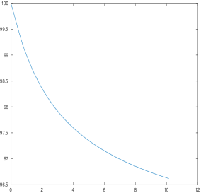
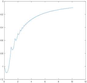
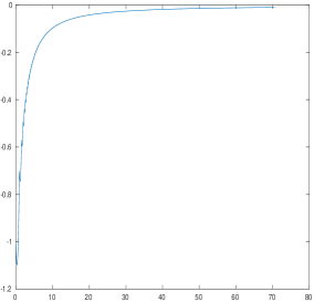
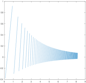
Figure 1 shows the behaviour of $f_{\mu,\eta}(x)$ for $\mu={\scriptstyle\frac{1}{2}}$ and $\eta=\varsigma={\scriptstyle\frac{1}{100}}$, its gradient and Hessian. The top three panels show the interpolated function resulting from the first 100 iterations of the ASTR1 algorithm with (3.1), while the bottom three panels report using $10^{4}$ iterations. (We have chosen to shift $f_{0}$ to 100 in order to avoid large numbers on the vertical axis of the left panels.) One verifies that the gradient is continous and converges to zero. Since the Hessian remains bounded where defined, this indicates that the gradient is Lipschitz continuous. Due to the slow convergence of the series $\sum_{j}1/j^{\frac{1}{1+2/100}}$, illustrating the boundeness of $f_{0}-f_{k+1}$ would require many more iterations. One also notes that the gradient is not monotonically increasing, which implies that $f_{\mu,\eta}(x)$ is nonconvex, although this is barely noticeable in the left panels of the figure. Note that the fact that the example is unidimensional is not restrictive, since it is always possible to make the value of its objective function and gradient independent of all dimensions but one.

Figure 1: The function $f_{\mu,\eta}(x)$ (left), its gradient $\nabla_{x}^{1}f_{\mu,\eta}(x)$ (middle) and its Hessian $\nabla_{x}^{2}f_{\mu,\eta}(x)$ (right) plotted as a function of $x$, for the first 100 (top) and $10^{4}$ (bottom) iterations of the ASTR1 algorithm with (3.1) ($\mu={\scriptstyle\frac{1}{2}}$, $\eta=\varsigma={\scriptstyle\frac{1}{100}}$)

4 A further “divergent stepsizes” variation on this theme

We now use a different proof technique to design new variants of ASTR1 with a fast global $k$-order. This is achieved by modifying the definition of the scaling factors $w_{i,k}$, requiring them to satisfy a fairly general growth condition explicitly depending on $k$, the iteration index. The motivation for introducing these new variants is their remarkable numerical performance when applied to noisy examples [17].

Theorem 4.1

Suppose that AS.1–AS.4 hold and that the ASTR1 algorithm is applied to problem (2.1), where, the scaling factors $w_{i,k}$ are chosen such that, for some power parameter $0<\nu\leq\mu<1$, all $i\in\{1,\ldots,n\}$ and some constants $\kappa_{w}\geq\varsigma_{i}\in(0,1]$, $$\varsigma_{i}\,(k+1)^{\nu}\leq w_{i,k}\leq\kappa_{w}\,(k+1)^{\mu}\;\;\;\;(k\geq 0).$$ (4.1) Then, for any $\theta\in(0,\tau\varsigma_{\min})$, $$\operatorname*{average}_{j\in\{j_{\theta}+1,\ldots,k\}}\|g_{j}\|^{2}\leq\kappa_{\diamond}\frac{(k+1)^{\mu}}{k-j_{\theta}}\leq\frac{2\kappa_{\diamond}(j_{\theta}+1)}{k^{1-\mu}},$$ (4.2) where $$j_{\theta}\stackrel{{\scriptstyle\rm def}}{{=}}\left(\frac{\kappa_{\mbox{\tiny B}}(\kappa_{\mbox{\tiny B}}+L)}{\varsigma_{\min}(\tau\varsigma_{\min}-\theta)}\right)^{{\scriptstyle\frac{1}{\nu}}}$$ (4.3) $\Gamma_{0}\stackrel{{\scriptstyle\rm def}}{{=}}f(x_{0})-f_{\rm low}$ and $$\kappa_{\diamond}\stackrel{{\scriptstyle\rm def}}{{=}}\frac{2\kappa_{w}\kappa_{\mbox{\tiny B}}}{\theta}\left(\Gamma_{0}+n(j_{\theta}+1)\frac{\displaystyle\kappa_{g}^{2}(\kappa_{\mbox{\tiny B}}+L)}{\displaystyle 2\varsigma_{\min}^{2}}\right).$$

• Proof.   From (2.11) and AS.4, using $w_{\min,j}\stackrel{{\scriptstyle\rm def}}{{=}}\min_{i\in\{1,\ldots,n\}}w_{i,k}$ ensures that

  $$\Gamma_{0}\geq f(x_{0})-f(x_{k+1})\geq\sum_{j=0}^{k}\sum_{i=1}^{n}\frac{g_{i,j}^{2}}{2\kappa_{\mbox{\tiny B}}w_{i,j}}\left[\tau\varsigma_{\min}-\frac{\kappa_{\mbox{\tiny BBL}}}{w_{\min,j}}\right].$$ (4.4)

  Consider now an arbitrary $\theta\in(0,\tau\varsigma_{\min})$ and suppose first that, for some $j$,

  $$\left[\tau\varsigma_{\min}-\frac{\kappa_{\mbox{\tiny BBL}}}{w_{\min,j}}\right]\leq\theta,$$ (4.5)

  i.e., using (4.1),

  $$\varsigma_{i}\,\,j^{\nu}\leq w_{\min,j}\leq\frac{\kappa_{\mbox{\tiny BBL}}}{\tau\varsigma_{\min}-\theta}.$$

  But this is impossible for $j>j_{\theta}$ for $j_{\theta}$ given by (4.3), and hence (4.5) fails for all $j>j_{\theta}$. But we also know from (4.1) that, for $i\in\{1,\ldots,n\}$,

  $$\left[\tau\varsigma_{\min}-\frac{\kappa_{\mbox{\tiny BBL}}}{w_{\min,j}}\right]\geq-\frac{\kappa_{\mbox{\tiny BBL}}}{\varsigma_{\min}}$$

  so that, using (4.1) and the definition of $\kappa_{\mbox{\tiny BBL}}$,

  $$\sum_{j=0}^{j_{\theta}}\sum_{i=1}^{n}\frac{\displaystyle g_{i,j}^{2}}{\displaystyle 2\kappa_{\mbox{\tiny B}}w_{i,j}}\left[\tau\varsigma_{\min}-\frac{\displaystyle\kappa_{\mbox{\tiny BBL}}}{\displaystyle w_{\min,j}}\right] \geq-\sum_{j=0}^{j_{\theta}}\frac{\displaystyle\|g_{j}\|^{2}}{\displaystyle 2\kappa_{\mbox{\tiny B}}w_{i,j}}\frac{\displaystyle\kappa_{\mbox{\tiny BBL}}}{\displaystyle\varsigma_{\min}}$$

  $$\geq-\frac{\displaystyle n\kappa_{g}^{2}(\kappa_{\mbox{\tiny B}}+L)}{\displaystyle 2\varsigma_{\min}^{2}}\displaystyle\sum_{j=0}^{j_{\theta}}\frac{\displaystyle 1}{\displaystyle(j+1)^{\nu}}$$

  $$\geq-(j_{\theta}+1)\frac{\displaystyle n\kappa_{g}^{2}(\kappa_{\mbox{\tiny B}}+L)}{\displaystyle 2\varsigma_{\min}^{2}}.$$ (4.6)

  Thus, combining (4.1), (4.4) and (4.6), we deduce that

  $$\frac{\theta}{2\kappa_{w}\kappa_{\mbox{\tiny B}}}\sum_{j=j_{\theta}+1}^{k}\frac{\|g_{j}\|^{2}}{(j+1)^{\mu}} \leq\sum_{j=j_{\theta}+1}^{k}\frac{\|g_{j}\|^{2}}{2\kappa_{\mbox{\tiny B}}w_{i,j}}\left[\tau\varsigma_{\min}-\frac{\kappa_{\mbox{\tiny BBL}}}{w_{\min,j}}\right]$$

  $$\leq\Gamma_{0}+n(j_{\theta}+1)\frac{\displaystyle\kappa_{g}^{2}(\kappa_{\mbox{\tiny B}}+L)}{\displaystyle 2\varsigma_{\min}^{2}},$$

  in turn implying that

  $$\frac{k-j_{\theta}}{(k+1)^{\mu}}\operatorname*{average}_{j\in\{j_{\theta}+1,\ldots,k\}}\|g_{j}\|^{2}\leq\frac{2\kappa_{w}\kappa_{\mbox{\tiny B}}}{\theta}\left(\Gamma_{0}+n(j_{\theta}+1)\frac{\displaystyle\kappa_{g}^{2}(\kappa_{\mbox{\tiny B}}+L)}{\displaystyle 2\varsigma_{\min}^{2}}\right),$$

  finally giving (4.2). $\Box$

We again provide some comments on this last result.

1. The choice (4.1) is of course reminiscent, in a smooth and nonconvex setting, of the “divergent stepsize” subgradient method for non-smooth convex optimization (see [2] and the many references therein), for which a ${\cal O}(1/\sqrt{k})$ global rate of convergence is known (Theorems 8.13 and 8.30 in this last reference).

2. Theorem 4.1 gives a complexity bound for iterations that are beyond an a priori computable iteration index. Indeed that $j_{\theta}$ only depends on $\nu$ and problem’s constants and, in particular does not depend on $k$. As a consequence, it can be used to determine a complexity bound to reach an iteration satisfying the accuracy requirement $\|g_{k}\|\leq\epsilon$, which is then ${\cal O}\Big{(}\epsilon^{-{\scriptstyle\frac{2}{1-\mu}}}\Big{)}+j_{\theta}(\nu)$.

3. As the chosen values of $\mu$ and $\nu$ approach zero, then the $k$-order of convergence beyond $j_{\theta}$ tends to ${\cal O}(1/\sqrt{k})$, which the order derived for the methods of the previous section and is the standard $k$-order for first-order methods using evaluations of the objective function, albeit the value of $j_{\theta}$ might increase.

4. Choosing $\nu>1$ would prevent the ASTR1 algorithm with (4.1) to converge from arbitrary starting points since then (2.2), (2.4), AS.3 and (4.1) imply that

   $$\sum_{k=0}^{\infty}\|s_{k}\|_{\infty}\leq\sum_{k=0}^{\infty}\max_{i\in\{1,\ldots,n\}}\frac{|g_{i,k}|}{w_{i,k}}\leq\kappa_{g}\sum_{k=0}^{\infty}k^{-\nu}<+\infty$$

   which would limit the distance between $x_{0}$ and any $\epsilon$-approximate first-order point.

5. Note that the requirement (4.1) allows a variety of choices for the scaling factors. Some possible choices will be explored from the numerical point of view in the next section.

We are now again interested to estimate how sharp the $k$-order bound (4.2) in ${\cal O}(\frac{1}{k^{(1-\nu)/2}})$ is.

Theorem 4.2

The bound (4.2) is essentially sharp in that, for any $\omega>{\scriptstyle\frac{1}{2}}(1-\nu)$, there exists a univariate function $f_{\omega}(x)$ satisfying AS.1–AS.4 such that the ASTR1 algorithm with (4.1) applied to this function produces a sequence of gradient norms given by $\|g_{k}\|=\frac{1}{k^{\omega}}$.

• Proof.    Consider the sequence defined, for some $\omega\in({\scriptstyle\frac{1}{2}}(1-\nu),1]$ and all $k\geq 0$, by

  $$g_{k}=-\frac{1}{k^{\omega}}\;\;\;\;w_{k}=k^{\nu},\;\;\;\;s_{k}=\frac{1}{k^{2\omega-\nu}}<1\;\;\mbox{ and }\;\;f_{k+1}=f_{k}+g_{k}s_{k},$$ (4.7)

  where we have chosen $f_{0}=\zeta(2\omega+{\scriptstyle\frac{1}{2}})$ where $\zeta(\cdot)$ is the Riemann zeta function. Immediately note that

  $$\lim_{k\rightarrow\infty}|g_{k}|=0,$$

  and $|g_{k}|\leq=1=\kappa_{g}$ for all $k$. We now verify that, if

  $$x_{0}=0\;\;\mbox{ and }\;\;x_{k}=x_{k-1}+s_{k-1}\;\;\mbox{for}\;\;k\geq 1,$$

  then exists a function $f_{\omega}(x)$ satisfying AS.1–AS.3 such that, for all $k\geq 0$,

  $$f_{\omega}(x_{k})=f_{k},\;\;\mbox{ and }\;\;g_{\omega}(x_{k})=g_{k},$$

  and such that the sequence defined by (4.7) is generated by applying the ASTR1 algorithm using $B_{k}=0$. The function $f_{\omega}(x)$ is constructed using Hermite interpolation on each interval $[x_{k},x_{k+1}]$ (note that the $x_{k}$ are monotonically increasing), which known (see [3] or [6, Th. A.9.2]) to exist whenever there exists a constant $\kappa_{f}\geq 0$ such that, for each $k$,

  $$|f_{k+1}-f_{k}-g_{k}s_{k}|\leq\kappa_{f}|s_{k}|^{2}\;\;\mbox{ and }\;\;|g_{k+1}-g_{k}|\leq\kappa_{f}|s_{k}|.$$

  The first of these conditions holds by construction of the $\{f_{k}\}_{k\geq 0}$. To verify the second, we first note that, because $1/k^{\omega}$ is a convex function of $k$ and $|1/k|\leq 1$,

  $$\frac{|g_{k+1}-g_{k}|}{|s_{k}|}\leq\frac{\omega k^{2\omega-\nu}}{k^{1+\omega}}\leq\frac{\omega}{k^{\nu-\omega+1}}\leq\omega\;\;\;\;(k\geq 0),$$ (4.8)

  where $\nu-\omega+1\geq\nu>0$, so that the desired inequality holds with $\kappa_{f}=\omega$.

  Moreover, Hermite interpolation guarantees that $f_{\omega}(x)$ is bounded below whenever $|f_{k}|$ and $|s_{k}|$ remain bounded. We have already verified the second of these conditions in (4.7). We also have from (4.7) that

  $$f_{0}-f_{k+1}=\sum_{j=0}^{k}\frac{1}{j^{2\omega}j^{\nu}}$$ (4.9)

  which converges to the finite limit $\zeta(2\omega+\nu)$ because we have chosen $\omega>{\scriptstyle\frac{1}{2}}(1-\nu)$. Thus $f_{k}\in(0,\zeta(2\omega+\nu)]$ for all $k$ and the first condition is also satisfied and AS.4 holds. This completes our proof. $\Box$

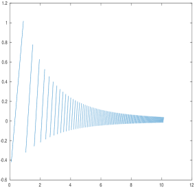
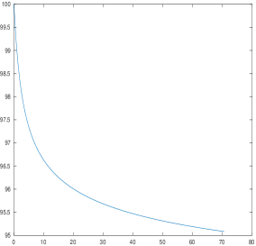
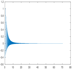
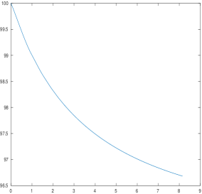
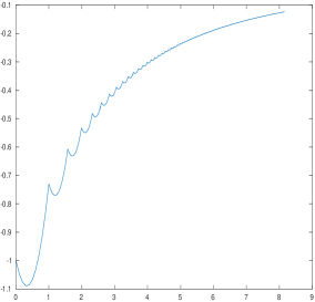
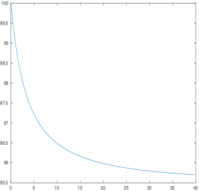
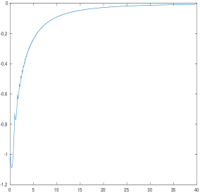
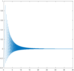
The conclusions which can be drawn from this theorem parallel those drawn after Theorem 3.4. The bound (4.2) is essentially sharp (in the sense of [5]) for the ASTR1 algorithm with (4.1). Figure 2 shows the behaviour of $f_{\omega}(x)$ for $\nu={\scriptstyle\frac{1}{9}}$ and $\omega={\scriptstyle\frac{4}{9}}+{\scriptstyle\frac{1}{100}}$, its gradient and Hessian. The top three panels show the interpolated function resulting from the first 100 iterations of the ASTR1 algorithm with (4.1), while the bottom three panels report using $5.10^{4}$ iterations. (We have again chosen to shift $f_{0}$ to 100 in order to avoid large numbers on the vertical axis of the left panels.) As above, one verifies that the gradient is continous, non-monotone and converges to zero and that the Hessian remains bounded where defined, illustrating the gradient’s Lipschitz continuity. Finally, as for Theorem 3.4, the argument in the proof of Theorem 4.2 fails for $\omega={\scriptstyle\frac{1}{2}}(1-\nu)$ because the sum in (4.9) is divergent in this case, which prevents AS.4 to hold.

Figure 2: The function $f_{\omega}(x)$ (left), its gradient $\nabla_{x}^{1}f_{\omega}(x)$ (middle) and its Hessian $\nabla_{x}^{2}f_{\omega}(x)$ (right) plotted as a function of $x$, for the first 100 (top) and $5.10^{4}$ (bottom) iterations of the ASTR1 algorithm with (4.1) ($\nu={\scriptstyle\frac{1}{9}}$, $\omega={\scriptstyle\frac{4}{9}}+{\scriptstyle\frac{1}{100}}$)

5 Numerical illustration

Because the numerical behaviour of the methods discussed above is not well-known, we now provide some numerical illustration. For the sake of clarity and conciseness, we needed to keep the list of algorithmic variants reported here reasonably limited, and have taken the following considerations into account for our choice.

1. Both scaling techniques (3.1) and (4.1) are illustrated. Moreover, since the Adam algorithm using (3.36) is so commonly used the stochastic context, we also included it in the comparison.

2. Despite Theorems 3.2 and 4.1 covering a wide choice of the parameters $\mu$ and $\nu$, we have chosen to focus here on the most common choice for (3.1) and (3.36) (i.e. $\mu={\scriptstyle\frac{1}{2}}$ and $\beta_{2}={\scriptstyle\frac{9}{10}}$, corresponding to Adagrad and Adam). When using (4.1), we have also restricted our compararison to the single choice of $\mu$ and $\nu$ used (with reasonable success) in [17], namely $\mu=\nu={\scriptstyle\frac{1}{10}}$.

3. In order to be able to test enough algorithmic variants on enough problems in reasonable computing time, we have decided to limit our experiments to low-dimensional problems. For the same reason, we have focused our experiments on the case where $\vartheta=1$.

4. We have chosen to define the step $s_{k}$ in Step 3 of the ASTR1 algorithm by approximately minimizing the quadratic model (2.10) within the $\ell_{\infty}$ trust-region using a projected truncated conjugate-gradient approach [22, 23] which is terminated as soon as

   $$\|g_{k}+B_{k}s_{k}\|_{2}\leq\max\Big{[}10^{-12},10^{-5}\|g_{k}\|_{2}\Big{]}.$$

   We also considered an alternative, namely that of minimizing the quadratic model in an Euclidean $\ell_{2}$ trust region (with the same accuracy requirement) using a Generalized Lanczos Trust Region (GLTR) technique [14].

5. We thought it would be interesting to compare “purely first-order” variants (that is variants for which $B_{k}=0$ for all $k$) with methods using some kind of Hessian approximation. Among many possibilities, we selected three types of approximations of interest. The first is the diagonal Barzilai-Borwein approximation [1]

   $$B_{k+1}=\frac{\|s_{k}\|_{2}^{2}}{y_{k}^{T}s_{k}}I_{n}$$ (5.1)

   where $I_{n}$ is the identity matrix of dimension $n$, $y_{k}=g_{k+1}-g_{k}$ and $y_{k}^{T}s_{k}>=10^{-15}\|s_{k}\|_{2}^{2}$. The second is limited-memory BFGS approximations [21], where a small number of BFGS updates are added to the matrix (5.1), each update corresponding to a secant pair $(y_{k},s_{k})$. The third is not to approximate the Hessian at all, but to use its exact value, that is $B_{k}=\nabla_{x}^{2}f(x_{k})$ for all $k$.

Given these considerations, we have selected the following algorithmic variants:

adag1 : the ASTR1 algorithm using the Euclidean $\|\cdot\|_{2}$ norm and $$w_{i,k}=\left[\varsigma+\sum_{j=0}^{k}\|g_{j}\|_{2}^{2}\right]^{\scriptstyle\frac{1}{2}}\;\;\;\;\;\;\mbox{for}\;\;i\in\{1,\ldots,n\},$$ adagi1 : the ASTR1 algorithm using the $\|\cdot\|_{\infty}$ norm and (3.1) with $\mu={\scriptstyle\frac{1}{2}}$, adag2 : the ASTR1 algorithm using the Euclidean $\|\cdot\|_{2}$ norm and $$w_{i,k}=\left[\varsigma+\sum_{j=0}^{k}\beta_{2}^{k-j}\|g_{j}\|_{2}^{2}\right]^{\scriptstyle\frac{1}{2}}\;\;\;\;\;\;\mbox{for}\;\;i\in\{1,\ldots,n\},$$ with $\beta_{2}={\scriptstyle\frac{9}{10}}$, adagi2 : the ASTR1 algorithm using the $\|\cdot\|_{\infty}$ norm and (3.36) with $\mu={\scriptstyle\frac{1}{2}}$ and $\beta_{2}={\scriptstyle\frac{9}{10}}$, maxg01 : the ASTR1 algorithm using (4.1) with $$w_{i,k}=(k+1)^{\scriptstyle\frac{1}{10}}\max\Big{[}\varsigma,\max_{j\in\{0,\ldots,k\}}\|g_{j}\|_{2}\Big{]}\;\;\;\;\;\;\mbox{for}\;\;i\in\{1,\ldots,n\},$$ maxgi01 : the ASTR1 algorithm using (4.1) with $$w_{i,k}=(k+1)^{\scriptstyle\frac{1}{10}}\max\Big{[}\varsigma,\max_{j\in\{0,\ldots,k\}}|g_{i,j}|\Big{]}\;\;\;\;\;\;\mbox{for}\;\;i\in\{1,\ldots,n\},$$ sdba : the standard steepest-descent algorithm using Armijo backtracking (see [6, Algorithm 2.2.1], for instance), b1adagi1 : adagi1 where $B_{k}$ is the Barzilai-Borwein Hessian approximation (5.1), lmadagi3b : adagi1 where $B_{k}$ is a limited-memory BFGS Hessian approximation with 3 secant pairs, Eadagi1 : adagi1 using the exact Hessian, i.e. $B_{k}=\nabla^{2}f(x_{k})$ for all $k$.

When relevant, all variants use $\varsigma=0.01$. The first seven algorithms are “purely first-order” in the sense discussed above. Note that, under AS.3, maxg01 and maxgi01 satisfy (4.1) with $\mu=\nu={\scriptstyle\frac{1}{10}}$, $\varsigma_{i}=\varsigma$ and $\kappa_{w}=\kappa_{g}$. Also note that adagi1 and adagi2 are nothing but the deterministic versions of Adagrad and Adam, respectively. All on the algorithms were run on the low dimensional instances of the problems of the OPM collection (January 2022) [19] listed with their dimension in Table 1, until either $\|\nabla_{x}^{1}f(x_{k})\|_{2}\leq 10^{-6}$, or a maximum of 100000 iterations was reached, or evaluation of the gradient returned an error.

Problem	$n$	Problem	$n$	Problem	$n$	Problem	$n$	Problem	$n$	Problem	$n$
argauss	3	chebyqad	10	dixmaanl	12	heart8ls	8	msqrtals	16	scosine	10
arglina	10	cliff	2	dixon	10	helix	3	msqrtbls	16	sisser	2
arglinb	10	clplatea	16	dqartic	10	hilbert	10	morebv	12	spmsqrt	10
arglinc	10	clplateb	16	edensch	10	himln3	2	nlminsurf	16	tcontact	49
argtrig	10	clustr	2	eg2	10	himm25	2	nondquar	10	trigger	7
arwhead	10	cosine	10	eg2s	10	himm27	2	nzf1	13	tridia	10
bard	3	crglvy	4	eigfenals	12	himm28	2	osbornea	5	tlminsurfx	16
bdarwhd	10	cube	2	eigenbls	12	himm29	2	osborneb	11	tnlminsurfx	16
beale	2	curly10	10	eigencls	12	himm30	3	penalty1	10	vardim	10
biggs5	5	dixmaana	12	engval1	10	himm32	4	penalty2	10	vibrbeam	8
biggs6	6	dixmaanb	12	engval2	3	himm33	2	penalty3	10	watson	12
brownden	4	dixmaanc	12	expfit	2	hypcir	2	powellbs	2	wmsqrtals	16
booth	2	dixmaand	12	extrosnb	10	indef	10	powellsg	12	wmsqrtbls	16
box3	3	dixmaane	12	fminsurf	16	integreq	10	powellsq	2	woods	12
brkmcc	2	dixmaanf	12	freuroth	4	jensmp	2	powr	10	yfitu	3
brownal	10	dixmaang	12	genhumps	5	kowosb	4	recipe	2	zangwill2	2
brownbs	2	dixmaanh	12	gottfr	2	lminsurg	16	rosenbr	10	zangwill3	3
broyden3d	10	dixmaani	12	gulf	4	macino	10	sensors	10
broydenbd	10	dixmaanj	12	hairy	2	mexhat	2	schmvett	3
chandheu	10	dixmaank	12	heart6ls	6	meyer3	3	scurly10	10

Table 1: The OPM test problems and their dimension

Before considering the results, we make two additional comments. The first is that very few of the test functions satisfy AS.3 on the whole of $\hbox{I\hskip-2.0ptR}^{n}$. While this is usually not a problem when testing standard first-order descent methods (because AS.3 may then be true in the level set determined by the starting point), this is no longer the case for significantly non-monotone methods like the ones tested here. As a consequence, it may (and does) happen that the gradient evaluation is attempted at a point where its value exceeds the Matlab overflow limit, causing the algorithm to fail on the problem. The second comment is that the (sometimes quite wild) non-monotonicity of the methods considered here has another practical consequence: it happens on several nonconvex problems that convergence of different algorithmic variants occurs to points with gradient norm within termination tolerance (the methods are thus achieving their objective), but these points can be quite far apart and have very different function values. It is therefore impossible to meaningfully compare the convergence performance to such points across algorithmic variants. This does reduce the set of problems where several variants can be compared.

We discuss the results of our tests from the efficiency and reliability points of view. Efficiency is measured in number of derivatives’ evaluations (or, equivalently, iterations): the fewer evaluations the more efficient the algorithm. In addition to presenting the now standard performance profile [11] for our selection of algorithms in Figure 3, we follow [25] and consider the derived “global” measure $\pi_{\tt algo}$ to be ${\scriptstyle\frac{1}{50}}$ of the area below the curve corresponding to algo in the performance profile, for abscissas in the interval $[1,50]$. The larger this area and closer $\pi_{\tt algo}$ to one, the closer the curve to the right and top borders of the plot and the better the global performance. When reporting reliability, we say that the run of an algorithmic variant on a specific test problem is successful if the gradient norm tolerance has been achieved, or if the final relative error on the objective-function value is below $10^{-7}$ or, should the optimal value be below $10^{-7}$, if the final absolute error is below $10^{-7}$. These last two criteria were applied to instances of a total of 21 problems. In what follows, $\rho_{\tt algo}$ denotes the percentage of successful runs taken on all problems were comparison is meaningful. Table 2 presents the values of these statistics in two columns: for easier reading, the variants are sorted by decreasing global performance ($\pi_{\tt algo}$) in the first, and by decreasing reliability ($\rho_{\tt algo}$) in the second.

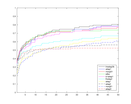
Figure 3: Performance profile for deterministic OFFO algorithms on OPM problems

algo	$\pi_{\tt algo}$	$\rho_{\tt algo}$	algo	$\pi_{\tt algo}$	$\rho_{\tt algo}$
lmadagi3b	0.72	74.79	adagi1	0.70	75.63
adagi1	0.70	75.63	b1adagi1	0.68	74.79
maxgi01	0.70	71.43	lmadagi3b	0.72	74.79
sdba	0.69	73.95	sdba	0.69	73.95
b1adagi1	0.68	74.79	maxgi01	0.70	71.43
Eadagi1	0.60	67.23	adag1	0.54	68.91
adag1	0.54	68.91	Eadagi1	0.60	67.23
adag2	0.52	36.13	maxg01	0.52	63.03
maxg01	0.52	63.03	adag2	0.52	36.13
adagi2	0.51	31.09	adagi2	0.51	31.09

Table 2: Performance statistics for deterministic OFFO algorithms on OPM problems

A total of 22 problems could not be successfully solved by any of the above algorithms, we believe mostly because of ill-conditioning.

The authors are of course aware that the very limited experiments presented here do not replace extended numerical practice and could be completed in various ways. They nevertheless suggest the following (very tentative) comments.

1. There seems to be a definite advantage in using the $\|\cdot\|_{\infty}$ norm over $\|\cdot\|_{2}$, as can be seen by comparing adag1 with adagi1, adag2 with adagi2, and maxg01 with maxgi01. While this may be due in part to the fact that the trust region in $\ell_{\infty}$ norm is larger than that in $\ell_{2}$ norm (and thus allows larger steps), it is also the case that the disaggregate definition of the scaling factors $w_{i,k}$ ((3.1), (3.36) or (4.1)) used in conjunction with the $\ell_{\infty}$ norm may allow a better exploitation of differences of scale between coordinates.

2. Among the ”purely first-order” methods, sdba, maxgi01 and adagi1 are almost undistinguishable form the performance point of view, with a small reliability advantage for adagi1 (Adagrad). This means that, at least in those experiments, the suggestion resulting from the theory that OFFO methods may perform comparably to standard first-order methods seems vindicated.

3. The Adam variants (adag2 and adagi2) are clearly outperformed in our tests by the Adagrad ones (adag1 and adagi1). We recall that analytical examples where Adam fails do exist, while the convergence of Adagrad is covered by our theory.

4. The theoretical difference in global rate of convergence between adagi1 and maxgi01 does not seem to have much impact on the relative performance of these two methods.

5. The use of limited memory Hessian approximation (lmadagi1) appears to enhance the performance of adagi1, but this is not the base of the Barzilai-Borwein approximation (b1adagi1) or, remarkably, for the use of the exact Hessian (Eadagi1). When these methods fail, this is often because the steplength is too small to allow the truncated conjugate-gradient solver to pick up second-order information in other directions than the negative gradient. What favours the limited memory approach remains unclear at this stage.

Finally, and although this is a slight digression from the paper’s main topic, we report in Table 3 how reliability of our selection of OFFO variants is impacted by noise. To obtain these results, we ran the considered methods on all test problems where the evaluations (function and derivatives) are contaminated by 5, 15, 25 or 50 % of relative Gaussian noise with unit variance. The reliability percentages in the table result from averaging ten sets of independent runs.

	$\rho_{\tt algo}$/relative noise level
algo	0%	5%	15%	25%	50%
adagi1	75.63	70.42	70.34	72.02	72.77
b1adagi1	74.79	75.38	75.13	75.38	75.88
lmadagi3b	74.79	74.79	70.67	71.34	71.09
sdba	73.95	34.29	35.04	36.30	36.89
maxgi01	71.43	70.59	70.42	73.61	74.45
adag1	68.91	64.12	68.91	71.09	71.01
Eadagi1	67.23	67.98	68.74	70.17	70.08
maxg01	63.03	63.28	59.50	61.60	63.70
adag2	36.13	28.74	30.76	39.16	42.35
adagi2	31.09	24.12	25.88	28.66	31.93

Table 3: Reliability of OFFO algorithms as a function of the relative Gaussian noise level

As can be seen in the table, the reliability of the sdba methods dramatically drops as soon as noise is present, while that of the other OFFO methods is barely affected and remains globally unchanged for increasing noise levels. This is consistent with widespread experience in the deep learning context, where noise is caused by sampling among the very large number of terms defining the objective function. This observation vindicates the popularity of methods such as Adagrad in the noisy context and suggests that the new OFFO algorithms may have some practical potential.

6 Conclusions

We have presented a parametric class of deterministic “trust-region minded” extensions of the Adagrad method, allowing the use of second-order information, should it be available. We then prove that, for OFFO algorithms in this class, $\min_{j\in\{0,\ldots,k\}}\|g_{j}\|={\cal O}(1/\sqrt{k+1})$. This bound, which we have shown to be essentially sharp, is identical to the global rate of convergence of standard first-order methods using both objective-function and gradient evaluations, despite the fact that the latter exploit significantly more information. Thus, if one considers the order of global convergence only, evaluating the objective-function values is an unnecessary effort. We have also considered another class of OFFO algorithms inspired by the “divergent stepsize” paradigm in non-smooth convex optimization and have provided an essentially sharp (but slighlty worse) global rate of convergence for this latter class. Limited numerical experiments suggest that the above theoretical conclusions may translate to practice and remain, for OFFO methods, relatively independent of noise.

Although discussed here in the context of unconstrained optimization, adaptation of the above OFFO algorithms to problems involving convex constraints (such as bounds on the variables) is relatively straightforward and practical: one then needs to intersect the trust-region with the feasible set and minimize the quadratic model in this intersection (see [8, Chapter 12]). It will be also of interest to further analyze the possible links between our proposals and those of [16], both from the theoretical and practical perspectives.