The White Dwarf Binary Pathways Survey VI: two close post common envelope binaries with TESS light curves

Abstract

Establishing a large sample of post common envelope binaries (PCEBs) that consist of a white dwarf plus an intermediate mass companion star of spectral type AFGK, offers the potential to provide new constraints on theoretical models of white dwarf binary formation and evolution. Here we present a detailed analysis of two new systems, TYC 110-755-1 and TYC 3858-1215-1. Based on radial velocity measurements we find the orbital periods of the two systems to be $\sim 0.85$ and $\sim 1.64$ days, respectively. In addition, HST spectroscopy of TYC 110-755-1 allowed us to measure the mass of the white dwarf in this system ($0.78\,\mathrm{M}_{\odot}$). We furthermore analysed TESS high time resolution photometry and find both secondary stars to be magnetically extremely active. Differences in the photometric and spectroscopic periods of TYC 110-755-1 indicate that the secondary in this system is differentially rotating. Finally, studying the past and future evolution of both systems, we conclude that the common envelope efficiency is likely similar in close white dwarf plus AFGK binaries and PCEBs with M-dwarf companions and find a wide range of possible evolutionary histories for both systems. While TYC 3858-1215-1 will run into dynamically unstable mass transfer that will cause the two stars to merge and evolve into a single white dwarf, TYC 110-755-1 is a progenitor of a cataclysmic variable system with an evolved donor star.

1 Introduction

Close white dwarf (WD) binaries are the result of the evolution of main sequence star binaries. After the more massive star evolves into a giant star it may fill its Roche lobe and the resulting mass transfer is typically dynamically unstable. As a consequence the entire binary evolves through a common envelope (CE) (e.g., Taam & Ricker, 2010; Passy et al., 2011; Ivanova et al., 2013). During this phase, angular momentum and orbital energy are extracted from the orbit and unbind the envelope (Webbink, 1984; Zorotovic et al., 2010), revealing a close binary containing a white dwarf and its main-sequence companion. These systems, known as post-common-envelope binaries (PCEBs), are thought to be the progenitors of some of the most exotic objects in the Galaxy, such as cataclysmic variables (Warner, 1995a), AM CVn binaries (Warner, 1995b), hot subdwarf stars (Heber, 2009), supersoft X-ray sources (SSSs, Kahabka & van den Heuvel, 1997), and double degenerates binaries (Webbink, 1984). The latter two are progenitor candidates for type Ia supernovae (SNe Ia, Bildsten et al., 2007; Wang & Han, 2012). The zoo of possible evolutionary outcomes demonstrate the complexity of close white dwarf binary evolution.

Important progress towards our understanding of close compact binary star evolution has been derived from surveys of PCEBs (Rebassa-Mansergas et al., 2007; Rebassa-Mansergas et al., 2012; Nebot Gómez-Morán et al., 2011). These surveys provided constraints on the common envelope efficiency (Zorotovic et al., 2010) and the subsequent angular momentum loss due to magnetic braking (Schreiber et al., 2010). However, these works were entirely focused on PCEBs composed of a white dwarf and a low-mass (M < 0.4 M_⊙) main-sequence (spectral type M) companion. If angular momentum loss drives the systems close enough to initiate the mass transfer from the main-sequence star to the white dwarf, this mass transfer will be stable given the small mass ratio, i.e. virtually all PCEBs with M dwarf companion will become CVs sooner or later which then may evolve towards shorter orbital periods or merge due to consequential angular momentum loss (Schreiber et al., 2016). In other words, previous surveys of PCEBs do not provide constraints on the formation mechanism of objects as important as SSSs and double degenerates which must form from PCEBs with secondary stars more massive than M dwarfs.

The main aim of the white dwarf binary pathways survey project is to extend the search for PCEBs towards systems containing secondary stars of A, F, G or K spectral type (WD+AFGK). A sufficiently large sample of this type of systems will provide new constraints on the close white dwarf binary formation. Additionally, they provide potentially large implications for our understanding of close white dwarf binary formation and evolution, including the two main channels that are thought to produce a type Ia supernovae.

We established a large target sample ($\sim 1600$) of WD+AFGK binary stars combining ultraviolet (UV) observations from GALEX with optical wavelengths observations from the Radial Velocity Experiment (RAVE, Kordopatis et al., 2013) in Parsons et al. (2016, hereafter paper I), the Large Sky Area Multi-Object Fibre Spectroscopic Telescope (LAMOST, Deng et al., 2012) in Rebassa-Mansergas et al. (2017a, hereafter paper II) and more recently with the Tycho-Gaia Astrometric Solution (TGAS, Lindegren et al., 2016) described in Ren et al. (2020, hereafter paper V). So far, this search has resulted in the discovery of TYC 6760-497-1, the first known pre-SSS binary (Parsons et al., 2015), followed by TYC 7218-934-1, a triple system whose discovery led us to estimate the fraction of triple systems that could contaminate the WD+AFGK sample to be less than 15 per cent (Lagos et al., 2020, hereafter paper III). Finally, we recently showed that rather similar close white dwarf binaries with G-type star companions can have quite distinctive futures (Hernandez et al., 2021, hereafter paper IV).

Among the systems we identified is one object that will likely evolve into a SSS. As SSSs are difficult to observe due to their short lifetime and because the X-ray emission is hard to detect as it is easily absorbed by neutral hydrogen in the galactic plane, observing progenitors of SSSs might represent our best chance to provide observational constraints on this evolutionary channel. We also found a system that will evolve into a CV with an evolved donor. These systems are thought to be one of the possible progenitors of AM CVn stars with an estimated birthrate through this channel of ($0.5-1.3$)$\times 10^{-3}yr^{-1}$ in our Galaxy (Podsiadlowski et al., 2003). The third system we found will lead to a dynamical merger of the WD and the secondary star when the latter is on the asymptotic giant branch (AGB). The combination of the extreme mass ratio and the convective envelope of the giant star causes unstable mass transfer onto the WD driving to the formation of a common envelope. The merger of the WD with the massive degenerate core of the AGB star may lead to a SN Ia explosion through the so–called core degenerate scenario which could produce $\sim 1-2$ per cent of these events (Zhou et al., 2015).

Here we present two additional close binaries discovered by our project, TYC 110-755-1 and TYC 3858-1215-1 (hereafter TYC 110 and TYC 3858, respectively), composed of a white dwarf with a G and K type secondary star, respectively, and with orbital periods shorter than two days.

2 Observations

White dwarfs with AFGK spectral type are much more difficult to identify in observational surveys than WD+M binaries as the main sequence companion star dominates the emission at optical wavelength. The target selection of The White Dwarf Binary Pathways Survey is therefore based on combining information from optical surveys with GALEX data (for details see ; , ). In this paper we present two of the selected targets that turned out to be close white dwarf binaries: TYC 110 and TYC 3858. We characterize both systems combining photometric and spectroscopic observations and in what follows we describe in detail the performed observations and data reduction.

2.1 Optical high resolution spectroscopy

After identifying TYC 110 and TYC 3858 as PCEB candidates from TGAS and LAMOST samples ( ; , respectively), we performed time-resolved high-resolution optical spectroscopic follow up observations to confirm their close binarity by means of radial velocity variations. Thanks to our targets being bright ($V=10.5$ mag and $11.48$ mag, for TYC 110 and TYC 3858 respectively) the observations were performed under poor weather conditions.

Observations with three different high-resolution spectrographs installed at different telescopes were obtained for both systems. We used the Echelle SPectrograph from REosc for the Sierra San pedro martir Observatory (ESPRESSO, Levine & Chakarabarty, 1995) at the 2.12 m telescope of the Observatorio Astronómico Nacional at San Pedro Mártir (OAN-SPM), México and observed with the Ultraviolet and Visual Echelle Spectrograph (UVES, Dekker et al., 2000) on the Very Large Telescope of the European Southern Observatory (ESO) in Cerro Paranal. Additional data were obtained with the High Resolution Spectrograph (HRS, Jiang, 2002) at the Xinglong 2.16 m telescope (XL216) located in China.

ESPRESSO provides spectra covering the wavelength range from $3500$ to $7105$ Å  with a spectral resolving power of R $\approx 18\,000$ for a slit width of 150 $\mu$m. A Th-Ar lamp before each exposure was used for wavelength calibration. HRS provides spectra of a $49\,800$ resolving power for a fixed slit width of 0.19 mm and covers a wavelength range of $\sim 3650$–$10\,000$ Å. Th-Ar arc spectra were taken at the beginning and end of each night. The ESPRESSO and HRS spectra were reduced using the echelle package in IRAF. Standard procedures, including bias subtraction, cosmic-ray removal, and wavelength calibration, were carried out using the corresponding tasks in IRAF. The observations carried out with UVES have a spectral resolution of 58 000 for a 0.7–arcsec slit. With its two-arms, UVES covers the wavelength range of $3000$–$5000$ Å  (blue) and $4200$–$11\,000$ Å  (red), centered at 3900 and 5640 Å  respectively. Standard reduction was performed making use of the specialized pipeline EsoReflex workflow (Freudling et al., 2013).

2.2 HST spectroscopy

The presence of a white dwarf in our WD+AFGK binary star candidates is inferred from UV excess emission in GALEX. We have previously observed ten candidate systems with the Hubble Space Telescope (paper I) and in all cases the presence of a white dwarf was confirmed which indicates that our selection algorithm is very efficient and that our target sample is rather clean. However, excess UV emission or optical spectroscopy does not provide solid constraints on the mass of the white dwarf. The only way to reliably measure the white dwarf mass is through ultraviolet spectroscopy.

We obtained far-ultraviolet (FUV) spectroscopy of TYC 110 using the Space Telescope Imaging Spectrograph (STIS, Kimble et al., 1998) on-board the HST (GO 16224) on 2021 January 31. Spectra were obtained over one spacecraft orbit, resulting in a spectrum with total exposure time of 2185 seconds. They were acquired with the MAMA detector and the G140L grating. The spectra cover a wavelength range of 1150–1730 Å  with a resolving power between 960–1440. The FUV spectra were reduced and wavelength calibrated following the standard STIS pipeline (Sohn et al., 2019). The HST spectrum contains emission lines of He II at 1640 Å  and C IV at 1550 Å, and shows the broad Ly-alpha absorption of a hydrogen white dwarf atmosphere.

2.3 TESS photometry

Motivated by the idea to measure the main sequence star rotational periods, and resolve if the secondary stars in close binary stars are indeed tidally locked,we extracted high cadence light curves for both systems from the TESS database (Ricker et al., 2015). The TESS mission splits observations into 26 overlapping 24x96 degree sky sectors over the Northern and Southern hemispheres; and each sector was observed for approximately one month. The light curves were downloaded from the Mikulski Archive for Space Telescopes (MAST) web service. TYC 110 data belong to sectors 5 and 32, while TYC 3858 was observed in sectors 15, 16, 22 and 23. The time covered by each sector can be found in Table 1. Pre-search Data Conditioned Simple Aperture Photometry (PDCSAP) flux was used for this study.

3 Stellar and orbital parameters

The performed observations allow us to characterize the stellar and orbital parameters of both systems. We describe in this section the characterization of the secondary star and the determination of the orbital period from our high resolution spectroscopic observations and TESS photometry. The white dwarf parameters for TYC 110 are then determined from our HST observations.

3.1 The secondary stars

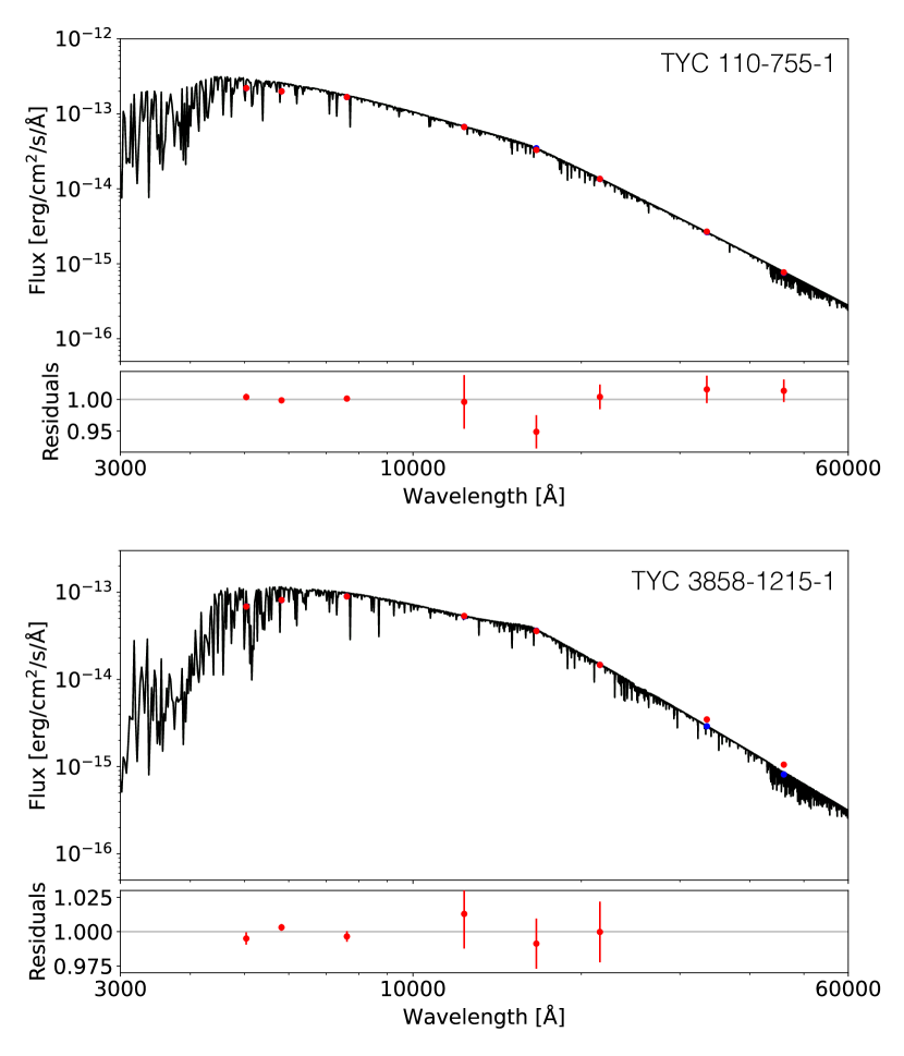
Figure 1: Spectral energy distributions created from $G_{\mathrm{BP}}$, $G_{\mathrm{RP}}$ and $G$ Gaia bands, $J$, $H$ and $K_{s}$ band data from 2MASS, and $W1$ and $W2$ band data from WISE (red dots) were fitted with MARCS.GES theoretical spectra (black line).

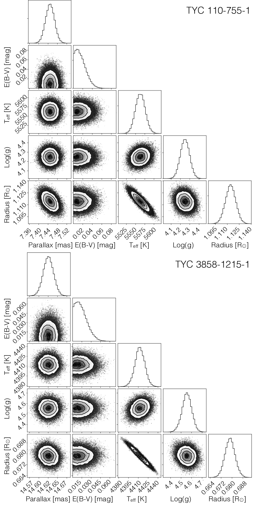
Figure 2: Posterior probability distributions for model parameters obtained from the SED fit.

To determine the stellar parameters of the main-sequence star in our binaries, normalized spectra with the highest signal-to-noise ratio of each target were fitted to MARCS.GES models (Gustafsson et al., 2008) using iSpec (Blanco-Cuaresma et al., 2014), allowing to measure the effective temperatures ($T\mathrm{{}_{eff}}$), surface gravities ($\log{g}$), metallicities ($Z$) and rotational broadening ($v\sin{i}$) for our targets. The spectral fitting procedure started with different initial values. On the one hand we used the Gaia DR2 (Gaia Collaboration et al., 2018) $T\mathrm{{}_{eff}}$ values, $\log{g}$=4.5 dex, $v\sin{i}$=10 km s^-1 and solar metallicity. On the other hand, fits were also performed with initial values varied by $\pm$100 K in $T\mathrm{{}_{eff}}$, using $\log{g}$=4.0 dex and 5.0, metallicities of $Z=-1$ and +0.5 dex, and $v\sin{i}$=1 and 100 km s^-1 in order to ensure that all fits converge to the same solution.

The resulting best-fit model was combined with the spectral energy distribution (SED) of the target scaled to Gaia EDR3 (Gaia Collaboration, 2020) parallaxes (7.44(01) mas for TYC 110 and 14.62(01) mas for TYC 3858) to estimate the radius of the secondary star. The SED of our targets were created using the Gaia EDR3 $G_{\mathrm{BP}}$, $G_{\mathrm{RP}}$ and $G$ bands, along with $J$, $H$ and $K_{s}$ band data from 2MASS (Cutri et al., 2003), and $W1$ and $W2$ band data from WISE (Cutri & et al., 2012). It is worth highlighting that the photometry for TYC 3858 is affected by several nearby stars, rendering the $W1$ and $W2$ band data unreliable for this object because of the spatial resolution, so they were not included in the fit. The Gaia and 2MASS data appear to be unaffected by this. The SED fit uses the parallax, reddening, $T\mathrm{{}_{eff}}$, $\log{g}$ and radius as initial parameters for the Markov chain Monte Carlo (MCMC) method (Press et al., 2007) to determine the final values and their uncertainties. $T\mathrm{{}_{eff}}$ and $\log{g}$ are initialised based on the values from the spectral fit, while in the case of the parallax and reddening we use the priors and parameter ranges constrained by Gaia EDR3 (Lallement et al., 2019) and the STILISM reddening map (Capitanio et al., 2017) which provide uncertainties. In any case, given the distance and location of our targets we expect reddening to be negligible. The radius is initialised at a sensible value for a main sequence star with the corresponding $\log{g}$ and $T\mathrm{{}_{eff}}$. The production chain used 50 walkers, each with 10 000 points. The first 1500 points were classified as a "burn-in", and were removed from the final results. The best fit values and their uncertainties are listed in Table 2. For both stars, the obtained stellar parameters do not correlate with the small reddening, and the obtained reddening is even consistent with zero, which makes sense given the high latitude and the close distance to these targets and which is in agreement with the value provided by the Gaia/2MASS 3D extinction map . The obtained SEDs and parameter distributions of both targets are plotted in Fig. 1 and 2, respectively.

3.2 Radial velocities

Radial velocities (RVs) from ESPRESSO and UVES spectra were computed using the cross-correlation technique against a binary mask representative of a G-type star. The uncertainties in radial velocity were computed using scaling relations (Jordán et al., 2014) with the signal-to-noise ratio and the width of the cross-correlation peak, which was calibrated with Monte Carlo simulations.

Radial velocities from the spectra collected with the HRS spectrograph were obtained by fitting the normalised Ca II absorption triplet (at $8498.02,8542.09$, and $8662.14$ Å) with a combination of a second order polynomial and a triple-Gaussian profile of fixed separations, as described in Rebassa-Mansergas et al. (2017b). The radial velocity uncertainty is obtained by summing the fitted error and a systematic error of 0.5 km s^-1 in quadrature (paper V). All radial velocities and observing details obtained for TYC 110 and TYC 3858 are provided in table 5 and 6 of the appendix.

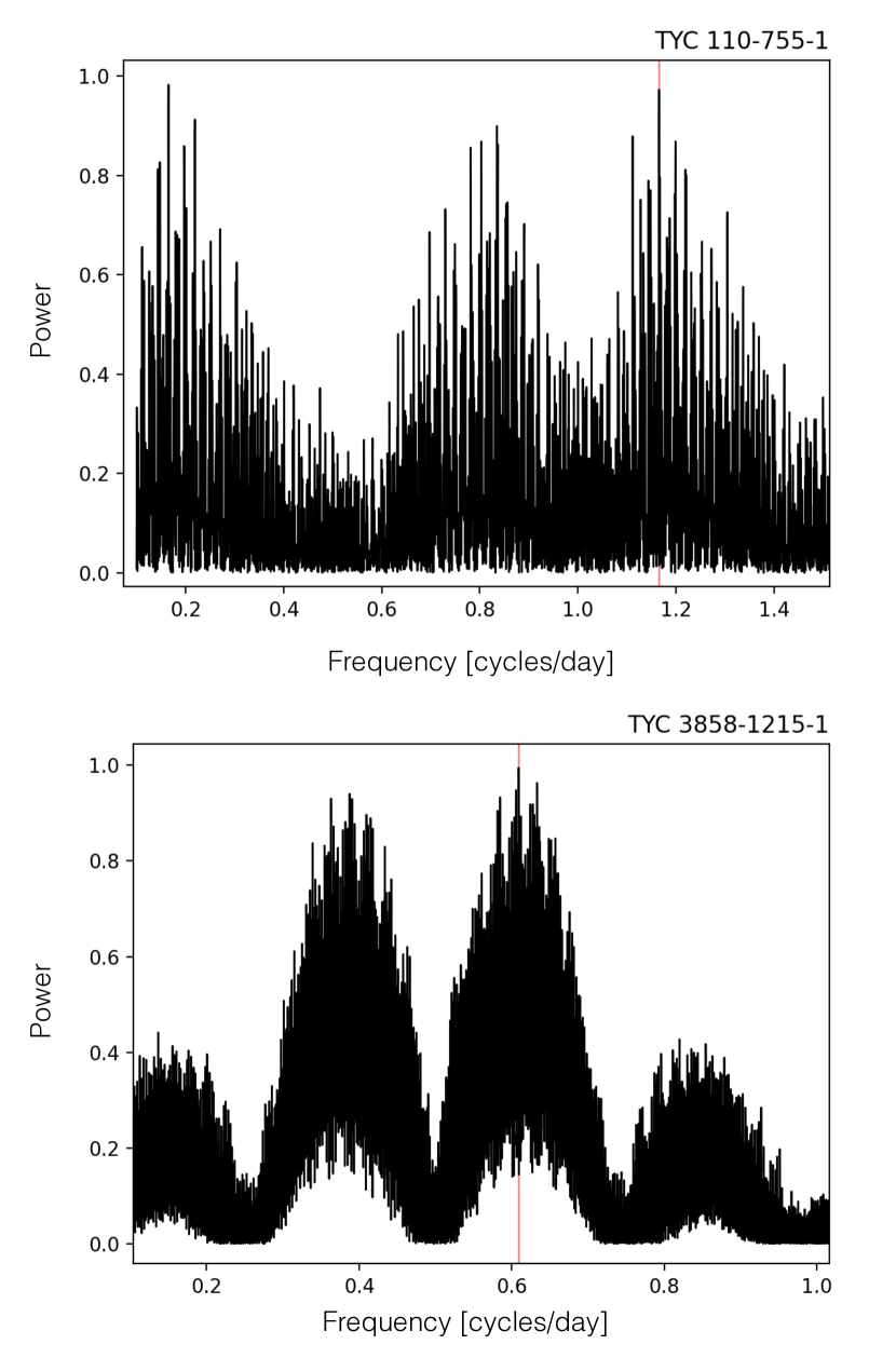
Figure 3: Lomb-Scargle periodograms based on the spectroscopic observations of TYC 110 (top) and TYC 3858 (bottom). The red lines highlight the highest peak which corresponds to the orbital period of the systems.

We used the least-squares spectral analysis method based on the Generalized Lomb-Scargle Periodogram (GLS Zechmeister et al., 2009), implemented in the astroML python library (VanderPlas et al., 2012), to identify the orbital period of both systems. Additionally, a specialized Monte Carlo sampler created to find converged posterior samplings for Keplerian orbital parameters called The Joker (Price-Whelan et al., 2017; Price-Whelan et al., 2020) was used. The Joker is especially useful for non-uniform data and also allows to identify eccentric orbits. As we have previously identified a system with an eccentric orbit which turned out to be a triple star system with a white dwarf component (paper III), double-checking circular orbits derived from Lomb-Scargle periodograms was absolutely required, especially for TYC 3858 which is a hierarchical triple system where the PCEB is the inner binary. The third object is an M-dwarf star at $\sim 330$ au from the inner binary, far away enough to not have any significant impact on the ultraviolet detection or to affect on some way the evolution of the PCEB. We discovered the third object by searching the Gaia EDR3 for sources around the system with consistent parallaxes and proper motions.

The GLS periodograms of the RV measurements for both systems are shown in Fig. 3. Folding the radial velocity data with the best period yields the radial velocity curves shown in Fig. 4. Data from different telescopes are plotted in different colors. The measured orbital periods for TYC 110 and TYC 3858 are 0.858 and 1.6422 days, respectively. The eccentricity in both cases is negligible.

While the best fit period provides a reasonable representation of the data, the periodograms show several aliases with similar powers to the selected period. We tested with the three highest peaks for each target and find that the selected period reproduces the data best but that the second highest peaks provide only a factor of 8 and 1.5 larger $\chi^{2}$ values for TYC 110 and TYC 3858, respectively. Our radial velocity data alone does therefore not provide an unambiguous orbital period measurement. However, as we shall see in the next section, TESS photometry available for both targets clearly breaks the degeneracy and confirms that the best fit periods are the correct orbital periods in both cases.

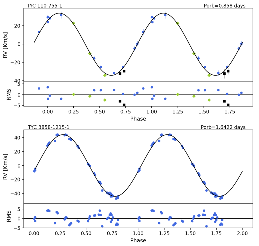
Figure 4: Phase-folded radial velocity curves for the main-sequence stars in TYC 110 (top) and TYC 3858 (bottom), with the corresponding residuals to the best fit. The colors indicate which instrument was used to obtain the measurement: OAN-SPM (blue circles), XL216 (black squares), and UVES (green diamonds).

3.3 Photometric observations

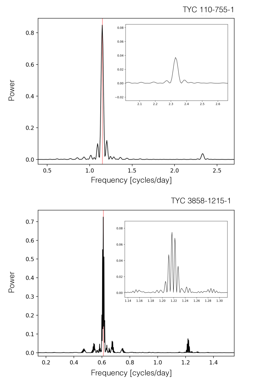
Figure 5: The power spectra of TYC 110 (top) and TYC 3858 (bottom) calculated for their TESS light curves combining data from all sectors. The inserted zoom corresponds to the small range of frequencies around the second peak found at half the orbital period.

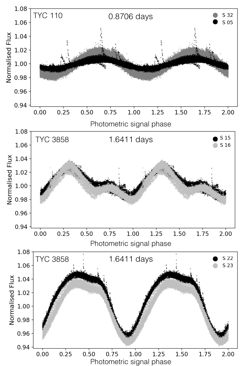
Figure 6: The upper panel shows the TESS light curve of TYC 110 in sector 5 (black points) and 32 (grey points). The rotational period is consistent between the two sectors, but there is a change in the amplitude of the variations. We split the light curve of TYC 3858 into two different plots to better visualise the changes in shape and amplitude over time. In the middle panel, observations show sector 15 (black) and 16 (grey) with an amplitude of $\sim$1.7 percent. In the bottom panel, which shows data from sector 22 (black) and 23 (grey), the amplitude increases to $\sim$4.2 percent.

We applied the least-squares spectral analysis method based on the classical Lomb-Scargle periodogram (Lomb, 1976; Scargle, 1982) to the TESS data of both systems (see Fig. 5). We also removed the dominant photometric period from both data sets and investigated the residuals. The phase folded light curve for both targets are shown in Fig. 6. We found the light curve of TYC 110 is rather sinusoidal with short term variations that we interpret as flares. TYC 3858 shows a double-peaked feature and also some flare activity. Shape and amplitude of the light curve change from one epoch to the other for both targets while the periodicity of the signal for the individual sectors are identical within the uncertainties. Table 1 shows the periods and amplitudes measured from each sector for both systems. In what follows we discuss the results obtained from the TESS light curves in the light of the spectroscopic period for both binary stars.

Table 1: List of the periods and amplitudes obtained by analyzing individual sectors of TESS observations of each system. The last column shows the flux that was used to normalize the corresponding light curve.

Target/	Time range	Period	Amplitude	Flux zero
sector	[BJD]	[days]	[$e^{-}$/s]	[$e^{-}$/s]
TYC 110-755-1
05	2458437.99–2458463.94	0.870$\pm$0.005	120.4$\pm$0.4	18309
32	2459174.23–2459199.97	0.871$\pm$0.004	279.8$\pm$0.2	18640
TYC 3858-1215-1
15	2458711.36–2458735.69	1.65$\pm$0.07	160.7$\pm$0.6	9637
16	2458738.64–2458762.64	1.60$\pm$0.07	172.0$\pm$0.9	9606
22	2458899.89–2458926.49	1.64$\pm$0.02	206.5$\pm$0.8	9713
23	2458930.21–2458954.87	1.64$\pm$0.03	398.9$\pm$0.8	9584

3.3.1 TYC 110-755-1

The main period we found for TYC 110 is $0.87066\pm 0.00099$ days which is close to the best fit spectroscopic period with a difference of 18 minutes. On one hand this suggest that the period we selected from the radial velocities corresponds to the orbital period. On the other hand, the difference between the radial velocity period and the period obtained from the TESS light curve is larger than the combined period uncertainties. This result is very puzzling at first glance as the general hypothesis is that for binaries with orbital periods shorter than 10 days synchronised rotation can be assumed for main sequence stars (Fleming et al., 2019).

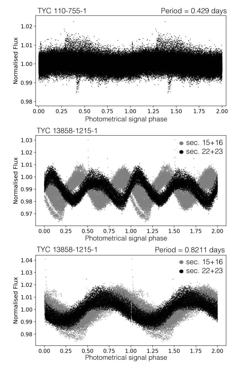
Figure 7: Variation detected in the TESS light curves after removing the main photometric signal. Top: Ellipsoidal variation found in TYC 110 (sector 32). The data is phase folded over a period 0.429 days which corresponds to exactly half the orbital period obtained from our radial velocity measurements. Middle: Variation detected in TYC 3858, sectors 15 $+$ 16 (gray) and 22 $+$ 23 (black) after removing the main signal and phase folded over the periods 0.82055 and 0.82202 days, respectively. Bottom: Variation found in TYC 3858 after a second round of subtracting a sinusoidal fit. The residuals are phase folded over a period 0.8211 days which corresponds to exactly half the orbital period obtained from our radial velocity measurements. The signals at half the orbital period are not caused by ellipsoidal variations in the case of TYC 3858 because their amplitude largely exceeds the expected amplitude for ellipsoidal variations given the system parameters. Instead we suggest that spots at roughly opposite sides of the secondary star might cause the observed periodicities.

However, by further investigating the TESS light curve we found a possible solution for this problem. After removing the main periodic signal from the TESS light curve, we found a statistically significant signal with a period of $0.4290$ days, i.e. exactly half the spectroscopic period (Fig. 5). This signal is consistent with being caused by ellipsoidal variations given that according to the measured stellar masses and radius of the secondary, the latter is filling approximately 66 per cent of its Roche-lobe. The resulting light curve is shown in Fig. 7. The measured amplitude of the signal is $0.106\pm 0.002$ percent of the measured flux. To further test our hypothesis that this signal corresponds to ellipsoidal variations, we calculate the theoretically predicted amplitude of ellipsoidal variations using the measured stellar and binary parameters of the system. According to Morris & Naftilan (1993) and Zucker et al. (2007) the relative flux produced by ellipsoidal variations is given by

$$\frac{\delta F}{F}=0.15\frac{(15+u_{1})(1+\beta_{1})}{(3-u_{1})}\left(\frac{R_{1}}{a}\right)^{3}q\sin^{2}{i},$$ (1)

where $\frac{\delta F}{F}$ is the fractional semi-amplitude of the ellipsoidal variation, star 1 refers to the main-sequence star, $u_{1}$ is the linear limb darkening coefficient and $\beta_{1}$ is the gravity darkening exponent for the main-sequence star in the TESS filter, which we obtained from tables 24 and 29 of Claret (2017). $R_{1}$ is the radius of the main-sequence star, $a$ is the semi-major axis, $q=M_{WD}/M_{1}$ is the mass ratio and $i$ is the system inclination. We found that using the parameter from Table 2 the theoretical predicted values for the amplitude of ellipsoidal variations for TYC 110 cover the range of $0.137-0.172$ percent of the measured flux, which is in good agreement with the value measured from the light curve. This result confirms that the spectroscopic period is the orbital period of the binary star system and the signal at half the orbital period is most likely caused by ellipsoidal variations.

To understand the difference in the rotational and orbital period of the secondary star, a closer look at the period variations over time is required. In Fig. 8 we show the residuals as a function of orbital cycle number and find that there clearly is a variation in the light curve that changes over time. We interpret this as being caused by differential rotation of the secondary star, i.e. while the equatorial regions are synchronised with the orbital motion, at higher latitudes this might not be the case, or vice versa. If a starspot is moving to a different latitude, which rotates at a slightly slower velocity, the spot comes into view out-of-time on each orbit, resulting in a longer period. The position of the starspots moving on the surface of the star may also cause the amplitude variation we observed in the light curve shown in Fig. 6.This scenario is plausible as it is common for solar type stars to be differentially rotating. This has been seen in some donor stars in cataclysmic variables and other non-eclipsing binaries (Lurie et al., 2017; Bruning, 2006; Maceroni et al., 1990). Finally, TYC 110 clearly shows flares in its light curves which further supports our moving starspot interpretation of the observed periodicities.

3.3.2 TYC 3858-1215-1

TYC 3858 has been covered in 4 TESS sectors, hence, a large amount of data is available for this target. In contrast to TYC 110, the TESS period of TYC 3858 is entirely consistent with the spectroscopic period in all four sectors. However, as illustrated in Fig. 5, apart from the orbital period, we also find a strong signal (with several peaks close to each other) at half the orbital period. In what follows we investigate the origin of these signals.

We first divided the TESS light curve in two parts according to their shapes and times when the data was taken, one for sectors $15+16$ and one for $22+23$. We then fitted a sinusoid with the spectroscopic period to each pair of sectors and removed it from the light curve. We clearly see sinusoidal variations in the residuals but with a different period, i.e. $0.82055(12)$ and $0.82202(88)\,$days for sector $15\,+\,16$ and $22\,+\,23$, respectively, and with a significant phase shift between the two parts of the light curve. The residuals are plotted together (middle panel in Fig. 7) phase folded over their period.

Given that several peaks are seen in the power spectrum close to half the orbital period, we proceeded by subtracting the sinusoidal signal observed in the residuals and again investigated the residuals. The result (Fig. 7 bottom panel) shows a light curve with a period exactly half the orbital period (0.821100(75) days) with reasonable phase alignment. The relative amplitudes for both sectors agrees within the errors.

In what follows we interpret the above described findings in the light of the system parameters derived previously. First, the signal at nearly half the orbital period obtained after subtracting the main signal (which corresponds to the orbital period) cannot be caused by ellipsoidal variations. The observed change in period between sector $15+16$ and $22+23$ might appear relatively small but it is statistically significant and, more importantly, the strong phase shift between both light curves cannot be explained by the uncertainty of the measured orbital period. This phase shift excludes ellipsoidal variations as the origin of the observed signal. This conclusion is further strengthened by the amplitude of the signal, $0.90\pm 0.01$ and $0.87\pm 0.03$ percent for sectors $15+16$ and $22+23$, respectively, which is far larger than the amplitude predicted by Eq. 1. Even if we let the white dwarf mass vary between $0.2$ and $1.4\mathrm{M}_{\odot}$, the predicted amplitude ranges from $0.018$ to $0.092$ percent which is more than an order of magnitude below the measured amplitude. It is impossible to match the measured amplitude without significantly increasing the radius of the main-sequence star (by a factor of 2.1), which would be incompatible with the SED fit and Gaia parallax.

Given that the signal in the residuals after subtracting the two main periods is found at half the orbital period, both amplitude and period do not significantly vary between the different sectors, and there is no significant phase shift, one might think that this signal now is finally caused by ellipsoidal variations. However, the amplitude of the observed signal ($0.90\pm 0.003$ percent for sectors $15+16$ and $0.85\pm 0.004$ percent for the sectors $22+23$) remains an order of magnitude larger than predicted for ellipsoidal variations. Again, this difference cannot be explained by the uncertainties in the stellar or binary parameters.

We propose a different explanation which, as in the case of TYC 110, is related to the activity of the secondary star. Assuming that two large star spots (or several smaller ones) are located at roughly opposite sides of the secondary star, one would expect brightness variations close to half the orbital period and, as these star spots might slightly move and/or appear/reappear at different latitudes on the K-star surface, one would also expect the obtained periods to somewhat vary with time. This scenario could also explain why we see a large number of periods close to half the orbital period in the power spectrum (Fig. 5). In addition, the idea is not in conflict with the measured amplitudes. We therefore conclude that, while it is difficult to provide definitive prove, a reasonable interpretation of the signals at half the orbital is that they are related to the spatial distribution of star spots on the surface of the active secondary star.

This overall interpretation is consistent with the trailed plot (Fig. 8) which shows that there are plenty of residual patterns, but these do not move in phase as in the case of TYC 110. The variations can be associated with new spots appearing at a different place on the surface of the K-type secondary star, rather than the same spots moving. While there is no clear evidence of differential rotation in the light curve of TYC 3858, the system clearly shows flare activity in agreement with our interpretation of the variations in the light curve shape and the periodic signals found close to half the orbital period.

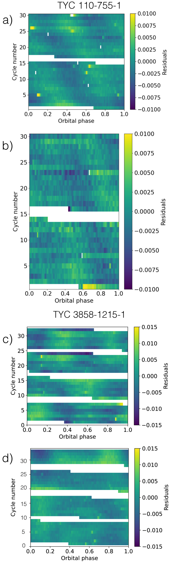
Figure 8: Evolution of the light curve of TYC 110 (upper panel, a and b belongs to sector 5 and 32, respectively) and TYC 3858 (bottom panel, c and d belongs to sector 15+16 and 22+23, respectively) to illustrate the spots migration. The average light curve has been subtracted; the plot shows the residual light curve for each cycle corresponding to the light curve folded on the orbital period.

3.4 The white dwarfs

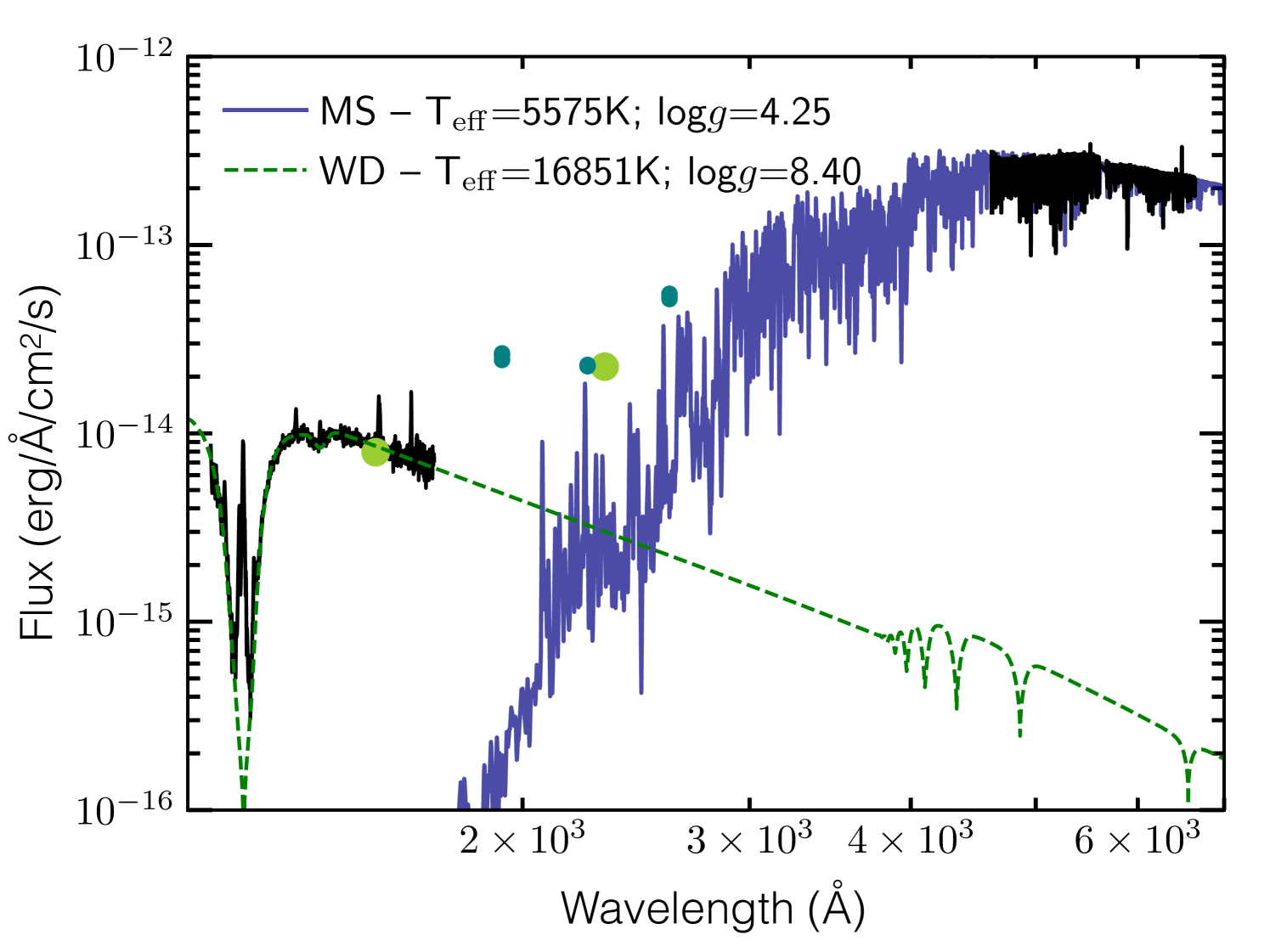
Figure 9: The SED of TYC 110-755-1 from ultraviolet to optical wavelength ranges. The black lines are the observed UV HST/STIS spectrum and optical UVES spectrum (no telluric correction was applied). The best-fitting BT-NextGen main-sequence star model is shown in dark blue and was rotationally broadened to match the measured value for the main-sequence star in TYC 110. The light-green dots represent $FUV$ and $NUV$ GALEX observations and in small teal dots UVOT observations from Swift. We also plot with a green dashed line a pure-hydrogen synthetic model for a $T_{\mathrm{eff}}$=16 851 K and $\log{g}$=8.40 dex white dwarf. We note that the combined flux of our white dwarf model and the model for the secondary star fail to reproduce the NUV measured with GALEX and Swift. We assume that model of the G-type secondary star is underpredicting the NUV emission as chromospheric emission is not taken into account but likely occurring in active G-type stars.

We applied the MCMC technique to fit the HST/STIS spectrum of TYC 110 using the emcee python package (Foreman-Mackey et al., 2013). We started by generating a grid that spans from 9000–30 000 K (with steps of 200 K) and 7.00–8.50 (in steps of 0.1) for the effective temperature and the surface gravity of pure hydrogen atmosphere white dwarfs (Koester, 2010). The mixing length parameter for convection was set to 0.8. Then we fitted the HST spectrum under two assumptions (1) by including a BT-NextGen model for the secondary star and (2) by ignoring possible contributions from the secondary. We found that the results do not differ which confirms that the secondary does not contribute to the far UV emission. Henceforth we consider just a white dwarf model to fit the HST spectrum.

For the reddening we also used two approaches. First, we assumed the same prior as in the case of the secondary star (restricting the reddening according to the range of values provided by Stilism and second we assumed the fixed value taken from the Gaia/2MASS map, i.e. E($B-V$)=0.0048 mag (Lallement et al., 2019). The latter value is at the low end of the range of values obtained from fitting the secondary star (which basically does not constrain the reddening, see Fig.2). The values derived for the white dwarf parameters using the different approaches concerning the reddening differ by less than eight percent which does not affect any of our conclusions. In Table 2 we list the values obtained from assuming the lower value of the reddening which we consider more realistic given the distance and location of the target.

We set a flat prior on the parallax using the EDR3 Gaia parallax of 7.44 mas. In contrast, the surface gravity and effective temperature are constrained to be within the limits of the synthetic grid. We set 100 walkers to sample the parameter space with 5000 steps to assure convergence of the chains. The likelihood function to maximize was defined as $-0.5\chi^{2}$. The best fit parameters are found by using the median of the marginalized distributions of the parameters and their errors: $\Pi=7.454(1)$ mas, $T_{\mathrm{eff}}=16\,851(35)$ K, $\log{g}=8.396(8)$ dex. The best fit model spectrum is shown in Fig. 9 together with the spectrum and model of the secondary star.

The mass and the radius of the white dwarf are a function of the surface gravity and effective temperature through the mass-radius relation for white dwarfs. We used the mass-radius relation for white dwarfs with hydrogen-rich atmospheres by interpolating the cooling models from Fontaine et al. (2001) with thick hydrogen layers of M${}_{\rm H}/$M${{}_{\mathrm{WD}}}=10^{-4}$. We used the last 100 steps of the effective temperature and surface gravity chains to sample the mass-radius relation which does not depend significantly on the assumed thickness of the atmosphere. This produces two distributions (one for the mass and another for the radius). The best values of mass and radius for the white dwarf were extracted with the marginalized distributions and we obtained: M${}_{\mathrm{WD}}=$ 0.784(3) M_⊙ and R${}_{\mathrm{WD}}=$ 0.0107(4) R_⊙.

In the case of TYC 3858 the presence of a white dwarf has not yet been unambiguously confirmed. However, assuming the UV excess coming from a white dwarf companion appears reasonable given that so far all 11 WD+AFGK candidate systems that have been observed with HST indeed contained a white dwarf. Knowing the secondary mass and the orbital period, it is possible to estimate the minimum white dwarf mass (0.147 and 0.214 M_⊙ for TYC 110 and TYC 3858, respectively) if we assume an orbital inclination of 90 degrees. Additionally, it is known that in binaries with short orbital periods the secondary is tidally locked (Fleming et al., 2019). A range of possible white dwarf masses (0.497–0.597 $M_{\odot}$ for TYC 110 and 0.214–0.676 $M_{\odot}$ for TYC 3858) can therefore be estimated using the binary mass function based on $v\sin{i}$ and radius measurements of the secondary star. However, one has to keep in mind that we derive the secondary star parameters by fitting single main sequence star model spectra to observed spectra of Roche-distorted secondary stars in close binaries, and therefore the white dwarf masses derived from the radius and $v\sin{i}$ have to be considered as rather rough estimates.

Indeed, comparing the white dwarf masses derived from the HST spectrum of TYC 110 with our estimate based on $v\sin(i)$, we find a strong disagreement which clearly illustrates that the latter estimate is very uncertain. All estimated masses, derived from HST spectral fitting, the minimum white dwarf mass, and the estimate based on $v\sin{i}$ and synchronised rotation, are shown in Table. 2.

Table 2: Stellar and binary parameters obtained for the two PCEBs presented in this work. The values provided for the reddening represent the result obtained from the fitting of the secondary star (assuming a prior corresponding to the range of values obtained from Lallement et al. (2019)). For the fitting of the HST spectrum of the white dwarf in TYC 110 we assumed the value provided by the Gaia/2MASS extinction map which is consistent with the range of values obtained from the fit of the secondary star but at the lower end (which we consider the most realistic assumption).

Parameter	TYC 110-755-1	TYC 3858-1215-1
Orbital Period [days]	0.85805 $\pm 0.00001$	1.6422 $\pm 0.0008$
Phase zero [BJD]	2458544.287 $\pm$ 0.003	2458404.262 $\pm$ 0.003
E[$B-V$]	0.014 $\pm 0.13$	0.013$\pm 0.012$
Distance [pc]	134.24 $\pm 0.34$	68.43 $\pm 0.88$
Inclination [deg]	18.67 - 21.49	25.33 - 86.64
Sec. Amplitude [km s-1]	34.21 $\pm 0.80$	44.28 $\pm$ 0.40
Sec. $v\sin{i}$ [km s-1]	22.42 $\pm 1.51$	27.0 $\pm 18.0$
$V_{\gamma}$ [km s-1]	-7.6 $\pm 0.6$	-17.4 $\pm 0.3$
Sec. Luminosity [L⊙]	1.065 $\pm 0.006$	0.156 $\pm 0.001$
Sec. log g [dex]	4.24 $\pm 0.05$	4.55 $\pm 0.04$
Sec. Z [dex]	-0.14$\pm 0.14$	0.15$\pm 0.37$
Sec. $T_{\mathrm{eff}}$ [K]	5562.83 $\pm 13.15$	4412.31 $\pm 7.53$
Sec. Radii [R⊙]	1.114 $\pm 0.006$	0.679 $\pm 0.004$
Sec. Mass [M⊙]	0.80 $\pm 0.09$	0.61 $\pm 0.07$
Sec. type	G4V	K3VI
WD minimum Mass [M⊙]	-	0.214
WD Mass(i) [M⊙]	-	0.214 - 0.676
$\ast$WD Mass [M⊙]	0.784 $\pm 0.03$	-
$\ast$WD $T_{\mathrm{eff}}$ [K]	16 851 $\pm 35$	-
$\ast$WD log g [dex]	8.39 $\pm 0.00$	-
$\ast$WD Radii [R⊙]	0.0107 $\pm 0.0004$	-

We obtained the phase zero, amplitude and $v\sin{i}$ from the radial velocities measurements.
$V_{\gamma}$ is the radial velocity of the center of mass of the system.
The white dwarf Mass(i) corresponds to $v\sin{i}$ method.
$\ast$ HST spectra fitting.

4 Scrutinizing the unusual emission lines in TYC 110-755-1

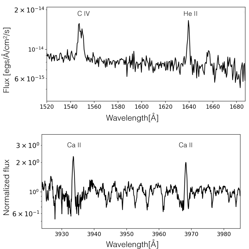
Figure 10: Two small portions of the full spectra of TYC 110-755-1. The strong He II line at 1640 Å  and C IV at 1550 Å  observed in the HST spectra are shown in the upper panel, while the chromospherical emission lines of Ca II at 3933.66 and 3968.47 Å  in the optical range are shown in the bottom panel.

As we have learned in the previous sections, TYC 110 shows multiple signs of chromospheric/magnetic activity typical for G-stars such as spots, flares, and now chromospheric emission lines such as H_α, and Ca II (Fig. 10). However, in addition to these rather typical features strong He II line at 1640 Å  and C IV at 1550 Å  (see Fig. 10) are found in the HST-UV spectrum. While the most natural explanation is that these emission lines are related to activity as well, for completeness we tested the alternative possibility that wind accretion onto a magnetic white dwarf is the origin of the UV-emission lines as accretion onto the magnetic poles could produce such emission lines.

To that end, we observed TYC 110 using Swift orbital telescope as a target of opportunity (ToO target ID:14068) from February 22 to March 7, 2021. One orbit exposures were obtained per day to cover at least two orbital periods, with a total on-source exposure time of 23 165 sec. The average count rate is 0.043 counts per second. Sixteen Swift orbits covered all orbital phases of the object evenly. We used the X-ray Telescope (XRT, Burrows et al., 2005) and the Ultraviolet/Optical Telescope (UVOT, Roming et al., 2005) to analyse data for the presence of possible pulses produced by a spinning magnetic white dwarf. Standard data processing was made later at the Swift Science Data Centre. The data were collected with the XRT operating in AUTO mode. Simultaneous UV images in the $UVW1$, $UVW2$ and $UVM2$ at 2600, 1928 and 2246 Å, respectively, were obtained with the UVOT. We used an on-line tool to extract the XRT light curve and standard aperture photometry using Web-HERA provided by The High Energy Astrophysics Science Archive Research Center (HEASARC, Blackburn et al., 1999), corresponding procedures to measure UV fluxes. In both cases HEASOFT v6.28 software and calibration were used.

No significant phase-dependent variability was detected, neither at X-ray nor at UV wavelengths. Hence, we omit unnecessary figures to present these data. However, UV measurements (two for each $UVW1$, $UVW2$ and $UVM2$ bands) are presented in Fig. 9 (small dark green dots). We note that the flux in the NUV predicted by the models obtained from our spectral fitting is not sufficient to reproduce the observations. We assume that this is most likely a consequence of chromospheric emission of the secondary star in the NUV which is not considered in the models.

Despite being difficult to prove, this hypothesis appears reasonable as large differences between predicted and observed NUV fluxes for active stars have been reported previously. For example, the chromospheres of active M dwarfs can fully dominate their NUV fluxes, i.e. the photospheric flux predicted by model spectra is underestimating the NUV flux of these stars by orders of magnitude (Stelzer et al., 2013, their figures 6 and 7). In addition, for evolved stars a relation between excess NUV flux and rotation has been found (Dixon et al., 2020) and for fast rotators the NUV flux from the chromosphere exceeds that of the photosphere by up to four magnitudes (see also Jayasinghe et al., 2021, their figure 19).

While these results are not directly applicable to the G type secondary star in TYC 110, given the fast rotation of the star and the fact that is showing strong signs of activity in its light curve, it is plausible that steady chromospheric emission which is not incorporated in the model spectra is responsible for the large discrepancy between our fits and the observations in Fig. 9.

As the Swift observations did not confirm the magnetic white dwarf hypothesis, we conclude that the system is a PCEB with a particularly active secondary star and that the emission lines are a result of this activity. In fact, in certain aspects the system resembles V471 Tau (Sion et al., 2012) which also contains a rapidly rotating main sequence K-star with spots and flare activity. V471 Tau also shows emission lines in the UV, including C IV and He II, and is an X-ray source.

5 Past and future evolution

Previous attempts to understand the formation and evolution of close white dwarf binaries, particularly with massive companions (AFGK), indicate that, to unbind the common envelope from the binary, the energy needed might be higher than in those systems with M-dwarf companions (e.g., Zorotovic et al., 2014b, a). However, in recent papers we presented four systems with G-type secondaries that do not support that hypothesis (paper I, paper IV).

With the aim of further constraining theories of close compact binary star evolution, we have reconstructed the past evolution of the two systems following paper IV, i.e. using the algorithm developed by Zorotovic et al. (2010), leaving the common envelope efficiency ($\alpha_{\mathrm{CE}}$) as a free parameter and assuming that no other sources of energies (like the hydrogen recombination energy) contributed to the ejection process. Table 3 lists the reconstructed parameters of the possible progenitors for both systems. The first row for each system corresponds to the reconstructed parameters assuming the same efficiency derived for PCEBs consisting of a white dwarf and an M-dwarf companion from SDSS (i.e., $\alpha_{\mathrm{CE}}=0.2-0.3$, Zorotovic et al. 2010), while the second row is for the whole range of possible efficiencies. For TYC 110 we provide the results for the more reliable mass of the white dwarf based on HST spectral fitting. As for the three systems studied in paper IV, TYC 110 and TYC 3858 do not require extra energy sources, apart from the available orbital energy, to have survived a common-envelope phase, regardless of the set of derived parameters assumed for the reconstruction of TYC 110. Given their short current orbital periods, TYC 3858 can be reconstructed with virtually any value of $\alpha_{\mathrm{CE}}\leq 1$ while for TYC 110 and the HST spectral fitting imply $\alpha_{\mathrm{CE}}\geq 0.19$. For TYC 110 we found possible progenitors for the whole range of derived white dwarf masses. The parameters derived from the HST spectral fitting imply a massive progenitor that filled its Roche lobe during the thermally pulsing asymptotic giant branch phase when the system was very young. For TYC 3858, on the other hand, the common envelope reconstruction imposes a lower limit of $0.27\,M_{\odot}$ on the white dwarf mass, and the progenitor of the white dwarf may have filled its Roche lobe either on the first giant branch or on the asymptotic giant branch.

Table 3: Reconstructed binary parameters assuming common envelope evolution. $M_{\mathrm{1,i}}$ and $P_{\mathrm{orb,i}}$ are the initial primary mass and initial orbital period, respectively. For each system, the first row lists the parameters constraining $\alpha_{\mathrm{CE}}$ in the range of 0.2-0.3, while the second row is for any $\alpha_{\mathrm{CE}}\leq 1$.

Object	$\alpha_{\mathrm{CE}}$	WD Mass [M⊙]	$M_{\mathrm{1,i}}$ [M⊙]	$P_{\mathrm{orb,i}}$ [days]	CE Age[Gyr]
TYC 110 ( HST )	0.2–0.3	0.75–0.82	3.24–3.71	929–1947	0.26–0.38
	0.19–1.0	0.75–0.82	3.15–3.75	147–2015	0.26–0.42
TYC 3858	0.2–0.3	0.34–0.62	0.98–2.11	103–1477	1.29–13.29
	0.03–1.0	0.27–0.68	0.98–2.98	22–1591	0.49–13.29

WD+AFGK binaries are crucial for our understanding of close white dwarf binary formation not only because these systems constrain common envelope evolution theories but also because we can estimate the future evolution of these systems using detailed simulations. While white dwarfs with late-type secondary stars will all become cataclysmic variables when the secondary fills its Roche lobe, the future of PCEBs with solar type secondary stars depends on several factors such as the orbital period at the end of common envelope evolution, the angular momentum loss mechanism that drives the system to shorter orbital periods, the mass ratio of the binary, and the evolutionary status of the secondary star.

The three systems shown in paper IV provide evidence for the diversity of evolutionary futures of close WD+AFGK binaries and we here further confirm this finding. TYC 110 contains a G-type secondary star like in the cases of TYC 4700-815-1, TYC 1380-957-1 and TYC 4962-1205-1, while TYC 3858 contains a K-type secondary star, and all these binaries have orbital periods between 0.85 and 2.5 days. Despite their similarities, the future of these systems are quite different. With the aim to predict how these systems will evolve and what kind of interacting binary stars they will form in the future, we performed dedicated simulations using MESA (Paxton et al., 2011), with the same set-up and the same criteria for stable mass transfer as in Parsons et al. (2015) and paper IV. For each system we adopt the parameters listed in Table 2.

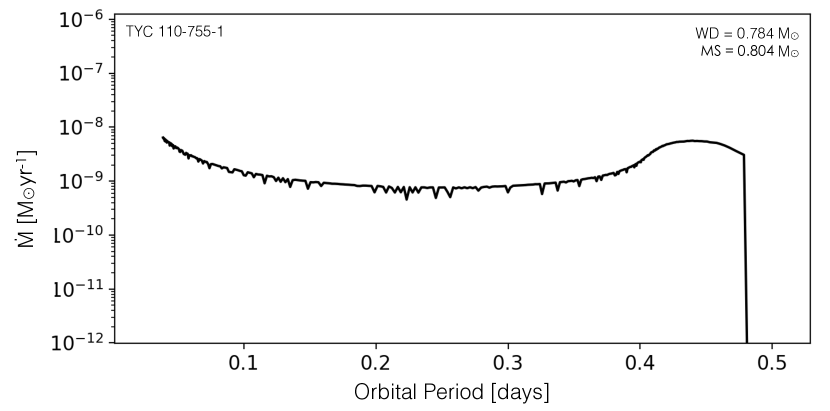
Figure 11: The future evolution of TYC 110-755-1 for a white dwarf with the HST mass estimation of 0.78 M_⊙ and a main sequence star of 0.804 M_⊙. This system will become a cataclysmic variable with an evolved donor star. Mass transfer mainly driven by magnetic breaking will continue during the orbital period range of 2-3 hr.

Simulations for TYC 110 were performed assuming a secondary mass of M${}_{\mathrm{MS}}=0.804$ M_⊙, a white dwarf mass of M${}_{\mathrm{WD}}=0.78$ M_⊙, the current orbital period of the system $\mathrm{P_{orb}}=0.858$ days and the current radius of the secondary star of R${}_{\mathrm{MS}}=1.114$ R_⊙. The radius of TYC 110 is larger than that of a star of the same mass on the zero age main sequence (ZAMS), which indicates that the secondary is slightly evolved. The starting model for our MESA simulations was obtained by evolving the secondary until it reaches the required radius of the evolved secondary star. Due to the large white dwarf mass, mass transfer remains dynamically and thermally stable and the system evolves into a CV. In 15 Myr from now, when the orbital period has been reduced to 11 hrs, mass transfer starts but never reaches values large enough to ignite stable nuclear burning on the surface of the white dwarf. In this case nova eruptions should occur and the mass of the white dwarf remains nearly constant (non-conservative mass transfer). Thus, TYC 110 will evolve into a CV with a significantly evolved secondary. Driven out of thermal equilibrium due to mass transfer, the evolved secondary does not become fully convective and angular momentum loss through magnetic braking will be efficient leading to large mass transfer rates until it reaches the orbital period minimum of $\sim\,0.932$ hrs in 57 Myr. The system will not evolve as a detached system through the orbital period gap (see Fig. 11). This evolutionary path for cataclysmic variables with evolved secondary stars has been predicted by Kolb & Baraffe (2000) and several such CVs have been found (e.g. Thorstensen et al., 2002; Rebassa-Mansergas et al., 2014).

The future of TYC 3858 is straightforward to predict. Given the mass ratio of 0.79 < $q$ < 3.17 where $q=M_{MS}/M_{WD}$, the secondary mass of $0.61\,M_{\odot}$ and radius of $0.68\,R_{\odot}$ the system will run into dynamically unstable mass transfer when the secondary fills its Roche-lobe in 2 Gyr from now, when the orbital period will be 6 hrs. This is predicted by our MESA simulations in agreement with Ge et al. (2015). The orbital energy of the binary will not be sufficient to expel the envelope and therefore the two stars will merge and evolve into a giant star with the core of this giant being the white dwarf we observe today. This giant will then evolve into a single white dwarf as the final fate of TYC 3858.

In Table 4 we list the orbital periods of all PCEBs with secondary stars earlier than M. Thanks to our survey a population of systems with short orbital periods (below 1-2 days) could be established. At the same time, a population of systems with significantly longer orbital periods (weeks to years) exists. If these indications for a bimodal distribution can be confirmed due to further observations, the population of WD+AFGK binaries might consist of two sub-samples that perhaps formed through different evolutionary channels.

Table 4: list of known WD+AFGK PCEBs sorted by orbital period. We include the two systems described in this work.

Object	Porb [days]	Msec [M⊙]	MWD [M⊙]	Reference
GPX-TF16E-48	0.2975	0.64	0.72	7
TYC 6760-497-1	0.4986	1.23	0.52–0.67	5
V471 Tau	0.5208	0.93	0.84	6
TYC 110-755-1	0.858	0.84	0.784	9
TYC 4962-1205-1	1.2798	0.97	0.59–0.77	8
TYC 1380-957-1	1.6127	1.18	0.64–0.85	8
TYC 3858-1215-1	1.6422	0.61	0.22-0.68	9
TYC 4700-815-1	2.4667	1.45	0.38–0.44	8
IK Peg	21.722	1.70	1.19	1
KOI-3278	88.1805	1.05	0.634	2
SLB3	418.72	1.56	0.62	3
KIC 8145411	455.87	1.12	0.197	4
SLB1	683.27	1.106	0.53	3
SLB2	727.98	1.096	0.62	3

1-Wonnacott et al. (1993), 2-Kruse & Agol (2015), 3-Kawahara et al. (2018), 4-Masuda et al. (2019), 5-Parsons et al. (2015), 6-O’Brien et al. (2001), 7-Krushinsky et al. (2020), 8-paper IV, 9-This work.

6 Conclusions

We presented the discovery of two post common envelope binaries (PCEBs) with intermediate mass (G and K spectral type) secondary stars. We used high resolution optical spectroscopy to determine stellar parameters of the secondary star of both systems, and STIS HST spectroscopy to determine the white dwarf parameters of TYC 110.

Based on the orbital and stellar parameters obtained from these observations, we reconstruct the past and predict the future evolution of both systems. We find that both systems join the class of close WD+AFGK stars that do not require any modifications of the common envelope prescription when compared to PCEBs with M-dwarf companions. Our systematic survey of WD+AFGK binary stars has now discovered six such systems (this paper, paper IV and Parsons et al. (2015)) which clearly indicates that a population of PCEBs with secondary stars earlier than M exists that forms through common envelope evolution in the same way as PCEBs with M-dwarf companions. Given that reconstructing the evolution of two other close WD+AFGK systems, IK Peg and KOI-3278 (Zorotovic et al., 2014b), does require additional energy sources during common envelope evolution, one might speculate that two different populations of WD+AFGK binaries emerge from the first mass transfer phase which, if confirmed, might have far reaching consequences for our understanding of close white dwarf binary formation.

If this finding can be further confirmed, an immediate question that arises is whether the longer orbital period systems are absent among close WD+M binaries. As there is no obvious reason why the common envelope efficiency should be higher for some WD+AFGK binaries and why additional sources of energy should be available for some of them, we speculate that the longer orbital period systems among WD+AFGK stars are perhaps the result of dynamically stable mass transfer. This type of mass transfer requires mass ratios close to one for the main sequence progenitor systems. As these mass ratios are impossible for the progenitors of WD+M binaries, this scenario naturally explains why longer orbital period systems are not found among them. While two populations of post mass transfer WD+AFGK binaries, one with short orbital periods from CE evolution and one with longer orbital periods emerging from stable mass transfer is therefore a tempting interpretation of the results obtained so far, more observations are needed to establish the existence of two different populations.

While the main focus of our survey is to progress with our understanding of white dwarf binary formation and evolution, in this work we learned that PCEBs with earlier secondary stars are excellent laboratories for studying magnetic activity. Using detailed TESS light curves of both systems studied here, we find that both systems have rapidly rotating secondary stars and show plenty of flares and starspots. Nevertheless, the difference between both systems can not be more sharp. While TYC 3858 shows short-lived spots that appear to remain mostly fixed, TYC 110 shows long-lived spots that migrate across a differentially rotating surface. We also found that TESS light curves can be used to identify close binaries in our targets sample, which will reduce the amount of required spectroscopic follow-up observations.

The future of the two systems we presented in this work will be very different. TYC 3858 will run into dynamically unstable mass transfer and evolve into a single white dwarf while TYC 110 will evolve into a cataclysmic variable star with an evolved donor star. Combining this finding with the results obtained by Parsons et al. (2015) and paper IV who found systems that evolve into the same channels or into thermal time scale mass transfer (becoming super soft sources for some time) we conclude that small changes in the system parameters can drastically change the fate of these systems. This is because, for these earlier spectral type secondary stars, the critical mass ratios for stable as well as dynamically and thermally unstable mass transfer are relatively close to each other. This emphasizes the importance of conducting a WD+AFGK binary survey, since a large sample of observationally well characterized systems can provide crucial constraints for white dwarf binary evolution theory with implications for the SN Ia progenitor problem.

Data Availability

The data underlying this article will be shared on reasonable request to the corresponding author.

Appendix A Radial velocities

Table 5: TYC 110-755-1 Radial velocity measurements.

Instrument	S/N	Exptime	BJD	RV	error
		$s$		$Km~{}s^{-1}$	$Km~{}s^{-1}$
ESPRESSO	30	1200	2458450.8084	5.53	1.33
ESPRESSO	28	1200	2458451.7378	21.91	0.72
ESPRESSO	33	1200	2458804.7751	-23.08	1.13
ESPRESSO	34	1200	2458176.0456	-39.90	2.10
ESPRESSO	29	1200	2458857.7013	24.18	1.51
ESPRESSO	31	1200	2458859.7440	-32.70	0.76
ESPRESSO	33	1200	2458860.7120	-39.23	1.17
ESPRESSO	30	1200	2458861.7381	-12.33	0.91
ESPRESSO	28	1200	2458915.6990	-32.55	1.09
ESPRESSO	29	1200	2458916.6745	-7.18	1.03
ESPRESSO	33	1200	2458917.6707	20.54	0.55
HRS	45	2400	2458170.0718	-37.20	1.40
HRS	35	1000	2458172.032480	-5.70	4.50
UVES	69	120	2458355.850589	15.06	0.61
UVES	64	120	2458356.842519	-17.95	0.64
UVES	69	120	2458357.824764	-41.62	0.64

Table 6: TYC 3858-1215-1 Radial velocity measurements.

Instruments	S/N	Exptime	HJD	RV	error
		$s$		$Km~{}s^{-1}$	$Km~{}s^{-1}$
ESPRESSO	26	1200	2457945.7164	-61.78	0.86
ESPRESSO	29	1200	2457946.7218	10.56	0.81
ESPRESSO	25	1200	2457947.6950	-22.02	0.80
ESPRESSO	20	1200	2457951.6644	8.09	0.75
ESPRESSO	30	1200	2457948.6984	-40.83	0.86
ESPRESSO	31	1200	2457953.6797	-53.32	0.90
ESPRESSO	28	1200	2458277.7669	-25.55	0.86
ESPRESSO	25	1200	2458277.7811	-24.00	0.82
ESPRESSO	29	1200	2458278.7998	-40.90	0.74
ESPRESSO	31	1200	2458278.8141	-43.20	0.64
ESPRESSO	30	1200	2458279.7631	26.40	0.80
ESPRESSO	27	1200	2458856.9729	-56.22	0.89
ESPRESSO	24	1200	2458856.9870	-56.93	0.87
ESPRESSO	28	1200	2458857.0012	-57.96	0.87
ESPRESSO	24	1200	2458857.0174	-57.61	1.18
ESPRESSO	29	1200	2458857.0316	-57.54	1.12
ESPRESSO	31	1200	2458857.0457	-59.06	1.13
ESPRESSO	32	1200	2458857.9501	26.17	0.77
ESPRESSO	30	1200	2458857.9642	26.90	0.64
ESPRESSO	29	1200	2458857.9784	26.37	0.59
ESPRESSO	26	1200	2458858.0227	20.73	0.69
ESPRESSO	28	1200	2458858.0368	20.32	0.70
ESPRESSO	34	1200	2458858.0510	19.56	0.75
ESPRESSO	36	1200	2458859.9596	-14.97	0.95
ESPRESSO	31	1200	2458859.9737	-16.42	0.93
ESPRESSO	33	1200	2458859.9879	-18.09	0.99
ESPRESSO	29	1200	2458860.0571	-28.72	0.75
ESPRESSO	28	1200	2458860.0713	-31.23	0.83
ESPRESSO	29	1200	2458860.9626	10.95	0.87
ESPRESSO	31	1200	2458860.9770	13.40	0.93
ESPRESSO	30	1200	2458860.9911	15.23	0.92
ESPRESSO	33	1200	2458861.0794	17.98	0.80
ESPRESSO	27	1200	2458861.9640	-61.94	0.71
ESPRESSO	29	1200	2458861.9790	-61.64	0.75
ESPRESSO	28	1200	2458861.9932	-60.82	0.73
ESPRESSO	30	1200	2458862.0432	-64.90	0.87
ESPRESSO	31	1200	2458862.0574	-64.09	0.90
ESPRESSO	26	1200	2458862.0717	-64.16	0.91
ESPRESSO	28	1200	2458279.7775	26.79	0.84

References

- Bildsten et al. (2007) Bildsten L., Shen K. J., Weinberg N. N., Nelemans G., 2007, ApJ, 662, L95
- Blackburn et al. (1999) Blackburn J. K., Shaw R. A., Payne H. E., Hayes J. J. E., Heasarc 1999, FTOOLS: A general package of software to manipulate FITS files (ascl:9912.002)
- Blanco-Cuaresma et al. (2014) Blanco-Cuaresma S., Soubiran C., Heiter U., Jofré P., 2014, A&A, 569, A111
- Bruning (2006) Bruning D. H., 2006, in American Astronomical Society Meeting Abstracts. p. 14.02
- Burrows et al. (2005) Burrows D. N., et al., 2005, Space Sci. Rev., 120, 165
- Capitanio et al. (2017) Capitanio L., Lallement R., Vergely J. L., Elyajouri M., Monreal-Ibero A., 2017, A&A, 606, A65
- Claret (2017) Claret A., 2017, A&A, 600, A30
- Cutri & et al. (2012) Cutri R. M., et al. 2012, VizieR Online Data Catalog, p. II/311
- Cutri et al. (2003) Cutri R. M., et al., 2003, VizieR Online Data Catalog, p. II/246
- Dekker et al. (2000) Dekker H., D’Odorico S., Kaufer A., Delabre B., Kotzlowski H., 2000, Design, construction, and performance of UVES, the echelle spectrograph for the UT2 Kueyen Telescope at the ESO Paranal Observatory. pp 534–545, doi:10.1117/12.395512
- Deng et al. (2012) Deng L.-C., et al., 2012, Research in Astronomy and Astrophysics, 12, 735
- Dixon et al. (2020) Dixon D., Tayar J., Stassun K. G., 2020, AJ, 160, 12
- Fleming et al. (2019) Fleming D. P., Barnes R., Davenport J. R. A., Luger R., 2019, ApJ, 881, 88
- Fontaine et al. (2001) Fontaine G., Brassard P., Bergeron P., 2001, PASP, 113, 409
- Foreman-Mackey et al. (2013) Foreman-Mackey D., Hogg D. W., Lang D., Goodman J., 2013, PASP, 125, 306
- Freudling et al. (2013) Freudling W., Romaniello M., Bramich D. M., Ballester P., Forchi V., García-Dabló C. E., Moehler S., Neeser M. J., 2013, A&A, 559, A96
- Gaia Collaboration (2020) Gaia Collaboration 2020, VizieR Online Data Catalog, p. I/350
- Gaia Collaboration et al. (2018) Gaia Collaboration et al., 2018, A&A, 616, A1
- Ge et al. (2015) Ge H., Webbink R. F., Chen X., Han Z., 2015, ApJ, 812, 40
- Gustafsson et al. (2008) Gustafsson B., Edvardsson B., Eriksson K., Jørgensen U. G., Nordlund Å., Plez B., 2008, A&A, 486, 951
- Heber (2009) Heber U., 2009, ARA&A, 47, 211
- Hernandez et al. (2021) Hernandez M. S., et al., 2021, MNRAS, 501, 1677
- Ivanova et al. (2013) Ivanova N., et al., 2013, A&ARv, 21, 59
- Jayasinghe et al. (2021) Jayasinghe T., et al., 2021, MNRAS, 503, 200
- Jiang (2002) Jiang X. J., 2002, in Ikeuchi S., Hearnshaw J., Hanawa T., eds, 8th Asian-Pacific Regional Meeting, Volume II. pp 13–14
- Jordán et al. (2014) Jordán A., et al., 2014, The Astronomical Journal, 148, 29
- Kahabka & van den Heuvel (1997) Kahabka P., van den Heuvel E. P. J., 1997, ARA&A, 35, 69
- Kawahara et al. (2018) Kawahara H., Masuda K., MacLeod M., Latham D. W., Bieryla A., Benomar O., 2018, AJ, 155, 144
- Kimble et al. (1998) Kimble R. A., et al., 1998, ApJ, 492, L83
- Koester (2010) Koester D., 2010, Memorie della Societa Astronomica Italiana, 81, 921
- Kolb & Baraffe (2000) Kolb U., Baraffe I., 2000, New Astron. Rev., 44, 99
- Kordopatis et al. (2013) Kordopatis G., et al., 2013, AJ, 146, 134
- Kruse & Agol (2015) Kruse E., Agol E., 2015, Self-lensing binary code with Markov chain (ascl:1504.009)
- Krushinsky et al. (2020) Krushinsky V., et al., 2020, MNRAS, 493, 5208
- Lagos et al. (2020) Lagos F., et al., 2020, MNRAS,
- Lallement et al. (2019) Lallement R., Babusiaux C., Vergely J. L., Katz D., Arenou F., Valette B., Hottier C., Capitanio L., 2019, A&A, 625, A135
- Levine & Chakarabarty (1995) Levine S., Chakarabarty D., 1995, IA-UNAM Technical Report MU-94-04
- Lindegren et al. (2016) Lindegren L., et al., 2016, A&A, 595, A4
- Lomb (1976) Lomb N. R., 1976, Ap&SS, 39, 447
- Lurie et al. (2017) Lurie J. C., et al., 2017, AJ, 154, 250
- Maceroni et al. (1990) Maceroni C., Bianchini A., Rodono M., van’t Veer F., Vio R., 1990, A&A, 237, 395
- Masuda et al. (2019) Masuda K., Kawahara H., Latham D. W., Bieryla A., Kunitomo M., MacLeod M., Aoki W., 2019, ApJ, 881, L3
- Morris & Naftilan (1993) Morris S. L., Naftilan S. A., 1993, ApJ, 419, 344
- Nebot Gómez-Morán et al. (2011) Nebot Gómez-Morán A., et al., 2011, A&A, 536, A43
- O’Brien et al. (2001) O’Brien M. S., Bond H. E., Sion E. M., 2001, ApJ, 563, 971
- Parsons et al. (2015) Parsons S. G., et al., 2015, MNRAS, 452, 1754
- Parsons et al. (2016) Parsons S. G., Rebassa-Mansergas A., Schreiber M. R., Gänsicke B. T., Zorotovic M., Ren J. J., 2016, MNRAS, 463, 2125
- Passy et al. (2011) Passy J. C., et al., 2011, in Schmidtobreick L., Schreiber M. R., Tappert C., eds, Astronomical Society of the Pacific Conference Series Vol. 447, Evolution of Compact Binaries. p. 107
- Paxton et al. (2011) Paxton B., Bildsten L., Dotter A., Herwig F., Lesaffre P., Timmes F., 2011, ApJS, 192, 3
- Podsiadlowski et al. (2003) Podsiadlowski P., Han Z., Rappaport S., 2003, MNRAS, 340, 1214
- Press et al. (2007) Press W. H., Teukolsky A. A., Vetterling W. T., Flannery B. P., 2007, Numerical recipes. The art of scientific computing, 3rd edn.. Cambridge: University Press
- Price-Whelan et al. (2017) Price-Whelan A. M., Hogg D. W., Foreman-Mackey D., Rix H.-W., 2017, ApJ, 837, 20
- Price-Whelan et al. (2020) Price-Whelan A. M., et al., 2020, arXiv e-prints, p. arXiv:2002.00014
- Rebassa-Mansergas et al. (2007) Rebassa-Mansergas A., Gänsicke B. T., Rodríguez-Gil P., Schreiber M. R., Koester D., 2007, MNRAS, 382, 1377
- Rebassa-Mansergas et al. (2012) Rebassa-Mansergas A., Nebot Gómez-Morán A., Schreiber M. R., Gänsicke B. T., Schwope A., Gallardo J., Koester D., 2012, MNRAS, 419, 806
- Rebassa-Mansergas et al. (2014) Rebassa-Mansergas A., Parsons S. G., Copperwheat C. M., Justham S., Gänsicke B. T., Schreiber M. R., Marsh T. R., Dhillon V. S., 2014, ApJ, 790, 28
- Rebassa-Mansergas et al. (2017a) Rebassa-Mansergas A., et al., 2017a, MNRAS, 472, 4193
- Rebassa-Mansergas et al. (2017b) Rebassa-Mansergas A., et al., 2017b, MNRAS, 472, 4193
- Ren et al. (2020) Ren J. J., et al., 2020, arXiv e-prints, p. arXiv:2010.02885
- Ricker et al. (2015) Ricker G. R., et al., 2015, Journal of Astronomical Telescopes, Instruments, and Systems, 1, 014003
- Roming et al. (2005) Roming P. W. A., et al., 2005, Space Sci. Rev., 120, 95
- Scargle (1982) Scargle J. D., 1982, ApJ, 263, 835
- Schreiber et al. (2010) Schreiber M. R., et al., 2010, A&A, 513, L7
- Schreiber et al. (2016) Schreiber M. R., Zorotovic M., Wijnen T. P. G., 2016, MNRAS, 455, L16
- Sion et al. (2012) Sion E. M., Bond H. E., Lindler D., Godon P., Wickramasinghe D., Ferrario L., Dupuis J., 2012, ApJ, 751, 66
- Sohn et al. (2019) Sohn S. T., Boestrom K. A., Proffitt C., et al., 2019, STIS Data Handbook, Version 7.0 (Baltimore: STScI)
- Stelzer et al. (2013) Stelzer B., Marino A., Micela G., López-Santiago J., Liefke C., 2013, MNRAS, 431, 2063
- Taam & Ricker (2010) Taam R. E., Ricker P. M., 2010, New Astron. Rev., 54, 65
- Thorstensen et al. (2002) Thorstensen J. R., Fenton W. H., Patterson J. O., Kemp J., Krajci T., Baraffe I., 2002, ApJ, 567, L49
- VanderPlas et al. (2012) VanderPlas J., Connolly A. J., Ivezic Z., Gray A., 2012, in Proceedings of Conference on Intelligent Data Understanding (CIDU. pp 47–54 (arXiv:1411.5039), doi:10.1109/CIDU.2012.6382200
- Wang & Han (2012) Wang B., Han Z., 2012, New Astron. Rev., 56, 122
- Warner (1995a) Warner B., 1995a, Cambridge Astrophysics Series, 28
- Warner (1995b) Warner B., 1995b, Ap&SS, 225, 249
- Webbink (1984) Webbink R. F., 1984, ApJ, 277, 355
- Wonnacott et al. (1993) Wonnacott D., Kellett B. J., Stickland D. J., 1993, MNRAS, 262, 277
- Zechmeister et al. (2009) Zechmeister M., Kürster M., Endl M., 2009, A&A, 505, 859
- Zhou et al. (2015) Zhou W.-H., Wang B., Meng X.-C., Liu D.-D., Zhao G., 2015, Research in Astronomy and Astrophysics, 15, 1701
- Zorotovic et al. (2010) Zorotovic M., Schreiber M. R., Gänsicke B. T., Nebot Gómez-Morán A., 2010, A&A, 520, A86
- Zorotovic et al. (2014a) Zorotovic M., Schreiber M. R., Parsons S. G., 2014a, A&A, 568, L9
- Zorotovic et al. (2014b) Zorotovic M., Schreiber M. R., García-Berro E., Camacho J., Torres S., Rebassa-Mansergas A., Gänsicke B. T., 2014b, A&A, 568, A68
- Zucker et al. (2007) Zucker S., Mazeh T., Alexander T., 2007, ApJ, 670, 1326