Testing Stationarity and Change Point Detection in Reinforcement Learning

Abstract

We consider offline reinforcement learning (RL) methods in possibly nonstationary environments. Many existing RL algorithms in the literature rely on the stationarity assumption that requires the system transition and the reward function to be constant over time. However, the stationarity assumption is restrictive in practice and is likely to be violated in a number of applications, including traffic signal control, robotics and mobile health. In this paper, we develop a consistent procedure to test the nonstationarity of the optimal policy based on pre-collected historical data, without additional online data collection. Based on the proposed test, we further develop a sequential change point detection method that can be naturally coupled with existing state-of-the-art RL methods for policy optimization in nonstationary environments. The usefulness of our method is illustrated by theoretical results, simulation studies, and a real data example from the 2018 Intern Health Study. A Python implementation of the proposed procedure is available at https://github.com/limengbinggz/CUSUM-RL.

Key Words: Reinforcement learning; Nonstationarity; Hypothesis testing; Change point detection.

1 Introduction

Reinforcement learning (RL, see Sutton and Barto,, 2018, for an overview) is a powerful machine learning technique that allows an agent to learn and interact with a given environment, to maximize the cumulative reward the agent receives. It has been one of the most popular research topics in the machine learning and computer science literature over the past few years. Significant progress has been made in solving challenging problems across various domains using RL, including games, recommender systems, finance, healthcare, robotics, transportation, among many others (see Li,, 2019, for an overview). To the contrary, statistics as a field has only begun to engage with RL both in depth and in breadth. Most works in the statistics literature focused on developing data-driven methodologies for precision medicine (see e.g., Murphy,, 2003; Robins,, 2004; Chakraborty et al.,, 2010; Qian and Murphy,, 2011; Zhang et al.,, 2013; Zhao et al.,, 2015; Wallace and Moodie,, 2015; Song et al.,, 2015; Luedtke and van der Laan,, 2016; Zhu et al.,, 2017; Zhang et al.,, 2018; Shi et al.,, 2018; Wang et al.,, 2018; Qi et al.,, 2020; Nie et al.,, 2021; Fang et al.,, 2022). See also Tsiatis et al., (2019); Kosorok and Laber, (2019) for overviews. These aforementioned methods were primarily motivated by applications in finite horizon settings with only a few treatment stages. They require a large number of patients in the observed data to achieve consistent estimation and become ineffective in the long or infinite horizon setting where the number of decision stages diverges with the number of observations. The latter setting is widely studied in the computer science literature to formulate many sequential decision making problems in games, robotics, ridesharing, etc. Recently, a few algorithms have been proposed in the statistics literature for policy optimization or evaluation in infinite horizon settings (Ertefaie and Strawderman,, 2018; Luckett et al.,, 2020; Liao et al., 2020b, ; Hu et al., 2021a, ; Liao et al.,, 2021; Shi et al.,, 2021; Ramprasad et al.,, 2021; Chen et al.,, 2022).

Central to the empirical validity of most existing state-of-the-art RL algorithms is the stationarity assumption that requires the state transition and reward functions to be constant over time. Although this assumption is valid in online video games, it can be violated in a number of other applications, including traffic signal control (Padakandla et al.,, 2020), robotic navigation (Niroui et al.,, 2019), mobile health (Liao et al., 2020a, ), e-commerce (Chen et al.,, 2020) and infectious disease control (Cazelles et al.,, 2018). It was also mentioned in the seminal book by Sutton and Barto, (2018) that “nonstationarity is the case most commonly encountered in reinforcement learning”. We consider a few examples to elaborate.

One motivating example considered in our paper is from the Intern Health Study (IHS; NeCamp et al.,, 2020). Medical internship, the first phase of professional medical training in the United States, is a stressful period in the career of physicians. The residents are faced with difficult decisions, long work hours and sleep deprivation. One goal of this ongoing prospective longitudinal study is to investigate when to provide mHealth interventions by sending mobile prompts via a customised study app to provide timely tips for interns to practice anti-sedentary routines that may promote physical well-being. Nonstationarity can be a serious issue in the mHealth study. For example, in the context of mobile-delivered prompts, the longer a person is under intervention, the more they may habituate to the prompts or become overburdened, resulting in subjects being less responsive to the contents of the suggestions. The treatment effect of activity suggestions may transition from positive to negative, suggesting treatment policies may benefit from adaptation over time. Failure to recognise potential nonstationarity in treatment effects over time may lead to policies that overburden medical interns, resulting in app deletion and study dropouts.

As another example, the coronavirus disease 2019 (COVID-19) has been one of the worst global pandemics in history affecting millions of people. There is a growing interest in applying RL to develop data-driven intervention policies to contain the spread of the virus (see e.g., Eftekhari et al.,, 2020; Kompella et al.,, 2020; Wan et al.,, 2020). However, the spread of COVID-19 is an extremely complex process and is nonstationary over time. At the beginning of the pandemic, stringent lockdown measures have been shown to be highly effective to control the spread of the virus (Anderson et al.,, 2020). However, these measures would bring enormous costs to the economy (Eichenbaum et al.,, 2020). When effective vaccines are developed and a large proportion of people are fully vaccinated, it is natural to ease these lockdown restrictions. However, the efficacy of the vaccine is likely to decline over time and becomes unclear when new variants of the virus arise. To summarise, it is crucial for policy makers to take nonstationarity into consideration to improve global health benefits while balancing the negative impacts of economic and social consequences.

This paper is concerned with offline RL in possibly nonstationary environments. Methodologically, we propose a novel testing procedure to test the stationarity of the optimal policy and an original change point detection method. To the best of our knowledge, this is the first work on developing statistically sound tests for stationarity in offline RL domains. In the time series literature, a number of works have been developed to test the stationarity of a given time series and detect the change point locations, in models ranging from the simple piecewise-constant signal plus noise setting (Killick et al.,, 2012; Fryzlewicz,, 2014) to high-dimensional panel data and time series (Cho and Fryzlewicz,, 2015; Wang and Samworth,, 2018); see also Aminikhanghahi and Cook, (2017) and Truong et al., (2020) for reviews. Different from the aforementioned works in time series, the optimal policy is a function of some time-varying state vector. To test its stationarity, we need to check whether the optimal action is stationary over time, for each possible value of the state. In addition, the estimated optimal policy is a highly nonlinear functional of the observed data, making it difficult to derive its limiting distribution. To address these challenges, we notice that the optimal policy is uniquely determined by the optimal state-action value function (also known as the optimal Q-function, see Section 2.3). This motivates us to focus on testing the stationarity of the optimal Q-function. We use the sieve method to model the optimal Q-function, construct CUSUM-type test statistics and employ multiplier bootstrap to obtain the critical value. It is worth mentioning that our test is able to detect both abrupt and smooth changes, as demonstrated in Section 6. Finally, we apply the proposed test to a set of potential change point locations to compute the p-values and to identify the most recent change point location. We remark that, our proposal is an example of harnessing the power of classical statistical inferential tools such as hypothesis testing to help address an important practical issue in RL.

The practical utility of the proposed test and change point detection procedures are summarized as follows. First, when the stationarity assumption is violated, existing RL algorithms designed for stationary environments are no longer valid. Some recent proposals (see e.g., Domingues et al.,, 2021) allow nonstationarity. Yet, they are less efficient in stationary environments. The proposed test is useful in identifying nonstationary environments. It offers guidance to practitioners regarding which type of RL algorithms to implement in practice. Second, the proposed change point detection method identifies the most recent “best data segment of stationarity”. It can be naturally coupled with state-of-the-art RL algorithms for policy learning in nonstationary environments; see Section 4 for details. We apply such a procedure to both synthetic and real datasets in Sections 6 and 7. Results show that the estimated policy based on our constructed data segment is no worse and often better than other baseline methods. In the motivating IHS study, the proposed method reveals the benefit of nonstationarity detection for optimizing population physical activities in some medical specialties, leading to on average $100$ additional steps per day for each subject. Promoting the maintenance of healthy behaviors or reducing negative chronic health outcomes often requires longer-term state monitoring and decision-making. As RL continues to drive continuous learning of optimal interventions in mHealth studies, this paper substantiates the need of accommodating nonstationarity with a simple statistical solution.

Theoretically, we systematically establish the size and power properties of the proposed test under a bidirectional asymptotic framework that allows either the number of data trajectories or the number of decision points per trajectory to diverge to infinity. This is useful for different types of applications. There are plenty of mobile health studies that involve a number of subjects and the objective is to develop an optimal policy at the population-level to maximise the overall reward, as in our real data application. Meanwhile, there are other applications where the number of subjects is limited (see e.g., Marling and Bunescu,, 2020).

We briefly summarise our theoretical findings here. If the system transitions are stationary over time, the proposed test controls the type-I error even when the sieve approximation error converges slower than the parametric rate. However, the faster the Q-estimator converges to the optimal Q-function, the more powerful the proposed test. Establishing these theoretical results raises a number of challenges. In particular, when the number of sieve basis functions is fixed, the limiting distribution of the test statistic can be established based on classical weak convergence theorems (van der Vaart and Wellner,, 1996). However, in our setting, we require the number of sieve basis functions to diverge with the number of observations to allow the approximation error to decay to zero and those theorems are no longer applicable. One of our major technical contributions lies in developing a matrix concentration inequality for nonstationarity Markov decision process (see Lemma 2 in the supplementary article). The derivation is non-trivial and naively applying the concentration inequality designed for scalar random variables (Alquier et al.,, 2019) would yield a loose error bound. See Appendix B.3 for details. Another technical contribution is to derive the limiting distribution of the estimated optimal Q-function computed via the fitted Q-iteration (FQI, Ernst et al.,, 2005) algorithm, one of the most popular Q-learning type algorithms (see Theorem 3 in Section A). We remark that in the existing literature, most papers focus on establishing non-asymptotic error bound of the estimated Q-function (see e.g., Munos and Szepesvári,, 2008; Chen and Jiang,, 2019; Fan et al.,, 2020; Uehara et al.,, 2021). One exception is a recent proposal by Hao et al., (2021) that studied the asymptotics of Q-estimators computed via the fitted Q-evaluation (FQE) algorithm. We note that FQE is similar to FQI but is designed for the purpose of policy evaluation.

The rest of the paper is organised as follows. In Section 2, we introduce the offline RL problem and review some existing algorithms. In Sections 3 and 4, we detail our procedures for hypothesis testing and change point detection. We establish the theoretical properties of our procedure in Section 5, conduct simulation studies in Section 6, and apply the proposed procedure to our data application in Section 7.

2 Preliminaries

We first discuss the data structure and formulate our problem of interest. We next discuss the stationarity assumption, which forms the foundation of most existing state-of-the-art RL algorithms. Next, we review Q-learning (Watkins and Dayan,, 1992), one of the most popular RL algorithms, as it is related to our proposal. Finally, we discuss the nonstationary environment and introduce some conditions.

2.1 Data and Policy

We consider an offline setting where the objective is learn an optimal policy based on a pre-collected dataset, without additional online data collection. The offline dataset can be collected from a randomized trial or observational study, and is summarised as

$$\{(S_{i,t},A_{i,t},R_{i,t})\}_{1\leq i\leq N,0\leq t\leq T},$$

which consists of $N$ i.i.d. copies of a population trajectory $\{(S_{t},A_{t},R_{t})\}_{t\geq 0}$ terminated at some time $T\geq 2$, where $i$ indexes the $i$th subject, $t$ indexes the $t$th time point and $(S_{t},A_{t},R_{t})$ denotes the state-action-reward triplet at time $t$. Without loss of generality, we assume the termination time $T$ is the same for all subjects. Meanwhile, the proposed method is equally applicable with unequal termination times. In the intern health project, the state (e.g., time-varying covariates) corresponds to the time-varying coefficients associated with each medical, such as their mood score, step counts and sleep times. The action (e.g., treatment intervention) is a binary variable, corresponding to whether to send some text message to the doctor or not. The immediate reward (e.g., clinical outcome) is the step counts. We assume the rewards are uniformly bounded. This assumption is commonly imposed in the literature to simplify the theoretical analysis (see e.g., Fan et al.,, 2020).

A policy defines the way that a decision maker chooses an action at each decision time. A history dependent policy $\pi$ is a sequence of decision rules $\{\pi_{t}\}_{t\geq 0}$ such that each $\pi_{t}$ takes the observed data history $\bar{S}_{t}$ including $S_{t}$ and the state-action-reward triplets up to time $t-1$ as input, and outputs a probability distribution on the action space, denoted by $\pi_{t}(\bullet|\bar{S}_{t})$. Under $\pi$, the decision maker will set $A_{t}=a$ with probability $\pi_{t}(a|\bar{S}_{t})$ at the $t$th decision point. When each $\pi_{t}$ is binary-valued, $\pi$ is referred to as a deterministic policy. Suppose the decision rules are stationary over time, i.e., there exists some function $\pi^{*}$ such that $\pi_{t}(\bullet|\bar{S}_{t})=\pi^{*}(\bullet|S_{t})$ almost surely for any $t$, then $\pi$ is referred to as a stationary policy and we write $\pi^{*}(a|s)=\pi(a|s)$ for any $(a,s)$.

2.2 The Stationarity Assumption and the Optimal Policy

As commented in the introduction, most existing state-of-the-art RL algorithms focus on a stationary environment. They model the observed data history using the Markov decision process model (Puterman,, 1994) and rely on the following assumptions:

MAST (Markov assumption with stationary transitions) There exists some transition function $F$ and a sequence of i.i.d. random noises $\{\varepsilon_{t}\}_{t}$ such that each $\varepsilon_{t}$ is independent of $\{(A_{j},S_{j})\}_{j\leq t}$ and $\{R_{j}\}_{j<t}$, and that

$$S_{t+1}=F(S_{t},A_{t},\varepsilon_{t}).$$

CMIAST (Conditional mean independence assumption with stationary rewards) There exists some reward function $r$ such that

$${\mathbb{E}}(R_{t}|A_{t},\bar{S}_{t})=r(A_{t},S_{t}).$$

We make a few remarks. First, by definition, $F$ defines the conditional distribution of the future state given the current state-action pair whereas $r$ corresponds to the conditional mean function of the reward.

Second, both conditions impose certain conditional independence assumptions on the data trajectory. In particular, notice that both $F$ and $r$ are independent of the past state-action-reward triplet given the current state-action pair. These conditional independence assumptions are testable from the observed data; see e.g. the test in Shi et al., 2020b . In practice, one can construct the state by concatenating measurements over sufficiently many decision points to ensure that these conditional independence assumptions hold.

Finally, both conditions require $F$ and $r$ to be stationary over time. Under the stationarity assumption, there exists an optimal stationary policy $\pi^{\tiny{opt}}$ whose expected return is no worse than any history dependence policy $\pi$ and any $s$ (Puterman,, 1994). It allows us to focus on the class of stationary policies and substantially simplifies the calculation. However, as we have commented in the introduction, the stationarity assumption could be violated in some applications, invalidating many RL algorithms developed in the literature.

2.3 Q-Learning

We review Q-learning, one of the most popular algorithms developed under the stationarity assumption. It is model-free in the sense that the optimal policy is derived without directly estimating the transition and reward functions. We begin by introducing the state-action value function, better known as the Q-function, defined as

$$Q_{t:\infty}^{\pi}(a,s)={\mathbb{E}}^{\pi}\left(\sum_{k\geq 0}\gamma^{k}R_{t+k}|A_{t}=a,S_{t}=s\right),$$

for any policy $\pi$. Under stationarity, we have $Q_{t:\infty}^{\pi}=Q^{\pi}$ for any $t$.

The following observation forms the basis of Q-learning: Under MAST and CMIAST, there exists an optimal Q-function $Q^{\tiny{opt}}$ such that the optimal stationary policy is greedy with respect to $Q$, i.e.,

$$\pi^{\tiny{opt}}(a|s)=\left\{\begin{array}[]{ll}1,&\textrm{if~{}}a=\operatorname*{arg\,max}_{a^{\prime}}Q^{\tiny{opt}}(a^{\prime},s);\\ 0,&\textrm{otherwise}.\end{array}\right.$$ (3)

For the ease of notation, we use $\pi^{\tiny{opt}}(s)$ to denote the action $a^{\prime}$ that maximises $Q^{\tiny{opt}}(a^{\prime},s)$.

In addition, $Q^{\tiny{opt}}$ satisfies the following Bellman optimality equation,

$${\mathbb{E}}\left\{R_{t}+\gamma\max_{a}Q^{\tiny{opt}}(a,S_{t+1})|A_{t},S_{t}\right\}=Q^{\tiny{opt}}(A_{t},S_{t}),$$ (4)

almost surely for any $t$.

Existing Q-learning type algorithms propose to learn $Q^{\tiny{opt}}$ based on the Bellman optimality equation and derive the estimated optimal policy based on (3). Examples include the tabular Q-learning algorithm (Watkins and Dayan,, 1992), the gradient Q-learning algorithm (Maei et al.,, 2010; Ertefaie and Strawderman,, 2018), FQI, double Q-learning (Hasselt,, 2010) and deep Q-network (DQN, Mnih et al.,, 2015) among many others.

2.4 Learning under Nonstationarity

We consider RL in a potentially nonstationary environment. To deal with nonstationarity, we relax MAST and CMIAST by allowing the transition function $\mathcal{P}$ and the reward function $r$ to depend on the decision time $t$. This yields the following set of conditions.

MA (Markov assumption) There exists some transition function $F_{t}$ such that $S_{t+1}=F_{t}(S_{t},A_{t},\varepsilon_{t})$.

CMIA (Conditional mean independent assumption) There exists some reward function $r_{t}$ such that ${\mathbb{E}}(R_{t}|A_{t},\bar{S}_{t})=r_{t}(A_{t},S_{t})$.

As we have commented in Section 2.2, these two conditions are mild. In practice, we can concatenate measurements over sufficiently many decision points to construct the state to convert a nonMarkov process to satisfy these conditions (Mnih et al.,, 2015; Shi et al., 2020b, ).

To conclude this section, we discuss the potential sources of nonregularity of the observed data. First, the marginal distribution of $S_{t}$ and the conditional distribution of $A_{t}$ given the past data history, also known as the behavior policy, are allowed to vary over time. These sources of nonstationarity are not related to decision making as they do not appear in the Q- or value function. Second, the following sources of nonstationarity will affect the optimal Q-function: $\mathcal{P}_{t}$ and $r_{t}$. In this paper, we focus on testing the nonstationarity of the optimal Q-function as it completely determines the optimal policy. In that sense, our test is model-free. It is also practically interesting to consider model-based test that focuses on the nonstationarity of the transition and reward functions. We leave it for future research.

3 Hypothesis Testing

In nonstationary environments, we define $Q_{t}^{\tiny{opt}}$ to be a version of $Q^{\tiny{opt}}$ with the transition and reward function equal to $\mathcal{P}_{t}$ and $r_{t}$, respectively. As commented earlier, when $Q_{t}^{\tiny{opt}}$ is stationarity, the optimal policy is stationary as well. Existing Q-learning type methods are applicable for policy learning.

We focus on testing the stationarity of $Q_{t}^{\tiny{opt}}$ in this section. We first outline the main idea of the proposed testing procedure. We next describe in detail some major steps. A pseudocode summarising the proposed test is presented in Algorithm 1. We remark that our procedure is motivated by existing test techniques in the time series literature and have the practically desirable property of detecting both abrupt and gradual changes that are common in RL applications. It allows $Q^{\tiny{opt}}_{t}$ to be either piecewise or smooth as a function of $t$. In Figure 1, we depict two optimal Q-functions with an abrupt and a gradual change point.

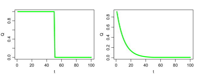
Figure 1: Examples of optimal Q-functions at a given state-action pair with an abrupt change point (left panel) and a gradual change point (right panel).

Algorithm 1 Testing Stationarity for the Optimal Q-Function.

0:  

Input:

The data $\{(S_{i,t},A_{i,t},R_{i,t})\}_{1\leq i\leq N,T_{0}\leq t\leq T}$, and the significance level $0<\alpha<1$.

Step 1.

For each $T_{0}+\epsilon T\leq u\leq(1-\epsilon)T$, employ the gradient Q-learning or fitted Q-iteration algorithm to compute an estimated Q-function $\widehat{Q}_{[T_{0},u]}$ and $\widehat{Q}_{[u,T]}$.

Step 2.

Construct the CUSUM-type test statistics $\textrm{TS}_{1}$, $\textrm{TS}_{\infty}$ or $\textrm{TS}_{n,\infty}$, according to (7), (8) and (9).

Step 3.

Employ multiplier bootstrap to compute the bootstrapped test statistic $\textrm{TS}_{1}^{b}$, $\textrm{TS}_{\infty}^{b}$ or $\textrm{TS}_{n,\infty}^{b}$. Calculate the p-value according to (12).

Output:

Reject the null hypothesis if the $p$-value is smaller than $\alpha$.

3.1 The Main Idea

We focus on the null hypothesis that $Q_{t}^{\tiny{opt}}=Q^{\tiny{opt}}$ for any $t\in\{T_{0},T_{0}+1,\cdots,T\}$ and some integer $T_{0}<T$. We propose an integral-type and two maximum-type test statistics. All test statistics require to estimate the optimal Q-function. First, we propose to use series/sieve method to model $Q^{\tiny{opt}}$. There are two major advantages of using the sieve method here. First, it ensures the resulting Q-estimator has a tractable limiting distribution (see e.g., Theorem 3), which in turn enables us to derive the asymptotic distribution of the test statistic. Second, the number of sieves (e.g., basis functions) is allowed to diverge with the sample size, alleviating the bias resulting from model misspecification.

Specifically, we propose to model $Q^{\tiny{opt}}(a,s)$ by $\phi_{L}^{\top}(a,s)\beta^{*}$ for some $\beta^{*}\in\mathbb{R}^{L}$ where $\phi_{L}(a,s)$ denotes a vector consisting of $L$ basis functions. In the tabular case where both the state and the action spaces are discrete, one could use a lookup table and set

$$\phi_{L}(a,s)=[\mathbb{I}\{(a,s)=(a_{1},s_{1})\},\cdots,\mathbb{I}\{(a,s)=(a_{L},s_{L})\}]^{\top}$$

where $\{(a_{j},s_{j})\}_{j}$ correspond to the set consisting all possible action-state pairs. In the case where the action space is discrete and the state space is continuous, we recommend to set

$$\phi_{L}(a,s)=[\mathbb{I}(a=a_{1})\Phi^{\top}(s),\cdots,\mathbb{I}(a=a_{m})\Phi^{\top}(s)]^{\top},$$ (5)

where $\{a_{j}\}_{j}$ corresponds to the action space and $\Phi$ denotes some set of basis functions on the state space, such as power series, Fourier series, splines or wavelets (see e.g., Judd,, 1998). Our practical implementation uses the random Fourier features; see Section 6.1 for details. As we have commented in the introduction, if the transition and reward functions are stationary over time, the proposed test controls the type-I error even when the approximation error decays at a rate that is slower than $O\{(NT)^{-1/2}\}$. This implies that the proposed test will not be overly sensitive to the choice of the number of basis functions and “undersmoothing” (e.g., including sufficient many basis functions such that the squared bias of the estimator shrinks faster than its variance) is not required to guarantee its validity. In practice, we could employ cross validation to determine the number of basis functions; see Section 3.2 for details. However, the smaller the approximation error, the higher the power.

Second, for any time interval $[T_{1},T_{2}]\subseteq[T_{0},T]$ with $T_{1}=T_{0}$ or $T_{2}=T$, we compute the estimator $\widehat{\beta}_{[T_{1},T_{2}]}$ for $\beta^{*}$ using data collected from this interval. A key observation is that, when $Q^{\tiny{opt}}(a,s)=\phi_{L}^{\top}(a,s)\beta^{*}$, it follows from the Bellman optimality equation (4) that $\beta^{*}$ satisfies the following equation:

$${\mathbb{E}}\phi_{L}(A_{t},S_{t})\left\{R_{t}+\gamma\max_{a}\beta^{*\top}\phi_{L}(a,S_{t+1})-\beta^{*\top}\phi_{L}(A_{t},S_{t})\right\}=0.$$

This motivates us to compute $\widehat{\beta}_{[T_{1},T_{2}]}$ by solving the following estimating equation,

$$\sum_{i=1}^{N}\sum_{t=T_{1}}^{T_{2}-1}\phi_{L}(A_{i,t},S_{i,t})\left\{R_{i,t}+\gamma\max_{a}\beta^{\top}\phi_{L}(a,S_{i,t+1})-\beta^{\top}\phi_{L}(A_{i,t},S_{i,t})\right\}=0.$$ (6)

Under the null hypothesis, it follows from (4) that the left-hand-side (LHS) has zero mean when $\beta=\beta^{*}$. Consequently, the above estimating equation is consistent. However, it remains challenging to compute $\widehat{\beta}_{[T_{1},T_{2}]}$ due to the existence of the non-smooth max operator in the curly brackets. In practice, we could either employ the gradient Q-learning algorithm or the fitted Q-iteration algorithm to solve the estimating equation. See Section 3.2 for more details. Based on this estimator, we formally define the estimated Q-function $\widehat{Q}_{[T_{1},T_{2}]}(a,s)$ as $\phi_{L}^{\top}(a,s)\widehat{\beta}_{[T_{1},T_{2}]}$.

Third, for any candidate change point $T_{0}+\epsilon T\leq u\leq(1-\epsilon)T$, we use $\widehat{Q}_{[u,T]}(a,s)-\widehat{Q}_{[T_{0},u-1]}(a,s)=\phi_{L}^{\top}(a,s)(\widehat{\beta}_{[u,T]}-\widehat{\beta}_{[T_{0},u-1]})$ to measure the difference in the optimal Q-function before and after the change point. Based on this measure, we propose an $\ell_{1}$-type, a maximum-type test statistic, and a normalized maximum-type test statistic, given by

(7)

$$\textrm{TS}_{1}=\max_{T_{0}+\epsilon T<u<(1-\epsilon)T}\sqrt{\frac{(u-T_{0})(T-u)}{(T-T_{0})^{2}}}\left\{\frac{1}{NT}\sum_{i,t}|\widehat{Q}_{[T_{0},u]}(A_{i,t},S_{i,t})-\widehat{Q}_{[u,T]}(A_{i,t},S_{i,t})|\right\},$$

$$\textrm{TS}_{\infty}=\max_{T_{0}+\epsilon T<u<(1-\epsilon)T}\max_{a,s}\sqrt{\frac{(u-T_{0})(T-u)}{(T-T_{0})^{2}}}|\widehat{Q}_{[T_{0},u]}(a,s)-\widehat{Q}_{[u,T]}(a,s)|,$$ (8)

$$\textrm{TS}_{n}=\max_{T_{0}+\epsilon T<u<(1-\epsilon)T}\max_{a,s}\sqrt{\frac{(u-T_{0})(T-u)}{(T-T_{0})^{2}}}\widehat{\sigma}^{-1}_{u}(a,s)|\widehat{Q}_{[T_{0},u]}(a,s)-\widehat{Q}_{[u,T]}(a,s)|,$$ (9)

respectively, where $\widehat{\sigma}^{2}_{u}(a,s)$ denotes some consistent variance estimator of $\widehat{Q}_{[T_{0},u]}(a,s)-\widehat{Q}_{[u,T]}(a,s)$ whose detailed form is given in Appendix B.1.2 of the supplementary article.

We make a few remarks. First, the three test statistics are very similar to the classical cumulative sum (CUSUM) statistic in change point analysis (Csörgö et al.,, 1997). According to the weight scale $\sqrt{u(\kappa-u)/\kappa}$, both test statistics assign less weights on the boundary data points. In addition, $\epsilon$ denotes some user-specified boundary cut-off parameter. Removing the boundary points is necessary as it is difficult to estimate the Q-function that is close to the endpoints. Such practice is commonly employed in the time series literature for change point detection in non-Gaussian settings (see e.g., Cho and Fryzlewicz,, 2012; Yu and Chen,, 2021).

Second, the three test statistics differ in the ways they aggregate the estimated changes $|\widehat{Q}_{[T_{0},u]}-\widehat{Q}_{[u,T]}|$ over different state-action pairs. The $\ell_{1}$-type test averages the changes with weights assigned according to the empirical state-action distribution whereas the two maximum-type tests focuses on the largest change in the (normalized) absolute value. Among the two maximum-type test statistics, the normalized test can be more efficient. This is because when $\widehat{Q}_{[T_{0},u]}(a,s)-\widehat{Q}_{[u,T]}(a,s)$ is not consistent for some value of $(a,s)$, the argmax $\operatorname*{arg\,max}_{a,s}|\widehat{Q}_{[T_{0},u]}(a,s)-\widehat{Q}_{[u,T]}(a,s)|$ might differ significant from the oracle maximiser $\operatorname*{arg\,max}_{a,s}|Q^{\tiny{opt}}_{[T_{0},u]}(a,s)-Q^{\tiny{opt}}_{[u,T]}(a,s)|$, thus lowering the power of the unnormalized test. The normalized test alleviates this issue by taking standard errors of these estimators into consideration. For state-action pairs with inconsistent Q-values, their differences $\widehat{Q}_{[T_{0},u]}-\widehat{Q}_{[u,T]}$ would have large standard errors. As such, those pairs are unlikely to be the argmax. In addition, the normalized test requires a weaker condition to control the type-I error. See Section 5 for details. We also remark that the studentised supremum type statistics have been used in the economics literature (see e.g., Belloni et al.,, 2015; Chen and Christensen,, 2015, 2018).

Finally, we develop a bootstrap-based procedure to compute the critical values for $\textrm{TS}_{1}$, $\textrm{TS}_{\infty}$ and $\textrm{TS}_{n}$. As we will show in Section A, each estimator $\widehat{\beta}_{[T_{1},T_{2}]}$ computed by solving (6) is asymptotically normal. As such, the estimated Q-function is asymptotically normal as well. This motivates us to do employ the multiplier bootstrap to approximate the asymptotic distribution of the Q-estimator and the resulting test statistics. The p-value is obtained based on the empirical distribution of the bootstrap samples. See Section 3.3 for details. Under a given significance level $\alpha$, we reject the test when the p-value is smaller than $\alpha$.

3.2 Estimation of the Q-Function

There are multiple estimation methods available to compute $\widehat{\beta}_{[T_{1},T_{2}]}$ that satisfies the estimating equation (6). We employ the fitted Q-iteration (FQI) algorithm in our implementation. Meanwhile, other methods such as the greedy gradient Q-learning algorithm (Maei et al.,, 2010; Ertefaie and Strawderman,, 2018) are equally applicable. Statistical properties of the estimated Q-function based on FQI are discussed in Appendix A.

The main idea of FQI is to iteratively update the Q-function based on the Bellman optimality equation. During each iteration, it computes $Q^{(k+1)}$ by minimizing

$$Q^{(k+1)}=\operatorname*{arg\,min}_{Q}\sum_{i,t}\left\{R_{i,t}+\gamma\max_{a}Q^{(k)}(a,S_{i,t+1})-Q(A_{i,t},S_{i,t})\right\}^{2}.$$

The above optimization can be cast into a supervised learning problem with $\{R_{i,t}+\gamma\max_{a}Q^{(k)}(a,S_{i,t+1})\}_{i,t}$ as the responses and $\{(A_{i,t},S_{i,t})\}_{i,t}$ as the predictors. When a linear sieve model is imposed for the optimal Q-function, the estimator $\widehat{\beta}_{[T_{1},T_{2}]}$ can be iteratively updated using ordinary least-square regression (OLS). In Section A, we show that such an algorithm converges in the sense that the resulting estimator solves the estimating equation in (6), and derive the asymptotic distribution of $\widehat{\beta}_{[T_{1},T_{2}]}$.

3.3 Bootstrap for P-Value

We develop a multiplier bootstrap method to obtain the p-values. The idea is to generate bootstrap samples to approximate the limiting distribution of $\textrm{TS}_{1}$, $\textrm{TS}_{\infty}$ and $\textrm{TS}_{n}$, defined in (7)-(9), respectively. A key observation is that, under the null hypothesis, when the Q-function is well-approximated and the optimal policy is uniquely defined, the estimated Q-function $\phi(a,s)^{\top}\widehat{\beta}_{[T_{1},T_{2}]}$ has the following linear representation:

$$\begin{split}&\phi(a,s)\widehat{\beta}_{[T_{1},T_{2}]}-Q^{\tiny{opt}}(a,s)\\ =&\frac{1}{N(T_{2}-T_{1})}\phi_{L}^{\top}(a,s)W_{[T_{1},T_{2}]}^{-1}\sum_{i=1}^{N}\sum_{t=T_{1}}^{T_{2}-1}\phi_{L}(A_{i,t},S_{i,t})\delta_{i,t}^{*}+o_{p}(1),\end{split}$$ (10)

where

$$W_{[T_{1},T_{2}]} = \frac{1}{T_{2}-T_{1}}\sum_{t=T_{1}}^{T_{2}-1}{\mathbb{E}}\phi_{L}(A_{i,t},S_{i,t})\{\phi_{L}(A_{i,t},S_{i,t})-\gamma\phi_{L}(\pi^{\tiny{opt}}(S_{i,t+1}),S_{i,t+1})\}^{\top},$$

$$\delta_{i,t}^{*} = R_{i,t}+\gamma\max_{a}Q^{\tiny{opt}}(a,S_{i,t+1})-Q^{\tiny{opt}}(A_{i,t},S_{i,t}).$$

We refer to the proof of Theorem 3 in the supplementary article for details. By the Bellman optimality equation, the leading term on the RHS of (10) forms a mean-zero martingale. When its quadratic variation process converges, it follows from the martingale central limit theorem (McLeish,, 1974) that $\widehat{\beta}_{[T_{1},T_{2}]}$ is asymptotically normal.

In addition, it follows from (10) that

$$\begin{aligned} \widehat{Q}_{[T_{0},u]}(a,s)-\widehat{Q}_{[u,T]}(a,s)=\frac{1}{N(u-T_{0})}\phi_{L}^{\top}(a,s)W_{[T_{0},u]}^{-1}\sum_{i=1}^{N}\sum_{t=T_{0}}^{u-1}\phi_{L}(A_{i,t},S_{i,t})\delta_{i,t}^{*}\\ -\frac{1}{N(T-u)}\phi_{L}^{\top}(a,s)W_{[u,T]}^{-1}\sum_{i=1}^{N}\sum_{t=u}^{T-1}\phi_{L}(A_{i,t},S_{i,t})\delta_{i,t}^{*}+o_{p}(1).\end{aligned}$$ (11)

This motivates us to construct bootstrap samples that approximate the asymptotic distribution of the leading term on the RHS of (11). Specifically, at the $b$th iteration, we consider the bootstrap sample $\widehat{Q}^{b}_{[T_{0},u]}(a,s)-\widehat{Q}^{b}_{[u,T]}(a,s)$ where

$$\widehat{Q}^{b}_{[T_{1},T_{2}]}(a,s)=\frac{1}{N(T_{2}-T_{1})}\phi_{L}^{\top}(a,s)\widehat{W}_{[T_{1},T_{2}]}^{-1}\sum_{i=1}^{N}\sum_{t=T_{1}}^{T_{2}-1}\phi_{L}(A_{i,t},S_{i,t})\delta_{i,t}(\widehat{\beta}_{[T_{1},T_{2}]})e_{i,t}^{b},\,\,\,\,\forall T_{1},T_{2},$$

where $\delta_{i,t}(\beta)$ is the temporal difference error

$$\delta_{i,t}(\beta)=R_{i,t}+\gamma\max_{a}\beta^{\top}\phi_{L}(a,S_{i,t+1})-\beta^{\top}\phi_{L}(A_{i,t},S_{i,t}),$$

$\widehat{W}_{[T_{1},T_{2}]}$ denotes some consistent estimator for $W_{[T_{1},T_{2}]}$, defined by

$$\widehat{W}_{[T_{1},T_{2}]}=\frac{1}{N(T_{2}-T_{1})}\sum_{i=1}^{N}\sum_{t=T_{1}}^{T_{2}-1}\phi_{L}(A_{i,t},S_{i,t})\{\phi_{L}(A_{i,t},S_{i,t})-\gamma\phi_{L}(\pi_{\widehat{\beta}_{[T_{1},T_{2}]}}(S_{i,t+1}),S_{i,t+1})\}^{\top},$$

and $\{e_{i,t}^{b}\}_{i,t}$ correspond to a sequence of i.i.d. standard normal random errors that are independent of the observed data. This yields the bootstrapped statistics,

$$\textrm{TS}_{1}^{b}=\max_{T_{0}+\epsilon T<u<(1-\epsilon)T}\sqrt{\frac{(u-T_{0})(T-u)}{(T-T_{0})^{2}}}\left\{\frac{1}{NT}\sum_{i,t}|\widehat{Q}_{[T_{0},u]}^{b}(A_{i,t},S_{i,t})-\widehat{Q}^{b}_{[u,T]}(A_{i,t},S_{i,t})|\right\},$$

$$\textrm{TS}_{\infty}^{b}=\max_{T_{0}+\epsilon T<u<(1-\epsilon)T}\max_{a,s}\sqrt{\frac{(u-T_{0})(T-u)}{(T-T_{0})^{2}}}|\widehat{Q}_{[T_{0},u]}^{b}(a,s)-\widehat{Q}_{[u,T]}^{b}(a,s)|,$$

$$\textrm{TS}_{n,\infty}^{b}=\max_{T_{0}+\epsilon T<u<(1-\epsilon)T}\max_{a,s}\sqrt{\frac{(u-T_{0})(T-u)}{(T-T_{0})^{2}}}\widehat{\sigma}^{-1}_{u}(a,s)|\widehat{Q}_{[T_{0},u]}^{b}(a,s)-\widehat{Q}_{[u,T]}^{b}(a,s)|.$$

In Section 5.2, we show that under the null hypothesis, the asymptotic distributions of $\textrm{TS}_{1}$, $\textrm{TS}_{\infty}$ and $\textrm{TS}_{n,\infty}$ can be well-approximated by the conditional distributions of $\textrm{TS}_{1}^{b}$, $\textrm{TS}_{\infty}^{b}$ and $\textrm{TS}_{n,\infty}^{b}$ given the observed data. The corresponding p-values are given by

$${\mathbb{P}}(\textrm{TS}_{1}^{b}>\textrm{TS}_{1}|\textrm{Data}),\,\,\,\,{\mathbb{P}}(\textrm{TS}_{\infty}^{b}>\textrm{TS}_{\infty}|\textrm{Data})\,\,\hbox{and}\,\,{\mathbb{P}}(\textrm{TS}_{n,\infty}^{b}>\textrm{TS}_{n,\infty}|\textrm{Data})$$ (12)

respectively. We reject the null when the p-value is smaller than a given significance level $\alpha$.

4 Change Point Detection

In this section, we sequentially apply the proposed test for change point detection. We focus on identifying the most recent change point. As commented in the introduction, such a procedure can be naturally coupled with existing RL algorithms for policy learning in nonstationary environments. Specifically, given the offline data collected from $N$ subjects up to time $T$, we aim to learn a “warm-up” optimal policy that can be used for treatment recommendation for these subjects after time $T$. Due to the potential nonstationarity in the data, it is not desirable to apply existing Q-learning type algorithms to all the data. Our solution is to identify the most recent change point $T^{*}$ such that $\{Q^{\tiny{opt}}_{t}\}_{T^{*}\leq t<T}$ are close to $Q^{\tiny{opt}}_{T}$ and apply Q-learning to the data subset $\{(S_{i,t},A_{i,t},R_{i,t})\}_{1\leq i\leq N,T^{*}\leq t\leq T}$. Such a procedure can be sequentially applied for online policy learning as data accumulate. See Section 6 for details.

In the rest of this section, we propose a data-adaptive method to determine $T^{*}$. We begin by specifying a monotonically increasing sequence $\{\kappa_{j}\}_{j}$. We next set $T^{*}$ to be the location whose fitted value is smaller than the nominal level for the first time. If no changes are detected, we propose to use all the observed data for policy optimization.

5 Theory

We prove the consistency of the proposed test procedure in Section 3. We first introduce the technical conditions. We next establish the consistency of the proposed test. To save space, we derive the asymptotic distribution of the Q-function estimator based on FQI in Appendix A. To simplify the theoretical analysis, we focus on the setting where the action space $\mathcal{A}=\{0,1,\cdots,m-1\}$ is discrete with $m$ being the total number of available actions, the state space is continuous, and $\phi_{L}(a,s)=[\mathbb{I}(a=0)\Phi^{\top}(s),\cdots,\mathbb{I}(a=m-1)\Phi^{\top}(s)]^{\top}\in\mathbb{R}^{L}$ for some set of basis functions $\Phi$ on the state space $\mathcal{S}$, such as the tensor product of B-splines or Wavelets (see Section 6 for a review of these basis functions Chen and Christensen,, 2015). Without loss of generality, we assume $\mathcal{S}=[0,1]^{d}$ where $d$ denotes the dimension of the state. This assumption could be relaxed by assuming $\mathcal{S}$ is a compact subset of $\mathbb{R}^{d}$. We use $p_{t}(\bullet|a,s)$ to denote the probability density function of $F_{t}(a,s,\varepsilon)$. In other words, $p_{t}$ corresponds to the density function of $S_{t+1}$ given $(A_{t},S_{t})=(a,s)$. We use $\pi_{t}^{\tiny{opt}}$ to denote the optimal policy that is greedy with respect to $Q_{t}^{\tiny{opt}}$.

As commented in the introduction, all the theories in this section are established under a bidirectional asymptotic framework. They are valid as either $N$ or $T$ diverges to infinity.

5.1 Technical Conditions

For any integers $T_{1},T_{2}\in[T_{0},T]$, to allow for model misspecification, we define the population-level least false parameter $\beta^{*}_{[T_{1},T_{2}]}$ as follows,

(13)

$$\left[\sum_{t=T_{1}}^{T_{2}-1}{\mathbb{E}}\phi_{L}(A_{t},S_{t})\{\phi_{L}(A_{t},S_{t})-\gamma\phi_{L}(\pi^{\tiny{opt}}_{t}(S_{t+1}),S_{t+1})\}^{\top}\right]^{-1}\left\{\sum_{t=T_{1}}^{T_{2}-1}{\mathbb{E}}\phi_{L}(A_{t},S_{t})R_{t}\right\}.$$

We introduce the following conditions. Specifically, (A1) is concerned with the estimated Q-function, (A2) and (A3) are concerned with the system dynamics, (A4)-(A6) are concerned with the basis functions, (A7) and (A8) are concerned with the behavior policy, (A9) and (A10) are concerned with the optimal policy/Q-function.

Estimated Q-function. (A1) When $Q_{t}^{\tiny{opt}}=Q^{\tiny{opt}}$ is stationary for any integer $t\in[T_{1},T_{2}-1]$, $\widehat{\beta}_{[T_{1},T_{2}]}$ (see 6) has the following linear representation:

$$\begin{split}&\widehat{\beta}_{[T_{1},T_{2}]}-\beta^{*}_{[T_{1},T_{2}]}\\ =&\frac{1}{N(T_{2}-T_{1})}W_{[T_{1},T_{2}]}^{-1}\sum_{i=1}^{N}\sum_{t=T_{1}}^{T_{2}-1}\phi_{L}(A_{i,t},S_{i,t})\delta_{i,t}^{*}-b_{[T_{1},T_{2}]}+O(N^{-c_{1}}T^{-c_{1}}),\end{split}$$ (14)

for some constant $c_{1}>1/2$, with probability at least $1-O(N^{-1}T^{-1})$, where the big-$O$ term is uniform in $\{(T_{1},T_{2}):T_{2}-T_{1}\geq\epsilon T\}$ and $b_{[T_{1},T_{2}]}$ is given by

$$\frac{W_{[T_{1},T_{2}]}^{-1}}{T_{2}-T_{1}}\sum_{t=T_{1}}^{T_{2}-1}{\mathbb{E}}\phi_{L}(A_{t},S_{t})[Q^{\tiny{opt}}_{t}(A_{t},S_{t})-\gamma\max_{a}Q^{\tiny{opt}}(a,S_{t+1})-$$

$$\{\phi_{L}(A_{t},S_{t})-\gamma\phi_{L}(\pi_{t}^{\tiny{opt}}(S_{t+1}),S_{t+1})\}^{\top}\beta_{[T_{1},T_{2}]}^{*}].$$

Remark 1.

The first two terms on the right-hand-side (RHS) of (14) characterise the variation and bias of $\widehat{\beta}_{[T_{1},T_{2}]}-\beta^{*}_{[T_{1},T_{2}]}$, respectively. Under settings where $L$ is fixed and the linear model is correctly specified, Ertefaie and Strawderman, (2018) obtained a similar linear representation for $\widehat{\beta}_{[T_{1},T_{2}]}$ computed via the gradient greedy Q-learning algorithm. In Appendix A, we will show that (A1) holds when FQI is used to compute $\widehat{\beta}_{[T_{1},T_{2}]}$.

System dynamics. (A2) $\{p_{t}(s^{\prime}|a,s)\}_{t}$, $\{r_{t}(a,s)\}_{t}$ are $p$-smooth (Hölder smooth) functions of $s$, i.e., $p_{t}(s^{\prime}|a,\bullet),r_{t}(a,\bullet)\in\Lambda(p,c)$ (see the supplementary materials) for some constant $c>0$ and some $p\geq 1$.

(A3) $\sup_{a,t}{\mathbb{E}}\|F_{t}(s,a,\varepsilon_{1})-F_{t}(s^{\prime},a,\varepsilon_{1})\|_{2}\leq\rho\|s-s^{\prime}\|_{2}$ for some $0\leq\rho<1$ and $\sup_{t,a,s}\|F_{t}(s,a,\varepsilon)-F_{t}(s,a,\varepsilon^{\prime})\|_{2}=O(\|\varepsilon-\varepsilon^{\prime}\|_{2})$. Suppose $\varepsilon_{1}$ has sub-exponential tails, i.e., for any $j$, ${\mathbb{E}}|\varepsilon_{1,j}|^{k}\leq k!c_{3}c_{4}^{k-2}$ for some constants $c_{3},c_{4}>0$ where $\varepsilon_{1,j}$ denotes the $j$th element of the vector $\varepsilon_{1}$.

Remark 2.

First, the smoothness conditions in (A2) are commonly imposed in the sieve estimation literature (see e.g. Huang,, 1998; Chen and Christensen,, 2015). These conditions are used to bound the approximation error of the Q-function. When $p$ is an integer, the $p$-smoothness requires a function to have bounded derivatives up to the $p$th order. More generally, the definition of the class of $p$-smooth functions $\Lambda(p,c)$ can be found in the supplementary article. Under (A2), the Q-function at each time is $p$-smooth as a function of the state as well (Fan et al.,, 2020).

Second, condition (A3) is needed to establish concentration inequalities for nonstationary Markov chains (Alquier et al.,, 2019). It allows us to develop a matrix concentration inequalities with nonstationary transition functions, which is needed to prove the validity of the bootstrap method (see Lemma 2 in the supplementary article for details). This assumption is automatically satisfied when the state satisfies a-time-varying AR(1) process:

$$S_{t+1}=\rho_{t}S_{t}+\beta_{t}A_{t}+\varepsilon_{t},$$

for some $\{\rho_{t}\}_{t}$ and $\{\beta_{t}\}$ such that $\sup_{t}|\rho_{t}|<1$, and $\varepsilon_{t}$ has sub-exponential tails. More generally, it also holds when the auto-regressive model is given by

$$S_{t+1}=f_{t}(A_{t},S_{t})+\varepsilon_{t},$$

with $\sup_{a,t}|f_{t}(a,s)-f_{t}(a,s^{\prime})|\leq\rho\|s-s^{\prime}\|_{2}$ for some $\rho<1$. When the transition functions are stationary over time, it essentially requires the Markov chain to possess the exponential forgetting property (Dedecker and Fan,, 2015).

Basis functions. (A4) There exists some constant $c_{2}>1/2$ such that

$$\sup_{f\in\Lambda(p,C)}\inf_{\beta\in\mathbb{R}^{d}}\sup_{s}|\Phi^{\top}(s)\beta-f(s)|=O(L^{-c_{2}}),$$ (15)

where $L$ denotes the number of basis functions.

(A5) $\lambda_{\max}\{\int_{s}\Phi(s)\Phi^{\top}(s)ds\}=O(1)$, $\sup_{s}\|\Phi(s)\|_{1}=O(\sqrt{L})$.

(A6) Suppose $\sup_{s_{1}\neq s_{2}}\{\|\Phi(s_{1})-\Phi(s_{2})\|_{2}/\|s_{1}-s_{2}\|_{2}\}=O(\sqrt{L})$.

Remark 3.

First, condition (A4) essentially requires that the class of $p$-smooth functions could be uniformly approximated by functions that belong to the linear sieve space. It holds for a wide variety of sieve classes. When tensor product polynomial, trigonometric polynomial, B-spline or wavelet bases are employed, (15) is automatically satisfied with $c_{2}=p/d$ (DeVore and Lorentz,, 1993; Huang,, 1998; Chen,, 2007). (A4) thus holds as long as $p>d/2$.

Second, condition (A5) is automatically satisfied when a tensor-product B-spline or wavelet basis is used, where the constituents of the wavelet basis are arranged such that the coarser level basis functions come ahead of the finer level ones. Specifically, the first part of (A4) can be proven based on the proof of Theorem 3.3 of Burman and Chen, (1989) and that of Theorem 5.1 of Chen and Christensen, (2015). The second part of (A5) follows from the fact that the number of nonzero elements in the vector $\Phi(s)$ is bounded by some universal constant and that each of the basis function is uniformly bounded by $O(\sqrt{L})$.

Finally, (A6) is needed to establish the statistical properties of the maximum-type tests, but is not needed for the $\ell_{1}$-type test. It is automatically satisfied when a tensor-product B-spline is used, since each function in the vector $\Phi$ is a Lipschitz continuous function.

Behavior policy. (A7) The data are generated by a Markov policy $\pi^{b}=\{\pi^{b}_{t}\}_{t}$, i.e.,

$${\mathbb{P}}(A_{t}=a|\{S_{j}\}_{j\leq t},\{A_{j}\}_{j<t},\{R_{j}\}_{j<t})=\pi_{t}^{b}(a|S_{t}),\qquad\forall t.$$

(A8) $\lambda_{\min}{\mathbb{E}}[\phi_{L}(A_{t},S_{t})\phi_{L}(A_{t},S_{t})^{\top}-\gamma^{2}\phi_{L}(\pi_{t}^{\tiny{opt}}(S_{t}),S_{t})\phi_{L}^{\top}(\pi_{t}^{\tiny{opt}}(S_{t}),S_{t})]$ is uniformly bounded away from zero for any $t$.

Remark 4.

First, (A7) allows the behavior policy that generates the data to be nonstationary over time. It is automatically satisfied in randomized studies where the behavior policy is usually a constant function of the state. Second, (A8) is commonly imposed in the statistics literature on RL (see e.g., Ertefaie and Strawderman,, 2018; Luckett et al.,, 2020). It is automatically satisfied when the behavior policy that determines $A_{t}$ is $\varepsilon$-greedy with respect to $\pi_{t}^{\tiny{opt}}$ for some $\varepsilon\leq 1-\gamma^{2}$ (Shi et al.,, 2021).

Optimal policy/Q-function. (A9) The optimal policy $\pi^{\tiny{opt}}_{t}$ is unique for any $t$.

(A10) The margin $Q_{t}^{\tiny{opt}}(\pi^{\tiny{opt}}_{t}(s),s)-\max_{a\in\mathcal{A}\setminus\pi^{\tiny{opt}}_{t}(s)}Q_{t}^{\tiny{opt}}(a,s)$ is bounded away from zero, uniformly for any $s$ and $t$.

Remark 5.

First, (A9) is a necessary condition for establishing the limiting distribution of $\widehat{\beta}_{[T_{1},T_{2}]}$. It is imposed in the statistics literature as well (Luckett et al.,, 2020). It is violated in nonregular settings where the optimal policy is not uniquely defined (Chakraborty et al.,, 2013; Luedtke and van der Laan,, 2016; Shi et al., 2020a, ). The proposed method could be further coupled with data splitting to derive a valid test in nonregular settings. However, the resulting test might suffer from a loss of power, due to the use of data splitting. Second, the margin $Q_{t}^{\tiny{opt}}(\pi^{\tiny{opt}}_{t}(s),s)-\max_{a\in\mathcal{A}-\pi^{\tiny{opt}}_{t}(s)}Q_{t}^{\tiny{opt}}(a,s)$ in (A10) measures the difference between the state-action value under the best action and the second best action. (A10) is imposed to simplify the theoretical analysis. It could be potentially relaxed to require the margin to converge to zero at certain rate or to require the probability that the margin approaches zero to decay to zero at certain rate (see e.g., Qian and Murphy,, 2011; Luedtke and van der Laan,, 2016; Shi et al.,, 2021; Hu et al., 2021b, ).

5.2 Consistency of the Test

We derive the size and power properties of the proposed test in this section.

Theorem 1 (Size).

Suppose (A1)-(A5), (A7)-(A10) hold and $L$ is proportional to $(NT)^{c_{5}}$ for some $0<c_{5}<1/4$. Suppose under the null hypothesis, $\max_{a,s,u}|\phi_{L}^{\top}(a,s)(b_{[T_{0},u]}-b_{[u,T]})|=O\{(NT)^{-c_{6}}\}$ and $\max_{a,s,u}\|\phi_{L}^{\top}(a,s)(\beta_{[T_{0},u]}^{*}-\beta_{[u,T]}^{*})\|_{2}=O\{(NT)^{-c_{6}}\}$ for some $c_{6}>1/2$ where $b$ is defined in (A1) and $\beta^{*}$ is defined in (13). Suppose the boundary removal parameter $\epsilon$ is proportional to $\log^{-c_{7}}(NT)$ for some $c_{7}>0$. Then under the null, we have

$$\sup_{z}|{\mathbb{P}}(\sqrt{NT}\textrm{TS}_{1}^{b}\leq z|\textrm{Data})-{\mathbb{P}}(\sqrt{NT}\textrm{TS}_{1}\leq z)|\stackrel{{\scriptstyle p}}{{\to}}0.$$

In addition, suppose (A6) holds. Then

$$\sup_{z}|{\mathbb{P}}(\sqrt{NT}\textrm{TS}_{n}^{b}\leq z|\textrm{Data})-{\mathbb{P}}(\sqrt{NT}\textrm{TS}_{n}\leq z)|\stackrel{{\scriptstyle p}}{{\to}}0.$$

Finally, suppose the constant $c_{1}$ in (A1) satisfies that $(NT)^{2c_{1}-1}\gg L$. Then

$$\sup_{z}|{\mathbb{P}}(\sqrt{NT}\textrm{TS}_{\infty}^{b}\leq z|\textrm{Data})-{\mathbb{P}}(\sqrt{NT}\textrm{TS}_{\infty}\leq z)|\stackrel{{\scriptstyle p}}{{\to}}0,$$

as either $N$ or $T$ approaches to infinity.

Theorem 1 implies that the limiting distribution of the proposed test can be well-approximated by the conditional distribution of the bootstrapped statistic given the data. It in turn implies that the rejection probability of the proposed test approaches to the nominal level as the total number of observations diverges to infinity. As commented in the introduction, the derivation of the consistency of the proposed test is complicated due to that we allow $L$ to grow with the number of observations. To address this challenge, we develop a matrix concentration inequality for nonstationary MDP in Lemma 2.

In the statement of Theorem 1, we require the difference in the approximation error before and after the change point to decay to zero at a rate of $o\{(NT)^{-1/2}\}$. These assumptions are much weaker than requiring the approximation error to be $o\{(NT)^{-1/2}\}$. The latter requires undersmoothing to ensure the bias of the Q-estimator to converge to zero at a faster rate than its standard deviation. To elaborate, notice that when the transition and reward functions are homogeneous over time, we have $b_{[T_{0},u]}=b_{[u,T]}$ and $\beta_{[T_{0},u]}^{*}=\beta_{[u,T]}^{*}$ (see the definitions of $b$ and $\beta^{*}$ in (A1) and (13)). The assumptions in Theorem 1 are automatically satisfied despite that $\phi_{L}^{\top}(a,s)b_{[T_{0},u]}$ and $\phi_{L}^{\top}(a,s)\beta_{[T_{0},u]}^{*}-Q^{\tiny{opt}}(a,s)$ might converge to zero slower than the parametric rate. As such, undersmoothing is not required and the size property of the proposed test is not overly sensitive to choice of the number of basis functions. The reason why the validity of the proposed test requires a weaker assumption on the approximation error is due to the use of CUSUM-type statistics, which perform scaled differencing at each postulated error location, thereby requiring the difference in approximation errors (rather than absolute approximation errors) to be of a certain order.

Comparatively speaking, the $\ell_{1}$-type test requires weaker conditions than the maximum-type tests. Specifically, the $\ell_{1}$-type test only requires the constant $c_{1}$ in (A1) to be larger than $1/2$ whereas the maximum-type test requires $(NT)^{2c_{1}-1}\gg L$. Moreover, both the normalized and unnormalized maximum-type tests require an additional assumption (A6).

We next establish the power property of the proposed test. In our theoretical analysis, we focus on a particular type of alternative hypothesis where there is a single change-point $T^{*}$ such that $Q_{T_{0}}^{\tiny{opt}}=Q_{T_{0}+1}^{\tiny{opt}}=\cdots=Q_{T^{*}-1}^{\tiny{opt}}$ and $Q_{T^{*}}^{\tiny{opt}}=Q_{T^{*}+1}^{\tiny{opt}}=\cdots=Q_{T}^{\tiny{opt}}$. Under the asymptotics $T\to\infty$, we require $T^{*}\to\infty$ as well. We use $\Delta_{1}=T^{-1}\sum_{a}\sum_{t=0}^{T-1}\int_{s}|Q_{T_{0}}^{\tiny{opt}}(a,s)-Q_{T}^{\tiny{opt}}(a,s)|\pi_{t}(a|s)p_{t}^{b}(s)ds$ and $\Delta_{\infty}=\sup_{a,s}|Q_{T_{0}}^{\tiny{opt}}(a,s)-Q_{T}^{\tiny{opt}}(a,s)|$ to characterise the degree of nonstationarity. Specifically, the null holds if $\Delta_{1}$ or $\Delta_{\infty}$ equals zero and the alternative hypothesis holds if $\Delta_{1}$ or $\Delta_{\infty}$ is positive. However, we remark that the proposed test is consistent against more general alternative hypothesis as well. See Section 6 for details. Notice that in the definition of $\Delta_{1}$, we integrate against the observed state-action distribution $T^{-1}\sum_{t=0}^{T-1}\pi_{t}(a|s)p_{t}^{b}(s)$. Alternatively, the reference distribution can be taken for any measure that is absolutely continuous with respect the observed state-action distribution. For any two positive sequences $\{a_{N,T}\}_{N,T}$ and $\{b_{N,T}\}_{N,T}$, the notation $a_{N,T}\gg b_{N,T}$ means that $b_{N,T}/a_{N,T}\to 0$ as $NT\to\infty$.

Theorem 2 (Power).

Suppose (A1)-(A5), (A7)-(A10) hold and $L$ is proportional to $(NT)^{c_{5}}$ for some $0<c_{5}<1/2$. Suppose $T_{0}+\epsilon T<T^{*}<(1-\epsilon)T$ and $\epsilon$ is proportional to $\log^{-c_{7}}(NT)$ for some $c_{7}>0$.

• If $\Delta_{1}\gg\{\sqrt{L(NT)^{-1}\log(NT)}+L^{-c_{2}}\}\log^{c_{7}/2}(NT)$, then the power of the test based on $\textrm{TS}_{1}$ approaches 1, as either $N$ or $T$ diverges to infinity;

• If $\Delta_{\infty}\gg\sqrt{L}\{\sqrt{L(NT)^{-1}\log(NT)}+L^{-c_{2}}\}\log^{c_{7}/2}(NT)$ and (A6) holds, then the power of the test based on $\textrm{TS}_{\infty}$ approaches 1, as either $N$ or $T$ diverges to infinity.

• If $\Delta_{\infty}\gg\{\sqrt{L(NT)^{-1}\log(NT)}+L^{-c_{2}}\}\log^{c_{7}/2}(NT)$ and (A6) holds, then the power of the test based on $\textrm{TS}_{n}$ approaches 1, as either $N$ or $T$ diverges to infinity.

The assumption $T_{0}+\epsilon T<T^{*}<(1-\epsilon)T$ is reasonable as we allow $\epsilon$ to decay to zero as the number of observations grow to infinity. Under the given assumptions, the bias and standard deviation of the Q-function estimator are proportional to $O(\sqrt{L(NT)^{-1}\log(NT)})$ and $O(L^{-c_{2}})$, respectively. The conditions on $\Delta_{1}$ and $\Delta_{\infty}$ essentially require the signal associated with the alternative hypothesis to be much larger than the estimation error. Similar to the findings in Theorem 1, the unnormalized maximum-type test requires a stronger condition on $L$ to detect the alternative hypothesis. To guarantee the proposed test has good power properties, we use cross-validation to select the number of basis functions, as discussed in Section 6.1. This ensures the bias and standard deviation of the Q-function estimator are approximately of the same order of magnitude, thus minimizing the requirements for $\Delta_{1}$ and $\Delta_{\infty}$.

It is worthwhile to mention that establishing the power property of the test requires a less stringent condition on $L$ than deriving the size property. Specifically, we require $L$ to grow at a rate of $o(\sqrt{NT})$ in Theorem 2. In contrast, this condition is strengthened to $L=o(N^{1/4}T^{1/4})$ in Theorem 1.

6 Simulations

In this section, we conduct simulation studies to evaluate the finite sample performance of the proposed methods and compare against common alternatives. In Section 6.1, we detail the implementation the proposed tests (integral, normalized, unnormalized). Section 6.2 presents results based on four generative models with different nonstationarity scenarios (see Table 1). In Section 6.3, we simulate data to mimic data setup in the motivating application of IHS. All simulation results are aggregated over 100 replications.

6.1 Implementation Details

To implement the proposed tests, the boundary removal parameter $\epsilon$ is set to 0.1; 2000 bootstrap samples are generated to compute p-values. In our simulations, the state variables are continuous. The set of basis functions $\phi_{L}$ is selected according to (5). In particular, we set $\Phi$ to the random Fourier features following the Random Kitchen Sinks (RKS) algorithm (Rahimi and Recht,, 2007); we use RBFsampler function from the Python scikit-learn module for implementation. The bandwidth in the radial basis function (RBF) kernel is selected according to the median heuristic (Garreau et al.,, 2017). The number of basis functions in $\Phi$ (denoted by $M=L/m$) is selected via 5-fold cross-validation. Specifically, for each $M$, let $\Phi_{M}$ denote the resulting set of basis functions. We first divide all data trajectories into 5 non-overlapping data subsets with equal sizes. Let $\mathcal{I}_{\ell}$ denote the set of these subsamples, and $\mathcal{I}_{\ell}^{c}$ denote its complement, $\ell=1,2,3,4,5$. For each combination of $\ell$ and $M$, we use FQI to compute an estimated optimal Q-function $\widehat{Q}_{\ell,M}$ by setting $\Phi=\Phi_{M}$, based on the data subsets in $\mathcal{I}_{\ell}^{c}$. We next select $M$ to minimise the FQI objective function,

$$\begin{aligned} &\sum_{\ell=1}^{5}\sum\limits_{\begin{subarray}{c}(i,t)\in\mathcal{I}_{\ell}\end{subarray}}\left\{R_{i,t}+\gamma\max_{a}\widehat{Q}_{\ell,M}(a,S_{i,t+1})-\widehat{Q}_{\ell,M}(A_{i,t},S_{i,t})\right\}^{2}.\end{aligned}$$ (16)

To mitigate the randomness introduced by the random Fourier features, we repeat each test procedure four times with different random seeds. This yields p-values $\{p_{r},r=1,\ldots,4\}$, for each candidate change point. We then employ the method developed by Meinshausen et al., (2009) to combine these p-values by defining

$$p_{0}=\min\left(1,q_{\tau}\left\{\tau^{-1}p_{r},r=1,\ldots,4\right\}\right),$$ (17)

to be the final p-value. Here, $\tau$ is some constant between 0 and 1, and $q_{\tau}$ is the empirical $\tau$-quantile. Compared to using a single set of Fourier features, such an aggregation method reduces the type-I error and increases the power of the resulting test. In our simulations, results hardly change under $\tau=0.05,0.1,0.15,0.2$; hereafter, we report results under $\tau=0.1$.

6.2 Simulation I

In the following, we conduct two sets of simulation studies to a) assess the performance of the proposed offline testing and change point detection methods, and b) demonstrate the usefulness of the proposed method in an online setting as data accumulate.

a. Offline testing and change point detection. We consider four nonstationary data generating mechanisms with one-dimensional states and binary actions where the nonstationarity occurs in either the state transition function or the reward function, as listed in Table 1. Specifically, in the first two scenarios, the transition function $\mathcal{P}_{t}$ is stationary whereas the reward function $r_{t}$ varies over time. The last two scenarios are concerned with stationary reward functions and nonstationary transition functions. For nonstationary functions, both abrupt (e.g., the underlying function is piece-wise constant) and smooth changes are considered. See Appendix C.3 for more details about the true parameters of the transition and reward functions in these four scenarios.

In all settings, we set $T=$100 and simulate the offline data with sample sizes $N=25,100$. The discount factor $\gamma=0.9,0.95$. The true location of the change point $T^{*}$ is set to $50$. We first apply the each of the proposed tests to the time interval $[T-\kappa,T]$ to detect nonstationarity, where $\kappa$ takes value from a equally-spaced sequence between $25$ and $75$ with increments of $5$. According to our true data generating mechanisms, when $\kappa\leq 50$, the null of no change point over $[T-\kappa,T]$ is true; the alternative hypothesis is true if $\kappa>50$. We fix the significance level $\alpha$ to 0.05. The initial state is sampled from a normal random variable with mean zero and variance 0.5. The actions are generated i.i.d. according to a Bernoulli random variable with a success probability of $0.5$.

	State transition function	Reward function
(1)	Time-homogeneous	Piecewise constant
(2)	Time-homogeneous	Smooth
(3)	Piecewise constant	Time-homogeneous
(4)	Smooth	Time-homogeneous

Table 1: Simulation scenarios with different types of nonstationarity in Section 6.2.

Figure 2 shows the empirical rejection probabilities of each proposed test. We summarise our findings here. First, in all settings, each test can properly control the type I error. Second, the power increases with $\kappa$ as a result of more pre-change-point data being included into the interval $[T-\kappa,T]$. It also increases with $N$, demonstrating the consistency of our tests. Third, as expected, gradual changes are more difficult to detect than abrupt changes. Specifically, it can be seen from Figure 2 that when $\kappa=55$, the power of the proposed test with a smooth reward or state transition function is smaller than that with a piecewise constant reward or state transition function. Finally, the normalized and unnormalized type test statistics achieve slightly higher power than the integral type test statistic when $N=25$, whereas the powers of the three tests become comparable when $N=100$. However, the normalized and unnormalized type test statistics are more computationally expensive especially when the dimension of the state is high, since both require to search the maximum over the entire state-action space.

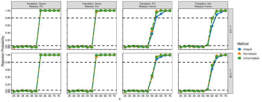
(a) $N=25$.

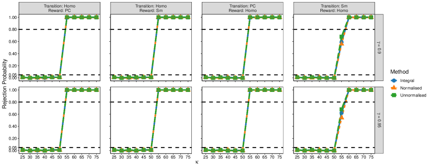
(b) $N=100$.

Figure 2: Empirical type I errors and powers of the proposed test and their associated 95% confidence intervals under settings described in Section 6.2. Abbreviations: Hm for homogeneous, PC for piecewise constant, and Sm for smooth.

Next, we investigate the finite sample performance of the estimated change point location $\widehat{T}^{*}=T-\kappa_{j_{0}-1}$. Figure 3 depicts the histogram of $\widehat{T}^{*}$ in each of the simulation scenarios. It can be seen that in the first two scenarios with abrupt changes, the estimated change points concentrate at $50$, which is the true change point location. In the last two scenarios with smooth changes, the estimated change points have a wider spread when $N=25$, but are still close to 50 in most cases.

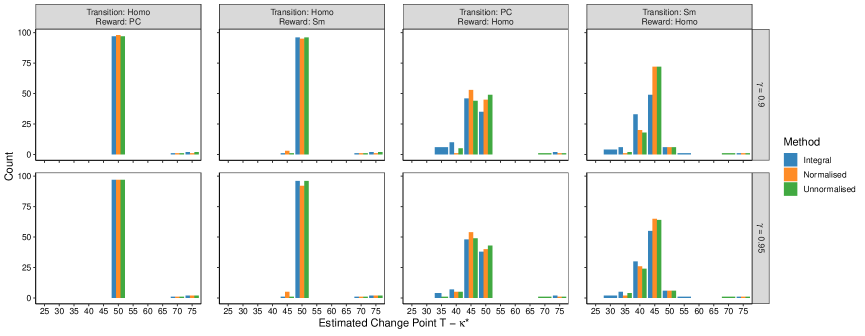
(a) $N=25$.

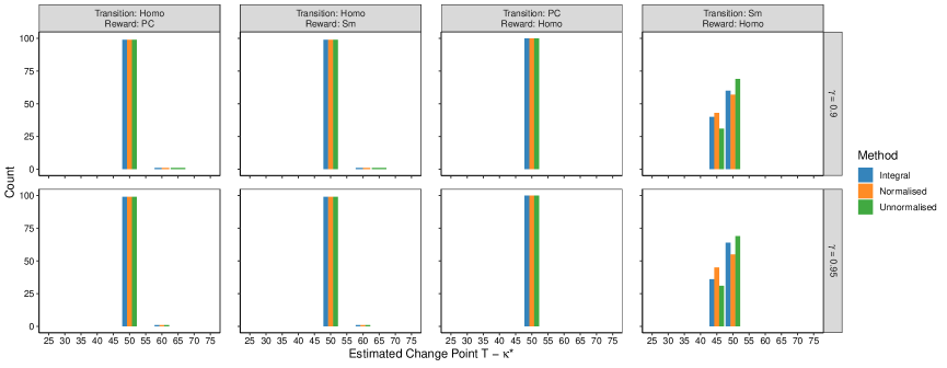
(b) $N=100$.

Figure 3: Distribution of detected change points under simulation settings in Section 6.2.

b. Online value evaluation. Finally, we illustrate how the proposed change point detection method can be coupled with existing state-of-the-art RL algorithms for policy learning in nonstationary environments. In each simulation, we first simulate an offline dataset as discussed earlier with $T=100$ and $N=200$. We next apply our proposal to identify the most recent change point location $\widehat{T}^{*}$ and estimate the optimal policy using the data subset $\{(S_{i,t},R_{i,t},A_{i,t}):1\leq i\leq N,\widehat{T}^{*}\leq t\leq T\}$. As commented earlier, the resulting estimated policy serves as a “warm-up” policy that can be used for treatment recommendation after time $T$. Specifically, we adopt a decision tree model to approximate $Q^{\tiny{opt}}$ to obtain interpretable policies for healthcare researchers. We couple FQI with decision tree regression to compute the Q-estimator $\widehat{Q}$. The decision tree model involves some hyperparameters such as the maximum tree depth and the minimum number of samples on each leaf node. We use 5-fold cross validation to select these hyperparameters from $\{3,5,6\}$ and $\{50,60,80\}$, respectively. See the cross-validation criterion in (16).

Next, for each of the 200 subjects, we use the most recently estimated optimal policy for action selection and data generation, and sequentially apply this procedure for online policy learning as data accumulate to maximize their cumulative reward. Specifically, we consider an online setting and assume the number of change points after $T=100$ follow a Poisson process with rate $1/50$. In other words, we expect a new change point to occur every 50 time points. We set the termination time $T_{end}=300$, yielding 3 to 4 change points in most simulations. We similarly consider four different types of change points listed in Table 1. Whenever a new change point occurs, the effect of the action on the state transition or reward function is reversed. We further consider three different settings with strong, moderate and weak signals by varying the magnitude of treatment effect. For instance, suppose we have two change points $T_{1}$ and $T_{2}$ after $T=100$. In Scenario (1) with a piecewise constant reward function, we set $r(a,s)$ to $1.5\delta as$ when $t\in[100,T_{1})$ or $[T_{2},300]$ and $-1.5\delta as$ when $t\in(T_{1},T_{2}]$ where $\delta$ measures the treatment effect equals $1,0.5$ and $0.2$ in strong-, moderate- and weak-signal settings, respectively.

Finally, we assume that online data come in batches regularly at every $L=25$ time points starting from $T=100$. This yields a total of $K=8$ batches of data. The first data batch is generated according to an $\epsilon$-greedy policy that selects actions using the estimated optimal policy $\widehat{\pi}$ computed based on the data subset in the time interval $[\widehat{T}^{*},T]$ with probability $1-\epsilon$ and a uniformly random policy with probability $\epsilon$. Let $T^{*(0)}=\widehat{T}^{*}$. Suppose we have received $k$ batches of data. We first apply the proposed change point detection method on the data subset in $[T^{*(k-1)},T+kL]$ to identify a new change point $T^{*(k)}$. If no changes are detected, we set $T^{*(k)}=T^{*(k-1)}$. We next update the optimal policy based on the data subset in $[T^{*(k)},T+kL]$ and use this estimated optimal policy (combined with the $\epsilon$-greedy algorithm) to generate the $(k+1)$-th data batch. We repeat this procedure until all 8 batches of data are received. Finally, we aggregate all immediate rewards obtained from time $T$ to $T_{end}$ over the $200$ subjects to estimate the expected return (e.g., average value). Since the proposed three tests yield similar change points and policies, we report the value based on the integral-type test only and compare it against the following baseline methods:

Overall: Standard policy optimization method that uses all the data;
Random: Policy optimization with a randomly assigned change point location;
Kernel: The kernel-based approach developed by Domingues et al., (2021);
Oracle: The “oracle” policy optimization method as if the oracle change point location were known in advance.

For fair comparisons, we use FQI and decision tree regression to compute the optimal Q-function for all competing methods. To implement the random method, after a new batch of data arrives, we randomly pick a time point uniformly from the interval $[T^{*(k-1)},T+kL]$ as the next change point location $T^{*(k)}$ and compute the optimal Q-function based on the observations that occur after time $T^{*(k)}$. To implement the kernel-based method, at the $l$-th FQI iteration, we consider the following objective function,

$$Q^{(l+1)}=\operatorname*{arg\,min}_{Q}\sum_{i,t}K\left(\frac{T-t}{Th}\right)\left\{R_{i,t}+\gamma\max_{a}Q^{(l)}(a,S_{i,t+1})-Q(A_{i,t},S_{i,t})\right\}^{2},$$ (18)

where $K(\cdot)$ denotes the Gaussian RBF basis and $h$ denotes the associated bandwidth parameter taken from the set $\{0,0.1,0.2,0.4,0.8,1.6\}$. According to (18), the kernel-based method assigns larger weights to more recent observations to deal with nonstationarity. After we receive the $k$th data batch, we sample $B\gg T$ data slices across all individuals from $\{(S_{i,t},A_{i,t},R_{i,t},S_{i,t+1};1\leq i\leq N)\}_{0\leq t<T+kL}$ with weights proportional to $K((T-t)/(Th))$ and apply the decision tree regression to these samples to solve (18). To implement the oracle method, we repeatedly use observations that occur after the oracle change point to update the optimal policy.

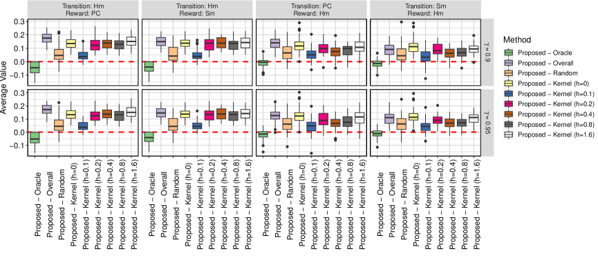
Figure 4: Distribution of the difference between the expected return under the proposed policy and those under policies computed by other baseline methods, under settings in Section 6.2 with strong signal-to-noise ratio. The proposed policy is based on the change point detected by the integral type test statistic. In all scenarios, we find the value results based on the normalized or unnormalized test statistics are similar to those of the integral test statistic.

Figure 4 reports the difference between the proposed policy’s value and values of policies estimated based on these baseline methods in the “strong signal” setting. Additional simulation results with moderate and weak signals in Appendix C.2. We briefly summarize a few notable findings. First, the proposed method achieves much larger policy values compared to the “overall” method, demonstrating the danger of ignoring the nonstationarity. Second, the proposed method is comparable to the oracle method, and outperforms the “random” method in all cases. This implies that correctly identifying the change point location is essential to policy optimization in nonstationary environment. Third, the proposed method is no worse and often better than kernel-based approaches in all cases, again highlighting the necessity of change point detection in policy learning. In addition, as shown in Figure 4, kernel-based method can be sensitive to the choice of the kernel bandwidth and it remains unclear how to determine this tuning parameter in practice.

6.3 Simulation II

To mimic the IHS study, we simulate $N=100$ subjects, each observed over $T=50$ time points. Our aim is to estimate an optimal treatment policy to improve these interns’ long-term physical activity levels. See Section 7 for more details about the study background. At time $t$, the state vector $S_{i,t}$ comprises four variables to mimic the actual IHS study: the square root of step count at time $t$ ($S_{i,t,1}$), cubic root of sleep minutes at time $t$ ($S_{i,t,2}$), mood score at time $t$ ($S_{i,t,3}$), and the square root of step count at time $t-1$ ($S_{i,t,4}=S_{i,t-1,1}$), i.e., the state transition is designed to follow an AR(2) process. See Supplementary C.3 for the true parameter values that govern the dynamics. The actions are binary with $P(A_{it}=1)=0.25$; $A_{it}=1$ means the subject is randomized to receive activity messages at time $t$, and $A_{it}=0$ means any other types of messages or no message at all. Reward $R_{i,t}=S_{i,t,1}$ is defined as the step count at time $t$. We assume that the state transition function has a change point at time $T^{*}=25$. Under this setting, the state transition function is nonstationary whereas the reward is a stationary function of the state. In addition, the data follow the null hypothesis when $\kappa=1,\ldots,25$ and follow the alternative hypothesis for $\kappa=26,\ldots,49$. The discount factor is set to $\gamma=0.9$ or $0.95$. We test the null hypothesis along a sequence of $\kappa=10,15,\ldots,40$ for every five time points. The number of basis $M$ is chosen among $\{10,15,20,25,30\}$.

Figure 5 shows the empirical rejection rates of the proposed tests as well as the distribution of the estimated change point location. Similar to the results in Section 6.2, our proposed tests control the type I error at the nominal level (see $\kappa<25$) and is powerful to detect the alternative hypothesis (see $\kappa>25$). At the boundary where $\kappa=25$ however, the proposed test fails to control the type-I error. Nonetheless, the proposed procedure yields a much better policy compared to the overall and random methods, as we show below. We also remark that the reason the proposed test fails at the boundary is because the marginal distribution of the first few states after the change point is very different from the stationary state distribution. After an initial burn-in period of 5 points, the proposed test is able to control the type-I error at $\kappa=20$. In addition, the distribution of the estimated change point concentrates on $30$, which is very close to the oracle change point location $25$, implying the consistency of the proposed change point detection procedure. We remark that consistency here requires $T^{-1}|\widehat{T}^{*}-T^{*}|\stackrel{{\scriptstyle P}}{{\to}}0$ instead of ${\mathbb{P}}(\widehat{T}^{*}=T^{*})\to 1$, the latter being usually impossible to achieve in change-point settings.

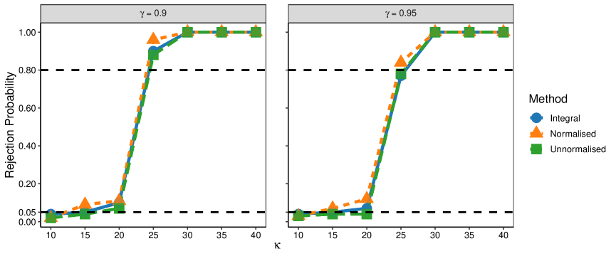
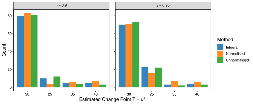
(a) Type I error ($\kappa\leq 25$) and power ($\kappa>25$) .

(b) Estimated change point $\widehat{T}^{*}=T-\kappa_{j_{0}-1}$ where the first rejection occurred at $\kappa_{j_{0}}$.

Figure 5: Simulation II: Empirical rejection rates of the proposed tests (integeral, normalized, and unnormalized) and the distribution of the estimated change points.

7 Application to Intern Health Study

The 2018 Intern Health Study (IHS) is a micro-randomized trial (MRT) that seeks to evaluate the efficacy of push notifications sent via a customised study App upon proximal physical and mental health outcomes (NeCamp et al.,, 2020), a critical first step for designing effective just-in-time adaptive interventions. Over the $26$ weeks, each study subject was re-randomized weekly to receive or not to receive activity suggestions; daily self-reported mood scores were assessed via ecological momentary assessments; step count and sleep duration in minutes were measured by wearables (Fitbit). In this paper, we focus on policy optimization for improving time-discounted cumulative step counts under the infinite horizon setting. However, as have been shown by previous studies (Klasnja et al.,, 2019; Qian et al.,, 2022), subjects may habituate to the prompts or become overburdened, resulting in subjects being less responsive to the contents of the suggestions over time. The treatment effect of activity suggestions may transition from positive to negative, suggesting treatment policies may benefit from adaptation over time. Failure to recognise potential nonstationarity in treatment effects over time may lead to suboptimal policies that overburden subjects, resulting in app deletion and study dropouts. Here we demonstrate how to use the proposed method to detect change point and perform optimal policy estimation in the presence of potential temporal nonstationarity.

7.1 Data and method: Setup

Let the state vector $S_{t}$ be comprised of the following: square root of average step count in week $t$, cubic root of average sleep minutes in week $t$, average mood score in week $t$, and square root of average step count in week $t-1$; all state variables are normalized after respective transformations (NeCamp et al.,, 2020). The reward $R_{t}$ is defined as the average step count in week $t$. The binary action $A_{t}=1$ ($0$) corresponds to pushing (not pushing) an activity message in week $t$. The randomization probabilities are known under MRT: ${\mathbb{P}}(A_{t}=1)=1-{\mathbb{P}}(A_{t}=0)=1/4$. To resemble a real-time evaluation scenario, we divide the data of 26 weeks into two trunks: we perform change point detection and estimate the optimal policy based on data collected in the first $T=22$ weeks (training data batch), and then evaluate the estimated policy on data in the remaining 4 weeks (testing data batch). To implement change point detection, we set $\epsilon=0.08$ and search for change points within $[5,18]$. The number of random Fourier features $M\in\{3,5,8,10\}$ is selected via 5-fold cross validation (see Section 6.1 for implementation details). We repeat this procedure for 20 random seeds and aggregate the produced p-values according to (17). We focus on three specialties: emergency ($N=141$), pediatrics ($N=211$), and family practice ($N=125$). One consideration is that work schedules and activity levels vary greatly across different specialties, and thus medical interns might experience distinct change points. Stratification by specialty may improve homogeneity of the study groups so that the assumption of a common change point is more plausible.

7.2 Results

Figure 6 plots the trajectories of p-values using integral type test statistic; the results are similar when normalized and unnormalized tests were applied to the data (not reported here). We consider $\gamma=0.9$ or $0.95$, which produce similar results. First, we notice that in the pediatrics and family practice specialties, many p-values are close to 1. This is due to the use of the aggregation method in (17) with $r=20$, which tends to increase insignificant p-values and reduce the type-I error. Second, the emergency specialty displays roughly monotonically decreasing p-values over time, whereas at the largest few $\kappa$ values the p-values rise up due to the limited effective sample size at the boundary. Third, the U-shaped p-value trajectory of the pediatrics specialty shows evidence for multiple change points. Specifically, when only a single change point exists, the significant p-values are likely to decrease with $\kappa$. The U-shaped p-value trajectory can occur only when the data interval contains at least two change points and the system dynamics after the second change point is similar to that before the first change occurs, yielding a small CUSUM statistics. Because we focus on the latest detected change point (first $\kappa_{j_{0}-1}$ where $\kappa_{j_{0}}$ results in a rejection of the null) to inform the latest data segment to use for optimal policy estimation, we set $\kappa_{j_{0}-1}=6$ for the emergency specialty and $\kappa_{j_{0}-1}=5$ for the pediatrics specialty, for both choices of $\gamma$. Fourth, the p-value trajectories of the family practice specialty are above the significance threshold (mostly close to 1), indicating the stationarity assumption is compatible with this data subset. We therefore estimate the optimal policy using data from all the time points for family practice specialty.

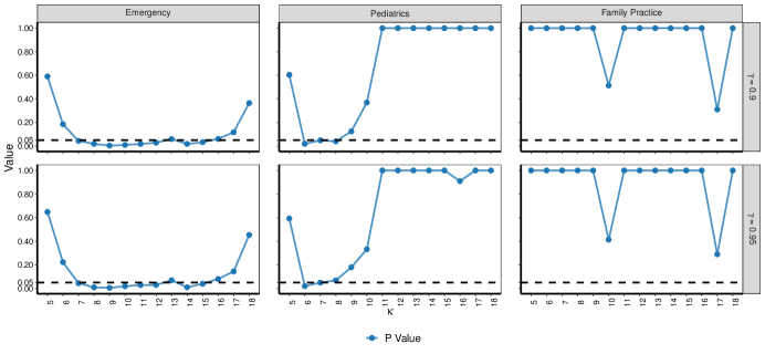
Figure 6: P-values over different values of $\kappa$ (the number of time points from the last time point $T$) under $\gamma=0.9$ (top) and $0.95$ (bottom). The specialties are emergency (left), pediatrics (middle) and family practice (right).

We next compare the proposed policy optimization method with three other methods: 1) overall, 2) random, which were described in Section 6.2) and 3) behavioral, which is the treatment policy used in the completed MRT. The data of the first 22 weeks are used to learn an optimal policy $\widehat{\pi}^{opt}$ through FQI and decision tree regression. In particular, the proposed method uses data after the estimated change point location whereas the overall method uses all the training data. Similar to simulations, hyperparameters of the decision tree regression are selected via 5-fold cross-validation. Next, based on the evaluation data, we applied fitted-Q evaluation (FQE, Le et al.,, 2019) to the testing data of the remaining 4 weeks to evaluate these estimated optimal policies. Results are reported in Table 2. It can be seen that the proposed method achieves larger values when compared to “random” and “behavioral” in all cases, demonstrating the need for change point detection and data-driven decision making. In the following, we focus on comparing the proposed method against “overall”. In the emergency specialty, the optimal policy estimated using data after the detected change point improves weekly average step count per day by about 130 $\sim$ 170 steps relative to the estimated policy based on the overall method. In the pediatrics specialty, however, the overall method achieves a larger weekly average step count by about 40 $\sim$ 112 steps per day. Recall that the proposed method only uses data on $t\in[T-\kappa_{j_{0}-1},T]=[17,22]$ for policy learning. As commented earlier, there are likely two change points in the pediatrics specialty and according to Fig 6, the system dynamics after the first most recent change point are very similar to those before the second most recent change point. As a result, the overall method pools over more data from similar dynamics, resulting in a better policy. This represents a bias-variance trade-off. In settings with a U-shaped p-value trajectory and the most recent change point is close to the second most recent one, it might be sensible to borrow more information from the historical data. Finally, the proposed and overall methods have equal values in the family practice specialty since no change point is identified.

Number of Change Points	Specialty	Method	$\gamma=0.9$	$\gamma=0.95$
$\geq 1$	Emergency	Proposed	8237.16	8295.99
		Overall	8108.13	8127.55
		Behavior	7823.75	7777.32
		Random	8114.78	8080.27
$\geq 2$	Pediatrics	Proposed	7883.08	7848.57
		Overall	7925.44	7960.12
		Behavior	7730.98	7721.29
		Random	7807.52	7815.30
0	Family Practice	Proposed	8062.50	7983.69
		Overall	8062.50	7983.69
		Behavior	7967.67	7957.24
		Random	7983.52	7969.31

Table 2: Mean value estimates using decision tree in anaylsis of IHS. Values are normalized by multiplying $1-\gamma$. All values are evaluated over 10 splits of data.

8 Discussion

We consider testing stationarity and change point detection based on a pre-collected offline dataset. Meanwhile, our proposal can be adopted for policy learning in nonstationary environments, as shown in the numerical study. Recently, there are some works on online nonstationary RL in the computer science literature (see e.g., Lecarpentier and Rachelson,, 2019; Cheung et al.,, 2020; Fei et al.,, 2020; Xie et al.,, 2021; Wei and Luo,, 2021; Zhong et al.,, 2021). Nonetheless, offline hypothesis testing and change point detection have not been studied in these papers.

This supplement is organised as follows. We begin with a list of commonly used notations in the supplement, and introduce some technical definitions. We next establish the asymptotic normality of the Q-function estimator in Appendix A. In Appendix B, we present the proofs of Theorems 1, 2 and 3. Finally, in Appendix C, we detail the simulation setting and present some additional simulation results.

We introduce the class of $p$-smoothness functions. For a $J$-tuple $\alpha=(\alpha_{1},\dots,\alpha_{J})^{\top}$ of nonnegative integers and a given function $h$ on $\mathcal{S}$, let $D^{\alpha}$ denote the differential operator:

$$D^{\alpha}h(s)=\frac{\partial^{\|\alpha\|_{1}}h(s)}{\partial s_{1}^{\alpha_{1}}\cdots\partial s_{J}^{\alpha_{J}}}.$$

Here, $s_{j}$ denotes the $j$th element of $s$. For any $p>0$, let $\lfloor p\rfloor$ denote the largest integer that is smaller than $p$. The class of $p$-smooth functions is defined as follows:

$$\Lambda(p,c)=\left\{h:\sup_{\|\alpha\|_{1}\leq\lfloor p\rfloor}\sup_{s\in\mathcal{S}}|D^{\alpha}h(s)|\leq c,\sup_{\|\alpha\|_{1}=\lfloor p\rfloor}\sup_{\begin{subarray}{c}s_{1},s_{2}\in\mathcal{S}\\ s_{1}\neq s_{2}\end{subarray}}\frac{|D^{\alpha}h(s_{1})-D^{\alpha}h(s_{2})|}{\|s_{1}-s_{2}\|_{2}^{p-\lfloor p\rfloor}}\leq c\right\},$$

for some constant $c>0$.

Appendix A Asymptotic Properties of the Q-Function Estimator

In this section, we focus on investigating the asymptotic properties of the estimated Q-function computed by FQI.

Theorem 3.

Suppose (A2)-(A5), (A7)-(A10) hold and $L$ is proportional to $(NT)^{c_{5}}$ for some $0<c_{5}<1/2$. Suppose $\epsilon$ is proportional to $\log^{-c_{7}}(NT)$ for some $c_{7}>0$. Consider any fixed interval $[T_{1},T_{2}]$ such that $Q_{T_{1}}^{\tiny{opt}}=Q_{T_{1}+1}^{\tiny{opt}}=\cdots=Q_{T_{2}-1}^{\tiny{opt}}$, we have $p_{T_{1}}^{\tiny{opt}}=p_{T_{1}+1}^{\tiny{opt}}=\cdots=p_{T_{2}-1}^{\tiny{opt}}$ and $r_{T_{1}}^{\tiny{opt}}=r_{T_{1}+1}^{\tiny{opt}}=\cdots=r_{T_{2}-1}^{\tiny{opt}}$. Suppose the maximum number of iterations $K$ in FQI satisfies $\log(NT)\ll K=O(N^{c_{8}}T^{c_{8}})$ for any $c_{8}>0$. Then (A1) is satisfied for sufficiently large $NT$.

We again make a few remarks. First, Theorem 3 implies that the asymptotic linear representation in (A1) holds for the FQI estimator. Under the null hypothesis, it follows from the high-dimensional martingale central limit theorem (Belloni and Oliveira,, 2018) that the set of the estimated Q-functions $\{\widehat{Q}_{[T_{1},T_{2}]}\}_{T_{1},T_{2}}$ are jointly asymptotically normal.

Second, as mentioned in the statement of Theorem 3, we require the transition and reward functions to be stationary over time. This is because FQI iteratively updates the Q-function using supervised learning. In contrast, such a condition is not needed when the gradient Q-learning algorithm is employed to learn the optimal Q-function. However, it is worth mentioning that FQI is much easier to implement in practice, as it suffices to implement OLS during each iteration. It could be further extended to employ more general supervised learning algorithms to fit more complicated nonlinear models (e.g., neural networks).

Finally, as commented in the introduction, most works in the literature focused on establishing non-asymptotic error bounds of the FQI estimator (see e.g., Munos and Szepesvári,, 2008; Chen and Jiang,, 2019; Fan et al.,, 2020; Uehara et al.,, 2021). One exception is given by the paper of Hao et al., (2021) who established the limiting distribution of the fitted Q-evaluation (FQE) estimator. We remark that FQE is very similar to FQI but is designed for the purpose of policy evaluation instead of policy optimisation. To our knowledge, this is the first work that investigates the limiting distribution of the FQI estimator in infinite horizon settings, based on nonparametric sieve regression.

Appendix B Proofs

Throughout the proof, we use $c$, $\bar{c}$, $C$, $\bar{C}$ to denote some generic constants whose values are allowed to vary from place to place. For any two positive sequences $\{a_{N,T}\}_{N,T},\{b_{N,T}\}_{N,T}$, the notation $a_{N,T}\preceq b_{N,T}$ means that there exists some constant $C>0$ such that $a_{N,T}\leq Cb_{N,T}$ for any $N$ and $T$.

B.1 Proof of Theorem 1

We begin by introducing the following auxiliary lemmas. Specifically, Lemma 1 derives the uniform rate of convergence of the estimated Q-function. Lemma 2 provides a uniform upper error bound on $|\widehat{W}_{[T_{1},T_{2}]}-W_{[T_{1},T_{2}]}|$. Without loss of generality, assume $T_{0}=0$. Their proofs are provided in Sections B.2 and B.3, respectively.

Lemma 1.

Under the null hypothesis, there exists some constant $\varepsilon_{0}>0$ such that

$$\sup_{a,s,T_{2}-T_{1}\geq\epsilon T}|\widehat{Q}_{[T_{1},T_{2}]}(a,s)-Q^{{opt}}(a,s)|=O\{(NT)^{-\varepsilon_{0}}\},$$

with probability at least $1-O(N^{-1}T^{-1})$, where $\epsilon$ corresponds to the boundary removal parameter defined in Section 3.1.

Lemma 2.

Under the null hypothesis, there exists some constant $\bar{c}>0$ such that $\|W_{[T_{1},T_{2}]}^{-1}\|_{2}\leq\bar{c}$ and that $\sup_{T_{2}-T_{1}\geq\epsilon T}|\widehat{W}_{[T_{1},T_{2}]}-W_{[T_{1},T_{2}]}|=O\{(\epsilon NT)^{-1/2}\sqrt{L\log(NT)}\}$ with probability at least $1-O(N^{-1}T^{-1})$. Here, $\|W_{[T_{1},T_{2}]}^{-1}\|_{2}$ corresponds to the matrix operator norm of $W_{[T_{1},T_{2}]}^{-1}$.

B.1.1 $\ell_{1}$Type Test

We begin with an outline of the proof of Theorem 1. The proof is divided into four steps.

In Step 1, we show there exist some constants $c,C>0$ such that

$${\mathbb{P}}(|\sqrt{NT}(\textrm{TS}_{1}-\textrm{TS}_{1}^{*})|\leq C(NT)^{-c})\to 1,$$ (19)

where

$$\textrm{TS}_{1}^{*}=\max_{\epsilon T<u<(1-\epsilon)T}\sqrt{\frac{u(T-u)}{T^{2}}}\left\{\frac{1}{T}\sum_{t=0}^{T-1}\sum_{a}\int_{s}|\widehat{Q}_{[0,u]}(a,s)-\widehat{Q}_{[u,T]}(a,s)|\pi^{b}_{t}(a|s)p_{t}^{b}(s)ds\right\},$$

where $p_{t}^{b}$ denotes the marginal distribution of $S_{t}$ under the behavior policy. By definition, $\textrm{TS}_{1}^{*}$ corresponds to a version of $\textrm{TS}_{1}$ by assuming the marginal distribution of the observed state-action pairs is known to us.

In the second step, we define

$$\widehat{Q}^{b,0}_{[T_{1},T_{2}]}(a,s)=\frac{1}{N(T_{2}-T_{1})}\phi_{L}^{\top}(a,s)W_{[T_{1},T_{2}]}^{-1}\sum_{i=1}^{N}\sum_{t=T_{1}}^{T_{2}-1}\phi_{L}(A_{i,t},S_{i,t})\delta_{i,t}(\widehat{\beta}_{[T_{1},T_{2}]})e_{i,t},\,\,\,\,\forall T_{1},T_{2},$$

a version of $\widehat{Q}^{b}_{[T_{1},T_{2}]}(a,s)$ with $\widehat{W}_{[T_{1},T_{2}]}^{-1}$ replaced by its oracle value, and establish a uniform upper error bound for $\max_{i,t,T_{1},T_{2}}|\widehat{Q}_{[T_{1},T_{2}]}^{b}(A_{i,t},S_{i,t})-\widehat{Q}_{[T_{1},T_{2}]}^{b,0}(A_{i,t},S_{i,t})|$. Specifically, we show that there exists some constant $c>0$ such that the uniform upper error bound decays to zero at a rate of $O\{(NT)^{-1/2-c}\}$, with probability approaching 1 (WPA1). By triangle inequality, we can show that

$${\mathbb{P}}(|\sqrt{NT}(\textrm{TS}_{1}^{b}-\textrm{TS}_{1}^{b,0})|\leq C(NT)^{-c})\to 1,$$ (20)

for some constant $C>0$, where

$$\textrm{TS}_{1}^{b,0}=\max_{\epsilon T<u<(1-\epsilon)T}\sqrt{\frac{u(T-u)}{T^{2}}}\left\{\frac{1}{NT}\sum_{t=0}^{T-1}\sum_{i=1}^{N}|\widehat{Q}_{[0,u]}^{b,0}(A_{i,t},S_{i,t})-\widehat{Q}_{[u,T]}^{b,0}(A_{i,t},S_{i,t})|\right\}.$$

Using similar arguments as in the proof of (19) in Step 1 (see Pages 7 – 9), we can show that $|\textrm{TS}_{1}^{b,0}-\textrm{TS}_{1}^{b,*}|$ is upper bounded by $C(NT)^{-c}$ for some $c,C>0$, WPA1, where

$$\textrm{TS}_{1}^{b,*}=\max_{\epsilon T<u<(1-\epsilon)T}\sqrt{\frac{u(T-u)}{T^{2}}}\left\{\frac{1}{T}\sum_{t=0}^{T-1}\sum_{a}\int_{s}|\widehat{Q}_{[0,u]}^{b,0}(a,s)-\widehat{Q}_{[u,T]}^{b,0}(a,s)|\pi^{b}_{t}(a|s)p_{t}^{b}(s)ds\right\}.$$

This together with (20) yields that

$${\mathbb{P}}(|\sqrt{NT}(\textrm{TS}_{1}^{b}-\textrm{TS}_{1}^{b,*})|\leq C(NT)^{-c})\to 1,$$

for some constants $c,C>0$. It also implies that

$${\mathbb{P}}(|\sqrt{NT}(\textrm{TS}_{1}^{b}-\textrm{TS}_{1}^{b,*})|\leq C(NT)^{-c}|\textrm{Data})\stackrel{{\scriptstyle P}}{{\to}}1.$$ (21)

In the third step, we define $\textrm{TS}_{1}^{**}$ to be a version of $\textrm{TS}_{1}^{*}$ with $\widehat{Q}_{[T_{1},T_{2}]}$ replaced by the leading term in Assumption (A1). Similarly, we define $\textrm{TS}_{1}^{b,**}$ to be a version of $\textrm{TS}_{1}^{b,*}$ with $\delta_{i,t}(\widehat{\beta}_{[T_{1},T_{2}]})$ replaced by the oracle value $\delta_{i,t}^{*}$. We will show that

$$\begin{aligned} &{\mathbb{P}}(|\sqrt{NT}(\textrm{TS}_{1}^{*}-\textrm{TS}_{1}^{**})|\leq C(NT)^{-c})\to 1,\\ &{\mathbb{P}}(|\sqrt{NT}(\textrm{TS}_{1}^{b,*}-\textrm{TS}_{1}^{b,**})|\leq C(NT)^{-c}|\textrm{Data})\stackrel{{\scriptstyle P}}{{\to}}1.\end{aligned}$$ (22)

Combining the results in (19)-(22), we have shown that

$$\begin{aligned} &{\mathbb{P}}(|\sqrt{NT}(\textrm{TS}_{1}-\textrm{TS}_{1}^{**})|\leq C(NT)^{-c})\to 1,\\ &{\mathbb{P}}(|\sqrt{NT}(\textrm{TS}_{1}^{b}-\textrm{TS}_{1}^{b,**})|\leq C(NT)^{-c}|\textrm{Data})\stackrel{{\scriptstyle P}}{{\to}}1.\end{aligned}$$ (23)

In the last step, we aim to show the proposed test controls the type-I error. A key step in our proof is to bound the Kolmogorov distance between $\textrm{TS}_{1}^{**}$ and $\textrm{TS}_{1}^{b,**}$. This together with (23) yields the validity of the proposed test. Notice that $\textrm{TS}_{1}^{**}$ can be viewed as a function of the set of mean zero random vectors

$$\left\{Z_{u}\equiv\frac{W_{[0,u]}^{-1}}{Nu}\sum_{i=1}^{N}\sum_{t=0}^{u-1}\phi_{L}(A_{i,t},S_{i,t})\delta_{i,t}^{*}-\frac{W_{[u,T]}^{-1}}{N(T-u)}\sum_{i=1}^{N}\sum_{t=u}^{T-1}\phi_{L}(A_{i,t},S_{i,t})\delta_{i,t}^{*}:u\right\}.$$ (24)

Similarly, $\textrm{TS}_{1}^{b,**}$ can be represented as a function of the bootstrapped samples

$$\left\{Z_{u}^{b}\equiv\frac{W_{[0,u]}^{-1}}{Nu}\sum_{i=1}^{N}\sum_{t=0}^{u-1}\phi_{L}(A_{i,t},S_{i,t})\delta_{i,t}^{*}e_{i,t}-\frac{W_{[u,T]}^{-1}}{N(T-u)}\sum_{i=1}^{N}\sum_{t=u}^{T-1}\phi_{L}(A_{i,t},S_{i,t})\delta_{i,t}^{*}e_{i,t}:u\right\}.$$ (25)

When $T$ and $L$ are fixed, the classical continuous mapping theorem can be applied to establish the weak convergence results. However, in our setting, $L$ needs to diverge with the number of observations to alleviate the model misspecification error. We also allow $T$ to approach infinity. Hence, classical weak convergence results cannot be applied. Toward that end, we establish a nonasymptotic error bound for the Kolmogorov distance as a function of $N,T$ and $L$, and show that this bound decays to zero under the given conditions. The proof is based on the high-dimensional martingale central limit theorem developed by Belloni and Oliveira, (2018).

We next detail the proof for each step.

Step 1. For each $u$, we aim to develop a concentration inequality to bound the difference

$$\begin{aligned} \left|\sqrt{\frac{u(T-u)}{T^{2}}}\left\{\frac{1}{NT}\sum_{t=0}^{T-1}\sum_{i=1}^{N}\sum_{a}\int_{s}[|\widehat{Q}_{[0,u]}(A_{i,t},S_{i,t})-\widehat{Q}_{[u,T]}(A_{i,t},S_{i,t})|\right.\right.\\ -\left.\left.|\widehat{Q}_{[0,u]}(a,s)-\widehat{Q}_{[u,T]}(a,s)|]\pi^{b}_{t}(a|s)p_{t}^{b}(s)ds\right\}\right|.\end{aligned}$$ (26)

In the proof of Lemma 1, we have shown that $\sup_{T_{1},T_{2}}\|\widehat{\beta}_{[T_{1},T_{2}]}-\beta^{*}_{[T_{1},T_{2}]}\|_{2}=O(L^{-c})$ for some constant $c>1/2$, with probability at least $1-O(N^{-1}T^{-1})$.

Define the set $\mathcal{B}_{[T_{1},T_{2}]}(C)=\{\beta\in\mathbb{R}^{L}:\|\beta-\beta_{[T_{1},T_{2}]}^{*}\|_{2}\leq CL^{-c}\}$. It follows that there exists some sufficiently large constant $C>0$ such that $\widehat{\beta}_{[T_{1},T_{2}]}\in\mathcal{B}_{[T_{1},T_{2}]}(C)$ with probability at least $1-O(N^{-1}T^{-1})$. (26) can thus be upper bounded by

$$\sup_{\begin{subarray}{c}\beta_{1}\in\mathcal{B}_{[0,u]}(C)\\ \beta_{2}\in\mathcal{B}_{[u,T]}(C)\end{subarray}}\left|\frac{1}{2NT}\sum_{t=0}^{T-1}\sum_{i=1}^{N}\{|\phi_{L}^{\top}(A_{i,t},S_{i,t})(\beta_{1}-\beta_{2})|-{\mathbb{E}}|\phi_{L}^{\top}(A_{i,t},S_{i,t})(\beta_{1}-\beta_{2})|\}\right|.$$ (27)

The upper bound for (27) can be established using similar arguments as in the proof of Lemma 2. To save space, we only provide a sketch of the proof here. Please refer to the proof of Lemma 2 for details.

Notice that the suprema in (27) are taken with respect to infinitely many $\beta$s. As such, standard concentration inequalities are not applicable to bound (27). Toward that end, we first take an $\varepsilon$-net of $\mathcal{B}_{[0,u]}(C)$ and $\mathcal{B}_{[u,T]}(C)$ for some sufficiently small $\varepsilon>0$, denote by $\mathcal{B}_{[0,u]}^{*}(C)$ and $\mathcal{B}_{[u,T]}^{*}(C)$, respectively, such that for any $\beta\in\mathcal{B}_{[0,u]}(C)$ (or $\mathcal{B}_{[u,T]}(C)$), there exists some $\beta^{*}\in\mathcal{B}_{[0,u]}^{*}(C)$ (or $\mathcal{B}_{[u,T]}^{*}(C)$) that satisfies $\|\beta-\beta^{*}\|_{2}\leq\varepsilon$. The purpose of introducing some an $\varepsilon$-net is to approximate these sets by collections of finitely many $\beta$s so that concentration inequalities are applicable to establish the upper bound. Set $\varepsilon=C(NT)^{-2}L^{-c}$. It follows from Lemma 2.2 of Mendelson et al., (2008) that there exist some $\mathcal{B}_{[0,u]}^{*}(C)$ and $\mathcal{B}_{[u,T]}^{*}(C)$ with number of elements upper bounded by $5^{L}(NT)^{2L}$.

Under (A4), we have $\sup_{a,s}\|\phi_{L}(a,s)\|_{2}=O(\sqrt{L})$. Thanks to this uniform bound, the quantity within the absolute value symbol in (27) is a Lipschitz continuous function of $(\beta_{1},\beta_{2})$, with the Lipschitz constant upper bounded by $O(\sqrt{L})$. As such, (27) can be approximated by

$$\sup_{\begin{subarray}{c}\beta_{1}\in\mathcal{B}_{[0,u]}^{*}(C)\\ \beta_{2}\in\mathcal{B}_{[u,T]}^{*}(C)\end{subarray}}\Bigg{|}\underbrace{\frac{1}{2NT}\sum_{t=0}^{T-1}\sum_{i=1}^{N}\sum_{a}\{|\phi_{L}^{\top}(A_{i,t},S_{i,t})(\beta_{1}-\beta_{2})|-{\mathbb{E}}|\phi_{L}^{\top}(A_{i,t},S_{i,t})(\beta_{1}-\beta_{2})|\}}_{I(\beta_{1},\beta_{2})~{}~{}(\textrm{without~{}absolute~{}value})}\Bigg{|},$$ (28)

with the approximation error given by $O(C\sqrt{L}N^{-2}T^{-2}L^{-c})$ where the big-$O$ term is uniform in $u$.

It remains to develop a concentration inequality for (28). Since the number of elements in $\mathcal{B}_{[0,u]}^{*}(C)$ and $\mathcal{B}_{[u,T]}^{*}(C)$ are bounded, we could develop a tail inequality for the quantity within the absolute value symbol in (28) for each combination of $\beta_{1}$ and $\beta_{2}$, and then apply Bonferroni inequality to establish a uniform upper error bound. More specifically, for each pair $(\beta_{1},\beta_{2})$, let

$$I^{*}(\beta_{1},\beta_{2})=\frac{1}{2N\sqrt{T}}\sum_{t=0}^{T-1}\sum_{i=1}^{N}[{\mathbb{E}}\{|\phi_{L}^{\top}(A_{i,t},S_{i,t})(\beta_{1}-\beta_{2})||S_{i,t-1}\}-{\mathbb{E}}|\phi_{L}^{\top}(A_{i,t},S_{i,t})(\beta_{1}-\beta_{2})|],$$

with the convention that $S_{i,-1}=\emptyset$. Notice that $I(\beta_{1},\beta_{2})-I^{*}(\beta_{1},\beta_{2})$ forms a mean-zero martingale under the Markov assumption, we can first apply the martingale concentration inequality (see e.g., Tropp,, 2011) to show that

$$|I(\beta_{1},\beta_{2})-I^{*}(\beta_{1},\beta_{2})|=O(L^{-\varepsilon_{0}}\sqrt{N^{-1}T^{-1}\log(NT)}),$$ (29)

for some $\varepsilon_{0}>0$, with probability at least $1-O\{(NT)^{-CL}\}$ for some sufficiently large constant $C>0$. Here, the upper bound $O(L^{-\varepsilon_{0}}\sqrt{N^{-1}T^{-1}\log(NT)})$ decays faster than the parametric rate, due to the fact that the variance of the summand decays to zero under the condition that $\sup_{a,s,u}|\phi_{L}^{\top}(a,s)(\beta_{[0,u]}^{*}-\beta_{[u,T]}^{*})|=O(N^{-c_{6}}T^{-c_{6}})$ for some $c_{6}>1/2$, imposed in the statement of Theorem 1. Specifically, notice that ${\mbox{Var}}\{\phi_{L}^{\top}(A_{t},S_{t})(\beta_{1}-\beta_{2})|S_{t-1}\}$ is upper bounded by

$${\mathbb{E}}[\{\phi_{L}^{\top}(A_{t},S_{t})(\beta_{1}-\beta_{2})\}^{2}|S_{t-1}]\leq 3{\mathbb{E}}[\{\phi_{L}^{\top}(A_{t},S_{t})(\beta_{[0,u]}^{*}-\beta_{[u,T]}^{*})\}^{2}|S_{t-1}]$$

$$+3{\mathbb{E}}[\{\phi_{L}^{\top}(A_{t},S_{t})(\beta_{1}-\beta_{[0,u]}^{*})\}^{2}|S_{t-1}]+3{\mathbb{E}}[\{\phi_{L}^{\top}(A_{t},S_{t})(\beta_{2}-\beta_{[u,T]}^{*})\}^{2}|S_{t-1}]\leq C(NT)^{-2c_{6}}$$

$$+C\max_{a,a^{\prime},s}\lambda_{\max}\left\{\int_{s^{\prime}}\phi_{L}(a^{\prime},s^{\prime})\phi_{L}^{\top}(a^{\prime},s^{\prime})p(s^{\prime}|a,s)ds^{\prime}\right\}\max(\|\beta_{1}-\beta_{[0,u]}^{*}\|_{2}^{2},\|\beta_{2}-\beta_{[u,T]}^{*}\|_{2}^{2})$$

$$=O(NT)^{-2c_{6}}+O\{\max(\|\beta_{1}-\beta_{[0,u]}^{*}\|_{2}^{2},\|\beta_{2}-\beta_{[u,T]}^{*}\|_{2}^{2})\}=O(NT)^{-2c_{6}}+O(L^{-2c}),$$

for some constant $C>0$, where the first inequality is due to Cauchy-Schwarz inequality, the second inequality is due to the condition on $\sup_{a,s,u}|\phi_{L}^{\top}(a,s)(\beta_{[0,u]}^{*}-\beta_{[u,T]}^{*})|$, and the first equality is due to (A5) and the fact that $p$ is uniformly bounded (see (A2) and the definition of the $p$-smoothness function class).

Next, under (A3), the transition functions $\{F_{t}\}_{t}$ satisfies the conditions in the statement of Theorem 3.1 in Alquier et al., (2019). In addition, under (A5) and the condition that $\sup_{a,s,u}|\phi_{L}^{\top}(a,s)(\beta^{*}_{[0,u]}-\beta^{*}_{[u,T]})|=O\{(NT)^{-c_{6}}\}$ for some $c_{6}>1/2$, each summand in the definition of $I^{*}(\beta_{1},\beta_{2})$ is upper bounded by $O(L^{-c})$ for some $c>1/2$. We can apply the concentration inequality for non-stationary Markov chains developed therein to show that $|I^{*}(\beta_{1},\beta_{2})|=O(L^{-\varepsilon_{0}}\sqrt{N^{-1}T^{-1}\log(NT)})$, with probability at least $1-O\{(NT)^{-CL}\}$ for some sufficiently large constant $C>0$. Similarly, the upper bound $O(L^{-\varepsilon_{0}}\sqrt{N^{-1}T^{-1}\log(NT)})$ decays to zero at a rate faster than the parametric rate due to that each summand ${\mathbb{E}}\{|\phi_{L}^{\top}(A_{i,t},S_{i,t})(\beta_{1}-\beta_{2})||S_{i,t-1}\}-{\mathbb{E}}|\phi_{L}^{\top}(A_{i,t},S_{i,t})(\beta_{1}-\beta_{2})|$ is bounded by $O(L^{-\min(c,c_{6})})$. This together with the upper bound for $|I(\beta_{1},\beta_{2})-I^{*}(\beta_{1},\beta_{2})|$ in (29), Bonferroni inequality and the condition that $L$ is proportional to $(NT)^{c_{5}}$ yields the desired uniform upper bound for (28). This completes Step 1 of the proof.

Step 2. By definition $\widehat{Q}_{[T_{1},T_{2}]}^{b,0}(A_{i,t},S_{i,t})-\widehat{Q}_{[T_{1},T_{2}]}^{b}(A_{i,t},S_{i,t})$ is equal to the sum of

$$\frac{1}{N(T_{2}-T_{1})}\phi_{L}^{\top}(A_{i,t},S_{i,t})(\widehat{W}_{[T_{1},T_{2}]}^{-1}-W_{[T_{1},T_{2}]}^{-1})\sum_{i^{\prime}=1}^{N}\sum_{t^{\prime}=T_{1}}^{T_{2}-1}\phi_{L}(A_{i^{\prime},t^{\prime}},S_{i,t})\delta_{i^{\prime},t^{\prime}}(\widehat{\beta}_{[T_{1},T_{2}]})e_{i^{\prime},t^{\prime}}.$$ (30)

and

$$\frac{1}{N(T_{2}-T_{1})}\phi_{L}^{\top}(A_{i,t},S_{i,t})W_{[T_{1},T_{2}]}^{-1}\sum_{i^{\prime}=1}^{N}\sum_{t^{\prime}=T_{1}}^{T_{2}-1}\phi_{L}(A_{i^{\prime},t^{\prime}},S_{i^{\prime},t^{\prime}})(\delta_{i^{\prime},t^{\prime}}(\widehat{\beta}_{[T_{1},T_{2}]})-\delta_{i^{\prime},t^{\prime}}^{*})e_{i^{\prime},t^{\prime}}.$$ (31)

Consider the first term. In Lemma 2, we establish a uniform upper error bound for $\|\widehat{W}_{[T_{1},T_{2}]}-W_{[T_{1},T_{2}]}\|_{2}$ and show that $\|W_{[T_{1},T_{2}]}^{-1}\|_{2}$ is upper bounded by some constant. Using similar arguments in Part 3 of the proof of Lemma 3 in Shi et al., (2021), we can show that $\|\widehat{W}_{[T_{1},T_{2}]}^{-1}-W_{[T_{1},T_{2}]}^{-1}\|_{2}$ is of the same order of magnitude as $\|\widehat{W}_{[T_{1},T_{2}]}-W_{[T_{1},T_{2}]}\|_{2}$. The boundedness assumption of $R_{t}$ implies that the Q-function is bounded. This together with Lemma 1 implies the estimated Q-function is bounded as well, and so is $\delta_{i^{\prime},t^{\prime}}(\widehat{\beta}_{[T_{1},T_{2}]})$. By (A5), the conditional variance of (30) given the data is upper bounded by

$$\frac{CL^{2}}{\epsilon^{2}N^{2}T^{2}}\lambda_{\max}\left\{\frac{1}{N(T_{2}-T_{1})}\sum_{i=1}^{N}\sum_{t=T_{1}}^{T_{2}-1}\phi_{L}(A_{i,t},S_{i,t})\phi_{L}^{\top}(A_{i,t},S_{i,t})\right\}.$$

Similar to Lemma 2, we can show that the maximum eigenvalue of the matrix inside the curly brackets converges to $\lambda_{\max}\{(T_{2}-T_{1})^{-1}\sum_{t=T_{1}}^{T_{2}-1}{\mathbb{E}}\phi_{L}(A_{t},S_{t})\phi_{L}^{\top}(A_{t},S_{t})\}$, which is bounded by some finite constant under (A5). Under the given conditions on $\epsilon$ and $L$, the conditional variance of (30) given the data is of the order $(NT)^{-2c-1}$, for some constant $c>0$, WPA1. Notice that the probability of a standard normal random variable exceeding $z$ is bounded by $\exp(-z^{2}/2)$ for any $z>1$; see e.g., the inequality for the Gaussian Mill’s ratio (Birnbaum,, 1942). Since (30) is a mean-zero Gaussian random variable given the data, it is of the order $O\{(NT)^{-c-1/2}\sqrt{\log(NT)}\}$, with probability at least $1-O\{(NT)^{-C}\}$ for any sufficiently large constant $C>0$. This together with Bonferroni inequality yields the desired uniform upper error bound for the first term. As for the second term, notice that by Lemma 1, the difference $\delta_{i,t}(\widehat{\beta}_{[T_{1},T_{2}]})-\delta_{i,t}^{*}$ decays at a rate of $(NT)^{-c}$ for some constant $c>0$, uniformly in $i,t,T_{1},T_{2}$, WPA1. Based on this result, we can similarly derive the upper error bound for the second term. This completes the proof.

Step 3. By triangle inequality and (A1), the difference $|\textrm{TS}_{1}^{b,*}-\textrm{TS}_{1}^{b,**}|$ can be upper bounded by

$$\max_{\epsilon T<u<(1-\epsilon)T}\frac{1}{2T}\sum_{t=0}^{T-1}\sum_{a}\int_{s}|\phi^{\top}(a,s)(b_{[0,u]}-b_{[u,T]}+O(N^{-c_{1}}T^{-c_{1}}))|\pi_{t}^{b}(a|s)p_{t}^{b}(s)ds$$

$$\leq\max_{\epsilon T<u<(1-\epsilon)T}\frac{1}{2T}\sum_{t=0}^{T-1}\sum_{a}\int_{s}|\phi^{\top}(a,s)(b_{[u,T]}-b_{[0,u]})|\pi_{t}^{b}(a|s)p_{t}^{b}(s)ds$$

$$+O(N^{-c_{1}}T^{-c_{1}})\max_{\epsilon T<u<(1-\epsilon)T}\sup_{\nu\in\mathbb{R}^{L}:\|\nu\|_{2}=1}\frac{1}{2T}\sum_{t=0}^{T-1}\sum_{a}\int_{s}|\phi^{\top}(a,s)\nu|\pi_{t}^{b}(a|s)p_{t}^{b}(s)ds,$$

WPA1. The first term on the RHS is $O\{(NT)^{-c_{6}}\}$ under the given conditions in the statement of Theorem 1. Under (A2), $\{p_{t}\}_{t}$ is uniformly bounded. So is $\{p_{t}^{b}\}_{t}$. It follows from (A5) that the second term is $O(N^{-c_{1}}T^{-c_{1}})$. This yields the first assertion in (22). The second assertion can be similarly proven based on the result $\sup_{T_{1},T_{2}}\|\widehat{\beta}_{[T_{1},T_{2}]}-\beta^{*}_{[T_{1},T_{2}]}\|_{2}=O(L^{-c})$ for some constant $c>1/2$, WPA1, as shown in Lemma 1.

Step 4. As we have commented, the proof is based on the high-dimensional martingale central limit theorem developed by Belloni and Oliveira, (2018). Let $Z$ and $Z^{b}$ denote the high-dimensional random vectors formed by stacking the random vectors in the set (24) and (25), respectively. It can be represented as $\sum_{i,t}Z_{i,t}$ where each $Z_{i,t}$ depends on the data tuple $(S_{i,t},A_{i,t},R_{i,t},S_{i,t+1})$. We first observe that it corresponds to a sum of high-dimensional martingale difference. Specifically, for any integer $1\leq g\leq NT$, let $i(g)$ and $t(g)$ be the quotient and the remainder of $g+T-1$ divided by $T$ that satisfy

$$g=\{i(g)-1\}T+t(g)+1\,\,\,\,\hbox{and}\,\,\,\,0\leq t(g)<T.$$

Let $\mathcal{F}^{(0)}=\{S_{1,0},A_{1,0}\}$. Then we recursively define $\{\mathcal{F}^{(g)}\}_{1\leq g\leq NT}$ as follows:

$$\mathcal{F}^{(g)}=\left\{\begin{array}[]{ll}\mathcal{F}^{(g-1)}\cup\{R_{i(g),t(g)},S_{i(g),t(g)+1},A_{i(g),t(g)+1}\},&\hbox{if}~{}t(g)<T-1;\\ \mathcal{F}^{(g-1)}\cup\{R_{i(g),T-1},S_{i(g),T},S_{i(g)+1,0},A_{i(g)+1,0}\},&\hbox{otherwise}.\end{array}\right.$$

This allows us to rewrite $Z$ as $\sum_{g=1}^{NT}Z^{(g)}=\sum_{g=1}^{NT}Z_{i(g),t(g)}$. Similarly, we can rewrite $Z^{b}$ as $\sum_{g=1}^{NT}Z^{b,(g)}$. Under the Markov assumption (MA) and conditional mean independence assumption (CMIA), it forms a sum of martingale difference sequence with respect to the filtration $\{\sigma(\mathcal{F}^{(g)})\}_{g\geq 0}$ where $\sigma(\mathcal{F})$ denotes the $\sigma$-algebra generated by $\mathcal{F}$. Similarly, we can represent $Z_{u}=\sum_{g=1}^{NT}Z_{u}^{(g)}$. The test statistic can be represented as

$$\textrm{TS}_{1}^{**}=\max_{\epsilon T<u<(1-\epsilon)T}\underbrace{\sqrt{\frac{u(T-u)}{T^{2}}}\frac{1}{T}\sum_{t=0}^{T-1}\sum_{a}\int_{s}|\phi_{L}^{\top}(a,s)Z_{u}|p_{t}^{b}(s)\pi_{t}^{b}(a|s)ds}_{\psi_{u}}.$$

Due to the existence of the max operator and the absolute value function, $\textrm{TS}_{1}^{**}$ is a non-smooth function of $Z$. We next approximate the maximum and absolute value functions using a smooth surrogate. Let $\theta$ be a sufficiently large real number. Consider the following smooth approximation of the maximum function, $F_{\theta}(\{\psi_{u}\}_{u})$, defined as

$$\frac{1}{\theta}\log(\sum_{u}\exp(\theta\psi_{u})).$$

It can be shown that

$$\max_{\epsilon T<u<(1-\epsilon)T}\psi_{u}\leq F_{\theta}(\{\psi_{u}\}_{\epsilon T<u<(1-\epsilon)T})\leq\max_{\epsilon T<u<(1-\epsilon)T}\psi_{u}+\frac{\log T}{\theta}.$$ (33)

See e.g., Equation (37) of Chernozhukov et al., (2014).

Similarly, we can approximate the absolute value function $|x|=\max(x,0)+\max(-x,0)$ by $\theta^{-1}\{\log(1+\exp(\theta x))+\log(1+\exp(-\theta x))\}$. Define the corresponding smooth function $f_{\theta}(Z_{u})$ as

$$\sqrt{\frac{u(T-u)}{T^{2}}}\frac{1}{T\theta}\sum_{t=0}^{T-1}\sum_{a}\int_{s}\{\log(1+\exp(\theta\phi_{L}^{\top}(a,s)Z_{u}))+\log(1+\exp(-\theta\phi_{L}^{\top}(a,s)Z_{u}))\}p_{t}^{b}(s)\pi_{t}^{b}(a|s)ds.$$

Similarly, we have $\psi_{u}\leq f_{\theta}(Z_{u})\leq\psi_{u}+\theta^{-1}\log 2$. This together with (33) yields

$$\textrm{TS}_{1}^{**}\leq F_{\theta}(\{f_{\theta}(Z_{u})\}_{u})\leq F_{\theta}(\{\psi_{u}+\theta^{-1}\log 2\}_{u})\leq\textrm{TS}_{1}^{**}+\frac{\log(2T)}{\theta}.$$ (34)

For a given $z$, consider the probability ${\mathbb{P}}(\sqrt{NT}\textrm{TS}_{1}^{**}\leq z)$. According to Section B.1 of Belloni and Oliveira, (2018), for any $\delta>0$, there exists a thrice differentiable function $h$ that satisfies $|h^{\prime}|\leq\delta^{-1}$, $|h^{\prime\prime}|\leq\delta^{-2}K$ and $|h^{\prime\prime\prime}|\leq\delta^{-3}K$ for some universal constant $K>0$ such that

$$\mathbb{I}(x\leq z/\sqrt{NT}+\delta)\leq h(x)\leq\mathbb{I}(x\leq z/\sqrt{NT}+4\delta).$$ (35)

Define a composite function $m(\{Z_{u}\}_{u})=h\circ F_{\theta}(\{f_{\theta}(Z_{u})\}_{u})$. Combining (35) with (34) yields that

$${\mathbb{P}}(\sqrt{NT}\textrm{TS}_{1}^{**}\leq z)\leq{\mathbb{E}}m(\{Z_{u}\}_{u})\leq{\mathbb{P}}(\sqrt{NT}\textrm{TS}_{1}^{**}\leq z+4\sqrt{NT}\delta).$$ (36)

Similarly, we have

$${\mathbb{P}}(\sqrt{NT}\textrm{TS}_{1}^{b,**}\leq z|\textrm{Data})\leq{\mathbb{E}}[m(\{Z_{u}^{b}\}_{u})|\textrm{Data}]\leq{\mathbb{P}}(\sqrt{NT}\textrm{TS}_{1}^{b,**}\leq z+4\sqrt{NT}\delta|\textrm{Data}),$$

where $Z_{u}^{b}$ is defined in (25). This together with (36) yields that

$$\begin{aligned} \max\{\max_{z}|{\mathbb{P}}(\sqrt{NT}\textrm{TS}_{1}^{b,**}\leq z|\textrm{Data})-{\mathbb{P}}(\sqrt{NT}\textrm{TS}_{1}^{**}\leq z-4\sqrt{NT}\delta)|,\\ \max_{z}|{\mathbb{P}}(\sqrt{NT}\textrm{TS}_{1}^{b,**}\leq z|\textrm{Data})-{\mathbb{P}}(\sqrt{NT}\textrm{TS}_{1}^{**}\leq z+4\sqrt{NT}\delta)|\}\\ \leq|{\mathbb{E}}m(\{Z_{u}\})-{\mathbb{E}}[m(\{Z_{u}^{b}\}_{u})|\textrm{Data}]|.\end{aligned}$$ (37)

We next apply Corollary 2.1 of Belloni and Oliveira, (2018) to establish an upper bound for $|{\mathbb{E}}m(\{Z_{u}\}_{u})-{\mathbb{E}}[m(\{Z_{u}^{b}\}_{u})|\textrm{Data}]|$. Similar to Lemma 4.3 of Chernozhukov et al., (2014), we can show that $c_{0}\equiv\sup_{z,z^{\prime}}|m(z)-m(z^{\prime})|\leq 1$,

$$c_{2} \equiv \sup_{z}\sum_{j_{1},j_{2}}\left|\frac{\partial^{2}m(z)}{\partial z_{j_{1}}\partial z_{j_{2}}}\right|\preceq\delta^{-2}L+\delta^{-1}\theta L,$$

$$c_{3} \equiv \sup_{z}\sum_{j_{1},j_{2},j_{3}}\left|\frac{\partial^{3}m(z)}{\partial z_{j_{1}}\partial z_{j_{2}}\partial z_{j_{3}}}\right|\preceq\delta^{-3}L^{3/2}+\delta^{-2}\theta L^{3/2}+\delta^{-1}\theta^{2}L^{3/2},$$

under (A4). In addition, similar to Lemma 2, we can show that the quadratic variation process $\sum_{g}{\mathbb{E}}\{Z^{(g)}(Z^{(g)})^{\top}|\mathcal{F}^{(g-1)}\}$ will converge to some deterministic matrix with elementwise maximum norm bounded by $C\sqrt{\log(NT)}/(\epsilon NT)^{3/2}$ for some constant $C>0$, with probability at least $1-O(N^{-2}T^{-2})$. So is the conditional covariance matrix of $Z^{b}$ given the data, e.g.,

$$\sum_{g}{\mathbb{E}}[Z^{b,(g)}(b,Z^{(g)})^{\top}|\{S_{i,t},A_{i,t},R_{i,t}\}_{1\leq i\leq N,0\leq t\leq T}].$$

Moreover, under (A5), the third absolute moment of each element in $Z^{(g)}$ is bounded by $O(N^{-3}T^{-3}\sqrt{L})$. Let $\delta=\theta^{-1}$. It follows from Corollary 2.1 of Belloni and Oliveira, (2018) that

$$|{\mathbb{E}}m(\{Z_{u}\})-{\mathbb{E}}[m(\{Z_{u}^{b}\}_{u})|\textrm{Data}]|\preceq\frac{\theta^{2}L\sqrt{\log(NT)}}{(\epsilon NT)^{3/2}}+\frac{\theta^{3}L^{2}}{\epsilon^{3}(NT)^{2}},$$ (38)

WPA1. Notice that $\sqrt{NT}\textrm{TS}_{1}^{**}$ has a bounded probability density function. It follows that

$$\sup_{z}|{\mathbb{P}}(\sqrt{NT}\textrm{TS}_{1}^{**}\leq z-4\sqrt{NT}\delta)-{\mathbb{P}}(\sqrt{NT}\textrm{TS}_{1}^{**}\leq z+4\sqrt{NT}\delta)|\preceq\sqrt{NT}\delta.$$ (39)

By setting $\theta=(NT)^{c}$ for some constant $1/2<c<2/3-2c_{5}/3$, both the RHS of (38) and (39) decay to zero. In view of (37), we have shown that

$$\sup_{z}|{\mathbb{P}}(\sqrt{NT}\textrm{TS}_{1}^{b,**}\leq z|\textrm{Data})-{\mathbb{P}}(\sqrt{NT}\textrm{TS}_{1}^{**}\leq z)|\stackrel{{\scriptstyle p}}{{\to}}0.$$

Similarly, based on (23), we can show that

$$\sup_{z}|{\mathbb{P}}(\sqrt{NT}\textrm{TS}_{1}^{b}\leq z|\textrm{Data})-{\mathbb{P}}(\sqrt{NT}\textrm{TS}_{1}\leq z)|\stackrel{{\scriptstyle p}}{{\to}}0.$$

The proof is hence completed.

B.1.2 Maximum-Type Tests

For any $u$, $a$ and $s$, define the variance estimator $\widehat{\sigma}_{u}^{2}(a,s)$ by

$$\frac{\phi_{L}^{\top}(a,s)\widehat{W}_{[T-\kappa,T-u]}^{-1}}{N^{2}(\kappa-u)^{2}}\left[\sum_{i=1}^{N}\sum_{t=T-\kappa}^{T-u-1}\phi_{L}(A_{i,t},S_{i,t})\phi_{L}^{\top}(A_{i,t},S_{i,t})\delta_{i,t}^{2}(\widehat{\beta}_{[T-\kappa,T-u]})\right]\{\widehat{W}_{[T-\kappa,T-u]}^{-1}\}^{\top}\phi_{L}^{\top}(a,s)$$

$$+\frac{1}{N^{2}u^{2}}\phi_{L}^{\top}(a,s)\widehat{W}_{[T-u,T]}^{-1}\left[\sum_{i=1}^{N}\sum_{t=T-u}^{T-1}\phi_{L}(A_{i,t},S_{i,t})\phi_{L}^{\top}(A_{i,t},S_{i,t})\delta_{i,t}^{2}(\widehat{\beta}_{[T-u,T]})\right]\{\widehat{W}_{[T-u,T]}^{-1}\}^{\top}\phi_{L}^{\top}(a,s).$$

We next show that both the unnormalised and normalised maximum-type tests have good size property. The proof is very similar to that in Section B.1.1. We provide a sketch of the proof and outline some major key steps only.

Proof for the unnormalised test: The first step in the proof is to show that $\sqrt{NT}(\textrm{TS}_{\infty}-\textrm{TS}_{\infty}^{*})=o_{p}(1)$, where $\textrm{TS}_{\infty}^{*}$ is a version of $\textrm{TS}_{\infty}$ with $\widehat{Q}_{[T_{1},T_{2}]}$ replaced by the leading term according to (A1). By Assumptions (A1), (A5) and the condition that $(NT)^{2c_{1}-1}\gg L$, this can be proven using similar arguments to Step 3 of the proof in Section B.1.1.

The second step in the proof is to show that $\sqrt{NT}(\textrm{TS}_{\infty}^{b}-\textrm{TS}_{\infty}^{b,*})=o_{p}(1)$ where $\textrm{TS}_{\infty}^{b,*}$ is a version of $\textrm{TS}_{\infty}^{b}$ with $\widehat{W}_{[T_{1},T_{2}]}$ and $\delta_{i,t}(\widehat{\beta}_{[T_{1},T_{2}]})$ replaced by their oracle values $W_{[T_{1},T_{2}]}$ and $\delta_{i,t}^{*}$, respectively, for any $T_{1}$ and $T_{2}$. This can be proven using similar arguments to Steps 2 and 3 of the proof in Section B.1.1.

Notice that in the test statistic, the maximum is taken over all state-action pairs. Recall that the state space is $[0,1]^{d}$. Consider an $\varepsilon$-net of $[0,1]^{d}$ with $\varepsilon=\sqrt{d}/(NT)^{4}$. Let $\textrm{TS}_{\infty}^{**}$ and $\textrm{TS}_{\infty}^{b,**}$ be versions of $\textrm{TS}_{\infty}^{*}$ and $\textrm{TS}_{\infty}^{b,*}$ where the maximum is taken over the $\varepsilon$-net. Under (A10), using similar arguments to Step 1 of the proof in Section B.1.1, we can show that $\sqrt{NT}(\textrm{TS}_{\infty}^{*}-\textrm{TS}_{\infty}^{**})=o_{p}(1)$ and $\sqrt{NT}(\textrm{TS}_{\infty}^{b,*}-\textrm{TS}_{\infty}^{b,**})=o_{p}(1)$. This corresponds to the second step of the proof.

Finally, the last step in the proof is to show

$$\sup_{z}|{\mathbb{P}}(\sqrt{NT}\textrm{TS}_{\infty}^{b,**}\leq z|\textrm{Data})-{\mathbb{P}}(\sqrt{NT}\textrm{TS}_{\infty}^{**}\leq z)|\stackrel{{\scriptstyle p}}{{\to}}0.$$

Similar to Step 4 of the proof in Section B.1.1, this step can be proven based on the high-dimensional martingale central limit theorem developed by Belloni and Oliveira, (2018). Together with the first two steps, we obtain that

$$\sup_{z}|{\mathbb{P}}(\sqrt{NT}\textrm{TS}_{\infty}^{b}\leq z|\textrm{Data})-{\mathbb{P}}(\sqrt{NT}\textrm{TS}_{\infty}\leq z)|\stackrel{{\scriptstyle p}}{{\to}}0.$$

The proof is hence completed.

Proof for the normalised test: Using similar arguments to Step 2 of the proof in Section B.1.1, we can show that WPA1, (i) $\max_{T_{2}-T_{1}\geq\epsilon T}\|\widehat{W}_{[T_{1},T_{2}]}^{-1}\|_{2}=O(1)$;

$$(\textrm{ii})\min_{T_{2}-T_{1}\geq\epsilon T}\lambda_{\min}\left\{\frac{1}{N(T_{2}-T_{2})}\sum_{i=1}^{N}\sum_{t=T_{1}}^{T_{2}-1}\phi_{L}(A_{i,t},S_{i,t})\phi_{L}^{\top}(A_{i,t},S_{i,t})\right\}>C,$$

for some constant $C>0$. In addition, by Lemma 1, the difference $\delta_{i,t}(\widehat{\beta}_{[T_{1},T_{2}]})-\delta_{i,t}^{*}$ decays at a rate of $(NT)^{-c}$ for some constant $c>0$, uniformly in $i,t,T_{1},T_{2}$, WPA1. This together with (i) and (ii) implies that there exists some constant $C>0$ such that $\widehat{\sigma}^{2}_{u}(a,s)>C\|\phi_{L}(a,s)\|_{2}^{2}$ for any $u,a,s$, WPA1. This allows us to show $\sqrt{NT}(\textrm{TS}_{n}-\textrm{TS}_{n}^{*})=o_{p}(1)$ under a weaker condition that does not require $(NT)^{2c_{1}-1}\gg L$, where $\textrm{TS}_{n}^{*}$ is a version of $\textrm{TS}_{n}$ with $\widehat{Q}_{[T_{1},T_{2}]}$ replaced by the leading term according to (A1). The rest of the proof can be established in a similar manner as the proof for the unnormalised test.

B.2 Proof of Lemma 1

We aim to establish the uniform rate of convergence of $\{\sup_{a,s}|\phi_{L}(a,s)^{\top}\widehat{\beta}_{[T_{1},T_{2}]}-Q^{\tiny{opt}}(a,s)|:T_{2}-T_{1}\geq\epsilon T\}$. Under (A2), the optimal Q-function $Q^{\tiny{opt}}$ is $p$-smooth (see e.g., the proof of Lemma 1 in Shi et al.,, 2021). This together with (A4) implies that there exists some $\beta^{*}$ such that the bias $\sup_{a,s}|Q^{\tiny{opt}}(a,s)-\phi_{L}^{\top}(a,s)\beta^{*}|=O(L^{-c_{2}})$, under the null hypothesis. By the definition of $\beta^{*}_{[T_{1},T_{2}]}$, we have

$$\beta^{*}_{[T_{1},T_{2}]}-\beta^{*}=[{\mathbb{E}}\phi_{L}(A_{t},S_{t})\{\phi_{L}(A_{t},S_{t})-\gamma\phi_{L}(\pi^{\tiny{opt}}(S_{t+1}),S_{t+1})\}^{\top}]^{-1}$$

$$\times[{\mathbb{E}}\phi_{L}(A_{t},S_{t})\{R_{t}+\gamma\phi_{L}^{\top}(\pi^{\tiny{opt}}(S_{t+1}),S_{t+1})\beta^{*}-\phi_{L}(A_{t},S_{t})\beta^{*}\}].$$

Since $\|W_{[T_{1},T_{2}]}^{-1}\|_{2}\leq\bar{c}$, $\|\beta^{*}_{[T_{1},T_{2}]}-\beta^{*}\|_{2}$ can be upper bounded by

$$\bar{c}\|{\mathbb{E}}\phi_{L}(A_{t},S_{t})\{R_{t}+\gamma\phi_{L}^{\top}(\pi^{\tiny{opt}}(S_{t+1}),S_{t+1})\beta^{*}-\phi_{L}(A_{t},S_{t})\beta^{*}\}\|_{2}\leq\bar{c}\sup_{\nu\in\mathbb{R}^{L}}{\mathbb{E}}|\nu^{\top}\phi_{L}(A_{t},S_{t})|$$

$$\times|\gamma\phi_{L}^{\top}(\pi^{\tiny{opt}}(S_{t+1}),S_{t+1})\beta^{*}-\gamma Q^{\tiny{opt}}(\pi^{\tiny{opt}}(S_{t+1}),S_{t+1})-\phi_{L}(A_{t},S_{t})\beta^{*}+Q^{\tiny{opt}}(A_{t},S_{t})|.$$

The second term on the RHS is of the order $O(L^{-c_{2}})$. The first term on the RHS can be upper bounded by $\bar{c}\sup_{a\in\mathbb{R}^{L}}\sqrt{{\mathbb{E}}|a^{\top}\phi_{L}(A_{t},S_{t})|^{2}}\leq\bar{c}\sqrt{\lambda_{\max}{\mathbb{E}}\phi_{L}(A_{t},S_{t})\phi_{L}^{\top}(A_{t},S_{t})}=O(1)$, under Condition (A5). As such, we have $\sup_{T_{1},T_{2}}\|\beta^{*}_{[T_{1},T_{2}]}-\beta^{*}\|_{2}=O(L^{-c_{2}})$.

Under the conditions that $c_{2}>1/2$ and $\sup_{a,s}\|\phi_{L}(a,s)\|_{2}=O(L^{1/2})$, we have $\sup_{a,s,T_{1},T_{2}}\|\phi(a,s)^{\top}(\beta^{*}-\beta^{*}_{[T_{1},T_{2}]})\|_{2}=O(L^{-\epsilon_{0}})$ for some $\epsilon_{0}>0$. It follows that $\sup_{a,s,T_{1},T_{2}}|Q^{\tiny{opt}}(a,s)-\phi_{L}^{\top}(a,s)\beta^{*}_{[T_{1},T_{2}]}|=O(L^{-\epsilon_{0}})$. Since $L$ is proportional to $(NT)^{c_{5}}$ for some $c_{5}>0$, we obtain that $\sup_{a,s,T_{1},T_{2}}|Q^{\tiny{opt}}(a,s)-\phi_{L}^{\top}(a,s)\beta^{*}_{[T_{1},T_{2}]}|=O\{(NT)^{-\varepsilon_{0}}\}$ for some $\varepsilon_{0}>0$.

As such, it suffices to show $\sup_{a,s}\|\phi_{L}(a,s)^{\top}(\widehat{\beta}_{[T_{1},T_{2}]}-\beta^{*}_{[T_{1},T_{2}]})\|_{2}=O\{(NT)^{-\varepsilon_{0}}\}$, or equivalently, $\sup_{T_{1},T_{2}}\|\widehat{\beta}_{[T_{1},T_{2}]}-\beta^{*}_{[T_{1},T_{2}]}\|_{2}=O(L^{-c})$, with probability at least $1-O(N^{-1}T^{-1})$, for some $c>1/2$. Under (A1), it suffices to show both the bias term $\sup_{T_{1},T_{2}}\|b_{[T_{1},T_{2}]}\|_{2}$ and the standard deviation term $\|N^{-1}(T_{2}-T_{1})^{-1}W_{[T_{1},T_{2}]}^{-1}\sum_{i=1}^{N}\sum_{t=T_{1}}^{T_{2}-1}\phi_{L}(A_{i,t},S_{i,t})\delta_{i,t}^{*}\|_{2}$ are $O(L^{-c})$.

Under the null hypothesis, the bias term satisfies

$$\|b_{[T_{1},T_{2}]}\|_{2}=\sup_{T_{1},T_{2}}\left\|\frac{1}{T_{2}-T_{1}}W_{[T_{1},T_{2}]}^{-1}\sum_{t=T_{1}}^{T_{2}-1}{\mathbb{E}}\phi_{L}(A_{t},S_{t})\phi_{L}^{\top}(A_{t},S_{t})(\beta^{*}_{[T_{1},T_{2}]}-\beta^{*})\right\|_{2}$$

$$+\sup_{T_{1},T_{2}}\left\|\frac{1}{T_{2}-T_{1}}W_{[T_{1},T_{2}]}^{-1}\sum_{t=T_{1}}^{T_{2}-1}{\mathbb{E}}\phi_{L}(A_{t},S_{t})\{Q^{\tiny{opt}}(A_{t},S_{t})-\phi_{L}^{\top}(A_{t},S_{t})\beta^{*}\}\right\|_{2}.$$

By Cauchy-Schwarz inequality, the first term on the RHS can be upper bounded by

$$\sup_{t,T_{1},T_{2}}\|W_{[T_{1},T_{2}]}^{-1}\|_{2}\|{\mathbb{E}}\phi_{L}(A_{t},S_{t})\phi_{L}(A_{t},S_{t})^{\top}\|_{2}\|\beta^{*}_{[T_{1},T_{2}]}-\beta^{*}\|_{2}=O(L^{-c_{2}}).$$

The second term can be shown to be $O(L^{-c_{2}})$, using similar arguments in bounding $\|\beta^{*}_{[T_{1},T_{2}]}-\beta^{*}\|_{2}$.

The assertion that

$$\sup_{T_{1},T_{2}}\left\|\frac{1}{N(T_{2}-T_{1})}W_{[T_{1},T_{2}]}^{-1}\sum_{i=1}^{N}\sum_{t=T_{1}}^{T_{2}-1}\phi_{L}(A_{i,t},S_{i,t})\delta_{i,t}^{*}\right\|_{2}=O(\sqrt{L(\epsilon NT)^{-1}\log(NT)})=O(L^{-c}),$$

with probability at least $1-O(N^{-1}T^{-1})$ can be proven using the martingale concentration inequality (see e.g., Corollary 3.1, Tropp,, 2011) and the Bonferroni inequality, under the condition that $L=O\{(NT)^{c_{5}}\}$ for some $c_{5}<1/4$. We omit the details to save space.

B.3 Proof of Lemma 2

We focus on establishing a uniform upper error bound for $\{|\widehat{W}_{[T_{1},T_{2}]}-W_{[T_{1},T_{2}]}|:T_{2}-T_{1}\geq\epsilon T\}$ in this section. The assertion that $\|W_{[T_{1},T_{2}]}^{-1}\|_{2}\leq\bar{c}$ can be proven by Lemma 3 of Shi et al., (2021).

In Lemma 1, we have established the uniform consistency of the estimated Q-function. Under the margin condition in (A9), it follows that

$$|\phi_{L}^{\top}(a,s)\widehat{\beta}_{[T_{1},T_{2}]}-Q^{\tiny{opt}}(a,s)-\phi_{L}^{\top}(\pi^{\tiny{opt}}(s),s)\widehat{\beta}_{[T_{1},T_{2}]}+Q^{\tiny{opt}}(\pi^{\tiny{opt}}(s),s)|$$

$$<|Q^{\tiny{opt}}(a,s)-Q^{\tiny{opt}}(\pi^{\tiny{opt}}(s),s)|,$$

for any $a$ and $s$, with probability at least $1-O(N^{-1}T^{-1})$. As such, we have $\operatorname*{arg\,max}_{a}\phi_{L}^{\top}(a,s)\widehat{\beta}_{[T_{1},T_{2}]}=\operatorname*{arg\,max}_{a}Q^{\tiny{opt}}(a,s)$ and hence $\pi_{\widehat{\beta}_{[T_{1},T_{2}]}}=\pi^{\tiny{opt}}$, with probability at least $1-O(N^{-1}T^{-1})$. It follows that

$$\widehat{W}_{[T_{1},T_{2}]}=\frac{1}{N(T_{2}-T_{1})}\sum_{i=1}^{N}\sum_{t=T_{1}}^{T_{2}-1}\phi_{L}(A_{i,t},S_{i,t})\{\phi_{L}(A_{i,t},S_{i,t})-\gamma\phi_{L}(\pi^{\tiny{opt}}(S_{i,t+1}),S_{i,t+1})\}^{\top}.$$ (40)

We next provide an upper bound on the difference between the RHS of (40) and $W_{[T_{1},T_{2}]}$. Define $\widehat{W}_{[T_{1},T_{2}]}^{*}$ as

$$\frac{1}{N(T_{2}-T_{1})}\sum_{i=1}^{N}\sum_{t=T_{1}}^{T_{2}-1}\sum_{a}\pi^{b}(a|S_{i,t})\phi_{L}(a,S_{i,t})[\phi_{L}(a,S_{i,t})-\gamma{\mathbb{E}}\{\phi_{L}(\pi^{\tiny{opt}}(S_{i,t+1}),S_{i,t+1})|A_{i,t}=a,S_{i,t}\}]^{\top}.$$

The difference $|\widehat{W}_{[T_{1},T_{2}]}-W_{[T_{1},T_{2}]}|$ can be upper bounded by $|\widehat{W}_{[T_{1},T_{2}]}-\widehat{W}^{*}_{[T_{1},T_{2}]}|+|\widehat{W}^{*}_{[T_{1},T_{2}]}-W_{[T_{1},T_{2}]}|$.

Under CMIA, the first term $\widehat{W}_{[T_{1},T_{2}]}-\widehat{W}^{*}_{[T_{1},T_{2}]}$ corresponds to a sum of martingale difference. Using similar arguments to the proof of Lemma 3 of Shi et al., (2021), we can show that the first term is of the order $O(\sqrt{(\epsilon NT)^{-1}L\log(NT)})$, with probability at least $1-O\{(NT^{-3})\}$, under the condition that $T_{2}-T_{1}\geq\epsilon T$. See also, Freedman’s inequality for matrix martingales developed by Tropp, (2011). It follows from Bonferroni’s inequality that $\sup_{T_{1},T_{2}}\|\widehat{W}_{[T_{1},T_{2}]}-\widehat{W}^{*}_{[T_{1},T_{2}]}\|_{2}=O(\sqrt{(\epsilon NT)^{-1}L\log(NT)})$, with probability at least $1-O\{(NT)^{-1}\}$.

It remains to bound $\|\widehat{W}^{*}_{[T_{1},T_{2}]}-W_{[T_{1},T_{2}]}\|_{2}$. Let $\Gamma_{0}$ be an $\varepsilon$-net of the unit sphere in $\mathbb{R}^{L}$ that satisfies the following: for any $\nu\in\mathbb{R}^{L}$ with unit $\ell_{2}$ norm, there exists some $\nu_{0}\in\Gamma_{0}$ such that $\|\nu-\nu_{0}\|_{2}\leq\varepsilon$. Set $\varepsilon=(NT)^{-2}$. According to Lemma 2.3 of Mendelson et al., (2008), there exists such an $\varepsilon$-net $\Gamma_{0}$ that belongs to the unit sphere and satisfies $|\Gamma_{0}|\leq 5^{L}(NT)^{2L}$.

For any $\nu_{1},\nu_{2}$ with unit $\ell_{2}$ norm, define

$$\Psi_{t}(a,s,\nu_{1},\nu_{2})=\pi_{t}^{b}(a|s)\nu_{1}^{\top}\phi_{L}(a,s)[\phi_{L}(a,s)-\gamma{\mathbb{E}}\{\phi_{L}(\pi^{\tiny{opt}}(S_{t+1}),S_{t+1})|A_{t}=a,S_{t}=s\}]^{\top}\nu_{2}.$$

The difference $\|\widehat{W}^{*}_{[T_{1},T_{2}]}-W_{[T_{1},T_{2}]}\|_{2}$ can be represented as

$$\sup_{\|\nu_{1}\|_{2}=\|\nu_{2}\|_{2}=1}\left|\frac{1}{N(T_{2}-T_{1})}\sum_{i=1}^{N}\sum_{t=T_{1}}^{T_{2}-1}\sum_{a}\{\Psi_{t}(a,S_{i,t},\nu_{1},\nu_{2})-{\mathbb{E}}\Psi_{t}(a,S_{i,t},\nu_{1},\nu_{2})\}\right|.$$

We first show that $\Psi_{t}(a,s,\nu_{1},\nu_{2})$ is a Lipschitz continuous function of $\nu_{1}$ and $\nu_{2}$. For any $\nu_{1},\nu_{2},\nu_{3},\nu_{4}$, the difference $\Psi_{t}(a,s,\nu_{1},\nu_{2})-\Psi_{t}(a,s,\nu_{3},\nu_{4})$ can be decomposed into the sum of the following two terms:

$$\pi^{b}_{t}(a|s)(\nu_{1}-\nu_{3})^{\top}\phi_{L}(a,s)[\phi_{L}(a,s)-\gamma{\mathbb{E}}\{\phi_{L}(\pi^{\tiny{opt}}(S_{t+1}),S_{t+1})|A_{t}=a,S_{t}=s\}]^{\top}\nu_{2}$$

$$+\pi^{b}_{t}(a|s_{2})\nu_{3}^{\top}\phi_{L}(a,s)[\phi_{L}(a,s)-\gamma{\mathbb{E}}\{\phi_{L}(\pi^{\tiny{opt}}(S_{t+1}),S_{t+1})|A_{t}=a,S_{t}=s\}]^{\top}(\nu_{2}-\nu_{4}).$$

The first term is $O(L)$, by the condition $\sup_{s}\Phi_{L}(s)=O(\sqrt{L})$ in (A5). Similarly, the second term is $O(L)$ as well. To summarize, we have shown that

$$|\Psi_{t}(a,s_{1},\nu_{1},\nu_{2})-\Psi_{t}(a,s_{2},\nu_{3},\nu_{4})|\leq cL(\|\nu_{1}-\nu_{3}\|_{2}+\|\nu_{2}-\nu_{4}\|_{2}),$$

for some constant $c>0$.

For any $\nu_{1},\nu_{2}$ with unit $\ell_{2}$ norm, there exist $\nu_{1,0},\nu_{2,0}\in\Gamma_{0}$ that satisfy $\|\nu_{1}-\nu_{1,0}\|_{2}\leq\varepsilon$ and $\|\nu_{2}-\nu_{2,0}\|_{2}\leq\varepsilon$. As such, $\Psi_{t}(a,s_{1},\nu_{1},\nu_{2})-\Psi_{t}(a,s_{2},\nu_{1},\nu_{2})$ can be upper bounded by

$$\sup_{\nu_{1,0},\nu_{2,0}\in\Gamma_{0}}\left|\frac{1}{N(T_{2}-T_{1})}\sum_{i=1}^{N}\sum_{t=T_{1}}^{T_{2}-1}\sum_{a}\{\Psi_{t}(a,S_{i,t},\nu_{1,0},\nu_{2,0})-{\mathbb{E}}\Psi_{t}(a,S_{i,t},\nu_{1,0},\nu_{2,0})\}\right|+\frac{2cL}{(NT)^{2}}.$$

It remains to establish a uniform upper bound for the first term. We aim to apply the concentration inequality developed by Alquier et al., (2019). However, a direct application of Theorem 3.1 in Alquier et al., (2019) would yield a sub-optimal bound. This is because each summand $\Psi_{t}(a,S_{t},\nu_{1,0},\nu_{2,0})$ is not bounded, since $\|\phi_{L}\|_{2}$ is allowed to diverge with the number of observations. To obtain a sharper bound, we further decompose the first term into the sum of the following two terms:

$$\begin{aligned} \sup_{\nu_{1,0},\nu_{2,0}\in\Gamma_{0}}\left|\frac{1}{N(T_{2}-T_{1})}\sum_{i=1}^{N}\sum_{t=T_{1}}^{T_{2}-1}\sum_{a}[\Psi_{t}(a,S_{i,t},\nu_{1,0},\nu_{2,0})-{\mathbb{E}}\{\Psi_{t}(a,S_{i,t},\nu_{1,0},\nu_{2,0})|S_{i,t-1}\}]\right|\\ +\sup_{\nu_{1,0},\nu_{2,0}\in\Gamma_{0}}\left|\frac{1}{N(T_{2}-T_{1})}\sum_{i=1}^{N}\sum_{t=T_{1}}^{T_{2}-1}\sum_{a}[{\mathbb{E}}\{\Psi_{t}(a,S_{i,t},\nu_{1,0},\nu_{2,0})|S_{i,t-1}\}-{\mathbb{E}}\Psi_{t}(a,S_{i,t},\nu_{1,0},\nu_{2,0})]\right|.\end{aligned}$$ (41)

The first term corresponds to a sum of martingale difference. Using similar arguments in showing $\sup_{T_{1},T_{2}}\|\widehat{W}_{[T_{1},T_{2}]}-\widehat{W}^{*}_{[T_{1},T_{2}]}\|_{2}=O(\sqrt{(\epsilon NT)^{-1}L\log(NT)})$, we can show that the first term in (41) is of the order $O(\sqrt{(\epsilon NT)^{-1}L\log(NT)})$, with probability at least $1-O(N^{-1}T^{-1})$, where the big-$O$ term is uniform in $\{(T_{1},T_{2}):T_{2}-T_{1}\geq\epsilon T\}$.

As for the second term, notice that by definition, ${\mathbb{E}}\{\Psi_{t}(a,S_{t},\nu_{1,0},\nu_{2,0})|S_{t-1}=s\}$ equals

$$\int_{s^{\prime}}\pi^{b}_{t}(a|s^{\prime})\nu_{1,0}^{\top}\phi_{L}(a,s^{\prime})[\phi_{L}(a,s^{\prime})-\gamma{\mathbb{E}}\{\phi_{L}(\pi^{\tiny{opt}}(S_{t+1}),S_{t+1})|A_{t}=a,S_{t}=s^{\prime}\}]^{\top}\nu_{2,0}p_{t-1}(s^{\prime}|a,s)ds^{\prime}.$$

Under the $p$-smoothness condition in (A2), ${\mathbb{E}}\{\Psi_{t}(a,S_{t},\nu_{1,0},\nu_{2,0})|S_{t-1}=s\}$ is a Lipschitz continuous function of $s$. However, unlike $\Psi_{t}(a,s,\nu_{1,0},\nu_{2,0})$, the integrand

$$|\pi^{b}_{t}(a|s^{\prime})\nu_{1,0}^{\top}\phi_{L}(a,s^{\prime})[\phi_{L}(a,s^{\prime})-\gamma{\mathbb{E}}\{\phi_{L}(\pi^{\tiny{opt}}(S_{t+1}),S_{t+1})|A_{t}=a,S_{t}=s^{\prime}\}]^{\top}\nu_{2,0}|$$

is upper bounded by a constant, under the condition $\max_{t}\lambda_{\max}\{{\mathbb{E}}\phi_{L}(A_{t},S_{t})\phi_{L}^{\top}(A_{t},S_{t})\}=O(1)$ in (A5). See e.g., Equation (E.77) of Shi et al., (2021). As such, the Lipschitz constant is uniformly bounded by some constant. Consequently, the conditions in the statement of Theorem 3.1 in Alquier et al., (2019) are satisfied. We can apply Theorem 3.1 to the mean zero random variable

$$\frac{1}{N(T_{2}-T_{1})}\sum_{i=1}^{N}\sum_{t=T_{1}}^{T_{2}-1}\sum_{a}[{\mathbb{E}}\{\Psi_{t}(a,S_{i,t},\nu_{1,0},\nu_{2,0})|S_{i,t-1}\}-{\mathbb{E}}\Psi_{t}(a,S_{i,t},\nu_{1,0},\nu_{2,0})],$$

for each combination of $\nu_{1,0},\nu_{2,0},T_{1},T_{2}$, and show that it is of the order $O(\sqrt{\epsilon L(NT)^{-1}\log(NT)})$ with probability at least $1-O(N^{-CL}T^{-CL})$, for some sufficiently large constant $C>0$. By Bonferroni’s inequality, we can show that

$$\sup_{T_{2}-T_{1}\geq\epsilon T}\sup_{\nu_{1,0},\nu_{2,0}\in\Gamma_{0}}\left|\frac{1}{N(T_{2}-T_{1})}\sum_{i=1}^{N}\sum_{t=T_{1}}^{T_{2}-1}\sum_{a}[\Psi_{t}(a,S_{i,t},\nu_{1,0},\nu_{2,0})-{\mathbb{E}}\{\Psi_{t}(a,S_{i,t},\nu_{1,0},\nu_{2,0})|S_{i,t-1}\}]\right|,$$

is upper bounded by $O(\sqrt{L\epsilon^{-1}(NT)^{-1}\log(NT)})$ with probability at least $1-O(N^{-1}T^{-1})$.

B.4 Proof of Theorem 2

Without loss of generality, assume $T_{0}=0$. We only consider the $\ell_{1}$-type test. The proof for the maximum-type test can be similarly derived. Under the given conditions on $T^{*}$, we have

$$\begin{aligned} \textrm{TS}_{1}\geq\sqrt{\frac{T^{*}(T-T^{*})}{T^{2}}}\left\{\frac{1}{NT}\sum_{i,t}|\widehat{Q}_{[0,T^{*}]}(A_{i,t},S_{i,t})-\widehat{Q}_{[T^{*},T]}(A_{i,t},S_{i,t})|\right\}\\ \geq\sqrt{\epsilon(1-\epsilon)}\left\{\frac{1}{NT}\sum_{i,t}|\widehat{Q}_{[0,T^{*}]}(A_{i,t},S_{i,t})-\widehat{Q}_{[T^{*},T]}(A_{i,t},S_{i,t})|\right\}.\end{aligned}$$ (42)

Under (A4), there exist some $\beta^{*}_{0}$ and $\beta^{*}_{T}$ such that

$$\sup_{a,s}|Q_{0}^{\tiny{opt}}(a,s)-\phi_{L}^{\top}(a,s)\beta_{0}^{*}|=O(L^{-c_{2}})\,\,\hbox{and}\,\,\sup_{a,s}|Q_{T}^{\tiny{opt}}(a,s)-\phi_{L}^{\top}(a,s)\beta_{T}^{*}|=O(L^{-c_{2}}).$$ (43)

Using similar arguments in the proof of Lemma 1, we can show that

$$\max(\|\widehat{\beta}_{[0,T^{*}]}-\beta_{0}^{*}\|_{2},\|\widehat{\beta}_{[T^{*},T]}-\beta_{T}^{*}\|_{2})=O(L^{-c_{2}})+O(\sqrt{L(\epsilon NT)^{-1}\log(NT)}),$$ (44)

WPA1. Using similar arguments in Step 1 of the proof of Theorem 1, we can show that the last line of (42) can be well-approximated by

$$\frac{\sqrt{\epsilon(1-\epsilon)}}{T}\sum_{t=0}^{T-1}\sum_{a}\int_{s}|\widehat{Q}_{[0,T^{*}]}(a,s)-\widehat{Q}_{[T^{*},T]}(a,s)|\pi_{t}^{b}(a|s)p_{t}^{b}(s)ds,$$ (45)

with the approximation error upper bounded by $\sqrt{\epsilon(1-\epsilon)L(NT)^{-1}\log(NT)}$, WPA1.

By (A5) and Cauchy-Schwarz inequality, we have

$$\sum_{a}\int_{s}|\phi_{L}^{\top}(a,s)\nu|ds\leq\sum_{a}\sqrt{\int_{s}|\phi_{L}^{\top}(a,s)\nu|^{2}ds}\preceq\|\nu\|_{2}\lambda_{\max}\left(\int_{s}\Phi_{L}(s)\Phi_{L}^{\top}(s)ds\right)\preceq\|\nu\|_{2}.$$

This together with (42), (44) and (45) yields that

$$\textrm{TS}_{1}\geq\frac{\sqrt{\epsilon(1-\epsilon)}}{T}\sum_{t=0}^{T-1}\sum_{a}\int_{s}|\phi_{L}^{\top}(a,s)(\beta_{0}^{*}-\beta_{T}^{*})|\pi_{t}^{b}(a|s)p_{t}^{b}(s)ds$$

$$+O(\sqrt{L(NT)^{-1}\log(NT)})+O(L^{-c_{2}}),$$

WPA1. Combining this together with (43) yields that

$$\textrm{TS}_{1}\geq\frac{\sqrt{\epsilon(1-\epsilon)}}{T}\sum_{t=0}^{T-1}\sum_{a}\int_{s}|Q_{0}^{\tiny{opt}}(a,s)-Q_{T}^{\tiny{opt}}(a,s)|\pi_{t}^{b}(a|s)p_{t}^{b}(s)ds$$

$$+O(\sqrt{L(NT)^{-1}\log(NT)})+O(L^{-c_{2}}),$$

WPA1. In addition, using similar arguments in Step 2 of the proof of Theorem 1, we can show that the bootstrapped test statistic $\textrm{TS}_{1}^{b}$ is upper bounded by $O(\sqrt{L(NT)^{-1}\log(NT)})$, WPA1. Under the given condition on $\Delta_{1}$, $\textrm{TS}_{1}$ is much larger than the upper $\alpha$th quantile of $\textrm{TS}_{1}^{b}$, WPA1. As such, the power of the proposed test approaches $1$ under the alternative hypothesis. This completes the proof.

B.5 Proof of Theorem 3

We first show the consistency of the estimated Q-function. In FQI, we iteratively update the Q-function according to the formula,

$$Q^{(k+1)}=\operatorname*{arg\,min}_{Q}\sum_{i,t}\left\{R_{i,t}+\gamma\max_{a}Q^{(k)}(a,S_{i,t+1})-Q(A_{i,t},S_{i,t})\right\}^{2}.$$

At the $k$th iteration, we define the population-level Q-function

$$Q^{(k+1),*}(a,s)=r(a,s)+\gamma\max_{a^{\prime}}\int_{s^{\prime}}Q^{(k)}(a^{\prime},s^{\prime})p(s^{\prime}|a,s)ds^{\prime}.$$ (46)

According to the Bellman optimality equation,

$$Q^{\tiny{opt}}(a,s)=r(a,s)+\gamma\max_{a^{\prime}}\int_{s^{\prime}}Q^{\tiny{opt}}(a^{\prime},s^{\prime})p(s^{\prime}|a,s)ds^{\prime}.$$

It follows that

$$\sup_{a,s}|Q^{\tiny{opt}}(a,s)-Q^{(k+1)}(a,s)|\leq\sup_{a,s}|Q^{(k+1),*}(a,s)-Q^{(k+1)}(a,s)|+\sup_{a,s}|Q^{\tiny{opt}}(a,s)-Q^{(k+1),*}(a,s)|$$

$$\leq\sup_{a,s}|Q^{(k+1),*}(a,s)-Q^{(k+1)}(a,s)|+\gamma\sup_{a,s}|Q^{\tiny{opt}}(a,s)-Q^{(k)}(a,s)|.$$

Iteratively applying this inequality for $k=K,K-1,\cdots,1$, we obtain that

$$\begin{aligned} \sup_{a,s}|Q^{\tiny{opt}}(a,s)-\widehat{Q}_{[T_{1},T_{2}]}(a,s)|\leq\sum_{k}\gamma^{K-k}\sup_{a,s}|Q^{(k+1),*}(a,s)-Q^{(k+1)}(a,s)|\\ +\gamma^{K+1}\sup_{a,s}|Q^{\tiny{opt}}(a,s)-Q^{(0)}(a,s)|.\end{aligned}$$ (47)

As $K$ diverges to infinity, the second term on the RHS decays to zero. The first term is upper bounded by

$$\frac{1}{1-\gamma}\sup_{a,s,k}|Q^{(k+1),*}(a,s)-Q^{(k+1)}(a,s)|.$$ (48)

It remains to show this term decays to zero as the sample size approaches to infinity.

Let $\beta^{(k)}$ denote the estimated regression coefficients such that $Q^{(k)}(a,s)=\phi_{L}^{\top}(a,s)\beta^{(k)}$. We claim that there exist some constants $C,\bar{C}>0$ such that

$$\sup_{a,s}\max_{k\in\{0,\cdots,j\}}|Q^{(k)}(a,s)|\leq C\,\,\hbox{and}\,\,\max_{k\in\{0,\cdots,j\}}\|\beta^{(k)}\|_{2}\leq\bar{C},$$ (49)

with probability at least $1-(j+1)/(NT)$, for sufficiently large $NT$. The values of $C$ and $\bar{C}$ will be specified later.

We will prove this assertion by induction. Using similar arguments in the proof of Lemma 2, we can show that

$$\begin{aligned} \left\|\frac{1}{N(T_{2}-T_{1})}\sum_{i=1}^{N}\sum_{t=T_{1}}^{T_{2}-1}\phi_{L}(A_{i,t},S_{i,t})\phi_{L}(A_{i,t},S_{i,t})^{\top}-\frac{1}{T_{2}-T_{1}}\sum_{t=T_{1}}^{T_{2}-1}{\mathbb{E}}\phi_{L}(A_{t},S_{t})\phi_{L}(A_{t},S_{t})^{\top}\right\|_{2}\\ \leq c\sqrt{L(\epsilon NT)^{-1}\log(NT)},\end{aligned}$$ (50)

for some constant $c>0$, with probability at least $1-N^{-1}T^{-1}$. Under (A8), $\lambda_{\min}\{(T_{2}-T_{1})^{-1}\sum_{t=T_{1}}^{T_{2}-1}{\mathbb{E}}\phi_{L}(A_{t},S_{t})\phi_{L}(A_{t},S_{t})^{\top}\}$ is uniformly bounded away from zero. On the event set defined by (50), for sufficiently large $NT$, there exists some $\bar{c}>0$ such that

$$\lambda_{\min}\left\{\frac{1}{N(T_{2}-T_{1})}\sum_{i=1}^{N}\sum_{t=T_{1}}^{T_{2}-1}\phi_{L}(A_{i,t},S_{i,t})\phi_{L}(A_{i,t},S_{i,t})^{\top}\right\}\geq\bar{c}.$$ (51)

When $k=0$, this posit assertion in (49) holds as long as $\sup_{a,s}|Q^{(0)}(a,s)|\leq C$ and $\|\beta^{(0)}\|_{2}\leq\bar{C}$. Suppose the assertion holds for $k=0,1,\cdots,J$. We aim to prove this assertion holds for $k=J+1$. Since the reward is uniformly bounded, so is $\sup_{a,s}|r(a,s)|$. We will choose $C$ to be such that $C\geq 2(1-\gamma)^{-1}\sup_{a,s}|r(a,s)|$. It follows from (46) that $\sup_{a,s}|Q^{(k+1),*}(a,s)|\leq(1+\gamma)C/2$. In addition, define

$$\beta^{(k+1),*}=\left\{\frac{1}{T_{2}-T_{1}}\sum_{t=T_{1}}^{T_{2}-1}{\mathbb{E}}\phi_{L}(A_{t},S_{t})\phi_{L}(A_{t},S_{t})^{\top}\right\}^{-1}\left\{\frac{1}{T_{2}-T_{1}}\sum_{t=T_{1}}^{T_{2}-1}{\mathbb{E}}\phi_{L}(A_{t},S_{t})Q^{(k+1),*}(A_{t},S_{t})\right\}.$$

By (A4) and (A6), there exist some constants $c,C>0$ such that $\|\beta^{(k+1),*}\|_{2}\leq cC$. We choose $\bar{C}$ to be such that $\bar{C}\geq 2cC$. As such, it suffices to show that on the set defined in (51), the estimation errors $\sup_{a,s}|Q^{(k+1)}(a,s)-Q^{(k+1),*}(a,s)|\leq(1-\gamma)C/2$ and $\|\beta^{(k+1)}-\beta^{(k+1),*}\|_{2}\leq cC$, with probability at least $1-(NT)^{-1}$.

Under (A2) and (A4), there exists some $\beta^{(k+1),**}$ such that $\sup_{a,s}|Q^{(k+1),*}(a,s)-\phi_{L}^{\top}(a,s)\beta^{(k+1),**}|\leq c_{0}L^{-c_{2}}$ for some constant $c_{0}>0$. Using similar arguments to the proof of Lemma 1, we can show that $\sup_{k}\|\beta^{(k+1),**}-\beta^{(k+1),*}\|_{2}=O(L^{-c_{2}})$. Since $L$ is proportional to $(NT)^{c_{5}}$ for some $c_{5}>0$, for sufficiently large $NT$, we have $\|\beta^{(k+1),**}-\beta^{(k+1),*}\|_{2}\leq cC/2$ and hence $\|\beta^{(k+1),**}\|_{2}\leq 3cC/2$. Therefore, to show $\|\beta^{(k+1)}-\beta^{(k+1),*}\|_{2}\leq cC$, it suffices to show $\|\beta^{(k+1)}-\beta^{(k+1),**}\|_{2}\leq cC/2$.

By definition, we have

$$\beta^{(k+1)}-\beta^{(k+1),**}=\left\{\frac{1}{N(T_{2}-T_{1})}\sum_{i=1}^{N}\sum_{t=T_{1}}^{T_{2}-1}\phi_{L}(A_{i,t},S_{i,t})\phi_{L}(A_{i,t},S_{i,t})^{\top}\right\}^{-1}$$

$$\times\left[\frac{1}{N(T_{2}-T_{1})}\sum_{i=1}^{N}\sum_{t=T_{1}}^{T_{2}-1}\phi_{L}(A_{i,t},S_{i,t})\{R_{i,t}+\gamma\max_{a}\phi_{L}^{\top}(a,S_{i,t+1})\beta^{(k)}-\phi_{L}^{\top}(A_{i,t},S_{i,t})\beta^{(k+1),**}\}\right].$$

On the set defined in (51), $\|\beta^{(k+1)}-\beta^{(k+1),**}\|_{2}$ is upper bounded by

$$\sup_{\begin{subarray}{c}\|\beta_{0}^{(k)}\|_{2}\leq 2cC,\|\beta_{0}^{(k+1),**}\|_{2}\leq 3cC/2\\ \sup_{a,s}|r(a,s)+\gamma\int_{s^{\prime}}\max_{a^{\prime}}\phi_{L}^{\top}(a^{\prime},s^{\prime})\beta_{0}^{(j)}p(s^{\prime}|a,s)ds^{\prime}-\phi_{L}^{\top}(a,s)\beta^{(k+1),**}_{0}|\leq c_{0}L^{-c_{2}}\end{subarray}}\left|\frac{\bar{c}^{-1}}{N(T_{2}-T_{1})}\sum_{i=1}^{N}\sum_{t=T_{1}}^{T_{2}-1}\phi_{L}(A_{i,t},S_{i,t})\right.$$

$$\left.\times\{R_{i,t}+\gamma\max_{a}\phi_{L}^{\top}(a,S_{i,t+1})\beta_{0}^{(k)}-\phi_{L}^{\top}(A_{i,t},S_{i,t})\beta_{0}^{(k+1),**}\}\right|.$$

Using similar arguments to Step 1 of the proof of Theorem 1, we can show that the upper bound is of the order $O(L^{-c_{2}})+O(\sqrt{L(\epsilon NT)^{-1}\log(NT)})$, with probability at least $1-(NT)^{-1}$. For sufficiently large $NT$, the assertion $\|\beta^{(k+1)}-\beta^{(k+1),**}\|_{2}\leq cC/2$ is automatically satisfied. Moreover, by (A5) and the condition that $L$ is proportional to $(NT)^{c_{5}}$ for some $0<c_{5}<1/2$, we obtain that $\sup_{a,s}|Q^{(k+1)}(a,s)-Q^{(k+1),*}(a,s)|\preceq L^{1/2-\bar{C}}+L\sqrt{(\epsilon NT)^{-1}\log(NT)}\ll(1-\gamma)C/2$. The assertion is thus proven.

Under the given conditions on $K$, the maximum number of iterations, we obtain that both $\widehat{Q}_{[T_{1},T_{2}]}$ and $\widehat{\beta}_{[T_{1},T_{2}]}$ are uniformly bounded WPA1. In addition, using similar arguments, we can show that the estimation error (48) decays to zero, WPA1. According to (47), we have

$$\max_{K/2<k\leq K}\sup_{a,s}|Q^{\tiny{opt}}(a,s)-Q^{(k+1)}(a,s)|\stackrel{{\scriptstyle p}}{{\to}}0.$$

By (A10), we obtain that $\operatorname*{arg\,max}_{a}\phi_{L}^{\top}(a,s)\beta^{(k+1)}=\pi^{\tiny{opt}}(s)$, for any $K/2<k\leq K$ ,WPA1. As such, $\beta^{(k+1)}$ equals

$$\left\{\sum_{i=1}^{N}\sum_{t=T_{1}}^{T_{2}-1}\phi_{L}(A_{i,t},S_{i,t})\phi_{L}(A_{i,t},S_{i,t})^{\top}\right\}^{-1}\left[\sum_{i=1}^{N}\sum_{t=T_{1}}^{T_{2}-1}\phi_{L}(A_{i,t},S_{i,t})\{R_{i,t}+\gamma\phi_{L}^{\top}(\pi^{\tiny{opt}}(S_{i,t+1}),S_{i,t+1})\beta^{(k)}\}\right].$$

It follows that

$$\begin{aligned} (\beta^{(k+1)}-\beta^{*}_{[T_{1},T_{2}]})=\left\{\sum_{i=1}^{N}\sum_{t=T_{1}}^{T_{2}-1}\phi_{L}(A_{i,t},S_{i,t})\phi_{L}(A_{i,t},S_{i,t})^{\top}\right\}^{-1}\\ \times\left[\sum_{i=1}^{N}\sum_{t=T_{1}}^{T_{2}-1}\phi_{L}(A_{i,t},S_{i,t})\{R_{i,t}+\gamma\phi_{L}^{\top}(\pi^{\tiny{opt}}(S_{i,t+1}),S_{i,t+1})\beta^{(k)}\}-\phi_{L}^{\top}(A_{i,t},S_{i,t})\beta^{*}_{[T_{1},T_{2}]}\right].\end{aligned}$$ (52)

We next derive the asymptotic normality of $\widehat{\beta}_{[T_{1},T_{2}]}$. Without loss of generality, suppose $K$ is an even number. Applying (52) for $k=K,K-1,\cdots,K/2+1$, we obtain that

$$\widehat{\beta}_{[T_{1},T_{2}]}-\beta^{*}_{[T_{1},T_{2}]}=\widehat{\mathcal{L}}^{K/2}(\beta^{(K/2+1)}-\beta^{*}_{[T_{1},T_{2}]})+\sum_{j=0}^{K/2}\widehat{\mathcal{L}}^{j}\widehat{\ell},$$

where

$$\widehat{\mathcal{L}}=\gamma\left\{\sum_{i=1}^{N}\sum_{t=T_{1}}^{T_{2}-1}\phi_{L}(A_{i,t},S_{i,t})\phi_{L}(A_{i,t},S_{i,t})^{\top}\right\}^{-1}\left\{\sum_{i=1}^{N}\sum_{t=T_{1}}^{T_{2}-1}\phi_{L}(A_{i,t},S_{i,t})\phi_{L}^{\top}(\pi^{\tiny{opt}}(S_{i,t+1}),S_{i,t+1})\right\}$$

$$\hbox{and}\,\,\widehat{\ell}=\left\{\sum_{i=1}^{N}\sum_{t=T_{1}}^{T_{2}-1}\phi_{L}(A_{i,t},S_{i,t})\phi_{L}(A_{i,t},S_{i,t})^{\top}\right\}^{-1}$$

$$\times\left[\sum_{i=1}^{N}\sum_{t=T_{1}}^{T_{2}-1}\phi_{L}(A_{i,t},S_{i,t})\{R_{i,t}+\gamma\phi_{L}^{\top}(\pi^{\tiny{opt}}(S_{i,t+1}),S_{i,t+1})\beta^{*}_{[T_{1},T_{2}]}\}-\phi_{L}^{\top}(A_{i,t},S_{i,t})\beta^{*}_{[T_{1},T_{2}]}\right].$$

Similar to Lemma 3 of Shi et al., (2021), under (A8), we can show that $\|\widehat{\mathcal{L}}_{2}\|\leq\bar{\gamma}$ for some $\bar{\gamma}<1$, WPA1. Under the given conditions on $K$, we obtain that

$$\widehat{\beta}_{[T_{1},T_{2}]}-\beta^{*}_{[T_{1},T_{2}]}=(I-\widehat{\mathcal{L}})^{-1}\widehat{\ell}+O\left(N^{-c_{1}}T^{-c_{1}}\right),$$

with probability at least $1-O(N^{-1}T^{-1})$. Notice that

$$(I-\widehat{\mathcal{L}})^{-1}\widehat{\ell}=\left[\sum_{i=1}^{N}\sum_{t=T_{1}}^{T_{2}-1}\phi_{L}(A_{i,t},S_{i,t})\{\phi_{L}(A_{i,t},S_{i,t})-\gamma\phi_{L}(\pi^{\tiny{opt}}(S_{i,t+1}),S_{i,t+1})\}^{\top}\right]^{-1}$$

$$\times\left[\sum_{i=1}^{N}\sum_{t=T_{1}}^{T_{2}-1}\phi_{L}(A_{i,t},S_{i,t})\{R_{i,t}+\gamma\phi_{L}^{\top}(\pi^{\tiny{opt}}(S_{i,t+1}),S_{i,t+1})\beta^{*}_{[T_{1},T_{2}]}\}-\phi_{L}^{\top}(A_{i,t},S_{i,t})\beta^{*}_{[T_{1},T_{2}]}\right].$$

The assertion follows using similar arguments to the proof of Lemma 2. We omit the details to save space.

Appendix C More on the numerical study

C.1 Smooth Markov Chain Transition

The way we generate a smooth transition function is to first define a piecewise constant function, and smoothly connects the constant functions through a transformation. Specifically, let the piecewise constant function with two segments be $f(s,t)=f_{1}(s)I\{t\leq T^{*}\}+f_{2}(s)I\{t>T^{*}\}$, where $f_{1}$ and $f_{2}$ are functions not dependent on $t$.

We now introduce a smooth transformation $\phi(s)=\frac{\psi(s)}{\psi(s)+\psi(1-s)}$, where $\psi(s)=e^{-1/s}I\{s>0\}$. Then $g(s;f_{1},f_{2},s_{0},s_{1}):=f_{1}(s)+(f_{2}(s)-f_{1}(s))\phi\left(\frac{s-s_{0}}{s_{1}-s_{0}}\right)$ is a smooth function from $f_{1}$ to $f_{2}$ on the interval $[s_{0},s_{1}]$. In addition, the transformed function $\tilde{f}(s,t)=f_{1}(s)I\{t\leq T^{*}-\delta T\}+g(s;f_{1},f_{2},s_{0},s_{1})I\{T^{*}-\delta T<t<T^{*}+\delta T\}+f_{2}(s)I\{t>T^{*}\}$ is smooth in $s$. Here $\delta$ controls the smoothness of the transformation; smaller $\delta$ leads to more abrupt change and larger $\delta$ leads to smoother change. An example of $\tilde{f}(s,t)$ is shown in Figure 7.

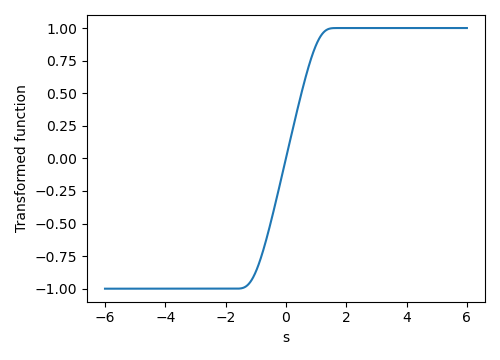
Figure 7: Smooth transformation of piecewise constant function: $f_{1}(s)=-I\{s\leq-2\}$ and $f_{2}(s)=I\{s\geq 2\}$.

The four settings of transition dynamics are specified as the following.

1. Time-homogeneous state transition function and piecewise constant reward function:

   $$S_{0,t+1}=0.5A_{0,t}S_{0,t}+z_{0,t},t\in[0,T].$$

   $$R_{0,t}=\begin{cases}r_{1}(S_{0,t},A_{0,t};t)\equiv-1.5A_{0,t}S_{0,t},&\text{if $t\in[0,T^{*})$}\\ r_{2}(S_{0,t},A_{0,t};t)\equiv A_{0,t}S_{0,t},&\text{if $t\in[T^{*},T]$},\end{cases}$$

2. Time-homogeneous state transition function and smooth reward function:

   $$S_{0,t+1}=0.5A_{0,t}S_{0,t}+z_{0,t},t\in[0,T].$$

   $$R_{0,t}=\begin{cases}r_{1}(S_{0,t},A_{0,t};t),&\text{if $t\in[0,T^{*}-\delta T)$,}\\ g\left(S_{0,t};r_{1},r_{2},T^{*}-\delta T,T^{*}\right),&\text{if $t\in[T^{*}-\delta T,T^{*})$,}\\ r_{2}(S_{0,t},A_{0,t};t),&\text{if $t\in[T^{*},T]$.}\\ \end{cases}$$

3. Piecewise constant state transition and time-homogeneous reward function:

   $$S_{0,t+1}=\begin{cases}F_{1}(S_{0,t},A_{0,t};t)\equiv-0.5A_{0,t}S_{0,t}+z_{0,t},&\text{if $t\in[0,T^{*})$,}\\ F_{2}(S_{0,t},A_{0,t};t)\equiv 0.5A_{0,t}S_{0,t}+z_{0,t},&\text{if $t\in[T^{*},T]$.}\end{cases}$$

   $$R_{0,t}=0.25A_{0,t}S_{0,t}^{2}+4S_{0,t},t\in[0,T].$$

4. Smooth state transition and time-homogeneous reward function:

   $$S_{0,t+1}=\begin{cases}F_{1}(S_{0,t},A_{0,t};t),&\text{if $t\in[0,T^{*})$,}\\ g\left(S_{0,t};F_{1},F_{2},T^{*}-\delta T,T^{*}\right),&\text{if $t\in[T^{*}-\delta T,T^{*})$,}\\ F_{2}(S_{0,t},A_{0,t};t),&\text{if $t\in[T^{*},T]$.}\end{cases}$$

   $$R_{0,t}=0.25A_{0,t}S_{0,t}^{2}+4S_{0,t},t\in[0,T].$$

C.2 Additional Simulation Results

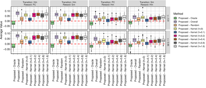
(a) Moderate signal.

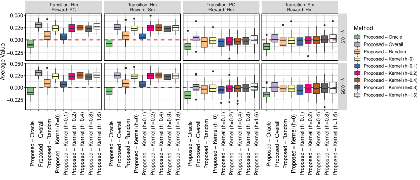
(a) Weak signal.

Figure 9: Distribution of the difference between the expected return under the proposed policy and those under policies computed by other baseline methods, under settings in Section 6.2 with moderate and weak signal-to-noise ratios. The proposed policy is based on the change point detected by the integral type test statistic. In all scenarios, we find the value results based on the normalized or unnormalized test statistics are similar to those of the integral test statistic.

C.3 Simulation Setting of IHS Data

We initiate the state variables as independent normal distributions with $S_{i,0,1}\sim\mathcal{N}(20,3)$, $S_{i,0,2}\sim\mathcal{N}(20,2)$, and $S_{i,0,3}\sim\mathcal{N}(7,1)$, and let them evolve according to

$$\begin{pmatrix}S_{i,t+1,1}\\ S_{i,t+1,2}\\ S_{i,t+1,3}\end{pmatrix}=\bm{W}_{1}(A_{i,t})\tilde{S}_{i,t}I\{t\in[0,T^{*})\}+\bm{W}_{2}(A_{i,t})\tilde{S}_{i,t}I\{t\in[T^{*},T]\}+\bm{z}_{i,t},$$

where the transition matrices are

$$\bm{W}_{1}(A_{i,t}) =\begin{pmatrix}10+0.6A_{i,t}&0.4+0.3A_{i,t}&0.1-0.1A_{i,t}&-0.04&0.1\\ 11-0.4A_{i,t}&0.05&0&0.4&0\\ 1.2-0.5A_{i,t}&-0.02&0&0.03+0.03A_{i,t}&0.8\end{pmatrix},$$

$$\bm{W}_{2}(A_{i,t}) =\begin{pmatrix}10-0.6A_{i,t}&0.4-0.3A_{i,t}&0.1+0.1A_{i,t}&0.04&-0.1\\ 11-0.4A_{i,t}&0.05&0&0.4&0\\ 1.2+0.5A_{i,t}&-0.02&0&0.03-0.03A_{i,t}&0.8\end{pmatrix},$$

$\tilde{S}_{i,t}=(1,S_{i,t})^{\top}$, and $\bm{z}_{i,t}\sim\mathcal{N}_{3}(0,\mathrm{diag}(1,1,0.2))$ is random noise.

References

- Alquier et al., (2019) Alquier, P., Doukhan, P., and Fan, X. (2019). Exponential inequalities for nonstationary Markov chains. Dependence Modeling, 7(1):150–168.
- Aminikhanghahi and Cook, (2017) Aminikhanghahi, S. and Cook, D. (2017). A survey of methods for time series change point detection. Knowledge and Information Systems, 51:339–367.
- Anderson et al., (2020) Anderson, R. M., Heesterbeek, H., Klinkenberg, D., and Hollingsworth, T. D. (2020). How will country-based mitigation measures influence the course of the COVID-19 epidemic? The Lancet, 395(10228):931–934.
- Belloni et al., (2015) Belloni, A., Chernozhukov, V., Chetverikov, D., and Kato, K. (2015). Some new asymptotic theory for least squares series: Pointwise and uniform results. Journal of Econometrics, 186(2):345–366.
- Belloni and Oliveira, (2018) Belloni, A. and Oliveira, R. I. (2018). A high dimensional central limit theorem for martingales, with applications to context tree models. arXiv preprint arXiv:1809.02741.
- Birnbaum, (1942) Birnbaum, Z. W. (1942). An inequality for mill’s ratio. The Annals of Mathematical Statistics, 13(2):245–246.
- Burman and Chen, (1989) Burman, P. and Chen, K.-W. (1989). Nonparametric estimation of a regression function. The Annals of Statististics, 17(4):1567–1596.
- Cazelles et al., (2018) Cazelles, B., Champagne, C., and Dureau, J. (2018). Accounting for non-stationarity in epidemiology by embedding time-varying parameters in stochastic models. PLoS Computational Biology, 14(8):e1006211.
- Chakraborty et al., (2013) Chakraborty, B., Laber, E. B., and Zhao, Y. (2013). Inference for optimal dynamic treatment regimes using an adaptive m-out-of-n bootstrap scheme. Biometrics, 69(3):714–723.
- Chakraborty et al., (2010) Chakraborty, B., Murphy, S., and Strecher, V. (2010). Inference for non-regular parameters in optimal dynamic treatment regimes. Statistical Methods in Medical Research, 19(3):317–343.
- Chen et al., (2022) Chen, E. Y., Song, R., and Jordan, M. I. (2022). Reinforcement learning with heterogeneous data: Estimation and inference. arXiv preprint arXiv:2202.00088.
- Chen and Jiang, (2019) Chen, J. and Jiang, N. (2019). Information-theoretic considerations in batch reinforcement learning. In International Conference on Machine Learning, pages 1042–1051. PMLR.
- Chen, (2007) Chen, X. (2007). Large sample sieve estimation of semi-nonparametric models. Handbook of Econometrics, 6:5549–5632.
- Chen and Christensen, (2015) Chen, X. and Christensen, T. M. (2015). Optimal uniform convergence rates and asymptotic normality for series estimators under weak dependence and weak conditions. Journal of Econometrics, 188(2):447–465.
- Chen and Christensen, (2018) Chen, X. and Christensen, T. M. (2018). Optimal sup-norm rates and uniform inference on nonlinear functionals of nonparametric IV regression. Quantitative Economics, 9(1):39–84.
- Chen et al., (2020) Chen, X., Wang, Y., and Zhou, Y. (2020). Dynamic assortment optimization with changing contextual information. Journal of machine learning research, 21:1–44.
- Chernozhukov et al., (2014) Chernozhukov, V., Chetverikov, D., and Kato, K. (2014). Gaussian approximation of suprema of empirical processes. Ann. Statist., 42(4):1564–1597.
- Cheung et al., (2020) Cheung, W. C., Simchi-Levi, D., and Zhu, R. (2020). Reinforcement learning for non-stationary markov decision processes: The blessing of (more) optimism. In International Conference on Machine Learning, pages 1843–1854. PMLR.
- Cho and Fryzlewicz, (2012) Cho, H. and Fryzlewicz, P. (2012). Multiscale and multilevel technique for consistent segmentation of nonstationary time series. Statistica Sinica, pages 207–229.
- Cho and Fryzlewicz, (2015) Cho, H. and Fryzlewicz, P. (2015). Multiple change-point detection for high-dimensional time series via Sparsified Binary Segmentation. Journal of the Royal Statistical Society: Series B, 77:475–507.
- Csörgö et al., (1997) Csörgö, M., Csörgö, M., and Horváth, L. (1997). Limit theorems in change-point analysis. John Wiley & Sons.
- Dedecker and Fan, (2015) Dedecker, J. and Fan, X. (2015). Deviation inequalities for separately Lipschitz functionals of iterated random functions. Stochastic Processes and their Applications, 125(1):60–90.
- DeVore and Lorentz, (1993) DeVore, R. A. and Lorentz, G. G. (1993). Constructive approximation, volume 303. Springer Science & Business Media.
- Domingues et al., (2021) Domingues, O. D., Ménard, P., Pirotta, M., Kaufmann, E., and Valko, M. (2021). A kernel-based approach to non-stationary reinforcement learning in metric spaces. In International Conference on Artificial Intelligence and Statistics, pages 3538–3546. PMLR.
- Eftekhari et al., (2020) Eftekhari, H., Mukherjee, D., Banerjee, M., and Ritov, Y. (2020). Markovian and non-Markovian processes with active decision making strategies for addressing the COVID-19 pandemic. arXiv preprint arXiv:2008.00375.
- Eichenbaum et al., (2020) Eichenbaum, M. S., Rebelo, S., and Trabandt, M. (2020). The macroeconomics of epidemics. Technical report, National Bureau of Economic Research.
- Ernst et al., (2005) Ernst, D., Geurts, P., and Wehenkel, L. (2005). Tree-based batch mode reinforcement learning. Journal of Machine Learning Research, 6:503–556.
- Ertefaie and Strawderman, (2018) Ertefaie, A. and Strawderman, R. L. (2018). Constructing dynamic treatment regimes over indefinite time horizons. Biometrika, 105(4):963–977.
- Fan et al., (2020) Fan, J., Wang, Z., Xie, Y., and Yang, Z. (2020). A theoretical analysis of deep q-learning. In Learning for Dynamics and Control, pages 486–489. PMLR.
- Fang et al., (2022) Fang, E. X., Wang, Z., and Wang, L. (2022). Fairness-oriented learning for optimal individualized treatment rules. Journal of the American Statistical Association, just-accepted:1–14.
- Fei et al., (2020) Fei, Y., Yang, Z., Wang, Z., and Xie, Q. (2020). Dynamic regret of policy optimization in non-stationary environments. In Advances in Neural Information Processing Systems, pages 6743–6754.
- Fryzlewicz, (2014) Fryzlewicz, P. (2014). Wild Binary Segmentation for multiple change-point detection. The Annals of Statistics, 42:2243–2281.
- Garreau et al., (2017) Garreau, D., Jitkrittum, W., and Kanagawa, M. (2017). Large sample analysis of the median heuristic. arXiv preprint arXiv:1707.07269.
- Hao et al., (2021) Hao, B., Ji, X., Duan, Y., Lu, H., Szepesvari, C., and Wang, M. (2021). Bootstrapping fitted q-evaluation for off-policy inference. In International Conference on Machine Learning, pages 4074–4084. PMLR.
- Hasselt, (2010) Hasselt, H. V. (2010). Double Q-learning. In Advances in Neural Information Processing Systems, pages 2613–2621.
- (36) Hu, X., Qian, M., Cheng, B., and Cheung, Y. K. (2021a). Personalized policy learning using longitudinal mobile health data. Journal of the American Statistical Association, 116(533):410–420.
- (37) Hu, Y., Kallus, N., and Uehara, M. (2021b). Fast rates for the regret of offline reinforcement learning. arXiv preprint arXiv:2102.00479.
- Huang, (1998) Huang, J. Z. (1998). Projection estimation in multiple regression with application to functional ANOVA models. The Annals of Statistics, 26(1):242–272.
- Judd, (1998) Judd, K. L. (1998). Numerical methods in economics. MIT press.
- Killick et al., (2012) Killick, R., Fearnhead, P., and Eckley, I. (2012). Optimal detection of changepoints with a linear computational cost. Journal of the American Statistical Association, 107(500):1590–1598.
- Klasnja et al., (2019) Klasnja, P., Smith, S., Seewald, N. J., Lee, A., Hall, K., Luers, B., Hekler, E. B., and Murphy, S. A. (2019). Efficacy of contextually tailored suggestions for physical activity: A micro-randomized optimization trial of Heartsteps. Annals of Behavioral Medicine, 53(6):573–582.
- Kompella et al., (2020) Kompella, V., Capobianco, R., Jong, S., Browne, J., Fox, S., Meyers, L., Wurman, P., and Stone, P. (2020). Reinforcement learning for optimization of COVID-19 mitigation policies. arXiv preprint arXiv:2010.10560.
- Kosorok and Laber, (2019) Kosorok, M. R. and Laber, E. B. (2019). Precision medicine. Annual review of statistics and its application, 6:263–286.
- Le et al., (2019) Le, H., Voloshin, C., and Yue, Y. (2019). Batch policy learning under constraints. In International Conference on Machine Learning, pages 3703–3712.
- Lecarpentier and Rachelson, (2019) Lecarpentier, E. and Rachelson, E. (2019). Non-stationary markov decision processes, a worst-case approach using model-based reinforcement learning. Advances in Neural Information Processing Systems, 32.
- Li, (2019) Li, Y. (2019). Reinforcement learning applications. arXiv preprint arXiv:1908.06973.
- (47) Liao, P., Greenewald, K., Klasnja, P., and Murphy, S. (2020a). Personalized Heartsteps: A reinforcement learning algorithm for optimizing physical activity. Proceedings of the ACM on Interactive, Mobile, Wearable and Ubiquitous Technologies, 4(1):1–22.
- Liao et al., (2021) Liao, P., Klasnja, P., and Murphy, S. (2021). Off-policy estimation of long-term average outcomes with applications to mobile health. Journal of the American Statistical Association, 116(533):382–391.
- (49) Liao, P., Qi, Z., and Murphy, S. (2020b). Batch policy learning in average reward Markov decision processes. arXiv preprint arXiv:2007.11771.
- Luckett et al., (2020) Luckett, D. J., Laber, E. B., Kahkoska, A. R., Maahs, D. M., Mayer-Davis, E., and Kosorok, M. R. (2020). Estimating dynamic treatment regimes in mobile health using V-learning. Journal of the American Statistical Association, 115(530):692–706.
- Luedtke and van der Laan, (2016) Luedtke, A. R. and van der Laan, M. J. (2016). Statistical inference for the mean outcome under a possibly non-unique optimal treatment strategy. The Annals of Statistics, 44(2):713–742.
- Maei et al., (2010) Maei, H. R., Szepesvári, C., Bhatnagar, S., and Sutton, R. S. (2010). Toward off-policy learning control with function approximation. In ICML, pages 719–726.
- Marling and Bunescu, (2020) Marling, C. and Bunescu, R. (2020). The OhioT1DM dataset for blood glucose level prediction: Update 2020. In CEUR Workshop Proceedings, volume 2675, page 71.
- McLeish, (1974) McLeish, D. L. (1974). Dependent central limit theorems and invariance principles. Ann. Probability, 2:620–628.
- Meinshausen et al., (2009) Meinshausen, N., Meier, L., and Bühlmann, P. (2009). P-values for high-dimensional regression. Journal of the American Statistical Association, 104(488):1671–1681.
- Mendelson et al., (2008) Mendelson, S., Pajor, A., and Tomczak-Jaegermann, N. (2008). Uniform uncertainty principle for bernoulli and subgaussian ensembles. Constructive Approximation, 28(3):277–289.
- Mnih et al., (2015) Mnih, V., Kavukcuoglu, K., Silver, D., Rusu, A. A., Veness, J., Bellemare, M. G., Graves, A., Riedmiller, M., Fidjeland, A. K., Ostrovski, G., et al. (2015). Human-level control through deep reinforcement learning. Nature, 518(7540):529–533.
- Munos and Szepesvári, (2008) Munos, R. and Szepesvári, C. (2008). Finite-time bounds for fitted value iteration. Journal of Machine Learning Research, 9(5).
- Murphy, (2003) Murphy, S. A. (2003). Optimal dynamic treatment regimes. Journal of the Royal Statistical Society. Series B. Statistical Methodology, 65(2):331–366.
- NeCamp et al., (2020) NeCamp, T., Sen, S., Frank, E., Walton, M. A., Ionides, E. L., Fang, Y., Tewari, A., and Wu, Z. (2020). Assessing real-time moderation for developing adaptive mobile health interventions for medical interns: Micro-randomized trial. Journal of Medical Internet Research, 22(3):e15033.
- Nie et al., (2021) Nie, X., Brunskill, E., and Wager, S. (2021). Learning when-to-treat policies. Journal of the American Statistical Association, 116(533):392–409.
- Niroui et al., (2019) Niroui, F., Zhang, K., Kashino, Z., and Nejat, G. (2019). Deep reinforcement learning robot for search and rescue applications: Exploration in unknown cluttered environments. IEEE Robotics and Automation Letters, 4(2):610–617.
- Padakandla et al., (2020) Padakandla, S., Prabuchandran, K., and Bhatnagar, S. (2020). Reinforcement learning algorithm for non-stationary environments. Applied Intelligence, 50(11):3590–3606.
- Puterman, (1994) Puterman, M. L. (1994). Markov decision processes: discrete stochastic dynamic programming. Wiley Series in Probability and Mathematical Statistics: Applied Probability and Statistics. John Wiley & Sons, Inc., New York. A Wiley-Interscience Publication.
- Qi et al., (2020) Qi, Z., Liu, D., Fu, H., and Liu, Y. (2020). Multi-armed angle-based direct learning for estimating optimal individualized treatment rules with various outcomes. Journal of the American Statistical Association, 115(530):678–691.
- Qian and Murphy, (2011) Qian, M. and Murphy, S. A. (2011). Performance guarantees for individualized treatment rules. The Annals of Statistics, 39(2):1180–1210.
- Qian et al., (2022) Qian, T., Walton, A. E., Collins, L. M., Klasnja, P., Lanza, S. T., Nahum-Shani, I., Rabbi, M., Russell, M. A., Walton, M. A., Yoo, H., et al. (2022). The microrandomized trial for developing digital interventions: Experimental design and data analysis considerations. Psychological Methods.
- Rahimi and Recht, (2007) Rahimi, A. and Recht, B. (2007). Random features for large-scale kernel machines. In Platt, J., Koller, D., Singer, Y., and Roweis, S., editors, Advances in Neural Information Processing Systems, volume 20. Curran Associates, Inc.
- Ramprasad et al., (2021) Ramprasad, P., Li, Y., Yang, Z., Wang, Z., Sun, W. W., and Cheng, G. (2021). Online bootstrap inference for policy evaluation in reinforcement learning. arXiv preprint arXiv:2108.03706.
- Robins, (2004) Robins, J. M. (2004). Optimal structural nested models for optimal sequential decisions. In Proceedings of the Second Seattle Symposium in Biostatistics, pages 189–326. Springer.
- (71) Shi, C., Lu, W., and Song, R. (2020a). Breaking the curse of nonregularity with subagging—inference of the mean outcome under optimal treatment regimes. Journal of Machine Learning Research, 21(176):1–67.
- Shi et al., (2018) Shi, C., Song, R., Lu, W., and Fu, B. (2018). Maximin projection learning for optimal treatment decision with heterogeneous individualized treatment effects. Journal of Royal Statistical Society: Series B, 80(4):681–702.
- (73) Shi, C., Wan, R., Song, R., Lu, W., and Leng, L. (2020b). Does the Markov decision process fit the data: Testing for the Markov property in sequential decision making. In International Conference on Machine Learning, pages 8807–8817. PMLR.
- Shi et al., (2021) Shi, C., Zhang, S., Lu, W., and Song, R. (2021). Statistical inference of the value function for reinforcement learning in infinite horizon settings. Journal of Royal Statistical Society: Series B, accepted.
- Song et al., (2015) Song, R., Wang, W., Zeng, D., and Kosorok, M. R. (2015). Penalized Q-learning for dynamic treatment regimens. Statistica Sinica, 25(3):901–920.
- Sutton and Barto, (2018) Sutton, R. S. and Barto, A. G. (2018). Reinforcement Learning: An Introduction. Adaptive Computation and Machine Learning. MIT Press, Cambridge, MA, second edition.
- Tropp, (2011) Tropp, J. (2011). Freedman’s inequality for matrix martingales. Electronic Communications in Probability, 16:262–270.
- Truong et al., (2020) Truong, C., Oudre, L., and Vayatis, N. (2020). Selective review of offline change point detection methods. Signal Processing, 167. 107299.
- Tsiatis et al., (2019) Tsiatis, A. A., Davidian, M., Holloway, S. T., and Laber, E. B. (2019). Dynamic Treatment Regimes: Statistical Methods for Precision Medicine. CRC press.
- Uehara et al., (2021) Uehara, M., Imaizumi, M., Jiang, N., Kallus, N., Sun, W., and Xie, T. (2021). Finite sample analysis of minimax offline reinforcement learning: Completeness, fast rates and first-order efficiency. arXiv preprint arXiv:2102.02981.
- van der Vaart and Wellner, (1996) van der Vaart, A. W. and Wellner, J. A. (1996). Weak convergence and empirical processes. Springer Series in Statistics. Springer-Verlag, New York.
- Wallace and Moodie, (2015) Wallace, M. P. and Moodie, E. E. M. (2015). Doubly-robust dynamic treatment regimen estimation via weighted least squares. Biometrics, 71(3):636–644.
- Wan et al., (2020) Wan, R., Zhang, X., and Song, R. (2020). Multi-objective reinforcement learning for infectious disease control with application to covid-19 spread. arXiv preprint arXiv:2009.04607.
- Wang et al., (2018) Wang, L., Zhou, Y., Song, R., and Sherwood, B. (2018). Quantile-optimal treatment regimes. J. Amer. Stat. Assoc., 113(523):1243–1254.
- Wang and Samworth, (2018) Wang, T. and Samworth, R. (2018). High dimensional change point estimation via sparse projection. Journal of the Royal Statistical Society: Series B, 80:57–83.
- Watkins and Dayan, (1992) Watkins, C. J. and Dayan, P. (1992). Q-learning. Machine learning, 8(3-4):279–292.
- Wei and Luo, (2021) Wei, C.-Y. and Luo, H. (2021). Non-stationary reinforcement learning without prior knowledge: An optimal black-box approach. In Conference on Learning Theory, pages 4300–4354. PMLR.
- Xie et al., (2021) Xie, A., Harrison, J., and Finn, C. (2021). Deep reinforcement learning amidst continual structured non-stationarity. In International Conference on Machine Learning, pages 11393–11403. PMLR.
- Yu and Chen, (2021) Yu, M. and Chen, X. (2021). Finite sample change point inference and identification for high-dimensional mean vectors. Journal of the Royal Statistical Society: Series B, 83(2):247–270.
- Zhang et al., (2013) Zhang, B., Tsiatis, A. A., Laber, E. B., and Davidian, M. (2013). Robust estimation of optimal dynamic treatment regimes for sequential treatment decisions. Biometrika, 100(3):681–694.
- Zhang et al., (2018) Zhang, Y., Laber, E. B., Davidian, M., and Tsiatis, A. A. (2018). Estimation of optimal treatment regimes using lists. Journal of American Statistical Association, 113(524):1541–1549.
- Zhao et al., (2015) Zhao, Y.-Q., Zeng, D., Laber, E. B., and Kosorok, M. R. (2015). New statistical learning methods for estimating optimal dynamic treatment regimes. Journal of American Statistical Association, 110(510):583–598.
- Zhong et al., (2021) Zhong, H., Yang, Z., and Szepesvári, Z. W. C. (2021). Optimistic policy optimization is provably efficient in non-stationary MDPs. arXiv preprint arXiv:2110.08984.
- Zhu et al., (2017) Zhu, R., Zhao, Y.-Q., Chen, G., Ma, S., and Zhao, H. (2017). Greedy outcome weighted tree learning of optimal personalized treatment rules. Biometrics, 73(2):391–400.