Capturing Shape Information with Multi-Scale Topological Loss Terms for 3D Reconstruction

Abstract

Reconstructing 3D objects from 2D images is both challenging for our brains and machine learning algorithms. To support this spatial reasoning task, contextual information about the overall shape of an object is critical. However, such information is not captured by established loss terms (e.g. Dice loss). We propose to complement geometrical shape information by including multi-scale topological features, such as connected components, cycles, and voids, in the reconstruction loss. Our method uses cubical complexes to calculate topological features of 3D volume data and employs an optimal transport distance to guide the reconstruction process. This topology-aware loss is fully differentiable, computationally efficient, and can be added to any neural network. We demonstrate the utility of our loss by incorporating it into SHAPR, a model for predicting the 3D cell shape of individual cells based on 2D microscopy images. Using a hybrid loss that leverages both geometrical and topological information of single objects to assess their shape, we find that topological information substantially improves the quality of reconstructions, thus highlighting its ability to extract more relevant features from image datasets.

1 Introduction

Segmentation and reconstruction are common tasks when dealing with imaging data. Especially in the biomedical domain, segmentation accuracy can have a substantial impact on complex downstream tasks, such as a patient’s diagnosis and treatment. 3D segmentation is a complex task in itself, requiring the assessment and labelling of each voxel in a volume, which, in turn, necessitates a high-level understanding of the object and its context. However, complexity rapidly increases when attempting to reconstruct a 3D object from a 2D projection since 3D images may often be difficult to obtain. This constitutes an inverse problem with intrinsically ambiguous solutions: each 2D image permits numerous 3D reconstructions, similar to how a shadow alone does not necessarily permit conclusions to be drawn about the corresponding shape. When addressed using machine learning, the solution of such inverse problems can be facilitated by imbuing a model with additional inductive biases about the structural properties of objects. Existing models supply such inductive biases to the reconstruction task mainly via geometry-based objective functions, thus learning a likelihood function $f\colon\mathcal{V}\to\mathds{R}$, where $f(x)$ for $x\in\mathcal{V}$ denotes the likelihood that a voxel $x$ of the input volume $\mathcal{V}$ is part of the ground truth shape [18]. Loss functions to learn $f$ are evaluated on a per-voxel basis, assessing the differences between the original volume and the predicted volume in terms of overlapping labels. Commonly-used loss functions include binary cross entropy (BCE), Dice loss, and mean squared error (MSE). Despite their expressive power, these loss terms do not capture structural shape properties of the volumes.

Our contributions.

Topological features, i.e. features that characterise data primarily in terms of connectivity, have recently started to emerge as a powerful paradigm for complementing existing machine learning methods [13]. They are capable of capturing shape information of objects at multiple scales and along multiple dimensions. In this paper, we leverage such features and integrate them into a novel differentiable ‘topology-aware’ loss term $\operatorname{\mathcal{L}}_{\text{T}}$ that can be used to regularise the shape reconstruction process. Our loss term handles arbitrary shapes, can be computed efficiently, and may be integrated into general deep learning models. We demonstrate the utility of $\operatorname{\mathcal{L}}_{\text{T}}$ by combining it with SHAPR [29], a framework for predicting individual cell shapes from 2D microscopy images. The new hybrid variant of SHAPR, making use of both geometry-based and topology-based objective functions, results in improved reconstruction performance along multiple metrics.

2 Related Work

Several deep learning approaches for predicting 3D shapes of single objects from 2D information already exist; we aim to give a brief overview. Previous work includes predicting natural objects such as air planes, cars, and furniture from photographs, creating either meshes [11, 30], voxel volumes [3], or point clouds [9]. A challenging biomedical task, due to the occurrence of imaging noise, is tackled by Waibel et al. [29], whose SHAPR model predicts the shape and morphology of individual mammalian cells from 2D microscopy images. Given the multi-scale nature of microscopy images, SHAPR is an ideal use case to analyse the impact of employing additional topology-based loss terms for these reconstruction tasks.

Such loss terms constitute a facet of the emerging field of topological machine learning and persistent homology, its flagship algorithm (see Section 3.1 for an introduction). Previous studies have shown great promise in using topological losses for image segmentation tasks or their evaluation [25]. In contrast to our loss, existing work relies on prior knowledge about ‘expected’ topological features [4], or enforces a pre-defined set of topological features based on comparing segmentations [15, 16].

3 Our Method: A Topology-Aware Loss

We propose a topology-aware loss term based on concepts from topological machine learning and optimal transport. The loss term works on the level of individual volumes, leveraging a valid metric between topological descriptors, while remaining efficiently computable. Owing to its generic nature, the loss can be easily integrated into existing architectures; see Fig. 1 for an overview.

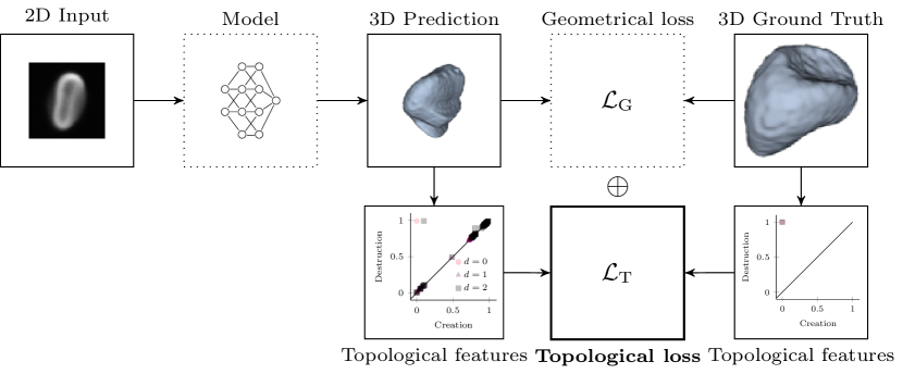
Figure 1: Given a predicted object and a 3D ground truth object, we calculate topological features using cubical persistent homology, obtaining a set of persistence diagrams. Each point in a persistence diagram denotes the creation and destruction of a $d$-dimensional topological feature of the given object. We compare these diagrams using $\operatorname{\mathcal{L}}_{\text{T}}$, our novel topology-based loss, combining it with geometrical loss terms such as binary cross entropy (BCE). Dotted components can be swapped out.

3.1 Assessing the Topology of Volumes

Given a volume $\mathcal{V}$, i.e. a $d$-dimensional tensor of shape $n_{1}\times n_{2}\times\dots\times n_{d}$, we represent it as a cubical complex $C$. A cubical complex contains individual voxels of $\mathcal{V}$ as vertices , along with connectivity information about their neighbourhoods via edges , squares , and their higher-dimensional counterparts. Cubical complexes provide a fundamental way to represent volume data and have proven their utility in previous work [24, 28]. Topological features of different dimensions are well-studied, comprising connected components (0D), cycles (1D), and voids (2D), for instance. The number of $k$-dimensional topological features is also referred to as the $k$th Betti number $\beta_{k}$ of $C$. While previous work has shown the efficacy of employing Betti numbers as a topological prior for image segmentation tasks [4, 15], the reconstruction tasks we are considering in this paper require a multi-scale perspective that cannot be provided by Betti numbers, which are mere feature counts. We therefore make use of persistent homology, a technique for calculating multi-scale topological features [8]. This technique is particularly appropriate in our setting: our model essentially learns a likelihood function $f\colon\mathcal{V}\to\mathds{R}$. To each voxel $x\in\mathcal{V}$, the function $f$ assigns the likelihood of $x$ being part of an object’s shape. For a likelihood threshold $\tau\in\mathds{R}$, we obtain a cubical complex $C^{(\tau)}:=\{x\in\mathcal{V}\mid f(x)\geq\tau\}$ and, consequently, a different set of topological features. Since volumes are finite, their topology only changes at a finite number of thresholds $\tau_{1}\geq\dotsc\geq\tau_{m}$, and we obtain a sequence of nested cubical complexes $\emptyset\subseteq C^{(\tau_{1})}\subseteq C^{(\tau_{2})}\subseteq\dots\subseteq C^{(\tau_{m})}=\mathcal{V}$, known as a superlevel set filtration. Persistent homology tracks topological features across all complexes in this filtration, representing each feature as a tuple $(\tau_{i},\tau_{j})$, with $\tau_{i}\geq\tau_{j}$, indicating the cubical complex in which a feature was being ‘created’ and ‘destroyed,’ respectively. The tuples of $k$-dimensional features, with $0\leq k\leq d$, are stored in the $k$th persistence diagram $\mathcal{D}_{f}^{(k)}$ of the data set. Persistence diagrams thus form a multi-scale shape descriptor of all topological features of a dataset. Despite the apparent complexity of filtrations, persistent homology of cubical complexes can be calculated efficiently in practice [28].

Structure of persistence diagrams.

Persistent homology provides information beyond Betti numbers: instead of enforcing a choice of threshold $\tau$ for the likelihood function, which would result in a fixed set of Betti numbers, persistence diagrams encode all thresholds at the same time, thus capturing additional geometrical details about data. Given a tuple $(\tau_{i},\tau_{j})$ in a persistence diagram, its persistence is defined as $\operatorname{pers}\left(\tau_{i},\tau_{j}\right):=\left|\tau_{j}-\tau_{i}\right|$. Persistence indicates the ‘scale’ over which a topological feature occurs, with large values typically assumed to correspond to more stable features. The sum of all persistence values is known as the degree-$p$ total persistence, i.e. $\operatorname{Pers}_{p}(\mathcal{D}_{f}):=\sum_{(\tau_{i},\tau_{j})\in\mathcal{D}_{f}}\left|\operatorname{pers}(\tau_{i},\tau_{j})^{p}\right|$. It constitutes a stable summary statistic of topological activity [7].

Comparing persistence diagrams.

Persistence diagrams can be endowed with a metric by using optimal transport. Given two diagrams $\mathcal{D}$ and $\mathcal{D}^{\prime}$ containing features of the same dimensionality, their $p$th Wasserstein distance is defined as

$$\operatorname{W}_{p}\left(\mathcal{D},\mathcal{D}^{\prime}\right):=\left(\inf_{\eta\colon\mathcal{D}\to\mathcal{D}^{\prime}}\sum_{x\in\mathcal{D}}\|x-\eta(x)\|_{\infty}^{p}\right)^{\frac{1}{p}},$$ (1)

where $\eta(\cdot)$ denotes a bijection. Since $\mathcal{D}$ and $\mathcal{D}^{\prime}$ generally have different cardinalities, we consider them to contain an infinite number of points of the form $(\tau,\tau)$, i.e. tuples of zero persistence. A suitable $\eta(\cdot)$ can thus always be found. Solving Eq. 1 is practically feasible using modern optimal transport algorithms [10].

Stability.

A core property of persistence diagrams is their stability to noise. While different notions of stability exist for persistent homology [7], a recent theorem [27] states that the Wasserstein distance between persistence diagrams of functions $f,f^{\prime}\colon\mathcal{V}\to\mathds{R}$ is bounded by their $p$-norm, i.e.

$$\operatorname{W}_{p}\left(\mathcal{D}_{f}^{(k)},\mathcal{D}_{f^{\prime}}^{(k)}\right)\leq C\left\|f-f^{\prime}\right\|_{p}\text{ for $0\leq k\leq d$},$$ (2)

with $C\in\mathds{R}_{>0}$ being a constant that depends on the dimensionality of $\mathcal{V}$. Eq. 2 implies that gradients obtained from the Wasserstein distance and other topology-based summaries will remain bounded; we will also use it to accelerate topological feature calculations in practice.

Differentiability.

Despite the discrete nature of topological features, persistent homology permits the calculation of gradients with respect to parameters of the likelihood function $f$, thus enabling the use of automatic differentiation schemes [14, 19, 22]. A seminal work by Carrière et al. [2] proved that optimisation algorithms converge for a wide class of persistence-based functions, thus opening the door towards general topology-based optimisation schemes.

3.2 Loss Term Construction

Given a true likelihood function $f$ and a predicted likelihood function $f^{\prime}$, our novel generic topology-aware loss term takes the form

$$\operatorname{\mathcal{L}}_{\text{T}}\left(f,f^{\prime},p\right):=\sum_{i=0}^{d}\operatorname{W}_{p}\left(\mathcal{D}_{f}^{(i)},\mathcal{D}_{f^{\prime}}^{(i)}\right)+\operatorname{Pers}\left(\mathcal{D}_{f^{\prime}}^{(i)}\right).$$ (3)

The first part of Eq. 3 incentivises the model to reduce the distance between $f$ and $f^{\prime}$ with respect to their topological shape information. The second part incentivises the model to reduce overall topological activity, thus decreasing the noise in the reconstruction. This can be considered as the topological equivalent of reducing the total variation of a function [23]. Given a task-specific geometrical loss term $\operatorname{\mathcal{L}}_{\text{G}}$, such as a Dice loss, we obtain a combined loss term as $\operatorname{\mathcal{L}}:=\operatorname{\mathcal{L}}_{\text{G}}+\lambda\operatorname{\mathcal{L}}_{\text{T}}$, where $\lambda\in\mathds{R}_{>0}$ controls the impact of the topology-based part. We will use $p=2$ since Eq. 2 relates $\operatorname{\mathcal{L}}_{\text{T}}$ to the Euclidean distance in this case.

Calculations in practice.

To speed up the calculation of our loss term, we utilise the stability theorem of persistent homology and downsample each volume to $M\times M\times M$ voxels using trilinear interpolation. We provide a theoretical and empirical analysis of the errors introduced by downsampling in the Supplementary Materials. In our experiments, we set $M=16$, which is sufficiently small to have no negative impact on computational performance while at the same time resulting in empirical errors $\leq 0.1$ (measured using Eq. 2 for $p=2$).

4 Experiments

We provide a brief overview of SHAPR before discussing the experimental setup, datasets, and results. SHAPR is a deep learning method to predict 3D shapes of single cells from 2D microscopy images [29]. Given a 2D fluorescent image of a single cell and a corresponding segmentation mask, SHAPR predicts the 3D shape of this cell. The authors suggest to train SHAPR with a combination of Dice and BCE loss, with an additional adversarial training step to improve the predictions of the model. We re-implemented SHAPR using PyTorch [21] to ensure fair comparisons and the seamless integration of our novel loss function $\operatorname{\mathcal{L}}_{\text{T}}$, employing ‘Weights & Biases’ for tracking experiments [1]. Our code and reports are publicly available.

Data.

For our experiments, we use the two datasets published with the original SHAPR manuscript [29]. The first dataset comprises $825$ red blood cells, imaged in 3D with a confocal microscope [26]. Each cell is assigned to one of nine pre-defined classes: sphero-, stomato-, disco-, echino-, kerato-, knizo-, and acanthocytes, as well as cell clusters and multilobates. The second dataset contains $887$ nuclei of human-induced pluripotent stem cells (iPSCs), counterstained and imaged in 3D with a confocal microscope. Cells were manually segmented to create ground truth objects. Both datasets include 3D volumes of size $64\times 64\times 64$, 2D segmentation masks of size $64\times 64$, and fluorescent images of size $64\times 64$.

4.1 Training and Evaluation

We trained our implementation of SHAPR for a maximum of $100$ epochs, using early stopping with a patience of $15$ epochs, based on the validation loss. For each run, we trained five SHAPR models in a round-robin fashion, partitioning the dataset into five folds with a 60%/20%/20% train/validation/test split, making sure that each 2D input image appears once in the test set. To compare the performance of SHAPR with and without $\operatorname{\mathcal{L}}_{\text{T}}$, we used the same hyperparameters for all experiments (initial learning rate of $1\text{\times}{10}^{-3}$, $\beta_{1}=0.9$, and $\beta_{2}=0.999$ for the ADAM optimiser). We optimised $\lambda\in\{$1\text{\times}{10}^{-3}$,$1\text{\times}{10}^{-2}$,\dots,$1\text{\times}{10}^{2}$\}$, the regularisation strength parameter for $\operatorname{\mathcal{L}}_{\text{T}}$, on an independent dataset, resulting in $\lambda=0.1$ for all experiments. We also found that evaluating Eq. 3 for each dimension individually leads to superior performance; we thus only calculate Eq. 3 for $i=2$. Finally, for the training phase, we augmented the data with random horizontal or vertical flipping and $90^{\circ}$ rotations with a 33% chance for each augmentation to be applied for a sample. The goal of these augmentations is to increase data variability and prevent overfitting.

Following Waibel et al. [29], we evaluated the performance of SHAPR by calculating (i) the intersection over union (IoU) error, (ii) the relative volume error, (iii) the relative surface area error, and (iv) the relative surface roughness error with respect to the ground truth data, applying Otsu’s method [20] for thresholding predicted shapes. We calculate the volume by counting non-zero voxels, the surface area as all voxels on the surface of an object, and the surface roughness as the difference between the surface area of the object and the surface area of the same object after smoothing it with a 3D Gaussian [29].

(a)

(b)

Figure 2: 2(a) Examples of predictions without (top row) and with (middle row) $\operatorname{\mathcal{L}}_{\text{T}}$, our topological loss term. The third row shows ground truth images. 2(b) $\operatorname{\mathcal{L}}_{\text{T}}$ improves predictions in relevant metrics, such as the IoU error, the relative volume error, relative surface area error, and relative surface roughness error.

4.2 Results

To evaluate the benefits of our topology-aware loss, we perform the same experiment twice: first, using a joint BCE and Dice loss [29], followed by adding $\lambda\operatorname{\mathcal{L}}_{\text{T}}$. Without $\operatorname{\mathcal{L}}_{\text{T}}$, we achieve results comparable to the original publication (IoU, red blood cell data: $0.63\pm 0.12\%$; IoU, nuclei data: $0.46\pm 0.16\%$); minor deviations arise from stochasticity and implementation differences between PyTorch and Tensorflow. We observe superior performance in the majority of metrics for both datasets when adding $\operatorname{\mathcal{L}}_{\text{T}}$ to the model (see Fig. 2 and Table 1); the performance gains by $\operatorname{\mathcal{L}}_{\text{T}}$ are statistically significant in all but one case. Notably, we find that $\operatorname{\mathcal{L}}_{\text{T}}$ increases SHAPR’s predictive performance unevenly across the classes of the red blood cell dataset (see Fig. 2(a)). For spherocytes (round cells), only small changes in IoU error, relative volume error, relative surface area error, and relative surface roughness error (7% decrease, 2% decrease, and 3% decrease, respectively) occur, whereas for echinocytes (cells with a spiky surface), we obtain a 27% decrease in IoU error and 7% decrease in relative volume error. Finally, for discocytes (bi-concave cells) and stomatocytes, we obtain a 2% decrease in IoU error, a 3% decrease in volume error, a 11% decrease in surface area error, and a 25% decrease in surface roughness error upon adding $\operatorname{\mathcal{L}}_{\text{T}}$.

Table 1: Median, mean ($\mu$) and standard deviation ($\sigma$) of several relative error measures for two datasets (lower values are better; winner shown in bold). The $\operatorname{\mathcal{L}}_{\text{T}}$ column indicates whether our new loss term was active. We also show the $p$-value of a paired Wilcoxon signed-rank test between error distributions.

		Red blood cell ($n=825$)			Nuclei ($n=887$)
Relative error	$\operatorname{\mathcal{L}}_{\text{T}}$	Median	$\mu\pm\sigma$	$p$	Median	$\mu\pm\sigma$	$p$
$1-\mathrm{IoU}$	✗	$0.48$	$0.49$ p m 0.09	$1.1\text{\times}{10}^{-19}$	$0.62$	$0.62$ p m 0.11	$0.491$
	✓	$0.47$	$0.47$ p m 0.10		$0.61$	$0.61$ p m 0.11
Volume	✗	$0.31$	$0.35$ p m 0.31	$1.2\text{\times}{10}^{-47}$	$0.34$	$0.48$ p m 0.47	$4.6\text{\times}{10}^{-14}$
	✓	$0.26$	$0.29$ p m 0.27		$0.32$	$0.43$ p m 0.42
Surface area	✗	$0.20$	$0.24$ p m 0.20	$39.5\text{\times}{10}^{-13}$	$0.21$	$0.27$ p m 0.25	$1.7\text{\times}{10}^{-8}$
	✓	$0.14$	$0.18$ p m 0.16		$0.18$	$0.25$ p m 0.24
Surface roughness	✗	$0.35$	$0.36$ p m 0.24	$9.1\text{\times}{10}^{-4}$	$0.17$	$0.18$ p m 0.12	$1.5\text{\times}{10}^{-6}$
	✓	$0.24$	$0.29$ p m 0.22		$0.18$	$0.19$ p m 0.13

5 Discussion

We propose a novel topology-aware loss term $\operatorname{\mathcal{L}}_{\text{T}}$ that can be integrated into existing deep learning models. Our loss term is not restricted to specific types of shapes and may be applied to reconstruction and segmentation tasks. We demonstrate its efficacy in the reconstruction of 3D shapes from 2D microscopy images, where the results of SHAPR are statistically significantly improved in relevant metrics whenever $\operatorname{\mathcal{L}}_{\text{T}}$ is jointly optimised together with geometrical loss terms. Notably, $\operatorname{\mathcal{L}}_{\text{T}}$ does not optimise classical segmentation/reconstruction metrics, serving instead as an inductive bias for incorporating multi-scale information on topological features. $\operatorname{\mathcal{L}}_{\text{T}}$ is computationally efficient and can be adapted to different scenarios by incorporating topological features of a specific dimension. Since our experiments indicate that the calculation of Eq. 3 for a single dimension is sufficient to achieve improved reconstruction results in practice, we will leverage topological duality/symmetry theorems [6] in future work to improve computational efficiency and obtain smaller cubical complexes.

Our analysis of predictive performance across classes of the red blood cell dataset (see Table 1) leads to the assumption that the topological loss term shows the largest reconstruction performance increases on shapes that have complex morphological features, such as echinocytes or bi-concavely shaped cells (discocytes and stomatocytes). This implies that future extensions of the method should incorporate additional geometrical descriptors into the filtration calculation, making use of recent advances in capturing the topology of multivariate shape descriptors [17].

5.0.1 Acknowledgements.

We thank Lorenz Lamm, Melanie Schulz, Kalyan Varma Nadimpalli, and Sophia Wagner for their valuable feedback to this manuscript. The authors also are indebted to Teresa Heiss for discussions on the topological changes induced by downsampling volume data.

5.0.2 Funding.

Carsten Marr received funding from the European Research Council (ERC) under the European Union’s Horizon 2020 Research and Innovation Programme (Grant Agreement 866411).

5.0.3 Author contributions.

DW and BR implemented code and conducted experiments. DW, BR, and CM wrote the manuscript. DW created figures and BR the main portrayal of results. SA and MM provided the 3D nuclei dataset. BR supervised the study. All authors have read and approved the manuscript.

Appendix 0.A Discussion: The Effects of Interpolation

As outlined in the main paper, we downsample our volumes from $64^{3}$ voxels to $16^{3}$ voxels using trilinear interpolation. To assess the impact this has on the calculation of persistent homology, we can make use of recent work on the topological impact of changing image resolutions [12]. Following Heiss et al. [12], we treat downsampling as a general function that transforms a volume of side length $r_{1}\in\mathds{N}$ into a volume of side length $r_{2}\in\mathds{N}$. Assuming that $r_{1}>r_{2}>0$ and $r_{2}\mid r_{1}$, we refer to $a:=\nicefrac{{r_{1}}}{{r_{2}}}$ as the compression factor. In $d$ dimensions, every voxel of size $r_{2}$ contains $a^{d}$ voxels of size $r_{1}$, making it possible to compare the two volumes by repeating the values of the smaller volume.

While the bounds given by Heiss et al. [12] make use of the bottleneck distance instead of the Wasserstein distance, we can still use the equivalence of norms to obtain bounds. To this end, we first observe that the likelihood function $f$ that we use in the paper is Lipschitz continuous with Lipschitz constant $L=1$. This is a direct consequence of the image of the function being restricted to $[0,1]$. Corollary III.4 of Heiss et al. [12] now states the following:

Corollary 1

If $f\colon\mathds{R}^{d}\to\mathds{R}$ is Lipschitz continuous with Lipschitz constant $L$, then $\operatorname{d_{B}}(\mathcal{D}_{f_{r_{1}}},\mathcal{D}_{f_{r_{2}}})\leq Lr_{1}\sqrt{d}$, where $\operatorname{d_{B}}(\cdot,\cdot)$ refers to the bottleneck distance between two persistence diagrams, and $\mathcal{D}_{f_{r_{1}}},\mathcal{D}_{f_{r_{2}}}$ denote the persistence diagrams of the likelihood functions for volumes with side lengths $r_{1}$ and $r_{2}$, respectively.

This corollary makes use of the fact that $\|f_{r_{1}}-f_{r_{2}}\|_{\infty}\leq Lr_{1}\sqrt{d}$, such that the bound follows as a consequence of the stability theorem of persistent homology [5, 27]. Using the equivalence of norms in finite-dimensional vector spaces, we know that for every $x\in\mathds{R}^{n}$,

$$\|x\|_{\infty}\leq\|x\|_{2}\leq\sqrt{n}\|x\|_{\infty}.$$ (4)

Treating the values of our likelihood function as a vector in $n:=r_{1}^{d}$ dimensions, we obtain an upper bound according to Eq. 4 as

$$\|f_{r_{1}}-f_{r_{2}}\|_{2}\leq Lr_{1}\sqrt{d}\sqrt{r_{1}^{d}}.$$ (5)

This is a worst-case bound; it does not incorporate the fact that as $r_{2}$ approaches $r_{1}$, interpolation errors decrease. Moreover, the bound does not incorporate the structure of the interpolation scheme; for specific types of interpolation schemes, tighter bounds can be derived.

Empirical errors.

In practice, we observe substantially smaller errors. Fig. 3 depicts empirical interpolation errors in terms of the Wasserstein distance between persistence diagrams arising from the original space and an interpolated variant. The computational performance gains that we get from using only $16^{3}$ voxels (instead of $64^{3}$ voxels) for the topological calculations are shown to be accompanied by small approximation errors.

Code.

Along with our model, we also publish an additional script for readers interested in reproducing these plots. To run the analysis for $s=8$, for instance, you may use the following call:

python -m scripts.analyse_interpolation -s 8 -p config/small-0D.json

Please refer to our code repository for more details.

Figure 3: Empirical observation errors for a small test data set. We show that error with respect to the second Wasserstein distance $\operatorname{W}_{2}$ between the persistence diagrams generated from the original function ($r_{1}$) and a lower-resolution version with side length $r_{2}$. The mean error for $r_{2}\in\{16,32\}$ is bounded by $\approx 0.1$, which we deem satisfactory for subsequent calculations.

References

- [1] Biewald, L.: Experiment tracking with Weights and Biases (2020), https://www.wandb.com/
- [2] Carrière, M., Chazal, F., Glisse, M., Ike, Y., Kannan, H., Umeda, Y.: Optimizing persistent homology based functions. In: Proceedings of the 38th International Conference on Machine Learning. pp. 1294–1303 (2021)
- [3] Choy, C.B., Xu, D., Gwak, J., Chen, K., Savarese, S.: 3D-R2N2: A unified approach for single and multi-view 3D object reconstruction. In: Proceedings of the European Conference on Computer Vision (ECCV). pp. 628–644 (2016)
- [4] Clough, J., Byrne, N., Oksuz, I., Zimmer, V.A., Schnabel, J.A., King, A.: A topological loss function for deep-learning based image segmentation using persistent homology. IEEE Transactions on Pattern Analysis and Machine Intelligence (2020)
- [5] Cohen-Steiner, D., Edelsbrunner, H., Harer, J.: Stability of persistence diagrams. Discrete & Computational Geometry 37(1), 103–120 (2007)
- [6] Cohen-Steiner, D., Edelsbrunner, H., Harer, J.: Extending persistence using Poincaré and Lefschetz duality. Foundations of Computational Mathematics 9(1), 79–103 (2009)
- [7] Cohen-Steiner, D., Edelsbrunner, H., Harer, J., Mileyko, Y.: Lipschitz functions have -stable persistence. Foundations of Computational Mathematics 10(2), 127–139 (2010)
- [8] Edelsbrunner, H., Letscher, D., Zomorodian, A.J.: Topological persistence and simplification. Discrete & Computational Geometry 28(4), 511–533 (2002)
- [9] Fan, H., Su, H., Guibas, L.J.: A point set generation network for 3D object reconstruction from a single image. In: Proceedings of the IEEE Conference on Computer Vision and Pattern Recognition (CVPR) (2017)
- [10] Flamary, R., Courty, N., Gramfort, A., Alaya, M.Z., Boisbunon, A., Chambon, S., Chapel, L., Corenflos, A., Fatras, K., Fournier, N., Gautheron, L., Gayraud, N.T., Janati, H., Rakotomamonjy, A., Redko, I., Rolet, A., Schutz, A., Seguy, V., Sutherland, D.J., Tavenard, R., Tong, A., Vayer, T.: POT: Python optimal transport. Journal of Machine Learning Research 22(78), 1–8 (2021)
- [11] Gkioxari, G., Malik, J., Johnson, J.: Mesh R-CNN. In: Proceedings of the IEEE/CVF International Conference on Computer Vision (ICCV) (2019)
- [12] Heiss, T., Tymochko, S., Story, B., Garin, A., Bui, H., Bleile, B., Robins, V.: The impact of changes in resolution on the persistent homology of images. In: IEEE International Conference on Big Data. pp. 3824–3834 (2021)
- [13] Hensel, F., Moor, M., Rieck, B.: A survey of topological machine learning methods. Frontiers in Artificial Intelligence 4 (2021)
- [14] Hofer, C.D., Graf, F., Rieck, B., Niethammer, M., Kwitt, R.: Graph filtration learning. In: Proceedings of the 37th International Conference on Machine Learning (ICML). pp. 4314–4323 (2020)
- [15] Hu, X., Li, F., Samaras, D., Chen, C.: Topology-preserving deep image segmentation. In: Advances in Neural Information Processing Systems. vol. 32 (2019)
- [16] Hu, X., Wang, Y., Fuxin, L., Samaras, D., Chen, C.: Topology-aware segmentation using discrete Morse theory. In: International Conference on Learning Representations (2021)
- [17] Lesnick, M., Wright, M.: Interactive visualization of 2-D persistence modules arXiv:1512.00180 (2015)
- [18] Minaee, S., Boykov, Y., Porikli, F., Plaza, A., Kehtarnavaz, N., Terzopoulos, D.: Image segmentation using deep learning: A survey. IEEE Transactions on Pattern Analysis and Machine Intelligence 44(7), 3523–3542 (2021)
- [19] Moor, M., Horn, M., Rieck, B., Borgwardt, K.: Topological autoencoders. In: Proceedings of the 37th International Conference on Machine Learning (ICML). pp. 7045–7054 (2020)
- [20] Otsu, N.: A threshold selection method from gray-level histograms. IEEE Transactions on Systems, Man, and Cybernetics 9(1), 62–66 (1979)
- [21] Paszke, A., Gross, S., Massa, F., Lerer, A., Bradbury, J., Chanan, G., Killeen, T., Lin, Z., Gimelshein, N., Antiga, L., Desmaison, A., Kopf, A., Yang, E., DeVito, Z., Raison, M., Tejani, A., Chilamkurthy, S., Steiner, B., Fang, L., Bai, J., Chintala, S.: PyTorch: An imperative style, high-performance deep learning library. In: Advances in Neural Information Processing Systems 32, pp. 8024–8035 (2019)
- [22] Poulenard, A., Skraba, P., Ovsjanikov, M.: Topological function optimization for continuous shape matching. Computer Graphics Forum 37(5), 13–25 (2018)
- [23] Rieck, B., Leitte, H.: Exploring and comparing clusterings of multivariate data sets using persistent homology. Computer Graphics Forum 35(3), 81–90 (2016)
- [24] Rieck, B., Yates, T., Bock, C., Borgwardt, K., Wolf, G., Turk-Browne, N., Krishnaswamy, S.: Uncovering the topology of time-varying fMRI data using cubical persistence. In: Advances in Neural Information Processing Systems. vol. 33, pp. 6900–6912 (2020)
- [25] Shit, S., Paetzold, J.C., Sekuboyina, A., Ezhov, I., Unger, A., Zhylka, A., Pluim, J.P.W., Bauer, U., Menze, B.H.: clDice - A novel topology-preserving loss function for tubular structure segmentation. In: Proceedings of the IEEE/CVF Conference on Computer Vision and Pattern Recognition (CVPR). pp. 16560–16569 (2021)
- [26] Simionato, G., Hinkelmann, K., Chachanidze, R., Bianchi, P., Fermo, E., van Wijk, R., Leonetti, M., Wagner, C., Kaestner, L., Quint, S.: Red blood cell phenotyping from 3D confocal images using artificial neural networks. PLOS Computational Biology 17(5), 1–17 (2021)
- [27] Skraba, P., Turner, K.: Wasserstein stability for persistence diagrams arXiv:2006.16824 (2020)
- [28] Wagner, H., Chen, C., Vuçini, E.: Efficient computation of persistent homology for cubical data. In: Topological Methods in Data Analysis and Visualization II: Theory, Algorithms, and Applications, pp. 91–106. Springer (2012)
- [29] Waibel, D.J.E., Kiermeyer, N., Atwell, S., Sadafi, A., Meier, M., Marr, C.: SHAPR - An AI approach to predict 3D cell shapes from 2D microscopic images bioRxiv:2021.09.29.462353 (2021)
- [30] Wang, N., Zhang, Y., Li, Z., Fu, Y., Liu, W., Jiang, Y.G.: Pixel2mesh: Generating 3D mesh models from single RGB images. In: Proceedings of the European Conference on Computer Vision (ECCV). pp. 52–67 (2018)