Detection of Word Adversarial Examples in Text Classification:
Benchmark and Baseline via Robust Density Estimation
Abstract
Word-level adversarial attacks have shown success in NLP models, drastically decreasing the performance of transformer-based models in recent years. As a countermeasure, adversarial defense has been explored, but relatively few efforts have been made to detect adversarial examples. However, detecting adversarial examples may be crucial for automated tasks (e.g. review sentiment analysis) that wish to amass information about a certain population and additionally be a step towards a robust defense system. To this end, we release a dataset for four popular attack methods on four datasets and four models to encourage further research in this field. Along with it, we propose a competitive baseline based on density estimation that has the highest auc on 29 out of 30 dataset-attack-model combinations.111https://github.com/anoymous92874838/text-adv-detection
1 Introduction
Adversarial examples in NLP refer to seemingly innocent texts that alter the model prediction to a desired output, yet remain imperceptible to humans. In recent years, word-level adversarial attacks have shown success in NLP models, drastically decreasing the performance of transformer-based models in sentence classification tasks with increasingly smaller perturbation rate (Jin et al., 2020; Li et al., 2020; Garg and Ramakrishnan, 2020; Ren et al., 2019). In the image domain, two main lines of research exist to counteract adversarial attacks : adversarial example detection and defense. The goal of detection is to discriminate an adversarial input from a normal input, whereas adversarial defense intends to predict the correct output of the adversarial input. While works defending these attacks have shown some progress in NLP (Zhou et al., 2021; Keller et al., 2021; Jones et al., 2020), only few efforts have been made in techniques for the sole purpose of detection.
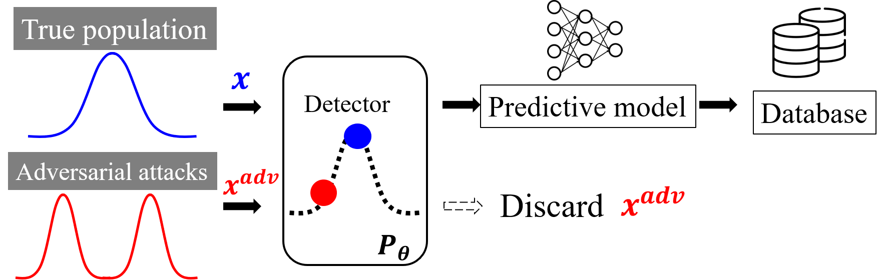
However, detecting adversarial examples may be as crucial as defending them in certain applications, in which alerting the victim of an existence of adversarial samples suffices. For instance, models used for automation of tasks (e.g. review sentiment analysis, news headline classification, etc) are adopted to efficiently gain information about the true data-generating population (e.g. consumers, news media, etc), rather than the adversary. For such applications, attaining outputs of an adversarial input - whether correct or not - may turn out to be harmful to the system. Accordingly, the discard-rather-than-correct strategy which simply discards the detected adversarial input would be a good countermeasure. Moreover, being able to detect adversarial examples may be a step towards building a more robust defense model as the popular defense paradigm, adversarial training, usually suffers from degraded performance on normal inputs (Bao et al., 2021). With a competent detection system, the normal and adversarial inputs can be processed by two separate mechanisms as proposed by Zhou et al. (2019).
| Method | Summary | Require Train Data? | Require Val. Data? | Target Attacks† |
| RDE (Ours) | Feature-based density estimation | Token-level | ||
| Mozes et al. (2021, FGWS) | Word frequency-based | ✓ | Word-level | |
| Bao et al. (2021, ADFAR) | Learning-based (sentence-level) | ✓ | ✓ | Word-level |
| Le et al. (2021, DARCY) | Learning-based (Honeypot) | ✓ | ✓ | Wallace et al. (2019) |
| Zhou et al. (2019, DISP) | Learning-based (token-level) | ✓ | ✓ | Token-level |
| Pruthi et al. (2019) | Learning-based (Semi-character RNN) | ✓ | ✓ | Char-level |
Many existing works that employ detection as an auxiliary task for defense require adversarial samples for training, which may be a restrictive scenario given the variety of attack methods and sparsity of adversarial samples in the real world. In addition, some works either focus on a single type of attack (Le et al., 2021) or is limited to character-level attacks (Pruthi et al., 2019), both of which do not abide the two key constraints (semantics and grammaticality) in order to be imperceptible (Morris et al., 2020a). As opposed to this, carefully crafted word-level adversarial attacks can maintain original semantics and remain unsuspicious to human inspectors. To encourage further research in this domain, we release a benchmark for word-level adversarial example detection on four attack methods across four NLP models and four text classification datasets. We also propose a simple but effective detection method that utilizes density estimation in the feature space as shown in Fig. 1 without any assumption of the attack algorithm or requiring adversarial samples for training or validation. We summarize the existing works in Table 1.
As opposed to a recent work (Mozes et al., 2021), which relies on word frequency to assess the likelihood of sentence(s), we model the probability density of the entire sentence(s). To achieve this, we fit a parametric density estimation model to the features obtained from a classification model (e.g. BERT) to yield likelihoods of each sample as shown by Fig. 2 inspired by classic works in novelty detection (Bishop, 1994), which utilizes generative models to find anomalies. However, simply fitting a parametric model suffers from curse of dimensionality characterized by (i) sparse data points and spurious features (ii) and rare outliers that hamper accurate estimation. To tackle these issues, we leverage classical techniques in statistical analysis, namely kernel PCA and Minimum Covariance Determinant, for robust density estimation (RDE).

Our attack-agnostic and model-agnostic detection method achieves the best performance as of auc on 29 out of 30 dataset-attack-model combinations and best performance as of tpr, f1 , auc on 25 of them without any assumption on the attacks.
Our contributions are two-fold:
-
•
We propose a adversarial detection method that does not require validation sets of each attack method through robust parameter estimation.
-
•
We release a dataset for word-level adversarial example detection on 4 attacks, 4 text classification datasets, and 4 models and the source code for experimenting on various experimental protocols.
We further provide analysis on a stronger adversary with partial knowledge of the detection method and techniques to counteract the adversary. Last, we investigate the proposed method’s applicability on character-level attacks.
| Dataset | Topic | Task | Classes | Median Length | # of Test Samples Original / Generated |
| IMDB(Maas et al., 2011) | movie review | sentiment classification | 2 | 161 | 25K / 10K |
| AG-News(Zhang et al., 2015) | news headline | topic classification | 4 | 44 | 7.6K / 7.6K |
| SST-2(Socher et al., 2013) | movie review | sentiment classification | 2 | 16 | 2.7K / 2.7K |
| YELP(Zhang et al., 2015) | restaurant review | sentiment classification | 2 | 152 | 38K / 5K |
2 Preliminaries
2.1 Adversarial Examples
Given an input space , a label space , a predictive model , and an oracle model , a successful adversarial example of an input satisfies the following:
| (1) |
where is an indicator function for the -th constraint between the perturbed text and the original text, which is 1 when the two texts are indistinguishable with respect to the constraint. The constraints vary from attack algorithms and is crucial for maintaining the original semantics while providing an adequate search space. For instance, Jin et al. (2020) ensure that the embedding of the two sentences have a cosine similarity larger than 0.5 using the Universal Sentence Encoder (Cer et al., 2018, USE).
2.2 Detecting Adversarial Examples
For the purpose of detecting adversarial examples, a dataset, , consisting of clean samples () and adversarial samples () is required. However, how the dataset should be configured has rarely been discussed in detail and the exact implementation varies by works. Here we discuss two main configurations used in the literature. We denote the test set as and the correctly classified test set as .
-
Scenario 1 : Sample disjoint subsets , . For the correctly classified examples of , adversarial attacks are generated and the successful examples form . is formed from .
-
Scenario 2 : Sample subset . For the correctly classified examples of , adversarial attacks are generated and the successful examples form . is formed from .
Scenario 1 provides more flexibility in choosing the ratio between adversarial samples and clean samples, while in Scenario 2 this is determined by the attack success rate and task accuracy. For instance, an attack with a low success rate will have a low adversarial-to-clean sample ratio. In addition, Scenario 2 consists of pairs of adversarial samples and their corresponding clean sample in addition to the incorrect clean samples. A more challenging scenario can be proposed by including failed attacked samples, which may be closer to the real world.
A seminal work (Xu et al., 2018) on adversarial example detection in the image domain assumes the first scenario, whereas existing works in NLP Le et al. (2021); Mozes et al. (2021) only experiment on the second scenario. Our benchmark framework provides the data and tools for experimenting on both. We provide experiment results on both scenarios.
3 Method
3.1 Benchmark
We generate adversarial examples on 4 models, 4 types of attacks, and 4 sentence classification datasets. Since some attacks (Garg and Ramakrishnan, 2020) require hundreds of queries and inference of models per query, vast amount of time is required to create all the adversarial examples (e.g. up to 44 hours for 5,000 examples on the IMDB dataset using TF-adjusted attack). This renders on-the-fly generation and detection of adversarial examples extremely inefficient. Therefore, adversarial examples are created beforehand and sampled according to Section 2.2. Four sentence classification datasets (IMDB, AG-News, SST-2, Yelp) are chosen to have diverse topics and length. See Table 2 for the summary and the number of generated samples.
We choose two non-transformer-based models (Word-CNN Kim (2014); LSTM Hochreiter and Schmidhuber (1997)) and two transformer-based models (RoBERTa Liu et al. (2019); BERT Devlin et al. (2018)) . Recently, numerous adversarial attacks have been proposed. We choose two widely known attacks called Textfooler (Jin et al., 2020, TF) and Probability Weighted Word Saliency (Ren et al., 2019, PWWS) and a recent approach using BERT to generate attacks called BAE (Garg and Ramakrishnan, 2020). Lastly, we also include a variant of TF called TF-adjusted (Morris et al., 2020a, TF-adj), which enforces a stronger similarity constraint to ensure imperceptibility to humans. All attacks are created using the TextAttack library (Morris et al., 2020b). See Appendix A.1 for the summary of attack methods and Appendix A.5 for a code snippet of using our benchmark.
3.2 Estimating Density and Parameters in Feature Space

Earlier works in novelty detection (Bishop, 1994) have shown that generative models fitted on normal samples are capable of detecting unseen novel samples (e.g. adversarial samples). Since we can assume that the training samples, which were used to train the victim model of a particular task, are available to the victim party, we can similarly design a generative model that estimates input density. However, directly using the inputs is challenging as modeling the probability distribution of raw texts is non-trivial. To bypass this, we fit a parametric density estimation model in the feature space (i.e. penultimate layer of the classification model). Since a neural network learns to extract important features of the inputs to distinguish classes, the features can be regarded as representations of the raw inputs. For a pre-trained predictive model , let denote the feature given by the feature extractor . Then the entire predictive model can be written as the composition of and a linear classifier.
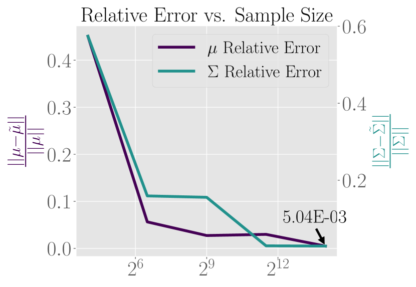
Given a generative model with mean and covariance as parameters , we can use the features of the training samples () to estimate the parameters. Then, novel adversarial samples lying in the unobserved feature space are likely to be assigned a low probability, because the generative model only used the normal samples for parameter fitting. For simplicity, we assume the distributions of the feature follow a multivariate Gaussian, and thus we model the class conditional probability as , where indicates the class of a given task. Then, the maximum likelihood estimate (MLE) is given by the sample mean and sample covariance .
However, accurate estimation of the parameters is difficult with finite amount of samples especially in high dimensions ( for transformer-based models) due to curse of dimensionality, thereby (i) leading to sparse data points and spurious features (ii) and occasional outliers that influence the parameter estimates. In Figure 3, we empirically show that the covariance matrices (blue) of BERT and RoBERTa across all models across all datasets are ill-conditioned, demonstrated by the high maximum eigenvalues and extremely small minimum eigenvalues (). Due to this, the precision matrix is abnormally inflated in certain dimensions and prone to numerical errors during inversion. More analysis regarding the upperbound of this error is provided in Appendix A.2.
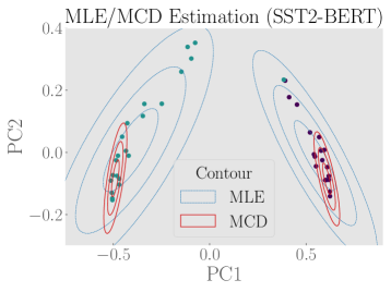
In addition, although we have assumed a Gaussian distribution for convenience, the unknown true distribution may be a more general elliptical distribution with thicker tails. This is observed empirically in Figure 4 by visualizing the features into two dimensions by dimensionality reduction. Outliers that are far from the modes of both classes (indicated by color) are present: those that are completely misplaced occasionally exist, while subtle outliers that deviate from the Gaussian distribution assumption are common, which influences the MLE estimation. Thus, to accurately estimate the Gaussian parameters, these outliers should be taken into account. In the following subsection, we tackle these issues through well-known classical techniques from statistical analysis.
3.3 RDE using kPCA and Minimum Covariance Determinant
To address the first issue, we first use kernel PCA (Schölkopf et al., 1998, kPCA) to select top orthogonal bases that best explain the variance of the data, thereby reducing redundant features. Given centered samples , a mapping function , and its mapping applied to each sample , kPCA projects the data points to the eigenvectors with the largest eigenvalues of the covariance 222For simplicity, we assume is centered. When this assumption does not hold, slightly modified approach is taken. See Appendix B of Schölkopf et al. (1998) for details.. Intuitively, this retains the most meaningful feature dimensions, which explains the data the most, while reducing spurious features and improve stability of inversion by decreasing the condition number as shown in Figure 3. By leveraging non-linear , we are able to find meaningful non-linear signals in the features as opposed to standard PCA. We use the radial basis function as our kernel. Comparison of performance with standard PCA is provided in Appendix Table A.5. For a complete derivation, please refer to Schölkopf et al. (1997).
However, this does not remove sample-level outliers as shown in Figure 4. Since we have assumed a Gaussian distribution, "peeling off" outliers may be favorable for parameter estimation. A principled way of removing outliers for parameter estimation has been an important research area in multivariate statistics and various methods have been developed for robust covariance estimation (Friedman et al., 2008; Ledoit and Wolf, 2004). Among them, Minimum Covariance Determinant (Rousseeuw, 1984, MCD) finds a subset of samples that minimizes the determinant of .333Although the possible number of subsets is infeasibly large, Rousseeuw and Driessen (1999) propose an iterative method that converges relatively fast for 4000 samples with 100 dimensions. As the determinant is proportional to the differential entropy of a Gaussian up to a logarithm (shown in Appendix A.3), this results in a robust covariance estimation consisting of centered data points rather than outliers. For a review, see Hubert et al. (2018). Qualitatively, we observe in Figure 4 that MLE estimates have their means yanked towards the outliers and that the contours are disoriented (Blue). MCD estimates (Red) focus on the high density clusters, which leads to higher performance as will be shown in the experiments.
In summary, we retain informative features by applying kPCA and obtain robust covariance estiamte by using MCD on the train set. Using the estimated robust parameters, we can evaluate the likelihood of a test sample. We treat those with low likelihood as novel (adversarial) samples. Our algorithm is shown in Algorithm 1 in the Appendix. We empirically validate the effectiveness of two techniques and discuss the effect of hyper-parameter and in the following sections.
4 Experiments
4.1 Experimental Settings
We experiment on the four datasets (IMDB, AG-News, SST-2, Yelp) and four attack methods described in Section 3.1. Our experiment is based on BERT and RoBERTa as they are widely used competent models for various tasks. Since SST-2 only has 1.8K test samples, TF-adjusted attack was unable to create an adequate number of successful adversarial samples (e.g. 80 samples out of 1.7K). Omitting experiments for these, there are 30 combinations of dataset-attack-model in total.
In addition, we (i) investigate a potential adversary with partial/full knowledge of the detection method (§4.6) and (ii) conduct experiments on a character level attack (Appendix A.9) to demonstrate the applicability of our method. Last, we discuss more realistic scenarios for further study and conduct hyper-parameter and qualitative analysis (§4.7).
4.2 Compared Methods
We compare our robust density estimation method (RDE) with a recently proposed detection method in NLP called FGWS (Mozes et al., 2021) which is a word frequency-based method that assumes that rare words appear more often in adversarial samples. We also verify whether Perplexity (PPL) computed by a language model (GPT-2, Radford et al. 2019) is able to distinguish normal and adversarial samples as PPL is often used to compare the fluency of the two samples. FGWS implicitly models the input density via word frequencies, while GPT-2 explicitly computes the conditional probability via an auto-regressive tasks. In addition, we adopt Lee et al. (2018) denoted as MLE, which is a out-of-distribution detector from the image domain. Similar to RDE, Lee et al. (2018) fits a Gaussian model using the maximum likelihood estimation (MLE) then trains a logistic regressor using the likelihood scores. Since we assume that adversarial samples are not available for training, we do not train a regression model, but only use the likelihood score. For further details, see Section 5. We compare MLE with two variants of our method:
-
•
RDE(-MCD) : This is a variant of RDE, in which only kPCA is applied to the features without MCD. The results of applying standard PCA instead of kPCA are reported in Table A.5 of Appendix.
-
•
RDE : After applying kPCA, MCD estimate is used. This is the final proposed robust density estimation incorporating both kPCA and MCD.
Models Methods Attacks TF PWWS BAE TF-adj tpr F1 auc tpr F1 auc tpr F1 auc tpr F1 auc IMDB BERT PPL 48.70.2 61.40.2 76.90.2 37.80.5 51.20.5 71.70.2 27.00.5 39.40.5 67.30.1 24.50.8 36.51.0 67.90.3 FGWS 84.60.3 87.10.2 87.10.3 88.20.1 89.00.0 90.80.0 62.10.3 72.30.2 70.90.3 72.60.9 80.60.9 78.40.6 MLE 86.31.1 87.90.7 94.50.2 75.71.4 81.50.9 92.40.2 81.81.3 85.30.8 93.70.2 88.31.0 89.10.6 95.30.2 RDE(-MCD) 96.30.3 93.40.2 96.80.1 86.90.9 88.30.5 94.60.2 92.50.5 91.40.3 95.80.2 98.20.2 94.60.2 97.60.2 RDE 96.60.2 93.50.1 97.70.2 87.80.4 88.80.2 95.20.2 93.80.1 92.10.0 96.90.2 98.80.0 95.00.1 98.70.2 RoBERTa PPL 47.80.1 60.60.1 78.40.1 43.50.7 56.70.6 76.10.2 25.90.4 38.20.5 67.00.2 26.60.9 39.01.1 69.10.4 FGWS 85.10.1 87.40.1 88.00.1 92.10.2 91.40.2 93.60.2 61.50.2 71.80.1 70.30.1 69.20.4 78.00.1 75.40.2 MLE 80.51.0 84.50.6 94.00.2 76.81.3 82.20.8 93.30.2 75.51.5 81.40.9 93.10.3 86.42.3 88.01.3 95.30.7 RDE(-MCD) 98.50.1 94.50.1 97.90.1 95.00.3 92.70.2 96.70.1 95.40.4 93.00.2 97.00.2 98.60.4 94.80.2 98.10.4 RDE 98.90.1 94.70.0 98.60.1 95.20.1 92.80.1 97.20.1 95.30.2 92.90.1 97.60.1 98.80.4 95.90.6 99.00.2 AG-News BERT PPL 75.70.4 81.60.2 91.00.2 70.80.7 78.30.5 89.50.2 31.21.3 44.21.4 73.00.8 32.81.8 45.91.9 73.30.8 FGWS 82.40.6 85.70.3 84.20.7 91.00.1 90.60.1 90.80.3 64.30.9 73.80.6 71.30.4 63.81.0 74.31.0 71.90.7 MLE 77.80.5 82.90.3 93.50.1 70.40.9 78.00.6 92.00.1 72.71.8 79.61.2 92.80.4 71.01.6 78.90.9 92.00.2 RDE(-MCD) 96.20.1 93.30.0 97.10.1 89.80.8 90.00.4 95.60.1 93.20.9 92.10.6 96.20.3 96.61.0 93.60.5 96.00.1 RDE 95.80.2 93.20.1 96.90.1 88.71.0 89.30.6 95.40.1 96.60.1 93.70.1 96.90.1 98.20.6 95.40.3 97.50.3 RoBERTa PPL 77.10.5 82.40.3 91.80.1 72.20.8 79.30.5 89.60.2 37.11.4 50.41.5 74.70.3 31.81.3 45.31.3 74.31.3 FGWS 78.80.5 83.50.3 82.20.2 86.60.4 88.10.2 87.90.3 53.33.4 65.12.7 63.52.0 58.93.4 69.72.6 70.10.9 MLE 82.50.3 85.70.2 94.10.1 78.60.5 83.40.3 92.90.2 68.13.1 76.32.2 91.50.7 65.02.3 74.41.7 91.20.2 RDE(-MCD) 90.50.5 90.30.3 96.10.1 84.11.2 86.60.7 94.80.2 77.84.1 82.62.6 93.90.5 82.62.7 85.91.5 94.50.4 RDE 92.90.3 91.60.2 95.70.1 84.50.8 86.90.5 93.90.2 89.32.3 89.61.3 95.30.5 94.40.7 92.60.4 96.00.3 SST-2 BERT PPL 31.70.6 44.80.6 73.10.3 29.21.3 41.91.4 73.40.4 22.21.6 33.52.0 67.00.5 FGWS 60.80.4 72.30.3 73.60.3 79.90.6 84.90.4 86.70.4 34.70.3 48.00.3 60.30.3 MLE 33.31.3 46.51.4 79.80.5 23.20.4 34.80.6 78.40.3 32.61.3 45.81.5 76.80.6 RDE(-MCD) 61.30.8 71.60.6 86.30.4 46.60.7 59.50.6 84.60.2 45.41.3 58.51.1 80.60.6 RDE 66.10.8 75.10.5 87.70.3 54.31.1 66.10.9 86.60.2 48.01.4 60.71.2 81.00.5 RoBERTa PPL 34.70.7 48.00.7 75.00.5 32.51.6 45.51.7 73.90.5 20.01.3 30.81.6 65.30.4 FGWS 61.60.2 73.00.1 73.70.1 80.80.2 85.60.1 86.40.2 36.11.0 49.41.1 60.00.6 MLE 44.20.6 57.30.5 84.40.3 33.10.8 46.30.8 81.90.4 37.10.5 50.50.5 77.90.4 RDE(-MCD) 63.20.2 73.00.1 87.80.1 53.10.7 65.10.6 85.40.2 45.70.7 58.70.7 79.30.3 RDE 74.10.3 80.60.2 90.40.1 67.71.1 76.20.8 89.10.0 52.00.3 64.30.3 80.60.1
4.3 Evaluation Metric and Protocol
Following Xu et al. (2018), we report three widely used metrics in adversarial example detection : (1) True positive rate (tpr) is the fraction of true adversarial samples out of predicted adversarial samples. (2) F1-score (f1) measures the harmonic mean of precision and recall. Since all compared methods are threshold-based methods, we report tpr at a fixed false positive rate (fpr). (3) Area under ROC (auc) measures the area under tpr vs. fpr curve. For all three metrics, higher denotes better performance.
Note that whereas auc considers performance on various fpr’s, tpr and F1 is dependent on one particular fpr. In all our experiments, we fixed fpr, which means of normal samples are predicted to be adversarial samples. This threshold should be chosen depending on the context (i.e. the degree of safety-criticalness). We believe this standard should be elevated as more works are proposed in the future. For IMDB and AG-News, 30% of the test set is held out as validation set for Mozes et al. (2021). We subsample out of the test set as described in Section 2.2. For quantitative analysis, we report the mean and its standard error of three repetitions of random seeds for test/validation split and subsampled samples.
4.4 Implementation Details
We choose the feature to be the output of the last attention layer (before Dropout and fully connected layer) for BERT and RoBERTa. RDE has two main hyper-parameters, namely the number of retained dimensions of kPCA and the support fraction of MCD. We fix for all experiments as we observe the performance is not sensitive to . For , we use the default value proposed in the algorithm, which is . We study the effect of in Section 4.7. All models are pre-trained models provided by TextAttack and both kPCA and MCD are implemented using scikit-learn (Pedregosa et al., 2011). We use the radial basis function as our kernel. The time required to estimate the parameters of our method is approximately around 25 seconds. For more details, see Appendix A.4.
For FGWS, we use the official implementation444https://github.com/maximilianmozes/fgws and use the held-out validation set of each attack to tune the threshold for word frequency as done in the original work. For PPL, we use the HuggingFace (Wolf et al., 2020) implementation of GPT-2 (Radford et al., 2019).
4.5 Results on Static Adversary
Table 3 demonstrates the results on three datasets and four attacks. Results on Yelp are presented in Appendix Tab. A.6 . The highest means out of the four methods are written in bold. Out of the 30 combinations of dataset-attack-model, RDE achieves the best performance on 29 of them on auc and 25 of them for all three metrics, which shows the competitiveness of our simple method. The motivation of our method is verified by the large margin of improvement from MLE in almost all cases. Using MCD estimation also further improves performance except in the few cases of AG-News. Large language models (PPL) are able to distinguish between adversarial samples and normal samples in expectation as shown by the higher-than-random metric, but the performance is inadequate to be used as a detector. FGWS generally has higher performance compared to PPL, but is inferior to MLE in most cases. Note the degradation of performance in FGWS for BAE and TF-adj, which are more subtle attacks with stronger constraints, as FGWS relies on the use of rare words. This trend is not observed in feature density-based methods (MLE and RDE).
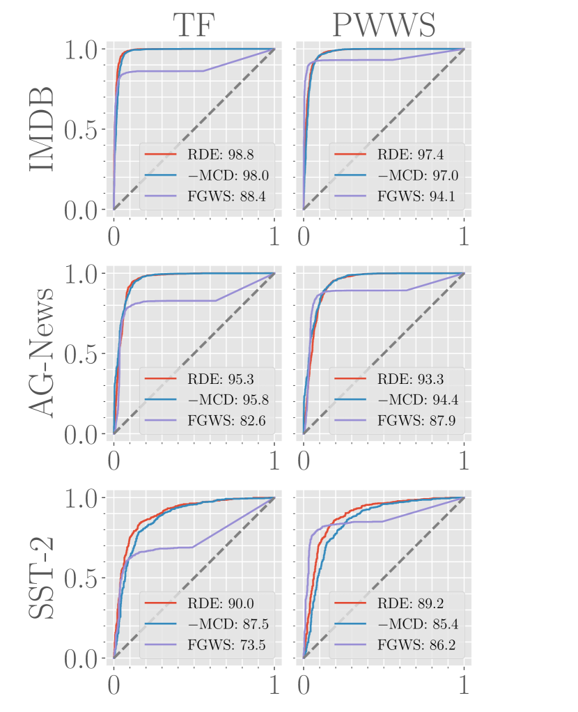
FGWS outperforms ours on tpr and F1 in five combinations out of 30, but our method has higher auc on four of them. Interestingly, all five results are from PWWS attacks, which indicates that our method is relatively susceptible to PWWS. Nonetheless, auc still remains fairly high: On IMDB and AG-News, the auc’s are all over 0.9. On the other hand, all methods have degraded performance on SST-2, which may be due to shorter sentence lengths. Some examples of ROC curves are presented in Appendix A.7. Improving detection rate in SST-2 is left as future work.
4.6 Results on Stronger Adversaries
Adaptive Adversary
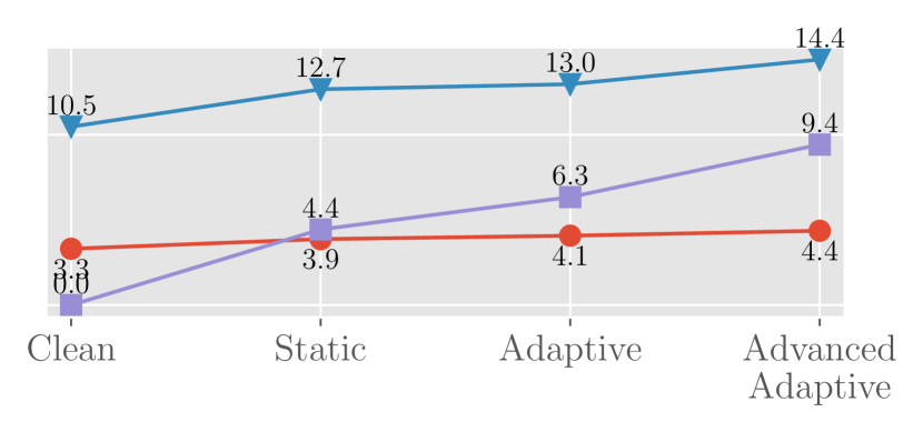
In this section, we assume that the adversary is aware of the detection method, but does not have full access to the model parameters. Being conscious of the fact that RDE relies on the discriminative feature space, the adversary does not terminate once the attacked sample reaches the decision boundary, but goes on to generate samples that are closer to the feature space of the incorrect target until a given threshold. Such attacks that increase the number of trials have been similarly applied in Xie et al. (2019) to create stronger attacks. As shown in Tab. 4, feature-based methods including RDE show considerable degradation in performance against these attacks, while PPL and FGWS have increased performance. All standard errors are less than 0.3.
TF-Strong PWWS-Strong BERT RoBERTa BERT RoBERTa Reference 97.7 98.6 95.2 97.2 PPL 79.0(+2.1) 84.4(+6.0) 73.7 (+2.0) 81.7 (+5.6) FGWS 87.9(+0.8) 90.5(+2.5) 92.2(+1.4) 95.3(+1.7) MLE 93.0(-1.5) 90.4(-3.6) 90.7(-1.7) 90.1(-3.2) RDE 94.7(-3.0) 92.9(-5.0) 92.4(-2.8) 92.0(-5.2) RDE+ 95.6 94.5 94.2 94.5
However, to combat these types of attacks, the defender can use a few examples of the previously detected static adversarial samples to adjust the feature space. Specifically, the features of the predictive model (e.g. BERT) are finetuned such that the adversarial samples are located near the decision boundary and far from the classes. To achieve this, the parameters of the predictive model are trained such that the entropy of the softmax probability can be maximized.
| (2) |
With only T=5 iterations and 80 adversarial samples (=16), RDE+ is able to recover some of its performance by adjusting the feature space. Since only a few updates are made to the model, the original task performance is negligibly affected (For RoBERTa, 95.1% is marginally increased to 95.2%).555For more details regarding the experiment, see the appendix. Note that only the previously detected static adversarial samples are used to finetune the feature space not the stronger attacks from the adaptive adversary. In addition, stronger attacks are usually more perceptible as it perturbs more words and cost more queries. For instance, on RoBERTa-TF, the average number of queries to the model per sample increasees from 625 786.
Advanced Adaptive / Oracle Adversary
If the adversary has full access to the model parameters, the adversary can easily generate attacks that can evade the detection method by iteratively attacking the likelihood score of RDE. We generate an even stronger attack than the adaptive adversary (advanced adaptive) such that the attacked sample is completely misclassified to the incorrect target to approximate the oracle adversary. However, we show in Figure 5 that such contrived attacks evade RDE at a cost of high perceptibility (grammatical error, PPL, semantic defect), rendering them detectable by human inspectors or other detection methods not reliant on the neural features.
4.7 Discussion
More Realistic Scenarios In previous experiments, all failed adversarial attacks were discarded. However, in reality an adversary will probably have no access to the victim model so some attacks will indeed fail to fool the model and have unbalanced clean to adversarial samples. In Appendix A.10, we discuss these scenarios and provide preliminary results.
Hyper-parameter Analysis Although the two main hyper-parameters, support fraction () of MCD and the dimension (), were fixed in our experiments, they can be fine-tuned in a separate validation set for optimal performance. We show in Figure 6 the performance of our method on various ranges of and on the validation set of IMDB-TF-BERT combination. We set and to the default value of the algorithm when tuning for the other parameter.
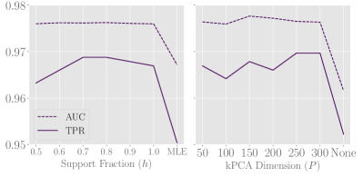
Qualitative Analysis on Support Fraction The support fraction controls the ratio of original samples to be retained by the MCD estimator, thereby controlling the volume of the contour as shown in Figure 7. We empirically demonstrated in our experiment that using all samples for parameter estimation may be detrimental for adversarial sample detection.

5 Related Works
Detection of adversarial examples is a well-explored field in the image domain. Earlier works have tackled in various ways such as input transformation (Xu et al., 2018), statistical analysis (Grosse et al., 2017), or training a separate binary classifier (Metzen et al., 2017). However, Carlini and Wagner (2017) has shown that an adversary with partial knowledge of the detector can easily nullify it. Meanwhile, early works in novelty detection have shown that a generative model can detect anomaly samples (Bishop, 1994). Following this line of research, Lee et al. (2018) have proposed a method to detect out-of-distribution samples by training a logistic regressor on features of a neural network for maximum likelihood estimation.
In the NLP domain, few efforts have been made in detecting word-level adversarial examples. Zhou et al. (2019, DISP) utilize a detector trained on adversarial samples for a joint detect-defense system. FGWS (Mozes et al., 2021) outperforms DISP in detection by building on the observation that attacked samples are composed of rare words on 2 attack methods. Le et al. (2021) tackle a particular attack method called UniTrigger (Wallace et al., 2019), which pre-pends or appends an identical phrase in all sentences. While the performance is impressive, applying this method to other attacks requires significant adjustment due to the distinct characteristics of UniTrigger. Meanwhile, Pruthi et al. (2019) tackle character-level adversarial examples and compare with spell correctors. Our work is the first to extensively demonstrate experimental results for 4 popular and recent attack methods on 4 datasets and propose a competitive baseline. We summarize the methods in Tab. 1.
6 Conclusion
We propose a general method and benchmark for adversarial example detection in NLP. Our method RDE does not require training or validation sets for each attack algorithms, yet achieves competitive performance. In the future, a principled coutermeausre for an adversary with partial or full knowledge can be considered for robustness.
References
- Anderson (1962) Theodore Wilbur Anderson. 1962. An introduction to multivariate statistical analysis. Technical report, Wiley New York.
- Bao et al. (2021) Rongzhou Bao, Jiayi Wang, and Hai Zhao. 2021. Defending pre-trained language models from adversarial word substitutions without performance sacrifice. arXiv preprint arXiv:2105.14553.
- Bishop (1994) C.M. Bishop. 1994. Novelty detection and neural network validation. IEEE Proceedings - Vision, Image and Signal Processing, 141:217–222(5).
- Carlini and Wagner (2017) Nicholas Carlini and David Wagner. 2017. Adversarial examples are not easily detected: Bypassing ten detection methods. In Proceedings of the 10th ACM workshop on artificial intelligence and security, pages 3–14.
- Cer et al. (2018) Daniel Cer, Yinfei Yang, Sheng-yi Kong, Nan Hua, Nicole Limtiaco, Rhomni St John, Noah Constant, Mario Guajardo-Céspedes, Steve Yuan, Chris Tar, et al. 2018. Universal sentence encoder. arXiv preprint arXiv:1803.11175.
- Devlin et al. (2018) Jacob Devlin, Ming-Wei Chang, Kenton Lee, and Kristina Toutanova. 2018. Bert: Pre-training of deep bidirectional transformers for language understanding. arXiv preprint arXiv:1810.04805.
- Friedman et al. (2008) Jerome Friedman, Trevor Hastie, and Robert Tibshirani. 2008. Sparse inverse covariance estimation with the graphical lasso. Biostatistics, 9(3):432–441.
- Garg and Ramakrishnan (2020) Siddhant Garg and Goutham Ramakrishnan. 2020. Bae: Bert-based adversarial examples for text classification. In Proceedings of the 2020 Conference on Empirical Methods in Natural Language Processing (EMNLP), pages 6174–6181.
- Grosse et al. (2017) Kathrin Grosse, Praveen Manoharan, Nicolas Papernot, Michael Backes, and Patrick McDaniel. 2017. On the (statistical) detection of adversarial examples. arXiv preprint arXiv:1702.06280.
- Hochreiter and Schmidhuber (1997) Sepp Hochreiter and Jürgen Schmidhuber. 1997. Long short-term memory. Neural computation, 9(8):1735–1780.
- Hubert et al. (2018) Mia Hubert, Michiel Debruyne, and Peter J Rousseeuw. 2018. Minimum covariance determinant and extensions. Wiley Interdisciplinary Reviews: Computational Statistics, 10(3):e1421.
- Jin et al. (2020) Di Jin, Zhijing Jin, Joey Tianyi Zhou, and Peter Szolovits. 2020. Is bert really robust? a strong baseline for natural language attack on text classification and entailment. In Proceedings of the AAAI conference on artificial intelligence, volume 34, pages 8018–8025.
- Jones et al. (2020) Erik Jones, Robin Jia, Aditi Raghunathan, and Percy Liang. 2020. Robust encodings: A framework for combating adversarial typos. In Proceedings of the 58th Annual Meeting of the Association for Computational Linguistics, pages 2752–2765.
- Keller et al. (2021) Yannik Keller, Jan Mackensen, and Steffen Eger. 2021. BERT-defense: A probabilistic model based on BERT to combat cognitively inspired orthographic adversarial attacks. In Findings of the Association for Computational Linguistics: ACL-IJCNLP 2021, pages 1616–1629, Online. Association for Computational Linguistics.
- Kim (2014) Yoon Kim. 2014. Convolutional neural networks for sentence classification. CoRR, abs/1408.5882.
- Le et al. (2021) Thai Le, Noseong Park, and Dongwon Lee. 2021. A sweet rabbit hole by darcy: Using honeypots to detect universal trigger’s adversarial attacks. In 59th Annual Meeting of the Association for Comp. Linguistics (ACL).
- Ledoit and Wolf (2004) Olivier Ledoit and Michael Wolf. 2004. A well-conditioned estimator for large-dimensional covariance matrices. Journal of multivariate analysis, 88(2):365–411.
- Lee et al. (2018) Kimin Lee, Kibok Lee, Honglak Lee, and Jinwoo Shin. 2018. A simple unified framework for detecting out-of-distribution samples and adversarial attacks. Advances in neural information processing systems, 31.
- Li et al. (2020) Linyang Li, Ruotian Ma, Qipeng Guo, Xiangyang Xue, and Xipeng Qiu. 2020. Bert-attack: Adversarial attack against bert using bert. In Proceedings of the 2020 Conference on Empirical Methods in Natural Language Processing (EMNLP), pages 6193–6202.
- Liu et al. (2019) Yinhan Liu, Myle Ott, Naman Goyal, Jingfei Du, Mandar Joshi, Danqi Chen, Omer Levy, Mike Lewis, Luke Zettlemoyer, and Veselin Stoyanov. 2019. Roberta: A robustly optimized bert pretraining approach. arXiv preprint arXiv:1907.11692.
- Maas et al. (2011) Andrew L. Maas, Raymond E. Daly, Peter T. Pham, Dan Huang, Andrew Y. Ng, and Christopher Potts. 2011. Learning word vectors for sentiment analysis. In Proceedings of the 49th Annual Meeting of the Association for Computational Linguistics: Human Language Technologies, pages 142–150, Portland, Oregon, USA. Association for Computational Linguistics.
- Metzen et al. (2017) Jan Hendrik Metzen, Tim Genewein, Volker Fischer, and Bastian Bischoff. 2017. On detecting adversarial perturbations. International Conference on Learning Representations.
- Morris et al. (2020a) John Morris, Eli Lifland, Jack Lanchantin, Yangfeng Ji, and Yanjun Qi. 2020a. Reevaluating adversarial examples in natural language. In Proceedings of the 2020 Conference on Empirical Methods in Natural Language Processing: Findings, pages 3829–3839.
- Morris et al. (2020b) John Morris, Eli Lifland, Jin Yong Yoo, Jake Grigsby, Di Jin, and Yanjun Qi. 2020b. Textattack: A framework for adversarial attacks, data augmentation, and adversarial training in nlp. In Proceedings of the 2020 Conference on Empirical Methods in Natural Language Processing: System Demonstrations, pages 119–126.
- Mozes et al. (2021) Maximilian Mozes, Pontus Stenetorp, Bennett Kleinberg, and Lewis Griffin. 2021. Frequency-guided word substitutions for detecting textual adversarial examples. In Proceedings of the 16th Conference of the European Chapter of the Association for Computational Linguistics: Main Volume, pages 171–186.
- Mrkšić et al. (2016) Nikola Mrkšić, Diarmuid O Séaghdha, Blaise Thomson, Milica Gašić, Lina Rojas-Barahona, Pei-Hao Su, David Vandyke, Tsung-Hsien Wen, and Steve Young. 2016. Counter-fitting word vectors to linguistic constraints. arXiv preprint arXiv:1603.00892.
- Pedregosa et al. (2011) F. Pedregosa, G. Varoquaux, A. Gramfort, V. Michel, B. Thirion, O. Grisel, M. Blondel, P. Prettenhofer, R. Weiss, V. Dubourg, J. Vanderplas, A. Passos, D. Cournapeau, M. Brucher, M. Perrot, and E. Duchesnay. 2011. Scikit-learn: Machine learning in Python. Journal of Machine Learning Research, 12:2825–2830.
- Princeton (2010) Princeton. 2010. Princeton university "about wordnet." wordnet.
- Pruthi et al. (2019) Danish Pruthi, Bhuwan Dhingra, and Zachary C Lipton. 2019. Combating adversarial misspellings with robust word recognition. In Proceedings of the 57th Annual Meeting of the Association for Computational Linguistics, pages 5582–5591.
- Radford et al. (2019) Alec Radford, Jeffrey Wu, Rewon Child, David Luan, Dario Amodei, Ilya Sutskever, et al. 2019. Language models are unsupervised multitask learners. OpenAI blog, 1(8):9.
- Ren et al. (2019) Shuhuai Ren, Yihe Deng, Kun He, and Wanxiang Che. 2019. Generating natural language adversarial examples through probability weighted word saliency. In Proceedings of the 57th annual meeting of the association for computational linguistics, pages 1085–1097.
- Rousseeuw (1984) Peter J Rousseeuw. 1984. Least median of squares regression. Journal of the American statistical association, 79(388):871–880.
- Rousseeuw and Driessen (1999) Peter J Rousseeuw and Katrien Van Driessen. 1999. A fast algorithm for the minimum covariance determinant estimator. Technometrics, 41(3):212–223.
- Schölkopf et al. (1997) Bernhard Schölkopf, Alexander Smola, and Klaus-Robert Müller. 1997. Kernel principal component analysis. In International conference on artificial neural networks, pages 583–588. Springer.
- Schölkopf et al. (1998) Bernhard Schölkopf, Alexander Smola, and Klaus-Robert Müller. 1998. Nonlinear component analysis as a kernel eigenvalue problem. Neural computation, 10(5):1299–1319.
- Socher et al. (2013) Richard Socher, Alex Perelygin, Jean Wu, Jason Chuang, Christopher D. Manning, Andrew Ng, and Christopher Potts. 2013. Recursive deep models for semantic compositionality over a sentiment treebank. In Proceedings of the 2013 Conference on Empirical Methods in Natural Language Processing, pages 1631–1642, Seattle, Washington, USA. Association for Computational Linguistics.
- Wallace et al. (2019) Eric Wallace, Shi Feng, Nikhil Kandpal, Matt Gardner, and Sameer Singh. 2019. Universal adversarial triggers for attacking and analyzing nlp. In Proceedings of the 2019 Conference on Empirical Methods in Natural Language Processing and the 9th International Joint Conference on Natural Language Processing (EMNLP-IJCNLP), pages 2153–2162.
- Wolf et al. (2020) Thomas Wolf, Lysandre Debut, Victor Sanh, Julien Chaumond, Clement Delangue, Anthony Moi, Pierric Cistac, Tim Rault, Rémi Louf, Morgan Funtowicz, Joe Davison, Sam Shleifer, Patrick von Platen, Clara Ma, Yacine Jernite, Julien Plu, Canwen Xu, Teven Le Scao, Sylvain Gugger, Mariama Drame, Quentin Lhoest, and Alexander M. Rush. 2020. Transformers: State-of-the-art natural language processing. In Proceedings of the 2020 Conference on Empirical Methods in Natural Language Processing: System Demonstrations, pages 38–45, Online. Association for Computational Linguistics.
- Xie et al. (2019) Cihang Xie, Yuxin Wu, Laurens van der Maaten, Alan L Yuille, and Kaiming He. 2019. Feature denoising for improving adversarial robustness. In Proceedings of the IEEE/CVF Conference on Computer Vision and Pattern Recognition, pages 501–509.
- Xu et al. (2018) Weilin Xu, David Evans, and Yanjun Qi. 2018. Feature squeezing: Detecting adversarial examples in deep neural networks. Network and Distributed Systems Security Symposium.
- Zhang et al. (2020) Wei Emma Zhang, Quan Z Sheng, Ahoud Alhazmi, and Chenliang Li. 2020. Adversarial attacks on deep-learning models in natural language processing: A survey. ACM Transactions on Intelligent Systems and Technology (TIST), 11(3):1–41.
- Zhang et al. (2015) Xiang Zhang, Junbo Zhao, and Yann LeCun. 2015. Character-level convolutional networks for text classification. Advances in neural information processing systems, 28:649–657.
- Zhou et al. (2021) Yi Zhou, Xiaoqing Zheng, Cho-Jui Hsieh, Kai-Wei Chang, and Xuan-Jing Huang. 2021. Defense against synonym substitution-based adversarial attacks via dirichlet neighborhood ensemble. In Proceedings of the 59th Annual Meeting of the Association for Computational Linguistics and the 11th International Joint Conference on Natural Language Processing (Volume 1: Long Papers), pages 5482–5492.
- Zhou et al. (2019) Yichao Zhou, Jyun-Yu Jiang, Kai-Wei Chang, and Wei Wang. 2019. Learning to discriminate perturbations for blocking adversarial attacks in text classification. In Proceedings of the 2019 Conference on Empirical Methods in Natural Language Processing and the 9th International Joint Conference on Natural Language Processing (EMNLP-IJCNLP), pages 4904–4913.
Appendix A Appendix
A.1 Success Rate of Attack Methods and Other Statistics
Here we briefly describe each attack method and provide some statistics about the attack results. For Table A.1, word transformation method indicates how candidate replacement words are created. Word importance ranking denotes how the ordering of which word to attack is chosen. For constraints, only those related to embedding was listed and the numbers in parenthesis denote the threshold. Higher threshold signifies stronger constraint. For more details, we refer the readers to Morris et al. (2020b). Table A.2 summarizes the attack results on three dataset for BERT. Results for other models can be found in the released dataset.
| Attacks | Citations | Word Transformation Method | Word Importance Ranking Method | Constraints |
| TF | 204 | Counter-fitted GLOVE (Mrkšić et al., 2016) | Delete Word | USE(0.84) WordEmbedding Distance(0.5) |
| PWWS | 187 | WordNet (Princeton, 2010) | Weighted Saliency | - |
| BAE | 71 | Bert Masked LM | Delete Word | USE(0.94) |
| TF-adj | 18 | Counter-fitted GLOVE | Delete Word | USE(0.98) WordEmbedding Distance(0.9) |
| Attacks | Post-Attack Accuracy | Attack Success Rate | Average Num. Queries |
| IMDB (91.9%) | |||
| TF | 0.6% | 99% | 558 |
| PWWS | 3% | 97% | 1681 |
| BAE | 34% | 64% | 455 |
| TF-adj | 84.2% | 11% | 298 |
| AG-News (94.2%) | |||
| TF | 18% | 81% | 334 |
| PWWS | 41% | 57% | 362 |
| BAE | 82% | 14% | 122 |
| TF-adj | 91% | 5% | 56 |
| SST-2 (92.43%) | |||
| TF | 4% | 96% | 91 |
| PWWS | 12% | 87% | 143 |
| BAE | 37% | 61% | 60 |
| TF-adj | 89% | 5% | 25 |
| Successful | director brian levant, who never strays far from his sitcom roots, skates blithely from one implausible[improbable] situation to another [..] |
|
| Failed | arnold ’s jump[leap] from little screen to big will leave frowns on more than a few faces |
|
A.2 Potential Errors of Parameter Estimation
Accurate estimation of the parameters is difficult with finite amount of samples especially in high dimensions. Here we demonstrate this through a toy example and derive its relationship with the Mahalanobis distance function, which is proportional to the likelihood. Figure A.1 shows that the MLE error remains high even when samples are used to find the parameters of a noise-free normal distribution for both and . This, in turn, leads to an inevitably error-prone and . Moreover, the error is amplified when computing the Mahalanobis distance due to the ill-conditioned with very small eigenvalues, which is observed empirically in all datasets and models (Figure 3) possibly due to the redundant features. The (relative) condition number of the Mahalanobis distance function - relative change in the output given a relative change in the inputs - is bounded by the inverse of the smallest eigenvalue of .
| (3) | ||||
where the first equality follows from the definition of condition number and differentiability of and . The last equality follows from the Caucy-Schwarz Inequality. The matrix norm induced by the L2 norm is given by the largest singular value (largest eigenvalue for a positive definite square matrix). Given the eigenspectrum of as , the eigenspectrum of is given by the reciprocal of that of Thus, is equal to inverse of the minimum eigenvalue of and the last equality can be further decomposed into
| (4) | ||||
where is a constant for a given . This means that when the smallest eigenvalue is in the scale of , even a estimation error of scale on may be amplified by at most by a scale of . This leads to a serious problem in density estimation of .
A.3 More details on MCD
We explain some of the properties of the determinant of the covariance matrix. First, the determinant is directly related to the differential entropy of the Gaussian distribution. For a -dimensional multivariate Gaussian variable and its probability density function , the differential entropy is given by
| (5) | ||||
In addition, the determinant is also proportional to the volume of the ellipsoid for some , . We refer the readers to Section 7.5 of Anderson (1962) for the proof. This explain why the MCD estimate forms a much narrower probability contour than MLE as shown in Fig. 4.
A.4 Implementation Details
To meet the memory constraint of computing the kernel matrix, we sample a subset of (8,000 samples) for all experiments. All models are pre-trained models provided by TextAttack and both kPCA and MCD are implemented using scikit-learn (Pedregosa et al., 2011). We use the radial basis function as our kernel.
For subsampling generated attacks described in Section 2.2, we set the maximum number of adversarial samples for each dataset. For IMDB and AG-News, the maximum is set to 2000 and for SST-2 this is set to 1000. Then, the number of target samples (i.e. ) is initialized to the maximum number divided by adversarial success ratio and task accuracy. Target sample is decremented until ratio between clean and adversarial samples can roughly be 5:5. Algorithm of RDE and MLE is provided in Algorithm 1.
A.5 Benchmark Usage Example

A.6 Comparison with PCA
In all our experiments, we used a radial basis function for kPCA. This allows finding non-linear patterns in the feature space. When the linear kernel is used, kPCA is equivalent to ordinary PCA. We demonstrate that exploiting non-linearity preserve much more meaningful information by comparing the detection performance in the IMDB dataset (Table A.5).
A.7 ROC Curve Examples
Below (Fig. A.3) we provide Receiver Operating Characteristic (ROC) curves of RoBERTa on two attacks. For all plots, samples from the first seed are used.
A.8 Experiment Details on Adaptive Adversary
In this section, we provide detail on the experimental settings. Instead of the terminating condition used by all attack methods
| (6) |
the stronger attack goes on to send the sample closer to the features of the incorrect target. With fixed , the attack terminates once
| (7) |
where is the largest predicted softmax probability. This allows the generated sample to fool the density-based methods that rely on the discriminative feature space. For attacks denoted ’strong’ ; for ’stronger’, . For RDE+, we use the adversarial samples of the held-out validation set using the static attack method.
A.9 Detecting Character-level Attacks
Although character level attacks are perceptible to spell checkers or more sophisticated techniques (Pruthi et al., 2019), it still poses threat to deep neural networks (Zhang et al., 2020). We demonstrate the general applicability of RDE on charcter-level attack on 3,000 samples attacked by the character-level attack method proposed in Pruthi et al. (2019). As shown in Table A.4, RDE surpasses all the density-based methods.
IMDB AG-News BERT RoBERTa BERT RoBERTa PPL 55.00.6 64.01.4 71.30.7 71.30.7 MLE 90.20.4 89.60.3 89.90.4 77.50.6 RDE 91.00.1 92.90.2 90.90.5 91.00.4
A.10 More Realistic Scenarios
In this section, we discuss more realistic scenarios and provide preliminary results in Appendix A.10: (i) Including failed attacks (ii) Imbalanced ratio of clean and adversarial samples. In previous experiments, all failed adversarial attacks were discarded. However, in reality an adversary will probably have no access to the victim model so some attacks will indeed fail to fool the model. While failed adversarial attacks do not pose threat to the task accuracy of the model, it nevertheless may be harmful if the victim wishes to gain information about a certain population by aggregating data such as sentiment in consumer review about a movie. In addition, as active research in attacks have been made in the past few years, more subtle attacks that are imperceptible to humans naturally have lower attack success ratio (e.g. BAE).
Fig. A.2 demonstrates the detection results of RDE and MLE when distinguishing between normal samples and (failed and successful) adversarial attempts by comparing the auc’s. As an upper bound, we provide the performance of RDE on the original scenario without failed adversarial examples in red. As the first two attacks (TF and PWWS) achieve nearly 100% success rate, only few failed adversarial samples are added. Accordingly, the performances for the two attacks show little difference. However, in more subtle attacks (BAE and TF-adj) the performance drastically drops due to the increased failed adversarial samples, yet RDE outperforms MLE by a considerable margin in most cases. We end on this topic by noting that more comprehensive analysis is called for, because in some cases failed adversarial attempts are (nearly) identical to clean samples. So an attack method with low detection rate does not necessarily imply a crafty attack method in this scenario.
In Appendix Table A.7, we provide the results for Scenario 2 described in Section 2.2. The general trend among detection methods and attack methods is similar to Table 3. As noted earlier, for Scenario 2 the ratio of adversarial to clean samples will be low if the attack success rate is low. For instance, in IMDB-(TF-adj)-BERT, the ratio of adversarial to clean samples is around 1:9. Whereas both auc and tpr are not strongly affected due to the characteristic of the metrics, F1 drastically drops. For instance, for IMDB-(TF-adj)-BERT, RDE achieves 73.7% (as opposed to 95.0% of Scenario 1). On the same set, FGWS achieves 60.1% and MLE achieves 67.6%.
Here we provide experimental results on Scenario 2. Although pairs of samples are included in the dataset, the general trend is similar to that of Scenario 1. For attack methods with low success rate, the adversarial to clean sample ratio is low, which affects the F1-score.
Models Methods Attacks TF PWWS BAE TF-adj tpr F1 auc tpr F1 auc tpr F1 auc tpr F1 auc BERT PCA 89.51.1 89.70.6 95.20.1 77.91.3 82.90.8 93.10.2 83.51.3 86.30.7 94.20.2 92.81.2 91.70.7 96.20.2 kPCA 96.30.3 93.40.2 96.80.1 86.90.9 88.30.5 94.60.2 92.50.5 91.40.3 95.80.2 98.20.2 94.60.2 97.60.2 RoBERTa PCA 94.70.6 92.50.3 96.30.1 89.70.9 89.90.5 95.40.1 88.21.3 89.00.7 95.00.3 92.61.8 91.60.9 96.70.5 kPCA 98.50.1 94.50.1 97.90.1 95.00.3 92.70.2 96.70.1 95.40.4 93.00.2 97.00.2 98.60.4 94.80.2 98.10.4
Models Methods Attacks TF PWWS BAE TF-adj tpr F1 auc tpr F1 auc tpr F1 auc tpr F1 auc BERT PPL 40.20.2 53.50.2 76.60.0 36.20.7 49.60.8 74.20.4 16.30.7 25.90.9 65.20.6 16.31.5 25.72.0 63.10.6 FGWS 84.60.5 87.20.2 87.00.5 88.90.1 89.50.1 91.00.0 62.41.2 72.50.8 70.30.8 79.72.7 85.51.7 82.30.8 MLE 41.31.0 54.61.0 66.50.3 41.80.8 55.00.8 66.90.2 42.31.9 55.51.8 67.50.4 38.52.1 52.02.0 66.70.8 RDE 97.90.1 94.30.1 96.40.0 92.70.5 91.50.3 94.90.1 97.10.2 94.00.1 96.20.1 99.80.1 95.70.1 96.40.1 RoBERTa PPL 38.50.7 51.80.7 73.00.5 36.30.8 49.60.9 71.70.6 17.00.6 26.70.7 60.60.7 12.71.2 20.81.7 58.60.5 FGWS 83.50.1 86.50.1 86.60.1 86.80.2 88.30.1 89.70.1 61.90.6 72.60.4 70.90.4 69.12.7 78.71.7 75.62.3 MLE 95.00.4 92.70.2 96.30.1 89.20.4 89.60.2 94.50.2 90.10.3 90.10.2 94.90.2 85.73.5 87.62.0 95.00.5 RDE 96.40.1 93.50.0 97.00.1 90.70.1 90.50.1 95.30.0 92.50.2 91.50.1 95.70.2 99.50.3 95.50.0 96.50.5
Models Methods Attacks TF PWWS BAE TF-adj tpr F1 auc tpr F1 auc tpr F1 auc tpr F1 auc IMDB BERT PPL 49.30.2 61.50.2 77.40.2 38.90.3 51.90.3 71.90.2 28.10.3 38.80.3 67.60.1 24.30.1 25.00.2 66.70.1 FGWS 82.60.1 85.40.1 85.10.1 86.60.1 87.70.1 89.30.1 60.60.2 68.50.2 69.30.2 71.30.2 60.10.2 76.60.1 MLE 86.41.2 87.60.7 94.60.1 76.11.7 81.31.1 92.60.2 82.00.6 82.60.3 93.70.1 87.00.2 67.60.2 95.00.0 RDE(-MCD) 96.00.4 92.80.2 96.60.1 86.20.8 87.50.5 94.40.1 92.10.3 88.30.2 95.60.1 98.50.0 73.40.0 97.50.0 RDE 96.80.2 93.20.1 97.70.1 87.40.5 88.10.3 95.10.2 93.30.3 89.00.1 96.80.1 98.80.0 73.70.1 98.60.0 RoBERTa PPL 49.50.4 61.80.3 78.90.3 45.10.2 57.90.2 76.50.2 26.90.1 37.90.1 67.60.1 26.60.4 21.30.3 68.10.3 FGWS 83.50.2 86.20.1 86.60.2 91.60.1 90.70.0 93.10.1 60.70.1 69.10.1 69.30.2 66.00.4 46.90.2 72.90.4 MLE 80.70.8 84.40.5 94.00.0 77.31.0 82.30.6 93.20.1 75.91.0 79.50.6 93.00.1 84.10.7 54.70.2 94.30.0 RDE(-MCD) 98.10.1 94.10.0 97.90.0 94.70.3 92.30.2 96.70.0 95.00.1 90.50.0 96.80.0 98.90.1 61.70.1 97.80.0 RDE 98.50.1 94.30.0 98.60.0 94.90.4 92.40.2 97.20.0 94.80.1 90.40.0 97.50.0 99.10.1 62.10.1 98.90.0 AG-News BERT PPL 76.30.3 80.70.2 91.30.1 72.40.4 75.80.3 90.20.1 30.60.5 29.90.4 72.80.2 35.00.5 19.80.2 74.30.4 FGWS 82.40.6 84.40.4 84.20.7 90.90.2 86.80.1 90.00.1 62.90.3 53.00.3 70.50.1 66.00.6 36.30.6 72.40.4 MLE 78.20.4 81.80.3 93.50.0 71.40.3 75.30.2 92.30.1 69.90.3 57.40.1 92.20.0 64.00.5 33.40.4 91.10.1 RDE(-MCD) 96.30.3 92.10.1 97.20.0 90.50.3 86.60.1 95.70.1 91.40.3 68.80.1 95.50.0 92.20.5 44.40.1 95.60.0 RDE 96.00.3 91.90.1 97.00.0 89.80.4 86.20.2 95.40.0 94.00.2 69.90.1 96.20.0 96.60.1 47.40.3 96.60.0 RoBERTa PPL 77.30.3 81.50.2 91.80.1 73.00.3 77.20.2 90.00.1 36.20.5 36.30.5 74.90.3 36.20.3 21.50.2 75.80.2 FGWS 79.60.4 83.00.2 82.60.3 86.60.3 85.50.2 88.00.2 52.70.4 48.90.3 64.60.5 60.70.7 34.40.3 70.20.3 MLE 81.40.2 84.10.1 94.00.1 78.70.0 80.80.0 93.10.0 68.40.2 59.10.2 91.70.1 62.60.2 34.30.2 90.00.0 RDE(-MCD) 89.90.3 89.00.2 96.10.0 85.80.5 85.00.3 95.10.1 81.40.2 66.60.2 94.40.1 80.40.1 42.00.2 93.70.0 RDE 92.70.2 90.50.1 95.60.0 86.40.3 85.40.2 94.20.1 92.60.2 72.30.2 95.70.0 93.60.1 47.60.4 95.70.0 SST-2 BERT PPL 33.40.5 46.20.6 73.10.1 30.40.5 42.60.5 73.10.0 22.20.1 31.70.1 65.70.0 FGWS 61.40.6 71.20.5 73.50.4 79.40.2 82.90.1 86.20.1 33.00.3 43.80.3 61.20.2 MLE 33.30.2 46.10.2 80.50.1 23.30.5 34.40.6 78.40.1 34.10.0 45.00.0 76.60.0 RDE(-MCD) 60.50.6 70.60.4 86.40.2 45.90.3 58.00.3 83.80.1 44.10.0 54.50.0 79.90.0 RDE 66.30.3 74.80.2 87.60.2 53.00.1 64.20.1 85.80.1 47.60.1 57.70.1 80.30.0 RoBERTa PPL 35.10.2 48.10.2 74.50.0 33.30.4 45.80.5 74.00.1 21.20.1 30.60.2 64.70.1 FGWS 61.40.4 71.20.3 73.70.2 80.10.3 83.40.2 86.20.1 36.70.4 47.70.4 60.50.1 MLE 41.80.3 54.70.2 84.20.1 31.60.4 44.00.4 81.50.2 37.00.0 48.00.0 77.70.0 RDE(-MCD) 62.50.6 72.10.5 87.50.3 51.90.6 63.30.5 84.70.1 45.60.3 56.10.2 79.20.1 RDE 73.30.6 79.60.4 90.40.2 65.70.3 73.90.2 88.50.1 50.90.1 60.60.1 80.20.1