Adaptive machine learning based surrogate modeling to accelerate PDE-constrained optimization in enhanced oil recovery

Abstract

In this contribution, we develop an efficient surrogate modeling framework for simulation-based optimization of enhanced oil recovery, where we particularly focus on polymer flooding. The computational approach is based on an adaptive training procedure of a neural network that directly approximates an input-output map of the underlying PDE-constrained optimization problem. The training process thereby focuses on the construction of an accurate surrogate model solely related to the optimization path of an outer iterative optimization loop. True evaluations of the objective function are used to finally obtain certified results. Numerical experiments are given to evaluate the accuracy and efficiency of the approach for a heterogeneous five-spot benchmark problem.

1 Introduction

Water flooding remains the most frequently used secondary oil recovery method. However, the percentage of original oil in place left after the cessation of water flooding in many reservoir fields is estimated to be as high as 50 - 70% [43, 34, 51]. The reduced performance of water flooding leading to the sizable leftover of oil has been linked to many factors such as the presence of unfavorable mobility ratios (due to heavy oil), high level of heterogeneity (in porosity and permeability), etc., in the reservoir [16]. For these reasons, enhanced oil recovery (EOR) methods are employed to improve the performance of water flooding in order to increase oil production and minimize environmental stress.

Polymer flooding is a matured chemical EOR method, suitable for heavy oil reservoir development, with over four decades of practical applications [1, 44]. It involves injecting long chains of high-molecular-weight soluble polymers along with water flooding. The polymer EOR mechanism includes reducing mobility ratios of the oil-water system and early water breakthrough in the reservoir by increasing the viscosity of injected water and consequently improving vertical and aerial sweep efficiencies of the injected fluid.

The EOR process of polymer flooding can significantly increase the oil production [44]. However, compared with water flooding, the operational cost and the risk associated with polymer flooding are higher. More so, since injecting more than necessary polymer into the reservoir can lead to insignificant oil increment, it is imperative to optimize the injection strategy of polymer flooding for field application to avoid unnecessarily high operational costs with no profit.

Conventionally, a reservoir simulation model is combined with a numerical optimization technique to determine an optimal control (including water rates, polymer concentrations of injection wells, liquid rates, or bottom hole pressures of production wells) for polymer flooding. The aim is to maximize a given reservoir performance measure (RPM), such as the total oil production or the net present value (NPV) function over the reservoir life. The simulation model is usually a complex numerical reservoir simulator that requires substantial data accounting for geology and geometry of the reservoir or rock and fluid properties. In this study, the model simulates the oil reservoir response (inform of fluid production) to a given polymer flooding control per time. On this account, we estimate the RPM of a given control strategy.

Further, the complexity of a reservoir simulator leads to a high computational effort for simulating a given polymer flooding scenario. It contributes to the inefficiency of gradient-based solution techniques (e.g., the ensemble-based optimization (EnOpt) method) for polymer EOR optimization problems, since the (approximate) gradient of the objective functional with respect to the control variables requires several function evaluations, with each relying on a time-consuming polymer model simulation [32, 48, 52]. More so, for large-scale polymer problems discretized into a large number of grid cells, a single model evaluation may take several hours to complete. For this reason, we propose a machine-learning-based approach to approximate the computationally demanding objective functional.

In classical approaches of model order reduction or surrogate modeling, the expensive evaluation of the objective functional due to the PDE constraints is replaced by an a priori trained surrogate model that can be efficiently evaluated with respect to the optimization parameters. In this work, however, we make use of an adaptive surrogate modeling approach, where a surrogate model is constructed during the outer optimization loop through adaptive learning that is targeted towards an accurate input-output map in the vicinity of the chosen parameters during the optimization loop. The overall algorithm thus combines costly full order model (FOM) evaluations, training of machine learning (ML) based surrogate models, as well as evaluations of the successively trained ML models. In model reduction for parameterized systems [6], such adaptive enrichment approaches have been recently proposed and successfully applied in the context of PDE constrained parameter optimization, e.g., in combination with trust-region optimization [50, 23, 3]. Recently, in [14, 17] first ideas were presented to combine online enrichment for reduced-order models (ROMs) with machine learning-based surrogate modeling. In this contribution, we use feedforward deep neural networks (DNNs) to obtain surrogate models of the underlying input-output map that directly map the optimization parameters to the output of the objective functional.

Artificial neural networks also gained attention in the context of enhanced oil recovery in recent years, see [40, 10, 2], for instance. However, these approaches mainly focus on accelerating the evaluation of the costly objective function without providing a way to solve polymer EOR optimization problems using the proposed surrogate models. In [15], the authors describe an algorithm to obtain a global surrogate model that is applied as a replacement for the objective functional in a genetic algorithm. The global approximation of the objective is computed a priori before applying the optimization routine. In [25], artificial neural networks are employed to facilitate the decision process for a specific EOR method.

Concerning acceleration of PDE-constrained optimization in general, DNNs are, for instance, used in [28] to replace costly simulations within the optimization loops by evaluations of surrogate models. The main idea of the ISMO algorithm described in [28] is to run multiple parallel optimization routines starting from different initial guesses and to construct DNN surrogate models using training data collected at the final iterates of these optimization algorithms. The training data is computed by costly evaluations of the exact objective functional (involving the solution of PDEs). In contrast, the optimization routines use the respective surrogate model to speed up the computations. Iteratively, a surrogate model is built to approximate the true objective functional near local optima. The approximation quality also serves as the stopping criterion of the algorithm. Another approach involving physics-informed deep operator networks to accelerate PDE-constrained optimization in a self-supervised manner has recently been suggested in [45].

The idea of not having a global surrogate model, but only approximations of the objective functional that are locally accurate, is also one of the main motivations for our algorithm. In contrast to the procedure in [28] described previously, we iteratively construct DNN surrogate models tailored towards the objective function along a single optimization path. We consider only a single initial guess but check for convergence by taking into account the true objective functional. This stopping criterion certifies that the resulting control is approximately a (local) optimum of the true objective functional and not only of the surrogate. Further, we do not assume that the derivative of the DNN surrogate with respect to its inputs is available but reuse the EnOpt procedure when optimizing with the surrogate model.

The remainder of this article is organized as follows. In Section 2 we introduced the polymer flooding model for EOR and formulate an optimization problem for the economic value of the reservoir response. Section 3 introduces a classical ensemble based optimization algorithm based on a FOM approximation of the polymer flooding model. Feedforward DNNs to approximate the input-output map are introduced in Section 4. In Section 5, we finally present and discuss our new adaptive FOM-ML-based optimization algorithm, which is evaluated numerically for a five-spot benchmark problem in Section 6. Last but not least, a conclusion and outlook is given in Section 7.

2 Optimization of polymer flooding in enhanced oil recovery

The problem of predicting the optimal injection strategy of the polymer EOR method can be formulated as a constrained optimization problem. The setup involves solving a maximization problem in which the objective function, the RPM, is defined on a given set of controllable variables. For the polymer EOR method, a complete set of control variables includes the concentration (and hence volume size of the polymer) and control variables (such as water injection rate, oil production rate, and/or bottom hole pressure for the injecting or producing wells) for water flooding over the producing lifespan of the reservoir.

2.1 Polymer flooding model

As mentioned in the introduction, the optimization process is usually performed on a simulation model of the real reservoir [41]. Here, we consider a polymer flooding simulation model, which is an extension of the black-oil model with a continuity equation for the polymer component [52, 38]. The black-oil model is a special multi-component multi-phase flow model with no diffusion among the fluid components [4]. It assumes that all hydrocarbon species are considered as two components, namely, oil and gas at surface conditions, and can be partially or entirely dissolved in each other to form the oil and gas phases. Further, there is an aqueous phase that consists of only one component called water.

For brevity, we first state the polymer flooding model without mentioning the dependence on the controls and geological parameters explicitly. These dependencies are described in more detail after depicting the model. Hence, in what follows, we assume that fixed sets of controls and geological parameters are given.

In the polymer model, usually, it is assumed that polymer forms an additional component transported in the aqueous phase of the Black-oil model and has no effect on the oil phase. We identify those quantities associated with the water, oil, gas, and polymer components with subscripts W, O, G, and P. In general, the polymer model consists of the following system of partial differential equations:

$$\frac{\partial}{\partial t}(\phi b_{\text{W}}s_{\text{W}})+\nabla\cdot b_{\text{W}}\textbf{v}_{\text{W}}=q_{\text{W}},$$ (1a)

$$\frac{\partial}{\partial t}\phi(b_{\text{O}}s_{\text{O}}+r_{\text{OG}}b_{\text{G}}s_{\text{G}})+\nabla\cdot(b_{\text{O}}\textbf{v}_{\text{O}}+r_{\text{OG}}b_{\text{G}}\textbf{v}_{\text{G}})=q_{\text{O}},$$ (1b)

$$\frac{\partial}{\partial t}\phi(b_{\text{G}}s_{\text{G}}+r_{\text{GO}}b_{\text{O}}s_{\text{O}})+\nabla\cdot(b_{\text{G}}\textbf{v}_{\text{G}}+r_{\text{GO}}b_{\text{O}}\textbf{v}_{\text{O}})=q_{\text{G}},$$ (1c)

$$\frac{\partial}{\partial t}\Big{[}\phi(1-s_{ipv})s_{\text{W}}+\frac{\rho_{r}c_{a}}{b_{\text{W}}c}(1-\phi)\Big{]}+\nabla\cdot\textbf{v}_{\text{P}}=q_{\text{W}},$$ (1d)

where $\phi$ is the rock porosity, $s_{\alpha},b_{\alpha},q_{\alpha}$, and $\textbf{v}_{\alpha}$ denote the (unknown) saturation, inverse formation-volume factor (depending on the respective density $\rho_{\alpha}$), volumetric source (flow rate per unit volume), and Darcy’s flux of phase $\alpha\in\{\text{W},\text{O},\text{G}\}$, and $r_{\text{OG}}$ and $r_{\text{GO}}$ denote the oil-gas and gas-oil ratios. The quantities $\textbf{v}_{\text{P}},c_{a},s_{ipv}$, and $c$ denote the Darcy’s flux, adsorption concentration, inaccessible pore volume, and concentration of the polymer solution, and $\rho_{r}$ is the density of the reservoir rock.

In addition to the system (1), empirical closure equations for relative permeabilities and capillary pressure in three-phase flow in porous media are applied. Here, the unknown primary variables are phase saturations $s_{\alpha}$ (or component accumulations) and pressures $p_{\alpha}$, and thus, appropriate initial and boundary conditions are defined.

Based on the type of injection and/or production well (e.g., vertical, horizontal, or multi-segment), a suitable well model [22, 21] is coupled with (1) to measure the volumetric flow rates, which depend on the state of the reservoir. A standard well model for vertical wells is given as follows.

The volumetric flow rates $q_{\alpha}$ for $\alpha\in\{\text{W},\text{O},\text{G}\}$ in a multi-phase polymer model are computed using a semi-analytical model according to [9, 22] and are given by

$$q_{\text{W}} =\frac{k_{\text{RW}}(s_{\text{W}})}{\mu_{\text{W},\text{eff}}R_{k}(c)}WI(p_{\text{bh}}-p_{\text{W}}-\rho_{\text{W}}g(z_{\text{bh}}-z)),$$ (2a)

$$q_{\text{O}} =\frac{k_{\text{RO}}(s_{\text{O}})}{\mu_{\text{O},\text{eff}}}WI(p_{\text{bh}}-p_{\text{O}}-\rho_{\text{O}}g(z_{\text{bh}}-z)),$$ (2b)

$$q_{\text{G}} =\frac{k_{\text{RG}}(s_{\text{G}})}{\mu_{\text{G},\text{eff}}}WI(p_{\text{bh}}-p_{\text{G}}-\rho_{\text{G}}g(z_{\text{bh}}-z)).$$ (2c)

Here, $k_{\text{R}\alpha}(s_{\alpha})$, $\rho_{\alpha}$, $p_{\alpha}$, and $\mu_{\alpha,\text{eff}}$ are the saturation-dependent relative permeability, density, pressure, and effective viscosity of phase $\alpha\in\{\text{W},\text{O},\text{G}\}$, $WI$ is the well index, $z_{\text{bh}}$ is the well datum level depth, $p_{\text{bh}}$ is the bottom hole pressure at the well datum level, $z$ is the depth, $R_{k}(c)$ models the reduced permeability experienced by the water-polymer mixture, and $g$ is the magnitude of the gravitational acceleration.

Individual wells are usually controlled by surface flow rates or bottom hole pressures. Additional equations which enforce limit values for the component rates and bottom-hole pressures are

$$p_{\text{bh}}-p_{\text{bh}}^{\text{limit}} \leq 0,$$

$$q_{\alpha}-q_{\alpha}^{\text{limit}} \leq 0,$$

where $q_{\alpha}^{\text{limit}}$ is the desired surface-volume rate limit for component $\alpha$, e.g., field oil rate at the production well, and $p_{\text{bh}}^{\text{limit}}$ is the desired bottom-hole pressure limit. Also, logic constraints to determine what happens if the computed rates or pressures violate the operational constraints, in which case a well may switch from rate control to pressure control, etc., are imposed.

If $q_{\alpha,i}$ is the field volumetric flow rate (in sm${}^{3}/$day) of component $\alpha\in\{\text{W},\text{O},\text{G}\}$ in the production wells over the time interval $\Delta t_{i}$, the field production total (in sm³) of the component $\alpha$ is given as $Q_{\alpha\text{P},i}=q_{\alpha,i}\Delta t_{i}$. For polymer production total (in kg), $Q_{\text{PP},i}=c_{\text{L}}q_{\text{W},i}\Delta t_{i}$, where $c_{\text{L}}$ is the leftover field polymer concentration (in kg$/$sm³) after adsorption. Injection quantities $Q_{\text{PI},i}$ and $Q_{\text{WI},i}$ are computed similarly, however with volumetric flow rates in the injection wells.

As already mentioned above, the solution of the polymer flooding model stated in (1) depends on a given control vector u, see Section 2.2 for a detailed description of the components of the control vector, and a set of geological properties $\boldsymbol{\theta}$. Consequently, all involved unknowns depend on u and $\boldsymbol{\theta}$ and the same holds for $q_{\text{W}}$, $q_{\text{O}}$, and $q_{\text{G}}$. From now on, we thus write $Q_{\alpha\text{P},i}(\textbf{u},\boldsymbol{\theta})$ for the field production total of component $\alpha\in\{\text{W},\text{O},\text{G}\}$, depending on the controls u and the parameters $\boldsymbol{\theta}$, within the time interval $\Delta t_{i}$, similar as above. We further write $Q_{\text{PP}}(\textbf{u},\boldsymbol{\theta})$ for the polymer production total, and $Q_{\text{PI},i}(\textbf{u},\boldsymbol{\theta})$ and $Q_{\text{WI},i}(\textbf{u},\boldsymbol{\theta})$ for the polymer and water injection.

2.2 Optimization of the economic value of the reservoir response

This study considers the annually discounted net present value (NPV) function as the RPM, similar to the one in [27, 32]. The NPV function is related to the control variables through the polymer simulation model (1). For every polymer control strategy, the NPV function evaluates the economic value of the reservoir response. Also, because the injection and production facilities have limited capacity, the control variables are subject to bound constraints.

Suppose that the geological properties of the oil reservoir of interest, such as porosity, permeability, etc., are known and denoted by $\boldsymbol{\theta}$. Let $\mathcal{D}=\mathbb{R}^{N_{u}}$ be the domain of control vectors of polymer flooding for the given reservoir, such that

$$\textbf{u}=\left[u_{1}^{1},u_{2}^{1},\dots,u_{N_{w}}^{1},\dots,u_{1}^{N_{t}},u_{2}^{N_{t}},\dots,u_{N_{w}}^{N_{t}}\right]^{\mathsf{T}},$$

where $\mathsf{T}$ means transpose. The subscript of each component of u denotes the well index, the superscript is the control time step, $N_{w}$ and $N_{t}$ denote the number of wells and time steps for each well, respectively, and $N_{u}=N_{w}\cdot N_{t}$ is the total number of control variables. Each component $u_{j}^{i}$ in $\bf u$ represents a control type (e.g., polymer concentration or injection rate, oil or water rate, bottom hole pressure) of well $j$ at the time step $i$.

The $N_{u}$-dimensional optimization problem for polymer flooding is to find the optimal $\textbf{u}\in\mathcal{D}$ that maximizes the NPV function subject to bound constraints. That is

$$\mathop{\text{maximize}}_{\textbf{u}\in\mathcal{D}}~{}J(\textbf{u},\boldsymbol{\theta})\coloneqq\sum_{i=1}^{N_{t}}\frac{J_{i}(\textbf{u},\boldsymbol{\theta})}{(1+d_{\tau})^{\frac{t_{i}}{\tau}}}$$ (3a)

with

$$\qquad J_{i}(\textbf{u},\boldsymbol{\theta})\coloneqq r_{\text{OP}}Q_{\text{OP},i}(\textbf{u},\boldsymbol{\theta})+r_{\text{GP}}Q_{\text{GP},i}(\textbf{u},\boldsymbol{\theta})-R_{i}(\textbf{u},\boldsymbol{\theta}),$$

$$\qquad R_{i}(\textbf{u},\boldsymbol{\theta})\coloneqq r_{\text{WI}}Q_{\text{WI},i}(\textbf{u},\boldsymbol{\theta})+r_{\text{WP}}Q_{\text{WP},i}(\textbf{u},\boldsymbol{\theta})+r_{\text{PI}}Q_{\text{PI},i}(\textbf{u},\boldsymbol{\theta})+r_{\text{PP}}Q_{\text{PP},i}(\textbf{u},\boldsymbol{\theta}),$$

subject to

$$\qquad u_{j}^{\text{low}}\leq u_{j}^{i}\leq u_{j}^{\text{upp}}\quad\text{for all }j=1,\dots,N_{w},~{}i=1,\dots,N_{t},$$ (3b)

where $J_{i}$ denotes the cumulative NPV value in the $i$-th simulation time step. Further, $d_{\tau}$ is the discount rate for a period of $\tau$ days, $t_{i}$ is the cumulative time (in days) starting from the beginning of production up to the $i$-th time step, and $\Delta t_{i}\coloneqq t_{i}-t_{i-1}$ is the time difference (in days) between the time steps $t_{i}$ and $t_{i-1}$. The scalars $r_{\text{OP}},r_{\text{GP}},r_{\text{WI}}$ and $r_{\text{WP}}$ denote the prices of oil and gas production and the cost of handling water injection and production (in USD/sm³) respectively, and $r_{\text{PI}}$ and $r_{\text{PP}}$ are the costs of polymer injection and production (in USD/kg). In addition, $Q_{\text{WI},i}$ and $Q_{\text{PI},i}$ are the total water injection (in sm³) and total polymer injection or slug size (in kg) over the time interval $\Delta t_{i}$. The quantities $Q_{\text{OP},i}$, $Q_{\text{WP},i}$ and $Q_{\text{GP},i}$ denote the total oil, water and gas productions (in sm³) over the time interval $\Delta t_{i}$, while $Q_{\text{PP},i}$ represents the total polymer production (in kg) over the time interval $\Delta t_{i}$. The quantities $Q_{\text{OP},i}$, $Q_{\text{WI},i}$, $Q_{\text{WP},i}$, $Q_{\text{GP},i}$, $Q_{\text{PI},i}$, and $Q_{\text{PP},i}$ are computed at each control time step $i$ for given u and fixed $\boldsymbol{\theta}$ from the polymer flooding model (1) and the well equations (2).

The evaluation of the objective function $J$ in (3a) shall be referred to as the full order model (FOM) function evaluation in the remainder of this study. Therefore, the constrained optimization problem presented in (3) can be interpreted as the FOM optimization problem for polymer flooding, given a suitable discretization of the system (1) (see Section 6.1 for details on the discretization). Also, because $\boldsymbol{\theta}$ is fixed during the optimization process, $J$ is considered a function of u only, and hence we often write $J(\textbf{u})$ and $J_{i}(\textbf{u})$. The solution method utilized for this optimization problem is presented in the next section.

3 Ensemble based optimization algorithm

In this work, the FOM solution to problem (3) follows from the application of the adaptive ensemble-based optimization (EnOpt) method analogous to the one presented in [32, 8, 42]. We again emphasize that we restrict our attention to a fixed choice of geological parameters $\boldsymbol{\theta}$. Since we apply the EnOpt algorithm later on in our surrogate-based algorithm to a function different from $J$, we subsequently begin by describing the algorithm in its general form. Afterwards, we discuss the application of the EnOpt algorithm to the objective function $J$ and the resulting computational costs.

3.1 Optimization algorithm for a general objective function

In what follows, we describe the EnOpt algorithm for a general objective function $F\colon\mathbb{R}^{N_{u}}\to\mathbb{R}$ to iteratively solve the optimization problem

$$\mathop{\text{maximize}}_{\textbf{u}\in\mathcal{D}}~{}F(\textbf{u})$$ (4a)

$$\text{subject to}\quad u_{j}^{\text{low}}\leq u_{j}^{i}\leq u_{j}^{\text{upp}}\quad\text{for all }j=1,\dots,N_{w},~{}i=1,\dots,N_{t}.$$ (4b)

The EnOpt method is an iterative method in which one starts with an initial guess $\textbf{u}_{0}$ that is usually based on experimental facts in such a way that the underlying constraints in (4b) are satisfied. We sequentially seek for an improved approximate solution u that maximizes $F(\textbf{u})$ using a preconditioned (with covariance matrix adaptation) gradient ascent method given by

$$\hat{\textbf{u}}_{k+1} =\textbf{u}_{k}+\beta_{k}\,\textbf{d}_{k},$$ (5)

$$\textbf{d}_{k} \approx\frac{\textbf{C}_{\textbf{u}_{k}}^{k}\textbf{G}_{k}}{\lVert\textbf{C}^{k}_{\textbf{u}_{k}}\textbf{G}_{k}\rVert_{\infty}},$$ (6)

where $k=0,1,2,\dots$ is the index of the optimization iteration. The tuning parameter $\beta_{k}$ for the step size is computed using an auxiliary line search [31] and is selected such that $0<\beta_{k}\leq 1$. Furthermore, $\textbf{C}_{\textbf{u}_{k}}^{k}\in\mathbb{R}^{N_{u}\times N_{u}}$ denotes the user-defined covariance matrix of the control variables at the $k$-th iteration and $\textbf{G}_{k}\in\mathbb{R}^{N_{u}}$ is the approximate gradient of $F$ with respect to the control variables, preconditioned with $\textbf{C}_{\textbf{u}_{k}}^{k}$ to obtain the search direction at the $k$-th iteration.

To ensure that the constraints in (5) are satisfied, the original solution domain of the control variables is projected to the set of admissible controls $\mathcal{D}_{\text{ad}}$, defined as

$$\mathcal{D}_{\text{ad}}\coloneqq\{\textbf{u}\in\mathcal{D}:u_{j}^{\text{low}}\leq u_{j}^{i}\leq u_{j}^{\text{upp}}\text{ for all }j=1,\dots,N_{w},~{}i=1,\dots,N_{t}\},$$ (7)

which corresponds to the constraints in (4b). The updating scheme in (5) is performed in $\mathcal{D}_{\text{ad}}$. We utilize a component-wise projection $P_{\mathcal{D}_{\text{ad}}}\colon\mathcal{D}\to\mathcal{D}_{\text{ad}}$ on the update $\hat{\textbf{u}}_{k+1}\in\mathcal{D}$, such that

$$\textbf{u}_{k+1} =P_{\mathcal{D}_{\text{ad}}}(\hat{\textbf{u}}_{k+1})\in\mathcal{D}_{\text{ad}}.$$ (8)

In practical applications, it is not common to have controls at different wells to correlate, but the controls may vary smoothly with time at individual wells. Hence, the use of $\textbf{C}_{\textbf{u}_{k}}^{k}$ in Equation (5) enforces this regularization on the control updates. At $k=0$, we utilize a temporal covariance function given by

$$\operatorname{Cov}\left(u_{j}^{i},u_{j}^{i+h}\right)=\sigma^{2}_{j}\rho^{h}\left(\frac{1}{1-\rho^{2}}\right),\qquad\text{for all }h\in\{0,\dots,N_{t}-i\},$$ (9)

from a stationary auto regression of order 1 (i.e., AR(1)) model [30] to compute $\textbf{C}_{\textbf{u}_{0}}^{0}$ with an assumption that controls of different wells are uncorrelated. The variance for the well $j$ is given by $\sigma^{2}_{j}>0$, and $\rho\in(-1,1)$ is the correlation coefficient used to introduce a level of dependence between controls of individual wells at different control time steps (since the AR(1) model is stationary).

The formulation above gives rise to a block diagonal matrix $\textbf{C}_{\textbf{u}_{0}}^{0}$, which is updated by matrices with rank one at subsequent iterations, using the statistical method presented in [42], to obtain an improved covariance matrix $\textbf{C}_{\textbf{u}_{k}}^{k}$. For this reason, the solution method in Equation (5) is referred to as the adaptive EnOpt algorithm.

We compute the preconditioned approximate gradient $\textbf{C}_{\textbf{u}_{k}}^{k}\textbf{G}_{k}$ following the approach of the standard EnOpt algorithm. At the $k$-th iteration, we sample $N\in\mathbb{N}$ control vectors $\textbf{u}_{k,m}\in\mathcal{D}_{\text{ad}}$, for $m=1,\dots,N,$ from a multivariate Gaussian distribution with mean equal to the $k$-th control vector $\textbf{u}_{k}$ and covariance matrix given by $\textbf{C}_{\textbf{u}_{k}}^{k}$. Here, the additional subscript $m$ is used to differentiate the perturbed control vectors from the one obtained by Equation (5). The cross-covariance of the control vector $\textbf{u}_{k}$ and the objective function $F(\textbf{u}_{k})$ at the $k$-th iteration is approximated according to [13] as

$$\textbf{C}_{\textbf{u}_{k},F}^{k}\coloneqq\frac{1}{N-1}\sum_{m=1}^{N}(\textbf{u}_{k,m}-\textbf{u}_{k})\big{(}F(\textbf{u}_{k,m})-F(\textbf{u}_{k})\big{)}.$$ (10)

Since $\textbf{u}_{k,m}\sim\mathcal{N}(\textbf{u}_{k},\textbf{C}_{\textbf{u}_{k}}^{k})$ for $m=1,\dots,N$, we assume in Equation (10) that the mean of $\{\textbf{u}_{k,m}\}_{m=1}^{N}$ is approximated by $\textbf{u}_{k}$. By first-order Taylor series expansion of $F$ about $\textbf{u}_{k}$, it can easily be deduced that Equation (10) is an approximation of $\textbf{C}_{\textbf{u}}^{k}\textbf{G}_{k}$ at the $k$-th iteration, that is

$$\textbf{C}_{\textbf{u}_{k}}^{k}\textbf{G}_{k}\approx\textbf{C}_{\textbf{u}_{k},F}^{k},$$ (11)

see [8, 33] for a detailed proof. Therefore, we choose the search direction as $\textbf{d}_{k}=\textbf{C}_{\textbf{u}_{k},F}^{k}/{\lVert\textbf{C}_{\textbf{u}_{k},F}^{k}\rVert}_{\infty}$ in Equation (5). The updating scheme in Equation (5) is performed until the convergence criterion

$$F(\textbf{u}_{k})\leq F(\textbf{u}_{k-1})+\varepsilon$$ (12)

is satisfied, where $\varepsilon>0$ is a specified tolerance.

To conclude, for an arbitrary objective function $F$, the EnOpt procedure described in this section is summarized in Algorithm 1. In this algorithm, the OptStep function replicates a single optimization step in the EnOpt procedure and is detailed in Algorithm 2. We note that returning the set of function values $T_{k+1}$ does not play a role in Algorithm 1 but is crucial for training the surrogate model in Section 5. The line search procedure LineSearch can be found in Algorithm 3.

Algorithm 1 EnOpt algorithm

1:function $F\colon\mathbb{R}^{N_{u}}\to\mathbb{R}$ for which to solve (4); initial guess $\textbf{u}_{0}\in\mathbb{R}^{N_{u}}$, sample size $N\in\mathbb{N}$, tolerance $\varepsilon>0$, maximum number of iterations $k^{*}$, initial step size $\beta>0$, step size contraction $r\in(0,1)$, maximum number of step size trials $\nu^{*}\in\mathbb{N}$

2:approximate solution $\textbf{u}^{*}\in\mathbb{R}^{N_{u}}$ of (4)

3:function EnOpt[$F$]($\textbf{u}_{0}$, $N$, $\varepsilon$, $k^{*}$, $\beta$, $r$, $\nu^{*}$)

4:     $\textbf{u}_{1},\ T_{1}\leftarrow$ OptStep[$F$]($\textbf{u}_{0}$, $N$, $0$, $\beta$, $r$, $\nu^{*}$)

5:     $k\leftarrow 1$

6:     while $F(\textbf{u}_{k})>F(\textbf{u}_{k-1})+\varepsilon$ and $k<k^{*}$  do

7:         $\textbf{u}_{k+1},\ T_{k+1}\leftarrow$ OptStep[$F$]($\textbf{u}_{k}$, $N$, $k$, $\beta$, $r$, $\nu^{*}$)

8:         $k\leftarrow k+1$

9:     end while

10:     return $\textbf{u}^{*}\leftarrow\textbf{u}_{k}$

11:end function

Algorithm 2 OptStep algorithm

1:function $F\colon\mathbb{R}^{N_{u}}\to\mathbb{R}$; current control vector $\textbf{u}_{k}\in\mathbb{R}^{N_{u}}$, sample size $N\in\mathbb{N}$, number of iteration $k$, initial step size $\beta>0$, step size contraction $r\in(0,1)$, maximum number of step size trials $\nu^{*}\in\mathbb{N}$

2:update $\textbf{u}_{k+1}\in\mathbb{R}^{N_{u}}$ of the controls, set $T_{k+1}$ of $N$ pairs of the form $(\textbf{u},F(\textbf{u}))$

3:function OptStep[$F$]($\textbf{u}_{k}$, $N$, $k$, $\beta$, $r$, $\nu^{*}$)

4:     if $k=0$ then

5:         Compute the initial covariance matrix $\textbf{C}^{0}_{\textbf{u}_{0}}$ using (9)

6:     else

7:         Compute the covariance matrix $\textbf{C}^{k}_{\textbf{u}_{k}}$ using the formulation in [42]

8:     end if

9:     Sample $N$ control vectors $\{\textbf{u}_{k,j}\}_{j=1}^{N}$ from a distribution $\mathcal{N}(\textbf{u}_{k},\textbf{C}^{k}_{\textbf{u}_{k}})$

10:     Compute vector $\textbf{C}_{\textbf{u}_{k},F}^{k}$ according to (10) and store values $\{F(\textbf{u}_{k,j})\}_{j=1}^{N}$

11:     Compute the search direction $\textbf{d}_{k}=\textbf{C}_{\textbf{u}_{k},F}^{k}/\lVert\textbf{C}_{\textbf{u}_{k},F}^{k}\rVert_{\infty}$

12:     $\textbf{u}_{k+1}\leftarrow$ LineSearch[$F$]($\textbf{u}_{k}$, $\textbf{d}_{k}$, $\beta$, $r$, $\nu^{*}$)

13:     $T_{k+1}\leftarrow\{(\textbf{u}_{k,j},F(\textbf{u}_{k,j}))\}_{j=1}^{N}$

14:     return $\textbf{u}_{k+1}$, $T_{k+1}$

15:end function

Algorithm 3 Line search

1:function $F\colon\mathbb{R}^{N_{u}}\to\mathbb{R}$; current controls $\textbf{u}_{k}\in\mathbb{R}^{N_{u}}$, search direction $\textbf{d}_{k}\in\mathbb{R}^{N_{u}}$, initial step size $\beta>0$, step size contraction $r\in(0,1)$, maximum number of step size trials $\nu^{*}\in\mathbb{N}$, tolerance $\varepsilon>0$

2:update $\textbf{u}_{k+1}\in\mathbb{R}^{N_{u}}$ of the controls

3:function LineSearch[$F$]($\textbf{u}_{k}$, $\textbf{d}_{k}$, $\beta$, $r$, $\nu^{*}$)

4:     $\beta_{k}\leftarrow\beta$

5:     Compute $\textbf{u}_{k+1}$ according to (8)

6:     $\nu\leftarrow 0$

7:     while $F(\textbf{u}_{k+1})-F(\textbf{u}_{k})\leq\varepsilon$ and $\nu<\nu^{*}$ do

8:         $\beta_{k}\leftarrow r\,\beta_{k}$

9:         Compute $\textbf{u}_{k+1}$ according to (8)

10:         $\nu\leftarrow\nu+1$

11:     end while

12:     return $\textbf{u}_{k+1}$

13:end function

3.2 FOM-EnOpt algorithm for enhanced oil recovery

Eventually, we are interested in solving the optimization problem (3) for polymer flooding in enhanced oil recovery. As already discussed in the introduction, our contribution is concerned with the development of a surrogate-based algorithm to reduce the computational costs for solving (3). To this end, if the EnOpt algorithm is used to maximize the function $J$, defined in Equation 3a, we refer to Algorithm 1 as the FOM-EnOpt algorithm. That is, the FOM-EnOpt algorithm is given as EnOpt[$J$], see Algorithm 4.

Algorithm 4 FOM-EnOpt algorithm

1:initial guess $\textbf{u}_{0}\in\mathbb{R}^{N_{u}}$, sample size $N\in\mathbb{N}$, tolerance $\varepsilon>0$, maximum number of iterations $k^{*}$, initial step size $\beta>0$, step size contraction $r\in(0,1)$, maximum number of step size trials $\nu^{*}\in\mathbb{N}$

2:approximate solution $\textbf{u}^{*}\in\mathbb{R}^{N_{u}}$ of (3)

3:function FOM-EnOpt($\textbf{u}_{0}$, $N$, $\varepsilon$, $k^{*}$, $\beta$, $r$, $\nu^{*}$)

4:     return EnOpt[$J$]($\textbf{u}_{0}$, $N$, $\varepsilon$, $k^{*}$ $\beta$, $r$, $\nu^{*}$)

5:end function

As already indicated, we are concerned with the computational effort of the FOM-EnOpt algorithm. Let us recall that evaluating $J$ as in (3a) has the complexity of the high-fidelity reservoir simulator, which, in itself, requires the solution of the discretized polymer flooding model equations (1). In Algorithm 1, the most expensive part is to call OptStep[$J$], which requires $N$ evaluations of $J$ in Line 10 of Algorithm 2 such that the direction $\textbf{d}_{k}$ can be computed in Line 11. Furthermore, the line search in Line 12 evaluates $J$ for every search step. Suppose the simulation time for computing $J$ is particularly large. In that case, the FOM-EnOpt algorithm can be extremely costly, especially if many optimization steps are required since OptStep[$J$] is called at every iteration step. In this case, all steps in Algorithm 1 and Algorithm 2 that do not require evaluating $J$ are computationally negligible.

Since expensive FOM evaluations are very likely to happen for the presented application, we aim to derive a surrogate-based algorithm that uses an approximation of $J$ whenever possible and thus tries to reduce the number of calls of OptStep[$J$]. Instead, FOM information is reused whenever possible and only computed when necessary. The following section introduces a machine-learning-based way for deriving suitable non-intrusive surrogate models.

4 Neural networks as surrogate model for the input-output map

Deep neural networks (DNNs) are machine learning algorithms suitable for approximating functions without knowing their exact structure. Instead, DNNs can be fitted to approximately reproduce known target values for a set of given inputs. Since DNNs learn from examples of labeled data, they can be seen as supervised learning algorithms. In contrast, unsupervised machine-learning algorithms try to detect hidden structures within unlabeled data. See [18] for an exhaustive overview of supervised and unsupervised learning algorithms.

A particular class of DNNs are feedforward neural networks, in which no cyclic flow of information is allowed. This study considers feedforward neural networks consisting of (fully-connected) linear layers combined with a nonlinear activation function. Our description of these types of DNNs is based on formal definitions that can be found in [36] and [11], for instance.

Feedforward neural networks are used to approximate a given function $f\colon\mathbb{R}^{N_{\text{in}}}\to\mathbb{R}^{N_{\text{out}}}$ for a certain input dimension $N_{\text{in}}\in\mathbb{N}$ and an output dimension $N_{\text{out}}\in\mathbb{N}$. To this end, let $L\in\mathbb{N}$ denote the number of layers in the neural network, and $N_{\text{in}}=N_{0},N_{1},\dots,N_{L-1},N_{L}=N_{\text{out}}\in\mathbb{N}$ the numbers of neurons in each layer. Furthermore, the weights and biases in layer $i\in\{1,\dots,L\}$ are denoted by $W_{i}\in\mathbb{R}^{N_{i}\times N_{i-1}}$ and $b_{i}\in\mathbb{R}^{N_{i}}$. We assemble the weights and biases in an $L$-tuple $\textbf{W}=\big{(}(W_{1},b_{1}),\dots,(W_{L},b_{L})\big{)}$. Moreover, let $\rho\colon\mathbb{R}\to\mathbb{R}$ be the so-called activation function and $\rho_{n}^{*}\colon\mathbb{R}^{n}\to\mathbb{R}^{n}$ the component-wise application of the activation function $\rho$ for dimension $n\in\mathbb{N}$, that is $\rho_{n}^{*}(y)\coloneqq\left[\rho(y_{1}),\dots,\rho(y_{n})\right]^{\mathsf{T}}\in\mathbb{R}^{n}$ for $y\in\mathbb{R}^{n}$. Then we can define the corresponding feedforward neural network in the following way:

Definition 1 (Feedforward neural network).

The feedforward neural network with weights and biases W and activation function $\rho$ for approximating $f\colon\mathbb{R}^{N_{\text{in}}}\to\mathbb{R}^{N_{\text{out}}}$, is defined as the function $\Phi_{\textbf{W}}\colon\mathbb{R}^{N_{\text{in}}}\to\mathbb{R}^{N_{\text{out}}}$. For a given input $x\in\mathbb{R}^{N_{\text{in}}}$, the result $\Phi_{\textbf{W}}(x)\in\mathbb{R}^{N_{\text{out}}}$ is computed as

$$\Phi_{\textbf{W}}(x)\coloneqq r_{L}(x),$$

where $r_{L}\colon\mathbb{R}^{N_{\text{in}}}\to\mathbb{R}^{N_{\text{out}}}$ is defined in a recursive manner using the functions $r_{i}\colon\mathbb{R}^{N_{\text{in}}}\to\mathbb{R}^{N_{i}}$ for $i=0,\dots,L-1$, which are given by

$$r_{L}(x) \coloneqq W_{L}\,r_{L-1}(x)+b_{L},$$

$$r_{i}(x) \coloneqq\rho_{N_{i}}^{*}\left(W_{i}\,r_{i-1}(x)+b_{i}\right) \text{for }i=1,\dots,L-1,$$

$$r_{0}(x) \coloneqq x.$$

Fitting neural network weights and biases to a given function $f$ is accomplished by creating a sample set $T_{\text{train}}=\{(x_{1},f(x_{1})),\dots,(x_{n},f(x_{n}))\}\subset X\times\mathbb{R}^{N_{\text{out}}}$ (the so-called training set), consisting of inputs $x_{i}\in X$ from an input set $X\subset\mathbb{R}^{N_{\text{in}}}$ and corresponding outputs $f(x_{i})\in\mathbb{R}^{N_{\text{out}}}$. The process of finding the weights W such that $\Phi_{\textbf{W}}(x_{i})\approx f(x_{i})$ for $i=1,\dots,n$ is called training of the neural network. During the training, the weights and biases of the neural network $\Phi_{\textbf{W}}$ are iteratively adjusted such that a loss function, which measures the deviation of the output $\Phi_{\textbf{W}}(x_{i})$ for a given input $x_{i}$ from the desired result $f(x_{i})$, is minimized. A common choice for the loss function is the mean squared error loss $\mathcal{L}\left(\Phi_{\textbf{W}},T_{\text{train}}\right)$ given as

$$\mathcal{L}\left(\Phi_{\textbf{W}},T_{\text{train}}\right)\coloneqq\sum\limits_{(x,y)\in T_{\text{train}}}\lVert\Phi_{\textbf{W}}(x)-y\rVert_{2}^{2}.$$ (13)

For a fixed architecture, i.e. fixed number of layers $L$ and numbers of neurons $N_{0},\dots,N_{L}$ in each layer, we define the set of possible weights and biases $\Psi$ as

$$\Psi\coloneqq\bigtimes_{i=1}^{L}\left(\mathbb{R}^{N_{i}\times N_{i-1}}\times\mathbb{R}^{N_{i}}\right).$$

The set $\Psi$ contains $L$-tuples such that the matrices and vectors in each tuple have suitable dimensions. The aim of neural network training is to find weights and biases $\textbf{W}^{*}\in\Psi$ such that the corresponding function $\Phi_{\textbf{W}^{*}}$ minimizes the loss function $\mathcal{L}$, i.e.

$$\textbf{W}^{*}=\arg\min\limits_{\textbf{W}\in\Psi}\ \mathcal{L}\left(\Phi_{\textbf{W}},T_{\text{train}}\right).$$ (14)

There are several suitable optimization algorithms to approximate the solution of (14) numerically. All of these methods require access to the gradient of the loss function $\mathcal{L}$ with respect to the weights W of the DNN, which can be computed efficiently using an algorithm called backpropagation, see [39]. Popular examples of optimization algorithms used in neural network training are variants of (stochastic) gradient descent methods, see [7] for an overview. For small neural networks with only a few layers and neurons, it is also possible to apply methods that use or approximate higher-order derivatives of the loss function, for instance, the L-BFGS optimizer [26], which is a limited-memory variant of the BFGS method, see for instance Section 6.1 in [31]. In the context of neural network training, each iteration of the optimizer is called epoch. Typically, a maximal number of epochs is prescribed for the optimizer to perform.

To prevent a neural network from overfitting the training data, we employ early stopping [37]. In this method, the loss function is evaluated on a validation set $T_{\text{val}}\subset X\times\mathbb{R}^{N_{\text{out}}}$ after each epoch. The validation set is usually chosen to be disjoint from the training set, i.e. $T_{\text{val}}\cap T_{\text{train}}=\emptyset$. Let $\textbf{W}_{k}\in\Psi$ denote the weights in epoch $k\in\mathbb{N}$. In each epoch, the value $\mathcal{L}(\Phi_{\textbf{W}_{k}},T_{\text{val}})$ is computed, and if this value does not decrease anymore over a prescribed number of consecutive epochs, the training is aborted. This method ensures that the resulting neural network can perform well on unseen data (that is assumed to have the same structure as the training data).

The result of the optimization routine typically depends strongly on the initial values $\textbf{W}_{0}\in\Psi$ of the weights. There are several methods for initializing the weights of neural networks, for instance, the so-called Kaiming initialization, see [19] for more details. We perform multiple restarts of the training algorithm using different initial values for the weights to minimize the dependence of the resulting neural network on the weight initialization. Finally, we select the neural network $\Phi_{\textbf{W}^{*}}$ that produced the smallest loss $\mathcal{L}(\Phi_{\textbf{W}^{*}},T_{\text{train}})+\mathcal{L}(\Phi_{\textbf{W}^{*}},T_{\text{val}})$ over all training restarts, i.e. the smallest combined loss on the training and the validation set.

Finding an appropriate neural network architecture can be difficult in practical applications. Especially the number of layers and the number of neurons significantly influence the approximation capabilities of the resulting neural network. We call a layer hidden if it is not an input or an output layer. Neural networks with more than one hidden layer are called deep neural networks. See [49] for proofs that DNNs have an increased expressiveness. In addition, there are lots of different activation functions available. Typical examples include the rectified linear unit (ReLU) $\rho(x)=\max(x,0)$, which is nowadays the most popular activation function [24], or the hyperbolic tangent $\rho(x)=\tanh(x)=\frac{e^{2x}-1}{e^{2x}+1}$.

5 Adaptive-ML-EnOpt algorithm using deep neural networks

The primary purpose of this work is to propose an adaptive machine-learning-based algorithm for avoiding expensive FOM evaluations as often as possible. To this end, we first discuss the usage of DNNs for the NPV value and subsequently introduce the Adaptive-ML-EnOpt algorithm.

5.1 Surrogate models for the net present value

As discussed in Section 3, we use DNNs to construct a surrogate model for the FOM objective functional $J$. DNNs are particularly well suited for non-intrusive model reduction if the simulator is considered a black box with no direct access to solutions of the underlying PDEs. In fact, given the formulation of the objective functional (3a), we assume to only have access to the respective components $J_{i}(\textbf{u})$.

Following the definition of a DNN in Section 4, two input-output maps can be used to approximate $J$. We refer to the scalar-valued output by considering $J\colon\mathbb{R}^{N_{u}}\to\mathbb{R}$ as the input-output map. Furthermore, we refer to the vector-valued output if we make different use of the structure of $J$ by writing $J(\textbf{u})=\delta^{\mathsf{T}}j(\textbf{u})$ with

$$j \colon\mathbb{R}^{N_{u}}\to\mathbb{R}^{N_{t}},$$

$$j(\textbf{u}) \coloneqq\left[J_{i}(\textbf{u})\right]_{i=1}^{N_{t}},$$

and the vector $\delta\in\mathbb{R}^{N_{t}}$, which includes the discount factors, is defined as

$$\delta\coloneqq\left[\frac{1}{(1+d_{\tau})^{\frac{t_{i}}{\tau}}}\right]_{i=1}^{N_{t}}.$$

In the scalar-valued case (DNN_s-approach), we directly construct a DNN for $J$ with a corresponding function $\Phi_{\textbf{W}_{s}}\colon\mathbb{R}^{N_{u}}\to\mathbb{R}$, i.e. we use a DNN with $N_{\text{in}}=N_{u}$ and $N_{\text{out}}=1$. Instead, in the vector-valued case (DNN_v-approach), we construct a DNN for approximating $j$ with a corresponding function $\Phi_{\textbf{W}_{v}}\colon\mathbb{R}^{N_{u}}\to\mathbb{R}^{N_{t}}$ and, by using $\delta$, we indirectly approximate $J$. This means that we apply a DNN with input- and output-dimensions given by $N_{\text{in}}=N_{u}$ and $N_{\text{out}}=N_{t}$, and multiply the result by $\delta$ whenever the respective DNN is used for approximating $J$. The algorithm described below works for both cases, the scalar-valued and the vector-valued output. Therefore, if access to the individual components of the vector-valued function $j$ is available, it is possible to run the algorithm with both versions. The different neural network output sizes, and therefore, the various structures of the training data, might improve the DNN training results. In our numerical experiment, we observe that the vector-valued DNN yields slightly better results than the scalar-valued DNN (see Section 6). Nevertheless, we consider both the scalar- and vector-valued approaches to discuss the case where the black box reservoir simulator produces only scalar-valued outputs.

By the DNN_s- and DNN_v-approach, we thus construct a surrogate for the objective function for the optimization problem (3). It remains to explain a suitable and robust EnOpt algorithm that takes advantage of a DNN but shows a similar convergence behavior as the FOM algorithm. A common strategy is to construct a sufficiently accurate surrogate $J_{\text{ML}}\in\{\Phi_{\textbf{W}_{s}},\delta^{\mathsf{T}}\Phi_{\textbf{W}_{v}}\}$ for the entire input space in a large offline time. Following the FOM-EnOpt procedure from Section 3, given $J_{\text{ML}}$, a surrogate-based procedure would then mean to set $F\coloneqq J_{\text{ML}}$ in Algorithm 1. However, no FOM stopping criterion would be used, and since no error control for the surrogate model is given, no certification of the surrogate-based procedure would be available. Importantly, we remark that the input dimension $N_{u}$ of both DNN approaches is proportional to the number of time steps $N_{t}$ and the number of physical variables in the model $N_{w}$. Thus, dependent on the complexity of the reservoir simulation, $N_{u}$ may be large. Consequently, it may not be possible to construct a surrogate model with a DNN that is accurate for the entire input space. Even if it were possible to construct such a DNN, we would require prohibitively costly training for computing the training set, validation set, and weights.

5.2 Adaptive algorithm

To circumvent the issue of constructing a globally accurate surrogate, in what follows, we describe the adaptive machine learning EnOpt algorithm (Adaptive-ML-EnOpt). In this algorithm, we incorporate the construction of the DNN into an outer optimization loop trained and certified by FOM quantities. With respect to the FOM-EnOpt procedure, we remark that each FOM optimization step requires $N$ evaluations of $J$ for computing $\textbf{d}_{k}$. To obtain an appropriately accurate direction, it is required that $N$ is chosen sufficiently large [12]. For the Adaptive-ML-EnOpt procedure, we only use a single FOM-based optimization step at each outer iteration $k$. Then, we use the $N$ evaluations of the FOM as data points for training a locally accurate surrogate $J_{\text{ML}}^{k}$. Instead of proceeding with the FOM functional $J$, we utilize the DNN to start an inner EnOpt algorithm with $F=J_{\text{ML}}^{k}$ as objective function in Section 3.1 and $\textbf{u}_{k}$ as initial guess. Denote by $\textbf{u}_{k}^{(l)}$ the iterates of the inner optimization loop in the $k$-th outer iteration, i.e., in particular, we have $\textbf{u}_{k}^{(0)}=\textbf{u}_{k}$. According to (12), the inner EnOpt iteration terminates if the surrogate-based criterion

$$J_{\text{ML}}^{k}(\textbf{u}_{k}^{(l)})\leq J_{\text{ML}}^{k}(\textbf{u}_{k}^{(l-1)})+\varepsilon_{i}$$ (15)

is met for a suitable tolerance $\varepsilon_{i}>0$. If the inner iteration terminates after $L$ iterations with a control $\textbf{u}_{k}^{(L)}$, the next outer iterate $\textbf{u}_{k+1}$ is defined as $\textbf{u}_{k+1}:=\textbf{u}_{k}^{(L)}$. For a certified FOM-based stopping criterion of the outer optimization loop, given the iterate $\textbf{u}_{k}$, we check whether the FOM-EnOpt procedure would, indeed, also stop at the same control point. Thus, we perform a single FOM-based optimization step, which includes the computation of $\textbf{d}_{k}$ and the line search, and results in a control $\tilde{\textbf{u}}_{k}$. For verifying whether the FOM optimization step successfully finds a sufficiently increasing point at outer iteration $k$, we consider the FOM termination criterion

$$J(\tilde{\textbf{u}}_{k})\leq J(\textbf{u}_{k})+\varepsilon_{o},$$ (16)

where $\varepsilon_{o}>0$ is a suitable tolerance. If (16) is fulfilled, no improvement of the objective function value using FOM optimization steps can be expected, and therefore we also terminate the Adaptive-ML-EnOpt algorithm. If instead, (16) is not met, we use the computed training data (collected while computing $\textbf{d}_{k}$) to retrain the DNN and restart an inner DNN-based EnOpt algorithm. We emphasize that the fully FOM-based stopping criterion constitutes a significant difference to what is proposed in [28], where the termination criterion is based on the approximation quality of the surrogate model at the current iterate. However, we saw in our experiments that such an approximation-based criterion might lead to an undesired early stopping of the algorithm.

One may be concerned about the fact that the surrogate-based inner optimization routine produces a decreasing or stationary point. For this reason, after every outer iteration $k$ of the Adaptive-ML-EnOpt procedure, the inner DNN-optimization is only accepted after a sufficient increase, i.e.

$$J(\textbf{u}_{k+1})>J(\textbf{u}_{k})+\varepsilon_{o}.$$ (17)

If an iterate is not accepted, we abort the algorithm. Instead of aborting, one may proceed with an intermediate FOM optimization step. We would further like to emphasize that the fulfillment of (17) also depends on the successful construction of the neural network, meaning that the parameters for the neural network are chosen appropriately. If, instead, (17) fails due to an inaccurate neural network, an automatic variation of the parameters could be enforced to the neural network training, and the corresponding outer iteration should be repeated. However, for the sake of simplicity and because it did not show any relevance in our numerical experiments, we do not specify approaches for the case that $\textbf{u}_{k+1}$ is not accepted due to (17).

Regarding the choice of the different tolerances $\varepsilon_{i}$ and $\varepsilon_{o}$ for the inner and outer stopping criteria in the Adaptive-ML-EnOpt algorithm, we propose to choose a small value for $\varepsilon_{i}$ similar to the tolerance $\varepsilon$ in the FOM-EnOpt procedure. The inner iterations are much cheaper due to the application of a fast surrogate, such that a more significant amount of inner iterations is acceptable. In contrast, we recommend selecting a larger tolerance $\varepsilon_{o}$ to perform fewer outer iterations for obtaining a considerable speed-up. However, if maximum convergence w.r.t. the FOM-EnOpt algorithm is desired, $\varepsilon_{o}$ is to be set equal to $\varepsilon$.

The above-explained Adaptive-ML-EnOpt procedure is summarized in Algorithm 5.

Algorithm 5 Adaptive-ML-EnOpt algorithm

1:initial guess $\textbf{u}_{0}\in\mathbb{R}^{N_{u}}$, sample size $N\in\mathbb{N}$, tolerance $\varepsilon_{o}>0$ for outer iterations, tolerance $\varepsilon_{i}>0$ for inner iterations, maximum number of outer iterations $k_{o}^{*}$, maximum number of inner iterations $k_{i}^{*}$, DNN construction strategy $\text{CS}\in\{\text{DNN${}_{s}$},\text{DNN${}_{v}$}\}$, set of DNN-specific variables $V_{\text{DNN}}$ as discussed in Section 4 (e.g. network architecture, loss function, training parameters), initial step size $\beta>0$, step size contraction $r\in(0,1)$, maximum number of step size trials $\nu^{*}\in\mathbb{N}$

2:approximate solution $\textbf{u}^{*}\in\mathbb{R}^{N_{u}}$ of (3)

3:function RomEnOpt($\textbf{u}_{0}$, $N$, $\varepsilon_{o}$, $\varepsilon_{i}$, $k_{o}^{*}$, $k_{i}^{*}$, CS, $V_{\text{DNN}}$, $\beta$, $r$, $\nu^{*}$)

4:     $\tilde{\textbf{u}}_{0},\ T_{0}\leftarrow$ OptStep[$J$]($\textbf{u}_{0}$, $N$, $0$, $\beta$, $r$, $\nu^{*}$)

5:     $k\leftarrow 0$

6:     while $J(\tilde{\textbf{u}}_{k})>J(\textbf{u}_{k})+\varepsilon_{o}$ and $k<k_{o}^{*}$  do

7:         $J_{\text{ML}}^{k}\leftarrow$ Train($T_{k}$, CS, $V_{\text{DNN}}$)

8:         $\textbf{u}_{k+1}\leftarrow$ EnOpt[$J_{\text{ML}}^{k}$]($\textbf{u}_{k}$, $N$, $\varepsilon_{i}$, $k_{i}^{*}$ $\beta$, $r$, $\nu^{*}$)

9:         if $J(\textbf{u}_{k+1})\leq J(\textbf{u}_{k})+\varepsilon_{o}$  then

10:              return $\textbf{u}^{*}\leftarrow\textbf{u}_{k}$

11:         end if

12:         $\tilde{\textbf{u}}_{k+1},\ T_{k+1}\leftarrow$ OptStep[$J$]($\textbf{u}_{k+1}$, $N$, $k$, $\beta$, $r$, $\nu^{*}$)

13:         $k\leftarrow k+1$

14:     end while

15:     return $\textbf{u}^{*}\leftarrow\textbf{u}_{k}$

16:end function

The Train function performs the neural network training procedure as described in Section 4 and returns, depending on the chosen DNN construction strategy, a function $\Phi_{\textbf{W}_{s}}$ or $\Phi_{\textbf{W}_{v}}$ that approximates the FOM objective function $J$. Particularly, the result of Train can be used as the function $F$ in the EnOpt procedure.

The outer acceptance criterion (17) is checked in Line 9. Using the FOM-based stopping criterion in Line 6, we ensure that the Adaptive-ML-EnOpt algorithm has an equivalent stopping procedure as the FOM-EnOpt algorithm, see Line 6 in Algorithm 1. However, the algorithm might terminate at a different (local) optimal point, which we also observe in the numerical experiments.

Compared to the FOM-EnOpt procedure, we emphasize that, in the Adaptive-ML-EnOpt algorithm, mainly the single calls of OptStep[$J$] in Lines 4 and 12 have FOM complexity, scaling with the number of samples $N$. Furthermore, the outer stopping criterion in Line 6 and the conditions for acceptance in Line 9 require a single FOM evaluation. The construction of the surrogate makes use of FOM data that is already available from the FOM optimization steps in Lines 4 and 12. In addition, while the training data for Line 7 is available from calling OptStep[$J$], the training function Train itself is relatively cheap. Furthermore, calling EnOpt[$J_{\text{ML}}^{k}$] has low computational effort since evaluating the surrogate $J_{\text{ML}}^{k}$ for a given control (i.e., performing a single forward pass through the neural network) is much faster than evaluating $J$. The primary motivation for the Adaptive-ML-EnOpt algorithm is the idea that many of the costly FOM optimization steps in the FOM-EnOpt algorithm can be replaced by sequences of cheap calls of EnOpt[$J_{\text{ML}}^{k}$] with the surrogate $J_{\text{ML}}^{k}$. However, since the surrogate might only be reliable in a specific part of the set of feasible control vectors around the current iterate $\textbf{u}_{k}$, we retrain the surrogate if the FOM optimization step suggests that a further improvement of the objective function value is possible. Therefore, the overall goal of the Adaptive-ML-EnOpt algorithm is to terminate with a considerably smaller number of (outer) iterations $k$ than the FOM-EnOpt algorithm, and thus, to reduce the computational costs for solving the polymer EOR optimization problem in (3). We refer to the subsequent section for an extensive complexity and run time comparison for a practical example.

The main motivation for the Adaptive-ML-EnOpt algorithm is illustrated in Figure 1. Computing the gradient information using evaluations of the function $J$ is costly, whereas gradient computations using the approximation $J_{\text{ML}}^{k}$, obtained, for instance, via training a neural network, is cheap. In the example, the Adaptive-ML-EnOpt algorithm performs more optimization steps in total. However, most of these optimization steps are cheap since they only require evaluations of $J_{\text{ML}}^{k}$. For the Adaptive-ML-EnOpt algorithm, only those steps involving evaluations of $J$ (i.e., outer iterations) require a large computational effort. Each optimization step is costly in the FOM-EnOpt algorithm since the exact objective function $J$ is evaluated multiple times. Altogether, in the example shown in Figure 1, the Adaptive-ML-EnOpt algorithm performs less costly gradient computations than the FOM-EnOpt procedure while arriving approximately at the same optimum. This motivates why the Adaptive-ML-EnOpt algorithm can be preferable with respect to the required computation time.

Figure 1: Example of optimization paths taken by the FOM-EnOpt algorithm (left part of the figure) and the Adaptive-ML-EnOpt algorithm (right part of the figure).

6 Numerical validation for a five-spot benchmark problem

In this section, we present an example with a synthetic oil reservoir in which the polymer flooding optimization problem (3) is solved using the traditional solution method, the FOM-EnOpt algorithm, and our proposed Adaptive-ML-EnOpt method presented in Algorithm 5. The focus is to demonstrate a more efficient and improved method of dealing with the optimization part of a closed-loop reservoir workflow [8] for polymer flooding with the assumption that the geological properties of the reservoir are known. We start by providing information on the algorithm implementation.

6.1 Implementational details

For a numerical approximation of the system (1) of non-linear partial differential equations and the corresponding well equations (2), we make use of the open porous media flow reservoir simulator (OPM) [38, 5]. The system is discretized spatially using a two-point flux approximation (TPFA) with upstream-mobility weighting (UMW) and temporally using a fully-implicit Runge-Kutta method. The resulting discrete-in-time equations are solved using a Newton-Raphson scheme to obtain time-dependent states and the output quantities from the well’s equation in terms of fluid production of the reservoir per time step. In this numerical experiment, we perform all polymer flooding simulations in parallel on a 50 core CPU.

For the implementation of the DNN-based surrogates, the Python package pyMOR [29] is used. The implementation of the neural networks and corresponding training algorithms in pyMOR is based on the machine learning library PyTorch [35].

Throughout our numerical experiments described in the subsequent section, we apply the L-BFGS optimizer with strong Wolfe line-search [46, 47] for training the neural networks, i.e., to solve (14). Further, we perform a maximum of $1000$ training epochs in each restart.

The number of training restarts influences the accuracy of the trained neural networks and the computation time required for the training. A larger number of restarts typically leads to smaller losses and more training time. To take these two factors into account, we consider different numbers of restarts in our numerical study presented below. The respective results can be found in the subsequent section. In general, we use relatively small numbers of restarts. First of all, we are not interested in obtaining a neural network with very high accuracy. Due to the adaptive retraining of the networks, the surrogates are replaced in each outer iteration anyway. They are only supposed to lead the optimizer to a point with a larger objective function value. On the other hand, as indicated before, a larger number of restarts might result in an unnecessarily long training phase, which must be performed in each outer iteration. The small numbers of $15$ and $35$ restarts we tried in our studies can thus be seen as a compromise between the accuracy of the surrogate models and computational effort for the training algorithm.

We use $10$% of the sample set for validation during the neural network training, and the training routine is stopped early if the loss does not decrease for $10$ consecutive epochs. Moreover, the mean squared error loss (MSE loss) is used as the loss function. The neural network training is performed on scaled data. The input values are scaled to $[0,1]^{N_{u}}$, and the output values are scaled to $[0,1]$ in the DNN_s-case and $[0,1]^{N_{t}}$ in the DNN_v-case, respectively. The scaling of the input values can be computed exactly using the lower and upper bounds $u_{j}^{\text{low}}$ and $u_{j}^{\text{upp}}$ for the control variables by

$$u_{j}^{i}\mapsto\frac{u_{j}^{i}-u_{j}^{\text{low}}}{u_{j}^{\text{upp}}-u_{j}^{\text{low}}}$$ (18)

for $j=1,\dots,N_{w}$ and $i=1,\dots,N_{t}$. For the output values, we take the minimum and maximum value over the training set as lower and upper bound and perform the same scaling as in Equation 18. The $\tanh$ function serves as the activation function for each layer. Kaiming initialization is applied for initializing the neural network weights.

The input and output dimensions of the neural networks were already described in Section 5 and are different for the DNN_s- and DNN_v-case. Regarding the training data for the vector valued case DNN_v, we note that we require $T_{k}$ to store $\{(\textbf{u}_{k,j},j(\textbf{u}_{k,j}))\}_{j=1}^{N}$ instead of $\{(\textbf{u}_{k,j},J(\textbf{u}_{k,j}))\}_{j=1}^{N}$, which we did not include in Algorithm 2 for brevity.

6.2 Case study: five-spot field

The numerical experiment considers a two-dimensional reservoir model with a three-phase flow, including oil, water, and gas (cf. Section 2). The computations are performed on a uniform grid that consists of $50\times 50$ grid cells. The model has one injection and four production wells spatially arranged in a five-spot pattern as shown in Figure 2.

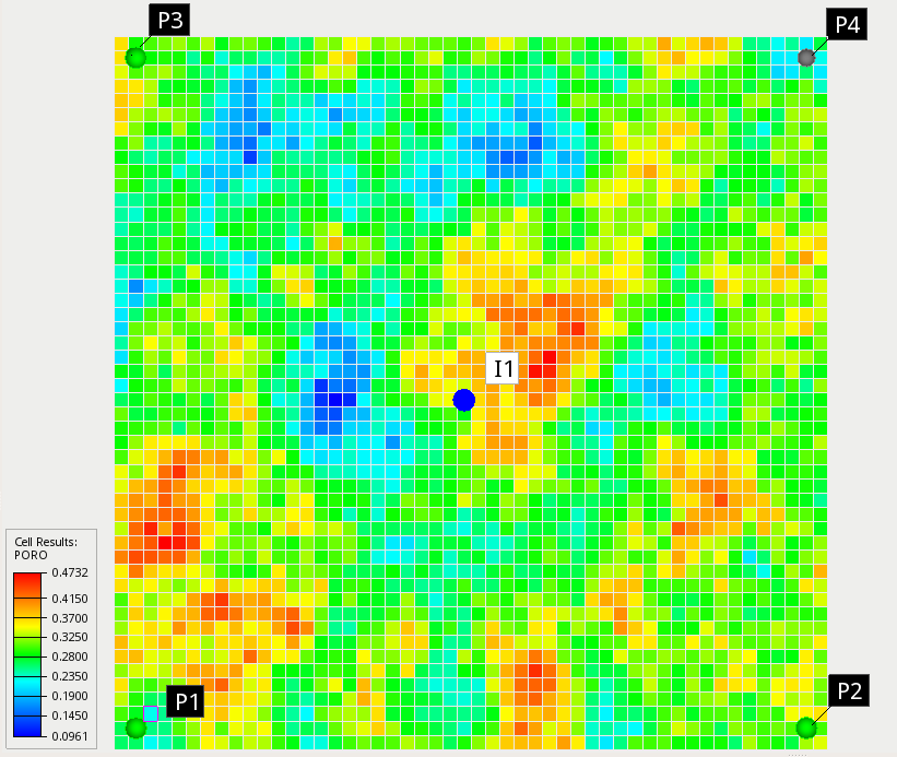
Figure 2: Porosity distribution of the five-spot field and placement of the injection and production wells.

On average, the reservoir has approximately $30$% porosity with a heterogeneous permeability distribution. The initial reservoir pressure is $200$ bar. The initial average oil and water saturations are $0.6546$ and $0.3454$, respectively. The original oil in place is $4.983\cdot 10^{6}$ sm³. Fluid properties are similar to those of a light oil reservoir. The viscosity for saturated oil at varying bubble point pressure lies between $0.1$ cP and $0.56$ cP, and the viscosity of water is $0.01$ cP. The densities of oil and water are taken as $732$ kg/m³ and $1000$ kg/m³, respectively. In this setting, it is easy to see that the displacement is unfavorable since the oil-water mobility ratio $\lambda$ is such that $10\leq\lambda\leq 56$. The reservoir rock parameters utilized for the polymer flooding simulation in this problem are given by Table 1.

Parameter	Value	Unit
Dead pore space for polymer solution	$0.1800$	$-$
Maximum polymer adsorption value	$7.5\cdot 10^{-4}$	kg/kg
Residual resistance factor of polymer solution	$2.5$	$-$
Reservoir rock density	$1980$	$\text{kg/rm}^{3}$
Polymer mixing parameters	$0.65$	$-$

Table 1: Reservoir model parameters used in the polymer flooding simulations.

In this example, the injection well is controlled by two independent control variables, namely the water injection rate and the polymer concentration at each control time step. The lower and upper bounds for the water injection rate are set to $0$ sm³/day and $2000$ sm³/day respectively, while the lower and upper bounds for the polymer concentration are set to $0$ kg/sm³ and $2.5$ kg/sm³. Hence, the polymer injection rate ranges from $0$ to $5000$ kg/day. Each production well is controlled by a reservoir fluid production rate target with a lower limit of $0$ sm³/day and an upper limit of $500$ sm³/day. Bottom hole pressure limits are imposed on the wells, namely a maximum of $500$ bar for the injector and a minimum of $150$ bar for each producer. The production period for the reservoir is set to $50$ months, and the control time step is taken as $5$ months. Therefore, there are $N_{u}=(2+4)\times 10=60$ control variables in total to solve for in (3). For the objective function (3a), we used the economic parameters listed in Table 2.

Parameter	Value	Unit
Oil price $r_{\text{OP}}$	$500$	USD/sm3
Price of gas production $r_{\text{GP}}$	$0.15$	USD/sm3
Cost of polymer injection $r_{\text{PI}}$	2.5	USD/kg
Cost of polymer production $r_{\text{PP}}$	0.5	USD/kg
Cost of water injection or production $r_{\text{WI}}$, $r_{\text{WP}}$	$30$	USD/sm3
Annual discount rate $d_{\tau}$	$0.1$	$-$

Table 2: Economic parameters used in the numerical experiments.

Using the two different surrogate models for the objective function (3a) constructed by means of neural networks, namely DNN_s and DNN_v as explained in Section 5, the optimization problem (3) is solved using the Adaptive-ML-EnOpt algorithm. In this case, the Adaptive-ML-EnOpt algorithm for (3) using DNN_s and DNN_v to approximate the objective function $J$ from (3a) is denoted by AML-EnOpt_s and AML-EnOpt_v, respectively. The EnOpt parameters for both, the FOM-EnOpt and the two variants of the Adaptive-ML-EnOpt method, are presented in Table 3. We remark that the tolerances $\varepsilon$, $\varepsilon_{i}$, and $\varepsilon_{o}$ are applied to the scaled quantities, i.e., the output quantities, for which the respective stopping criteria in Algorithms 1 and 5 are checked, have already been scaled as described in Section 6.1.

Parameter	Value
Initial step size $\beta_{0}$	$0.3$
Step size contraction $r$	$0.5$
Maximum step size trials $\nu^{*}$	$10$
Initial control-type variance $\sigma_{j}$	$0.001$
Constant correlation factor $\rho$	$0.9$
Perturbation size $N$	$100$
Tolerances FOM-EnOpt $\varepsilon$ Adaptive-ML-EnOpt inner iteration $\varepsilon_{i}$ Adaptive-ML-EnOpt outer iteration $\varepsilon_{o}$	$10^{-6}$ $10^{-6}$ $10^{-2}$

Table 3: Parameters used in the FOM-EnOpt and Adaptive-ML-EnOpt algorithms.

We compare the Adaptive-ML-EnOpt results with those of the FOM-EnOpt algorithm for two different initial guesses $\textbf{u}_{0}^{1}\in\mathcal{D}_{\text{ad}}$ and $\textbf{u}_{0}^{2}\in\mathcal{D}_{\text{ad}}$. The initial solution $\textbf{u}_{0}^{1}$ includes $700$ sm³/day for the water injection rate at the injection well, $150$ sm³/day for the reservoir fluid production rate at each production well, and $0.5$ kg/sm³ for the polymer concentration (equivalently $350$ kg/day for polymer injection rate) at the injection well over the simulation period. Similarly, $\textbf{u}_{0}^{2}$ includes $600$ sm³/day for the water injection rate, $100$ sm³/day for the reservoir fluid production rate, and $0.5$ kg/sm³ for the polymer concentration.

Figure 3: Comparison of the NPV values obtained during the outer iterations of the FOM-EnOpt, AML-EnOpt_s, and AML-EnOpt_v procedures for two different initial guesses $\textbf{u}_{0}^{1}\in\mathcal{D}_{\text{ad}}$ and $\textbf{u}_{0}^{2}\in\mathcal{D}_{\text{ad}}$. For each Adaptive-ML-EnOpt procedure, the corresponding FOM value $J(\textbf{u}_{k})$ at the current iterate $\textbf{u}_{k}$ of the respective Adaptive-ML-EnOpt method is indicated as well.

Figure 3 compares the values of the objective function during the outer iterations of the FOM-EnOpt, AML-EnOpt_s, and AML-EnOpt_v strategies using the initial solutions $\textbf{u}_{0}^{1}$ and $\textbf{u}_{0}^{2}$. Furthermore, the value $J(\textbf{u}_{k})$ at the outer iterate $\textbf{u}_{k}$ (denoted by “FOM value”) for the respective Adaptive-ML-EnOpt method is depicted.

Since the Adaptive-ML-EnOpt algorithms only use an approximate surrogate model $J_{\text{ML}}^{k}$, the values of $J$ and $J_{\text{ML}}^{k}$ are not necessarily the same for the control $\textbf{u}_{k}$. This behavior is especially apparent in Figure 3(b), where the AML-EnOpt_v algorithm is examined for the initial guess $\textbf{u}_{0}^{1}$. Here, after the first outer iteration, the values $J(\textbf{u}_{1})$ and $J_{\text{ML}}^{0}(\textbf{u}_{1})$ differ from each other by a significant amount. A possible reason is that the surrogate model $J_{\text{ML}}^{0}$ does not extrapolate well to the region where the first (inner) Adaptive-ML-EnOpt iteration converged to. This further indicates that the found iterate $\textbf{u}_{1}$ is far from the initial solution $\textbf{u}_{0}$, where the initial model $J_{\text{ML}}^{0}$ was trained. However, since the Adaptive-ML-EnOpt algorithm uses evaluations of $J$ in the stopping criterion, the Adaptive-ML-EnOpt does not terminate but continues by training a new surrogate model using training data sampled normally around $\textbf{u}_{1}$. Hence, the new surrogate $J_{\text{ML}}^{1}$ tries to approximate the objective function $J$ well around $\textbf{u}_{1}$. In each plot, we see that in the last two outer iterations of the respective Adaptive-ML-EnOpt procedure, the FOM value and the Adaptive-ML-EnOpt value agree to minimal deviations. This suggests that the surrogate model approximates the full objective function well in the region of the (local) optimum found by the Adaptive-ML-EnOpt method.

More so, in Figure 3, it is seen that both, the AML-EnOpt_s and the AML-EnOpt_v algorithm, require considerably less (costly) outer iterations than the FOM-EnOpt method. This leads to an improvement in the run time of the method, which is detailed in Table 4. Besides the faster convergence of the method, we also remark that the Adaptive-ML-EnOpt algorithms find local optima with larger objective function values than the FOM-EnOpt algorithm. However, since the objective function $J$ is multi-modal, this is not guaranteed.

We emphasize that each outer iteration of the Adaptive-ML-EnOpt algorithm includes many inner iterations (see also Tables 4 and 5), which leads to the large jumps in the objective function values between consecutive outer iterations, as present in Figure 3.

Further comparisons in terms of function values, numbers of inner and outer iterations, numbers of evaluations of the FOM function $J$ and surrogate approximations $J_{\text{ML}}^{k}$, total run time, and speedup are presented in Tables 4 and 5.

With the different initial guesses $\textbf{u}_{0}^{1}$ and $\textbf{u}_{0}^{2},$ we found that the number of outer iterations required by the FOM-EnOpt algorithm significantly differs. However, the Adaptive-ML-EnOpt methods require only $4$ and $5$ outer iterations. This reduced number of outer iterations leads to a remarkable speedup in the overall computation time $T_{\text{total}}$ and is particularly reflected in the reduced number of FOM evaluations, i.e., evaluations of the objective function $J$, which require costly polymer flooding simulations. Although each outer iteration consists of multiple inner iterations using the surrogate $J_{\text{ML}}^{k}$, it does not contribute substantially to the overall run time because evaluating the surrogate $J_{\text{ML}}^{k}$ is very cheap.

Method	FOM value	Surrogate value	Outer it.	Inner it.	FOM eval.	Surrogate eval.	$T_{\text{total}}$ (min)	Speedup
FOM-EnOpt	$6.400\cdot 10^{8}$	$-$	28	$-$	$2839$	$-$	$54.86$	$-$
AML-EnOpts	$7.013\cdot 10^{8}$	$6.968\cdot 10^{8}$	$4$	$233$	$407$	$12315$	$8.87$	$6.18$
AML-EnOptv	$7.185\cdot 10^{8}$	$7.168\cdot 10^{8}$	$5$	$312$	$509$	$14101$	$14.10$	$3.89$

Table 4: Comparisons of the results from the different solution strategies FOM-EnOpt, AML-EnOpt_s, and AML-EnOpt_v using the initial guess $\textbf{u}_{0}^{1}$ and $N_{1}=N_{2}=35$ neurons in each hidden layer and $15$ restarts for the neural network training.

Method	FOM value	Surrogate value	Outer it.	Inner it.	FOM eval.	Surrogate eval.	$T_{\text{total}}$ (min)	Speedup
FOM-EnOpt	$4.895\cdot 10^{8}$	$-$	92	$-$	$9310$	$-$	$135.77$	$-$
AML-EnOpts	$5.754\cdot 10^{8}$	$5.816\cdot 10^{8}$	$4$	$111$	$407$	$10837$	$9.85$	$13.78$
AML-EnOptv	$5.942\cdot 10^{8}$	$5.908\cdot 10^{8}$	$4$	$117$	$407$	$10033$	$11.05$	$12.29$

Table 5: Comparisons of the results from the different solution strategies FOM-EnOpt, AML-EnOpt_s, and AML-EnOpt_v using the initial guess $\textbf{u}_{0}^{2}$ and $N_{1}=N_{2}=25$ neurons in each hidden layer and $35$ restarts for the neural network training.

For the initial solution $\textbf{u}_{0}^{1}$, the optimizers obtained from the three solution strategies are depicted in Figure 4. Further, the initial guess $\textbf{u}_{0}^{1}$ is shown as a reference.

The control variables obtained by the AML-EnOpt_s and the AML-EnOpt_v algorithm are close to those of the FOM-EnOpt method, except for production well 3 (see Figure 4(c)) and the water injection rate (see Figure 4(e)). For each control variable, the values obtained via the AML-EnOpt_s and AML-EnOpt_v procedures are close to each other. Together with the FOM values of AML-EnOpt_s and AML-EnOpt_v presented in Table 4 and the evolution of the FOM values for the two methods shown in Figure 3(a)-(b), this suggests that the AML-EnOpt_s and the AML-EnOpt_v methods traverse almost the same path in the control space $\mathcal{D}_{\text{ad}}$ and find local optima close to each other.

Figure 4: Comparison of the optimal solutions obtained via the FOM-EnOpt, AML-EnOpt_s, and AML-EnOpt_v algorithms using the initial guess $\textbf{u}_{0}^{1}$, which is depicted as the reference solution.

Figure 5(a) depicts a comparison of the total field oil production for the optimal solutions (in Figure 4) of the three solution methods. The total field oil production by FOM-EnOpt, AML-EnOpt_s, and AML-EnOpt_v are $1.343\cdot 10^{6}$, $1.425\cdot 10^{6}$, and $1.554\cdot 10^{6}$ (in sm³), respectively. The solution obtained by AML-EnOpt_v attains the highest oil production in total, followed by the AML-EnOpt_s. The total back-produced water and polymer from operating the five-spot field with the different optimal solutions are presented in Figure 5(b) and Figure 5(c), respectively. Here, we found that the AML-EnOpt_s and AML-EnOpt_v solutions are more economical and environmentally friendly than the one provided by using the FOM-EnOpt method.

Figure 5: Comparison of the production data obtained from the different solution strategies FOM-EnOpt, AML-EnOpt_s, and AML-EnOpt_v using the initial guess $\textbf{u}_{0}^{1}$.

To further investigate the effects of different neural network architectures on the resulting NPV values, Figure 6 depicts the NPV values obtained by the Adaptive-ML-EnOpt algorithm when using different numbers of neurons in the hidden layers of the surrogate models DNN_s and DNN_v.

We observe that the AML-EnOpt_v method results are very similar, which suggests that the DNN_v-approach is more robust and leads to similar optimal solutions independent of the neural network structure. In the case of the AML-EnOpt_s algorithm, different numbers of neurons lead to results with a larger variation. In particular, the number of outer iterations performed is different. Hence, the architecture of the underlying network seems to have a significant effect on the performance of the resulting AML-EnOpt_s algorithm.

Figure 6: Comparison of the Adaptive-ML-EnOpt procedures AML-EnOpt_s and AML-EnOpt_v for different numbers of neurons in the hidden layers with fixed initial guess $\textbf{u}_{0}^{1}$.

The maximum, minimum, and average training and validation losses that occurred in the AML-EnOpt_s and AML-EnOpt_v algorithm for the initial guess $\textbf{u}_{0}^{1}$ are presented in Table 6. The table shows the respective MSE losses for different numbers of neurons in the hidden layers.

The results in Table 6 do not suggest a significant influence of the number of neurons on the training and validation results. Further, the scalar- and vector-valued cases, DNN_s and DNN_v respectively, perform similarly in overall training and validation losses. However, we emphasize that, in the DNN_v case, the MSE loss cannot be related directly to the difference in the output function. Instead, one has to take into account that the outputs of DNN_v are summed up to obtain the surrogate $J_{\text{ML}}^{k}$, while the MSE loss is measured on the vector-valued outputs of the neural network.

Altogether, the numerical experiments with different numbers of neurons suggest that already small DNNs with only $20$ neurons in each of the hidden layers yield appropriate results. In this specific application, we do not benefit from increasing the complexity of the neural network. We have seen the same behavior when using more than two hidden layers.

Method	Neurons $N_{1}=N_{2}$	Outer iter.	Training loss			Validation loss
			Max.	Min.	Avg.	Max.	Min.	Avg.
DNNs	$20$	$4$	$1.2\cdot 10^{-4}$	$1.3\cdot 10^{-6}$	$5.3\cdot 10^{-5}$	$5.4\cdot 10^{-3}$	$6.7\cdot 10^{-5}$	$2.3\cdot 10^{-3}$
DNNs	$25$	$2$	$6.0\cdot 10^{-4}$	$1.3\cdot 10^{-6}$	$3.0\cdot 10^{-4}$	$2.3\cdot 10^{-3}$	$2.1\cdot 10^{-3}$	$2.2\cdot 10^{-3}$
DNNs	$30$	$7$	$7.9\cdot 10^{-4}$	$8.5\cdot 10^{-7}$	$1.7\cdot 10^{-4}$	$6.6\cdot 10^{-3}$	$1.7\cdot 10^{-3}$	$3.6\cdot 10^{-3}$
DNNs	$35$	$4$	$1.8\cdot 10^{-4}$	$6.1\cdot 10^{-6}$	$8.2\cdot 10^{-5}$	$5.5\cdot 10^{-3}$	$3.7\cdot 10^{-4}$	$2.7\cdot 10^{-3}$
DNNv	$20$	$5$	$1.8\cdot 10^{-3}$	$2.1\cdot 10^{-5}$	$5.2\cdot 10^{-4}$	$6.9\cdot 10^{-3}$	$1.2\cdot 10^{-3}$	$4.2\cdot 10^{-3}$
DNNv	$25$	$6$	$9.9\cdot 10^{-4}$	$1.5\cdot 10^{-5}$	$4.1\cdot 10^{-4}$	$6.4\cdot 10^{-3}$	$9.4\cdot 10^{-4}$	$3.6\cdot 10^{-3}$
DNNv	$30$	$5$	$9.0\cdot 10^{-4}$	$9.9\cdot 10^{-6}$	$4.0\cdot 10^{-4}$	$1.0\cdot 10^{-2}$	$5.2\cdot 10^{-4}$	$4.3\cdot 10^{-3}$
DNNv	$35$	$5$	$6.0\cdot 10^{-4}$	$1.1\cdot 10^{-6}$	$2.2\cdot 10^{-4}$	$8.8\cdot 10^{-3}$	$4.6\cdot 10^{-4}$	$4.3\cdot 10^{-3}$

Table 6: Maximum, minimum, and average MSE loss in the AML-EnOpt_s and AML-EnOpt_v algorithm with different numbers of neurons in the hidden layers of the neural networks DNN_s and DNN_v for fixed initial guess $\textbf{u}_{0}^{1}$. The number of hidden layers is fixed to two.

7 Conclusion and future work

In this contribution, we presented a new algorithm to speed up PDE-constrained optimization problems occurring in the context of enhanced oil recovery. The algorithm is based on adaptively constructed surrogate models that make use of deep neural networks for approximating the objective functional. In each outer iteration of the algorithm, a new surrogate model is trained with data consisting of full-order function evaluations around the current control point. Afterwards, an ensemble-based optimization algorithm is applied to the surrogate to obtain a candidate for the next iteration. We perform full order model evaluations to validate whether the resulting controls correspond to a local optimum of the true objective functional. These function evaluations also serve as training data for constructing the next surrogate.

Our numerical results confirm that the described algorithm can accelerate the solution of the enhanced oil recovery optimization problem. At the same time, in our numerical experiments, the procedure produces controls with even larger objective function values than those obtained using only costly full-order model evaluations. However, we should emphasize that such an improvement in the objective function value is not guaranteed and, in our case, results from the multi-modal structure of the objective functional.

The investigated five-spot benchmark problem served as a proof of concept for our Adaptive-ML-EnOpt algorithm, where FOM evaluations were relatively quickly accessible, and the input dimension was of moderate size. Future research is thus devoted to more involved numerical experiments with more significant complexity.

As indicated in the optimization problem description, we focused on a scenario with fixed geological properties. However, in practical applications, these geological parameters are usually unknown and typically treated by ensemble-based methods, where the ensemble is to be understood not only with respect to perturbations of the controls for approximating the gradient but also with respect to different samples of geological properties. One of the central future research perspectives is incorporating such geological uncertainty in our algorithm. The main challenge is the high dimension of the space of possible geological parameters. Naively using these parameters as additional inputs for the neural network is thus not feasible. Future research might consider reducing the dimension of the space of geological parameters by incorporating additional information on the distribution of such parameters and passing the reduced variables to the neural networks.

Furthermore, replacing neural networks as surrogate models for the objective function, for instance, by polynomial approximations obtained via linear regression or by different machine learning approaches, such as kernel methods [20], could be investigated further. The Adaptive-ML-EnOpt algorithm is formulated in such a way that replacing the surrogate model and its training is readily possible. Any approximation of the objective function built from evaluations of the true objective function is feasible and can directly be used in the algorithm. In addition, the inner iterations are not restricted to the EnOpt procedure but can also be performed using different optimization routines. However, we should emphasize that in the current formulation, no information on the exact gradient, neither of the true objective functional nor the surrogate model, is required. This might change when employing different optimization routines. Moreover, the presented approach is not restricted to the NPV objective functional in enhanced oil recovery but can be generalized to any scalar-valued quantity of interest. The algorithm might be of particular relevance in cases where no direct access to the underlying PDE solutions is possible, and no error estimation for the surrogate model is available.

References

- [1] A. Abidin, T. Puspasari, and W. Nugroho. Polymers for enhanced oil recovery technology. Procedia Chemistry, 4:11–16, 2012.
- [2] M. A. Ahmadi. Developing a robust surrogate model of chemical flooding based on the artificial neural network for enhanced oil recovery implications. Mathematical Problems in Engineering, 2015:9, 2015.
- [3] S. Banholzer, T. Keil, L. Mechelli, M. Ohlberger, F. Schindler, and S. Volkwein. An adaptive projected newton non-conforming dual approach for trust-region reduced basis approximation of pde-constrained parameter optimization, 2020. arXiv-eprint:2012.11653.
- [4] K. Bao, K.-A. Lie, O. Møyner, and M. Liu. Fully implicit simulation of polymer flooding with mrst. Computational Geosciences, 21(5):1219–1244, 2017.
- [5] D. Baxendale, A. F. Rasmussen, A. B. Rustad, T. Skille, and T. H. Sandve. Opm flow documentation manual manual. Open Porous Media Initiative, 2021.
- [6] P. Benner, M. Ohlberger, A. Patera, G. Rozza, and K. Urban, editors. Model reduction of parametrized systems, volume 17 of MS&A. Modeling, Simulation and Applications. Springer, Cham, 2017. Selected papers from the 3rd MoRePaS Conference held at the International School for Advanced Studies (SISSA), Trieste, October 13–16, 2015.
- [7] L. Bottou, F. E. Curtis, and J. Nocedal. Optimization methods for large-scale machine learning. SIAM Rev., 60(2):223–311, 2018.
- [8] Y. Chen, D. S. Oliver, and D. Zhang. Efficient ensemble-based closed-loop production optimization. SPE Journal, 14(04):634–645, 2009.
- [9] Z. Chen. Reservoir simulation: mathematical techniques in oil recovery. SIAM, 2007.
- [10] Y. Cheraghi, S. Kord, and V. Mashayekhizadeh. Application of machine learning techniques for selecting the most suitable enhanced oil recovery method; challenges and opportunities. Journal of Petroleum Science and Engineering, 205:108761, 2021.
- [11] D. Elbrächter, P. Grohs, A. Jentzen, and C. Schwab. Dnn expression rate analysis of high-dimensional pdes: Application to option pricing. Constructive Approximation, 2021.
- [12] R. Fonseca, S. Kahrobaei, L. Van Gastel, O. Leeuwenburgh, and J. Jansen. Quantification of the impact of ensemble size on the quality of an ensemble gradient using principles of hypothesis testing. In SPE Reservoir Simulation Symposium. OnePetro, 2015.
- [13] R. R.-M. Fonseca, B. Chen, J. D. Jansen, and A. Reynolds. A stochastic simplex approximate gradient (stosag) for optimization under uncertainty. International Journal for Numerical Methods in Engineering, 109(13):1756–1776, 2017.
- [14] P. Gavrilenko, B. Haasdonk, O. Iliev, M. Ohlberger, F. Schindler, P. Toktaliev, T. Wenzel, and M. Youssef. A full order, reduced order and machine learning model pipeline for efficient prediction of reactive flows. 2021. arXiv-eprint:2104.02800.
- [15] A. Golzari, M. Haghighat Sefat, and S. Jamshidi. Development of an adaptive surrogate model for production optimization. Journal of Petroleum Science and Engineering, 133:677–688, 2015.
- [16] E. J. Gudiña, E. C. Fernandes, A. I. Rodrigues, J. A. Teixeira, and L. R. Rodrigues. Biosurfactant production by bacillus subtilis using corn steep liquor as culture medium. Frontiers in microbiology, 6:59, 2015.
- [17] B. Haasdonk, M. Ohlberger, and F. Schindler. An adaptive model hierarchy for data-augmented training of kernel models for reactive flow. 2021. arXiv-eprint:2110.12388.
- [18] T. Hastie, R. Tibshirani, and J. Friedman. The Elements of Statistical Learning. 10.1007/978-0-387-84858-7, 2009.
- [19] K. He, X. Zhang, S. Ren, and J. Sun. Delving deep into rectifiers: Surpassing human-level performance on imagenet classification. In 2015 IEEE International Conference on Computer Vision (ICCV), pages 1026–1034, 2015.
- [20] T. Hofmann, B. Schölkopf, and A. J. Smola. Kernel methods in machine learning. The Annals of Statistics, 36(3):1171 – 1220, 2008.
- [21] J. Holmes. Enhancements to the strongly coupled, fully implicit well model: wellbore crossflow modeling and collective well control. In SPE Reservoir Simulation Symposium. OnePetro, 1983.
- [22] J. Holmes, T. Barkve, and O. Lund. Application of a multisegment well model to simulate flow in advanced wells. In European petroleum conference. OnePetro, 1998.
- [23] T. Keil, L. Mechelli, M. Ohlberger, F. Schindler, and S. Volkwein. A non-conforming dual approach for adaptive trust-region reduced basis approximation of PDE-constrained parameter optimization. ESAIM Math. Model. Numer. Anal., 55(3):1239–1269, 2021.
- [24] Y. LeCun, Y. Bengio, and G. Hinton. Deep learning. Nature, 521:436–44, 2015.
- [25] J.-Y. Lee, H.-J. Shin, and J.-S. Lim. Selection and evaluation of enhanced oil recovery method using artificial neural network. Geosystem Engineering, 14:157 – 164, 2011.
- [26] D. C. Liu and J. Nocedal. On the limited memory BFGS method for large scale optimization. Mathematical Programming, 45:503–528, 1989.
- [27] R. Lu and A. Reynolds. Joint optimization of well locations, types, drilling order, and controls given a set of potential drilling paths. SPE Journal, 25(03):1285–1306, 2020.
- [28] K. O. Lye, S. Mishra, D. Ray, and P. Chandrashekar. Iterative surrogate model optimization (ismo): An active learning algorithm for pde constrained optimization with deep neural networks. Computer Methods in Applied Mechanics and Engineering, 374:113575, 2021.
- [29] R. Milk, S. Rave, and F. Schindler. pyMOR – generic algorithms and interfaces for model order reduction. SIAM J. Sci. Comput., 38(5):S194–S216, jan 2016.
- [30] D. C. Montgomery, C. L. Jennings, and M. Kulahci. Introduction to time series analysis and forecasting. John Wiley & Sons, 2015.
- [31] J. Nocedal and S. Wright. Numerical optimization. Springer Science & Business Media, 2006.
- [32] M. B. Oguntola and R. J. Lorentzen. On the robust value quantification of polymer eor injection strategies for better decision making. In ECMOR XVII, volume 2020, pages 1–25. European Association of Geoscientists & Engineers, 2020.
- [33] M. B. Oguntola and R. J. Lorentzen. Ensemble-based constrained optimization using an exterior penalty method. Journal of Petroleum Science and Engineering, 207:109165, 2021.
- [34] S. Pancholi, G. S. Negi, J. R. Agarwal, A. Bera, and M. Shah. Experimental and simulation studies for optimization of water–alternating-gas (co2) flooding for enhanced oil recovery. Petroleum Research, 5(3):227–234, 2020.
- [35] A. Paszke, S. Gross, F. Massa, A. Lerer, J. Bradbury, G. Chanan, T. Killeen, Z. Lin, N. Gimelshein, L. Antiga, A. Desmaison, A. Kopf, E. Yang, Z. DeVito, M. Raison, A. Tejani, S. Chilamkurthy, B. Steiner, L. Fang, J. Bai, and S. Chintala. Pytorch: An imperative style, high-performance deep learning library. In H. Wallach, H. Larochelle, A. Beygelzimer, F. d’ Alché-Buc, E. Fox, and R. Garnett, editors, Advances in Neural Information Processing Systems 32, pages 8024–8035. Curran Associates, Inc., 2019.
- [36] P. Petersen and F. Voigtlaender. Optimal approximation of piecewise smooth functions using deep relu neural networks. Neural Networks, 108:296 – 330, 2018.
- [37] L. Prechelt. Early stopping - but when? In Neural Networks: Tricks of the Trade, volume 1524 of LNCS, chapter 2, pages 55–69. Springer-Verlag, 1997.
- [38] A. F. Rasmussen, T. H. Sandve, K. Bao, A. Lauser, J. Hove, B. Skaflestad, R. Klöfkorn, M. Blatt, A. B. Rustad, O. Sævareid, et al. The open porous media flow reservoir simulator. Computers & Mathematics with Applications, 81:159–185, 2021.
- [39] D. E. Rumelhart, G. E. Hintont, and R. J. Williams. Learning representations by back-propagating errors. Nature, 323(6088):533–536, 1986.
- [40] H. Saberi, E. Esmaeilnezhad, and H. J. Choi. Artificial neural network to forecast enhanced oil recovery using hydrolyzed polyacrylamide in sandstone and carbonate reservoirs. Polymers, 13(16), 2021.
- [41] P. Sarma, L. J. Durlofsky, K. Aziz, and W. H. Chen. Efficient real-time reservoir management using adjoint-based optimal control and model updating. Computational Geosciences, 10(1):3–36, 2006.
- [42] A. S. Stordal, S. P. Szklarz, and O. Leeuwenburgh. A theoretical look at ensemble-based optimization in reservoir management. Mathematical Geosciences, 48(4):399–417, 2016.
- [43] S. L. Van and B. H. Chon. Well-pattern investigation and selection by surfactant-polymer flooding performance in heterogeneous reservoir consisting of interbedded low-permeability layer. Korean Journal of Chemical Engineering, 33(12):3456–3464, 2016.
- [44] D. Wang, R. S. Seright, Z. Shao, J. Wang, et al. Key aspects of project design for polymer flooding at the daqing oilfield. SPE Reservoir Evaluation & Engineering, 11(06):1–117, 2008.
- [45] S. Wang, M. A. Bhouri, and P. Perdikaris. Fast pde-constrained optimization via self-supervised operator learning, 2021. arXiv-eprint:2110.13297.
- [46] P. Wolfe. Convergence conditions for ascent methods. SIAM Review, 11(2):226–235, 1969.
- [47] P. Wolfe. Convergence conditions for ascent methods. ii: Some corrections. SIAM Review, 13(2):185–188, 1971.
- [48] L. Xu, H. Zhao, Y. Li, L. Cao, X. Xie, X. Zhang, and Y. Li. Production optimization of polymer flooding using improved monte carlo gradient approximation algorithm with constraints. Journal of Circuits, Systems and Computers, 27(11):1850167, 2018.
- [49] D. Yarotsky. Error bounds for approximations with deep ReLU networks. Neural Networks, 94:103 – 114, 2017.
- [50] M. J. Zahr and C. Farhat. Progressive construction of a parametric reduced-order model for PDE-constrained optimization. Int. J. Numer. Meth. Engng, 102:1111–1135, 2015.
- [51] Y. Zhang, R. Lu, F. Forouzanfar, and A. C. Reynolds. Well placement and control optimization for wag/sag processes using ensemble-based method. Computers & Chemical Engineering, 101:193–209, 2017.
- [52] K. Zhou, J. Hou, X. Zhang, Q. Du, X. Kang, and S. Jiang. Optimal control of polymer flooding based on simultaneous perturbation stochastic approximation method guided by finite difference gradient. Computers & chemical engineering, 55:40–49, 2013.