Translational Lung Imaging Analysis Through Disentangled Representations

Abstract

The development of new treatments often requires clinical trials with translational animal models using (pre)-clinical imaging to characterize inter-species pathological processes. Deep Learning (DL) models are commonly used to automate retrieving relevant information from the images. Nevertheless, they typically suffer from low generability and explainability as a product of their entangled design, resulting in a specific DL model per animal model. Consequently, it is not possible to take advantage of the high capacity of DL to discover statistical relationships from inter-species images.
To alleviate this problem, in this work, we present a model capable of extracting disentangled information from images of different animal models and the mechanisms that generate the images. Our method is located at the intersection between deep generative models, disentanglement and causal representation learning. It is optimized from images of pathological lung infected by Tuberculosis and is able: a) from an input slice, infer its position in a volume, the animal model to which it belongs, the damage present and even more, generate a mask covering the whole lung (similar overlap measures to the nnU-Net), b) generate realistic lung images by setting the above variables and c) generate counterfactual images, namely, healthy versions of a damaged input slice.

1 Introduction

The longitudinal characterization of animal models is crucial during (pre-)clinical drug trials. To characterize disease progression meaningfully, we need to have the capacity to extract comparable biomarkers in similar phases of the disease progression. Besides, we need to prove the existence of similar pathophysiological mechanisms modulating common causal factors that give rise to the variability of trial outcomes.
In this context, medical imaging techniques enable the extraction of indicators (imaging biomarkers) from in vivo studies [Willmann et al.(2008)Willmann, van Bruggen, Dinkelborg, and Gambhir]. For example, the number of Mycobacterium tuberculosis (Mtb.) colonies present in a subject can be inferred from the damaged lung volume in an image of a human, primate, or mouse [Yang et al.(2021)Yang, Wang, Wen, Weiner, and Via].
The images contain meaningful information to interpret the mentioned physiological process. However, their manual analysis is tedious, and automation is advantageous to process the vast amount of data produced during the trials. Thus, developing Artificial Intelligence (AI) systems that can not only automate the extraction of particular markers for each animal model (e.g., the damaged lung volume) but are also capable of inferring the common agents of such particular indicators (e.g., bacterial burden) is essential.

Although AI, especially Deep Learning (DL), has eased the process [Zhou et al.(2021)Zhou, Greenspan, Davatzikos, Duncan, van Ginneken, Madabhushi, Prince, Rueckert, and Summers, Hinton(2018)], some design premises has lessened its inference capabilities. In particular, DL models excel at extracting the statistical dependence between input-output pairs, i.e.,$(x_{i},y_{i})\in\mathcal{X,Y}$, from assumed independent and identically distributed (i.i.d.) observational data [Peters et al.(2017)Peters, Janzing, and Schölkopf].

Such success has leaned the model designs towards an insufficient representation learning strategy [Bengio et al.(2013)Bengio, Courville, and Vincent]. Namely, discovering statistical dependence between specific data pair samples is prioritized rather than understanding the physical model generating the whole data population (e.g., physiological mechanisms).

Since the i.i.d. assumption is fragile, well-known distribution shifts [Castro et al.(2020)Castro, Walker, and Glocker] between data employed at training, validation and test phases, and real-world data are usual. Under this scenario, the models tend to learn correlated representations that only hold for specific environments or domains, namely spurious correlations [Arjovsky et al.(2020)Arjovsky, Bottou, Gulrajani, and Lopez-Paz]. Since (as a mantra) correlation does not imply causation, such flaws cause ruinous effects [DeGrave et al.(2021)DeGrave, Janizek, and Lee, Roberts et al.(2021)Roberts, Driggs, Thorpe, Gilbey, Yeung, Ursprung, Aviles-Rivero, Etmann, McCague, Beer, Weir-McCall, Teng, Gkrania-Klotsas, Ruggiero, Korhonen, Jefferson, Ako, Langs, Gozaliasl, Yang, Prosch, Preller, Stanczuk, Tang, Hofmanninger, Babar, Sánchez, Thillai, Gonzalez, Teare, Zhu, Patel, Cafolla, Azadbakht, Jacob, Lowe, Zhang, Bradley, Wassin, Holzer, Ji, Ortet, Ai, Walton, Lio, Stranks, Shadbahr, Lin, Zha, Niu, Rudd, Sala, and Schönlieb] for generalisation, transferability and explainability purposes [Scholkopf et al.(2021)Scholkopf, Locatello, Bauer, Ke, Kalchbrenner, Goyal, and Bengio].

More formally, naive DL models maximize a joint distribution, $p(X,Y)$ or $p(X)$ (self-supervision), characterized by an entangled representation of the input. Namely, if $X$ and $Y$ correlate during training without necessarily deriving from a causal representation ($X\rightarrow Y$), $p(X,Y)$ can adopt numerous factorization forms that are domain-specific [Goyal and Bengio(2021)]. Thus, forcing to implement independent models even for related domains (in our case, lung CT images of TB animal models). Such models are put in common through posthoc analysis, losing possible data synergies.

In general, learning strategies mitigate this issue by shrinking the $p(X,Y)$ solutions space. To this aim, models are enriched injecting inductive biases (e.g., CNNs assume spatial correlation [Dumoulin and Visin(2018)]), to facilitate the discovery of more meaningful and disentangled representations [Liu et al.(2021)Liu, Sanchez, Thermos, O’Neil, and Tsaftaris]. These strategies resemble human cognition. Since, humans arrange the proper biases to extract a limited number of relevant factors transferable among different environments [Pearl(2011)].

AI systems design can follow a similar causal perspective. Namely, specific biases can be introduced to shrink the solution space. Thus, in this work, we consider the bias: a) the strongly hierarchical nature of the human visual system and b) the data generation process. Such an approach intends to mimic the radiologists’ tasks, who take into account specific patient factors (i.e., clinical history, sex, age) beyond the image per se. This approach yields more effective disentangled representations of the input [Scholkopf et al.(2021)Scholkopf, Locatello, Bauer, Ke, Kalchbrenner, Goyal, and Bengio].

In particular, we intend to identify the unique mechanisms that govern the generation of translational imaging of lung Computed Tomography (CT) images and their corresponding segmentation masks (fig:DAG). We employ three different animal models (mouse, primate and human) infected by Mtb. [Pai et al.(2016)Pai, Behr, Dowdy, Dheda, Divangahi, Boehme, Ginsberg, Swaminathan, Spigelman, Getahun, Menzies, and Raviglione]. From a simplified radiological point of view, mammals’ lungs share texture and shape features. We model these shared attributes as an effect of the same causative factors, e.g., bacterial load (see Appendix A).
To prove the benefits of our strategy, we show how after optimizing the model employing a small limited number of volumes, our design can:

• Produce a very accurate reconstruction of the input images and generate suitable segmentation masks (fig:lungs_seg, tbl:optimiza_results).

• Generate new realistic images of the three different animal models controlling the lung damage on each, which implies the proper characterization of the disentangled variables (fig:generated).

• Generate counterfactual images of damaged lungs [Schutte et al.(2021)Schutte, Moindrot, Hérent, Schiratti, and Jégou, Cohen et al.(2021)Cohen, Brooks, En, Zucker, Pareek, Lungren, and Chaudhari]. Namely, the model can capture the meaningful representations of an input image and convert it into a healthy version by intervening on the damage variable.

2 Methods

We define a generative model in which the high dimensional texture and shape features that can be extracted from lung CT images and their corresponding segmentation masks are a result of the causal Direct Acyclic Graph (DAG) presented in fig:DAG.

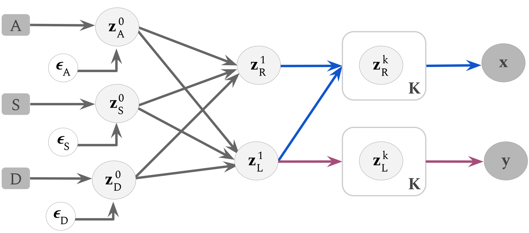
fig:subfigex [Direct Acyclic Graph (DAG)]  [Summarized Architecture]

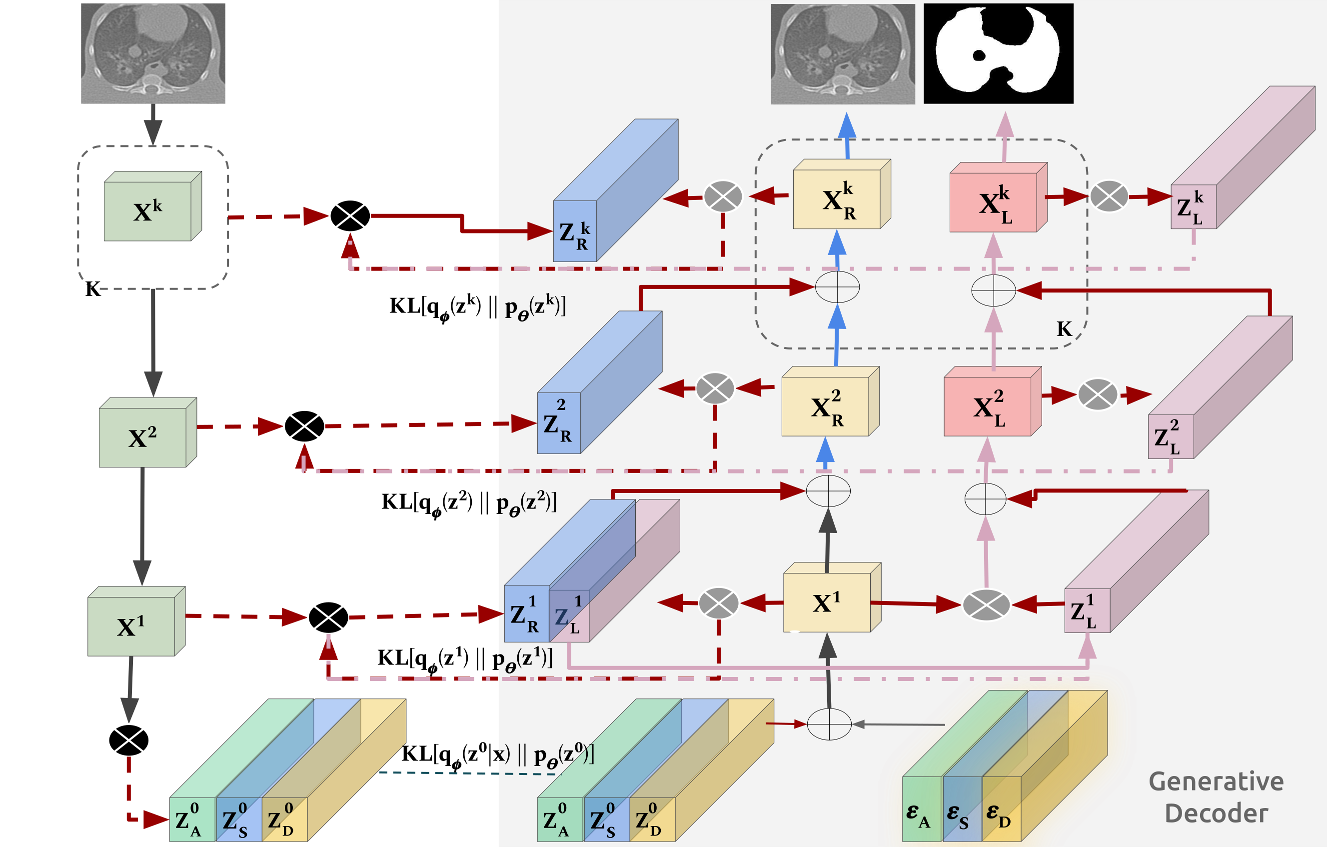
Figure 1: (a) Direct Acyclic Graph (DAG) representing the generation of pathological lung CT images $\operatorname*{\mathbf{x}}$, and their segmentation masks $\operatorname*{\mathbf{y}}$. Both generated from a latent variables hierarchy at different resolutions scales, $K$, governed by three factors, i.e., animal model, $A$, the relative position of the axial slice, $S$, and the estimated lung damage caused by Mtb., $D$. (b) Summarized architecture: Blue and pink represent the image and mask generation branches, $\bigoplus$ features concatenation and $\bigotimes$ $p_{\theta}$, $q_{\phi}$ parameters combination in training. The encoder is not present for image generation (Section 3.3). Counterfactual images arise inferring and setting some values at the deeper representation level $\mathbf{z}^{0}$ (Section 3.4).

The proposed DAG simplify the physical image generation for obvious reasons. All the possible elementary causative factors (e.g., specific scanner, comorbidities, subject age, sex) are reduced to three: the animal model, $A$, the observed lung axial slice, $S$, and the lung damage, $D$. The causative factors are modelled as three groups of independent variables, $\mathbf{z}^{0}$, under the noise term, $\epsilon_{\{A,S,D\}}$, which comprises noise and unconsidered variables. The primary variables govern the generative process, which follows a part-whole hierarchy [Hinton(2021)] from low-level representations of the texture and shape features, $\mathbf{z}^{1}$, to high dimensional ones, $\mathbf{z}^{k}$, the observed image, $\operatorname*{\mathbf{x}}$ and the segmentation mask, $\operatorname*{\mathbf{y}}$. This part-whole hierarchy resembles brain columns functioning [Locatello et al.(2020)Locatello, Weissenborn, Unterthiner, Mahendran, Heigold, Uszkoreit, Dosovitskiy, and Kipf, Devlin et al.(2018)Devlin, Chang, Lee, and Toutanova]. Variable superscripts, $\mathbf{z}^{k}$, symbolize hierarchy levels at the DAG.
The plate notation at the DAG represents such upsampling generation. The DAG implements two paths diverging at the first hierarchy level (shared representation path), $\mathbf{z}^{1}$. The division forces, during optimization, to generate a disentangled representation of shape, $\mathbf{z}_{L}$ and texture, $\mathbf{z}_{R}$. CT images depend on shape and texture variables (blue path), while the segmentation masks only depend on shape variables (pink path). Then, assuming the independence of the noise terms, the independent causal mechanism (ICM) principle is fulfilled [Scholkopf et al.(2021)Scholkopf, Locatello, Bauer, Ke, Kalchbrenner, Goyal, and Bengio] and the following disentangled factorization arise:

$$p(\operatorname*{\mathbf{x}},\operatorname*{\mathbf{y}},\operatorname*{\mathbf{z}})=p(\operatorname*{\mathbf{x}}|\mathbf{z}^{K}_{R})p(\operatorname*{\mathbf{y}}|\mathbf{z}^{K}_{L})p(\mathbf{z}_{R}^{k},)p(\mathbf{z}_{L}^{k})p(\mathbf{z}_{R}^{2}|\mathbf{z}_{R}^{1},\mathbf{z}_{L}^{1})p(\mathbf{z}_{R}^{1},\mathbf{z}_{L}^{1}|\mathbf{z}^{0})p(\mathbf{z}^{0}),$$ (1)

$$p(\mathbf{z}_{R}^{k})=\prod_{k=3}^{K}p(\mathbf{z}^{k}_{R}|\mathbf{z}^{k-1}_{R});\quad\qquad p(\mathbf{z}_{L}^{k})=\prod_{k=2}^{K}p(\mathbf{z}^{k}_{L}|\mathbf{z}^{k-1}_{L});\quad p(\mathbf{z^{0}})=p(\mathbf{z}_{A}^{0})p(\mathbf{z}_{S}^{0})p(\mathbf{z}_{D}^{0})$$ (2)

2.1 Model optimization

For the above equations, each conditional distribution is parametrized by depthwise convolutional decoders. The parameters $\theta$, leverages a high capacity model (fig:arq allowing to characterize the unobservable causes of variation ($\mathbf{\epsilon}$) consistent with the available data (in our case, lung CT images) [Peters et al.(2017)Peters, Janzing, and Schölkopf, Pawlowski et al.(2020)Pawlowski, Castro, and Glocker]. Once the model is optimized, it is possible to modify the disentangled variables to obtain new generated (3.3) and counterfactual images [Cohen et al.(2021)Cohen, Brooks, En, Zucker, Pareek, Lungren, and Chaudhari, Schutte et al.(2021)Schutte, Moindrot, Hérent, Schiratti, and Jégou](Section 3.4).

The computation of the parameters requires optimization through training of the posterior probability, $p_{\theta}(\operatorname*{\mathbf{z}}|\operatorname*{\mathbf{x}},\operatorname*{\mathbf{y}})$, which is intractable. To tackle this issue, we adapt the particular factorization in eq:factorization. We employ deep Variational Autoencoders (deep VAEs) with a bigger expressiveness than traditional VAEs [Kingma et al.(2016)Kingma, Salimans, Jozefowicz, Chen, Sutskever, and Welling, Child(2020)]. Thus, we can generate more detailed images and implement our hierarchical model.
In this way, we obtain the best approximate amortized posterior distribution, $q_{\phi}(z|x)$, being $\phi$ the parameters of the encoder. Notice that the distribution is amortized just from $\operatorname*{\mathbf{x}}$ (not from $\operatorname*{\mathbf{y}}$), so we force the model to extract the meaningful mechanism to generate the segmentation masks just from the self-supervisory signal of the image [LeCun and Misram Ishan(2021)]. Indeed, we add a segmentation branch in the architecture (fig:arq), dependent on the main branch.

Namely, we adopt the Noveau VAE (NVAE) [Vahdat and Kautz(2020)]. This architecture is carefully designed for hierarchical models. Moreover, it has proven efficacy in approximating posteriors by introducing an inductive bias in the image generating process in a deeply hierarchical architecture.

To this aim, the set of $\operatorname*{\mathbf{z}}$ variables at each representation level $k$ is divided into smaller sets, $m_{k}$, to get a total of $M$ groups of latent variables. Thus, a hierarchical structure is established within each resolution too, being $\operatorname*{\mathbf{z}}$ the set:

Its prior and approximate posterior probability are given by:

$$p_{\theta}(\operatorname*{\mathbf{z}})=\prod_{m}p_{\theta}(\mathbf{z}_{m}|\mathbf{z}_{m-1})\qquad q_{\phi}(\operatorname*{\mathbf{z}}|\operatorname*{\mathbf{x}})=\prod_{m}q_{\phi}(\mathbf{z}_{m}|\mathbf{z}_{m-1},\operatorname*{\mathbf{x}}).$$ (4)

Following this formulation, from marginalization of the $\log$ eq:factorization and rearranging terms, we obtain the variational lower bound to optimize (subscripts colors denote each optimization branch):

$$\small\mathcal{L(\operatorname*{\mathbf{x}},\operatorname*{\mathbf{y}})}=\mathbb{E}_{q_{\phi}({\color[rgb]{0,0,1}\operatorname*{\mathbf{z}}}|\operatorname*{\mathbf{x}})}\big{[}logp_{\theta}(\operatorname*{\mathbf{x}}|{\color[rgb]{0,0,1}\operatorname*{\mathbf{z}}})\big{]}-KL(q_{\phi}(\mathbf{z}_{0}|x)||p_{\theta}(\mathbf{z}_{0}))+\mathbb{E}_{q_{\phi}({\color[rgb]{1,0,1}\operatorname*{\mathbf{z}}}|\operatorname*{\mathbf{x}})}\big{[}logp_{\theta}(\operatorname*{\mathbf{y}}|{\color[rgb]{1,0,1}\operatorname*{\mathbf{z}}})\big{]}-\mathbb{E}_{{\color[rgb]{0,0,1}\operatorname*{\mathbf{z}}}}\big{[}KL_{{\color[rgb]{0,0,1}\operatorname*{\mathbf{z}}}}\big{]}-\mathbb{E}_{{\color[rgb]{1,0,1}\operatorname*{\mathbf{z}}}}\big{[}KL_{{\color[rgb]{1,0,1}\operatorname*{\mathbf{z}}}}\big{]}$$ (5)

$KL$ being the Kullback–Leibler divergence and

$$\small\mathbb{E}_{\operatorname*{\mathbf{z}}}\big{[}KL_{\operatorname*{\mathbf{z}}}\big{]}=\sum_{m}^{M}\mathbb{E}_{q_{\phi}(\mathbf{z_{m-1}}|\operatorname*{\mathbf{x}})}\big{[}KL(q_{\phi}(\mathbf{z}_{m}|\mathbf{z}_{m-1},\operatorname*{\mathbf{x}})||p_{\theta}(\mathbf{z}_{m}|\mathbf{z}_{m-1}))\big{]},$$ (6)

being $q_{\phi}(\mathbf{z}_{m-1}|\operatorname*{\mathbf{x}})$ the approximate posterior through the hierarchy of $m_{k-1}$ group.
Since NVAE convergence depends on the reasonable approximation of KL terms (see [Vahdat and Kautz(2020)]), to this aim, all priors and posterior probabilities are approximated as Normal distributions. Thus, we can write:

$$p(\mathbf{z}_{A}^{0})\sim\mathcal{N}(\mu(a),\sigma(a));\qquad p(\mathbf{z}_{S}^{0})\sim\mathcal{N}(\mu(s),\sigma(s));\qquad p(\mathbf{z}_{D}^{0})\sim\mathcal{N}(\mu(d),\sigma(d));$$ (7)

3 Experiments and Results

3.1 Datasets description

The model is optimized employing small datasets: ten lung CT volumes per animal model ($\sim 2000$ slices). The data used for training are axial slices from three Mtb. lung models identified as follows.

The dataset names identify: the animal model, $A$, the data source and the phase as follows $A_{phase}^{source}$). Namely, the human volumes, $H_{tr}^{CLE}$, corresponds to the validation data of the 2019 ImageClefMed TB task [Dicente Cid et al.(2019)Dicente Cid, Liauchuk, Klimuk, Tarasau, Kovalev, and Müller]. The mice images, $M_{tr}^{GSK}$, are provided from GlaxoSmithKline plc. (GSK) within the context of the ERA4TB project [ERA4TB consotium(2021)], similarly to the primate ones, $P_{tr}^{PHE}$, from the Public Health of England (PHE) [Gordaliza et al.(2018)Gordaliza, Muñoz-Barrutia, Abella, Desco, Sharpe, and Vaquero, Gordaliza et al.(2019)Gordaliza, Vaquero, Sharpe, Gleeson, and Muñoz-Barrutia]. For testing (twenty volumes per model), $P_{ts}^{PHE}$ and $M_{ts}^{GSK}$, are selected from different cohorts of $P_{tr}^{PHE}$ and $P_{tr}^{GSK}$, while the human dataset, $H_{ts}^{CLE}$ is a partition of the mentioned data. The remaining sets are included to evaluate the model generalisation and transferability capabilities. $M_{ts}^{EXM}$ belongs to a public dataset from the Institute for Experimental Molecular Imaging (ExMI) [Rosenhain et al.(2018)Rosenhain, Magnuska, Yamoah, Al Rawashdeh, Kiessling, and Gremse] which contains healthy subjects at low resolution. Finally, the human dataset, $H_{ts}^{RAD}$, presents subjects with lung damage caused by COVID-19 [Cohen et al.(2020)Cohen, Morrison, and Dao].

Note that all datasets include segmentation masks delineated by trained experts.

A detailed description of the different datasets is presented in tbl:datasets.

Table 1: Datasets description

Dataset ID	Phase	Animal Model	Source	# Slices	Voxel Spacing [mm]	Resolution
$M^{GSK}_{tr}$	Training			2002
$M^{GSK}_{ts}$			GSK	3987	$0.087\times 0.087$	$500\times 500$
$M^{EXM}_{ts}$	Test	Mouse	ExMI	3785	$0.282\times 0.282$	$144\times 100$
$P^{PHE}_{tr}$	Training			2012
$P^{PHE}_{ts}$	Test	Primate	PHE	4021	$0.235\times 0.235$	$512\times 512$
$H^{CLE}_{tr}$	Training			1617
$H^{CLE}_{ts}$			ImageClef	3578	$0.60\text{-}0.75\times 0.60\text{-}0.75$	$512\times 512$
$H^{RAD}_{ts}$	Test	Human	Radiopedia	4034	$0.68\text{-}0.75\times 0.68\text{-}0.75$	$512\text{-}630\times 430\text{-}630$

3.2 Implementation details

The model is optimized employing six scales, $K=6$, with $18$ latent variables per scale, partitioned each in $m_{k}$ groups as follows, $m_{k}=[2,2,2,3,6,9]$. The three $\mu_{A}$, $\mu_{S}$ and $\mu_{D}$ are known during training ($\mu_{A}=[-1,0,1]$, $\mu_{D}=(0,1)$, $\mu_{S}=(0,1)$), fix at image generation and inferred for image reconstruction and segmentation mask generation employing $KL\big{(}q_{\phi}(z^{0})||\mathcal{N}(0,1)\big{)}$. During optimization $\mu_{D}$ is given by the the healthy lung relative volume (extracted by simple thresholding) with respect to the ground truth mask volume.

3.3 Pathological Lungs Generation

After optimization, the model can generate realistic images, such as those shown in fig:generated, by choosing the mean values of $\mathbf{z}_{A}^{0}$, $\mathbf{z}_{S}^{0}$, $\mathbf{z}_{D}^{0}$ factors. To illustrate this capacity in fig:generated, we set a relative slice position of $0.5$, the animal model is fixed for each row and, the effect of the lung damage variable is modulated from lower to higher in each column.

fig:generated

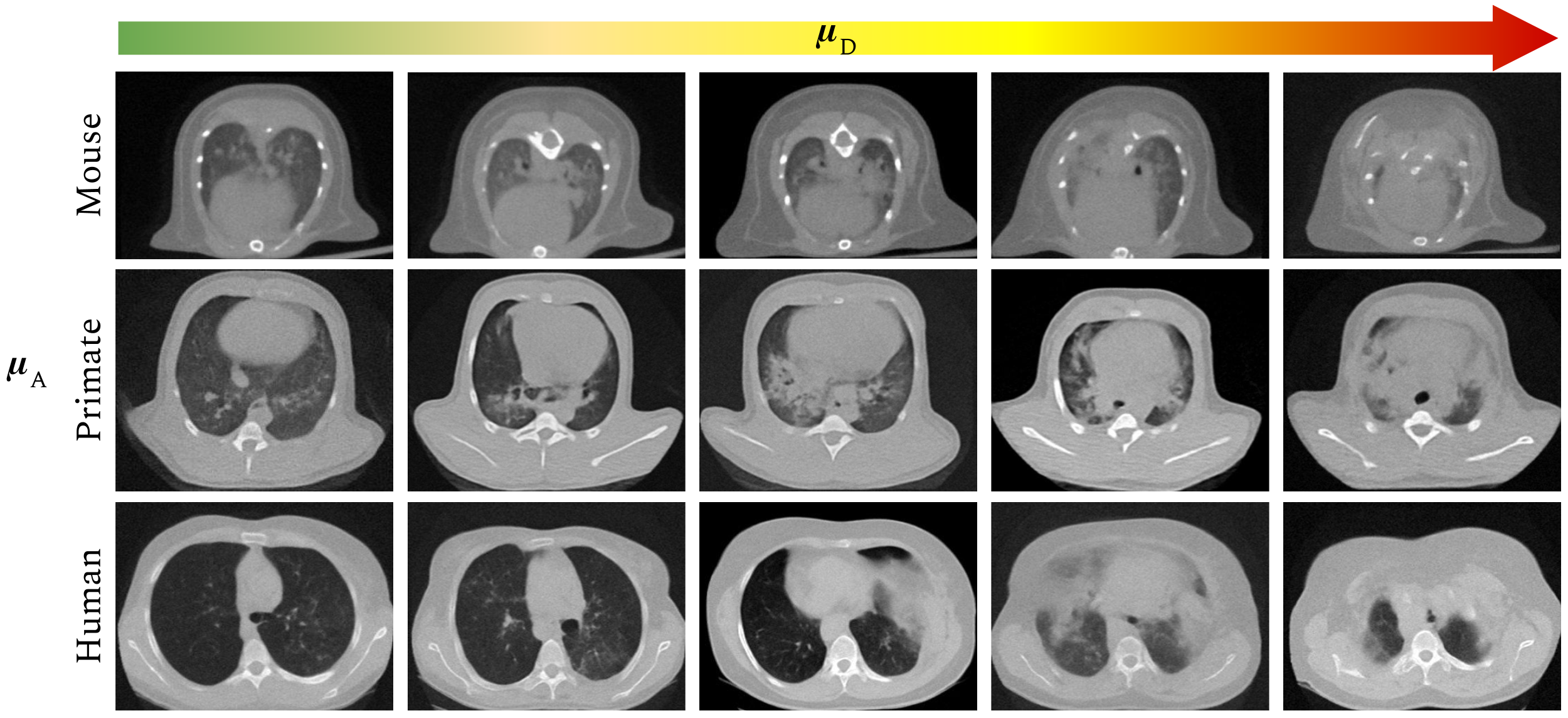
Figure 2: Synthetic lung CT images generated by our model. Images are generated with a fixed slice relative position ($\mu_{S}$). For each row, the animal model $\mu_{A}$ is fixed to $-1,0,1$, respectively, while for each column, the damage $\mu_{D}$ is increased [$0$-$1$].

3.4 Counterfactual Images

The first column of each row in fig:counter shows an actual image of a damaged lung corresponding to a given animal model. When no actions are performed, the model infers the disentangled image representation of the causative variables ($\mathbf{z}_{A}^{0}$, $\mathbf{z}_{S}^{0}$, $\mathbf{z}_{D}^{0}$) through the encoder. Subsequently, the image is reconstructed, and a segmentation mask (third column) is generated employing the optimized decoder (fig:arq). The second column shows a healthy counterfactual of the input images, which is generated setting to zero the mean value of the inferred damage variable, $\mathbf{z_{D}^{0}}$. The decoder is fed with the zero-mean $\mathbf{z_{D}^{0}}$ and the rest (unaltered) inferred causal variables to generate the counterfactual version of the slice and its respective mask (fourth column).

fig:counter

Figure 3: The encoder infers the real image (axial slice) disentangled representation, $\mathbf{z}_{A}^{0}$, $\mathbf{z}_{S}^{0}$, $\mathbf{z}_{D}^{0}$. By setting the damage variable $\mathbf{z}_{D}^{0}$ to $0$ the decoder generates the healthy counterfactual (counterfactual slice) and its respective mask (counterfactual mask).

3.5 Segmentation employing counterfactual images

Pathological lung segmentation is an important task to solve in drug development studies. Unfortunately, it is a complex task due to the difficulty of discrimination between lesions and other neighborhood tissues. Needless to say that the diversity of the biological data supposes an added difficulty[Hofmanninger et al.(2020)Hofmanninger, Prayer, Pan, Röhrich, Prosch, and Langs]. In this experiment, we retrain the optimized model with counterfactual images to generate the segmentation masks from the test datasets (Section 3.1). We use the approach described previously to generate the counterfactual images (Section 3.4). To learn about the strengths and weaknesses of this generative approach, we compare the results obtained, $our_{c}$, with the segmentation masks calculated by our original method, $our_{nc}$, and the state-of-the-art fully supervised method, nnU-Nnet [Isensee et al.(2021)Isensee, Jaeger, Kohl, Petersen, and Maier-Hein].

Table 2: Mean and standard deviation (SD) of the Dice Similarity Coefficient (DSC) and Hausdorff Distance (HD) between the ground truth masks and mask obtained from the methods indicated at rows (nnU-Nnet, proposed method before employing counterfactual images ($our_{nc}$), and after ($our_{c}$)) for each test dataset (columns).

	DSC $\pm$ SD					HD $\pm$ SD [mm]
	$M^{GSK}_{ts}$	$M^{EXT}_{ts}$	$P^{PHE}_{ts}$	$H^{CLE}_{ts}$	$H^{COV}_{ts}$	$M^{GSK}_{ts}$	$M^{EXM}_{ts}$	$P^{PHE}_{ts}$	$H^{CLE}_{ts}$	$H^{COV}_{ts}$
nnU-Net	$0.845\pm 0.10$	$0.851\pm 0.11$	$0.957\pm 0.06$	$0.978\pm 0.04$	$0.973\pm 0.03$	$1.737\pm 1.01$	$1.90\pm 1.52$	$3.30\pm 3.96$	$9.37\pm 15.14$	$8.31\pm 10.71$
$our_{nc}$	$0.849\pm 0.10$	$0.843\pm 0.12$	$0.949\pm 0.06$	$0.963\pm 0.06$	$0.963\pm 0.06$	$1.948\pm 1.11$	$2.06\pm 1.82$	$3.81\pm 4.10$	$10.12\pm 18.32$	$10.56\pm 10.77$
$our_{c}$	$0.877\pm 0.08$	$0.859\pm 0.11$	$0.955\pm 0.06$	$0.977\pm 0.06$	$0.968\pm 0.04$	$1.519\pm 0.89$	$1.88\pm 1.53$	$2.95\pm 3.54$	$8.78\pm 16.11$	$9.48\pm 9.89$

tbl:optimiza_results shows the mean and standard deviation for Dice Similarity Coefficient (DSC) and Hausdorff Distance (HD) between each segmentation method and the ground truth masks for each test dataset. The results present an improvement for all measures and datasets when employing counterfactual images, yielding similar results to the nnU-Nnet. The differences are due to subtle changes in most of the cases or even small imperfections in the ground truth masks as it is shown in fig:lungs_seg.

fig:lungs_seg

Figure 4: Comparison of methods. Each row contains axial slices and segmentation masks of each test dataset. Columns show the original image, ground truth mask (green), nnU-Net mask (blue), overlay of nnU-Net and ground truth (cyan), the mask with our method employing counterfactual images during training (yellow) and the overlay with the ground truth (lime). Red and green circles show inaccuracies and precise segmentation cases, respectively.

4 Conclusions

The methodology proposed in this work yields promising results obtaining the factors characterizing the pathophysiological processes shared between animal models. Although the approach indeed suffers from several limitations: the use of isolated axial slices instead of the more informative whole three-dimensional images and the characterization of disease affectation based simply on the damaged lung volume and not on the specific manifestations of the disease for each animal model. These limitations will be the object of future work.

To sum up, our model is capable of inferring meaningful disentangled representations. Namely, it generates synthetic slices by setting the values of the modelled factors. Even more relevant, it produces counterfactual versions of existing slices by testing the effective disentanglement. In the future, we explore strategies to exploit the approach to increase the diversity of existing data, essential for automatic segmentation, or to provide the damage variable as a possible (to be validated) inter-species biomarker.

This project has received funding from the Innovative Medicines Initiative 2 Joint Undertaking (JU) under grant agreement No. 853989. The JU receives support from the European Union’s Horizon 2020 research and innovation programme and EFPIA and Global Alliance for TB Drug Development non-profit organisation, Bill & Melinda Gates Foundation and University of Dundee. This work was partially funded by Ministerio de Ciencia, Innovación y Universidades, Agencia Estatal de Investigación, under grant PID2019-109820RB-I00, MCIN/AEI/10.13039/501100011033/, co-finance by European Regional Development Fund (ERDF), “A way of making Europe.”

Appendix A Life cycle of Tuberculosis infection

Figure 5: Life cycle of Mtb. [Arroyo-Ornelas et al.(2012)Arroyo-Ornelas, Arenas-Arrocena, Estrada, Castaño, and López-Marín, Ernst(2012)] and main tests to characterise the entire disease spectrum. The inner cycle names the traditional categorical clinical stages of the continuous spectrum of TB immunological life cycle. Each outer circle represent each TB assessment tests capability. Blank spaces for lack of sensibility, bicolour ones represent the binary character of the test, while gradient representation represents the ability to provide a continuous value.

Appendix B Extra Experiments Setup details

The following list offers further details about the context of the experiments.

• System setup: All experiments were performed in a machine with an Intel Xeon 8153 CPU, 64-GB RAM and two 12-GB Titan V GPUs. We created a specific Docker image based on Ubuntu 20.04 with Python 3.6.9 and torch 1.6.0 to run our code.

• Preprocessing: To reduce the size of the chest CT images, we crop the images and their respective segmentation masks to the body region. We employ thresholding from $-1024$ to $600$ over the Hounsfield Units (HU) followed by morphological operations to eliminate small isolated blobs. Finally, we select the one corresponding to the whole body region.

  Since nnU-Net automatically estimates the rest of preprocessing operations, these cropped volumes feed the nnU-Net preprocessing pipelines. The details about nnU-Net experiments are given below in the list.

  In the case of our model, we rescale the cropped images resolution to 256 x 256 pixels and normalize the intensity (0-1).

  During training, our model needs an estimation of healthy lung volume per CT (Sections 2 and 3.2). To this aim, over the cropped image, we apply a threshold to recover just the healthy tissue inside the whole lung mask. Following the experts’ recommendations, we set this threshold from $-900$ to $-200$ HUs for the human training dataset ($H^{CLE}_{tr}$), -1000 to -200 HUs for the macaque dataset ($P^{PHE}_{tr}$), and from -800 to -300 HUs for the mouse model ($M^{GSK}_{tr}$). The healthy volume extracted is divided by the total mask volume to obtain the relative value employed during training.

• Selection of each dataset sample: We use $30$ CT volumes per dataset employed during training and testing and $20$ when the datasets are employed just during the test phase, as described in Section 3.1.

  Except for the $M^{GSK}$ and $H^{RAD}$ datasets, the rest of the original datasets contain more than $30/20$ volumes.

  To define our specific trimmed samples, we employ the relative healthy volume to classify each CT as low damage (relative healthy volume $\geq 0.85$), medium damage ($0.85>$ relative healthy volume $>0.4$) and high damage (relative healthy volume $\leq 0.4$). Subsequently, we randomly select the same number of subjects per interval.

• Training details: We employ the two Titan V GPUs during $900$ epochs with a total batch size of $8$ using the Adamax optimizer with an initial learning rate of $0.01$ and Cosine Annealing scheduler (minimal learning rate: $1e-4$). We apply online data augmentation to the normalized images by employing random affine transformations (10º rotation) and adding Gaussian noise ($\mu=0$, $\sigma=0.05$).

  For the nnU-Net [Isensee et al.(2021)Isensee, Jaeger, Kohl, Petersen, and Maier-Hein], we use a single Titan V GPU, following the nnU-Net authors’ (https://github.com/MIC-DKFZ/nnUNetrecommendations). After adapting the cropped image name formats to the nnU-Net requirements, we run the nnUNet_plan_and_preprocess function to allow the pipeline to estimate the network configuration and training parameters. The complete list can be found in the following https://drive.google.com/file/d/1-fmQ_tt1ElHhO6rHMzsUG7QYLaOszn5C/view?usp=sharinglink. Subsequently, we train a 2D configuration in a 5-fold cross-validation during $1000$ epochs per fold, employing a batch size of $14$, data augmenting (see https://drive.google.com/file/d/1-fmQ_tt1ElHhO6rHMzsUG7QYLaOszn5C/view?usp=sharinglinked file for details), the SGD optimizer and a learning rate of $0.01$

• Image Generation speed: After loading the trained model ($\sim 20s$), it is possible to generate a 16 batch size of $256\times 256$ images in approximately 0.25s.

Appendix C Pathological Lungs Generation: Varying the slice position

This appendix shows generated slices instances fixing the damage and varying the relative slice position. This experiment extends Section 3.3, in which axial slices belong to a fixed relative slice position.

Since our chest CT volumes orientation is cephalic to caudal, the model generates axial images of the upper airways (trachea) and the corresponding per animal model surrounding tissues at the lowest slice position, as shown in the first column of the fig:generated_vary. This way, the second column shows the corresponding generated anatomy for the superior lungs, while the third and fourth columns accordingly show the middle and inferior regions. Finally, the fifth column depicts the generated version at the beginning of the abdominal anatomy.

fig:generated_vary

Figure 6: Synthetic lung CT images generated by our model. Images are generated with a fix relative damage, $\mu_{D}=0.5$. For each row, the animal model $\mu_{A}$ is fixed to $-1,0,1$, respectively, while for each column, the relative slice position $\mu_{S}$ is increased between $0$ and $1$.

Appendix D Counterfactual Images: Extended Assessment

This appendix extends the qualitative results presented in Section 3.4. The former section shows the model capacity generating counterfactual images and their respective segmentation masks.

Here, we evaluate how realistic are the generated images. For that, we compare the Hounsfield Units (HU) of real CT slices with two cases: a) the reconstructed slice from the variable inferred by the encoder without modification of any of these values, and b) the counterfactual image, namely, after intervening on the inferred damage value. We compute the voxel-wise Root Mean Square Error (RMSE) for the reconstructed images per test dataset. tbl:RMSE shows these results with an average $RMSE=18.73\pm 2.16$.

Voxel-wise evaluation is not suitable for counterfactual images. Previous manual delimitation of comparable regions is needed, which is a priority for our future work.

To illustrate similarities and differences in the HU scale, in fig:profiles, we plot the HU profile belonging to the damaged regions shown in fig:counter. Respectively, the first three rows contain 1) the original axial slice from the different test datasets (the image is generated from the $\mu_{a}$, $\mu_{s}$ and $\mu_{d}$ inferred by our model), with the profile horizontal line in green, 2) the reconstructed slice (the image is generated maintaining $\mu_{a}$, $\mu_{s}$ inferred by our model and correcting $\mu_{d}$), with profile line in yellow and 3) the counterfactual after modifying the inferred expected damage, with the profile line in blue.

The last row shows the HU plot for each profile-specific colour. HU values are similar for the three slices except for those regions where the slice counterfactual version replaces the damage with healthy tissue-like. We highlight such changes framing them in vertical dashed red lines.

Besides, it is important to note that the original and reconstructed images present more noisy patterns than the counterfactual version, as was expected from its blurrier appearance and the thickening of the soft tissue for the mice dataset.

Table 3: Root Mean Square Error (RMSE) between the real images and the image reconstructed from the $\mu_{a}$, $\mu_{s}$ and $\mu_{d}$ inferred by our model for the test datasets

RMSE [HU]
$M^{GSK}_{ts}$	$M^{EXT}_{ts}$	$P^{PHE}_{ts}$	$H^{CLE}_{ts}$	$H^{COV}_{ts}$
$21.26$	$18.75$	$20.12$	$17.89$	$15.63$

fig:profiles

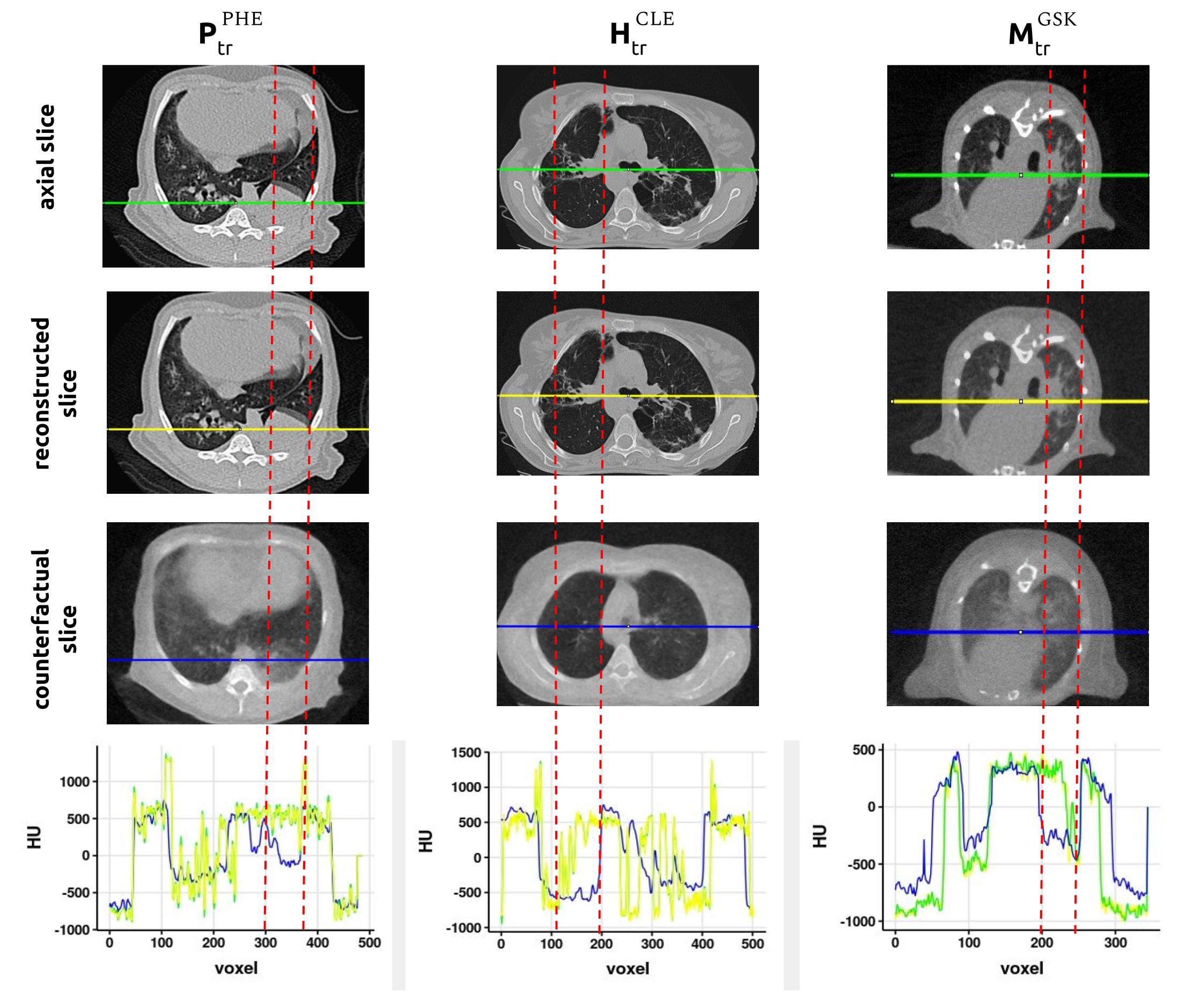
Figure 7: Hounsfield Units (HU) plots for profiles at regions damaged in original test axial slices. Each column contains instances of each dataset, previously employed in Section 3.4. The first rows depict the original, reconstructed and counterfactual slices with the profile line green, yellow and blue, respectively. The last row draws the HU profiles per voxel. Vertical dashed lines highlight big differences between real/reconstructed and counterfactual slices.

References

- [Arjovsky et al.(2020)Arjovsky, Bottou, Gulrajani, and Lopez-Paz] Martin Arjovsky, Léon Bottou, Ishaan Gulrajani, and David Lopez-Paz. Invariant Risk Minimization. In ArXiv, 7 2020. URL http://arxiv.org/abs/1907.02893 http://arxiv.org/abs/2002.04692.
- [Arroyo-Ornelas et al.(2012)Arroyo-Ornelas, Arenas-Arrocena, Estrada, Castaño, and López-Marín] Miguel A. Arroyo-Ornelas, Ma. Concepción Arenas-Arrocena, Horacio V. Estrada, Victor M. Castaño, and Luz M. López-Marín. Immune Diagnosis of Tuberculosis Through Novel Technologies. In Understanding Tuberculosis - Global Experiences and Innovative Approaches to the Diagnosis. IntechOpen, 2 2012. ISBN 978-953-307-938-7. 10.5772/31421. URL https://www.intechopen.com/chapters/28548.
- [Bengio et al.(2013)Bengio, Courville, and Vincent] Yoshua Bengio, Aaron Courville, and Pascal Vincent. Representation learning: A review and new perspectives. IEEE Transactions on Pattern Analysis and Machine Intelligence, 35(8):1798–1828, 2013. 10.1109/TPAMI.2013.50.
- [Castro et al.(2020)Castro, Walker, and Glocker] Daniel C. Castro, Ian Walker, and Ben Glocker. Causality matters in medical imaging. Nature Communications, 11(1):1–10, 12 2020. ISSN 20411723. 10.1038/s41467-020-17478-w. URL https://doi.org/10.1038/s41467-020-17478-w.
- [Child(2020)] Rewon Child. Very Deep VAEs Generalize Autoregressive Models and Can Outperform Them on Images. 11 2020. URL https://arxiv.org/abs/2011.10650v2.
- [Cohen et al.(2020)Cohen, Morrison, and Dao] Joseph Paul Cohen, Paul Morrison, and Lan Dao. COVID-19 Image Data Collection, 3 2020. ISSN 2331-8422. URL https://academictorrents.com/details/136ffddd0959108becb2b3a86630bec049fcb0ff.
- [Cohen et al.(2021)Cohen, Brooks, En, Zucker, Pareek, Lungren, and Chaudhari] Joseph Paul Cohen, Rupert Brooks, Sovann En, Evan Zucker, Anuj Pareek, Matthew P. Lungren, and Akshay Chaudhari. Gifsplanation via Latent Shift: A Simple Autoencoder Approach to Counterfactual Generation for Chest X-rays. Proceedings of Machine Learning Research, 2021. URL https://mlmed.org/gifsplanation/ http://arxiv.org/abs/2102.09475.
- [DeGrave et al.(2021)DeGrave, Janizek, and Lee] Alex J. DeGrave, Joseph D Janizek, and Su In Lee. AI for radiographic COVID-19 detection selects shortcuts over signal. Nature Machine Intelligence, 3(7):2020.09.13.20193565, 10 2021. 10.1038/s42256-021-00338-7. URL https://doi.org/10.1101/2020.09.13.20193565.
- [Devlin et al.(2018)Devlin, Chang, Lee, and Toutanova] Jacob Devlin, Ming Wei Chang, Kenton Lee, and Kristina Toutanova. BERT: Pre-training of Deep Bidirectional Transformers for Language Understanding. NAACL HLT 2019 - 2019 Conference of the North American Chapter of the Association for Computational Linguistics: Human Language Technologies - Proceedings of the Conference, 1:4171–4186, 10 2018. URL https://arxiv.org/abs/1810.04805v2.
- [Dicente Cid et al.(2019)Dicente Cid, Liauchuk, Klimuk, Tarasau, Kovalev, and Müller] Yashin Dicente Cid, Vitali Liauchuk, Dzmitri Klimuk, Aleh Tarasau, Vassili Kovalev, and Henning Müller. Overview of ImageCLEFtuberculosis 2019 - Automatic CT-based Report Generation and Tuberculosis Severity Assessment. In Proceedings of CLEF (Conference and Labs of the Evaluation Forum) 2019 Working Notes. CEUR-WS.org, 2019. URL http://ceur-ws.org/Vol-2380/paper_138.pdf.
- [Dumoulin and Visin(2018)] Vincent Dumoulin and Francesco Visin. A guide to convolution arithmetic for deep learning. 3 2018. URL https://arxiv.org/abs/1603.07285v2 http://arxiv.org/abs/1603.07285.
- [ERA4TB consotium(2021)] ERA4TB consotium. ERA4TB, 2021. URL https://era4tb.org/the-project/.
- [Ernst(2012)] Joel D. Ernst. The immunological life cycle of tuberculosis. Nature Reviews Immunology 2012 12:8, 12(8):581–591, 7 2012. ISSN 1474-1741. 10.1038/nri3259. URL https://www.nature.com/articles/nri3259.
- [Gordaliza et al.(2018)Gordaliza, Muñoz-Barrutia, Abella, Desco, Sharpe, and Vaquero] Pedro M. Gordaliza, Arrate Muñoz-Barrutia, Mónica Abella, Manuel Desco, Sally Sharpe, and Juan José Vaquero. Unsupervised CT Lung Image Segmentation of a Mycobacterium Tuberculosis Infection Model. Scientific Reports, 8(1), 12 2018. ISSN 2045-2322. 10.1038/s41598-018-28100-x. URL http://www.nature.com/articles/s41598-018-28100-x.
- [Gordaliza et al.(2019)Gordaliza, Vaquero, Sharpe, Gleeson, and Muñoz-Barrutia] Pedro M. Gordaliza, Juan José Vaquero, Sally Sharpe, Fergus Gleeson, and Arrate Muñoz-Barrutia. A Multi-Task Self-Normalizing 3D-CNN to Infer Tuberculosis Radiological Manifestations. In Medical Imaging with Deep Learning (MIDL), pages 1–5, 7 2019. URL http://arxiv.org/abs/1907.12331.
- [Goyal and Bengio(2021)] Anirudh Goyal and Yoshua Bengio. Inductive Biases for Deep Learning of Higher-Level Cognition. 11 2021. URL http://arxiv.org/abs/2011.15091.
- [Hinton(2018)] Geoffrey Hinton. Deep Learning—A Technology With the Potential to Transform Health Care. JAMA, 320(11):1101, 9 2018. ISSN 0098-7484. 10.1001/jama.2018.11100. URL http://jama.jamanetwork.com/article.aspx?doi=10.1001/jama.2018.11100.
- [Hinton(2021)] Geoffrey Hinton. How to represent part-whole hierarchies in a neural network. 2 2021. URL http://arxiv.org/abs/2102.12627.
- [Hofmanninger et al.(2020)Hofmanninger, Prayer, Pan, Röhrich, Prosch, and Langs] Johannes Hofmanninger, Forian Prayer, Jeanny Pan, Sebastian Röhrich, Helmut Prosch, and Georg Langs. Automatic lung segmentation in routine imaging is primarily a data diversity problem, not a methodology problem. European Radiology Experimental, 4(1), 12 2020. ISSN 25099280. 10.1186/s41747-020-00173-2. URL /pmc/articles/PMC7438418/?report=abstract https://www.ncbi.nlm.nih.gov/pmc/articles/PMC7438418/.
- [Isensee et al.(2021)Isensee, Jaeger, Kohl, Petersen, and Maier-Hein] Fabian Isensee, Paul F. Jaeger, Simon A.A. Kohl, Jens Petersen, and Klaus H. Maier-Hein. nnU-Net: a self-configuring method for deep learning-based biomedical image segmentation. Nature Methods, 18(2):203–211, 2 2021. ISSN 15487105. 10.1038/s41592-020-01008-z. URL https://www.nature.com/articles/s41592-020-01008-z.
- [Kingma et al.(2016)Kingma, Salimans, Jozefowicz, Chen, Sutskever, and Welling] Diederik P. Kingma, Tim Salimans, Rafal Jozefowicz, Xi Chen, Ilya Sutskever, and Max Welling. Improving Variational Inference with Inverse Autoregressive Flow. (Nips), 2016. ISSN 10495258. URL http://arxiv.org/abs/1606.04934.
- [LeCun and Misram Ishan(2021)] Yann LeCun and Misram Ishan. Self-supervised learning: The dark matter of intelligence, 3 2021. URL https://ai.facebook.com/blog/self-supervised-learning-the-dark-matter-of-intelligence/.
- [Liu et al.(2021)Liu, Sanchez, Thermos, O’Neil, and Tsaftaris] Xiao Liu, Pedro Sanchez, Spyridon Thermos, Alison Q. O’Neil, and Sotirios A. Tsaftaris. A Tutorial on Learning Disentangled Representations in the Imaging Domain. 8 2021. URL https://arxiv.org/abs/2108.12043v1.
- [Locatello et al.(2020)Locatello, Weissenborn, Unterthiner, Mahendran, Heigold, Uszkoreit, Dosovitskiy, and Kipf] Francesco Locatello, Dirk Weissenborn, Thomas Unterthiner, Aravindh Mahendran, Georg Heigold, Jakob Uszkoreit, Alexey Dosovitskiy, and Thomas Kipf. Object-Centric Learning with Slot Attention. Advances in Neural Information Processing Systems, 2020-December, 6 2020. ISSN 10495258. URL https://arxiv.org/abs/2006.15055v2.
- [Pai et al.(2016)Pai, Behr, Dowdy, Dheda, Divangahi, Boehme, Ginsberg, Swaminathan, Spigelman, Getahun, Menzies, and Raviglione] Madhukar Pai, Marcel A. Behr, David Dowdy, Keertan Dheda, Maziar Divangahi, Catharina C. Boehme, Ann Ginsberg, Soumya Swaminathan, Melvin Spigelman, Haileyesus Getahun, Dick Menzies, and Mario Raviglione. Tuberculosis. Nature Reviews Disease Primers, 2:1–23, 2016. ISSN 2056676X. 10.1038/nrdp.2016.76. URL http://dx.doi.org/10.1038/nrdp.2016.76.
- [Pawlowski et al.(2020)Pawlowski, Castro, and Glocker] Nick Pawlowski, Daniel C. Castro, and Ben Glocker. Deep Structural Causal Models for Tractable Counterfactual Inference. In Neural Information Processing Systems (NIPS), 6 2020. URL http://arxiv.org/abs/2006.06485.
- [Pearl(2011)] Judea Pearl. Causality: Models, reasoning, and inference, second edition. 2011. ISBN 9780511803161. 10.1017/CBO9780511803161.
- [Peters et al.(2017)Peters, Janzing, and Schölkopf] Jonas Peters, Dominik Janzing, and Bernhard Schölkopf. Elements of Causal Inference: Foundations and Learning Algorithms. The MIT Press, London, England, 2017. ISBN 9780262037310. URL http://web.math.ku.dk/ peters/.
- [Roberts et al.(2021)Roberts, Driggs, Thorpe, Gilbey, Yeung, Ursprung, Aviles-Rivero, Etmann, McCague, Beer, Weir-McCall, Teng, Gkrania-Klotsas, Ruggiero, Korhonen, Jefferson, Ako, Langs, Gozaliasl, Yang, Prosch, Preller, Stanczuk, Tang, Hofmanninger, Babar, Sánchez, Thillai, Gonzalez, Teare, Zhu, Patel, Cafolla, Azadbakht, Jacob, Lowe, Zhang, Bradley, Wassin, Holzer, Ji, Ortet, Ai, Walton, Lio, Stranks, Shadbahr, Lin, Zha, Niu, Rudd, Sala, and Schönlieb] Michael Roberts, Derek Driggs, Matthew Thorpe, Julian Gilbey, Michael Yeung, Stephan Ursprung, Angelica I. Aviles-Rivero, Christian Etmann, Cathal McCague, Lucian Beer, Jonathan R. Weir-McCall, Zhongzhao Teng, Effrossyni Gkrania-Klotsas, Alessandro Ruggiero, Anna Korhonen, Emily Jefferson, Emmanuel Ako, Georg Langs, Ghassem Gozaliasl, Guang Yang, Helmut Prosch, Jacobus Preller, Jan Stanczuk, Jing Tang, Johannes Hofmanninger, Judith Babar, Lorena Escudero Sánchez, Muhunthan Thillai, Paula Martin Gonzalez, Philip Teare, Xiaoxiang Zhu, Mishal Patel, Conor Cafolla, Hojjat Azadbakht, Joseph Jacob, Josh Lowe, Kang Zhang, Kyle Bradley, Marcel Wassin, Markus Holzer, Kangyu Ji, Maria Delgado Ortet, Tao Ai, Nicholas Walton, Pietro Lio, Samuel Stranks, Tolou Shadbahr, Weizhe Lin, Yunfei Zha, Zhangming Niu, James H.F. Rudd, Evis Sala, and Carola Bibiane Schönlieb. Common pitfalls and recommendations for using machine learning to detect and prognosticate for COVID-19 using chest radiographs and CT scans. Nature Machine Intelligence, 3(3):199–217, 3 2021. ISSN 25225839. 10.1038/s42256-021-00307-0. URL https://doi.org/10.1038/s42256-021-00307-0.
- [Rosenhain et al.(2018)Rosenhain, Magnuska, Yamoah, Al Rawashdeh, Kiessling, and Gremse] Stefanie Rosenhain, Zuzanna A. Magnuska, Grace G. Yamoah, Wa’El Al Rawashdeh, Fabian Kiessling, and Felix Gremse. A preclinical micro-computed tomography database including 3D whole body organ segmentations. Scientific Data, 5(1):1–9, 12 2018. ISSN 20524463. 10.1038/sdata.2018.294.
- [Scholkopf et al.(2021)Scholkopf, Locatello, Bauer, Ke, Kalchbrenner, Goyal, and Bengio] Bernhard Scholkopf, Francesco Locatello, Stefan Bauer, Nan Rosemary Ke, Nal Kalchbrenner, Anirudh Goyal, and Yoshua Bengio. Toward Causal Representation Learning. Proceedings of the IEEE, 109(5):612–634, 5 2021. ISSN 15582256. 10.1109/JPROC.2021.3058954.
- [Schutte et al.(2021)Schutte, Moindrot, Hérent, Schiratti, and Jégou] Kathryn Schutte, Olivier Moindrot, Paul Hérent, Jean-Baptiste Schiratti, and Simon Jégou. Using StyleGAN for Visual Interpretability of Deep Learning Models on Medical Images. 1 2021. URL https://arxiv.org/abs/2101.07563v1.
- [Vahdat and Kautz(2020)] Arash Vahdat and Jan Kautz. NVAE: A Deep Hierarchical Variational Autoencoder. Advances in Neural Information Processing Systems, 2020-Decem, 7 2020. ISSN 10495258. URL https://arxiv.org/abs/2007.03898v3.
- [Willmann et al.(2008)Willmann, van Bruggen, Dinkelborg, and Gambhir] Jürgen K Willmann, Nicholas van Bruggen, Ludger M Dinkelborg, and Sanjiv S Gambhir. Molecular imaging in drug development. Nature Reviews Drug Discovery, 7(7):591–607, 2008.
- [Yang et al.(2021)Yang, Wang, Wen, Weiner, and Via] Hee-Jeong Yang, Decheng Wang, Xin Wen, Danielle M. Weiner, and Laura E. Via. One Size Fits All? Not in In Vivo Modeling of Tuberculosis Chemotherapeutics. Frontiers in Cellular and Infection Microbiology, 0:134, 3 2021. ISSN 2235-2988. 10.3389/FCIMB.2021.613149.
- [Zhou et al.(2021)Zhou, Greenspan, Davatzikos, Duncan, van Ginneken, Madabhushi, Prince, Rueckert, and Summers] S. Kevin Zhou, Hayit Greenspan, Christos Davatzikos, James S. Duncan, Bram van Ginneken, Anant Madabhushi, Jerry L. Prince, Daniel Rueckert, and Ronald M. Summers. A Review of Deep Learning in Medical Imaging: Imaging Traits, Technology Trends, Case Studies With Progress Highlights, and Future Promises. Proceedings of the IEEE, pages 1–19, 2021. ISSN 0018-9219. 10.1109/JPROC.2021.3054390. URL https://ieeexplore.ieee.org/document/9363915/.