Tail-GAN:
Learning to Simulate Tail Risk Scenarios

Abstract

The estimation of loss distributions for dynamic portfolios requires the simulation of scenarios representing realistic joint dynamics of their components, with particular importance devoted to the simulation of tail risk scenarios. We propose a novel data-driven approach that utilizes Generative Adversarial Network (GAN) architecture and exploits the joint elicitability property of Value-at-Risk (VaR) and Expected Shortfall (ES). Our proposed approach is capable of learning to simulate price scenarios that preserve tail risk features for benchmark trading strategies, including consistent statistics such as VaR and ES.

We prove a universal approximation theorem for our generator for a broad class of risk measures. In addition, we show that the training of the GAN may be formulated as a max-min game, leading to a more effective approach for training. Our numerical experiments show that, in contrast to other data-driven scenario generators, our proposed scenario simulation method correctly captures tail risk for both static and dynamic portfolios.

Keywords: Scenario simulation, Generative adversarial networks (GAN), Time series, Universal approximation, Expected shortfall, Value at risk, Risk measures, Elicitability.

1 Introduction

Scenario simulation is extensively used in finance for evaluating the loss distribution of portfolios and trading strategies, often with a focus on the estimation of risk measures such as Value-at-Risk and Expected Shortfall (Glasserman [2003]). The estimation of such risk measures for static and dynamic portfolios involves the simulation of scenarios representing realistic joint dynamics of their components. This requires both a realistic representation of the temporal dynamics of individual assets (temporal dependence), as well as an adequate representation of their co-movements (cross-asset dependence).

Risk estimation has become increasingly important in financial applications in recent years, in light of the Basel Committee’s Fundamental Review of the Trading Book (FRTB), an international standard that regulates the amount of capital banks ought to hold against market risk exposures (see Bank for International Settlements [2019]). FRTB particularly revisits and emphasizes the use of Value-at-Risk vs Expected Shortfall (Du and Escanciano [2017]) as a measure of risk under stress, thus ensuring that banks appropriately capture tail risk events. In addition, FRTB requires banks to develop clear methodologies to specify how various extreme scenarios are simulated, and how the stress scenario risk measures are constructed using these scenarios. This suite of capital rules has taken effect January 2022 to strengthen the financial system, with an eye towards capturing tail risk events that came to light during the 2007-2008 financial crisis.

A common approach in scenario simulation is to use parametric models. The specification and estimation of such parametric models poses challenges in situations in which one is interested in heterogeneous portfolios or intraday dynamics. As a result of these issues, and along with the scalability constraints inherent in nonlinear models, many applications in finance have focused on Gaussian factor models for scenario generation, even though they fail to capture many stylized features of market data (Cont [2001]).

Generative Adversarial Networks (GANs) (Goodfellow et al. [2014]) have emerged in recent years as an efficient alternative to parametric models for the simulation of patterns whose features are extracted from complex and high-dimensional data sets. A GAN is composed of a pair of neural networks: a generator network $G$, which generates random scenarios, and a discriminator network $D$ which aims to identify whether the generated sample comes from the desired distribution. The generator $G$ is then trained to output samples which closely reproduce properties of the training data set under a certain criterion. GANs have been successfully applied for the generation of images (Goodfellow et al. [2014], Radford et al. [2015]), audio (Oord et al. [2016], Donahue et al. [2018]), and text (Fedus et al. [2018], Zhang et al. [2017]), which can be further combined with downstream tasks such as image reconstruction (Zhou et al. [2021]), facial recognition (Huang et al. [2017]) and anomaly detection (Cao et al. [2022]).

GANs have been recently used in several instances for the simulation of financial market scenarios. In particular, Takahashi et al. [2019] used GAN to generate one-dimensional financial time-series and observed that GANs are able to capture certain stylized facts of univariate price returns, such as heavy-tailed return distribution and volatility clustering. Wiese et al. [2020] introduced the Quant-GAN architecture, where the generator utilizes the temporal convolutional network (TCN), first proposed in Oord et al. [2016], to capture long-range dependencies in financial data. Marti [2020] applied a convolutional-network-based GAN framework (denoted as DCGAN) to simulate empirical correlation matrices of asset returns. However, no dynamic patterns such as autocorrelation could be captured in the framework. The Conditional-GAN (CGAN) architecture, first introduced in Mirza and Osindero [2014], and its variants were proposed to simulate financial data or time series in a line of works (see Fu et al. [2019], Koshiyama et al. [2020], Ni et al. [2020], Li et al. [2020], Vuletić et al. [2023]). Compared to the classic GAN architecture, CGAN has an additional input variable for both the generator and discriminator, in order to incorporate certain structural information into the training stage, for example, the lag information inherent in the time series. Yoon et al. [2019] introduced a stepwise supervised loss to learn from the transition dynamics of the market data for producing realistic multivariate time-series. Vuletić et al. [2023] introduced a GAN architecture for probabilistic forecasting of financial time series, which also benefited from a novel customized economics-driven loss function, in the same spirit as Tail-GAN.

Unlike generative models for images, which can be validated by visual inspection, model validation for such data-driven market generators remains a challenging question. In particular, it is not clear whether the scenarios simulated by such “market generators” are sufficiently accurate to be useful for various applications in risk management. We argue in fact that the model validation criterion and the training objective should not be chosen independently, but rather target a specific use case for the output scenarios. In the present work, we illustrate this idea in a specific application, namely the design and performance validation of generative models that could correctly quantify the tail risk of a set of user-specified benchmark strategies.

1.1 Main contributions

We propose Tail-GAN, a novel approach for multi-asset market scenario simulation that focuses on generating tail risk scenarios for a user-specified class of trading strategies. In contrast to previous GAN-based market generators, which are trained using cross-entropy or Wasserstein loss functions, Tail-GAN starts from a set of benchmark trading strategies and uses a bespoke loss function to accurately capture the tail risk of these benchmark portfolios, as measured by their Value-at-Risk (VaR) and Expected Shortfall (ES). This is achieved by exploiting the joint elicitability property of VaR and ES (Fissler et al. [2016], Acerbi and Szekely [2014]).

From a theoretical perspective, we provide two contributions. First, we prove a universal approximation theorem for our generator under a broad class of risk measures: given a tail risk measure (VaR, ES, or any spectral risk measures that are Hölder continuous) and any tolerance level $\varepsilon>0$, there exists a fully connected generator network whose outputs lead to $(1-\varepsilon)$-accurate tail risk measures for the benchmark strategies. The second theoretical result is related to the training of the generator and the discriminator, which is traditionally formulated as a bi-level optimization problem (Goodfellow et al. [2014]). We prove that, in our method, the bi-level optimization is equivalent to a max-min game, leading to a more effective and practical formulation for training.

From the perspective of applications, our extensive numerical experiments, using synthetic and market data, show that Tail-GAN provides accurate tail risk estimates and is able to capture certain stylized features observed in financial time series, such as heavy tails, and complex temporal and cross-asset dependence patterns. Our results also show that including dynamic portfolios in the training set of benchmark portfolios is crucial for learning dynamic features of the underlying time series. Last but not least, we show that combining Tail-GAN with Principal Component Analysis (PCA) enables the design of scenario generators that are scalable to a large number of heterogeneous assets.

1.2 Related literature

The idea of incorporating quantile properties into the simulation model has been explored in Ostrovski et al. [2018], which introduced an autoregressive implicit quantile network (AIQN). The goal is to train a simulator via supervised learning so that the quantile divergence between the empirical distributions of the training data and the generated data is minimized. However, the quantile divergence adopted in AIQN is an average performance across all quantiles, which provides no guarantees for the tail risks. In addition, the simulator trained with supervised learning may suffer from accuracy issues and the lack of generalization power (see Section 5.3 for a detailed discussion).

Bhatia et al. [2020] use GANs conditioned on the statistics of extreme events to generate samples using Extreme Value Theory (EVT). By contrast, our approach is fully non-parametric and does not rely on parametrization of tail probabilities.

The idea of exploiting input price scenarios (or simulated price scenarios) via non-linear functionals has also been proposed in recent studies via the notion of signature. Buehler et al. [2020a, b] developed a generative model based on Variational Autoencoder (VAE) and signatures of price series. The concept of signature tensor has been used for time series generation using GANs (Ni et al. [2020]).

Outline.

Section 2 discusses tail risk measures, the concept of elicitability, and properties of score functions for tail risk measures. Section 3 introduces the Tail-GAN framework, including the generator, the discriminator, and the loss function. Section 4 explains the methodology and criteria we use to evaluate the performance. Section 5 demonstrates the numerical performance on synthetic scenarios for model validation, which also includes a numerical validation of generalization power and scalability of Tail-GAN. Section 6 discusses the performance of Tail-GAN on real-world intraday scenarios.

2 Tail risk measures and score functions

Most GAN frameworks use divergence measures such as cross-entropy (Goodfellow et al. [2014], Chen et al. [2016]) or Wasserstein distance (Arjovsky et al. [2017]) to measure the similarity of the generated data to the input data. However, using such divergence measures as objective functions in GAN training may result in poor performance if one is primarily interested in tail properties of the distribution. But tail risk measures such as quantile or Expected Shortfall, may fail to be continuous for these divergence measures: two probability distributions may have arbitrarily small cross-entropy of Wasserstein divergence yet widely different tail risk measures.

To overcome this difficulty, we consider an alternative divergence measure which quantifies closeness of the tails of two distributions. Inspired by recent work on elicitability of risk measures (Acerbi and Szekely [2014], Fissler et al. [2015]), we design a score function related to tail risk measures used in financial risk management. We define these tail risk measures and the associated score functions in Section 2.1 and discuss some of their properties in Section 2.2.

2.1 Tail risk measures

Tail risk refers to the risk of large portfolio losses. Value at Risk (VaR) and Expected Shortfall (ES) are commonly used statistics for measuring the tail risk of portfolios.

The gain of a portfolio at a certain horizon may be represented as a random variable $X:\Omega\to\mathbb{R}$ on the set $\Omega$ of market scenarios. Given a probabilistic model, represented by a probability measure $\mu$ on $\Omega$, the Value-at-Risk (VaR) at confidence level $0<\alpha<1$ is defined as the $\alpha$-quantile of $X$ under $\mu$:

$$\mbox{VaR}_{\alpha}(\mu):=\inf\{x\in\mathbb{R}:{\mu}(X\leq x)\geq\alpha\}.$$

We will consider such tail risk measures under different probabilistic models, each represented by a probability measure $\mu$ on the space $\Omega$ of market scenarios, and the notation above emphasizes the dependence on $\mathbb{\mu}$.

ES is an alternative to VaR which is sensitive to the tail of the loss distribution:

$$\mbox{ES}_{\alpha}(\mu):=\frac{1}{\alpha}\int_{0}^{\alpha}\mbox{VaR}_{\beta}(\mu)\mathrm{d}\beta.$$

Elicitability and score functions.

A statistical functional is elicitable if it admits a consistent $M$-estimator (Gneiting [2011], Lambert et al. [2008], Osband [1985]). More specifically: a statistical functional $T:\mathcal{F}\mapsto\mathbb{R}$ defined on a set of distributions $\mathcal{F}$ on $\mathbb{R}^{d}$ is elicitable if there is a score function $S(x,y)$ such that

$$T(\mu)=\arg\min_{x}\int S(x,y)\mu(\mathrm{d}y),$$

for any $\mu\in\mathcal{F}$. Examples of elicitable statistical functionals and their strictly consistent score functions include the mean $T(\mu)=\int x\,\mu(\mathrm{d}x)$ with $S(x,y)=(x-y)^{2}$, and the median $T(\mu)=\inf\{x\in\mathbb{R}:\mu(X\leq x)\geq 0.5\}$ with $S(x,y)=|x-y|$.

It has been shown in Gneiting [2011], Weber [2006] that ES is not elicitable, whereas VaR at level $\alpha\in(0,1)$ is elicitable for random variables with a unique $\alpha$-quantile. However, it turns out that ES is elicitable of higher order, in the sense that the pair $(\mbox{VaR}_{\alpha}(\mu),\mbox{ES}_{\alpha}(\mu))$ is jointly elicitable. In particular, the following result in Fissler et al. [2016, Theorem 5.2] gives a family of score functions which are strictly consistent for $(\mbox{VaR}_{\alpha}(\mu),\mbox{ES}_{\alpha}(\mu))$.

Proposition 2.1.

Fissler et al. [2016, Theorem 5.2] Assume $\int|x|\mu({\rm d}x)<\infty$. If $H_{2}:\mathbb{R}\to\mathbb{R}$ is strictly convex and $H_{1}:\mathbb{R}\to\mathbb{R}$ is such that

$$v\mapsto R_{\alpha}(v,e):=\frac{1}{\alpha}vH_{2}^{\prime}(e)+H_{1}(v),$$ (1)

is strictly increasing for each $e\in\mathbb{R}$, then the score function

$$S_{\alpha}(v,e,x) = (\mathbbm{1}_{\{x\leq v\}}-\alpha)(H_{1}(v)-H_{1}(x))$$ (2)

$$+\frac{1}{\alpha}H_{2}^{\prime}(e)\mathbbm{1}_{\{x\leq v\}}(v-x)+H_{2}^{\prime}(e)(e-v)-H_{2}(e),$$

is strictly consistent for $({\rm VaR}_{\alpha}(\mu),{\rm ES}_{\alpha}(\mu))$, i.e.

$$({\rm VaR}_{\alpha}(\mu),{\rm ES}_{\alpha}(\mu))=\arg\min_{(v,e)\in\mathbb{R}^{2}}\int S_{\alpha}(v,e,x)\mu(\mathrm{d}x).$$ (3)

2.2 Properties of score functions for tail risk measures

The computation of the estimator (3) involves the optimization of

$$s_{\alpha}(v,e):=\int S_{\alpha}(v,e,x)\mu(\mathrm{d}x),$$ (4)

for a given one-dimensional distribution $\mu$. While any choice of $H_{1},H_{2}$ satisfying the conditions of Proposition 2.1 theoretically leads to consistent estimators in (3), different choices of $H_{1}$ and $H_{2}$ lead to optimization problems with different landscapes, with some being easier to optimize than others. We use a specific form of the score function, proposed by Acerbi and Szekely [2014],which has been adopted by practitioners for backtesting purposes:

$$S_{\alpha}(v,e,x)=\frac{W_{\alpha}}{2}(\mathbbm{1}_{\{x\leq v\}}-\alpha)(x^{2}-v^{2})+\mathbbm{1}_{\{x\leq v\}}e(v-x)+\alpha e\left(\frac{e}{2}-v\right),\,\,{\rm with}\,\,\frac{{\rm ES}_{\alpha}(\mu)}{{\rm VaR}_{\alpha}(\mu)}\geq W_{\alpha}\geq 1.\quad$$ (5)

This choice is special case of (2), where $H_{1}$ and $H_{2}$ are given by

$$H_{1}(v)=-\frac{W_{\alpha}}{2}v^{2},\,\,H_{2}(e)=\frac{\alpha}{2}e^{2},\quad{\rm with}\quad\frac{{\rm ES}_{\alpha}(\mu)}{{\rm VaR}_{\alpha}(\mu)}\geq W_{\alpha}\geq 1.$$

It is easy to check that (5) satisfies the conditions in Proposition 2.1 on the subspace $\{(v,e)\in\mathbb{R}^{2}\,\,|\,\,W_{\alpha}\,v\leq e\leq v\leq 0\}$.

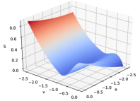
(a) $s_{\alpha}(v,e)$.

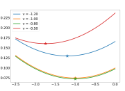
(b) $s_{\alpha}(v,e)$ as a function of $e$ with given value of $v$.

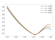
(c) $s_{\alpha}(v,e)$ as a function of $v$ with given value of $e$.

Figure 1: Landscape of $s_{\alpha}(v,e)$ based on (5) with $\alpha=0.05$ for the uniform distribution on $[-1,1]$.

Next, we provide the following theoretical guarantee for the well-behaved optimization landscape of the score function (5); also, see Figure 1 for a visualization.

Proposition 2.2.

(1) Assume ${\rm VaR}_{\alpha}(\mu)<0$, for $\alpha<1/2$. Then the score $s_{\alpha}(v,e)$ based on (5) is strictly consistent for $({\rm VaR}_{\alpha}(\mu),{\rm ES}_{\alpha}(\mu))$ and the Hessian of $s_{\alpha}(v,e)$ is positive semi-definite on the region

$$\mathcal{B}=\left\{(v,e)\,\,\left|\,\,v\leq{\rm VaR}_{\alpha}(\mu),\,\,\text{and}\,\,W_{\alpha}v\leq e\leq v\leq 0\right.\right\}.$$

(2) In addition, we assume there exist $\delta_{\alpha}\in(0,1)$, $\varepsilon_{\alpha}\in\left(0,\frac{1}{2}-\alpha\right)$, $z_{\alpha}\in\left(0,\frac{1}{2}-\alpha\right)$, and $W_{\alpha}>\frac{1}{\sqrt{\alpha}}$ such that

$$\frac{\mu(\mathrm{d}x)}{\mathrm{d}x}\geq\delta_{\alpha}\mbox{ for }x\in\left[{\rm VaR}_{\alpha}(\mu),{\rm VaR}_{\alpha+\varepsilon_{\alpha}}(\mu)\right]\quad{\rm and}\quad{\rm ES}_{\alpha}(\mu)\geq W_{\alpha}{\rm Var}_{\alpha}(\mu)+z_{\alpha}.$$ (6)

Then the Hessian of $s_{\alpha}(v,e)$ is positive semi-definite on the region

$$\widetilde{\mathcal{B}}=\left\{(v,e)\,\,\left|\,\,v\leq{\rm VaR}_{\alpha+\beta_{\alpha}}(\mu),\,\,\text{and}\,\,W_{\alpha}v+z_{\alpha}\leq e\leq v\leq 0\right.\right\}\quad{\rm where}\qquad\beta_{\alpha}=\min\left\{\varepsilon_{\alpha},\frac{z_{\alpha}\delta_{\alpha}}{2\,W_{\alpha}}\right\}.$$

See the proof of Proposition 2.2 in Appendix A.

Example 2.3 (Example for condition (6)).

Condition (6) holds when $X$ has a strictly positive density under measure $\mu$. Take an example where $X$ follows the standard normal distribution. Denote $f(x)=\frac{1}{\sqrt{2\pi}}\exp\left(-\frac{x^{2}}{2}\right)$ as the density function, and $F(y)=\int_{-\infty}^{y}f(x)\mathrm{d}x$ as the cumulative density function for $X$. Then we have ${\rm VaR}_{\alpha}(\mu)=F^{-1}(\alpha)$ and ${\rm ES}_{\alpha}(\mu)=-\frac{f(F^{-1}(\alpha))}{\alpha}$. Setting $\alpha=0.05$ and $\varepsilon_{\alpha}=0.05$, we have ${\rm VaR}_{0.05}(\mu)\approx-1.64$ and ${\rm ES}_{0.05}(\mu)\approx-2.06$ by direct calculation. Then we can set $\delta_{\alpha}=f(F^{-1}(0.05))\approx 0.103$, $W_{\alpha}=5$ and $z_{\alpha}=\frac{1}{4}$. Hence (6) holds for $\beta_{\alpha}=\min\{\varepsilon_{\alpha},\frac{z_{\alpha\delta_{\alpha}}}{2W_{\alpha}}\}\approx 0.0025$.

Proposition 2.2 implies that $s_{\alpha}(v,e)$ has a well-behaved optimization landscape on regions $\mathcal{B}$ and $\widetilde{\mathcal{B}}$ if the corresponding conditions are satisfied. In particular, the minimizer of $s_{\alpha}(v,e)$, i.e., $(\mbox{VaR}_{\alpha}(\mu),\mbox{ES}_{\alpha}(\mu))$, is on the boundary of region $\mathcal{B}$. $\widetilde{\mathcal{B}}$ contains an open ball with center $(\mbox{VaR}_{\alpha}(\mu),\mbox{ES}_{\alpha}(\mu))$.

In summary, $s_{\alpha}(v,e)$ has a positive semi-definite Hessian in a neighborhood of the minimum, which leads to desirable properties for convergence. There are other score functions with different choices of $H_{1}$ and $H_{2}$, but some of them may have undesirable properties (Fissler et al. [2016, 2015]) as the following example shows.

Example 2.4.

Let $X$ be uniformly distributed on $[-1,1]$ and $\alpha=0.05$. When $H_{2}(x)=\exp(x)$, there does not exist a constant $c<0$ such that

$$\frac{\partial s_{\alpha}^{2}}{\partial e^{2}}\geq 0\,\,\text{on}\,\,(-\infty,c].$$ (7)

(7) implies that the objective function $s_{\alpha}$ is not convex which renders the optimization problem difficult.

Proof of (7). If $X$ is uniformly distributed on $[-1,1]$ and $\alpha=0.05$, we have

$$\mu(X\leq v)v-\int_{-\infty}^{v}x\mu(x)+(e-v)\alpha=\frac{1}{4}v^{2}+\left(\frac{1}{2}-0.05\right)v+{\frac{1}{4}}+0.05e,$$

which yields

$$\frac{\partial^{2}s_{\alpha}}{\partial e^{2}}={\frac{\exp(e)}{\alpha}}\left[\frac{1}{4}(v+0.9)^{2}+0.0475+\alpha+0.05e\right].$$

Letting $v=-0.9$, we arrive at $\frac{\partial^{2}s_{\alpha}}{\partial e^{2}}|_{v=-0.9}<0$ for all $e<-1.95$.

The above analysis on the optimization landscapes for different score functions supports the choice of (5), as proposed by Acerbi and Szekely [2014] in our learning objective function (see next section).

3 Learning to generate tail scenarios

We now introduce the Tail Generative Adversarial Network (Tail-GAN) for simulating multivariate price scenarios. Given a set of input price scenarios as training data, Tail-GAN learns to simulate new price scenarios which lead to accurate tail risk statistics for a set of benchmark strategies, by solving a max-min game between a generator and a discriminator. The generator creates samples that are intended to approximate the tail distribution of the training data. The discriminator evaluates the quality of the simulated samples using tail risk measures, namely Value-at-Risk (VaR) and Expected Shortfall (ES), across a set of benchmark trading strategies, including static portfolios and dynamic trading strategies. Static portfolios and dynamic strategies capture properties of the price scenarios from different perspectives: static portfolios explore the correlation structure among the assets, while dynamic trading strategies, such as mean-reversion and trend-following strategies, discover temporal properties such as mean-reversion and trending properties. To train the generator and the discriminator, we use an objective function that leverages the elicitability of VaR and ES, and guarantees the consistency of the estimator.

3.1 Discriminator

Given measurable spaces $(X_{1},\Sigma_{1})$ and $(X_{2},\Sigma_{2})$, a measurable mapping $\Phi\colon X_{1}\to X_{2}$ and a measure $\mu\colon\Sigma_{1}\to[0,+\infty]$, the pushforward of $\mu$ is defined to be the measure $\Phi\#\mu$ given by, for any $B\in\Sigma_{2}$,

$$\Phi\#\mu(B)=\mu\Big{(}\Phi^{-1}(B)\Big{)}.$$ (8)

In addition, we consider $M$ assets and $K$ different trading strategies of interest. Denote $\mathbf{p}=\{(p_{m,t})_{t=1}^{T}\}_{m=1}^{M}$ as the matrix in $\mathbb{R}^{M\times T}$ that records the prices of each asset $m$, at the beginning of consecutive time intervals with duration $\Delta$. That is, each price scenario $\mathbf{p}$ contains the price information of $M$ assets over a total period of length $\Delta\times T$. Depending on the purpose of the simulator, $\Delta$ could range from milliseconds to minutes, and even to days. Each strategy is allocated the same initial capital, and trading decisions are made at discrete timestamps $t=1,2,\ldots,T$. In order for the strategies to be self-financed, there is no exogenous injection or withdrawal of capital. We consider $K$ benchmark strategies to discriminate the performance of the generator. For each strategy $k=1,2,\ldots,K$, a mapping $\Pi^{k}:\mathbb{R}^{M\times T}\rightarrow\mathbb{R}$ is defined to map the price scenarios $\mathbf{p}$ to the final PnL $x^{k}$ at terminal time $T$, that is, $\Pi^{k}(\mathbf{p})=x^{k}$. Finally, we use $\mathbf{\Pi}:=(\Pi^{1},\ldots,\Pi^{K})$ to define the mapping of all benchmark strategies.

Ideally, the discriminator $\overline{D}$ takes strategy PnL distributions as inputs, and outputs two values for each of the $K$ strategies, aiming to provide the correct $({\rm VaR}_{\alpha},{\rm ES}_{\alpha})$. Mathematically, this amounts to

$$\overline{D}^{*}\in\arg\min_{\overline{D}}\frac{1}{K}\sum_{k=1}^{K}\mathbb{E}_{\mathbf{p}\sim\mathbb{P}_{r}}\left[S_{\alpha}\left(\overbrace{\overline{D}(\underbrace{\Pi^{k}\#\mathbb{P}_{r}}_{\text{strategy PnL distribution}})}^{\text{VaR and ES prediction from }\overline{D}};\mathbf{p}\right)\right].$$ (9)

However, it is impossible to access the true distribution of $\mathbf{p}$, denoted as $\mathbb{P}_{r}$, in practice. Therefore we consider a sample-based version of the discriminator, which is easy to train in practice. To this end, we consider PnL samples $\{\mathbf{p}_{i}\}_{i=1}^{n}$ with a fixed size $n$ as the input of the discriminator. Mathematically, we write

$${D}^{*}\in\arg\min_{{D}}\frac{1}{K}\sum_{k=1}^{K}\frac{1}{n}\sum_{i=1}^{n}\left[S_{\alpha}\left(\overbrace{{D}(\underbrace{\Pi^{k}(\mathbf{p}_{j}),j\in[n]}_{\text{strategy PnL samples}})}^{\text{VaR and ES prediction from }D};\mathbf{p}_{i}\right)\right].$$ (10)

Here the expectation in (9) is replaced by the empirical mean using finite samples $\{\mathbf{p}_{i}\}_{i=1}^{n}$. In (10), we search the discriminator $D$ over all Lipschitz functions parameterized by the neural network architecture. Specifically, the discriminator adopts a neural network architecture with $\tilde{L}$ layers, and the input dimension is $\tilde{n}_{1}:=n$ and the output dimension is $\tilde{n}_{\tilde{L}}:=2$. Note that the $\alpha$-VaR of a distribution can be approximated by the $\lfloor\alpha n\rfloor{}^{th}$ smallest value in a sample of size $n$ from this distribution, which is permutation-invariant to the ordering of the samples. Given that the goal of the discriminator is to predict the $\alpha$-VaR and $\alpha$-ES, including a sorting function in our architecture design could potentially improve the stability of the discriminator. We denote this (differentiable) neural sorting function as $\widetilde{\Gamma}$ (Grover et al. [2019]), with details deferred to Appendix B.3.

In summary, the discriminator is given by

$$D(\mathbf{x}^{k};\mathbf{\delta})=\widetilde{\mathbf{W}}_{\tilde{L}}\cdot\sigma\left(\widetilde{\mathbf{W}}_{\tilde{L}-1}\ldots\sigma(\widetilde{\mathbf{W}}_{1}{\widetilde{\Gamma}(\mathbf{x}^{k})}+\widetilde{\mathbf{b}}_{1})\ldots+\widetilde{\mathbf{b}}_{\tilde{L}-1}\right)+\widetilde{\mathbf{b}}_{\tilde{L}},$$ (11)

where $\mathbf{\delta}=(\widetilde{\mathbf{W}},\widetilde{\mathbf{b}})$ represent all the parameters in the neural network. Here we have $\widetilde{\mathbf{W}}=(\widetilde{\mathbf{W}}_{1},\widetilde{\mathbf{W}}_{2},\ldots,\widetilde{\mathbf{W}}_{\tilde{L}})$ and $\widetilde{\mathbf{b}}=(\widetilde{\mathbf{b}}_{1},\widetilde{\mathbf{b}}_{2},\ldots,\widetilde{\mathbf{b}}_{\tilde{L}})$ with $\widetilde{\mathbf{W}}_{l}\in\mathbb{R}^{n_{l}\times n_{l-1}}$, $\widetilde{\mathbf{b}}_{l}\in\mathbb{R}^{n_{l}\times 1}$ for $l=1,2,\ldots,\tilde{L}$. In the neural network literature, the $\widetilde{\mathbf{W}}_{l}$’s are often called the weight matrices, the $\widetilde{\mathbf{b}}_{l}$’s are called bias vectors. The outputs of the discriminator are two values for each of the $K$ strategies, (hopefully) representing the $\alpha$-VaR and $\alpha$-ES. The operator $\sigma(\cdot)$ takes a vector of any dimension as input, and applies a function component-wise. $\sigma(\cdot)$ is referred to as the activation function. Specifically, for any $q\in\mathbb{Z}^{+}$ and any vector $\mathbf{u}=(u_{1},u_{2},\ldots,u_{q})^{\top}\in\mathbb{R}^{q}$, we have that $\sigma(\mathbf{u})=(\sigma(u_{1}),\sigma(u_{2}),\ldots,\sigma(u_{q}))^{\top}.$ Several popular choices for the activation function include ReLU with $\sigma(u)=\max(u,0)$, Leaky ReLU with $\sigma(u)=a_{1}\,\max(u,0)-a_{2}\,\max(-u,0)$ and $a_{1},a_{2}>0$, and smooth functions such as $\sigma(\cdot)=\tanh(\cdot)$. We sometimes use the abbreviation $D_{\mathbf{\delta}}$ or $D$ instead of $D(\cdot;\mathbf{\delta})$ for notation simplicity.

Accordingly, we define $\mathcal{D}$ as a class of discriminators

$$\mathcal{D}(\tilde{L},\tilde{n}_{1},\ldots,\tilde{n}_{\tilde{L}}) = \Big{\{}D:\mathbb{R}^{n}\rightarrow\mathbb{R}^{2}\,\,\Big{|}\,\,D\mbox{ takes the form in }\eqref{eq:discriminator}\mbox{ with }\tilde{L}\mbox{ layers and }\tilde{n}_{l}\mbox{ as the }$$ (12)

$$\quad\mbox{ width of each layer},\|\widetilde{\mathbf{W}}_{l}\|_{\infty},\|\widetilde{\mathbf{b}}_{l}\|_{\infty}<\infty\mbox{ for }l=1,2,\ldots,\tilde{L}\Big{\}},$$

where $\|\cdot\|_{\infty}$ denotes the max-norm that takes the max absolute value of all elements in the input matrix or vector.

3.2 Generator

For the generator, we use a neural network with $L\in\mathbb{Z}^{+}$ layers. Denoting by $n_{l}$ the width of the $l$-th layer, the functional form of the generator is given by

$$G(\mathbf{z};\mathbf{\gamma})=\mathbf{W}_{L}\cdot\sigma\left(\mathbf{W}_{L-1}\ldots\sigma(\mathbf{W}_{1}\mathbf{z}+\mathbf{b}_{1})\ldots+\mathbf{b}_{L-1}\right)+\mathbf{b}_{L},$$ (13)

in which $\mathbf{\gamma}:=(\mathbf{W},\mathbf{b})$ represents the parameters in the neural network, with $\mathbf{W}=(\mathbf{W}_{1},\mathbf{W}_{2},\ldots,\mathbf{W}_{L})$ and $\mathbf{b}=(\mathbf{b}_{1},\mathbf{b}_{2},\ldots,\mathbf{b}_{L})$. Here $\mathbf{W}_{l}\in\mathbb{R}^{n_{l}\times n_{l-1}}$ and $\mathbf{b}_{l}\in\mathbb{R}^{n_{l}\times 1}$ for $l=1,2,\ldots,L$, where $n_{0}=N_{z}$ is the dimension of the input variable.

We define $\mathcal{G}$ as a class of generators that satisfy given regularity conditions on the neural network parameters

$$\mathcal{G}(L,n_{1},n_{2},\ldots,n_{L}) = \Big{\{}G:\mathbb{R}^{N_{z}}\rightarrow\mathbb{R}^{M\times T}\,\,\Big{|}\,\,G\mbox{ takes the form in }\eqref{eq:generator}\mbox{ with }L\mbox{ layers and }n_{l}\mbox{ as the }$$ (14)

$$\quad\mbox{ width of each layer},\|\mathbf{W}_{l}\|_{\infty},\|\mathbf{b}_{l}\|_{\infty}<\infty\mbox{ for }l=1,2,\ldots,L\Big{\}}.$$

To ease the notation, we may use the abbreviation $G_{\mathbf{\gamma}}(\cdot)$ or drop the dependency of $G(\cdot\,;\mathbf{\gamma})$ on the neural network parameters $\mathbf{\gamma}$ and conveniently write $G(\cdot)$. We further denote $\mathbb{P}_{G}$ as the distribution of price series generated by $G$ under the initial distribution $\mathbf{z}\sim\mathbb{P}_{\mathbf{z}}$.

Universal approximation property of the generator.

We first demonstrate the universal approximation power of the generator under the VaR and ES criteria, and then we provide a similar result for more general risk measures that satisfy certain Hölder regularity property.

Given two probability measures $\mu$ and $\nu$ on $\mathbb{R}^{d}$, recall in (8) that a transport map $\Phi$ between $\mu$ and $\nu$ is a measurable map $\Phi:\mathbb{R}^{d}\rightarrow\mathbb{R}^{d}$ such that $\nu=\Phi\#\mu$. We denote by $\Gamma(\mu,\nu)$ the set of transport plans between $\mu$ and $\nu$ which consists of all coupling measures $\gamma$ of $\mu$ and $\nu$, i.e., $\gamma(A\times\mathbb{R}^{d})=\mu(A)$ and $\gamma(\mathbb{R}^{d}\times B)=\gamma(B)$ for any measurable $A,B\subset\mathbb{R}^{d}$ .

We assume that the portfolio values are Lipschitz-continuous with respect to price paths:

Assumption 3.1 (Lipschitz Continuity of the Portfolio Value).

For $k=1,2,\cdots,K$,

$$\exists\ell_{k}>0,\qquad|\Pi^{k}(x)-\Pi^{k}(y)|\leq\ell_{k}\|x-y\|,\quad\forall x,y\in\mathbb{R}^{{}^{M\times T}}.$$

Recall $\mathbb{P}_{r}$ and $\mathbb{P}_{z}$ are respectively the target distribution and the distribution of the input noise.

Assumption 3.2 (Noise Distribution and Target Distribution).

$\mathbb{P}_{r}$ and $\mathbb{P}_{z}$ are probability measures on $\mathbb{R}^{M\times T}$ (i.e. $N_{z}=M\times T$) satisfying the following conditions:

• $\mathbb{P}_{z}\in\mathcal{P}^{2}(\mathbb{R}^{M\times T})$ is absolutely continuous with respect to the Lebesgue measure.

• $\mathbb{P}_{r}$ has a bounded moment of order $\beta>1$: $\int\|x\|^{\beta}\mathbb{P}_{r}(dx)<\infty$,.

Theorem 3.3 (Universal Approximation under VaR and ES Criteria).

Under Assumptions 3.1-3.2 and the additional assumption

• The random variables $\Pi^{k}(X)$ have continuous densities $f_{k}$ under $\mathbb{P}_{r}$ and there exist $\eta_{k},\delta_{k}>0$ such that $f_{k}(x)>\eta_{k}$ for all $x\in[{\rm VaR}_{\alpha}(\Pi^{k}\#\mathbb{P}_{r})-\frac{\delta_{k}}{2},{\rm VaR}_{\alpha}(\Pi^{k}\#\mathbb{P}_{r})+\frac{\delta_{k}}{2}]$.

we have, for any $\varepsilon>0$

• there exists a positive integer $n_{1}=\mathcal{O}(\varepsilon^{-2})$, and a feed-forward neural network $G_{1}$ with $L=\lceil\log n_{1}\rceil$ fully connected layers of equal width $N=2^{L}$ and ReLU activation, such that

  $$\Big{|}{\rm VaR}_{\alpha}\Big{(}\Pi^{k}\#\Big{(}(\nabla G_{1})\#\mathbb{P}_{z}\Big{)}\Big{)}-{\rm VaR}_{\alpha}\Big{(}\Pi^{k}\#\mathbb{P}_{r}\Big{)}\Big{|}<\varepsilon;$$

• there exists a positive integer $n_{2}=\mathcal{O}(\varepsilon^{-\frac{\beta}{\beta-1}})$, and a feed-forward neural network $G_{2}$ with $L=\lceil\log n_{2}\rceil$ fully connected layers of equal width $N=2^{L}$ and ReLU activation, such that

  $$\Big{|}{\rm ES}_{\alpha}\Big{(}\Pi^{k}\#\Big{(}(\nabla G_{2})\#\mathbb{P}_{z}\Big{)}\Big{)}-{\rm ES}_{\alpha}\Big{(}\Pi^{k}\#\mathbb{P}_{r}\Big{)}\Big{|}<\varepsilon.$$

Theorem 3.3 implies that a feed-forward neural network with fully connected layers of equal-width neural network is capable of generating scenarios which reproduce the tail risk properties (VaR and ES) for the benchmark strategies with arbitrary accuracy. This justifies the use of this simple network architecture for Tail-GAN. The size of the network, namely the width and the length, depends on the tolerance of the error $\varepsilon$ and depends on $\beta$ in the case of ES.

The proof (given in Appendix A) consists in using the theory of (semi-discrete) optimal transport to build a transport map of the form $\Phi=\nabla\psi$ which pushes the source distribution $\mathbb{P}_{z}$ to the empirical distribution $\mathbb{P}_{r}^{(n)}$. The potential $\psi$ has an explicit form in terms of the maximum of finitely many affine functions. Such an explicit structure enables the representation of $\psi$ with a finite deep neural network [Lu and Lu 2020].

We now provide a universal approximation result for more general law-invariant risk measures. Consider a risk measure, defined as a map $\rho:\mathcal{L}\rightarrow\mathbb{R}$ on the set $\mathcal{L}$ of probability measures on $\mathbb{R}$. VaR, ES, and spectral risk measures are examples of such risk measures (Cont et al. [2013]). With a slight abuse of notation, for a real-valued random variable $X$ with CDF $F$, we will write $\rho(X)=\rho(F)$.

Denote by

$$\mathcal{W}_{p}(\mu,\nu)=\inf_{\xi\in\mathcal{C}(\mu,\nu)}\Big{[}\mathbb{E}_{(X,Y)\sim\xi}\|X-Y\|^{p}\Big{]}^{1/p},$$

the Wasserstein distance of order $p\in[1,\infty)$ between two probability measures $\mu$ and $\nu$ on $\mathbb{R}^{d}$, where $\mathcal{C}(\mu,\nu)$ denotes the collection of all distributions on $\mathbb{R}^{d}\times\mathbb{R}^{d}$ with marginal distributions $\mu$ and $\nu$.

Theorem 3.4 (Universal Approximation under General Risk Measure).

Under Assumptions 3.1-3.2 and the additional assumption that

• $\rho$ is Hölder continuous for the Wasserstein-1 metric:

  $$\exists L>0,\quad\exists\kappa\in(0,1],\quad\Big{|}\rho(\Pi^{k}\#\mu)-\rho(\Pi^{k}\#\nu))\Big{|}\leq L\Big{(}\,\mathcal{W}_{1}\Big{(}\Pi^{k}\#\mu,\Pi^{k}\#\nu\Big{)}\,\Big{)}^{\kappa},$$ (15)

for any $\varepsilon$, there exists a positive integer $n_{3}$, and a feed-forward neural network $G_{3}$ with $L=\lceil\log n_{3}\rceil$ fully connected layers with equal width $N=2^{L}$ and ReLU activation such that

$$\Big{|}\,\rho\Big{(}\Pi^{k}\#\Big{(}\nabla G_{3}{\#}\mathbb{P}_{z}\Big{)}\Big{)}-\rho\Big{(}\Pi^{k}\#\mathbb{P}_{r}\Big{)}\,\Big{|}<\varepsilon.$$

Furthermore,

1. $n_{3}=\mathcal{O}\left(\varepsilon^{-\frac{\beta}{\kappa(\beta-1)}}\right)$ when $M=T=1$ and $1<\beta\leq 2$;

2. $n_{3}=\mathcal{O}\left(\varepsilon^{-\frac{2}{\kappa}}\right)$ when $M=T=1$ and $\beta\geq 2$;

3. $n_{3}=\mathcal{O}\left(\varepsilon^{-\frac{M\times T}{\kappa}}\right)$ when $M\times T\geq 2$ and $\frac{1}{M\times T}+\frac{1}{\beta}<1$;

4. $n_{3}=\mathcal{O}\left(\varepsilon^{-\frac{\beta}{\kappa(\beta-1)}}\right)$ when $M\times T\geq 2$ and $\frac{1}{M\times T}+\frac{1}{\beta}\geq 1$.

Remark 3.5.

Examples of risk measures that are Hölder continuous, i.e. which satisfy Assumption A4 are the optimized certainty equivalent (Ben-Tal and Teboulle [1986, 2007]), spectral risk measures (Acerbi [2002]), and utility-based shortfall risk (Föllmer and Schied [2002]).

As suggested in Theorem 3.4, the depth of the neural network depends on $\beta$, $M\times T$, and $\kappa$. $M=K=1$ corresponds to the simulation of a single price value of a single asset, which is not much of an interesting case. When $M\times T\geq 2$ and $\beta>\frac{M\times T}{M\times T-1}$, the complexity of the neural network, characterized by $n_{3}$, depends on the ratio between the dimension of the price scenario $M\times T$ and the Lipschitz exponent $\kappa$. When $\mathbb{P}_{r}$ is heavy-tailed in the sense that $1<\beta<\frac{M\times T}{M\times T-1}$, $n_{3}$ is determined by $\frac{\beta}{(\beta-1)\kappa}$. The proof of Theorem 3.4 is deferred to Appendix A.

3.3 Loss function

We now design a loss function to train both the generator and the discriminator together. We start with a bi-level optimization formulation and then introduce the max-min game formulation by relaxing the lower-level optimization problem. We also show that these two formulations are equivalent under mild conditions.

Bi-level optimization problem.

We first start with a theoretical version of the objective function to introduce some insights and then provide the practical sample-based version for training. Given two classes of functions $\overline{\mathcal{G}}:=\{\overline{G}\,:\,\mathbb{R}^{N_{z}}\rightarrow\mathbb{R}^{M\times T}\}$ and $\overline{\mathcal{D}}:=\{\overline{D}\,:\,\mathcal{P}(\mathbb{R})\rightarrow\mathbb{R}^{2}\}$, our goal is to find a generator $\overline{G}^{*}\in\overline{\mathcal{G}}$ and a discriminator $\overline{D}^{*}\in\overline{\mathcal{D}}$ via the following bi-level (or constrained) optimization problem

$$\overline{G}^{*}\in\arg\min_{\overline{G}\in\overline{\mathcal{G}}}\frac{1}{K}\,\sum_{k=1}^{K}\mathbb{E}_{\mathbf{p}\sim\mathbb{P}_{r}}\left[S_{\alpha}\Big{(}\overline{D}^{*}\big{(}\Pi^{k}\#\mathbb{P}_{\overline{G}}\big{)},\,\,\Pi^{k}(\mathbf{p})\Big{)}\right],$$ (16)

where $\mathbb{P}_{\overline{G}}\in\mathcal{P}(\mathbb{R}^{M\times T})$ is the distribution of the samples from $\overline{G}$ and

$$\overline{D}^{*}\in\arg\min_{\overline{D}\in\overline{\mathcal{D}}}\frac{1}{K}\,\sum_{k=1}^{K}\mathbb{E}_{\mathbf{p}\sim\mathbb{P}_{r}}\left[S_{\alpha}\Big{(}\overline{D}\big{(}\Pi^{k}\#\mathbb{P}_{r}\big{)},\,\,\Pi^{k}(\mathbf{p})\Big{)}\right].$$ (17)

In the bi-level optimization problem (16)-(17), the discriminator $\overline{D}^{*}$ aims to map the PnL distribution $\Pi^{k}\#\mathbb{P}_{r}$ to the associated $\alpha$-VaR and $\alpha$-ES values. Given the definition of the score function and the joint elicitability property of VaR and ES, we have $\overline{D}^{*}(\cdot):=({\rm VaR}_{\alpha},{\rm ES}_{\alpha})(\cdot)$ according to (3). Assume $\overline{D}^{*}$ solves (17), the simulator $\overline{G}^{*}\in\overline{\mathcal{G}}$ in (16) aims to map the noise input to a price scenario that has consistent ${\rm VaR}$ and ${\rm ES}$ values of the strategy PnLs applied to $\mathbb{P}_{r}$. Note our current formulation (16)-(17) implicitly assumes that the user of our Tail-GAN framework assigns equal importance to the losses of all trading strategies of interest. It can be adapted to account for different weights if some of the strategies are more important than others.

From bi-level optimization to max-min game.

In practice, constrained optimization problems are difficult to solve, and one can instead relax the constraint by applying the Lagrangian relaxation method with a dual parameter $\lambda>0$, leading to a max-min game between two neural networks $\overline{D}$ and $\overline{G}$,

$$\max_{\overline{D}\in\overline{\mathcal{D}}_{0}}\min_{\overline{G}\in\overline{\mathcal{G}}}\frac{1}{K}\,\sum_{k=1}^{K}\Bigg{[}\mathbb{E}_{\mathbf{p}\sim\mathbb{P}_{r}}\left[\,\,S_{\alpha}\Big{(}\overline{D}\big{(}\Pi^{k}\#\mathbb{P}_{\overline{G}}\big{)},\Pi^{k}(\mathbf{p})\Big{)}\right]-\lambda\,\,\mathbb{E}_{\mathbf{p}\sim\mathbb{P}_{r}}\left[S_{\alpha}\Big{(}\overline{D}(\Pi^{k}\#\mathbb{P}_{r}),\,\,\Pi^{k}(\mathbf{p})\Big{)}\right]\,\,\Bigg{]},$$ (18)

where

$$\overline{\mathcal{D}}_{0}:=\Big{\{}\overline{D}\,: \mathcal{P}^{1}(\mathbb{R})\rightarrow\mathbb{R}^{2}\,\,\textit{ and }\,\,\exists\mu\in\mathcal{P}(\mathbb{R}^{M\times T})\text{ with a finite first moment }\,\,\text{s.t.}$$ (19)

$$\overline{D}(\Pi^{k}\#\mu)=({\rm VaR}_{\alpha}(\Pi^{k}\#\mathbb{P}_{r}),{\rm ES}_{\alpha}(\Pi^{k}\#\mathbb{P}_{r})),k=1,2,\cdots,K\,\Big{\}}$$

is a smaller set of discriminators such that $\overline{\mathcal{D}}_{0}\subseteq\mathcal{D}$. Note that the condition in (19) implies that $\overline{D}$ is sensitive to the input distribution, leading to a non-degenerate mapping. This is not a restrictive condition to impose. Intuitively, if the discriminator detects that the samples come from the true distribution, it will provide a pair of values that is close to the minimizer of the score function, namely the VaR and ES values of the true distribution, in accordance with the elicitability property.

Theorem 3.6 (Equivalence of the Formulations).

Set $N_{z}=M\times T$. Assume that $\mathbb{P}_{z}$ has a finite first moment and is absolutely continuous with respect to the Lebesgue measure. Then the max-min game (18) with $\overline{\mathcal{D}}_{0}$ is equivalent to the bi-level optimization problem (16)-(17) for any $\lambda>0$.

The proof of Theorem 3.6 is deferred to Appendix A.

A sample-based version of the loss function.

As we explained in Section 3.1, it is impossible to access the true distribution $\mathbb{P}_{r}$ in practice. Therefore we consider a sample-based version of the discriminator, which is easy to train in practice. This leads to the following formulation of the loss function

$\displaystyle\max_{D\in\mathcal{D}}\min_{G\in\mathcal{G}}\frac{1}{Kn}\,\sum_{k=1}^{K}\sum_{j=1}^{n}\Big{[}S_{\alpha}\Big{(}D\big{(}\Pi^{k}(\mathbf{q}_{i});i\in[n]\big{)},\Pi^{k}(\mathbf{p}_{j})\Big{)}-\lambda\,\,S_{\alpha}\Big{(}D(\Pi^{k}(\mathbf{p}_{i});i\in[n]),\,\,\Pi^{k}(\mathbf{p}_{j})\Big{)}\Big{]}$ (20)

where $\mathbf{p}_{i},\mathbf{p}_{j}\sim\mathbb{P}_{r}$ and $\mathbf{q}_{i}\sim\mathbb{P}_{G}$ ($i,j=1,2,\ldots,n$). The discriminator $D$ takes $n$ PnL samples as the input and aims to provide the VaR and ES values of the sample distribution as the output. (See Section 3.1 for the design of the discriminator.) The score function $S_{\alpha}$ is defined in (5). In addition, the max-min structure of (18) encourages the exploration of the generator to simulate scenarios that are not exactly the same as what is observed in the input price scenarios, but are equivalent under the criterion of the score function, hence improving generalization. We refer the readers to Section 5.3 for a comparison between Tail-GAN and supervised learning methods and a demonstration of the generalization power of Tail-GAN.

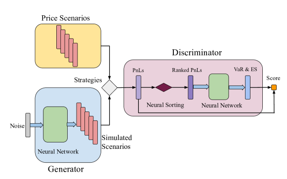
Figure 2: Architecture of Tail-GAN. The (blue) thick arrows represent calculations with learnable parameters, and the (black) thin arrows represent calculations with fixed parameters.

Compared to the Jensen-Shannon divergence used in the loss function of standard GAN architectures (Goodfellow et al. [2014]) and Wasserstein distance in WGAN (Arjovsky et al. [2017]), the objective function in (18) with the score function $S_{\alpha}$ is more sensitive to tail risk and leads to an output which better approximates the $\alpha$-ES and $\alpha$-VaR values. The architecture of Tail-GAN is depicted in Figure 2.

4 Numerical experiments: methodology and performance evaluation

Before we proceed with the numerical experiments on both synthetic data sets and real financial data sets, we first describe the methodologies, performance evaluation criterion, and several baseline models for comparison.

4.1 Methodology

Algorithm 1 provides a detailed description of the training procedure of Tail-GAN, which allows us to train the simulator with different benchmark trading strategies.

Algorithm 1 Tail-GAN.

Input:
$\bullet$ Price scenarios $\mathbf{p}_{1},\dots,\mathbf{p}_{N}\in\mathbb{R}^{M\times T}$.
$\bullet$ Description of trading strategies: $\mathbf{\Pi}=(\Pi^{1},\dots,\Pi^{K}):\mathbb{R}^{M\times T}\to\mathbb{R}^{K}$.
$\bullet$ Hyperparameters: learning rate $l_{D}$ for discriminator and $l_{G}$ for generator; number of training epochs; batch size $N_{B}$; dual parameter $\lambda$.

1:for number of epochs do

2:     for $j=1\to\lfloor N/N_{B}\rfloor$ do

3:         Generate $N_{B}$ IID noise samples $\{\mathbf{z}_{i},i\in[N_{B}]\}\sim\mathbb{P}_{\mathbf{z}}$.

4:         Sample a batch $\mathcal{B}_{j}\subset\{1,\dots,N\}$ of size $N_{B}$ from the input data $\{\mathbf{p}_{i},i=1,\dots,N\}$.

5:         Compute the loss of the discriminator on the batch $\mathcal{B}_{j}$

$$\mathcal{L}_{D}(\mathbf{\delta})=\frac{1}{K\,N_{B}}\,\,\sum_{k=1}^{K}\sum_{n\in\mathcal{B}_{j}} \Big{[}S_{\alpha}\big{(}D_{{\mathbf{\delta}}}(\Pi^{k}(G_{{\mathbf{\gamma}}}({\mathbf{z}_{i}})),i\in[N_{B}]),\Pi^{k}(\mathbf{p}_{n})\big{)}$$

$$-\lambda S_{\alpha}\big{(}D_{{\mathbf{\delta}}}(\Pi^{k}(\mathbf{p}_{i}),i\in\mathcal{B}_{j}),\Pi^{k}(\mathbf{p}_{n})\big{)}\Big{]}.$$

6:         Update the discriminator

$$\mathbf{\delta}\leftarrow\mathbf{\delta}+l_{D}\nabla\mathcal{L}_{D}(\mathbf{\delta}).$$

7:         Generate $N_{B}$ IID noise samples $\{\tilde{\mathbf{z}}_{i},i\in[N_{B}]\}\sim\mathbb{P}_{\mathbf{z}}$.

8:         Compute the loss of the generator

$$\mathcal{L}_{G}(\mathbf{\gamma})=\frac{1}{K\,N_{B}}\,\,\sum_{k=1}^{K}\sum_{n\in\mathcal{B}_{j}}S_{\alpha}\big{(}D_{{\delta}}(\Pi^{k}(G_{{\mathbf{\gamma}}}({\tilde{\mathbf{z}}_{i}})),i\in[N_{B}]),\Pi^{k}(\mathbf{p}_{n})\big{)}.$$

9:         Update the generator

$$\mathbf{\gamma}\leftarrow\mathbf{\gamma}-l_{G}\nabla\mathcal{L}_{G}(\mathbf{\gamma}).$$

10:     end for

11:end for

12:$\mathbf{\gamma}^{*}=\mathbf{\gamma},\qquad\mathbf{\delta}^{*}=\mathbf{\delta}$.

Outputs:
$\bullet$ $\mathbf{\delta}^{*}$: trained discriminator weights;  $\mathbf{\gamma}^{*}$: trained generator weights.
$\bullet$ Simulated scenarios: $G_{\mathbf{\gamma}^{*}}(\mathbf{z}_{i})$ where $\mathbf{z}_{i}\sim\mathbb{P}_{\mathbf{z}}$ IID.

For ease of exposition, unless otherwise stated, we denote Tail-GAN as the model (introduced in Section 3) trained with both static and dynamic trading strategies across multiple assets, as this is a typical set-up used by asset managers. We compare Tail-GAN with four benchmark models:

• Tail-GAN-Raw: Tail-GAN trained (only) with (static) buy-and-hold strategies on individual asset.

• Tail-GAN-Static: Tail-GAN trained (only) with static multi-asset portfolios.

• Historical Simulation Method (HSM): Using VaR and ES computed from historical data as the prediction for VaR and ES of future data.

• Wasserstein GAN (WGAN): trained on asset return data with Wasserstein distance as the loss function. We refer to Arjovsky et al. [2017] for more details on WGAN.

As Tail-GAN-Raw is trained with the PnLs of single-asset portfolios, it shares the same spirit as Quant-GAN (Wiese et al. [2020]) as well as many GAN-based generators for financial time series (such as Koshiyama et al. [2020], Marti [2020], Ni et al. [2020], Takahashi et al. [2019], Li et al. [2020]). Tail-GAN-Static is trained with the PnLs of multi-asset portfolios which is more flexible than Tail-GAN-Raw by allowing different capital allocations among different assets. This could potentially capture the correlation patterns among different assets. In addition to the static portfolios, Tail-GAN also includes dynamic strategies to capture temporal dependence information in financial time series.

4.2 Performance evaluation criteria

We introduce the following criteria to compare the scenarios simulated using Tail-GAN with other simulation models: (1) tail behavior comparison; (2) structural characterizations such as correlation and auto-correlation; and (3) model verification via (statistical) hypothesis testing such as the Score-based Test and Coverage Test. The first two evaluation criteria are applied throughout the numerical analysis for both synthetic and real financial data, while the hypothesis tests are only for synthetic data as they require the knowledge of “oracle” estimates of the true data generating process.

Tail behavior.

To evaluate how closely the VaR (ES) of strategy PnLs, computed under the generated scenarios, match the ground-truth VaR (ES) of the strategy PnLs computed under input scenarios, we employ both quantitative and qualitative assessment methods to gain a thorough understanding.

The quantitative performance measure is relative error of VaR and ES. For any strategy $k$ $(1\leq k\leq K)$, the relative error of VaR is defined as $\frac{\left|{\rm VaR}_{\alpha}\left(\Pi^{k}\#\mathbb{P}_{G}^{(\mathfrak{N})}\right)-{\rm VaR}_{\alpha}\left(\Pi^{k}\#\mathbb{P}_{r}\right)\right|}{\left|{\rm VaR}_{\alpha}\left(\Pi^{k}\#\mathbb{P}_{r}\right)\right|}$, where ${\rm VaR}_{\alpha}\left(\Pi^{k}\#\mathbb{P}_{r}\right)$ is the $\alpha$-VaR of the PnL for strategy $k$ evaluated under $\mathbb{P}_{r}$ and ${\rm VaR}_{\alpha}\left(\Pi^{k}\#\mathbb{P}_{G}^{(\mathfrak{N})}\right)$ is the empirical estimate of VaR for strategy $k$ evaluated with $\mathfrak{N}$ samples under $\mathbb{P}_{G}$. Similarly, for the estimates ${\rm ES}_{\alpha}\left(\Pi^{k}\#\mathbb{P}_{G}^{(\mathfrak{N})}\right)$, we define the relative error as $\frac{\left|{\rm ES}_{\alpha}\left(\Pi^{k}\#\mathbb{P}_{G}^{(\mathfrak{N})}\right)-{\rm ES}_{\alpha}\left(\Pi^{k}\#\mathbb{P}_{r}\right)\right|}{\left|{\rm ES}_{\alpha}\left(\Pi^{k}\#\mathbb{P}_{r}\right)\right|}$ for the ES of strategy $k$. We then use the following average relative errors of VaR and ES as the overall measure of model performance

$${\rm RE}(\mathfrak{N})=\frac{1}{2K}\sum_{k=1}^{K}\left(\frac{\left|{\rm VaR}_{\alpha}\left(\Pi^{k}\#\mathbb{P}_{G}^{(\mathfrak{N})}\right)-{\rm VaR}_{\alpha}\left(\Pi^{k}\#\mathbb{P}_{r}\right)\right|}{\left|{\rm VaR}_{\alpha}\left(\Pi^{k}\#\mathbb{P}_{r}\right)\right|}+\frac{\left|{\rm ES}_{\alpha}\left(\Pi^{k}\#\mathbb{P}_{G}^{(\mathfrak{N})}\right)-{\rm ES}_{\alpha}\left(\Pi^{k}\#\mathbb{P}_{r}\right)\right|}{\left|{\rm ES}_{\alpha}\left(\Pi^{k}\#\mathbb{P}_{r}\right)\right|}\right).$$

One useful benchmark is to compare the above relative error with the sampling error bellow, when only using a finite number of real samples to calculate VaR and ES

$${\rm SE}(\mathfrak{N})=\frac{1}{2K}\sum_{k=1}^{K}\left(\frac{\left|{\rm VaR}_{\alpha}\left(\Pi^{k}\#\mathbb{P}_{r}^{(\mathfrak{N})}\right)-{\rm VaR}_{\alpha}\left(\Pi^{k}\#\mathbb{P}_{r}\right)\right|}{\left|{\rm VaR}_{\alpha}\left(\Pi^{k}\#\mathbb{P}_{r}\right)\right|}+\frac{\left|{\rm ES}_{\alpha}\left(\Pi^{k}\#\mathbb{P}_{r}^{(\mathfrak{N})}\right)-{\rm ES}_{\alpha}\left(\Pi^{k}\#\mathbb{P}_{r}\right)\right|}{\left|{\rm ES}_{\alpha}\left(\Pi^{k}\#\mathbb{P}_{r}\right)\right|}\right),$$

where ${\rm VaR}_{\alpha}\left(\Pi^{k}\#\mathbb{P}_{r}^{(\mathfrak{N})}\right)$ and ${\rm ES}_{\alpha}\left(\Pi^{k}\#\mathbb{P}_{r}^{(\mathfrak{N})}\right)$ are the estimates for VaR and ES of strategy $k$ using ground-truth data with sample size $\mathfrak{N}$.

GANs are usually trained with a finite number of samples, and thus it is difficult for the trained GAN to achieve a better sampling error of the training data with the same sample size. To this end, we may conclude that the trained GAN reaches its best finite-sample performance if ${\rm RE}(\mathfrak{N})$ is comparable to ${\rm SE}(\mathfrak{N})$. This benchmark comparison and model validation steps are important to evaluate the performance of GAN models. However, these steps are missing in the GAN literature for simulating financial time series (Wiese et al. [2020]).

We also use rank-frequency distribution to visualize the tail behaviors of the simulated data versus the market data. Rank-frequency distribution is a discrete form of the quantile function, i.e., the inverse cumulative distribution, giving the size of the element at a given rank. By comparing the rank-frequency distribution of the market data and simulated data of different strategies, we gain an understanding of how good the simulated data is in terms of the risk measures of different strategies.

Structural characterization.

We are interested in testing whether Tail-GAN is capable of capturing structural properties, such as temporal and spatial correlations, of the input price scenarios. To do so, we calculate and compare the following statistics of the output price scenarios generated by each simulator: (1) the sum of the absolute difference between the correlation coefficients of the input price scenario and those of generated price scenario, and (2) the sum of the absolute difference between the autocorrelation coefficients (up to 10 lags) of the input price scenario and those of the generated price scenario.

Hypothesis testing for synthetic data.

Given the benchmark strategies and a simulation model (generically referred to as $\mathcal{M}$), we are interested in testing (or rejecting) whether risk measures for benchmark strategies estimated from simulated scenarios $\mathcal{M}$ are as accurate as “oracle” estimates given knowledge of the true data generating process. Here, $\mathcal{M}$ may represent Tail-GAN, Tail-GAN-Raw, Tail-GAN-Static, HSM, and WGAN.

We explore two methods, the Score-based Test and the Coverage Test, to verify the relationship between the simulator $\mathcal{M}$ and the true model. We first introduce the Score-based Test to verify the hypothesis

$$\mathcal{H}_{0}: \mathbb{E}_{\mathbf{p}\sim\mathbb{P}_{r}}\left[S_{\alpha}\big{(}{\rm VaR}_{\alpha}\left(\Pi^{k}\#\mathbb{P}_{\mathcal{M}}\right),{\rm ES}_{\alpha}\left(\Pi^{k}\#\mathbb{P}_{\mathcal{M}}\right),{\Pi^{k}(\mathbf{p})}\big{)}\right]$$

$$=\mathbb{E}_{\mathbf{p}\sim\mathbb{P}_{r}}\left[S_{\alpha}\big{(}{\rm VaR}_{\alpha}\left(\Pi^{k}\#\mathbb{P}_{r}\right),{\rm ES}_{\alpha}\left(\Pi^{k}\#\mathbb{P}_{r}\right),{\Pi^{k}(\mathbf{p})}\big{)}\right].$$

By making use of the joint elicitability property of VaR and ES, Fissler et al. [2015] proposed the following test statistic to verify $\mathcal{H}_{0}$

$$T^{k}=\frac{\bar{S}_{\mathcal{M}}^{k}-\bar{S}_{\text{Ground-Truth}}^{k}}{\hat{\sigma}^{k}},$$

where

$$\bar{S}_{\mathcal{M}}^{k} = \frac{1}{\mathfrak{N}}\sum_{i=1}^{\mathfrak{N}}S_{\alpha}\big{(}{\rm VaR}_{\alpha}\left(\Pi^{k}\#\mathbb{P}_{\mathcal{M}}\right),{\rm ES}_{\alpha}\left(\Pi^{k}\#\mathbb{P}_{\mathcal{M}}\right),{\Pi^{k}(\mathbf{p}_{i})}\big{)},$$

$$\bar{S}_{\text{Ground-Truth}}^{k} = \frac{1}{\mathfrak{N}}\sum_{i=1}^{\mathfrak{N}}S_{\alpha}\big{(}{\rm VaR}_{\alpha}\left(\Pi^{k}\#\mathbb{P}_{r}\right),{\rm ES}_{\alpha}\left(\Pi^{k}\#\mathbb{P}_{r}\right),{\Pi^{k}(\mathbf{p}_{i})}\big{)},$$

$$\hat{\sigma}^{k} = \sqrt{\frac{\hat{s}_{\mathcal{M}}^{2}+\hat{s}_{\text{Ground-Truth}}^{2}}{\mathfrak{N}}}.$$

Here $\{\mathbf{p}_{i}\}_{i=1}^{\mathfrak{N}}$ represents the observations from $\mathbb{P}_{r}$ and $\{\Pi^{k}(\mathbf{p}_{i})\}_{i=1}^{\mathfrak{N}}$ represents the PnL observations of strategy $k$ under $\mathbb{P}_{r}$. $\mathbb{P}_{\mathcal{M}}$ denotes the distribution of generated data from simulator $\mathcal{M}$. ${\rm VaR}_{\alpha}\left(\Pi^{k}\#\mathbb{P}_{\mathcal{M}}\right)$ and ${\rm ES}_{\alpha}\left(\Pi^{k}\#\mathbb{P}_{\mathcal{M}}\right)$ represent the estimates of VaR and ES for PnLs of strategy $k$ evaluated under $\mathbb{P}_{\mathcal{M}}$. ${\rm VaR}_{\alpha}\left(\Pi^{k}\#\mathbb{P}_{r}\right)$ and ${\rm ES}_{\alpha}\left(\Pi^{k}\#\mathbb{P}_{r}\right)$ represent the ground-truth estimates of VaR and ES for PnLs of strategy $k$ evaluated under $\mathbb{P}_{r}$. Furthermore, $\hat{s}_{\mathcal{M}}^{2}$ and $\hat{s}_{\text{Ground-Truth}}^{2}$ are the empirical variances of
$S_{\alpha}\big{(}{\rm VaR}_{\alpha}\left(\Pi^{k}\#\mathbb{P}_{\mathcal{M}}\right),{\rm ES}_{\alpha}\left(\Pi^{k}\#\mathbb{P}_{\mathcal{M}}\right),{\Pi^{k}(\mathbf{p})}\big{)}$ and $S_{\alpha}\big{(}{\rm VaR}_{\alpha}\left(\Pi^{k}\#\mathbb{P}_{r}\right),{\rm ES}_{\alpha}\left(\Pi^{k}\#\mathbb{P}_{r}\right),{\Pi^{k}(\mathbf{p})}\big{)}$, respectively. Under $\mathcal{H}_{0}$, the test statistic $T^{k}$ has expected value equal to zero, and the asymptotic normality of the test statistics $T^{k}$ can be similarly proved as in Diebold and Mariano [2002].

The second test we explore is the Coverage Test, also known as Kupiec Test (Kupiec [1995], Campbell [2006]). It measures the simulator performance by comparing the observed violation rate of estimates from a simulator with the expected violation rate. The null hypothesis of Coverage Test is

$$\mathcal{H}_{0}:\mathbb{P}\left(\Pi^{k}(\mathbf{p})<{\rm VaR}_{\alpha}\left(\Pi^{k}\#\mathbb{P}_{\mathcal{M}}\right)\right)=\alpha.$$

Here $\Pi^{k}(\mathbf{p})$ is a random variable which represents the PnL of strategy $k$ under $\mathbb{P}_{r}$.

Kupiec [1995] proposed the following statistics, which is a likelihood ratio between two Binomial likelihoods, to verify the null hypothesis. Furthermore, Kupiec [1995], Lehmann and Romano [2006] proved that that ${\rm LR}\sim\chi_{1}^{2}$ under $\mathcal{H}_{0}$

$${\rm LR}=-2\ln\left(\frac{(1-\alpha)^{\mathfrak{N}-C^{k}(\mathfrak{N})}\alpha^{C^{k}(\mathfrak{N})}}{\left(1-\frac{C^{k}(\mathfrak{N})}{\mathfrak{N}}\right)^{\mathfrak{N}-C^{k}(\mathfrak{N})}\left(\frac{C^{k}(\mathfrak{N})}{\mathfrak{N}}\right)^{C^{k}(\mathfrak{N})}}\right),$$

where $C^{k}(\mathfrak{N})=\sum_{i=1}^{\mathfrak{N}}\mathbbm{1}_{\left\{\Pi^{k}(\mathbf{p}_{i})<{\rm VaR}_{\alpha}\left(\Pi^{k}\#\mathbb{P}_{\mathcal{M}}\right)\right\}}$ represents the number of violations observed in the estimates from simulator $\mathcal{M}$ and $\{\Pi^{k}(\mathbf{p}_{i})\}_{i=1}^{n}$ represents the PnL observations of strategy $k$ under $\mathbb{P}_{r}$.

In-sample test vs out-of-sample test.

Throughout the experiments, both in-sample tests and out-of-sample tests are used to evaluate the trained simulators. In particular, the in-sample tests are performed on the training data, whereas the out-of-sample tests are performed on the testing data. For each Tail-GAN variant, the in-sample test uses the same set of strategies as in its loss function. For example, the in-sample test for Tail-GAN-Raw is performed with buy-and-hold strategies on individual assets. On the other hand, all benchmark strategies are used in the out-of-sample test for each simulator.

5 Numerical experiments with synthetic data

In this section, we test the performance of Tail-GAN on a synthetic data set, for which we can validate the performance of Tail-GAN by comparing to the true input price scenarios distribution. We divide the entire data set into two disjoint subsets, i.e. the training data and the testing data, with no overlap in time. The training data is used to estimate the model parameters, and the testing data is used to evaluate the out-of-sample (OOS) performance of different models. In this examination, 50,000 samples are used for training and 10,000 samples are used for performance evaluation.

The main takeaway from our comparison against benchmark simulation models is that the consistent tail-risk behavior is difficult to attain by only training on price sequences, without incorporating the dynamic trading strategies in the loss function, as we propose to do in our pipeline. As a consequence, if the user is indeed interested in including dynamic trading strategies in the portfolio, training a simulator on raw asset returns, as suggested by Wiese et al. [2020], will be insufficient.

5.1 Multi-asset scenario

In this section, we simulate five financial instruments under a given correlation structure, with different temporal patterns and tail behaviors in the return distributions. The marginal distributions of these assets are: $\bullet$ Gaussian distribution, $\bullet$ AR(1) with autocorrelation $\phi_{1}>0$, $\bullet$ AR(1) with autocorrelation $\phi_{2}<0$, $\bullet$ GARCH(1, 1) with $t(\nu_{1})$ noise and $\bullet$ GARCH(1, 1) with $t(\nu_{2})$ noise. Here, $t(\nu)$ denotes the Student’s t-distribution with $\nu$ degrees of freedom. The AR(1) models with positive and negative autocorrelations represent the trending scenario and mean-reversion scenario, respectively. The GARCH(1,1) models with noise from Student’s t-distribution with different degrees of freedom provide us with heavy-tailed return distributions. We refer the reader to details of the simulation setup in Appendix B.1.

Here we examine the performance with one quantile value $\alpha=0.05$. The architecture of the network configuration is summarized in Table 11 in Appendix B.2. Experiments with other risk levels or multiple risk levels are demonstrated in Section 5.2.

Figure 3 reports the convergence of in-sample errors, and Table 1 summarizes the out-of-sample errors of Tail-GAN-Raw, Tail-GAN-Static, Tail-GAN and WGAN.

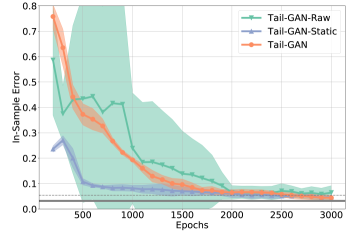
Figure 3: Training performance: relative error ${\rm RE}(1000)$ with 1000 samples. Grey horizontal line: average simulation error ${\rm SE}(1000)$. Dotted line: average simulation error plus one standard deviation. Each experiment is repeated five times with different random seeds. The performance is visualized with mean (solid lines) and standard deviation (shaded areas).

Performance accuracy.

We draw the following observations from Figure 3 and Table 1.

• For the evaluation criterion ${\rm RE}(1000)$ (see Figure 3), all three simulators, Tail-GAN-Raw, Tail-GAN-Static and Tail-GAN, converge within 2000 epochs with errors smaller than 10%. This implies that all three generators are able to capture the static information contained in the market data.

• For the evaluation criterion ${\rm RE}(1000)$, with both static portfolios and dynamic strategies on out-of-sample tests (see Table 1), only Tail-GAN converges to an error 4.6%, whereas the other two generators fail to capture the dynamic information in the market data.

• Compared to Tail-GAN-Raw and Tail-GAN-Static, Tail-GAN has the lowest training variance across multiple experiments (see standard deviations in Table 1). This implies that Tail-GAN has the most stable performance among all three simulators.

• Compared to Tail-GAN, WGAN yields a less competitive out-of-sample performance in terms of generating scenarios that have consistent tail risks of static portfolios and dynamic strategies. A possible explanation is that the objective function of WGAN focuses on the full distribution of raw returns, which does not guarantee the accuracy of tail risks of certain dynamic strategies.

	SE(1000)	HSM	Tail-GAN-Raw	Tail-GAN-Static	Tail-GAN	WGAN
OOS Error (%)	3.0	3.4	83.3	86.7	4.6	21.3
	(2.2)	(2.6)	(3.0)	(2.5)	(1.6)	(2.2)

Table 1: Mean and standard deviation (in parentheses) of relative errors for out-of-sample tests. Each experiment is repeated five times with different random seeds.

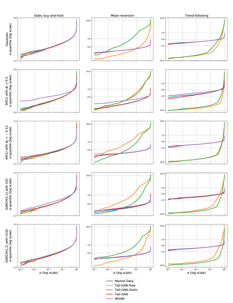
Figure 16: Tail behavior via the empirical rank-frequency distribution of the strategy PnL. The rows index the various models used for generating the ground truth synthetic data, while the columns index the strategy types.

Figure 4 shows the empirical quantile function of the strategy PnLs evaluated with price scenarios sampled from Tail-GAN-Raw, Tail-GAN-Static, Tail-GAN, and WGAN. The testing strategies are, from left to right (in Figure 4), static single-asset portfolio (buy-and-hold strategy), single-asset mean-reversion strategy and single-asset trend-following strategy. We only demonstrate here the performance of the AR(1) model, and the results for other assets are provided in Figure 16 in Appendix C. In each subfigure, we compare the rank-frequency distribution of strategy PnLs evaluated with input price scenario (in blue), three Tail-GAN simulators (in orange, red and green, resp.), and WGAN (in purple). Based on the results depicted in Figure 4, we conclude that

• All three variants of Tail-GAN are able to capture the tail properties of the static single-asset portfolio at quantile levels above 1%, as shown in the first column of Figure 4.

• For the PnL distribution of the dynamic strategies, only Tail-GAN is able to generate scenarios with compatible tail statistics of the PnL distribution, as shown in the second and third columns of Figure 4.

• Tail-GAN-Raw and Tail-GAN-Static underestimate the risk of the mean-reversion strategy at $\alpha=5\%$ quantile level, and overestimate the risk of the trend-following strategy at $\alpha=5\%$ quantile level, as illustrated in the second and third columns of Figure 4.

• It appears that WGAN fails to generate scenarios that retain consistent risk measures with the ground truth when the input market scenarios have heavy tails, such as AR(1) with autocorrelation 0.5, and GARCH(1,1) with $t(5)$ noise.

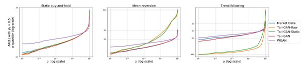
Figure 4: Tail behavior via the empirical rank-frequency distribution of the strategy PnL (based on AR(1) with autocorrelation $0.5$). The columns represent the strategy types.

Learning the temporal and correlation patterns.

Figures 5 and 6 show the correlation and auto-correlation patterns of market data (Figures 5(a) and 6(a)) and simulated data from Tail-GAN-Raw (Figures 5(b) and 6(b)), Tail-GAN-Static (Figures 5(c) and 6(c)), Tail-GAN (Figures 5(d) and 6(d)), and WGAN (Figures 5(e) and 6(e)).

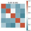
(a) Market data.

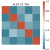
(b) Tail-GAN-Raw.

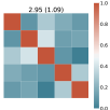
(c) Tail-GAN-Static.

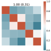
(d) Tail-GAN.

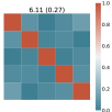
(e) WGAN.

Figure 5: Correlations of the price increments from different trained GAN models: (1) Tail-GAN-Raw, (2) Tail-GAN-Static, (3) Tail-GAN, and (4) WGAN. The numbers at the top of each plot denote the mean and standard deviation (in parentheses) of the sum of the absolute element-wise difference between the correlation matrices, computed with 10,000 training samples and 10,000 generated samples.

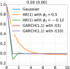
(a) Market Data.

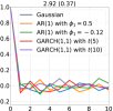
(b) Tail-GAN-Raw.

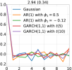
(c) Tail-GAN-Static.

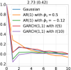
(d) Tail-GAN.

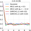
(e) WGAN.

Figure 6: Auto-correlations of the price increments from different trained GAN models: (1) Tail-GAN-Raw, (2) Tail-GAN-Static, (3) Tail-GAN, and (4) WGAN. The numbers at the top of each plot denote the mean and standard deviation (in parentheses) of the sum of the absolute difference between the auto-correlation coefficients computed with 10,000 training samples and 10,000 generated samples.

Figures 5 and 6 demonstrate that the auto-correlation and cross-correlations returns are best reproduced by Tail-GAN, trained on multi-asset dynamic portfolios. On the contrary, Tail-GAN-Raw and WGAN, trained on raw returns, have the lowest accuracy in this respect. This illustrates the importance of training the algorithm on benchmark strategies instead of only raw returns.

Statistical significance.

Table 2 summarizes the statistical test results for Historical Simulation Method, Tail-GAN-Raw, Tail-GAN-Static, Tail-GAN, and WGAN. Table 2 suggests that Tail-GAN achieves the lowest average rejection rate of the null hypothesis described in Section 4.2. In other words, scenarios generated by Tail-GAN have more consistent VaR and ES values for benchmark strategies compared to those of other simulators.

	HSM	Tail-GAN-Raw	Tail-GAN-Static	Tail-GAN	WGAN
Coverage Test (%)	17.9	53.6	22.9	17.1	44.9
Score-based Test (%)	0.00	21.3	15.4	0.00	11.4

Table 2: Average rejection rate of the null hypothesis in two tests across strategies. We use sample size $1,000$ and repeat the above experiment 100 times on testing data.

5.2 Discussion on the risk levels

In addition to the VaR and ES introduced in Section 2.1, the spectral risk measure (Kusuoka [2001]) is another well-known risk measure commonly used in the literature. For a distribution $\mu$, the spectral risk measure, denoted $\rho^{\phi}$, is defined as

$$\rho^{\phi}(\mu)=\int_{[0,1]}{\rm VaR}_{\alpha}(\mu)\,\phi({\rm d}\alpha),$$ (21)

where the spectrum $\phi$ is a probability measure on $[0,1]$. Theorem 5.2 in Fissler et al. [2016] shows that spectral risk measures under a spectral measure with finite support are jointly elicitable. We refer the reader to a class of score functions in Fissler et al. [2016]. This enables us to train Tail-GAN with multiple quantile levels $\{\alpha_{m}\}_{m=1}^{M}$ simultaneously. The theoretical developments in Section 3 could be generalized accordingly.

To further examine the robustness of our framework and verify that Tail-GAN is effective for not only one particular risk level, we evaluate the previously trained model Tail-GAN(5%) at some different levels. Here Tail-GAN$(a\%)$ represents Tail-GAN model trained at risk level $a$. As shown in the second column of Table 3, the performance of Tail-GAN(5%) is comparable to the baseline estimate SE(1000). We also train the model at a different level 10% (see Column Tail-GAN(10%)). We observe that Tail-GAN(10%) is slightly worse than Tail-GAN(5%) in terms of generating scenarios to match the tail risks at levels 1% and 5%, but better in 10%. Furthermore, we investigate the performance of Tail-GAN trained with multiple risk levels. In particular, the model Tail-GAN(1%&5%) is trained with the spectral risk measure defined in (21). The results suggest that, in general, including multiple levels can further improve the simulation accuracy.

OOS Error	SE(1000)	Tail-GAN(5%)	Tail-GAN(10%)	Tail-GAN(1%&5%)
$\alpha=1\%$	4.3	6.4	7.0	5.9
	(3.0)	(2.7)	(3.1)	(2.6)
$\alpha=5\%$	3.0	4.6	4.8	4.2
	(2.2)	(1.6)	(1.6)	(1.8)
$\alpha=10\%$	2.9	3.7	3.5	3.5
	(2.1)	(1.5)	(1.5)	(1.7)

Table 3: Mean and standard deviation (in parentheses) of relative errors for various risk levels. The columns represent the models trained for certain risks. The rows represent the out-of-sample performance for different risk levels.

5.3 Generalization error

If the training and test errors closely follow one another, it is said that a learning algorithm has good generalization performance, see Arora et al. [2017]. Generalization error quantifies the ability of machine learning models to capture certain inherent properties from the data or the ground-truth model. In general, machine learning models with a good generalization performance are meant to learn “underlying rules” associated with the data generation process, rather than only memorizing the training data, so that they are able to extrapolate learned rules from the training data to new unseen data. Thereby, the generalization error of a generator $G$ can be measured as the difference between the empirical divergence of the training data $d(\mathbb{P}_{r}^{(n)},\mathbb{P}_{G}^{(n)})$ and the ground-truth divergence $d(\mathbb{P}_{r},\mathbb{P}_{G})$.

To provide a systematic quantification of the generalization capability, we adopt the notion of generalization proposed in Arora et al. [2017]. For a fixed sample size $n$, the generalization error of $\mathbb{P}_{G}$ under divergence $d(\cdot,\cdot)$ is defined as

$$\left|d(\mathbb{P}_{r}^{(n)},\mathbb{P}_{G}^{(n)})-d(\mathbb{P}_{r},\mathbb{P}_{G})\right|,$$ (22)

where $\mathbb{P}_{r}^{(n)}$ is the empirical distribution of $\mathbb{P}_{r}$ with $n$ samples, i.e., the distribution of the training data, and $\mathbb{P}_{G}^{(n)}$ is the empirical distribution of $\mathbb{P}_{G}$ with $n$ samples drawn after the generator $G$ is trained. A small generalization error under definition (22) implies that GANs with good generalization property should have consistent performances with the empirical distributions (i.e., $\mathbb{P}_{r}^{(n)}$ and $\mathbb{P}_{G}^{(n)}$) and with the true distributions (i.e., $\mathbb{P}_{r}$ and $\mathbb{P}_{G}$). We consider two choices for the divergence function: $d_{q}$ based on quantile divergence, and $d_{s}$ based on the score function we use. See the mathematical definition in Appendix B.4.

To illustrate the generalization capabilities of Tail-GAN, we compare it with a supervised learning benchmark using the same loss function. Given the optimization problem (16)-(17), one natural idea is to construct a simulator (or a generator) using empirical VaR and ES values in the evaluation. To this end, we consider the following optimization

$$\min_{G\in\mathcal{G}}\frac{1}{Kn}\,\sum_{k=1}^{K}\sum_{j=1}^{n}S_{\alpha}\Big{(}\Big{(}{\mbox{VaR}_{\alpha}}\big{(}\Pi^{k}\#\mathbb{P}_{G}^{(n)}\big{)},{\mbox{ES}_{\alpha}}\big{(}\Pi^{k}\#\mathbb{P}_{G}^{(n)}\big{)}\Big{)},\,\,\Pi^{k}(\mathbf{p}_{j})\Big{)},$$ (23)

where $\mathbb{P}_{G}^{(n)}$ is the empirical measure of $n$ samples drawn from $\mathbb{P}_{G}$, and $\mathbf{p}_{j}$ are samples under the measure $\mathbb{P}_{r}$ ($j=1,2,\ldots,n$). The optimization problem (23) falls into the category of training simulators with supervised learning (Ostrovski et al. [2018]).

Compared with Tail-GAN, the presented supervised learning framework has several disadvantages, which we illustrate in a set of empirical studies. The first issue is the bottleneck in statistical accuracy. When using $\mathbb{P}_{r}^{(n)}$ as the guidance for supervised learning, as indicated in (23), it is not possible for the $\alpha$-VaR and $\alpha$-ES values of the simulated price scenarios $\mathbb{P}_{G}$ to improve on the sampling error of the empirical $\alpha$-VaR and $\alpha$-ES values estimated with the $n$ samples. In particular, ES is very sensitive to tail events, and the empirical estimate of ES may not be stable even with 10,000 samples. The second issue concerns the limited ability in generalization. A generator constructed via supervised learning tends to mimic the exact patterns in the input financial scenarios $\mathbb{P}_{r}^{(n)}$, instead of generating new scenarios that are equally realistic compared to the input financial scenarios under the evaluation of the score function.

We proceed to compare the performance of Tail-GAN with that of a Generator-Only Model (GOM) according to (23), from the point of view of both statistical accuracy and generalization ability. The detailed setup is provided in Appendix B.4.

Performance accuracy of Tail-GAN vs GOM.

Figure 7 reports the convergence of in-sample errors, and Table 4 summarizes the out-of-sample errors of GOM and Tail-GAN. From Table 4, we observe that the relative error of Tail-GAN is 4.6%, which is a 30% reduction compared to the relative error of GOM of around 7.2%. Compared to (23), the advantage of using neural networks to learn the VaR and ES values, as designed in Tail-GAN, is that it memorizes information in previous iterations during the training procedure, and therefore the statistical bottleneck with $n$ samples can be overcome when the number of iterations increases. Therefore, we conclude that Tail-GAN outperforms GOM in terms of simulation accuracy, demonstrating the importance of the discriminator.

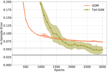
Figure 7: Training performance of GOM and Tail-GAN, as a function of the number of iterations in training. Grey horizontal line: average simulation error ${\rm SE}(1000)$. Dotted line: average simulation error plus one standard deviation. Each experiment is repeated five times with different random seeds. The performance is visualized with mean (solid lines) and standard deviation (shaded areas).

	Tail-GAN	GOM
OOS Error (%)	4.6	7.2
	(1.6)	(0.2)

Table 4: Mean and standard deviation (in parentheses) of relative errors for out-of-sample tests. Each experiment is repeated five times with different random seeds.

Table 5 provides the generalization errors, under both $d_{q}$ and $d_{s}$, for Tail-GAN and GOM. We observe that under both criteria, the generalization error of GOM is twice that of Tail-GAN, implying that Tail-GAN has better generalization power, in addition to higher performance accuracy.

Error metric	Tail-GAN	GOM
$d_{q}$	0.214	0.581
	(0.178)	(0.420)
$d_{s}$	0.017	0.032
	(0.014)	(0.026)

Table 5: Mean (in percentage) and standard deviation (in parentheses) of generalization errors under both divergence functions (see their mathematical formulations in (44) and (45)). Results are averaged over 10 repeated experiments (synthetic data sets).

5.4 Scalability

In practice, most portfolios held by asset managers are constructed with 20-30 or more financial assets. In order to scale Tail-GAN with a comparable number of assets, we use PCA-based eigenvectors. The resulting eigenportfolios (Avellaneda and Lee [2010]) are uncorrelated and able to explain the most variation in the cross-section of returns with the smallest number of portfolios. This idea enables to train Tail-GAN with the minimum number of portfolios, hence rendering Tail-GAN scalable to generate price scenarios with a large number of heterogeneous assets.

In this section, we train Tail-GAN with eigenportfolios of 20 assets, and compare its performance with Tail-GAN trained on 50 randomly generated portfolios. Tail-GAN with the eigenportfolios shows dominating performance, which is also comparable to simulation error (with the same number of samples). The detailed steps of the eigenportfolio construction are deferred to Appendix B.5.

Data.

To showcase the scalability of Tail-GAN, we simulate the price scenarios of 20 financial assets for a given correlation matrix $\mathbf{\rho}$, with different temporal patterns and tail behaviors in return distributions. Among these 20 financial assets, five of them follow Gaussian distributions, another five follow AR(1) models, another five of them follow GARCH(1, 1) with light-tailed noise, and the rest follow GARCH(1, 1) with heavy-tailed noise. Other settings are the same as in Section 5.1.

Results.

Figure 8 shows the percentage of explained variance of the principal components. We observe that the first principal component accounts for more than 23% of the total variation across the 20 asset returns.

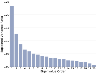
Figure 8: Explained variance ratios of eigenvalues.

To identify and demonstrate the advantages of the eigenportfolios, we compare the following two Tail-GAN architectures

1. Tail-GAN(Rand): GAN trained with 50 multi-asset portfolios and dynamic strategies,

2. Tail-GAN(Eig): GAN trained with 20 multi-asset eigenportfolios and dynamic strategies.

The weights of static portfolios in Tail-GAN(Rand) are randomly generated such that the absolute values of the weights sum up to one. The out-of-sample test consists of $K=90$ strategies, including 50 convex combinations of eigenportfolios (with weights randomly generated), 20 mean-reversion strategies, and 20 trend-following strategies.

Performance accuracy.

Figure 9 reports the convergence of in-sample errors. Table 6 summarizes the out-of-sample errors and shows that Tail-GAN(Eig) achieves better performance than Tail-GAN(Rand) with fewer number of portfolios.

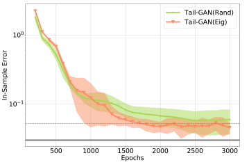
Figure 9: Training performance on 50 random portfolios vs 20 eigenportfolios as described in Section 5.4: mean of relative error RE(1000) and standard deviation (shaded areas). Grey horizontal line: average simulation error. Dotted line: average simulation error plus one standard deviation. Each experiment is repeated five times with different random seeds. The performance is reported with mean (solid lines) and standard deviation (shaded areas).

	HSM	Tail-GAN(Rand)	Tail-GAN(Eig)
OOS Error (%)	3.5	10.4	6.9
	(2.3)	(1.8)	(1.5)

Table 6: Mean and standard deviation (in parentheses) for relative errors in out-of-sample tests. Each experiment is repeated five times with different random seeds.

6 Application to simulation of intraday market scenarios

We use the Nasdaq ITCH data from LOBSTER during the intraday time interval 10:00AM-3:30PM, for the period 2019-11-01 until 2019-12-06. The reason for excluding the first and last 30 minutes of the trading day stems from the increased volatility and volume inherent in the market following the opening session, and preceding the closing session. The Tail-GAN simulator is trained on the following five stocks: AAPL, AMZN, GOOG, JPM, QQQ.

The mid-prices (average of the best bid and ask prices) of these assets are sampled at a $\Delta=9$-second frequency, with $T=100$ for each price series representing a financial scenario during a 15-minute interval. We sample the 15-minute paths every one minute, leading to an overlap of 14 minutes between two adjacent paths. The architecture and configurations are the same as those reported in Table 11 in Appendix B.2, except that the training period here is from 2019-11-01 to 2019-11-30, and the testing period is the first week of 2019-12. Thus, the size of the training data is $N=6300$. Table 7 reports the 5%-VaR and 5%-ES values of several strategies calculated with the market data of AAPL, AMZN, GOOG, JPM, and QQQ.

	Static buy-and-hold		Mean-reversion		Trend-following
	VaR	ES	VaR	ES	VaR	ES
AAPL	-0.351	-0.548	-0.295	-0.479	-0.316	-0.485
AMZN	-0.460	-0.720	-0.398	-0.639	-0.399	-0.628
GOOG	-0.316	-0.481	-0.272	-0.426	-0.273	-0.419
JPM	-0.331	-0.480	-0.275	-0.419	-0.290	-0.427
QQQ	-0.254	-0.384	-0.202	-0.321	-0.210	-0.328

Table 7: Empirical VaR and ES values for trading strategies evaluated on the training data.

Performance accuracy.

Figure 10 reports the convergence of in-sample errors and Table 8 summarizes the out-of-sample errors.

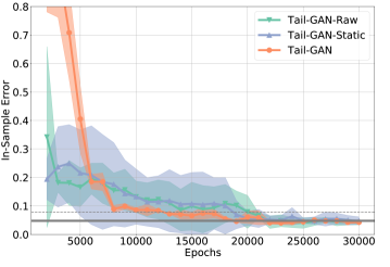
Figure 10: Training performance: relative error ${\rm RE}(1000)$ with 1000 samples. Grey horizontal line: average simulation error ${\rm SE}(1000)$. Dotted line: average simulation error plus one standard deviation. Each experiment is repeated 5 times with different random seeds. The performance is visualized with mean (solid lines) and standard deviation (shaded areas).

	“Oracle”	HSM	Tail-GAN-Raw	Tail-GAN-Static	Tail-GAN	WGAN
OOS Error (%)	2.4	10.4	112.8	75.8	10.1	26.9
	(1.6)	(3.6)	(7.8)	(8.0)	(1.1)	(1.7)

Table 8: Mean and standard deviation (in parentheses) for relative errors in out-of-sample tests. “Oracle” represents the sampling error of the testing data. Each experiment is repeated five times with different random seeds.

We draw the following conclusions from the results of Figure 10 and Table 8.

• For the evaluation criterion ${\rm RE}(1000)$ based on in-sample data (see Figure 10), all three GAN simulators, Tail-GAN-Raw, Tail-GAN-Static and Tail-GAN, converge within 20,000 epochs and reach in-sample errors smaller than 5%.

• For the evaluation criterion ${\rm RE}(1000)$, with both static portfolios and dynamic strategies based on out-of-sample data (Table 8), only Tail-GAN converges to an error of 10.1%, whereas the other two Tail-GAN variants fail to capture the temporal information in the input price scenarios.

• The HSM method comes close with an error of 10.4% and WGAN reaches an error of 26.9%. As expected, all methods attain higher errors than the sampling error of the testing data (denoted by “oracle” in Table 8).

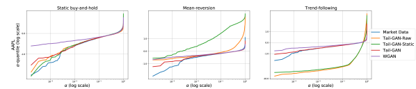
Figure 11: Tail behavior via the empirical rank-frequency distribution of the strategy PnL (based on AAPL). The columns represent the strategy types.

To study the tail behavior of the intraday scenarios, we implement the same rank-frequency analysis as in Section 5.1. For the AAPL stock, we draw the following conclusions from Figure 11

• All three Tail-GAN simulators are able to capture the tail properties of static single-asset portfolio for quantile levels above 1%.

• For the PnL distribution of the dynamic strategies, only Tail-GAN is able to generate scenarios with comparable (tail) PnL distribution. That is, only scenarios sampled from Tail-GAN can correctly describe the risks of the trend-following and the mean-reversion strategies.

• Tail-GAN-Raw and Tail-GAN-Static underestimate the risk of loss from the mean-reversion strategy at the $\alpha=5\%$ quantile level, and overestimate the risk of loss from the trend-following strategy at the $\alpha=5\%$ quantile level.

• While WGAN can effectively generate scenarios that align with the bulk of PnL distributions (e.g. above 10%-quantile), it tends to fail in accurately capturing the tail parts, usually resulting in underestimation of risks).

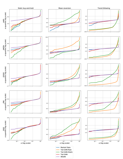
Figure 17: Tail behavior via the empirical rank-frequency distribution of the strategy PnL. The rows index various stocks, while the columns index the strategy types.

Note that some of the blue curves corresponding to the market data (almost) coincide with the red curves corresponding to Tail-GAN, indicating a promising performance of Tail-GAN to capture the tail risk of various trading strategies. See Figure 17 in Appendix C for the results for other assets.

Learning temporal and cross-correlation patterns.

Figures 12 and 13 present the in-sample correlation and auto-correlation patterns of the market data (Figures 12(a) and 13(a)), and simulated data from Tail-GAN-Raw (Figures 12(b) and 13(b)), Tail-GAN-Static (Figures 12(c) and 13(c)), Tail-GAN (Figures 12(d) and 13(d)) and WGAN (Figures 12(e) and 13(e)).

As shown in Figures 12 and 13, Tail-GAN trained on dynamic strategies learns the information on cross-asset correlations more accurately than Tail-GAN-Raw and WGAN, which are trained on raw returns.

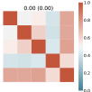
(a) Market data.

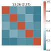
(b) Tail-GAN-Raw.

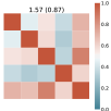
(c) Tail-GAN-Static.

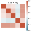
(d) Tail-GAN.

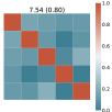
(e) WGAN.

Figure 12: Cross-asset correlations of the price increments in the market data and from different trained GAN models (1) Tail-GAN-Raw, (2) Tail-GAN-Static, (3) Tail-GAN, and (4) WGAN. Numbers on the top: mean and standard deviation (in parentheses) of the sum of the absolute difference between the correlation coefficients computed with all training samples and 1,000 generated samples.

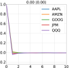
(a) Market data.

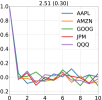
(b) Tail-GAN-Raw.

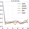
(c) Tail-GAN-Static.

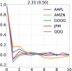
(d) Tail-GAN.

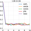
(e) WGAN.

Figure 13: Auto-correlations of the price increments from different trained GAN models: (1) Tail-GAN-Raw, (2) Tail-GAN-Static, (3) Tail-GAN, and (4) WGAN. Numbers on the top: mean and standard deviation (in parentheses) of the sum of the absolute element-wise difference between auto-correlation coefficients computed with all training samples and 1,000 generated samples.

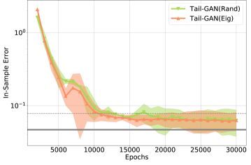
Figure 14: Training performance on 50 random portfolios vs 20 eigenportfolios, as in Section 5.4: mean of relative error ${\rm RE}(1000)$ and standard deviation (shaded areas). Grey horizontal line: average simulation error. Dotted line: average simulation error plus one standard deviation. Each experiment is repeated 5 times with different random seeds.

Scalability.

To test the scalability property of Tail-GAN on realistic scenarios, we conduct a similar experiment as in Section 5.4. The stocks considered here include the top 20 stocks in the S&P500 index. The training period is between 2019-11-01 and 2019-11-30.

Figure 14 reports the convergence of in-sample errors, and Table 9 summarizes the out-of-sample errors of Tail-GAN(Rand) and Tail-GAN(Eig). Table 9 shows that Tail-GAN(Eig) achieves better performance than Tail-GAN(Rand) with fewer training portfolios.

	“Oracle”	HSM	Tail-GAN(Rand)	Tail-GAN(Eig)
OOS Error (%)	2.2	25.9	31.0	25.6
	(1.7)	(5.1)	(1.0)	(1.0)

Table 9: Mean and standard deviation (in parentheses) for relative errors in out-of-sample tests. “Oracle” represents the sampling error of the testing data. Each experiment is repeated five times with different random seeds.

Appendix A Proofs

Proof of Proposition 2.2. First we check the elicitability condition for $H_{1}(v)$ and $H_{2}(e)$ on region $\mathcal{B}$. When $H_{2}(e)=\frac{\alpha}{2}e^{2}$, we have $H_{2}^{\prime}(e)=\alpha\,e$ and $H_{2}^{\prime\prime}(e)=\alpha$. For any $(v,e)\in\mathcal{B}$, this amounts to

$$\frac{\partial R_{\alpha}(v,e)}{\partial v}=e-W_{\alpha}v\geq 0,$$

where $R_{\alpha}(v,e)$ is defined in (1).

Recall the score function $S_{\alpha}(v,e,x)$ defined in (5), and $s_{\alpha}(v,e)$ defined in (4). Then

$$s_{\alpha}(v,e) = -(\mu(X\leq v)-\alpha)\frac{W_{\alpha}}{2}v^{2}+\frac{W_{\alpha}}{2}\int_{-\infty}^{v}x^{2}\mu(\mathrm{d}x)+\mu(X\leq v)v\,e$$

$$-e\int_{-\infty}^{v}x\mu(\mathrm{d}x)+\alpha e\left(\frac{e}{2}-v\right)+\text{const.}$$

Therefore,

$$\frac{\partial s_{\alpha}}{\partial v}(v,e) = \Big{(}\mu(X\leq v)-\alpha\Big{)}\left(-W_{\alpha}v+e\right),$$

$$\frac{\partial s_{\alpha}}{\partial e}(v,e) = \mu(X\leq v)v-\int_{-\infty}^{v}x\mu(\mathrm{d}x)+\alpha(e-v).$$

And hence

$$\frac{\partial^{2}s_{\alpha}}{\partial v^{2}}(v,e) = \frac{\mu(\mathrm{d}v)}{\mathrm{d}v}\left(-W_{\alpha}v+e\right)-W_{\alpha}(\mu(X\leq v)-\alpha),$$

$$\frac{\partial^{2}s_{\alpha}}{\partial e^{2}}(v,e) = \alpha,$$

$$\frac{\partial^{2}s_{\alpha}}{\partial e\partial v}(v,e) = \mu(X\leq v)-\alpha.$$

Since $\frac{\mu(X\in\mathrm{d}v)}{\mathrm{d}v}\geq 0$ and $-W_{\alpha}v+e>0$ hold on region $\mathcal{B}$, we have

$$\frac{\partial^{2}s_{\alpha}}{\partial v^{2}}(v,e)\geq-W_{\alpha}(\mu(X\leq v)-\alpha),\textit{ on }\mathcal{B}.$$

Therefore $\frac{\partial^{2}s_{\alpha}}{\partial v^{2}}(v,e)\geq 0$ holds since $v\leq{\rm VaR}_{\alpha}(\mu)$ on region $\mathcal{B}$. Next when $(v,e)\in\mathcal{B}$,

$$\frac{\partial^{2}s_{\alpha}}{\partial v^{2}}\frac{\partial^{2}s_{\alpha}}{\partial e^{2}}-\left(\frac{\partial^{2}s_{\alpha}}{\partial v\partial e}\right)^{2}=\alpha\,\frac{\mu(X\in\mathrm{d}v)}{\mathrm{d}v}\left(-W_{\alpha}v+e\right)-\alpha W_{\alpha}(\mu(X\leq v)-\alpha)-\left(\mu(X\leq v)-\alpha\right)^{2}$$ (24)

$$\geq (\alpha-\mu(X\leq v))(\alpha W_{\alpha}-\alpha+\mu(X\leq v))$$

$$\geq (\alpha-\mu(X\leq v))\mu(X\leq v)\geq 0.$$ (25)

Note that (24) holds since $-W_{\alpha}v+e\geq 0$, and (25) holds since $W_{\alpha}\geq 1$ and $\mu(X\leq v)\leq\alpha$ on $\mathcal{B}$. Therefore $\nabla^{2}\,s_{\alpha}$ is positive semi-definite on the region $\mathcal{B}$.

In addition, when condition (6) holds, we show that $s_{\alpha}(v,e)$ is positive semi-definite on $\widetilde{\mathcal{B}}$.

Denote $\widetilde{\mathcal{B}}^{1}=\widetilde{\mathcal{B}}\cap\big{\{}(v,e)\in\mathbb{R}^{2}\,|\,v\leq{\rm VaR}_{\alpha}(\mu)\big{\}}$ and $\widetilde{\mathcal{B}}^{2}=\widetilde{\mathcal{B}}\cap\{(v,e)\in\mathbb{R}^{2}|v>{\rm VaR}_{\alpha}(\mu)\}$. Then $\widetilde{\mathcal{B}}^{1}\cup\widetilde{\mathcal{B}}^{2}=\widetilde{\mathcal{B}}$ and $\widetilde{\mathcal{B}}^{1}\cap\widetilde{\mathcal{B}}^{2}=\emptyset$. The positive semi-definiteness property of $s_{\alpha}$ on $\widetilde{\mathcal{B}}^{1}$ follows a similar proof as above.

We only need to show that $s_{\alpha}$ is positive semi-definite on $\widetilde{\mathcal{B}}^{2}$. In this case, we have

$$\frac{\partial^{2}s_{\alpha}}{\partial v^{2}}(v,e) = \frac{\mu(\mathrm{d}v)}{\mathrm{d}v}\big{(}-W_{\alpha}v+e\big{)}-W_{\alpha}(\mu(X\leq v)-\alpha)$$ (26)

$$\geq \delta_{\alpha}\,z_{\alpha}-W_{\alpha}(\mu(X\leq v)-\alpha)\geq 0,$$

which holds since $\frac{\delta_{\alpha}\,z_{\alpha}}{W_{\alpha}}+\alpha\geq\beta_{\alpha}+\alpha\geq\mu(X\leq v)$ on $\widetilde{\mathcal{B}}$. In addition,

$$\frac{\partial^{2}s_{\alpha}}{\partial v^{2}}\frac{\partial^{2}s_{\alpha}}{\partial e^{2}}-\left(\frac{\partial^{2}s_{\alpha}}{\partial v\partial e}\right)^{2}=\alpha\,\frac{\mu(\mathrm{d}v)}{\mathrm{d}v}\left(-W_{\alpha}v+e\right)-\alpha W_{\alpha}(\mu(X\leq v)-\alpha)-\left(\mu(X\leq v)-\alpha\right)^{2}$$ (27)

$$\geq \alpha\delta_{\alpha}\,z_{\alpha}+(\mu(X\leq v)-\alpha)(-\alpha W_{\alpha}+\alpha-\mu(X\leq v))$$

$$\geq \alpha\delta_{\alpha}\,z_{\alpha}-\beta_{\alpha}(\alpha W_{\alpha}+\beta_{\alpha})\ \geq 0.$$ (28)

Here (27) holds since $\frac{\mu(\mathrm{d}v)}{\mathrm{d}v}\geq\delta_{\alpha}$ and $z_{\alpha}\geq\left(-W_{\alpha}v+e\right)$. (28) holds since $\mu(X\leq v)\in(\alpha,\alpha+\beta_{\alpha}]$ on $\widetilde{\mathcal{B}}^{2}$. To show (28), it suffices to show

$$\alpha\delta_{\alpha}\,z_{\alpha}-\frac{\delta_{\alpha}\,z_{\alpha}}{2W_{\alpha}}\left(\alpha W_{\alpha}+\frac{\delta_{\alpha}\,z_{\alpha}}{2W_{\alpha}}\right)\geq 0,$$ (29)

since $\beta_{\alpha}\leq\frac{\delta_{\alpha}\,z_{\alpha}}{2W_{\alpha}}$. Finally, (29) holds since $W_{\alpha}>\frac{1}{\sqrt{\alpha}}$, $\delta_{\alpha}\in(0,1)$, and $z_{\alpha}\in\left(0,\frac{1}{2}-\alpha\right)$. This completes the proof. $\blacksquare$

Proof of Theorem 3.3. Step 1. Consider the optimal transport problem in the semi-discrete setting: the source measure $\mathbb{P}_{z}$ is continuous and the target measure $P_{n}$ is discrete. Under Assumption 3.2, we can write $\mathbb{P}_{z}({\rm d}x)=m(x){\rm d}x$ for some probability density $m$. $P_{n}$ is discrete and we can write $P_{n}=\sum_{i=1}^{n}\nu_{i}\delta_{y_{i}}$ for some $\{y_{i}\}_{i=1}^{n}\subset\mathbb{R}^{M\times T}$, $\nu_{j}\geq 0$ and $\sum_{j=1}^{n}\nu_{j}=1$. In this semi-discrete setting, the Monge’s problem is defined as

$$\inf_{\Phi}\int\frac{1}{2}\|x-\Phi(x)\|^{2}m(x){\rm d}x\quad\text{ s.t. }\int_{\Phi^{-1}(y_{j})}{\rm d}\mathbb{P}_{z}=\nu_{j},\,\,j=1,2,\cdots,n.$$ (30)

In this case, the transport map assigns each point $x\in\mathbb{R}^{M\times T}$ to one of these $y_{j}$. Moreover, by taking advantage of the discreteness of the measure $\nu$, one sees that the dual Kantorovich problem in the semi-discrete case is maximizing the following functional:

$$\mathcal{F}(\psi)=\mathcal{F}(\psi_{1},\cdots,\psi_{n})=\int\inf_{j}\Big{(}\frac{1}{2}\|x-y_{j}\|^{2}-\psi_{j}\Big{)}m(x){\rm d}x+\sum_{j=1}^{n}\psi_{j}\nu_{j}.$$ (31)

The optimal transport map of the Monge’s problem (30) can be characterized by the maximizer of $\mathcal{F}$. To see this, let us introduce the concept of power diagram. Given a finite set of points $\{y_{j}\}_{j=1}^{n}\subset\mathbb{R}^{M\times T}$ and the scalars $\psi=\{\psi_{j}\}_{j=1}^{n}$, the power diagrams associated to the scalars $\psi$ and the points $\{y_{j}\}_{j=1}^{n}$ are the sets:

$$S_{j}=\left\{x\in\mathbb{R}^{M\times T}\,\,\,\,\left|\,\,\,\,\frac{1}{2}\|x-y_{j}\|^{2}-\psi_{j}\leq\frac{1}{2}\|x-y_{k}\|^{2}-\psi_{k},\,\forall k\neq j\right\}\right..$$

By grouping the points according to the power diagrams $S_{j}$, we have from (31) that

$$\mathcal{F}(\psi)=\sum_{j=1}^{n}\Big{[}\int_{S_{j}}\left(\frac{1}{2}\|x-y_{j}\|^{2}-\psi_{j}\right)m(x){\rm d}x+\psi_{j}\nu_{j}\Big{]}.$$ (32)

According to Theorem 4.2 in Lu and Lu [2020], the optimal transport plan $\Phi$ to solve the semi-discrete Monge’s problem is given by

$$\Phi(x)=\nabla\bar{\psi}(x),$$

where $\bar{\psi}(x)=\max_{j}\{x\cdot y_{j}+m_{j}\}$ for some $m_{j}\in\mathbb{R}$. Specifically, $\Phi(x)=y_{j}$ if $x\in S_{j}(x)$. Here $\psi=(\psi_{1},\cdots,\psi_{n})$ is an maximizer of $\mathcal{F}$ defined in (31) and $\{S_{j}\}_{j=1}^{n}$ denotes the power diagrams associated to $\{y_{j}\}_{j=1}^{n}$ and $\psi$.

Proposition 4.1 in Lu and Lu [2020] guarantees that there exists a feed-forward neural network $G(\cdot;\gamma)$ with $L=\lceil\log n\rceil$ fully connected layers of equal width $N=2^{L}$ and ReLU activation such that $\bar{\psi}(\cdot)=G(\cdot;\gamma)$.

Step 2. Denote $\mathbb{P}_{r}^{(n)}(\cdot):=\frac{1}{n}\sum_{i=1}^{n}{\bf 1}\{\cdot=\mathbf{p}_{i}\}$ as an empirical measure to approximate $\mathbb{P}_{r}\in\mathcal{P}(\mathbb{R}^{M\times T})$ using $n$ i.i.d. samples $\{\mathbf{p}_{i}\}_{i=1}^{n}$. Let $\{\Pi^{k}(\mathbf{p}_{[i]})\}_{i=1}^{n}$ be the order statistics of $\{\Pi^{k}(\mathbf{p}_{i})\}_{i=1}^{n}$, i.e., $\Pi^{k}(\mathbf{p}_{[1]})\leq\cdots\leq\Pi^{k}(\mathbf{p}_{[n]})$.

Let $\hat{v}_{n,\alpha}^{k}$ and $\hat{e}_{n,\alpha}^{k}$ denote the estimates of VaR and ES at level $\alpha$ using the $n$ samples above. These quantities are defined as follows (Serfling [2009]):

$$\hat{v}_{n,\alpha}^{k} = \Pi^{k}(\mathbf{p}_{[\lceil\alpha n\rceil]}),\text{ and }$$

$$\hat{e}_{n,\alpha}^{k} = \frac{1}{n(1-\alpha)}\sum_{i=1}^{n}\Pi^{k}(\mathbf{p}_{i}){\bf 1}\{\Pi^{k}(\mathbf{p}_{i})\leq\hat{v}_{n,\alpha}^{k}\}.$$

We first prove the result under the VaR criteria. According to Kolla et al. [2019, Proposition 2], with probability at least $\frac{1}{2}$ it holds that

$$\left|\hat{v}_{n,\alpha}^{k}-{\rm VaR}_{\alpha}(\Pi^{k}\#\mathbb{P}_{r})\right|\leq\sqrt{\frac{\log(4)}{2nc}},$$ (33)

where $c=c(\delta_{k},\eta_{k})$ is a constant that depends on $\delta_{k}$ and $\eta_{k}$, which are specified in Assumption A3. Setting the RHS of (33) as $\varepsilon$, we have $n=\mathcal{O}(\varepsilon^{-2})$. Under this choice of $n$, we have $\left|\hat{v}_{n,\alpha}^{k}-{\rm VaR}(\Pi^{k}\#\mathbb{P}_{r})\right|<\varepsilon$ holds with probability at least $\frac{1}{2}$. This implies that there must exist an empirical measure $\mathbb{P}_{r}^{(n)*}$ such that the corresponding $\hat{v}_{n,\alpha}^{k}$ satisfies $\left|\hat{v}_{n,\alpha}^{k}-{\rm VaR}(\Pi^{k}\#\mathbb{P}_{r})\right|<\varepsilon$. $\mathbb{P}_{r}^{(n)*}$ will be the target (empirical) measure we input in Step 1. This concludes the main result for the universal approximation under the VaR criteria.

We next prove the result under the ES criteria. Under Assumptions 3.1 and 3.2, we have

$$\mathbb{E}_{\mathbb{P}_{r}}\left[|\Pi^{k}(\mathbf{p})|^{\beta}\right]\leq(\ell_{k})^{\beta}\mathbb{E}_{\mathbb{P}_{r}}\left[\|\mathbf{p}\|^{\beta}\right]<\infty.$$ (34)

Take $n>\frac{16\log(8)}{(\eta_{k}\delta_{k}(1-\alpha))^{2}}$. Under (34) and Assumption A3, with probability $\frac{1}{2}$ it holds that

$$\left|\hat{e}_{n,\alpha}^{k}-{\rm ES}(\Pi^{k}\#\mathbb{P}_{r})\right| \leq \frac{\left(5\Big{(}\mathbb{E}_{\mathbb{P}_{r}}[\|\Pi^{k}(\mathbf{p})\|^{\beta}]\Big{)}^{1/\beta}-{\rm VaR}(\Pi^{k}\#\mathbb{P}_{r})\right)}{(1-\alpha)}\left(\frac{1}{n}\right)^{1-\frac{1}{\beta}}\sqrt{\log(6)}\noindent$$ (35)

$$\qquad+\frac{4}{\eta_{k}(1-\alpha)}\sqrt{\frac{\log(8)}{n}},$$

where $\eta_{k}$ and $\delta_{k}$ are as defined in A3. The result in (35) is a slight modification of Prashanth et al. [2020, Theorem 4.1]. Setting the RHS of (35) as $\varepsilon$, we have $n=\mathcal{O}(\varepsilon^{-\frac{\beta}{\beta-1}})$. Under this choice of $n$, we have $\left|\hat{e}_{n,\alpha}^{k}-{\rm ES}(\Pi^{k}\#\mathbb{P}_{r})\right|<\varepsilon$ holds with probability at least $\frac{1}{2}$. This implies that there must exist an empirical measure $\mathbb{P}_{r}^{(n)*}$ such that $\left|\hat{e}_{n,\alpha}^{k}-{\rm ES}(\Pi^{k}\#\mathbb{P}_{r})\right|<\varepsilon$ holds. $\mathbb{P}_{r}^{(n)*}$ will be the target (empirical) measure we input in Step 1. This concludes the main result for the universal approximation under the ES criterion. $\blacksquare$

Proof of Theorem 3.4. Step 1 is the same as Theorem 3.3. It is sufficient to prove the corresponding Step 2.

Step 2. Denote $\mathbb{P}_{r}^{(n)}(\cdot):=\frac{1}{n}\sum_{i=1}^{n}{\bf 1}\{\cdot=\mathbf{p}_{i}\}$ as an empirical measure to approximate $\mathbb{P}_{r}\in\mathcal{P}(\mathbb{R}^{M\times T})$ using $n$ i.i.d. samples $\{\mathbf{p}_{i}\}_{i=1}^{n}$. Denote $M_{\beta}:=\mathbb{E}_{\mathbb{P}_{r}}[\|\mathbf{p}\|^{\beta}]<\infty$. From Lei [2020, Theorem 3.1] we have

$$\mathbb{E}\mathcal{W}_{1}(\mu_{n},\mu)\leq c_{\beta}M_{\beta}n^{-\frac{1}{(2\beta)\vee(M\times T)}\wedge(1-\frac{1}{\beta})}(\log n)^{\zeta_{\beta,M\times T}},$$ (36)

where $c_{\beta}$ is a constant depending only on $\beta$ (not $M\times T$)

$$\zeta_{\beta,M\times T}=\begin{cases}2&\quad\textit{ if }M\times T=\beta=2,\\ 1&\quad\textit{ if }``M\times T\neq 2\textit{ and }\beta=\frac{M\times T}{M\times T-1}\wedge 2"\textit{ or }``\beta>M\times T=2",\\ 0&\quad\textit{ otherwise}.\end{cases}$$

By the Kantorovich-Rubenstein duality, we have

$$\mathcal{W}_{1}\Big{(}\Pi^{k}\#\mathbb{P}_{r},\Pi^{k}\#\mathbb{P}_{r}^{(n)}\Big{)} = {\frac{1}{\ell}}\sup_{\|f\|_{L}\leq\ell}\mathbb{E}_{\mathbf{p}\sim\mathbb{P}_{r}}\Big{[}f(\Pi^{k}(\mathbf{p}))\Big{]}-\mathbb{E}_{\mathbf{q}\sim\mathbb{P}_{r}^{(n)}}\Big{[}f(\Pi^{k}(\mathbf{q}))\Big{]}\noindent$$ (37)

$$\leq {\frac{1}{\ell}}\sup_{\|g\|_{L}\leq\ell\ell_{k}}\mathbb{E}_{\mathbf{p}\sim\mathbb{P}_{r}}\Big{[}g(\mathbf{p})\Big{]}-\mathbb{E}_{\mathbf{q}\sim\mathbb{P}_{r}^{(n)}}\Big{[}g(\mathbf{q})\Big{]}$$ (38)

$$\leq \ell_{k}\mathcal{W}_{1}\Big{(}\mathbb{P}_{r},\mathbb{P}_{r}^{(n)}\Big{)}$$ (39)

where $\|\cdot\|_{L}$ is the Lipschitz norm. (38) holds since $f(\Pi^{k}(\cdot))$ is $\ell\ell_{k}$-Lipschitz when $f$ is $\ell$-Lipschitz and $\Pi^{k}$ is $\ell_{k}$-Lipschitz. (39) holds by the Kantorovich-Rubenstein duality.

Taking expectation on (15) and applying (36) and (39), we have

$$\mathbb{E}\Big{|}\rho(\Pi^{k}\#\mathbb{P}_{r})-\rho(\Pi^{k}\#\mathbb{P}_{r}^{(n)})\Big{|} \leq L\mathbb{E}\Big{(}\mathcal{W}_{1}\Big{(}\Pi^{k}\#\mathbb{P}_{r},\,\Pi^{k}\#\mathbb{P}_{r}^{(n)}\Big{)}\Big{)}^{\kappa}$$ (40)

$$\leq L\Big{(}\mathbb{E}\left[\mathcal{W}_{1}\Big{(}\Pi^{k}\#\mathbb{P}_{r},\,\Pi^{k}\#\mathbb{P}_{r}^{(n)}\Big{)}\right]\Big{)}^{\kappa}$$ (41)

$$\leq L\Big{(}\ell_{k}c_{\beta}M_{\beta}n^{-\frac{1}{2\vee d}\wedge(1-\frac{1}{\beta})}(\log n)^{\zeta_{\beta,M\times T}}\Big{)}^{\kappa},$$ (42)

where (41) holds by Jensen’s inequality since $\kappa\in(0,1]$.

(40) implies that there must exist an empirical measure $\mathbb{P}_{r}^{(n)*}$ such that $\Big{|}\rho(\Pi^{k}\#\mathbb{P}_{r})-\rho(\Pi^{k}\#\mathbb{P}_{r}^{(n)})\Big{|}<\varepsilon$ holds. This $\mathbb{P}_{r}^{(n)*}$ will be the target (empirical) measure we input in Step 1.

It is easy to check that

• $\frac{1}{2\vee(M\times T)}\wedge(1-\frac{1}{\beta})=1-\frac{1}{\beta}$ when $M=T=1$ and $1<\beta\leq 2$;

• $\frac{1}{2\vee(M\times T)}\wedge(1-\frac{1}{\beta})=\frac{1}{2}$ when $M=T=1$ and $\beta\geq 2$;

• $\frac{1}{2\vee(M\times T)}\wedge(1-\frac{1}{\beta})=\frac{1}{M\times T}$ when $M\times T\geq 2$ and $\frac{1}{M\times T}+\frac{1}{\beta}<1$;

• $\frac{1}{2\vee(M\times T)}\wedge(1-\frac{1}{\beta})=1-\frac{1}{\beta}$ when $M\times T\geq 2$ and $\frac{1}{M\times T}+\frac{1}{\beta}\geq 1$.

This concludes the main result for the universal approximation under risk measures that are Hölder continuous. $\blacksquare$

Proof of Theorem 3.6..

For any $\overline{D}\in\overline{\mathcal{D}}_{0}$, by definition there exists $\mu:=\mu(\overline{D})\in\mathcal{P}(\mathbb{R}^{M\times T})$ with a finite first moment such that

$$\overline{D}(\Pi^{k}\#\mu)=\Big{(}{\rm VaR}_{\alpha}(\Pi^{k}\#\mathbb{P}_{r}),{\rm ES}_{\alpha}(\Pi^{k}\#\mathbb{P}_{r})\Big{)},\quad\forall k=1,2,\cdots,K.$$ (43)

Denote $\Sigma(\overline{D})$ as the set of all such $\mu\in\mathcal{P}(\mathbb{R}^{M\times T})$ with finite first moment that satisfies (43). Then given that both $\mu\in\Sigma(\overline{D})$ and $\mathbb{P}_{z}$ have finite first moments and that $\mathbb{P}_{z}$ is absolutely continuous with respect to the Lebesgue measure, we could find a mapping $\overline{G}\in\overline{\mathcal{G}}$ such that $\overline{G}\#\mathbb{P}_{{z}}\in\Sigma(\overline{D})$ so that $\mathbb{E}_{\mathbf{p}\sim\mathbb{P}_{r}}\left[\,\,S_{\alpha}\Big{(}\overline{D}\big{(}\Pi^{k}\#\mathbb{P}_{\overline{G}}\big{)},\Pi^{k}(\mathbf{p})\Big{)}\right]$ is minimized (Theorem 7.1 in Ambrosio et al. [2003]). That is,

$$\min_{\overline{G}\in\overline{\mathcal{G}}}\frac{1}{K}\sum_{k=1}^{K}\mathbb{E}_{\mathbf{p}\sim\mathbb{P}_{r}}\left[\,\,S_{\alpha}\Big{(}\overline{D}\big{(}\Pi^{k}\#\mathbb{P}_{\overline{G}}\big{)},\Pi^{k}(\mathbf{p})\Big{)}\right]=\frac{1}{K}\sum_{k=1}^{K}\mathbb{E}_{\mathbf{p}\sim\mathbb{P}_{r}}\left[\,\,S_{\alpha}\Big{(}\Big{(}{\rm VaR}_{\alpha}(\Pi^{k}\#\mathbb{P}_{r}),{\rm ES}_{\alpha}(\Pi^{k}\#\mathbb{P}_{r})\Big{)},\Pi^{k}(\mathbf{p})\Big{)}\right].$$

In this case, for the maximization problem of $\overline{D}$ over $\overline{\mathcal{D}}_{0}$,

$$\eqref{newminimax_distribution} = \max_{\overline{D}\in\overline{\mathcal{D}}_{0}}\ \frac{1}{K}\,\sum_{k=1}^{K}\Bigg{[}\mathbb{E}_{\mathbf{p}\sim\mathbb{P}_{r}}\left[\,\,S_{\alpha}\Big{(}\Big{(}{\rm VaR}_{\alpha}(\Pi^{k}\#\mathbb{P}_{r}),{\rm ES}_{\alpha}(\Pi^{k}\#\mathbb{P}_{r})\Big{)},\Pi^{k}(\mathbf{p})\Big{)}\right]-\lambda\,\,\mathbb{E}_{\mathbf{p}\sim\mathbb{P}_{r}}\left[S_{\alpha}\Big{(}\overline{D}(\Pi^{k}\#\mathbb{P}_{r}),\,\,\Pi^{k}(\mathbf{p})\Big{)}\right]\,\,\Bigg{]}$$

$$= -\lambda\min_{\overline{D}\in\overline{\mathcal{D}}_{0}}\frac{1}{K}\,\sum_{k=1}^{K}\mathbb{E}_{\mathbf{p}\sim\mathbb{P}_{r}}\left[S_{\alpha}\Big{(}\overline{D}(\Pi^{k}\#\mathbb{P}_{r}),\,\,\Pi^{k}(\mathbf{p})\Big{)}\right].$$

By the definition of $\overline{\mathcal{D}}_{0}$, we have

$$\min_{\overline{D}\in\overline{\mathcal{D}}_{0}}\frac{1}{K}\,\sum_{k=1}^{K}\mathbb{E}_{\mathbf{p}\sim\mathbb{P}_{r}}\left[S_{\alpha}\Big{(}\overline{D}(\Pi^{k}\#\mathbb{P}_{r}),\,\,\Pi^{k}(\mathbf{p})\Big{)}\right]$$

$$= \frac{1}{K}\,\sum_{k=1}^{K}\mathbb{E}_{\mathbf{p}\sim\mathbb{P}_{r}}\left[S_{\alpha}\Big{(}\Big{(}{\rm VaR}_{\alpha}(\Pi^{k}\#\mathbb{P}_{r}),{\rm ES}_{\alpha}(\Pi^{k}\#\mathbb{P}_{r})\Big{)},\,\,\Pi^{k}(\mathbf{p})\Big{)}\right]$$

$$= \min_{\overline{D}\in\overline{\mathcal{D}}}\frac{1}{K}\,\sum_{k=1}^{K}\mathbb{E}_{\mathbf{p}\sim\mathbb{P}_{r}}\left[S_{\alpha}\Big{(}\overline{D}(\Pi^{k}\#\mathbb{P}_{r}),\,\,\Pi^{k}(\mathbf{p})\Big{)}\right],$$

which is equivalent to (17). Denote this minimizer as $\overline{D}^{*}$, plugging this into the optimization problem for $\overline{G}$ in the max-min game leads to the upper-level optimization problem (16). ∎

Appendix B Implementation details

B.1 Setup of parameters in the synthetic data set

Mathematically, for any given time $t\in[0,T]$, we first sample $\mathbf{u}_{t}=(u_{1,t},\ldots,u_{5,t})^{\top}\sim\mathcal{N}(0,\Sigma)$ with covariance matrix $\Sigma\in\mathbb{R}^{5\times 5}$, $v_{1,t}\sim\chi^{2}(\nu_{1})$ and $v_{2,t}\sim\chi^{2}(\nu_{2})$. Here $v_{1,t}$, $v_{2,t}$ are independent of $\mathbf{u}_{t}$. We then calculate the price increments according to the following equations

$$\Delta p_{1,t} =u_{1,t},$$

$$\Delta p_{2,t} =\phi_{1}\Delta p_{2,t-1}+u_{2,t},$$

$$\Delta p_{3,t} =\phi_{2}\Delta p_{3,t-1}+u_{3,t},$$

$$\Delta p_{4,t} =\varepsilon_{4,t}=\sigma_{4,t}\eta_{1,t},$$

$$\Delta p_{5,t} =\varepsilon_{5,t}=\sigma_{5,t}\eta_{2,t},$$

where $\sigma_{4,t}^{2}=\gamma_{4}+\kappa_{4}\varepsilon_{4,t-1}^{2}+\beta_{4}\sigma_{4,t-1}^{2},\eta_{1,t}=\frac{u_{4,t}}{\sqrt{v_{1,t}/\nu_{1}}},$ and $\sigma_{5,t}^{2}=\gamma_{5}+\kappa_{5}\varepsilon_{5,t-1}^{2}+\beta_{5}\sigma_{5,t-1}^{2},\eta_{2,t}=\frac{u_{5,t}}{\sqrt{v_{2,t}/\nu_{2}}}$.

We set $T=100$ as the number of observations over one trading day. We first generate a correlation matrix $\rho$ with elements uniformly sampled from $[0,1]$. We then sample the annualized standard deviations $s$ with values between $0.3$ and $0.5$, and set $\Sigma_{ij}=\frac{s_{i}}{255\times T}\frac{s_{j}}{255\times T}\rho_{ij}$ ($i,j=1,2,\ldots,5$); $\phi_{1}=0.5$ and $\phi_{2}=-0.15$; $\nu_{1}=5$ and $\nu_{2}=10$; $\kappa_{4}$ and $\kappa_{5}$ are sampled uniformly from [0.08, 0.12]; $\beta_{4}$ and $\beta_{5}$ are sampled uniformly from [0.825, 0.875]; and finally $\gamma_{4}$ and $\gamma_{5}$ are sampled uniformly from [0.03, 0.07]. We choose one quantile $\alpha=0.05$ for this experiment.

Table 10 reports the 5%-VaR and 5%-ES values of several strategies calculated with the synthetic financial scenarios designed above.

	Static buy-and-hold		Mean-reversion		Trend-following
	VaR	ES	VaR	ES	VaR	ES
Gaussian	-0.489	-0.615	-0.432	-0.553	-0.409	-0.515
AR(1) with $\phi_{1}=0.5$	-0.876	-1.100	-0.850	-1.066	-0.671	-0.829
AR(1) with $\phi_{2}=-0.12$	-0.461	-0.581	-0.399	-0.513	-0.387	-0.488
GARCH(1,1) with $t(5)$	-0.480	-0.603	-0.420	-0.535	-0.400	-0.501
GARCH(1,1) with $t(10)$	-0.403	-0.507	-0.354	-0.453	-0.328	-0.410

Table 10: Empirical VaR and ES values for trading strategies evaluated on the training data.

B.2 Setup of the configuration

	Configuration	Values
Discriminator	Architecture	Fully-connected layers
	Activation	Leaky ReLU
	Number of neurons in each layer	(1000, 256, 128, 2)
	Learning rate	$10^{-7}$
	Dual parameter ($\lambda$)	$1$
	Batch normalization	No
Generator	Architecture	Fully-connected layers
	Activation	Leaky ReLU
	Number of neurons in each layer	(1000, 128, 256, 512, 1024, $5\times 100$)
	Learning rate	$10^{-6}$
	Batch normalization	Yes
Strategies	Static portfolio with single asset	5
	Static portfolio with multiple assets	50
	Mean-reversion strategies	5
	Trend-following strategies	5
Additional parameters	Size of training data ($N$)	50,000
	Number of PnL samples ($N_{B}$)	1,000
	Noise dimension ($N_{z}$)	1,000
	Noise distribution	$t(5)$
	$H_{1},{H}_{2}$	$H_{1}(v)=-5v^{2}$, ${H}_{2}(e)=\frac{\alpha}{2}e^{2}$

Table 11: Network architecture configuration.

Discussion on the configuration.

• Choice of $\lambda$: Theorem 3.6 suggests that Tail-GAN is effective as long as $\lambda>0$. In our experiments, we set $\lambda=1$ and also tested values of 2, 10, and 100 to address the issue of hyper-parameter selection. We observed that $\lambda=2$ and $\lambda=10$ resulted in a similar performance to $\lambda=1$, while larger values such as $\lambda=100$ led to a worse performance similar to that of the supervised learning method. This may be due to the fact that larger $\lambda$ values could potentially harm the model’s generalization power in practical settings.

• Choice of $S_{\alpha}$ ($H_{1}$ and $H_{2}$): Proposition 2.2 demonstrates that choosing $H_{1}$ and $H_{2}$ as quadratic functions (as proposed in Acerbi and Szekely [2014]) results in a positive semi-definite score function in a neighborhood region around the global minimum. This is the first theoretical evidence that highlights the optimization landscape advantages of selecting quadratic functions for $H_{1}$ and $H_{2}$.

• Neural network architecture: Theorem 3.3 implies that a feed-forward neural network with fully connected layers of equal width and ReLU activation is capable of generating financial scenarios that are arbitrarily close to the scenarios sampled from the true distribution $\mathbb{P}_{r}$ under VaR and ES criteria. This sheds light on using a simple network architecture such as multi-layer perceptron (MLP) in the training of Tail-GAN.

  While a more sophisticated neural network architecture may improve practical performance, our focus is not to compare different architectures, but rather to demonstrate the benefits of incorporating the essential component of tail risks of trading strategies into our Tail-GAN framework. Therefore, we choose to use a simple MLP, the same architecture used in Wasserstein GAN (Arjovsky et al. [2017]). On the other hand, it has been reported in recent literature that simple and shallow neural network architectures attain better performance on financial applications compared to more advanced architectures (Gu et al. [2020], Chen et al. [2023]).

B.3 Differentiable neural sorting

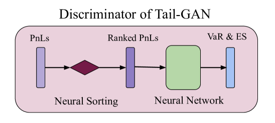
Figure 15: Architecture of the Tail-GAN discriminator.

The architecture of the Tail-GAN Discriminator has two key ingredients, as depicted in Figure 15. For the first ingredient, a differentiable sorting algorithm proposed by Grover et al. [2019] is employed to rank the PnLs. The second part adopts a standard neural network architecture, taking the ranked PnLs as the input, and providing the estimated $\alpha$-VaR and $\alpha$-ES values as the output.

We follow the design in Grover et al. [2019] to include the differentiable sorting architecture, so that the input of the discriminator will be the ranked PnL’s (sorted in decreasing order). This design, based on the idea of using the soft-max operator to approximate the arg-max operator, enables back-propagation of the gradient of the sorting function during the network training process.

Denote $\mathbf{x}^{k}=(x^{k}_{1},x^{k}_{2},\ldots,x^{k}_{n})^{\top}$ as a real-valued vector of length $n$, representing the PnL samples of strategy $k$. Let $B({\mathbf{x}^{k}})$ denote the matrix of absolute pairwise differences of the elements of $\mathbf{x}^{k}$, such that $B_{i,j}(\mathbf{x}^{k})=|x_{i}^{k}-x_{j}^{k}|$. We then define the following permutation matrix $\Gamma(\mathbf{x}^{k})$ following Grover et al. [2019], Ogryczak and Tamir [2003]

$$\Gamma_{i,j}(\mathbf{x}^{k})=\begin{cases}1,\quad\mbox{ if }j=\arg\max((n+1-2i)-B(\mathbf{x}^{k}){\bf 1}),\\ 0,\quad\mbox{otherwise},\end{cases}$$

where $\bf 1$ is the all-ones vector. Then, $\Gamma(\mathbf{x}^{k})\mathbf{x}^{k}$ provides a ranked vector of $\mathbf{x}^{k}$ (Ogryczak and Tamir [2003, Lemma 1] and Grover et al. [2019, Corollary 3]). However, the arg-max operator is non-differentiable which prohibits the direct usage of the permutation matrix for gradient computation. Instead, Grover et al. [2019] propose to replace the arg-max operator with soft-max, in order to obtain a continuous relaxation $\widehat{\Gamma}^{\tau}$ with a temperature parameter $\tau>0$. In particular, the $(i,j)$-th element of $\widehat{\Gamma}^{\tau}(\mathbf{x}^{k})$ is given by

$$\widehat{\Gamma}^{\tau}_{i,j}(\mathbf{x}^{k})=\frac{\exp\big{(}\big{(}(n+1-2i)-B(\mathbf{x}^{k})_{j}{\bf 1}\big{)}/\tau\big{)}}{\sum_{l=1}^{n}\exp\big{(}\big{(}(n+1-2i)-B(\mathbf{x}^{k})_{l}{\bf 1}\big{)}/\tau\big{)}},$$

in which $B(\mathbf{x}^{k})_{l}$ is the $l$-th row of matrix $B(\mathbf{x}^{k})$. This relaxation is continuous everywhere and differentiable almost everywhere with respect to the elements of $\mathbf{x}^{k}$. In addition, Grover et al. [2019, Theorem 4] shows that $\widehat{\Gamma}^{\tau}_{i,j}(\mathbf{x}^{k})$ converges to $\Gamma_{i,j}(\mathbf{x}^{k})$ almost surely when $x^{k}_{1},\ldots,x^{k}_{n}$ are sampled IID from a distribution which is absolutely continuous with respect to the Lebesgue measure in $\mathbb{R}$.

Finally we could set in (11):

$$\widetilde{\Gamma}(\mathbf{x})=\widehat{\Gamma}^{\tau}(\mathbf{x})\mathbf{x}.$$

B.4 Divergence functions and GOM

Divergence functions.

Here, we provide two choices for the divergence function. First, the quantile divergence between two distributions $P$ and $Q$ is defined as Ostrovski et al. [2018]

$$q(P,Q):=\int_{0}^{1}\left[\int_{F_{P}^{-1}(\tau)}^{F_{Q}^{-1}(\tau)}\left(F_{P}(x)-\tau\right)\mathrm{d}x\right]\mathrm{d}\tau,$$

where $F_{P}$ (resp. $F_{Q}$) is the CDF of $P$ (resp. $Q$). Motivated by this definition of quantile divergence, we propose the following local-“divergence”, which focuses on the tail distribution of the strategy PnLs

$$d_{q}(\mathbb{P}_{r},\mathbb{P}_{G}):=\frac{1}{K}\sum_{k=1}^{K}\int_{0}^{\alpha}\left[\int_{F_{\Pi^{k}\#\mathbb{P}_{r}}^{-1}(\tau)}^{F_{\Pi^{k}\#\mathbb{P}_{G}}^{-1}(\tau)}\left(F_{\Pi^{k}\#\mathbb{P}_{r}}(x)-\tau\right)\mathrm{d}x\right]\mathrm{d}\tau,$$ (44)

where $F_{\Pi^{k}\#\mathbb{P}_{r}}$ (resp. $F_{\Pi^{k}\#\mathbb{P}_{G}}$) is the CDF of $\Pi^{k}(\mathbf{p})$ with $\mathbf{p}\sim\mathbb{P}_{r}$ (resp. $\Pi^{k}(\mathbf{q})$ with $\mathbf{q}\sim\mathbb{P}_{G}$). Recall that the score function used in the loss function (18) can also be constructed as a “divergence” to measure the difference between two distributions in terms of their respective VaR and ES values

$$d_{s}\left({\mathbb{P}}_{r},{\mathbb{P}}_{G}\right):=\frac{1}{K}\sum_{k=1}^{K}\mathbb{E}_{\mathbf{p}\sim\mathbb{P}_{r}} \Bigg{[}S_{\alpha}\big{(}{\rm VaR}_{\alpha}\left(\Pi^{k}\#\mathbb{P}_{G}\right),{\rm ES}_{\alpha}\left(\Pi^{k}\#\mathbb{P}_{G}\right),{\Pi^{k}(\mathbf{p})}\big{)}$$ (45)

$$-S_{\alpha}\big{(}{\rm VaR}_{\alpha}\left(\Pi^{k}\#\mathbb{P}_{r}\right),{\rm ES}_{\alpha}\left(\Pi^{k}\#\mathbb{P}_{r}\right),{\Pi^{k}(\mathbf{p})}\big{)}\Bigg{]}.$$

Setup for GOM.

We follow the procedure in Section B.3 and use $\left(x^{k}_{(\lfloor\alpha n\rfloor{})},\frac{1}{\lfloor\alpha n\rfloor{}}\sum_{i=1}^{\lfloor\alpha n\rfloor{}}x^{k}_{(i)}\right)$ to estimate the $\alpha$-VaR and $\alpha$-ES values, where $x^{k}_{(n)}\geq\ldots\geq x^{k}_{(2)}\geq x^{k}_{(1)}$ are the sorted PnLs of $\mathbf{x}^{k}$ via the differentiable neural sorting architecture. We train the GOM on synthetic price scenarios, with both multi-asset portfolio and dynamic strategies. The setting of GOM is the same as that of Tail-GAN (described in Table 11), except that there is no discriminator.

B.5 Construction of eigenportfolios

We construct eigenportfolios from the principal components of the empirical correlation matrix $\hat{\mathbf{\rho}}$ of returns, ranked in decreasing order of eigenvalues: $\hat{\mathbf{\rho}}=\mathbf{Q}\mathbf{\Lambda}\mathbf{Q}^{-1}$ where $\mathbf{Q}$ is the orthogonal matrix with the $i$-th column being the eigenvector $\mathbf{q}_{i}\in\mathbb{R}^{M}$ of $\hat{\mathbf{\rho}}$, and $\mathbf{\Lambda}$ is the diagonal matrix whose diagonal elements are the corresponding eigenvalues, such that $\mathbf{\Lambda}_{1,1}\geq\mathbf{\Lambda}_{2,2}\geq\dots\geq\mathbf{\Lambda}_{M,M}\geq 0$.

Eigenportfolios are constructed from the principal components as follows. Denote $\mathbf{h}={\rm diag}{(\sigma_{1},\dots,\sigma_{M})}$, where $\sigma_{i}$ is the empirical standard deviation of asset $i$. For the $i$-th eigenvector $\mathbf{q}_{i}$, we consider its corresponding eigenportfolio

$$\frac{{(\mathbf{h}^{-1}\mathbf{q}_{i})}^{T}\mathbf{p}}{\|\mathbf{h}^{-1}\mathbf{q}_{i}\|_{1}},$$

where $\mathbf{p}\in\mathbb{R}^{M\times T}$ is the price scenario, and $\|\mathbf{h}^{-1}\mathbf{q}_{i}\|_{1}$ is used to normalize the portfolio weights so that the absolute weights sum to unity.

Appendix C Additional numerical experiments

References

- Acerbi [2002] Carlo Acerbi. Spectral measures of risk: A coherent representation of subjective risk aversion. Journal of Banking & Finance, 26(7):1505–1518, 2002.
- Acerbi and Szekely [2014] Carlo Acerbi and Balazs Szekely. Back-testing expected shortfall. Risk, 27(11):76–81, 2014.
- Ambrosio et al. [2003] Luigi Ambrosio, Luis A Caffarelli, Yann Brenier, Giuseppe Buttazzo, Cedric Villani, Sandro Salsa, Luigi Ambrosio, and Aldo Pratelli. Existence and stability results in the l 1 theory of optimal transportation. Optimal Transportation and Applications: Lectures given at the CIME Summer School, held in Martina Franca, Italy, September 2-8, 2001, pages 123–160, 2003.
- Arjovsky et al. [2017] Martin Arjovsky, Soumith Chintala, and Léon Bottou. Wasserstein generative adversarial networks. In International conference on machine learning, pages 214–223. PMLR, 2017.
- Arora et al. [2017] Sanjeev Arora, Rong Ge, Yingyu Liang, Tengyu Ma, and Yi Zhang. Generalization and equilibrium in generative adversarial nets (gans). In International Conference on Machine Learning, pages 224–232. PMLR, 2017.
- Avellaneda and Lee [2010] Marco Avellaneda and Jeong-Hyun Lee. Statistical arbitrage in the US equities market. Quantitative Finance, 10(7):761–782, 2010.
- Bank for International Settlements [2019] Bank for International Settlements. Minimum capital requirements for market risk. https://www.bis.org/bcbs/publ/d457.pdf, 2019.
- Ben-Tal and Teboulle [1986] Aharon Ben-Tal and Marc Teboulle. Expected utility, penalty functions, and duality in stochastic nonlinear programming. Management Science, 32(11):1445–1466, 1986.
- Ben-Tal and Teboulle [2007] Aharon Ben-Tal and Marc Teboulle. An old-new concept of convex risk measures: the optimized certainty equivalent. Mathematical Finance, 17(3):449–476, 2007.
- Bhatia et al. [2020] Siddharth Bhatia, Arjit Jain, and Bryan Hooi. ExGAN: Adversarial Generation of Extreme Samples. arXiv preprint arXiv:2009.08454, 2020.
- Buehler et al. [2020a] Hans Buehler, Blanka Horvath, Terry Lyons, Imanol Perez Arribas, and Ben Wood. A data-driven market simulator for small data environments. Available at SSRN 3632431, 2020a.
- Buehler et al. [2020b] Hans Buehler, Blanka Horvath, Terry Lyons, Imanol Perez Arribas, and Ben Wood. Generating financial markets with signatures. Available at SSRN 3657366, 2020b.
- Campbell [2006] Sean D Campbell. A review of backtesting and backtesting procedures. Journal of Risk, 9(2):1, 2006.
- Cao et al. [2022] Haoyang Cao, Xin Guo, and Guan Wang. Meta-learning with gans for anomaly detection, with deployment in high-speed rail inspection system. arXiv preprint arXiv:2202.05795, 2022.
- Chen et al. [2023] Luyang Chen, Markus Pelger, and Jason Zhu. Deep learning in asset pricing. Management Science, 2023.
- Chen et al. [2016] Xi Chen, Yan Duan, Rein Houthooft, John Schulman, Ilya Sutskever, and Pieter Abbeel. Infogan: Interpretable representation learning by information maximizing generative adversarial nets. Advances in Neural Information Processing Systems, 29, 2016.
- Cont [2001] Rama Cont. Empirical properties of asset returns: stylized facts and statistical issues. Quantitative Finance, 1(2):223–236, 2001. doi: 10.1080/713665670. URL https://doi.org/10.1080/713665670.
- Cont et al. [2013] Rama Cont, Romain Deguest, and Xue Dong He. Loss-based risk measures. Statistics and Risk Modeling, 30(2):133–167, 2013. URL https://doi.org/10.1524/strm.2013.1132.
- Diebold and Mariano [2002] Francis X Diebold and Robert S Mariano. Comparing predictive accuracy. Journal of Business & Economic Statistics, 20(1):134–144, 2002.
- Donahue et al. [2018] Chris Donahue, Julian McAuley, and Miller Puckette. Adversarial audio synthesis. arXiv preprint arXiv:1802.04208, 2018.
- Du and Escanciano [2017] Zaichao Du and Juan Carlos Escanciano. Backtesting expected shortfall: accounting for tail risk. Management Science, 63(4):940–958, 2017.
- Fedus et al. [2018] William Fedus, Ian Goodfellow, and Andrew M Dai. MaskGAN: Better text generation via filling in the_. arXiv preprint arXiv:1801.07736, 2018.
- Fissler et al. [2015] Tobias Fissler, Johanna F Ziegel, and Tilmann Gneiting. Expected shortfall is jointly elicitable with value at risk-implications for backtesting. arXiv preprint arXiv:1507.00244, 2015.
- Fissler et al. [2016] Tobias Fissler, Johanna F Ziegel, et al. Higher order elicitability and osband’s principle. Annals of Statistics, 44(4):1680–1707, 2016.
- Föllmer and Schied [2002] Hans Föllmer and Alexander Schied. Convex measures of risk and trading constraints. Finance and Stochastics, 6(4):429–447, 2002.
- Fu et al. [2019] Rao Fu, Jie Chen, Shutian Zeng, Yiping Zhuang, and Agus Sudjianto. Time series simulation by conditional generative adversarial net. arXiv preprint arXiv:1904.11419, 2019.
- Glasserman [2003] Paul Glasserman. Monte Carlo methods in financial engineering. Springer, 2003.
- Gneiting [2011] Tilmann Gneiting. Making and evaluating point forecasts. Journal of the American Statistical Association, 106(494):746–762, 2011.
- Goodfellow et al. [2014] Ian Goodfellow, Jean Pouget-Abadie, Mehdi Mirza, Bing Xu, David Warde-Farley, Sherjil Ozair, Aaron Courville, and Yoshua Bengio. Generative adversarial nets. Advances in Neural Information Processing Systems, 27:2672–2680, 2014.
- Grover et al. [2019] Aditya Grover, Eric Wang, Aaron Zweig, and Stefano Ermon. Stochastic optimization of sorting networks via continuous relaxations. In International Conference on Learning Representations, 2019. URL https://openreview.net/forum?id=H1eSS3CcKX.
- Gu et al. [2020] Shihao Gu, Bryan Kelly, and Dacheng Xiu. Empirical asset pricing via machine learning. The Review of Financial Studies, 33(5):2223–2273, 2020.
- Huang et al. [2017] Rui Huang, Shu Zhang, Tianyu Li, and Ran He. Beyond face rotation: Global and local perception gan for photorealistic and identity preserving frontal view synthesis. In IEEE International Conference on Computer Vision, pages 2439–2448, 2017.
- Kolla et al. [2019] Ravi Kumar Kolla, LA Prashanth, Sanjay P Bhat, and Krishna Jagannathan. Concentration bounds for empirical conditional value-at-risk: The unbounded case. Operations Research Letters, 47(1):16–20, 2019.
- Koshiyama et al. [2020] Adriano Koshiyama, Nick Firoozye, and Philip Treleaven. Generative adversarial networks for financial trading strategies fine-tuning and combination. Quantitative Finance, pages 1–17, 2020.
- Kupiec [1995] Paul Kupiec. Techniques for verifying the accuracy of risk measurement models. Journal of Derivatives, 3(2), 1995.
- Kusuoka [2001] Shigeo Kusuoka. On law invariant coherent risk measures. In Advances in Mathematical Economics, pages 83–95. Springer, 2001.
- Lambert et al. [2008] Nicolas S Lambert, David M Pennock, and Yoav Shoham. Eliciting properties of probability distributions. In Proceedings of the 9th ACM Conference on Electronic Commerce, pages 129–138, 2008.
- Lehmann and Romano [2006] Erich L Lehmann and Joseph P Romano. Testing statistical hypotheses. Springer Science & Business Media, 2006.
- Lei [2020] Jing Lei. Convergence and concentration of empirical measures under wasserstein distance in unbounded functional spaces. Bernoulli, 26(1):767–798, 2020.
- Li et al. [2020] Junyi Li, Xintong Wang, Yaoyang Lin, Arunesh Sinha, and Michael Wellman. Generating realistic stock market order streams. AAAI Conference on Artificial Intelligence, 34(01):727–734, 2020.
- Lu and Lu [2020] Yulong Lu and Jianfeng Lu. A universal approximation theorem of deep neural networks for expressing probability distributions. Advances in Neural Information Processing Systems, 33:3094–3105, 2020.
- Marti [2020] Gautier Marti. CorrGAN: Sampling realistic financial correlation matrices using generative adversarial networks. In IEEE International Conference on Acoustics, Speech and Signal Processing, pages 8459–8463. IEEE, 2020.
- Mirza and Osindero [2014] Mehdi Mirza and Simon Osindero. Conditional generative adversarial nets. arXiv preprint arXiv:1411.1784, 2014.
- Ni et al. [2020] Hao Ni, Lukasz Szpruch, Magnus Wiese, Shujian Liao, and Baoren Xiao. Conditional Sig-Wasserstein GANs for time series generation. arXiv preprint arXiv:2006.05421, 2020.
- Ogryczak and Tamir [2003] Wlodzimierz Ogryczak and Arie Tamir. Minimizing the sum of the k largest functions in linear time. Information Processing Letters, 85(3):117–122, 2003.
- Oord et al. [2016] Aaron van den Oord, Sander Dieleman, Heiga Zen, Karen Simonyan, Oriol Vinyals, Alex Graves, Nal Kalchbrenner, Andrew Senior, and Koray Kavukcuoglu. Wavenet: A generative model for raw audio. arXiv preprint arXiv:1609.03499, 2016.
- Osband [1985] Kent Osband. Providing incentives for better cost forecasting. PhD thesis, University of California, Berkeley, 1985.
- Ostrovski et al. [2018] Georg Ostrovski, Will Dabney, and Rémi Munos. Autoregressive quantile networks for generative modeling. In International Conference on Machine Learning, pages 3936–3945. PMLR, 2018.
- Prashanth et al. [2020] LA Prashanth, Krishna Jagannathan, and Ravi Kumar Kolla. Concentration bounds for cvar estimation: The cases of light-tailed and heavy-tailed distributions. In International Conference on Machine Learning, pages 5577–5586, 2020.
- Radford et al. [2015] Alec Radford, Luke Metz, and Soumith Chintala. Unsupervised representation learning with deep convolutional generative adversarial networks. arXiv preprint arXiv:1511.06434, 2015.
- Serfling [2009] Robert J Serfling. Approximation theorems of mathematical statistics. John Wiley & Sons, 2009.
- Takahashi et al. [2019] Shuntaro Takahashi, Yu Chen, and Kumiko Tanaka-Ishii. Modeling financial time-series with generative adversarial networks. Physica A: Statistical Mechanics and its Applications, 527:121261, 2019.
- Vuletić et al. [2023] Milena Vuletić, Felix Prenzel, and Mihai Cucuringu. Fin-gan: Forecasting and classifying financial time series via generative adversarial networks. Available at SSRN 4328302, 2023.
- Weber [2006] Stefan Weber. Distribution-invariant risk measures, information, and dynamic consistency. Mathematical Finance: An International Journal of Mathematics, Statistics and Financial Economics, 16(2):419–441, 2006.
- Wiese et al. [2020] Magnus Wiese, Robert Knobloch, Ralf Korn, and Peter Kretschmer. Quant GANs: Deep generation of financial time series. Quantitative Finance, pages 1–22, 2020.
- Yoon et al. [2019] Jinsung Yoon, Daniel Jarrett, and Mihaela van der Schaar. Time-series generative adversarial networks. Advances in Neural Information Processing Systems, 32:5508–5518, 2019.
- Zhang et al. [2017] Yizhe Zhang, Zhe Gan, Kai Fan, Zhi Chen, Ricardo Henao, Dinghan Shen, and Lawrence Carin. Adversarial feature matching for text generation. arXiv preprint arXiv:1706.03850, 2017.
- Zhou et al. [2021] Peng Zhou, Lingxi Xie, Bingbing Ni, Cong Geng, and Qi Tian. Omni-gan: On the secrets of cgans andfre beyond. In IEEE International Conference on Computer Vision, pages 14061–14071, 2021.