Numerical method for feasible and approximately
optimal solutions of multi-marginal optimal transport
beyond discrete measures

Abstract.

We propose a numerical algorithm for the computation of multi-marginal optimal transport (MMOT) problems involving general measures that are not necessarily discrete. By developing a relaxation scheme in which marginal constraints are replaced by finitely many linear constraints and by proving a specifically tailored duality result for this setting, we approximate the MMOT problem by a linear semi-infinite optimization problem. Moreover, we are able to recover a feasible and approximately optimal solution of the MMOT problem, and its sub-optimality can be controlled to be arbitrarily close to 0 under mild conditions. The developed relaxation scheme leads to a numerical algorithm which can compute a feasible approximate optimizer of the MMOT problem whose theoretical sub-optimality can be chosen to be arbitrarily small. Besides the approximate optimizer, the algorithm is also able to compute both an upper bound and a lower bound on the optimal value of the MMOT problem. The difference between the computed bounds provides an explicit upper bound on the sub-optimality of the computed approximate optimizer. Through a numerical example, we demonstrate that the proposed algorithm is capable of computing a high-quality solution of an MMOT problem involving as many as 50 marginals along with an explicit estimate of its sub-optimality that is much less conservative compared to the theoretical estimate.

1. Introduction

In this paper, we develop a numerical method for the computation of multi-marginal optimal transport (MMOT) problems. Given $N\in\mathbb{N}$ Borel probability measures $\mu_{1}$, $\ldots$, $\mu_{N}$ on Polish spaces $\mathcal{X}_{1}$, $\ldots$, $\mathcal{X}_{N}$ and a cost function $f:\mathcal{X}_{1}\times\cdots\times\mathcal{X}_{N}\to\mathbb{R}$, the goal of the MMOT problem is to minimize the following quantity

$$\int_{\mathcal{X}_{1}\times\cdots\times\mathcal{X}_{N}}f(x_{1},\ldots,x_{N})\,{\mu}\!\left({\mathrm{d}x_{1},\ldots,\mathrm{d}x_{N}}\right)\!$$

over the set of joint probability measures $\mu$ on $\mathcal{X}_{1}\times\cdots\times\mathcal{X}_{N}$ with the given marginals $\mu_{1}$, $\ldots$, $\mu_{N}$. This is an extension of the classical two-marginal (i.e., $N=2$) optimal transport problem of Monge and Kantorovich, which has been thoroughly studied in the literature; see, e.g., [63, 64, 47, 52] as well as the recent survey by Benamou [8] and the references therein for applications of optimal transport and discussions about its computation. For various theoretical results in the general multi-marginal case (i.e., $N>2$), we refer the reader to the duality results by Kellerer [44] and the survey by Pass [51] and the references therein.

The MMOT problem serves as the basis of other related problems such as the Wasserstein barycenter problem [2] and the martingale optimal transport problem [7]. The original MMOT problem and its various extensions have many modern theoretical and practical applications, including but not limited to: theoretical economics [20, 15, 34], density functional theory (DFT) in quantum mechanics [14, 23, 17, 24], computational fluid mechanics [9, 11], mathematical finance [7, 19, 28, 32, 26, 41, 43], statistics [56, 57], machine learning [54], tomographic image reconstruction [1], signal processing [33, 42], and operations research [18, 36, 35].

There exists a vast literature on the computational aspect of MMOT and related problems. Many such studies focus on the case where the marginals are discrete measures with finite support [10, 4, 59, 53], or where non-discrete marginals are replaced by their discrete approximations [16, 39, 32]. When all marginals have finite support, the MMOT problem corresponds to a linear programming problem typically involving a large number of decision variables. Moreover, when the marginals are non-discrete and after replacing the marginals with their discrete approximations, the optimal solutions of the linear programming problem and its dual are not feasible solutions of the original MMOT problem and its dual without discretization. This is a crucial shortcoming of discretization-based approaches since one is only able to obtain an infeasible solution of the MMOT problem that approximates the actual optimal solution, and the approximation error can only be controlled using theoretical estimates that can be over-conservative in practice. Instead of discretizing the marginals, Alfonsi et al. [3] have explored an alternative approximation scheme based on relaxation of the marginal constraints into a finite collection of linear constraints. They show that there exists a discrete probability measure supported on a small number of points that optimizes the relaxed MMOT problem. Nonetheless, the resulting solution remains infeasible.

There are approaches to solving MMOT and related problems which use regularization to speed up the computation. Most notably, Cuturi [25] proposed to use entropic regularization and the Sinkhorn algorithm for solving the optimal transport problem (i.e., when $N=2$). See also [50, 30] for the theoretical properties of entropic regularization and the Sinkhorn algorithm. While most regularization-based approaches deal with discrete marginals, see, e.g., [11, 52, 59], there are also regularization-based approaches for solving MMOT problems with non-discrete marginals. These approaches involve solving an infinite-dimensional optimization problem by finite-dimensional parametrization such as deep neural network, see, e.g., [31, 29, 32, 26, 27, 43, 21]. A limitation of regularization-based approaches is that the regularization term introduces a bias (see, e.g., [8, Section 3.3]) which only goes to 0 asymptotically when the regularization term goes to 0. When the regularization term is close to 0, numerical instability may arise and complicate the computational procedure. See [52, Section 4.4] for a detailed discussion of this issue in the Sinkhorn algorithm and some of the remedies. Moreover, using deep neural networks to parametrize infinite-dimensional decision variables incurs various practical challenges when training the neural networks due to the non-convexity of the objective function, and thus the trained neural networks may represent optimal solutions of the MMOT problem poorly.

In this paper, we tackle the MMOT problem in its original form without any discretization or regularization. Our goal is to obtain feasible solutions of the MMOT problem and its dual as well as to control the difference between their corresponding objective values. This difference provides an upper bound on the sub-optimality of the pair of feasible solutions for the primal and the dual of the MMOT problem. Through this approach, we are able to take full advantage of the duality.

Our approach was inspired by the result of Breeden and Litzenberger [13] and its multi-dimensional extension by Talponen and Viitasaari [58], which can be roughly summarized as: under certain conditions, a probability measure $\mu$ on a measurable space $(\Omega,\mathcal{F})$ can be completely characterized by the linear mapping $\mathcal{G}\ni g\mapsto\int_{\Omega}g\,\mathrm{d}{\mu}\in\mathbb{R}$, where $\mathcal{G}$ is an infinite class of $\mathbb{R}$-valued test functions on $\Omega$. This result inspired us to consider a relaxed-version of the MMOT problem shown in ($\textsf{MMOT}_{\textsf{relax}}$), in which the marginal constraints are replaced by linear constraints with respect to a finite collection of properly chosen test functions. Therefore, instead of considering fixed marginals, we allow each marginal to be any probability measure satisfying the finitely many given linear constraints. This is related to the moment problem (see, e.g., [65]), and hence we refer to a set of probability measures satisfying a given collection of linear constraints as a moment set. The rigorous definition of moment set is presented in Definition 2.2.5. This method of relaxation has also been studied by Alfonsi et al. [3]. Subsequently, for any $\epsilon>0$, an $\epsilon$-optimal solution of ($\textsf{MMOT}_{\textsf{relax}}$) provides a lower bound on the optimal value of the MMOT problem.

Next, in order to recover a feasible solution of the MMOT problem from an approximately optimal solution of ($\textsf{MMOT}_{\textsf{relax}}$), we adopt an idea from the copula theory (see, e.g., [48, Chapter 5]). The idea is analogous to Sklar’s theorem (see, e.g., [48, Equation (5.3) & Theorem 5.3]), which roughly states that: a multivariate distribution can be decomposed into its one-dimensional marginals and a copula which encodes all the dependence information; conversely, one can assemble a multivariate distribution from any given collection of one-dimensional marginals and a given copula. We extend this idea to probability measures on the product of general Polish spaces, and introduce a notion that we call reassembly. Intuitively, given a probability measure $\hat{\mu}$ on $\mathcal{X}_{1}\times\cdots\times\mathcal{X}_{N}$ whose marginals are not necessarily equal to $\mu_{1},\ldots,\mu_{N}$, a reassembly of $\hat{\mu}$ with the marginals $\mu_{1},\ldots,\mu_{N}$ is a probability measure on $\mathcal{X}_{1}\times\cdots\times\mathcal{X}_{N}$ formed by reassembling the dependence structure of $\hat{\mu}$ and the marginals $\mu_{1},\ldots,\mu_{N}$. The mathematical details of reassembly and its existence are presented in Definition 2.2.2 and Lemma 2.2.3. Through the use of reassembly, we not only obtain a feasible solution of the MMOT problem, but also derive an upper bound on the sub-optimality of this feasible solution as shown in Theorem 2.2.9. Note that this approach produces a feasible solution of the MMOT problem even in the case where the given marginals are non-discrete. Moreover, through Lemma 3.1.1 and Proposition 3.1.2, we provide an explicit method to construct a reassembly under practically relevant conditions when the underlying spaces are Euclidean.

Now that we have obtained a lower bound on the optimal value of the MMOT problem through ($\textsf{MMOT}_{\textsf{relax}}$) and also an upper bound which is equal to the objective value of a reassembly measure, it remains to control the difference between these bounds. Following the results in Theorem 2.2.9, we aim to control the supremum Wasserstein distance between a marginal $\mu_{i}$ and any probability measure contained in a moment set around $\mu_{i}$. In the case where $\mathcal{X}_{1},\ldots,\mathcal{X}_{N}$ are subsets of Euclidean spaces, we provide explicit methods to construct test functions such that the “diameters” of the resulting moment sets in terms of the Wasserstein distance can be controlled to be arbitrarily close to 0. In addition, we analyze the number of test functions needed in order to control this “Wasserstein diameter”. The details about these methods can be found in Definitions 3.2.2–3.2.4, Propositions 3.2.5–3.2.8, Theorem 3.2.9, and Corollary 3.2.12. Combined with Theorem 2.2.9, these results allow us to control the difference between the upper and lower bounds on the optimal value of the MMOT problem to be arbitrarily close to 0. Moreover, since this difference is also an upper bound on the sub-optimality of the feasible solution of the MMOT problem obtained via reassembly, we are able to control the sub-optimality of this feasible solution to be arbitrarily close to 0.

As a direct consequence of our results on controlling the Wasserstein “sizes” of moment sets in Theorem 3.2.9, we also obtain a non-asymptotic version of the results of Breeden and Litzenberger [13] and Talponen and Viitasaari [58]. This result is presented in Corollary 3.2.10 and its interpretation in the context of financial mathematics is discussed in Remark 3.2.11. In summary, Corollary 3.2.10 states that, given any $\epsilon>0$, one can explicitly construct a finite collection of multi-asset financial derivatives such that the knowledge of their prices controls the model risk surrounding the risk-neutral pricing measure in terms of the Wasserstein distance to be at most $\epsilon$.

Finally, the theoretical results in this paper enable us to develop a numerical algorithm for solving MMOT problems. We first show that the relaxed MMOT problem admits a dual which is a linear semi-infinite optimization problem given by ($\mathsf{M}\mathsf{M}\mathsf{O}\mathsf{T}^{*}_{\mathsf{relax}}$). This allows us to adopt well-established numerical methods for solving this type of problems. We provide sufficient conditions for the strong duality between the relaxed MMOT problem and its dual in Theorem 2.3.1 and Proposition 2.3.3. Then, we develop a cutting-plane algorithm for computing an approximately optimal solution of the linear semi-infinite optimization problem. Similar algorithms have been developed by Neufeld et al. [49] for computing model-free upper and lower price bounds of multi-asset financial derivatives. The details and the theoretical properties of the proposed algorithm are presented and discussed in Algorithm 1, Remark 4.1.2, and Theorem 4.1.3. In summary, for any given $\epsilon>0$, Algorithm 1 computes feasible solutions of ($\textsf{MMOT}_{\textsf{relax}}$) and its dual ($\mathsf{M}\mathsf{M}\mathsf{O}\mathsf{T}^{*}_{\mathsf{relax}}$) that are both $\epsilon$-optimal. The feasible solution of ($\mathsf{M}\mathsf{M}\mathsf{O}\mathsf{T}^{*}_{\mathsf{relax}}$) is also a feasible solution of the dual of the MMOT problem since ($\textsf{MMOT}_{\textsf{relax}}$) is a relaxation of the MMOT problem. Subsequently, we combine Algorithm 1 and our theoretical results about reassembly and moment sets to develop Algorithm 2, which, for any given $\tilde{\epsilon}>0$, can compute an $\tilde{\epsilon}$-optimizer of a given MMOT problem. Moreover, it computes an upper and a lower bound on the optimal value of the MMOT problem. The details and the theoretical properties of Algorithm 2 are discussed in Remark 4.2.2 and Theorem 4.2.3. We showcase the performance of Algorithm 2 in a high-dimensional MMOT problem involving $N=50$ marginals and discuss its practical advantages in Section 4.3.

Our main contributions are summarized as follows.

1. We develop a relaxation scheme for MMOT problems and provide sufficient conditions for the strong duality between a relaxed MMOT problem and its dual. The dual problem can be formulated as a linear semi-infinite optimization problem and numerically solved using an algorithm that we develop (i.e., Algorithm 1).

2. We introduce the notion of reassembly, which allows us to construct a feasible solution of the MMOT problem from an infeasible one, even when the given marginals are non-discrete. Combined with the proposed relaxation scheme, we are able to control the sub-optimality of the constructed feasible solution to be arbitrarily close to 0 under mild conditions.

3. We develop a numerical algorithm (i.e., Algorithm 2) which, for any given $\tilde{\epsilon}>0$, is not only capable of computing an $\tilde{\epsilon}$-optimizer of the MMOT problem but also capable of computing upper and lower bounds on its optimal value such that the difference between the bounds is at most $\tilde{\epsilon}$.

4. We perform a numerical experiment to demonstrate that the proposed algorithm can produce a high-quality solution in a large MMOT problem instance involving $N=50$ marginals. Moreover, we showcase that the computed approximation errors are much less conservative compared to the theoretical estimates, which highlights a practical advantage of the proposed algorithm compared to existing methods.

The rest of this paper is organized as follows. Section 2.1 introduces the notations in the paper and the settings of the MMOT problem. In Section 2.2, we develop the notions of reassembly and moment set, and introduce the relaxation scheme to approximate the MMOT problem. The existence of sparsely supported discrete approximate optimizers of the resulting relaxed MMOT problem is also shown. Section 2.3 presents the duality results specifically tailored to the relaxed MMOT problem, which transforms it into a linear semi-infinite optimization problem. We also analyze the theoretical computational complexity of this linear semi-infinite optimization problem. In Section 3.1, we demonstrate an explicit construction of a reassembly under some fairly general and practically relevant assumptions. In Section 3.2, we provide explicit constructions of test functions characterizing moment sets on a Euclidean space to establish control on the “Wasserstein diameter” of the resulting moment sets and also analyze the number of test functions needed to do so. Section 4.1 and Section 4.2 present numerical algorithms for approximately solving MMOT problems and their theoretical properties. Finally, Section 4.3 showcases the performance of the proposed numerical method in an example with $N=50$ marginals and discusses some of its practical aspects. Section 5 contains the proofs of the theoretical results in this paper.

2. Approximation of multi-marginal optimal transport

2.1. Settings

Throughout this paper, all vectors are assumed to be column vectors. We denote vectors and vector-valued functions by boldface symbols. In particular, for $n\in\mathbb{N}$, we denote by $\mathbf{0}_{n}$ the vector in $\mathbb{R}^{n}$ with all entries equal to zero, i.e., $\mathbf{0}_{n}:=(\underbrace{0,\ldots,0}_{n\text{ times}})^{\mathsf{T}}$, and we denote by $\mathbf{1}_{n}$ the vector in $\mathbb{R}^{n}$ with all entries equal to one, i.e., $\mathbf{1}_{n}:=(\underbrace{1,\ldots,1}_{n\text{ times}})^{\mathsf{T}}$. We also use $\mathbf{0}$ and $\mathbf{1}$ when the dimension is unambiguous. We denote by $\langle\cdot,\cdot\rangle$ the Euclidean dot product, i.e., $\langle{\bm{x}},{\bm{y}}\rangle:={\bm{x}}^{\mathsf{T}}{\bm{y}}$, and we denote by $\|\cdot\|_{p}$ the $p$-norm of a vector for $p\in[1,\infty]$. A subset of a Euclidean space is called a polyhedron or a polyhedral convex set if it is the intersection of finitely many closed half-spaces. In particular, a subset of a Euclidean space is called a polytope if it is a bounded polyhedron. For a subset $A$ of a Euclidean space, let $\mathrm{aff}(A)$, $\mathrm{conv}(A)$, $\mathrm{cone}(A)$ denote the affine hull, convex hull, and conic hull of $A$, respectively. Moreover, let $\mathrm{cl}(A)$, $\mathrm{int}(A)$, $\mathrm{relint}(A)$, $\mathrm{relbd}(A)$ denote the closure, interior, relative interior, and relative boundary of $A$, respectively.

For a Polish space $(\mathcal{Y},d_{\mathcal{Y}})$ with its corresponding metric $d_{\mathcal{Y}}(\cdot,\cdot)$, let $\mathcal{B}(\mathcal{Y})$ denote the Borel subsets of $\mathcal{Y}$, let $\mathcal{P}(\mathcal{Y})$ denote the set of Borel probability measures on $\mathcal{Y}$, and let $\mathcal{P}_{1}(\mathcal{Y})$ denote the Wasserstein space of order 1 on $\mathcal{Y}$, which is given by

$$\mathcal{P}_{1}(\mathcal{Y}):=\bigg{\{}\mu\in\mathcal{P}(\mathcal{Y}):\exists\hat{y}\in\mathcal{Y}\text{ such that }\int_{\mathcal{Y}}d_{\mathcal{Y}}(\hat{y},y)\,{\mu}\!\left({\mathrm{d}y}\right)\!<\infty\bigg{\}}.$$ (2.1)

Moreover, let $\delta_{y}$ denote the Dirac measure at $y$ for any $y\in\mathcal{Y}$, and for $\nu\in\mathcal{P}(\mathcal{Y})$, let $\mathrm{supp}(\nu)$ denote the support of $\nu$ and let $\mathcal{L}^{1}(\mathcal{Y},\nu)$ denote the set of $\nu$-integrable functions on $\mathcal{Y}$.

We use $\Gamma(\cdot,\ldots,\cdot)$ to denote the set of couplings of measures, i.e., the set of measures with fixed marginals, as detailed in the following definition.

Definition 2.1.1 (Coupling).

For $m\in\mathbb{N}$ Polish spaces $(\mathcal{Y}_{1},d_{\mathcal{Y}_{1}}),\ldots,(\mathcal{Y}_{m},d_{\mathcal{Y}_{m}})$ and probability measures $\nu_{1}\in\mathcal{P}(\mathcal{Y}_{1})$, $\ldots$, $\nu_{m}\in\mathcal{P}(\mathcal{Y}_{m})$, let $\Gamma(\nu_{1},\ldots,\nu_{m})$ denote the set of couplings of $\nu_{1},\ldots,\nu_{m}$, defined as

$$\Gamma(\nu_{1},\ldots,\nu_{m}):=\Big{\{}\gamma\in\mathcal{P}(\mathcal{Y}_{1}\times\cdots\times\mathcal{Y}_{m}):\text{the marginal of }\gamma\text{ on }\mathcal{Y}_{j}\text{ is }\nu_{j}\text{ for }j=1,\ldots,m\Big{\}}.$$

For any $\mu,\nu\in\mathcal{P}(\mathcal{Y})$, let $W_{1}(\mu,\nu)$ denote the Wasserstein metric of order 1 between $\mu$ and $\nu$, which is given by

$$W_{1}(\mu,\nu):=\inf_{\gamma\in\Gamma(\mu,\nu)}\bigg{\{}\int_{\mathcal{Y}\times\mathcal{Y}}d_{\mathcal{Y}}(x,y)\,{\gamma}\!\left({\mathrm{d}x,\mathrm{d}y}\right)\!\bigg{\}}.$$ (2.2)

In particular, $W_{1}(\mu,\nu)<\infty$ if $\mu,\nu\in\mathcal{P}_{1}(\mathcal{X})$.

In the following, we consider $N\in\mathbb{N}$ Polish spaces $(\mathcal{X}_{1},d_{\mathcal{X}_{1}})$, $\ldots$, $(\mathcal{X}_{N},d_{\mathcal{X}_{N}})$ with $N$ associated probability measures $\mu_{1},\ldots,\mu_{N}$. This is detailed in the following assumption.

Assumption 2.1.2.

$(\mathcal{X}_{1},d_{\mathcal{X}_{1}})$, $\ldots$, $(\mathcal{X}_{N},d_{\mathcal{X}_{N}})$ are $N\in\mathbb{N}$ Polish spaces and ${\bm{\mathcal{X}}}:=\mathcal{X}_{1}\times\cdots\times\mathcal{X}_{N}$ is a Polish space equipped with the 1-product metric

$$d_{{\bm{\mathcal{X}}}}\big{(}(x_{1},\ldots,x_{N}),(y_{1},\ldots,y_{N})\big{)}:=\sum_{i=1}^{N}d_{\mathcal{X}_{i}}(x_{i},y_{i}).$$ (2.3)

Moreover, we assume that $\mu_{1}\in\mathcal{P}_{1}(\mathcal{X}_{1})$, $\ldots$, $\mu_{N}\in\mathcal{P}_{1}(\mathcal{X}_{N})$.

For $i=1,\ldots,N$, let $\pi_{i}:{\bm{\mathcal{X}}}\to\mathcal{X}_{i}$ denote the projection function onto the $i$-th component. For $\mu\in\mathcal{P}({\bm{\mathcal{X}}})$ and $i=1,\ldots,N$, let $\mu\circ\pi_{i}^{-1}$ denote the push-forward of $\mu$ under $\pi_{i}$, which will also be referred to as the $i$-th marginal of $\mu$.

Subsequently, let us first introduce the following technical assumptions about a cost function ${f:{\bm{\mathcal{X}}}\to\mathbb{R}}$ in an MMOT problem.

Assumption 2.1.3.

In addition to Assumption 2.1.2, $f:{\bm{\mathcal{X}}}\to\mathbb{R}$ is a cost function satisfying the following conditions.

1. $f:{\bm{\mathcal{X}}}\to\mathbb{R}$ is lower semi-continuous.

2. There exist upper semi-continuous functions $h_{i}\in\mathcal{L}^{1}(\mathcal{X}_{i},\mu_{i})$ for $i=1,\ldots,N$ such that $\sum_{i=1}^{N}{h_{i}\circ\pi_{i}({\bm{x}})}\leq f({\bm{x}})$ for all ${\bm{x}}\in{\bm{\mathcal{X}}}$.

Under Assumption 2.1.3, we study the following multi-marginal optimal transport problem:

$$\inf_{\mu\in\Gamma(\mu_{1},\ldots,\mu_{N})}\bigg{\{}\int_{{\bm{\mathcal{X}}}}f\,\mathrm{d}{\mu}\bigg{\}}.$$ (MMOT)

By a multi-marginal extension of [64, Theorem 4.1], an optimal coupling exists for (MMOT).

2.2. The approximation scheme

In this subsection, we develop a relaxation scheme to approximate (MMOT) such that the approximation error can be controlled. The relaxation scheme depends crucially on two notions: (i) the reassembly of a measure and (ii) moment sets. Before we define the notion of reassembly, let us first recall the following gluing lemma from [63].

Lemma 2.2.1 (Gluing lemma [63, Lemma 7.6]).

Suppose that $\nu_{1},\nu_{2},\nu_{3}$ are three probability measures on three Polish spaces $(\mathcal{Y}_{1},d_{\mathcal{Y}_{1}})$, $(\mathcal{Y}_{2},d_{\mathcal{Y}_{2}})$, $(\mathcal{Y}_{3},d_{\mathcal{Y}_{3}})$, respectively, and suppose that $\gamma_{12}\in\Gamma(\nu_{1},\nu_{2})$, $\gamma_{23}\in\Gamma(\nu_{2},\nu_{3})$. Then there exists a probability measure $\gamma\in\mathcal{P}(\mathcal{Y}_{1}\times\mathcal{Y}_{2}\times\mathcal{Y}_{3})$ with marginals $\gamma_{12}$ on $\mathcal{Y}_{1}\times\mathcal{Y}_{2}$ and $\gamma_{23}$ on $\mathcal{Y}_{2}\times\mathcal{Y}_{3}$.

Now, let us consider $\mu_{1}\in\mathcal{P}_{1}(\mathcal{X}_{1})$, $\ldots$, $\mu_{N}\in\mathcal{P}_{1}(\mathcal{X}_{N})$ as in Assumption 2.1.2. Using the gluing lemma, from any coupling of $\hat{\mu}_{1}\in\mathcal{P}_{1}(\mathcal{X}_{1}),\ldots,\hat{\mu}_{N}\in\mathcal{P}_{1}(\mathcal{X}_{N})$ one can reassemble a coupling of $\mu_{1},\ldots,\mu_{N}$. This is detailed in Definition 2.2.2 and Lemma 2.2.3 below. In the following, let $\bar{\mathcal{X}}_{i}:=\mathcal{X}_{i}$ denote a copy of $\mathcal{X}_{i}$ in order to differentiate $\mathcal{X}_{i}$ and its copy.

Definition 2.2.2 (Reassembly).

Let Assumption 2.1.2 hold and let $\mu_{1},\ldots,\mu_{N}$ be defined as in Assumption 2.1.2. For $\hat{\mu}\in\mathcal{P}_{1}({\bm{\mathcal{X}}})$, let its marginals on $\mathcal{X}_{1},\ldots,\mathcal{X}_{N}$ be denoted by $\hat{\mu}_{1},\ldots,\hat{\mu}_{N}$, respectively. $\tilde{\mu}\in\Gamma(\mu_{1},\ldots,\mu_{N})\subset\mathcal{P}_{1}({\bm{\mathcal{X}}})$ is called a reassembly of $\hat{\mu}$ with marginals $\mu_{1},\ldots,\mu_{N}$ if there exists $\gamma\in\mathcal{P}(\mathcal{X}_{1}\times\cdots\times\mathcal{X}_{N}\times\bar{\mathcal{X}}_{1}\times\cdots\times\bar{\mathcal{X}}_{N})$ which satisfies the following conditions.

1. The marginal of $\gamma$ on $\mathcal{X}_{1}\times\cdots\times\mathcal{X}_{N}$ is $\hat{\mu}$.

2. For $i=1,\ldots,N$, the marginal $\gamma$ on $\mathcal{X}_{i}\times\bar{\mathcal{X}}_{i}$, denoted by $\gamma_{i}$, is an optimal coupling of $\hat{\mu}_{i}$ and $\mu_{i}$ under the cost function $d_{\mathcal{X}_{i}}$, i.e., $\gamma_{i}\in\Gamma(\hat{\mu}_{i},\mu_{i})$ satisfies

   $$\int_{\mathcal{X}_{i}\times\bar{\mathcal{X}}_{i}}d_{\mathcal{X}_{i}}(x,y)\,{\gamma_{i}}\!\left({\mathrm{d}x,\mathrm{d}y}\right)\!=W_{1}(\hat{\mu}_{i},\mu_{i}).$$

3. The marginal of $\gamma$ on $\bar{\mathcal{X}}_{1}\times\cdots\times\bar{\mathcal{X}}_{N}$ is $\tilde{\mu}$.

Let $R(\hat{\mu};\mu_{1},\ldots,\mu_{N})\subset\Gamma(\mu_{1},\ldots,\mu_{N})$ denote the set of reassemblies of $\hat{\mu}$ with marginals $\mu_{1},\ldots,\mu_{N}$.

Lemma 2.2.3 shows that $R(\hat{\mu};\mu_{1},\ldots,\mu_{N})\subset\Gamma(\mu_{1},\ldots,\mu_{N})\subset\mathcal{P}_{1}({\bm{\mathcal{X}}})$ is non-empty.

Lemma 2.2.3 (Existence of reassembly).

Let Assumption 2.1.2 hold. Let $\mu_{1},\ldots,\mu_{N}$ be defined as in Assumption 2.1.2 and let $\hat{\mu}\in\mathcal{P}_{1}({\bm{\mathcal{X}}})$. Then, there exists a reassembly $\tilde{\mu}\in R(\hat{\mu};\mu_{1},\ldots,\mu_{N})$ with marginals $\mu_{1},\ldots,\mu_{N}$.

Proof of Lemma 2.2.3.

See Section 5.1. ∎

Remark 2.2.4.

In general, explicit construction of a reassembly $\tilde{\mu}\in R(\hat{\mu};\mu_{1},\ldots,\mu_{N})$ is highly non-trivial due to the difficulty in explicitly constructing an optimal coupling between two arbitrarily probability measures. Nonetheless, such construction is possible under specific assumptions, as we will show in Section 3.1.

Next, for a Polish space $(\mathcal{Y},d_{\mathcal{Y}})$, let us consider convex subsets of $\mathcal{P}_{1}(\mathcal{Y})$ that are known as moment sets, see, e.g., [65]. They are formally defined as follows.

Definition 2.2.5 (Moment set).

Let $(\mathcal{Y},d_{\mathcal{Y}})$ be a Polish space. For a collection $\mathcal{G}$ of $\mathbb{R}$-valued Borel measurable functions on $\mathcal{Y}$, let $\mathcal{P}_{1}(\mathcal{Y};\mathcal{G}):=\big{\{}\mu\in\mathcal{P}_{1}(\mathcal{Y}):\mathcal{G}\subseteq\mathcal{L}^{1}(\mathcal{Y},\mu)\big{\}}$. Let $\overset{\mathcal{G}}{\sim}$ be defined as the following equivalence relation on $\mathcal{P}_{1}(\mathcal{Y};\mathcal{G})$: for all $\mu,\nu\in\mathcal{P}_{1}(\mathcal{Y};\mathcal{G})$,

$$\mu\overset{\mathcal{G}}{\sim}\nu\quad\Leftrightarrow\quad\forall g\in\mathcal{G},\;\int_{\mathcal{Y}}g\,\mathrm{d}{\mu}=\int_{\mathcal{Y}}g\,\mathrm{d}{\nu}.$$ (2.4)

For every $\mu\in\mathcal{P}_{1}(\mathcal{Y};\mathcal{G})$, let $[\mu]_{\mathcal{G}}:=\Big{\{}\nu\in\mathcal{P}_{1}(\mathcal{Y};\mathcal{G}):\nu\overset{\mathcal{G}}{\sim}\mu\Big{\}}$ be the equivalence class of $\mu$ under $\overset{\mathcal{G}}{\sim}$. We call $[\mu]_{\mathcal{G}}$ the moment set centered at $\mu$ characterized by the test functions $\mathcal{G}$. In addition, let $\overline{W}_{1,\mu}([\mu]_{\mathcal{G}})$ denote the supremum $W_{1}$-metric between $\mu$ and members of $[\mu]_{\mathcal{G}}$, i.e.,

$$\overline{W}_{1,\mu}([\mu]_{\mathcal{G}}):=\sup_{\nu\in[\mu]_{\mathcal{G}}}\big{\{}W_{1}(\mu,\nu)\big{\}}.$$ (2.5)

Furthermore, for $m\in\mathbb{N}$ Polish spaces $(\mathcal{Y}_{1},d_{\mathcal{Y}_{1}})$, $\ldots$, $(\mathcal{Y}_{m},d_{\mathcal{Y}_{m}})$, collections $\mathcal{G}_{1},\ldots,\mathcal{G}_{m}$ of $\mathbb{R}$-valued Borel measurable test functions on $\mathcal{Y}_{1},\ldots,\mathcal{Y}_{m}$, and $\nu_{1}\in\mathcal{P}_{1}(\mathcal{Y}_{1};\mathcal{G}_{1}),\ldots,$ $\nu_{m}\in\mathcal{P}_{1}(\mathcal{Y}_{m};\mathcal{G}_{m})$, we slightly abuse the notation and define $\Gamma\big{(}[\nu_{1}]_{\mathcal{G}_{1}},\ldots,[\nu_{m}]_{\mathcal{G}_{m}}\big{)}$ as follows:

$$\begin{split}\Gamma\big{(}[\nu_{1}]_{\mathcal{G}_{1}},\ldots,[\nu_{m}]_{\mathcal{G}_{m}}\big{)}:=\bigg{\{}\gamma\in\Gamma(\eta_{1},\ldots,\eta_{m}):\eta_{j}\in[\nu_{j}]_{\mathcal{G}_{j}}\;\forall 1\leq j\leq m\bigg{\}}.\end{split}$$ (2.6)

Let for a set of test functions $\mathcal{G}$, let $\mathrm{span}_{1}(\mathcal{G})$ denote the set of finite linear combinations of functions in $\mathcal{G}$ plus a constant intercept, i.e., $\mathrm{span}_{1}(\mathcal{G}):=\big{\{}y_{0}+\sum_{j=1}^{k}y_{j}g_{j}:k\in\mathbb{N}_{0},\;y_{0},y_{1},\ldots,{y_{k}\in\mathbb{R}},$ $(g_{j})_{j=1:k}\subseteq\mathcal{G}\big{\}}$. By the definition of $\overset{\mathcal{G}}{\sim}$ in (2.4), it holds that if $\nu\in[\mu]_{\mathcal{G}}$, then $\int_{\mathcal{Y}}g\,\mathrm{d}{\mu}=\int_{\mathcal{Y}}g\,\mathrm{d}{\nu}$ for all $g\in\mathrm{span}_{1}(\mathcal{G})$. In particular, we have $\mu\overset{\mathcal{G}}{\sim}\nu$ if and only if $\mu\;\overset{\mathrm{span}_{1}(\mathcal{G})}{\scalebox{3.5}[1.0]{$\sim$}}\;\nu$, and

$$[\mu]_{\mathcal{G}}=[\mu]_{\mathrm{span}_{1}(\mathcal{G})}.$$ (2.7)

Now, for given marginals $\mu_{1}\in\mathcal{P}_{1}(\mathcal{X}_{1})$, $\ldots$, $\mu_{N}\in\mathcal{P}_{1}(\mathcal{X}_{N})$ and cost function $f:{\bm{\mathcal{X}}}\to\mathbb{R}$ satisfying Assumption 2.1.3, as well as $N$ collections of test functions $\mathcal{G}_{1}\subseteq\mathcal{L}^{1}(\mathcal{X}_{1},\mu_{1})$, $\ldots$, $\mathcal{G}_{N}\subseteq\mathcal{L}^{1}(\mathcal{X}_{N},\mu_{N})$, we aim to solve the following relaxation of (MMOT):

$$\inf_{\mu\in\Gamma([\mu_{1}]_{\mathcal{G}_{1}},\ldots,[\mu_{N}]_{\mathcal{G}_{N}})}\bigg{\{}\int_{{\bm{\mathcal{X}}}}f\,\mathrm{d}{\mu}\bigg{\}}. \textsf{MMOT}_{\textsf{relax}}$$ ()

This type of relaxation has previously been considered by Alfonsi et al. [3].

Remark 2.2.6.

In general, the infimum in ($\textsf{MMOT}_{\textsf{relax}}$) is not necessarily attained. This is demonstrated by the following examples, where we let $N=1$, ${\bm{\mathcal{X}}}=\mathcal{X}_{1}=\mathbb{R}_{+}$, and thus $\Gamma\big{(}[\mu_{1}]_{\mathcal{G}_{1}}\big{)}=[\mu_{1}]_{\mathcal{G}_{1}}$. In the first example the set $[\mu_{1}]_{\mathcal{G}_{1}}$ lacks tightness, and in the second example the set $[\mu_{1}]_{\mathcal{G}_{1}}$ is tight but lacks weak closedness.

• Example 1: let $f(x)=\frac{2}{x+2}$, let $\mathcal{G}_{1}=\{g\}$ where $g(x)=\frac{1}{x+1}$, and let $\mu_{1}\in\mathcal{P}_{1}(\mathbb{R}_{+})$ be any probability measure such that $\int_{\mathbb{R}_{+}}g\,\mathrm{d}{\mu_{1}}=\frac{1}{2}$. In this case, $\int_{\mathbb{R}_{+}}f\,\mathrm{d}{\nu}>\frac{1}{2}$ for any $\nu\in[\mu_{1}]_{\mathcal{G}_{1}}$. However, if we let $\nu_{n}=\frac{n-1}{2n}\delta_{0}+\frac{n+1}{2n}\delta_{n}$ for all $n\in\mathbb{N}$, then $\nu_{n}\in[\mu_{1}]_{\mathcal{G}_{1}}$ for all $n\in\mathbb{N}$, but $\lim_{n\to\infty}\int_{\mathbb{R}_{+}}f\,\mathrm{d}{\nu_{n}}=\frac{1}{2}$. Hence, the infimum in ($\textsf{MMOT}_{\textsf{relax}}$) is not attained. We remark that the sequence $(\nu_{n})_{n\in\mathbb{N}}$ does not converge weakly to any probability measure.

• Example 2: let $f(x)=\min\{x,1\}$, let $\mathcal{G}_{1}=\{g\}$ where $g(x)=x$, and let $\mu_{1}\in\mathcal{P}_{1}(\mathbb{R}_{+})$ be any probability measure such that $\int_{\mathbb{R}_{+}}g\,\mathrm{d}{\mu_{1}}=1$. In this case, the only $\nu\in\mathcal{P}_{1}(\mathbb{R}_{+})$ that satisfies $\int_{\mathbb{R}_{+}}f\,\mathrm{d}{\nu}=0$ is $\delta_{0}\notin[\mu_{1}]_{\mathcal{G}_{1}}$. Hence, $\int_{\mathbb{R}_{+}}f\,\mathrm{d}{\nu}>0$ for any $\nu\in[\mu_{1}]_{\mathcal{G}_{1}}$. However, if we let $\nu_{n}=\frac{n-1}{n}\delta_{0}+\frac{1}{n}\delta_{n}$ for all $n\in\mathbb{N}$, then $\nu_{n}\in[\mu_{1}]_{\mathcal{G}_{1}}$ for all $n\in\mathbb{N}$, but $\lim_{n\to\infty}\int_{\mathbb{R}_{+}}f\,\mathrm{d}{\nu_{n}}=0$. Hence, the infimum in ($\textsf{MMOT}_{\textsf{relax}}$) is not attained. Observe that here the sequence $(\nu_{n})_{n\in\mathbb{N}}$ converges weakly to $\delta_{0}$, which is not in $[\mu_{1}]_{\mathcal{G}_{1}}$.

When $|\mathcal{G}_{i}|=m_{i}\in\mathbb{N}$ for $i=1,\ldots,N$, ($\textsf{MMOT}_{\textsf{relax}}$) is a linear optimization problem over the space of probability measures on ${\bm{\mathcal{X}}}$ subject to $\sum_{i=1}^{N}m_{i}$ linear equality constraints. In this case, it is well-known that there exist approximate optimizers of ($\textsf{MMOT}_{\textsf{relax}}$) which are supported on at most $\big{(}2+\sum_{i=1}^{N}m_{i}\big{)}$ points; see, e.g., [3, Theorem 3.1]. This is detailed in the next proposition.

Proposition 2.2.7 (Sparsely supported approximate optimizers of ($\textsf{MMOT}_{\textsf{relax}}$)).

Let Assumption 2.1.3 hold. Let $\mathcal{G}_{i}=\big{\{}g_{i,1},\ldots,g_{i,m_{i}}\big{\}}$ $\subset\mathcal{L}^{1}(\mathcal{X}_{i},\mu_{i})$ where $m_{i}\in\mathbb{N}$, for $i=1,\ldots,N$ and let $m:=\sum_{i=1}^{N}m_{i}$. Then, the following statements hold.

1. For any $\epsilon>0$, there exist $q\in\mathbb{N}$, $\alpha_{1}>0,\ldots,\alpha_{q}>0$, ${\bm{x}}_{1}\in{\bm{\mathcal{X}}},\ldots,{\bm{x}}_{q}\in{\bm{\mathcal{X}}}$ with $1\leq q\leq m+2$ and $\sum_{k=1}^{q}\alpha_{k}=1$, such that $\hat{\mu}:=\sum_{k=1}^{q}\alpha_{k}\delta_{{\bm{x}}_{k}}\in\mathcal{P}({\bm{\mathcal{X}}})$ is an $\epsilon$-optimal solution of ($\textsf{MMOT}_{\textsf{relax}}$).

2. Suppose in addition that $\mathcal{X}_{i}$ is compact and $g_{i,j}$ is continuous for $j=1,\ldots,m_{i}$, $i=1,\ldots,N$. Then, there exist $q\in\mathbb{N}$, $\alpha_{1}>0,\ldots,\alpha_{q}>0$, ${\bm{x}}_{1}\in{\bm{\mathcal{X}}},\ldots,{\bm{x}}_{q}\in{\bm{\mathcal{X}}}$ with $1\leq q\leq m+2$ and $\sum_{k=1}^{q}\alpha_{k}=1$, such that $\hat{\mu}:=\sum_{k=1}^{q}\alpha_{j}\delta_{{\bm{x}}_{k}}\in\mathcal{P}({\bm{\mathcal{X}}})$ is an optimal solution of ($\textsf{MMOT}_{\textsf{relax}}$).

Proof of Proposition 2.2.7.

See Section 5.1. ∎

To control the relaxation error of ($\textsf{MMOT}_{\textsf{relax}}$), we need to introduce additional assumptions on the cost function $f$ and the marginals $\mu_{1},\ldots,\mu_{N}$ besides Assumption 2.1.3. Since these assumptions depend on additional terms that affect the relaxation error, let us define the set $\mathcal{A}\big{(}L_{f}$, $D$, $\underline{f}_{1}$, $\overline{f}_{1}$, $\ldots$, $\underline{f}_{N}$, $\overline{f}_{N}\big{)}$ as follows.

Definition 2.2.8.

Let Assumption 2.1.3 hold. For $L_{f}>0$, $D\in\mathcal{B}({\bm{\mathcal{X}}})$, and Borel measurable functions $\underline{f}_{i}:\mathcal{X}_{i}\to\mathbb{R}$, $\overline{f}_{i}:\mathcal{X}_{i}\to\mathbb{R}$ with $\underline{f}_{i}\leq\overline{f}_{i}$ for $i=1,\ldots,N$, we say that $(\mu_{1},\ldots,\mu_{N},f)\in\mathcal{A}\big{(}L_{f},D,\underline{f}_{1},\overline{f}_{1},\ldots,\underline{f}_{N},\overline{f}_{N}\big{)}$ if the following conditions hold.

1. $f:{\bm{\mathcal{X}}}\to\mathbb{R}$ restricted to $D$ is $L_{f}$-Lipschitz continuous.

2. For $i=1,\ldots,N$, $\underline{f}_{i}$ and $\overline{f}_{i}$ are $\mu_{i}$-integrable, and for all ${\bm{x}}\in{\bm{\mathcal{X}}}$,

   $$\sum_{i=1}^{N}\underline{f}_{i}\circ\pi_{i}({\bm{x}})\leq f({\bm{x}})\mathbbm{1}_{{\bm{\mathcal{X}}}\setminus D}({\bm{x}})\leq\sum_{i=1}^{N}\overline{f}_{i}\circ\pi_{i}({\bm{x}}).$$ (2.8)

Theorem 2.2.9 below is the main result of this subsection. It states that an approximate optimizer of ($\textsf{MMOT}_{\textsf{relax}}$) can be reassembled into an approximate optimizer of (MMOT), and that ($\textsf{MMOT}_{\textsf{relax}}$) gives a lower bound on (MMOT) where the quality of the bound depends on $L_{f},D,\underline{f}_{1},\overline{f}_{1},\ldots,\underline{f}_{N},\overline{f}_{N}$ and $\mathcal{G}_{1},\ldots,\mathcal{G}_{N}$.

Theorem 2.2.9 (Approximation of multi-marginal optimal transport).

Let Assumption 2.1.3 hold and let $\mathcal{G}_{i}\subseteq\mathcal{L}^{1}(\mathcal{X}_{i},\mu_{i})$ for $i=1,\ldots,N$. Moreover, let $L_{f}>0$, $D\in\mathcal{B}({\bm{\mathcal{X}}})$, let $(\underline{f}_{i}:\mathcal{X}_{i}\to\mathbb{R})_{i=1:N}$, $(\overline{f}_{i}:\mathcal{X}_{i}\to\mathbb{R})_{i=1:N}$ be Borel measurable functions such that $\underline{f}_{i}\in\mathrm{span}_{1}(\mathcal{G}_{i})$ and $\underline{f}_{i}\leq\overline{f}_{i}$ for $i=1,\ldots,N$, and

$$(\mu_{1},\ldots,\mu_{N},f)\in\mathcal{A}\big{(}L_{f},D,\underline{f}_{1},\overline{f}_{1},\ldots,\underline{f}_{N},\overline{f}_{N}\big{)}.$$

Furthermore, suppose that there exist $(\hat{x}_{1},\ldots,\hat{x}_{N})\in D$, $h_{1}\in\mathrm{span}_{1}(\mathcal{G}_{1})$, $\ldots$, $h_{N}\in\mathrm{span}_{1}(\mathcal{G}_{N})$ such that $d_{\mathcal{X}_{i}}(\hat{x}_{i},\cdot)\leq h_{i}(\cdot)$ for $i=1,\ldots,N$. Then, the following statements hold.

1. Let $\hat{\mu}_{i}\in[\mu_{i}]_{\mathcal{G}_{i}}$ for $i=1,\ldots,N$. Then, for every $\hat{\mu}\in\Gamma(\hat{\mu}_{1},\ldots,\hat{\mu}_{N})$ and every $\tilde{\mu}\in R(\hat{\mu};\mu_{1},\ldots,\mu_{N})$, the following inequality holds:

   $$\int_{{\bm{\mathcal{X}}}}f\,\mathrm{d}{\tilde{\mu}}-\int_{{\bm{\mathcal{X}}}}f\,\mathrm{d}{\hat{\mu}}\leq\sum_{i=1}^{N}\left(L_{f}W_{1}(\mu_{i},\hat{\mu}_{i})+\int_{\mathcal{X}_{i}}\overline{f}_{i}-\underline{f}_{i}\,\mathrm{d}{\hat{\mu}_{i}}\right).$$

2. The infimum in ($\textsf{MMOT}_{\textsf{relax}}$) is not equal to $-\infty$.

3. For $i=1,\ldots,N$, $\overline{W}_{1,\mu_{i}}([\mu_{i}]_{\mathcal{G}_{i}})<\infty$.

4. Let $\epsilon>0$ and let $\tilde{\epsilon}:=\epsilon+\sum_{i=1}^{N}\Big{(}L_{f}\overline{W}_{1,\mu_{i}}([\mu_{i}]_{\mathcal{G}_{i}})+\int_{\mathcal{X}_{i}}\overline{f}_{i}-\underline{f}_{i}\,\mathrm{d}{\mu_{i}}\Big{)}$. Suppose that $\hat{\mu}$ is an $\epsilon$-optimal solution of ($\textsf{MMOT}_{\textsf{relax}}$), i.e.,

   $$\int_{{\bm{\mathcal{X}}}}f\,\mathrm{d}{\hat{\mu}}\leq\inf_{\mu\in\Gamma([\mu_{1}]_{\mathcal{G}_{1}},\ldots,[\mu_{N}]_{\mathcal{G}_{N}})}\bigg{\{}\int_{{\bm{\mathcal{X}}}}f\,\mathrm{d}{\mu}\bigg{\}}+\epsilon.$$ (2.9)

   Then, every $\tilde{\mu}\in R(\hat{\mu};\mu_{1},\ldots,\mu_{N})$ is an $\tilde{\epsilon}$-optimal solution of (MMOT), i.e.,

   $$\int_{{\bm{\mathcal{X}}}}f\,\mathrm{d}{\tilde{\mu}}\leq\inf_{\mu\in\Gamma(\mu_{1},\ldots,\mu_{N})}\bigg{\{}\int_{{\bm{\mathcal{X}}}}f\,\mathrm{d}{\mu}\bigg{\}}+\tilde{\epsilon}.$$

5. The following inequalities hold:

   $$\begin{split}0&\leq\inf_{\mu\in\Gamma(\mu_{1},\ldots,\mu_{N})}\bigg{\{}\int_{{\bm{\mathcal{X}}}}f\,\mathrm{d}{\mu}\bigg{\}}-\inf_{\mu\in\Gamma([\mu_{1}]_{\mathcal{G}_{1}},\ldots,[\mu_{N}]_{\mathcal{G}_{N}})}\bigg{\{}\int_{{\bm{\mathcal{X}}}}f\,\mathrm{d}{\mu}\bigg{\}}\\ &\leq\sum_{i=1}^{N}\left(L_{f}\overline{W}_{1,\mu_{i}}([\mu_{i}]_{\mathcal{G}_{i}})+\int_{\mathcal{X}_{i}}\overline{f}_{i}-\underline{f}_{i}\,\mathrm{d}{\mu_{i}}\right)<\infty.\end{split}$$ (2.10)

Proof of Theorem 2.2.9.

See Section 5.1. ∎

A special case of Theorem 2.2.9 is when $f$ is $L_{f}$-Lipschitz continuous on ${\bm{\mathcal{X}}}$ for some $L_{f}>0$. In this case, $(\mu_{1},\ldots,\mu_{N},f)\in\mathcal{A}(L_{f},{\bm{\mathcal{X}}},0,0,\ldots,0,0)$ and the error terms in Theorem 2.2.9 can be simplified. The corresponding results for this case are shown in the following corollary.

Corollary 2.2.10.

Let Assumption 2.1.3 hold and let $\mathcal{G}_{i}\subseteq\mathcal{L}^{1}(\mathcal{X}_{i},\mu_{i})$ for $i=1,\ldots,N$. Moreover, suppose that there exist $L_{f}>0$ such that $f$ is $L_{f}$-Lipschitz continuous on ${\bm{\mathcal{X}}}$. Furthermore, suppose that there exist $(\hat{x}_{1},\ldots,\hat{x}_{N})\in{\bm{\mathcal{X}}}$, $h_{1}\in\mathrm{span}_{1}(\mathcal{G}_{1})$, $\ldots$, $h_{N}\in\mathrm{span}_{1}(\mathcal{G}_{N})$ such that $d_{\mathcal{X}_{i}}(\hat{x}_{i},\cdot)\leq h_{i}(\cdot)$ for $i=1,\ldots,N$. Then, the following statements hold.

1. Let $\hat{\mu}_{i}\in[\mu_{i}]_{\mathcal{G}_{i}}$ for $i=1,\ldots,N$. Then, for every $\hat{\mu}\in\Gamma(\hat{\mu}_{1},\ldots,\hat{\mu}_{N})$ and every $\tilde{\mu}\in R(\hat{\mu};\mu_{1},\ldots,\mu_{N})$, the following inequality holds:

   $$\int_{{\bm{\mathcal{X}}}}f\,\mathrm{d}{\tilde{\mu}}-\int_{{\bm{\mathcal{X}}}}f\,\mathrm{d}{\hat{\mu}}\leq\sum_{i=1}^{N}L_{f}W_{1}(\mu_{i},\hat{\mu}_{i}).$$

2. The infimum in ($\textsf{MMOT}_{\textsf{relax}}$) is not equal to $-\infty$.

3. For $i=1,\ldots,N$, $\overline{W}_{1,\mu_{i}}([\mu_{i}]_{\mathcal{G}_{i}})<\infty$.

4. Let $\epsilon>0$ and let $\tilde{\epsilon}:=\epsilon+\sum_{i=1}^{N}L_{f}\overline{W}_{1,\mu_{i}}([\mu_{i}]_{\mathcal{G}_{i}})$. Suppose that $\hat{\mu}$ is an $\epsilon$-optimal solution of ($\textsf{MMOT}_{\textsf{relax}}$), i.e.,

   $$\int_{{\bm{\mathcal{X}}}}f\,\mathrm{d}{\hat{\mu}}\leq\inf_{\mu\in\Gamma([\mu_{1}]_{\mathcal{G}_{1}},\ldots,[\mu_{N}]_{\mathcal{G}_{N}})}\bigg{\{}\int_{{\bm{\mathcal{X}}}}f\,\mathrm{d}{\mu}\bigg{\}}+\epsilon.$$

   Then, every $\tilde{\mu}\in R(\hat{\mu};\mu_{1},\ldots,\mu_{N})$ is an $\tilde{\epsilon}$-optimal solution of (MMOT), i.e.,

   $$\int_{{\bm{\mathcal{X}}}}f\,\mathrm{d}{\tilde{\mu}}\leq\inf_{\mu\in\Gamma(\mu_{1},\ldots,\mu_{N})}\bigg{\{}\int_{{\bm{\mathcal{X}}}}f\,\mathrm{d}{\mu}\bigg{\}}+\tilde{\epsilon}.$$

5. The following inequalities hold:

   $$\begin{split}0\leq\inf_{\mu\in\Gamma(\mu_{1},\ldots,\mu_{N})}\bigg{\{}\int_{{\bm{\mathcal{X}}}}f\,\mathrm{d}{\mu}\bigg{\}}-\inf_{\mu\in\Gamma([\mu_{1}]_{\mathcal{G}_{1}},\ldots,[\mu_{N}]_{\mathcal{G}_{N}})}\bigg{\{}\int_{{\bm{\mathcal{X}}}}f\,\mathrm{d}{\mu}\bigg{\}}\leq\sum_{i=1}^{N}L_{f}\overline{W}_{1,\mu_{i}}([\mu_{i}]_{\mathcal{G}_{i}})<\infty.\end{split}$$

Theorem 2.2.9(iv) and Theorem 2.2.9(v) show that if one can find an $\epsilon$-optimal solution $\hat{\mu}$ of ($\textsf{MMOT}_{\textsf{relax}}$) and construct a reassembly $\tilde{\mu}\in R(\hat{\mu};\mu_{1},\ldots,\mu_{N})$, one will then obtain

$$\int_{{\bm{\mathcal{X}}}}f\,\mathrm{d}{\hat{\mu}}-\epsilon\leq\inf_{\mu\in\Gamma(\mu_{1},\ldots,\mu_{N})}\bigg{\{}\int_{{\bm{\mathcal{X}}}}f\,\mathrm{d}{\mu}\bigg{\}}\leq\int_{{\bm{\mathcal{X}}}}f\,\mathrm{d}{\tilde{\mu}}$$

with $\int_{{\bm{\mathcal{X}}}}f\,\mathrm{d}{\tilde{\mu}}-\left(\int_{{\bm{\mathcal{X}}}}f\,\mathrm{d}{\hat{\mu}}-\epsilon\right)\leq\epsilon+\sum_{i=1}^{N}\Big{(}L_{f}\overline{W}_{1,\mu_{i}}([\mu_{i}]_{\mathcal{G}_{i}})+\int_{\mathcal{X}_{i}}\overline{f}_{i}-\underline{f}_{i}\,\mathrm{d}{\mu_{i}}\Big{)}$, i.e., lower and upper bounds on (MMOT) such that the difference between the lower and upper bounds is controlled.

An observation from Theorem 2.2.9 is that if one can find increasingly better choices of $L_{f}$, $D$, $\underline{f}_{1}$, $\overline{f}_{1},\ldots,$ $\underline{f}_{N}$, $\overline{f}_{N}$, and $\mathcal{G}_{1},\ldots,\mathcal{G}_{N}$ such that $\sum_{i=1}^{N}\left(L_{f}\overline{W}_{1,\mu_{i}}([\mu_{i}]_{\mathcal{G}_{i}})+\int_{\mathcal{X}_{i}}\overline{f}_{i}-\underline{f}_{i}\,\mathrm{d}{\mu_{i}}\right)$ shrinks to 0, then one can obtain an optimizer of (MMOT) in the limit. This is detailed in the next theorem. We will discuss how one can control $\sum_{i=1}^{N}\left(L_{f}\overline{W}_{1,\mu_{i}}([\mu_{i}]_{\mathcal{G}_{i}})+\int_{\mathcal{X}_{i}}\overline{f}_{i}-\underline{f}_{i}\,\mathrm{d}{\mu_{i}}\right)$ to be arbitrarily close to 0 in Section 3.2.

Theorem 2.2.11 (Optimizers of multi-marginal optimal transport).

Let Assumption 2.1.3 hold and let $\Big{(}L_{f}^{(l)}$, $D^{(l)}$, $\underline{f}^{(l)}_{1}$, $\overline{f}^{(l)}_{1}$, $\ldots$, $\underline{f}^{(l)}_{N}$, $\overline{f}^{(l)}_{N}$, $\mathcal{G}^{(l)}_{1}$, $\ldots$, $\mathcal{G}^{(l)}_{N}\Big{)}_{l\in\mathbb{N}}$ be such that:

1. for each $l\in\mathbb{N}$, $(\mu_{1},\ldots,\mu_{N},f)\in\mathcal{A}\big{(}L_{f}^{(l)},D^{(l)},\underline{f}^{(l)}_{1},\overline{f}^{(l)}_{1},\ldots,\underline{f}^{(l)}_{N},\overline{f}^{(l)}_{N}\big{)}$;

2. for each $l\in\mathbb{N}$ and for $i=1,\ldots,N$, $\underline{f}^{(l)}_{i}\in\mathrm{span}_{1}\big{(}\mathcal{G}^{(l)}_{i}\big{)}\subseteq\mathcal{L}^{1}(\mathcal{X}_{i},\mu_{i})$;

3. for each $l\in\mathbb{N}$, there exist $(\hat{x}_{1},\ldots,\hat{x}_{N})\in D^{(l)}$, $h_{1}\in\mathrm{span}_{1}\big{(}\mathcal{G}_{1}^{(l)}\big{)}$, $\ldots$, $h_{N}\in\mathrm{span}_{1}\big{(}\mathcal{G}_{N}^{(l)}\big{)}$ such that $d_{\mathcal{X}_{i}}(\hat{x}_{i},\cdot)\leq h_{i}(\cdot)$ for $i=1,\ldots,N$;

4. $\lim_{l\to\infty}\sum_{i=1}^{N}\left(L^{(l)}_{f}\overline{W}_{1,\mu_{i}}\left([\mu_{i}]_{\mathcal{G}^{(l)}_{i}}\right)+\int_{\mathcal{X}_{i}}\overline{f}^{(l)}_{i}-\underline{f}^{(l)}_{i}\,\mathrm{d}{\mu_{i}}\right)=0$.

Let $\big{(}\epsilon^{(l)}\big{)}_{l\in\mathbb{N}}\subset(0,\infty)$ be such that $\lim_{l\to\infty}\epsilon^{(l)}=0$. For each $l\in\mathbb{N}$, let $\hat{\mu}^{(l)}$ be an $\epsilon^{(l)}$-optimal solution of $\inf_{\mu\in\Gamma\left([\mu_{1}]_{\mathcal{G}^{(l)}_{1}},\ldots,[\mu_{N}]_{\mathcal{G}^{(l)}_{N}}\right)}\big{\{}\int_{{\bm{\mathcal{X}}}}f\,\mathrm{d}{\mu}\big{\}}$, i.e.,

$$\int_{{\bm{\mathcal{X}}}}f\,\mathrm{d}{\hat{\mu}^{(l)}}\leq\inf_{\mu\in\Gamma\left([\mu_{1}]_{\mathcal{G}^{(l)}_{1}},\ldots,[\mu_{N}]_{\mathcal{G}^{(l)}_{N}}\right)}\bigg{\{}\int_{{\bm{\mathcal{X}}}}f\,\mathrm{d}{\mu}\bigg{\}}+\epsilon^{(l)},$$ (2.11)

and let $\tilde{\mu}^{(l)}\in R(\hat{\mu}^{(l)};\mu_{1},\ldots,\mu_{N})$ be a reassembly of $\hat{\mu}^{(l)}$ with marginals $\mu_{1},\ldots,\mu_{N}$. Then, $\big{(}\tilde{\mu}^{(l)}\big{)}_{l\in\mathbb{N}}$ has at least one accumulation point in $\big{(}\mathcal{P}_{1}({\bm{\mathcal{X}}}),W_{1}\big{)}$ and every accumulation point is an optimizer of (MMOT).

Proof of Theorem 2.2.11.

See Section 5.1. ∎

2.3. Duality results

In Section 2.2, we derived a relaxation of (MMOT) given by ($\textsf{MMOT}_{\textsf{relax}}$). This subsection is dedicated to the analysis of the dual optimization problem of ($\textsf{MMOT}_{\textsf{relax}}$), which is a linear semi-infinite programming (LSIP) problem. This LSIP formulation allows the use of state-of-the-art numerical algorithms to efficiently solve some instances of the MMOT problem.

Let Assumption 2.1.3 hold, let the moment set $[\mu_{i}]_{\mathcal{G}_{i}}$ be characterized by finitely many test functions $\mathcal{G}_{i}:=\big{\{}g_{i,1},\ldots,g_{i,m_{i}}\big{\}}\subset\mathcal{L}^{1}(\mathcal{X}_{i},\mu_{i})$ with $m_{i}\in\mathbb{N}$, for $i=1,\ldots,N$, and let $m:=\sum_{i=1}^{N}m_{i}$. For notational simplicity, let the vector-valued functions ${\bm{g}}_{1}:\mathcal{X}_{1}\to\mathbb{R}^{m_{1}}$, $\ldots$, ${\bm{g}}_{N}:\mathcal{X}_{N}\to\mathbb{R}^{m_{N}}$, and ${\bm{g}}:{\bm{\mathcal{X}}}\to\mathbb{R}^{m}$ be defined as

$$\begin{split}{\bm{g}}_{i}(x_{i})&:=(g_{i,1}(x_{i}),\ldots,g_{i,m_{i}}(x_{i}))^{\mathsf{T}}\qquad\quad\;\forall x_{i}\in\mathcal{X}_{i},\;\forall 1\leq i\leq N,\\ {\bm{g}}(x_{1},\ldots,x_{N})&:=\big{(}{\bm{g}}_{1}(x_{1})^{\mathsf{T}},\ldots,{\bm{g}}_{N}(x_{N})^{\mathsf{T}}\big{)}^{\mathsf{T}}\qquad\;\;\forall(x_{1},\ldots,x_{N})\in{\bm{\mathcal{X}}}.\end{split}$$ (2.12)

Moreover, let the vectors ${\bm{v}}_{1}\in\mathbb{R}^{m_{1}}$, $\ldots$, ${\bm{v}}_{N}\in\mathbb{R}^{m_{N}}$, and ${\bm{v}}\in\mathbb{R}^{m}$ be defined as

$$\begin{split}{\bm{v}}_{i}&:=\textstyle\Big{(}\int_{\mathcal{X}_{i}}g_{i,1}\,\mathrm{d}{\mu_{i}},\ldots,\int_{\mathcal{X}_{i}}g_{i,m_{i}}\,\mathrm{d}{\mu_{i}}\Big{)}^{\mathsf{T}}\qquad\forall 1\leq i\leq N,\\ {\bm{v}}&:=({\bm{v}}_{1}^{\mathsf{T}},\ldots,{\bm{v}}_{N}^{\mathsf{T}})^{\mathsf{T}}.\end{split}$$ (2.13)

Then, the dual optimization problem of ($\textsf{MMOT}_{\textsf{relax}}$) is an LSIP problem given by

$$\begin{split}\operatorname*{\mathrm{maximize}}_{y_{0},{\bm{y}}}\quad&y_{0}+\langle{\bm{v}},{\bm{y}}\rangle\\ \text{subject to}\quad&y_{0}+\langle{\bm{g}}({\bm{x}}),{\bm{y}}\rangle\leq f({\bm{x}})\quad\forall{\bm{x}}\in{\bm{\mathcal{X}}},\\ &y_{0}\in\mathbb{R},\;{\bm{y}}\in\mathbb{R}^{m}.\end{split} \mathsf{M}\mathsf{M}\mathsf{O}\mathsf{T}^{*}_{\mathsf{relax}}$$ ()

Following the strong duality results in the theory of linear semi-infinite optimization (see, e.g., [38, Chapter 8]), we can derive the following strong duality tailored to ($\textsf{MMOT}_{\textsf{relax}}$) and ($\mathsf{M}\mathsf{M}\mathsf{O}\mathsf{T}^{*}_{\mathsf{relax}}$).

Theorem 2.3.1 (Strong duality).

Let Assumption 2.1.3 hold. Let $\mathcal{G}_{i}=\big{\{}g_{i,1},\ldots,g_{i,m_{i}}\big{\}}$ $\subset\mathcal{L}^{1}(\mathcal{X}_{i},\mu_{i})$ where $m_{i}\in\mathbb{N}$, for $i=1,\ldots,N$, let $m:=\sum_{i=1}^{N}m_{i}$, and let ${\bm{g}}(\cdot)$ and ${\bm{v}}$ be given as in (2.12) and (2.13). Then,

1. the following weak duality between ($\mathsf{M}\mathsf{M}\mathsf{O}\mathsf{T}^{*}_{\mathsf{relax}}$) and ($\textsf{MMOT}_{\textsf{relax}}$) holds:

   $$\begin{split}&\sup_{y_{0}\in\mathbb{R},\,{\bm{y}}\in\mathbb{R}^{m}}\Big{\{}y_{0}+\langle{\bm{v}},{\bm{y}}\rangle:y_{0}+\langle{\bm{g}}({\bm{x}}),{\bm{y}}\rangle\leq f({\bm{x}})\;\forall{\bm{x}}\in{\bm{\mathcal{X}}}\Big{\}}\\ &\hskip 220.0pt\leq\inf_{\mu\in\Gamma([\mu_{1}]_{\mathcal{G}_{1}},\ldots,[\mu_{N}]_{\mathcal{G}_{N}})}\bigg{\{}\int_{{\bm{\mathcal{X}}}}f\,\mathrm{d}{\mu}\bigg{\}}.\end{split}$$ (2.14)

Moreover, suppose that the left-hand side of (2.14) is not $-\infty$. Let the sets $K\subseteq\mathbb{R}^{m}$ and $C\subset\mathbb{R}^{m+2}$ be defined as follows:

$$K :=\mathrm{conv}\Big{(}\{{\bm{g}}({\bm{x}}):{\bm{x}}\in{\bm{\mathcal{X}}}\}\Big{)},$$ (2.15)

$$C :=\mathrm{cone}\Big{(}\big{\{}\big{(}1,{\bm{g}}({\bm{x}})^{\mathsf{T}},f({\bm{x}})\big{)}^{\mathsf{T}}:{\bm{x}}\in{\bm{\mathcal{X}}}\big{\}}\Big{)},$$ (2.16)

and let the conditions (SD1), (SD2), and (SD3) be defined as follows:

1. ${\bm{v}}\in\mathrm{relint}(K)$;

2. ${\bm{v}}\in\mathrm{int}(K)$;

3. $C$ is closed.

Then, the following statements hold.

1. If either (SD1) or (SD3) holds, then the following strong duality between ($\mathsf{M}\mathsf{M}\mathsf{O}\mathsf{T}^{*}_{\mathsf{relax}}$) and ($\textsf{MMOT}_{\textsf{relax}}$) holds:

   $$\begin{split}&\sup_{y_{0}\in\mathbb{R},\,{\bm{y}}\in\mathbb{R}^{m}}\Big{\{}y_{0}+\langle{\bm{v}},{\bm{y}}\rangle:y_{0}+\langle{\bm{g}}({\bm{x}}),{\bm{y}}\rangle\leq f({\bm{x}})\;\forall{\bm{x}}\in{\bm{\mathcal{X}}}\Big{\}}\\ &\hskip 220.0pt=\inf_{\mu\in\Gamma([\mu_{1}]_{\mathcal{G}_{1}},\ldots,[\mu_{N}]_{\mathcal{G}_{N}})}\bigg{\{}\int_{{\bm{\mathcal{X}}}}f\,\mathrm{d}{\mu}\bigg{\}}.\end{split}$$ (2.17)

2. If (SD1) holds, then the set of optimizers of ($\mathsf{M}\mathsf{M}\mathsf{O}\mathsf{T}^{*}_{\mathsf{relax}}$) is non-empty.

3. If (SD2) holds, then the set of optimizers of ($\mathsf{M}\mathsf{M}\mathsf{O}\mathsf{T}^{*}_{\mathsf{relax}}$) is bounded.

Proof of Theorem 2.3.1.

See Section 5.2. ∎

Remark 2.3.2.

One can guarantee that the LSIP problem ($\mathsf{M}\mathsf{M}\mathsf{O}\mathsf{T}^{*}_{\mathsf{relax}}$) has a non-empty feasible set (and thus the left-hand side of (2.14) is not $-\infty$) under fairly general assumptions. For example, under the assumptions of Theorem 2.2.9, the LSIP problem ($\mathsf{M}\mathsf{M}\mathsf{O}\mathsf{T}^{*}_{\mathsf{relax}}$) has a feasible solution by (5.7) in the proof of Theorem 2.2.9(ii) (see Section 5.1).

The next proposition presents sufficient conditions under which the conditions (SD1), (SD2), and (SD3) in Theorem 2.3.1 hold.

Proposition 2.3.3.

Let Assumption 2.1.3 hold. For $i=1,\ldots,N$, let $\mathcal{G}_{i}=\big{\{}g_{i,1},\ldots,g_{i,m_{i}}\big{\}}\subset\mathcal{L}^{1}(\mathcal{X}_{i},\mu_{i})$ where $m_{i}\in\mathbb{N}$. Let $m:=\sum_{i=1}^{N}m_{i}$. Then, the following statements hold.

1. For $i=1,\ldots,N$, suppose that $\mathrm{supp}(\mu_{i})=\mathcal{X}_{i}$ and $g_{i,1},\ldots,g_{i,m_{i}}$ are all continuous. Then, the condition (SD1) in Theorem 2.3.1 holds.

2. For $i=1,\ldots,N$, let ${\bm{g}}_{i}:\mathcal{X}_{i}\to\mathbb{R}^{m_{i}}$ be defined in (2.12). Suppose in addition to the assumptions in statement (i) that, for $i=1,\ldots,N$, there exist $m_{i}+1$ points $x_{i,1},\ldots,x_{i,m_{i}+1}\in\mathcal{X}_{i}$ such that the $m_{i}+1$ vectors ${\bm{g}}_{i}(x_{i,1}),\ldots,{\bm{g}}_{i}(x_{i,m_{i}+1})\in\mathbb{R}^{m_{i}}$ are affinely independent. Then, the condition (SD2) in Theorem 2.3.1 holds.

3. For $i=1,\ldots,N$, suppose that $\mathcal{X}_{i}$ is compact, $\mathcal{G}_{i}$ contains only continuous functions, and $f$ is continuous. Then, the condition (SD3) in Theorem 2.3.1 holds.

Proof of Proposition 2.3.3.

See Section 5.2. ∎

Remark 2.3.4.

In the case where $\mathrm{supp}(\mu_{i})\neq\mathcal{X}_{i}$, one can replace $\mathcal{X}_{i}$ with $\mathrm{supp}(\mu_{i})$ and subsequently restrict the domain of $c_{i}$ to $\mathrm{supp}(\mu_{i})\times\mathcal{Z}$. Then, assuming that all test functions in $\mathcal{G}_{1},\ldots,\mathcal{G}_{N}$ are continuous, one may proceed by applying Proposition 2.3.3(i) to show that the condition (SD1) in Theorem 2.3.1 holds. Moreover, if we assume further that there exist $m_{i}+1$ points $x_{i,1},\ldots,x_{i,m_{i}+1}\in\mathrm{supp}(\mu_{i})$ such that the $m_{i}+1$ vectors ${\bm{g}}_{i}(x_{i,1}),\ldots,$ ${\bm{g}}_{i}(x_{i,m_{i}+1})\in\mathbb{R}^{m_{i}}$ are affinely independent, then one can show via Proposition 2.3.3(ii) that the condition (SD2) in Theorem 2.3.1 holds.

2.4. Analysis of the theoretical computational complexity

In this subsection, we analyze the theoretical computational complexity of the LSIP problem ($\mathsf{M}\mathsf{M}\mathsf{O}\mathsf{T}^{*}_{\mathsf{relax}}$). In the subsequent analysis, we assume that the underlying space $\mathcal{X}_{1},\ldots,\mathcal{X}_{N}$ are all compact and the test functions in $\mathcal{G}_{1},\ldots,\mathcal{G}_{N}$ are all continuous, and quantify the theoretical computational complexity of ($\mathsf{M}\mathsf{M}\mathsf{O}\mathsf{T}^{*}_{\mathsf{relax}}$) in terms of the number of calls to a global minimization oracle, which is defined as follows.

Definition 2.4.1 (Global minimization oracle for ($\mathsf{M}\mathsf{M}\mathsf{O}\mathsf{T}^{*}_{\mathsf{relax}}$)).

Let Assumption 2.1.3 hold and assume in addition that $\mathcal{X}_{1},\ldots,\mathcal{X}_{N}$ are all compact. For $i=1,\ldots,N$, let $m_{i}\in\mathbb{N}$ and $\mathcal{G}_{i}:=\big{\{}g_{i,1},\ldots,g_{i,m_{i}}\big{\}}$, where $g_{i,j}:\mathcal{X}_{i}\to\mathbb{R}$ is continuous for $j=1,\ldots,m_{i}$. Let $m:=\sum_{i=1}^{N}m_{i}$ and let ${\bm{g}}:{\bm{\mathcal{X}}}\to\mathbb{R}^{m}$ be defined in (2.12). A procedure $\mathtt{Oracle}(\cdot)$ is called a global minimization oracle for ($\mathsf{M}\mathsf{M}\mathsf{O}\mathsf{T}^{*}_{\mathsf{relax}}$) if, for every ${\bm{y}}\in\mathbb{R}^{m}$, a call to $\mathtt{Oracle}({\bm{y}})$ returns a tuple $({\bm{x}}^{\star},\beta^{\star})$, where ${\bm{x}}^{\star}$ is a minimizer of the global minimization problem $\inf_{{\bm{x}}\in{\bm{\mathcal{X}}}}\big{\{}f({\bm{x}})-\langle{\bm{g}}({\bm{x}}),{\bm{y}}\rangle\big{\}}$ (which exists due to the compactness of ${\bm{\mathcal{X}}}$ and the lower semi-continuity of $f$) and $\beta^{\star}:=f({\bm{x}}^{\star})-\langle{\bm{g}}({\bm{x}}^{\star}),{\bm{y}}\rangle$ is its corresponding objective value.

With the global minimization oracle for ($\mathsf{M}\mathsf{M}\mathsf{O}\mathsf{T}^{*}_{\mathsf{relax}}$) defined, the following theorem states the existence of an algorithm for solving ($\mathsf{M}\mathsf{M}\mathsf{O}\mathsf{T}^{*}_{\mathsf{relax}}$) whose computational complexity is polynomial in $m$ and in the computational cost of each call to $\mathtt{Oracle}(\cdot)$. In our complexity analysis, we denote the computational complexity of the multiplication of two $m\times m$ matrices by $O(m^{\omega})$. For example, when the standard procedure is used, the computational complexity of this operation is $O(m^{3})$. However, it is known that $\omega<2.376$; see, e.g., [22].

Theorem 2.4.2 (Theoretical computational complexity of ($\mathsf{M}\mathsf{M}\mathsf{O}\mathsf{T}^{*}_{\mathsf{relax}}$)).

Let Assumption 2.1.3 hold and assume in addition that $\mathcal{X}_{1},\ldots,\mathcal{X}_{N}$ are all compact. For $i=1,\ldots,N$, let $m_{i}\in\mathbb{N}$ and $\mathcal{G}_{i}:=\big{\{}g_{i,1},\ldots,$ $g_{i,m_{i}}\big{\}}$, where $g_{i,j}:\mathcal{X}_{i}\to\mathbb{R}$ is continuous for $j=1,\ldots,m_{i}$. Let $m:=\sum_{i=1}^{N}m_{i}$ and let ${\bm{g}}_{1}:\mathcal{X}_{1}\to\mathbb{R}^{m_{1}},\ldots,{\bm{g}}_{N}:\mathcal{X}_{N}\to\mathbb{R}^{m_{N}}$, ${\bm{g}}:{\bm{\mathcal{X}}}\to\mathbb{R}^{m}$ and ${\bm{v}}\in\mathbb{R}^{m}$ be defined in (2.12) and (2.13). Let $\mathtt{Oracle}(\cdot)$ be the global minimization oracle in Definition 2.4.1. Assume that for $i=1,\ldots,N$, $\|{\bm{g}}_{i}(x_{i})\|_{2}\leq 1$ for all $x_{i}\in\mathcal{X}_{i}$. Suppose that ($\mathsf{M}\mathsf{M}\mathsf{O}\mathsf{T}^{*}_{\mathsf{relax}}$) has an optimizer $(y_{0}^{\star},{\bm{y}}^{\star})$ and let $L:=\|(y_{0}^{\star},{\bm{y}}^{\mathsf{T}})^{\mathsf{T}}\|_{2}$. Moreover, let $\epsilon>0$ be an arbitrary positive tolerance value. Then, there exists an algorithm which computes an $\epsilon$-optimizer of ($\mathsf{M}\mathsf{M}\mathsf{O}\mathsf{T}^{*}_{\mathsf{relax}}$) with computational complexity $O\big{(}m\log(\sqrt{N}L/\epsilon)(T+m^{\omega})\big{)}$, where $T$ is the cost of each call to $\mathtt{Oracle}(\cdot)$.

Proof of Theorem 2.

See Section 5.3. ∎

3. Explicit construction of reassemblies and moment sets

In Section 2, we have developed the theoretical machinery to approximate a multi-marginal optimal transport problems (MMOT) by a relaxed problem ($\textsf{MMOT}_{\textsf{relax}}$) via reassembly and moment sets, as well as the dual formulation of the resulting problem into an LSIP problem ($\mathsf{M}\mathsf{M}\mathsf{O}\mathsf{T}^{*}_{\mathsf{relax}}$). In this section, we address the following practical questions from Section 2.

• For given $\hat{\mu}\in\mathcal{P}_{1}({\bm{\mathcal{X}}})$, $\mu_{1}\in\mathcal{P}_{1}(\mathcal{X}_{1})$, $\ldots$, $\mu_{N}\in\mathcal{P}_{1}(\mathcal{X}_{N})$, how can one construct a reassembly of $\hat{\mu}$ with the marginals $\mu_{1},\ldots,\mu_{N}$, i.e., $\tilde{\mu}\in R(\hat{\mu};\mu_{1},\ldots,\mu_{N})$? This is discussed in Section 3.1.

• For a Polish space $(\mathcal{Y},d_{\mathcal{Y}})$ and a given $\mu\in\mathcal{P}_{1}(\mathcal{Y})$, how can one construct a finite set $\mathcal{G}\subset\mathcal{L}^{1}(\mathcal{Y},\mu)$ of continuous test functions (see Proposition 2.3.3) to control $\overline{W}_{1,\mu}([\mu]_{\mathcal{G}})$? This is discussed in Section 3.2.

Specifically, in Section 3.1, we construct a reassembly in the semi-discrete case, i.e., when $\hat{\mu}$ is a finitely supported discrete measure and $\mu_{1},\ldots,\mu_{N}$ are absolutely continuous with respect to the Lebesgue measure on a Euclidean space, by adapting existing results from the field of computational geometry. In Section 3.2, we show that when $\mathcal{Y}$ is a closed subset of a Euclidean space, one can explicitly construct finitely many continuous test functions $\mathcal{G}\subset\mathcal{L}^{1}(\mathcal{Y},\mu)$ for a given $\mu\in\mathcal{P}_{1}(\mathcal{Y})$ such that $\overline{W}_{1,\mu}([\mu]_{\mathcal{G}})$ can be controlled to be arbitrarily close to 0. Moreover, when $\mathcal{Y}$ is a compact subset of a Euclidean space, we prove a stronger result, which states that one can explicitly construct finitely many continuous functions $\mathcal{G}$ on $\mathcal{Y}$ such that the supremum $W_{1}$ “diameter” among all moment sets $\big{\{}[\mu]_{\mathcal{G}}:\mu\in\mathcal{P}_{1}(\mathcal{X})\}$, i.e., $\sup\Big{\{}W_{1}(\mu,\nu):\mu\overset{\mathcal{G}}{\sim}\nu\Big{\}}$, can be uniformly controlled to be arbitrarily close to 0. Furthermore, we analyze the number of test functions needed to control this supremum $W_{1}$ “diameter”.

3.1. Reassembly in the semi-discrete case via Laguerre diagrams

In this subsection, let us consider the case where for $i=1,\ldots,N$, $\mathcal{X}_{i}$ is a closed subset of a Euclidean space $\mathbb{R}^{m_{i}}$ for some $m_{i}\in\mathbb{N}$. We characterize reassembly in the semi-discrete setting, that is, when $\hat{\mu}\in\mathcal{P}_{1}({\bm{\mathcal{X}}})$ is a finitely supported measure and for $i=1,\ldots,N$, $\mu_{i}\in\mathcal{P}_{1}(\mathcal{X}_{i})$ is absolutely continuous with respect to the Lebesgue measure on $\mathbb{R}^{m_{i}}$. Optimal couplings in the semi-discrete setting have been previously studied in the field of computational geometry; see, e.g., [5, 45, 46, 37] and [52, Chapter 5] for related discussions. However, these studies only focus on optimal couplings under the squared Euclidean distance, which is not directly applicable to our setting since we are interested in finding an optimal coupling where the cost function is a general norm on the underlying space. Therefore, in Proposition 3.1.2, we provide results about optimal couplings and reassembly under the assumption that the cost function is induced by a norm under which the closed unit ball is strictly convex.

Before presenting the construction, let us first introduce the following lemma which states that we only need to consider the special case where $\mathcal{X}_{i}=\mathbb{R}^{m_{i}}$ for $i=1,\ldots,N$ without loss of generality.

Lemma 3.1.1.

Let Assumption 2.1.2 hold. Suppose that for $i=1,\ldots,N$, $m_{i}\in\mathbb{N}$, $\mathcal{X}_{i}\subseteq\mathbb{R}^{m_{i}}$ is closed, and $d_{\mathcal{X}_{i}}$ is induced by a norm $\|\cdot\|$ on $\mathbb{R}^{m_{i}}$. Let $m:=\sum_{i=1}^{N}m_{i}$. For $i=1,\ldots,N$, let $\mathbb{R}^{m_{i}}$ be equipped with the metric induced by the norm $\|\cdot\|$ and let $\mu_{i}^{\dagger}\in\mathcal{P}_{1}(\mathbb{R}^{m_{i}})$ be defined by $\mu_{i}^{\dagger}(E):=\mu_{i}(E\cap\mathcal{X}_{i})$ for all $E\in\mathcal{B}(\mathbb{R}^{m_{i}})$. Similarly, for any $\mu\in\mathcal{P}_{1}({\bm{\mathcal{X}}})$, let $\mu^{\dagger}\in\mathcal{P}_{1}(\mathbb{R}^{m})$ be defined by $\mu^{\dagger}(E):=\mu(E\cap{\bm{\mathcal{X}}})$ for all $E\in\mathcal{B}(\mathbb{R}^{m})$. Then, for any $\hat{\mu},\tilde{\mu}\in\mathcal{P}_{1}({\bm{\mathcal{X}}})$, $\tilde{\mu}\in R(\hat{\mu};\mu_{1},\ldots,\mu_{N})$ if and only if $\tilde{\mu}^{\dagger}\in R(\hat{\mu}^{\dagger};\mu_{1}^{\dagger},\ldots,\mu_{N}^{\dagger})$.

Proof of Lemma 3.1.1.

See Section 5.4. ∎

By Lemma 3.1.1, to construct a reassembly when $\mathcal{X}_{i}$ is a closed subset of $\mathbb{R}^{m_{i}}$ for $i=1,\ldots,N$, one can first extend $\hat{\mu}\in\mathcal{P}_{1}({\bm{\mathcal{X}}})$, $\mu_{1}\in\mathcal{P}_{1}(\mathcal{X}_{1})$, $\ldots$, $\mu_{N}\in\mathcal{P}_{1}(\mathcal{X}_{N})$ to $\hat{\mu}^{\dagger}\in\mathcal{P}_{1}(\mathbb{R}^{m})$ (where $m:=\sum_{i=1}^{N}m_{i}$), $\mu_{1}^{\dagger}\in\mathcal{P}_{1}(\mathbb{R}^{m_{1}})$, $\ldots$, $\mu_{N}^{\dagger}\in\mathcal{P}_{1}(\mathbb{R}^{m_{N}})$ and construct a reassembly $\tilde{\mu}^{\dagger}\in R(\hat{\mu}^{\dagger};\mu_{1}^{\dagger},\ldots,\mu_{N}^{\dagger})$. This can be done via the construction in Proposition 3.1.2 below under some additional assumptions. Subsequently, one can define $\tilde{\mu}\in\mathcal{P}_{1}({\bm{\mathcal{X}}})$ by $\tilde{\mu}(E):=\tilde{\mu}^{\dagger}(E)$ for all $E\in\mathcal{B}({\bm{\mathcal{X}}})$ and get $\tilde{\mu}\in R(\hat{\mu};\mu_{1},\ldots,\mu_{N})$.

Proposition 3.1.2 (Reassembly in the semi-discrete case).

Let Assumption 2.1.2 hold. Suppose that for $i=1,\ldots,N$, $\mathcal{X}_{i}=\mathbb{R}^{m_{i}}$ for $m_{i}\in\mathbb{N}$ and that $d_{\mathcal{X}_{i}}$ is induced by a norm $\|\cdot\|$ on $\mathbb{R}^{m_{i}}$ under which the closed unit ball $\big{\{}{\bm{x}}\in\mathbb{R}^{m_{i}}:\|{\bm{x}}\|\leq 1\big{\}}$ is a strictly convex set. Moreover, suppose that for $i=1,\ldots,N$, $\mu_{i}\in\mathcal{P}_{1}(\mathcal{X}_{i})$ is absolutely continuous with respect to the Lebesgue measure on $\mathbb{R}^{m_{i}}$. Let $\hat{\mu}\in\mathcal{P}_{1}({\bm{\mathcal{X}}})$ be a finitely supported measure with marginals $\hat{\mu}_{1},\ldots,\hat{\mu}_{N}$. For $i=1,\ldots,N$, let $\hat{\mu}_{i}$ be represented as $\hat{\mu}_{i}=\sum_{j=1}^{J_{i}}\alpha_{i,j}\delta_{{\bm{x}}_{i,j}}$ for $J_{i}\in\mathbb{N}$ distinct points $({\bm{x}}_{i,j})_{j=1:J_{i}}\subset\mathcal{X}_{i}$, and positive real numbers $(\alpha_{i,j})_{j=1:J_{i}}$ such that $\sum_{j=1}^{J_{i}}\alpha_{i,j}=1$. Then, the following statements hold.

1. For $i=1,\ldots,N$, there exist $\big{(}\phi^{\star}_{i,j}\big{)}_{j=1:J_{i}}\subset\mathbb{R}$ that solve the following concave maximization problem:

   $$\sup_{\phi_{i,1},\ldots,\phi_{i,J_{i}}\in\mathbb{R}}\Bigg{\{}\sum_{j=1}^{J_{i}}\phi_{i,j}\alpha_{i,j}-\int_{\mathbb{R}^{m_{i}}}\max_{1\leq j\leq J_{i}}\big{\{}\phi_{i,j}-d_{\mathcal{X}_{i}}({\bm{x}}_{i,j},{\bm{z}})\big{\}}\,{\mu_{i}}\!\left({\mathrm{d}{\bm{z}}}\right)\!\Bigg{\}}.$$ (3.1)

2. For $i=1,\ldots,N$, let $\big{(}\phi^{\star}_{i,j}\big{)}_{j=1:J_{i}}\subset\mathbb{R}$ solve the problem (3.1). For $i=1,\ldots,N$, $j=1,\ldots,J_{i}$, let

   $$V_{i,j}:=\bigg{\{}{\bm{z}}\in\mathbb{R}^{m_{i}}:\phi_{i,j}^{\star}-d_{\mathcal{X}_{i}}({\bm{x}}_{i,j},{\bm{z}})=\max_{1\leq k\leq J_{i}}\big{\{}\phi_{i,k}^{\star}-d_{\mathcal{X}_{i}}({\bm{x}}_{i,k},{\bm{z}})\big{\}}\bigg{\}}.$$ (3.2)

   Then, $\mu_{i}(V_{i,j})=\alpha_{i,j}$.

3. Let $(\Omega,\mathcal{F},\mathbb{P})$ be a probability space and let $(X_{1},\ldots,X_{N}):\Omega\to{\bm{\mathcal{X}}}$ be a random vector with law $\hat{\mu}$. Let the sets $(V_{i,j})_{j=1:J_{i},\;i=1:N}$ be given by (3.2). For $i=1,\ldots,N$, let $Y_{i}:\Omega\to\mathcal{X}_{i}$ be a random vector such that the distribution of $Y_{i}$ conditional on $X_{i}$ is specified as follows:

   $$\mathbb{P}[Y_{i}\in E|X_{i}={\bm{x}}_{i,j}]=\frac{\mu_{i}\big{(}E\cap V_{i,j}\big{)}}{\mu_{i}(V_{i,j})}\qquad\forall E\in\mathcal{B}(\mathcal{X}_{i}),\;\forall 1\leq j\leq J_{i}.$$ (3.3)

   Let $\tilde{\mu}$ be the law of $(Y_{1},\ldots,Y_{N})$. Then, $\tilde{\mu}\in R(\hat{\mu};\mu_{1},\ldots,\mu_{N})$.

Proof of Proposition 3.1.2.

See Section 5.4. ∎

Remark 3.1.3.

We would like to remark that the assumption that $\hat{\mu}$ has finite support in the statement of Proposition 3.1.2 is relevant in practice, since the numerical method that we use to solve ($\textsf{MMOT}_{\textsf{relax}}$) in Section 4.1 returns an approximate optimizer of ($\textsf{MMOT}_{\textsf{relax}}$) that has finite support (see Algorithm 1 and Theorem 4.1.3).

3.2. Construction of moment sets on a Euclidean space

In this subsection, we consider the case where $\mathcal{Y}$ is a closed subset of a Euclidean space and $\mu\in\mathcal{P}_{1}(\mathcal{Y})$. We discuss the problem of constructing a finite collection of continuous test functions $\mathcal{G}\subset\mathcal{L}^{1}(\mathcal{Y},\mu)$ that characterizes a moment set $[\mu]_{\mathcal{G}}$ such that $\overline{W}_{1,\mu}([\mu]_{\mathcal{G}})$ can be controlled. Let us first recall the notions of faces, extreme points, and extreme directions of convex sets from [55, Section 18].

Definition 3.2.1 (Faces, extreme points, and extreme directions of convex sets; see [55, Section 18]).

Let $m\in\mathbb{N}$. A convex subset $C^{\prime}$ of a convex set $C\subseteq\mathbb{R}^{m}$ is called a face of $C$ if for all $0<\lambda<1$ and all ${\bm{x}}_{1},{\bm{x}}_{2}\in C$,

$$\lambda{\bm{x}}_{1}+(1-\lambda){\bm{x}}_{2}\in C^{\prime}\quad\Longrightarrow\quad{\bm{x}}_{1}\in C^{\prime},\;{\bm{x}}_{2}\in C^{\prime}.$$

In particular, every face of a polyhedron is also a polyhedron by [55, Theorem 19.1]. A point ${\bm{x}}$ in a convex set $C\subseteq\mathbb{R}^{m}$ is called an extreme point of $C$ if it is a face of $C$. A vector ${\bm{z}}\in\mathbb{R}^{m}$ is called an extreme direction of a convex set $C\subseteq\mathbb{R}^{m}$ if there exists ${\bm{x}}\in C$ such that $\big{\{}{\bm{x}}+\lambda{\bm{z}}:\lambda\geq 0\big{\}}$ is a face of $C$.

Let us now introduce the following notions of polyhedral cover and interpolation function basis.

Definition 3.2.2 (Polyhedral cover).

Let $m\in\mathbb{N}$, let $\mathbb{R}^{m}$ be equipped with a norm $\|\cdot\|$, and let $\mathcal{Y}\subseteq\mathbb{R}^{m}$. A collection $\mathfrak{C}$ of subsets of $\mathbb{R}^{m}$ is called a polyhedral cover of $\mathcal{Y}$ if:

1. $|\mathfrak{C}|<\infty$ and every $C\in\mathfrak{C}$ is a polyhedron which has at least one extreme point;

2. $\bigcup_{C\in\mathfrak{C}}C\supseteq\mathcal{Y}$;

3. if $C_{1},C_{2}\in\mathfrak{C}$ and $C_{1}\cap C_{2}\neq\emptyset$, then $C_{1}\cap C_{2}$ is a face of both $C_{1}$ and $C_{2}$.

For a polyhedron $C\subset\mathbb{R}^{m}$ that has at least one extreme point, let $V(C)\subset\mathbb{R}^{m}$ denote the finite set of extreme points of $C$ and let $D(C)\subset\mathbb{R}^{m}$ denote the finite (possibly empty) set of extreme directions of $C$. Let $\mathfrak{F}(\mathfrak{C}):=\big{\{}F\subset\mathbb{R}^{m}:F\text{ is a non-empty face of }C,\;C\in\mathfrak{C}\big{\}}$ denote the collection of non-empty faces in the polyhedral cover $\mathfrak{C}$ (note that every $F\in\mathfrak{F}(\mathfrak{C})$ is also a polyhedron), let $V(\mathfrak{C}):=\bigcup_{C\in\mathfrak{C}}V(C)$ denote the set of extreme points in the polyhedral cover, and let $D(\mathfrak{C}):=\bigcup_{C\in\mathfrak{C}}D(C)$ denote the (possibly empty) set of extreme directions in the polyhedral cover. Note that if $F\subseteq C$ is a face of some $C\in\mathfrak{C}$, then $V(F)\subseteq V(C)$ and $D(F)\subseteq D(C)$. Let $\eta(\mathfrak{C})$ denote the mesh size of a polyhedral cover $\mathfrak{C}$ given by

$$\eta(\mathfrak{C}):=\max_{C\in\mathfrak{C}}\max_{{\bm{v}},{\bm{v}}^{\prime}\in V(C)}\big{\{}\|{\bm{v}}-{\bm{v}}^{\prime}\|\big{\}}.$$ (3.4)

Definition 3.2.3 (Simplicial cover).

Let $m\in\mathbb{N}$, let $\mathbb{R}^{m}$ be equipped with a norm $\|\cdot\|$, and let $\mathcal{Y}\subseteq\mathbb{R}^{m}$ be bounded. A collection $\mathfrak{C}$ of subsets of $\mathbb{R}^{m}$ is called a simplicial cover of $\mathcal{Y}$ if $\mathfrak{C}$ is a polyhedral cover of $\mathcal{Y}$ and every $C\in\mathfrak{C}$ is an $m$-simplex (i.e., the convex hull of $m+1$ affinely independent points).

Definition 3.2.4 (Interpolation function basis).

Let $m\in\mathbb{N}$, let $\mathbb{R}^{m}$ be equipped with a norm $\|\cdot\|$, and let $\mathcal{Y}\subseteq\mathbb{R}^{m}$. Let $\mathfrak{C}$ be a polyhedral cover of $\mathcal{Y}$. A set of $\mathbb{R}$-valued functions $\mathcal{G}$ on $\bigcup_{C\in\mathfrak{C}}C$ is called an interpolation function basis associated with $\mathfrak{C}$ if there exist continuous functions $\{g_{{\bm{v}}}:{\bm{v}}\in V(\mathfrak{C})\}\subset\mathrm{span}_{1}(\mathcal{G})$ and $\{\overline{g}_{{\bm{u}}}:{\bm{u}}\in D(\mathfrak{C})\}\subset\mathrm{span}_{1}(\mathcal{G})$ with the properties (IFB1)–(IFB6) below.

1. For every ${\bm{v}}\in V(\mathfrak{C})$ and every ${\bm{x}}\in\bigcup_{C\in\mathfrak{C}}C$, $g_{{\bm{v}}}({\bm{x}})\geq 0$.

2. For every pair of ${\bm{v}},{\bm{v}}^{\prime}\in V(\mathfrak{C})$, $g_{{\bm{v}}}({\bm{v}}^{\prime})=\mathbbm{1}_{\{{\bm{v}}={\bm{v}}^{\prime}\}}$.

3. For every $F\in\mathfrak{F}(\mathfrak{C})$ and every ${\bm{x}}\in F$, $\sum_{{\bm{v}}\in V(F)}g_{{\bm{v}}}({\bm{x}})=1$.

4. For every $F\in\mathfrak{F}(\mathfrak{C})$, every ${\bm{x}}\in F$, and every ${\bm{v}}\in V(\mathfrak{C})\setminus V(F)$, $g_{{\bm{v}}}({\bm{x}})=0$.

5. For every ${\bm{u}}\in D(\mathfrak{C})$ and every ${\bm{x}}\in\bigcup_{C\in\mathfrak{C}}C$, $\overline{g}_{{\bm{u}}}({\bm{x}})\geq 0$.

6. For every $F\in\mathfrak{F}(\mathfrak{C})$ such that $D(F)\neq\emptyset$ and every ${\bm{x}}\in F$,

   $$\min_{{\bm{y}}\in\mathrm{conv}(V(F))}\big{\{}\|{\bm{x}}-{\bm{y}}\|\big{\}}\leq\sum_{{\bm{u}}\in D(F)}\overline{g}_{{\bm{u}}}({\bm{x}}).$$

The definition of interpolation function basis can be interpreted as follows. Let us consider a polyhedral cover $\mathfrak{C}$ of $\mathcal{Y}$ and its associated interpolation function basis $\mathcal{G}$. By the property (IFB1), each member of $\{g_{{\bm{v}}}:{\bm{v}}\in V(\mathfrak{C})\}\subset\mathrm{span}_{1}(\mathcal{G})$ is a non-negative basis function associated with an extreme point ${\bm{v}}\in V(\mathfrak{C})$. By the property (IFB2), the functions $\{g_{{\bm{v}}}:{\bm{v}}\in V(\mathfrak{C})\}$ are “orthogonal” in the sense that the function $g_{{\bm{v}}}(\cdot)$ is only “in charge of” a single extreme point ${\bm{v}}$, and $g_{{\bm{v}}}({\bm{v}}^{\prime})=0$ for all ${\bm{v}}^{\prime}\in V(\mathfrak{C})\setminus\{{\bm{v}}\}$. The property (IFB3) requires that the functions $\{g_{{\bm{v}}}:{\bm{v}}\in V(\mathfrak{C})\}$ interpolate “nicely” on each face $F\in\mathfrak{F}(\mathfrak{C})$, in the sense that for each face $F\in\mathfrak{F}(\mathfrak{C})$, the function ${\bm{x}}\mapsto\sum_{{\bm{v}}\in V(F)}g_{{\bm{v}}}({\bm{x}})$ is constant on $F$. The property (IFB4) requires $g_{{\bm{v}}}(\cdot)$ to be “local” to ${\bm{v}}$, in the sense that it can only be non-zero in the faces “adjacent to” the extreme point ${\bm{v}}$, i.e., $\{F\in\mathfrak{F}(\mathfrak{C}):{\bm{v}}\in V(F)\}$. Similar to $\{g_{{\bm{v}}}:{\bm{v}}\in V(\mathfrak{C})\}$, by the property (IFB5), each member of $\{\overline{g}_{{\bm{u}}}:{\bm{u}}\in D(\mathfrak{C})\}\subset\mathrm{span}_{1}(\mathcal{G})$ is a non-negative basis function associated with an extreme direction ${\bm{u}}\in D(\mathfrak{C})$. As required by the property (IFB6), for an unbounded face $F\in\mathfrak{F}(\mathfrak{C})$ with $D(F)\neq\emptyset$, the functions $\{\overline{g}_{{\bm{u}}}:{\bm{u}}\in D(F)\}$ control the distance traveled when transporting a point ${\bm{x}}\in F$ to the bounded set $\mathrm{conv}(V(F))$. Informally speaking, the functions $\{\overline{g}_{{\bm{u}}}:{\bm{u}}\in D(\mathfrak{C})\}$ are used to control the rate at which probability mass can “escape to infinity” in each possible direction ${\bm{u}}\in D(\mathfrak{C})$.

A nice property of the functions $\{g_{{\bm{v}}}:{\bm{v}}\in V(\mathfrak{C})\}$ in Definition 3.2.4 is that one can explicitly characterize the convex hull of their range as follows.

Proposition 3.2.5.

Let $\mathcal{Y}$ be a subset of a Euclidean space, let $\mathfrak{C}$ be a polyhedral cover of $\mathcal{Y}$, and let continuous $\mathbb{R}$-valued functions $\{g_{{\bm{v}}}:{\bm{v}}\in V(\mathfrak{C})\}$ on $\bigcup_{C\in\mathfrak{C}}C$ satisfy the properties (IFB1)–(IFB4) with respect to $\mathfrak{C}$. Let $k:=|V(\mathfrak{C})|-1$ and enumerate $V(\mathfrak{C})$ arbitrarily by $V(\mathfrak{C})=\{{\bm{v}}_{0},{\bm{v}}_{1},\ldots,{\bm{v}}_{k}\}$. Let ${\bm{g}}:\bigcup_{C\in\mathfrak{C}}C\to\mathbb{R}^{k}$ be defined as

$${\bm{g}}({\bm{x}}):=\big{(}g_{{\bm{v}}_{1}}({\bm{x}}),\ldots,g_{{\bm{v}}_{k}}({\bm{x}})\big{)}^{\mathsf{T}}\qquad\forall{\bm{x}}\in\bigcup_{C\in\mathfrak{C}}C.$$

Then, $\mathcal{G}$ is an interpolation function basis associated with $\mathfrak{C}$ and

$$\mathrm{conv}\big{(}\big{\{}{\bm{g}}({\bm{x}}):{\bm{x}}\in{\textstyle\bigcup_{C\in\mathfrak{C}}C}\big{\}}\big{)}=\Big{\{}(z_{1},\ldots,z_{k})^{\mathsf{T}}:z_{1}\geq 0,\ldots,z_{k}\geq 0,\;\textstyle\sum_{j=1}^{k}z_{j}\leq 1\Big{\}},$$ (3.5)

that is, $\mathrm{conv}\big{(}\big{\{}{\bm{g}}({\bm{x}}):{\bm{x}}\in{\textstyle\bigcup_{C\in\mathfrak{C}}C}\big{\}}\big{)}$ is a $k$-simplex with vertices $\{\mathbf{0},{\bm{e}}_{1},\ldots,{\bm{e}}_{k}\}$ where ${\bm{e}}_{j}$ denotes the $j$-th standard basis vector of $\mathbb{R}^{k}$.

Proof of Proposition 3.2.5.

See Section 5.5. ∎

As a concrete example, let us now demonstrate an explicit construction of a simplicial cover. Let $m\in\mathbb{N}$ and let $\mathbb{R}^{m}$ be equipped with a norm $\|\cdot\|$. For a bounded set $\mathcal{Y}\subseteq\mathbb{R}^{m}$ and for any $\epsilon>0$, a simplicial cover $\mathfrak{C}$ of $\mathcal{Y}$ with mesh size $\eta(\mathfrak{C})<\epsilon$ can be constructed via the following process.

• Step 1: let $C_{0}$ be an $m$-simplex such that $C_{0}\supseteq\mathcal{Y}$, and let $\mathfrak{C}\leftarrow\{C_{0}\}$.

• Step 2: repeat the following steps until $\eta(\mathfrak{C})<\epsilon$.

  • Step 2a: Find a longest edge $E_{{\bm{v}},{\bm{w}}}$ in $\mathfrak{F}(\mathfrak{C})$, where an edge $E_{{\bm{v}},{\bm{w}}}:=\big{\{}\lambda{\bm{v}}+(1-\lambda){\bm{w}}:0\leq\lambda\leq 1\big{\}}$ is a line segment between two extreme points ${\bm{v}},{\bm{w}}\in V(C)$ for some $C\in\mathfrak{C}$.

  • Step 2b: For every $C\in\mathfrak{C}$ which has $E_{{\bm{v}},{\bm{w}}}$ as a face, bisect the simplex $C$ at the midpoint of the edge $E_{{\bm{v}},{\bm{w}}}$, i.e.,

    $$\mathfrak{C}\leftarrow(\mathfrak{C}\setminus C)\cup\Big{\{}\mathrm{conv}\Big{(}[V(C)\setminus\{{\bm{v}}\}]\cup\big{\{}\textstyle\frac{{\bm{v}}+{\bm{w}}}{2}\big{\}}\Big{)},\;\mathrm{conv}\Big{(}[V(C)\setminus\{{\bm{w}}\}]\cup\big{\{}\textstyle\frac{{\bm{v}}+{\bm{w}}}{2}\big{\}}\Big{)}\Big{\}}.$$

Indeed, since there are always only finitely many edges in a simplicial cover, this construction process will terminate and the resulting $\mathfrak{C}$ is a simplicial cover of $\mathcal{Y}$ with mesh size $\eta(\mathfrak{C})<\epsilon$. Proposition 3.2.6 shows how one can construct an interpolation function basis associated with a given simplicial cover.

Proposition 3.2.6 (Interpolation function basis associated with a simplicial cover).

Let $m\in\mathbb{N}$, let $\mathbb{R}^{m}$ be equipped with a norm $\|\cdot\|$, and let $\mathcal{Y}\subseteq\mathbb{R}^{m}$ be bounded. Let $\mathfrak{C}$ be a simplicial cover of $\mathcal{Y}$. Then, the following statements hold.

1. The sets in $\big{\{}\mathrm{relint}(F):F\in\mathfrak{F}(\mathfrak{C})\big{\}}$ are pairwise disjoint and $\bigcup_{F\in\mathfrak{F}(\mathfrak{C})}\mathrm{relint}(F)=\bigcup_{C\in\mathfrak{C}}C$.

2. For every fixed face $F\in\mathfrak{F}(\mathfrak{C})$, every ${\bm{x}}\in\mathrm{relint}(F)$ can be uniquely represented as ${\bm{x}}=\sum_{{\bm{w}}\in V(F)}\lambda^{F}_{{\bm{w}}}({\bm{x}}){\bm{w}}$ where $\sum_{{\bm{w}}\in V(F)}\lambda^{F}_{{\bm{w}}}({\bm{x}})=1$ and $\lambda^{F}_{{\bm{w}}}({\bm{x}})>0$ for all ${\bm{w}}\in V(F)$.

3. For every ${\bm{v}}\in V(\mathfrak{C})$, let $g_{{\bm{v}}}:\bigcup_{C\in\mathfrak{C}}C\to\mathbb{R}$ be defined as follows:

   $$\begin{split}g_{{\bm{v}}}({\bm{x}}):=\sum_{{\bm{w}}\in V(F)}\lambda^{F}_{{\bm{w}}}({\bm{x}})\mathbbm{1}_{\{{\bm{w}}={\bm{v}}\}}\qquad\forall{\bm{x}}\in\mathrm{relint}(F),\end{split}$$ (3.6)

   where ${\bm{x}}=\sum_{{\bm{w}}\in V(F)}\lambda^{F}_{{\bm{w}}}({\bm{x}}){\bm{w}}$ as in statement (ii) and $F\in\mathfrak{F}(\mathfrak{C})$. Then, $\big{\{}g_{{\bm{v}}}:{\bm{v}}\in V(\mathfrak{C})\big{\}}$ is an interpolation function basis associated with $\mathfrak{C}$.

Proof of Proposition 3.2.6.

See Section 5.5. ∎

Next, let us present a sufficient condition for the affine independence assumption in Proposition 2.3.3(ii) to hold.

Proposition 3.2.7 (Affine independence of interpolation function basis associated with a simplicial cover).

Let $m\in\mathbb{N}$, let $\mathcal{Y}\subseteq\mathbb{R}^{m}$ be bounded, and let $d_{\mathcal{Y}}$ be a metric on $\mathcal{Y}$ induced by a norm $\|\cdot\|$ on $\mathbb{R}^{m}$. Let $\mathfrak{C}$ be a simplicial cover of $\mathcal{Y}$, let $k:=|V(\mathfrak{C})|-1$, and let $\{{\bm{v}}_{0},{\bm{v}}_{1},\ldots,{\bm{v}}_{k}\}$ be an arbitrary enumeration of $V(\mathfrak{C})$. Moreover, let $\big{\{}g_{{\bm{v}}}:{\bm{v}}\in V(\mathfrak{C})\big{\}}$ be the collection of functions defined in the statement of Proposition 3.2.6(iii) and let the vector-valued function ${\bm{g}}:\mathcal{Y}\to\mathbb{R}^{k}$ be defined as

$${\bm{g}}({\bm{x}}):=\big{(}g_{{\bm{v}}_{1}}({\bm{x}}),\ldots,g_{{\bm{v}}_{k}}({\bm{x}})\big{)}^{\mathsf{T}}\qquad\forall{\bm{x}}\in\mathcal{Y}.$$

Assume that $\mathrm{int}(\mathcal{Y})\cap\mathrm{int}(C)\neq\emptyset$ for all $C\in\mathfrak{C}$. Then, there exist $k+1$ points ${\bm{x}}_{1},\ldots,{\bm{x}}_{k+1}\in\mathcal{Y}$ such that the $k+1$ vectors ${\bm{g}}({\bm{x}}_{1}),\ldots,{\bm{g}}({\bm{x}}_{k+1})\in\mathbb{R}^{k}$ are affinely independent.

Proof of Proposition 3.2.7.

See Section 5.5. ∎

In the following, let us also demonstrate an explicit construction of an interpolation function basis associated with a polyhedral cover consisting of hyperrectangles.

Proposition 3.2.8 (Interpolation function basis associated with hyperrectangles).

Let $m\in\mathbb{N}$ and let $\mathbb{R}^{m}$ be equipped with a norm $\|\cdot\|$. For $i=1,\ldots,m$, let $n_{i}\in\mathbb{N}$, $\beta_{i}>0$, $\underline{\kappa}_{i}\in\mathbb{R}$, and let $\kappa_{i,j}:=\underline{\kappa}_{i}+j\beta_{i}$ for $j=0,\ldots,n_{i}$. Moreover, for $i=1,\ldots,m$, let $\mathcal{I}_{i}:=\big{\{}(-\infty,\kappa_{i,0}]$, $[\kappa_{i,0},\kappa_{i,1}],$ $\ldots,$ $[\kappa_{i,n_{i}-1},\kappa_{i,n_{i}}]$, $[\kappa_{i,n_{i}},\infty)\big{\}}$, and let $\mathfrak{C}$ and $\mathcal{G}$ be defined as follows:

$$\begin{split}\mathfrak{C}&:=\big{\{}I_{1}\times\cdots\times I_{m}:I_{i}\in\mathcal{I}_{i}\;\forall 1\leq i\leq m\big{\}},\\ \mathcal{G}&:=\bigg{\{}\mathbb{R}^{m}\ni(x_{1},\ldots,x_{m})^{\mathsf{T}}\mapsto\Big{(}\max_{i\in L}\big{\{}\beta_{i}^{-1}(x_{i}-\kappa_{i,j_{i}})^{+}\big{\}}\Big{)}^{+}\in\mathbb{R}:\\ &\hskip 180.00027pt0\leq j_{i}\leq n_{i}\;\forall i\in L,\;L\subseteq\{1,\ldots,m\}\bigg{\}}\\ &\qquad\cup\big{\{}\mathbb{R}^{m}\ni(x_{1},\ldots,x_{m})^{\mathsf{T}}\mapsto x_{i}\in\mathbb{R}:1\leq i\leq m\big{\}}.\end{split}$$ (3.7)

Then, $\mathfrak{C}$ is a polyhedral cover of $\mathbb{R}^{m}$ (and so also of any $\mathcal{Y}\subseteq\mathbb{R}^{m}$) and $\mathcal{G}$ is an interpolation function basis associated with $\mathfrak{C}$.

Proof of Proposition 3.2.8.

See Section 5.5. ∎

Given a polyhedral cover $\mathfrak{C}$ of a closed set $\mathcal{Y}\subseteq\mathbb{R}^{m}$ and its associated interpolation function basis $\mathcal{G}$, the following theorem establishes an upper bound on $W_{1}(\mu,\nu)$ for all $\mu,\nu\in\mathcal{P}_{1}(\mathcal{Y};\mathcal{G})$ satisfying $\mu\overset{\mathcal{G}}{\sim}\nu$.

Theorem 3.2.9 (Moment set on a closed subset of a Euclidean space).

Let $m\in\mathbb{N}$, let $\|\cdot\|$ be a norm on $\mathbb{R}^{m}$, let $\mathcal{Y}\subseteq\mathbb{R}^{m}$ be closed, and let $d_{\mathcal{Y}}$ be the metric on $\mathcal{Y}$ induced by $\|\cdot\|$. Let $\mathfrak{C}$ be a polyhedral cover of $\mathcal{Y}$ with mesh size $\eta(\mathfrak{C})$ and let $\mathcal{G}$ be an interpolation function basis associated with $\mathfrak{C}$. Moreover, let $\{g_{{\bm{v}}}:{\bm{v}}\in V(\mathfrak{C})\}\subset\mathrm{span}_{1}(\mathcal{G})$ and $\{\overline{g}_{{\bm{u}}}:{\bm{u}}\in D(\mathfrak{C})\}\subset\mathrm{span}_{1}(\mathcal{G})$ be the functions that satisfy the properties (IFB1)–(IFB6) in Definition 3.2.4. Then, for any $\mu,\nu\in\mathcal{P}_{1}(\mathcal{Y};\mathcal{G})$,

$$\mu\overset{\mathcal{G}}{\sim}\nu\quad\Longrightarrow\quad W_{1}(\mu,\nu)\leq 2\left(\eta(\mathfrak{C})+\sum_{{\bm{u}}\in D(\mathfrak{C})}\int_{\mathcal{Y}}\overline{g}_{{\bm{u}}}\,\mathrm{d}{\mu}\right).$$

In particular, if $\mathfrak{C}$ contains only bounded sets, then

$$\mu\overset{\mathcal{G}}{\sim}\nu\quad\Longrightarrow\quad W_{1}(\mu,\nu)\leq 2\eta(\mathfrak{C}).$$

Proof of Theorem 3.2.9.

See Section 5.5. ∎

The following corollary is a consequence of Theorem 3.2.9 and Proposition 3.2.8 which has a natural interpretation in the context of mathematical finance, as discussed in Remark 3.2.11.

Corollary 3.2.10.

Let $m\in\mathbb{N}$, $\mathcal{Y}=\mathbb{R}^{m}$, and let $d_{\mathcal{Y}}$ be a metric induced by a norm $\|\cdot\|$ on $\mathbb{R}^{m}$. Let $\mu\in\mathcal{P}_{1}(\mathcal{Y})$ and let $\mu_{i}\in\mathcal{P}_{1}(\mathbb{R})$ denote the $i$-th marginal of $\mu$ for $i=1,\ldots,m$. Let $\beta>0$. For $i=1,\ldots,m$, let $n_{i}\in\mathbb{N}$, $\underline{\kappa}_{i}\in\mathbb{R}$, and let $\kappa_{i,j}:=\underline{\kappa}_{i}+j\beta$ for $j=0,\ldots,n_{i}$. Moreover, let $\mathcal{G}$ be a finite collection of functions given by

$$\begin{split}\mathcal{G}&:=\bigg{\{}\mathbb{R}^{m}\ni(x_{1},\ldots,x_{m})^{\mathsf{T}}\mapsto\left(\max_{i\in L}\big{\{}(x_{i}-\kappa_{i,j_{i}})^{+}\big{\}}\right)^{+}\in\mathbb{R}:\\ &\hskip 180.00027pt0\leq j_{i}\leq n_{i}\;\forall i\in L,\;L\subseteq\{1,\ldots,m\}\bigg{\}}\\ &\qquad\cup\big{\{}\mathbb{R}^{m}\ni(x_{1},\ldots,x_{m})^{\mathsf{T}}\mapsto x_{i}\in\mathbb{R}:1\leq i\leq m\big{\}}.\end{split}$$ (3.8)

Then,

$$\overline{W}_{1,\mu}([\mu]_{\mathcal{G}}):=\sup_{\nu\in[\mu]_{\mathcal{G}}}\big{\{}W_{1}(\mu,\nu)\big{\}}\leq 2\theta\left(m\beta+\sum_{i=1}^{m}\int_{\mathbb{R}}(\kappa_{i,0}-x_{i})^{+}+(x_{i}-\kappa_{i,n_{i}})^{+}\,{\mu_{i}}\!\left({\mathrm{d}x_{i}}\right)\!\right),$$ (3.9)

where $\theta\geq 1$ is a constant such that $\|{\bm{x}}\|\leq\theta\|{\bm{x}}\|_{1}$ for all ${\bm{x}}\in\mathbb{R}^{m}$. In particular, for any $\epsilon>0$, there exist $\beta>0$, $(n_{i})_{i=1:m}\subset\mathbb{N}$, and $(\underline{\kappa}_{i})_{i=1:m}\subset\mathbb{R}$ such that $\overline{W}_{1,\mu}([\mu]_{\mathcal{G}})\leq\epsilon$.

Proof of Corollary 3.2.10.

See Section 5.5. ∎

Remark 3.2.11 (Financial interpretation of Corollary 3.2.10).

Corollary 3.2.10 has a natural interpretation in mathematical finance. Consider a financial market where $m\in\mathbb{N}$ risky assets are traded. Let $\mathcal{Y}\subseteq\mathbb{R}^{m}$ (typically $\mathcal{Y}=\mathbb{R}^{m}_{+}$) be a closed set that corresponds to the possible prices of these assets at a fixed future time, called the maturity. Then, for $i=1,\ldots,m$, the function

$$\mathcal{Y}\ni(x_{1},\ldots,x_{m})^{\mathsf{T}}\quad\mapsto\quad x_{i}\in\mathbb{R}$$

corresponds to the payoff at maturity when investing into a single unit of asset $i$. Moreover, for any non-empty set $L\subseteq\{1,\ldots,m\}$ and any $(\kappa_{i})_{i\in L}\subset\mathbb{R}$, the function

$$\mathcal{Y}\ni(x_{1},\ldots,x_{m})^{\mathsf{T}}\quad\mapsto\quad\left(\max_{i\in L}\big{\{}(x_{i}-\kappa_{i})^{+}\big{\}}\right)^{+}\in\mathbb{R}$$

corresponds to the payoff of a best-of-call option (a type of financial derivative) written on the assets in the set $L$ with strike prices $(\kappa_{i})_{i\in L}$. Let us consider $\mu\in\mathcal{P}_{1}(\mathcal{Y})$ as a risk-neutral pricing measure for this financial market, and let $\mathcal{G}$ be defined by (3.8). Then, the set $[\mu]_{\mathcal{G}}$ corresponds to the set of risk-neutral pricing measures that produce the same forward prices (for each of the assets) as well as the same prices of best-of-call options written on any non-empty subset $L$ of the assets with strikes $\{\underline{\kappa}_{i}+j\beta:0\leq j\leq n_{i},\;i\in L\}$. $\overline{W}_{1,\mu}([\mu]_{\mathcal{G}})$ is thus an upper bound for the model risk in terms of the $W_{1}$-metric when we only assume the knowledge of forward prices and the aforementioned best-of-call option prices. Corollary 3.2.10 states that, for any $\epsilon>0$, one can select finitely many best-of-call options to control the model risk such that $\overline{W}_{1,\mu}([\mu]_{\mathcal{G}})\leq\epsilon$. This is related to the classical result of Breeden and Litzenberger [13], which states that: for $\mu\in\mathcal{P}_{1}(\mathbb{R})$ that is absolutely continuous with respect to the Lebesgue measure, if the function

$$\mathbb{R}\ni\kappa\quad\mapsto\quad\int_{\mathbb{R}}(x-\kappa)^{+}\,{\mu}\!\left({\mathrm{d}x}\right)\!$$

is twice continuously differentiable, then it uniquely characterizes the density of $\mu$. Talponen and Viitasaari [58] later generalized this result to the multi-dimensional case. Theorem 2.1 of [58] states that: for $\mu\in\mathcal{P}_{1}(\mathbb{R}^{m}_{+})$ that is absolutely continuous with respect to the Lebesgue measure, the density of $\mu$ is uniquely characterized by the function

$$\mathbb{R}^{m}_{+}\ni(\kappa_{1},\ldots,\kappa_{m})\quad\mapsto\quad\int_{\mathbb{R}^{m}_{+}}\left(\max_{1\leq i\leq m}\big{\{}(x_{i}-\kappa_{i})^{+}\big{\}}\right)^{+}\,{\mu}\!\left({\mathrm{d}x_{1},\ldots,\mathrm{d}x_{m}}\right)\!\in\mathbb{R}.$$

Corollary 3.2.10 can therefore be seen as a non-asymptotic generalization of [58, Theorem 2.1].

Theorem 3.2.9 and Proposition 3.2.8 also provide us with an explicit estimate of the number of test functions in $\mathcal{G}$ needed in order to control $W_{1}(\mu,\nu)\leq\epsilon$ for all pairs of $\mu,\nu\in\mathcal{P}(\mathcal{Y})$ satisfying $\mu\overset{\mathcal{G}}{\sim}\nu$ under the assumption that $\mathcal{Y}$ is a closed subset of a given hyperrectangle. This is detailed in the next corollary.

Corollary 3.2.12 (Number of test functions to control the $W_{1}$ “diameter” of a moment set).

Let $m\in\mathbb{N}$, let $\mathcal{Y}\subseteq{}_{i=1}^{m}[\underline{M}_{i},\overline{M}_{i}]$ be closed, where $-\infty<\underline{M}_{i}<\overline{M}_{i}<\infty$ for $i=1,\ldots,m$, and let $d_{\mathcal{Y}}$ be a metric on $\mathcal{Y}$ induced by a norm $\|\cdot\|$ on $\mathbb{R}^{m}$. Let $\epsilon>0$ be arbitrary, let $\theta\geq 1$ be a constant such that $\|{\bm{x}}\|\leq\theta\|{\bm{x}}\|_{2}$ for all ${\bm{x}}\in\mathcal{Y}$, and let $n_{i}:=\Big{\lceil}\frac{2(\overline{M}_{i}-\underline{M}_{i})\theta\sqrt{m}}{\epsilon}\Big{\rceil}$, $\kappa_{i,j}:=\underline{M}_{i}+\frac{j}{n_{i}}(\overline{M}_{i}-\underline{M}_{i})$ for $j=0,\ldots,n_{i}$, $i=1,\ldots,m$. Moreover, let $\mathcal{G}$ be a collection of continuous functions on $\mathcal{Y}$ defined as follows:

$$\mathcal{G} :=\bigg{\{}\mathcal{Y}\ni(x_{1},\ldots,x_{m})^{\mathsf{T}}\mapsto\max_{1\leq i\leq m}\Big{\{}{\textstyle\frac{n_{i}}{\overline{M}_{i}-\underline{M}_{i}}}(x_{i}-\kappa_{i,j_{i}})^{+}\Big{\}}\in\mathbb{R}:0\leq j_{i}\leq n_{i}\;\forall 1\leq i\leq m\bigg{\}}.$$

Then, $|\mathcal{G}|=\prod_{i=1}^{m}\Big{(}1+\Big{\lceil}\frac{2(\overline{M}_{i}-\underline{M}_{i})\theta\sqrt{m}}{\epsilon}\Big{\rceil}\Big{)}$ and $W_{1}(\mu,\nu)\leq\epsilon$ for any $\mu,\nu\in\mathcal{P}(\mathcal{Y})$ satisfying $\mu\overset{\mathcal{G}}{\sim}\nu$.

Proof of Corollary 3.2.12.

See Section 5.5. ∎

4. Numerical methods

In this section, we discuss the numerical methods for solving the LSIP problem ($\mathsf{M}\mathsf{M}\mathsf{O}\mathsf{T}^{*}_{\mathsf{relax}}$). Specifically, we apply the so-called cutting-plane discretization method (see, e.g., [38, Conceptual Algorithm 11.4.1]). The idea of the cutting-plane discretization method is to replace the semi-infinite constraint in an LSIP problem by a finite subcollection of constraints, which relaxes the LSIP problem by a linear programming (LP) problem. Subsequently, one iteratively adds more constraints to the existing subcollection until the approximation error falls below a pre-specified tolerance threshold. The addition of constraints can be thought of as introducing “cuts” to restrict the feasible set of the LP relaxation of the LSIP problem. However, in order to prove the convergence of this method, it is crucial to show the boundedness of the superlevel sets of the initial LP relaxation. By [38, Corollary 9.3.1], the existence of such a relaxation is equivalent to the boundedness of the set of optimizers of ($\mathsf{M}\mathsf{M}\mathsf{O}\mathsf{T}^{*}_{\mathsf{relax}}$). Hence, in Section 4.1, we establish this boundedness condition for ($\mathsf{M}\mathsf{M}\mathsf{O}\mathsf{T}^{*}_{\mathsf{relax}}$) when the underlying spaces are compact subsets of Euclidean spaces. Then, we provide a cutting-plane discretization algorithm (i.e., Algorithm 1) for solving ($\mathsf{M}\mathsf{M}\mathsf{O}\mathsf{T}^{*}_{\mathsf{relax}}$), which, for any $\epsilon>0$, can provide an $\epsilon$-optimal solution. Subsequently, in Section 4.2, we provide an algorithm (i.e., Algorithm 2) such that for any $\tilde{\epsilon}>0$, it is able to compute an $\tilde{\epsilon}$-optimal solution of (MMOT) based on Algorithm 1. Moreover, it computes both an upper bound and a lower bound on (MMOT) that are at most $\tilde{\epsilon}$ apart. Finally, in Section 4.3, we demonstrate the numerical performance of the developed algorithms in an MMOT problem involving $N=50$ marginals.

4.1. Cutting-plane discretization algorithm for solving ($\mathsf{M}\mathsf{M}\mathsf{O}\mathsf{T}^{*}_{\mathsf{relax}}$)

The following proposition establishes the boundedness condition for the optimizers of ($\mathsf{M}\mathsf{M}\mathsf{O}\mathsf{T}^{*}_{\mathsf{relax}}$) under some mild assumptions when $\mathcal{X}_{1},\ldots,\mathcal{X}_{N}$ are compact subsets of Euclidean spaces.

Proposition 4.1.1 (Boundedness of the optimizers of ($\mathsf{M}\mathsf{M}\mathsf{O}\mathsf{T}^{*}_{\mathsf{relax}}$)).

Let Assumption 2.1.3 hold. Assume that for $i=1,\ldots,N$, $\mathcal{X}_{i}$ is a compact subset of a Euclidean space and $d_{\mathcal{X}_{i}}$ is a metric on $\mathcal{X}_{i}$ induced by a norm $\|\cdot\|$. Let $\mathfrak{C}_{i}$ be a polyhedral cover of $\mathcal{X}_{i}$ such that $\bigcup_{C\in\mathfrak{C}_{i}}C=\mathcal{X}_{i}$, and let continuous $\mathbb{R}$-valued functions $\{g_{i,{\bm{t}}}:{\bm{t}}\in V(\mathfrak{C}_{i})\}$ on $\mathcal{X}_{i}$ satisfy the properties (IFB1)–(IFB4) with respect to $\mathfrak{C}_{i}$ as well as $\int_{\mathcal{X}_{i}}g_{i,{\bm{t}}}\,\mathrm{d}{\mu_{i}}>0$ for all ${\bm{t}}\in V(\mathfrak{C}_{i})$. Let $m_{i}:=|V(\mathfrak{C}_{i})|-1$ and enumerate $V(\mathfrak{C}_{i})$ arbitrarily by $V(\mathfrak{C}_{i})=\{{\bm{t}}_{i,0},{\bm{t}}_{i,1},\ldots,{\bm{t}}_{i,m_{i}}\}$. Let $g_{i,j}:=g_{i,{\bm{t}}_{i,j}}$ for $j=0,1,\ldots,m_{i}$ and let $\mathcal{G}_{i}:=\{g_{i,1},\ldots,g_{i,m_{i}}\}$. Moreover, let ${\bm{g}}(\cdot)$ and ${\bm{v}}$ be given as in (2.12) and (2.13). Then, the set of optimizers of the LSIP problem ($\mathsf{M}\mathsf{M}\mathsf{O}\mathsf{T}^{*}_{\mathsf{relax}}$) is bounded.

Proof of Proposition 4.1.1.

See Section 5.6. ∎

Algorithm 1 provides a concrete implementation of the cutting-plane discretization method. Remark 4.1.2 explains the assumptions and details of Algorithm 1. The properties of Algorithm 1 are detailed in Theorem 4.1.3.

Input: $(\mathcal{X}_{i})_{i=1:N}$, $m$, $f(\cdot)$, ${\bm{g}}(\cdot)$, ${\bm{v}}$, ${\bm{\mathcal{X}}}^{\dagger(0)}\subset{\bm{\mathcal{X}}}$, $\epsilon>0$

Output: $\mathsf{MMOT}_{\mathsf{relax}}^{\mathsf{U}\mathsf{B}}$, $\mathsf{MMOT}_{\mathsf{relax}}^{\mathsf{L}\mathsf{B}}$, $\hat{y}_{0}$, $\hat{{\bm{y}}}$, $\hat{\mu}$

1 $r\leftarrow 0$.

2 while true do

      3 Solve the LP problem: $\phi^{(r)}\leftarrow\max_{y_{0}\in\mathbb{R},\,{\bm{y}}\in\mathbb{R}^{m}}\Big{\{}y_{0}+\langle{\bm{v}},{\bm{y}}\rangle:y_{0}+\langle{\bm{g}}({\bm{x}}),{\bm{y}}\rangle\leq f({\bm{x}})\;\forall{\bm{x}}\in{\bm{\mathcal{X}}}^{\dagger(r)}\Big{\}}$, denote the computed optimizer as $\big{(}y_{0}^{(r)},{\bm{y}}^{(r)}\big{)}$, and denote the corresponding dual optimizer as $\big{(}\mu^{(r)}_{{\bm{x}}}\big{)}_{{\bm{x}}\in{\bm{\mathcal{X}}}^{\dagger(r)}}$.

      4 Solve the global maximization problem ${s}^{(r)}\leftarrow\max_{{\bm{x}}\in{\bm{\mathcal{X}}}}\Big{\{}y_{0}^{(r)}+\langle{\bm{g}}({\bm{x}}),{\bm{y}}^{(r)}\rangle-f({\bm{x}})\Big{\}}$ and denote the computed optimizer as ${\bm{x}}^{\star}$.

      5 if ${s}^{(r)}\leq\epsilon$ then

            6 Skip to Line 1.

            

      7Let ${\bm{\mathcal{X}}}^{\star}\subset{\bm{\mathcal{X}}}$ be a finite set such that ${\bm{x}}^{\star}\in{\bm{\mathcal{X}}}^{\star}$.

      8 ${\bm{\mathcal{X}}}^{\dagger(r+1)}\leftarrow{\bm{\mathcal{X}}}^{\dagger(r)}\cup{\bm{\mathcal{X}}}^{\star}$.

      9 $r\leftarrow r+1$.

      

10$\mathsf{MMOT}_{\mathsf{relax}}^{\mathsf{U}\mathsf{B}}\leftarrow\phi^{(r)}$, $\mathsf{MMOT}_{\mathsf{relax}}^{\mathsf{L}\mathsf{B}}\leftarrow\phi^{(r)}-{s}^{(r)}$.

11 $\hat{y}_{0}\leftarrow y_{0}^{(r)}-{s}^{(r)}$, $\hat{{\bm{y}}}\leftarrow{\bm{y}}^{(r)}$.

12 $\hat{\mu}\leftarrow\sum_{{\bm{x}}\in{\bm{\mathcal{X}}}^{\dagger(r)}}\mu^{(r)}_{{\bm{x}}}\delta_{{\bm{x}}}$.

13 return $\mathsf{MMOT}_{\mathsf{relax}}^{\mathsf{U}\mathsf{B}}$, $\mathsf{MMOT}_{\mathsf{relax}}^{\mathsf{L}\mathsf{B}}$, $\hat{y}_{0}$, $\hat{{\bm{y}}}$, $\hat{\mu}$.

Algorithm 1 Cutting-plane discretization algorithm for solving ($\mathsf{M}\mathsf{M}\mathsf{O}\mathsf{T}^{*}_{\mathsf{relax}}$)

Remark 4.1.2 (Details of Algorithm 1).

Algorithm 1 is inspired by the Conceptual Algorithm 11.4.1 in [38]. In addition to Assumption 2.1.3, we assume that the conditions (CPD1) and (CPD2) below hold.

1. For $i=1,\ldots,N$, $\mathcal{X}_{i}$ is a compact subset of a Euclidean space equipped with a norm-induced metric, $\mathfrak{C}_{i}$ is a polyhedral cover of $\mathcal{X}_{i}$ such that $\bigcup_{C\in\mathfrak{C}_{i}}C=\mathcal{X}_{i}$, $\{g_{i,{\bm{t}}}:{\bm{t}}\in V(\mathfrak{C}_{i})\}$ is a set of continuous $\mathbb{R}$-valued functions on $\mathcal{X}_{i}$ satisfying the properties (IFB1)–(IFB4) with respect to $\mathfrak{C}_{i}$, $m_{i}:=|V(\mathfrak{C}_{i})|-1$, $g_{i,j}:=g_{i,{\bm{t}}_{i,j}}$ for $j=0,1,\ldots,m_{i}$, where $\{{\bm{t}}_{i,0},{\bm{t}}_{i,1},\ldots,{\bm{t}}_{i,m_{i}}\}$ is an arbitrary enumeration of $V(\mathfrak{C}_{i})$, $\mathcal{G}_{i}:=\{g_{i,1},\ldots,g_{i,m_{i}}\}$.

2. For $i=1,\ldots,N$, $j=0,1,\ldots,m_{i}$, $\int_{\mathcal{X}_{i}}g_{i,j}\,\mathrm{d}{\mu_{i}}>0$.

Below is a list explaining the inputs to Algorithm 1.

• $(\mathcal{X}_{i})_{i=1:N}$ are compact sets that satisfy (CPD1).

• $m:=\sum_{i=1}^{N}m_{i}$.

• $f:{\bm{\mathcal{X}}}\to\mathbb{R}$ is the cost function in Assumption 2.1.3.

• ${\bm{g}}(\cdot)$ and ${\bm{v}}$ are defined in (2.12) and (2.13).

• ${\bm{\mathcal{X}}}^{\dagger(0)}\subset{\bm{\mathcal{X}}}$ is a finite set such that the LP problem:

  $$\max_{y_{0}\in\mathbb{R},\,{\bm{y}}\in\mathbb{R}^{m}}\Big{\{}y_{0}+\langle{\bm{v}},{\bm{y}}\rangle:y_{0}+\langle{\bm{g}}({\bm{x}}),{\bm{y}}\rangle\leq f({\bm{x}})\;\forall{\bm{x}}\in{\bm{\mathcal{X}}}^{\dagger(0)}\Big{\}}$$

  has bounded superlevel sets. The existence of such ${\bm{\mathcal{X}}}^{\dagger(0)}$ is shown in Theorem 4.1.3(i).

• $\epsilon>0$ is a pre-specified numerical tolerance value (see Theorem 4.1.3).

The list below provides further explanations of some lines in Algorithm 1.

• Line 1 solves an LP relaxation of ($\mathsf{M}\mathsf{M}\mathsf{O}\mathsf{T}^{*}_{\mathsf{relax}}$) where the semi-infinite constraint is replaced by finitely many constraints each corresponding to an element of ${\bm{\mathcal{X}}}^{\dagger(r)}$. When solving the LP relaxation in Line 1 by the dual simplex algorithm (see, e.g., [61, Chapter 6.4]) or the interior point algorithm (see, e.g., [61, Chapter 18]), one can obtain the corresponding optimizer of the dual LP problem from the output of these algorithms.

• Line 1 allows more than one constraints to be generated in each iteration. ${\bm{\mathcal{X}}}^{*}$ can be thought of as a set of approximate optimizers of the global maximization problem in Line 1.

• Line 1 provides an upper bound $\mathsf{MMOT}_{\mathsf{relax}}^{\mathsf{U}\mathsf{B}}$ and a lower bound $\mathsf{MMOT}_{\mathsf{relax}}^{\mathsf{L}\mathsf{B}}$ on the optimal value of ($\mathsf{M}\mathsf{M}\mathsf{O}\mathsf{T}^{*}_{\mathsf{relax}}$) as shown in Theorem 4.1.3(iii).

• Line 1 constructs an $\epsilon$-optimal solution of ($\mathsf{M}\mathsf{M}\mathsf{O}\mathsf{T}^{*}_{\mathsf{relax}}$) as shown in Theorem 4.1.3(iv).

• Line 1 constructs an $\epsilon$-optimal solution of ($\textsf{MMOT}_{\textsf{relax}}$) which is a discrete measure with finite support in ${\bm{\mathcal{X}}}^{\dagger(r)}$ as shown in Theorem 4.1.3(v).

Theorem 4.1.3 (Properties of Algorithm 1).

Let Assumption 2.1.3 hold and assume that the conditions (CPD1) and (CPD2) in Remark 4.1.2 hold. Then,

1. there exists a finite set ${\bm{\mathcal{X}}}^{\dagger(0)}\subset{\bm{\mathcal{X}}}$ such that the LP problem:

   $$\max_{y_{0}\in\mathbb{R},\,{\bm{y}}\in\mathbb{R}^{m}}\Big{\{}y_{0}+\langle{\bm{v}},{\bm{y}}\rangle:y_{0}+\langle{\bm{g}}({\bm{x}}),{\bm{y}}\rangle\leq f({\bm{x}})\;\forall{\bm{x}}\in{\bm{\mathcal{X}}}^{\dagger(0)}\Big{\}}$$

   has bounded superlevel sets.

Moreover, assume that all inputs of Algorithm 1 are set according to Remark 4.1.2. Then, the following statements hold.

1. Algorithm 1 terminates after finitely many iterations.

2. $\mathsf{MMOT}_{\mathsf{relax}}^{\mathsf{L}\mathsf{B}}\leq$ ($\mathsf{M}\mathsf{M}\mathsf{O}\mathsf{T}^{*}_{\mathsf{relax}}$) $\leq\mathsf{MMOT}_{\mathsf{relax}}^{\mathsf{U}\mathsf{B}}$ where $\mathsf{MMOT}_{\mathsf{relax}}^{\mathsf{U}\mathsf{B}}-\mathsf{MMOT}_{\mathsf{relax}}^{\mathsf{L}\mathsf{B}}\leq\epsilon$.

3. $(\hat{y}_{0},\hat{{\bm{y}}})$ is an $\epsilon$-optimal solution of ($\mathsf{M}\mathsf{M}\mathsf{O}\mathsf{T}^{*}_{\mathsf{relax}}$) and $\hat{y}_{0}+\langle{\bm{v}},\hat{{\bm{y}}}\rangle=\mathsf{MMOT}_{\mathsf{relax}}^{\mathsf{L}\mathsf{B}}$.

4. $\hat{\mu}$ is an $\epsilon$-optimal solution of ($\textsf{MMOT}_{\textsf{relax}}$) and $\int_{{\bm{\mathcal{X}}}}f\,\mathrm{d}{\hat{\mu}}=\mathsf{MMOT}_{\mathsf{relax}}^{\mathsf{U}\mathsf{B}}$.

Proof of Theorem 4.1.3.

See Section 5.6. ∎

4.2. Algorithm for solving (MMOT)

Before introducing the algorithm for solving (MMOT), we establish the following lemma in order to extend the domain of the cost function $f$ to a (possibly) larger set. This helps to take care of the case where $\mathcal{X}_{1},\ldots,\mathcal{X}_{N}$ cannot be expressed as finite union of polyhedrons. In this case, in order to apply Algorithm 1, one has to first extend $\mathcal{X}_{i}$ to $\widetilde{\mathcal{X}}_{i}:=\bigcup_{C\in\mathfrak{C}_{i}}C$ for $i=1,\ldots,N$, where $\mathfrak{C}_{i}$ is a polyhedral cover of $\mathcal{X}_{i}$, and then extend $f:{\bm{\mathcal{X}}}\to\mathbb{R}$ to $\tilde{f}:\big{(}{}_{i=1}^{N}\widetilde{\mathcal{X}}_{i}\big{)}\to\mathbb{R}$.

Lemma 4.2.1.

Let $(\mathcal{Y},d_{\mathcal{Y}})$ be a Polish space and let $D\subseteq\widetilde{D}\subseteq\mathcal{Y}$. Let $f:D\to\mathbb{R}$ be an $L_{f}$-Lipschitz continuous function for $L_{f}>0$ and let $\tilde{f}:\widetilde{D}\to\mathbb{R}$ be defined as

$$\tilde{f}(x):=\inf_{x^{\prime}\in D}\big{\{}f(x^{\prime})+L_{f}d_{\mathcal{Y}}(x,x^{\prime})\big{\}}.$$

Then, $\tilde{f}$ is $L_{f}$-Lipschitz continuous and $\tilde{f}(x)=f(x)$ for all $x\in D$.

Proof of Lemma 4.2.1.

See Section 5.7. ∎

The concrete procedure for computing an $\tilde{\epsilon}$-optimal solution of (MMOT) is detailed in Algorithm 2. Remark 4.2.2 explains the assumptions and details of Algorithm 2. The properties of Algorithm 2 are detailed in Theorem 4.2.3.

Remark 4.2.2 (Details of Algorithm 2).

In addition to Assumption 2.1.3, we make the following assumptions about the inputs of Algorithm 2.

1. For $i=1,\ldots,N$, $\mathcal{X}_{i}$ is a compact subset of a Euclidean space equipped with a norm-induced metric.

2. For $i=1,\ldots,N$, $(g_{i,j})_{j=0:m_{i}}$ constructed and defined in Line 2 satisfies the condition (CPD2) in Remark 4.1.2 with respect to $\mu_{i}$. For example, this condition is satisfied if $\mathfrak{C}_{i}$ is a simplicial cover of $\mathcal{X}_{i}$ satisfying $\mathrm{int}(C)\cap\mathrm{int}(\mathcal{X}_{i})\neq\emptyset$ for all $C\in\mathfrak{C}_{i}$, $\{g_{i,{\bm{t}}}:{\bm{t}}\in V(\mathfrak{C}_{i})\}$ is the interpolation function basis associated with $\mathfrak{C}_{i}$ defined in Proposition 3.2.6, and $\mathrm{supp}(\mu_{i})=\mathcal{X}_{i}$.

3. $f$ is $L_{f}$-Lipschitz continuous.

4. $\tilde{\epsilon}>0$ is arbitrary.

The list below provides further explanations of some lines in Algorithm 2.

• Under the assumption (A1), it is possible to construct a polyhedral cover $\mathfrak{C}_{i}$ in Line 2 satisfying $\eta(\mathfrak{C}_{i})\leq\frac{\tilde{\epsilon}-\epsilon}{2NL_{f}}$ as well as its associated interpolation function basis $\{g_{i,{\bm{t}}}:{\bm{t}}\in V(\mathfrak{C}_{i})\}$ in Line 2, for example by the approach with a simplicial cover described in Proposition 3.2.6. This is formally stated in Theorem 4.2.3(i).

• In Line 2, $f:{\bm{\mathcal{X}}}\to\mathbb{R}$ is extended to $\tilde{f}:\mkern 6.5mu\widetilde{\mkern-5.5mu{\bm{\mathcal{X}}}\mkern-2.5mu}\mkern 2.5mu\to\mathbb{R}$ defined on a (possibly) larger compact set $\mkern 6.5mu\widetilde{\mkern-5.5mu{\bm{\mathcal{X}}}\mkern-2.5mu}\mkern 2.5mu$ such that $\tilde{f}$ coincides with $f$ on ${\bm{\mathcal{X}}}$ and remains $L_{f}$-Lipschitz continuous. For example, this can be done via the construction in Lemma 4.2.1.

• Line 2 constructs a finite set ${\bm{\mathcal{X}}}^{\dagger(0)}$ which is then used as input to Algorithm 1 in Line 2. This is possible due to the assumption (A2) as well as Theorem 4.1.3(i). This is formally stated in Theorem 4.2.3(ii).

Theorem 4.2.3 (Properties of Algorithm 2).

Let Assumption 2.1.3 as well as the conditions (A1)–(A4) in Remark 4.2.2 hold. Then, the following statements hold.

1. For $i=1,\ldots,N$, there exists a polyhedral cover $\mathfrak{C}_{i}$ of $\mathcal{X}_{i}$ containing only bounded sets such that $\eta(\mathfrak{C}_{i})\leq\frac{\tilde{\epsilon}-\epsilon}{2NL_{f}}$. Moreover, there exists a set of continuous $\mathbb{R}$-valued functions $\{g_{i,{\bm{t}}}:{\bm{t}}\in V(\mathfrak{C}_{i})\}$ on $\widetilde{\mathcal{X}}_{i}$ which satisfies the properties (IFB1)–(IFB4) with respect to $\mathfrak{C}_{i}$.

2. There exists a finite set ${\bm{\mathcal{X}}}^{\dagger(0)}\subset\mkern 6.5mu\widetilde{\mkern-5.5mu{\bm{\mathcal{X}}}\mkern-2.5mu}\mkern 2.5mu$ such that the LP problem

   $$\max_{y_{0}\in\mathbb{R},\,{\bm{y}}\in\mathbb{R}^{m}}\Big{\{}y_{0}+\langle{\bm{v}},{\bm{y}}\rangle:y_{0}+\langle{\bm{g}}({\bm{x}}),{\bm{y}}\rangle\leq\tilde{f}({\bm{x}})\;\forall{\bm{x}}\in{\bm{\mathcal{X}}}^{\dagger(0)}\Big{\}}$$

   has bounded superlevel sets.

3. $\mathsf{MMOT}^{\mathsf{L}\mathsf{B}}\leq$ (MMOT) $\leq\mathsf{MMOT}^{\mathsf{U}\mathsf{B}}$ where $\mathsf{MMOT}^{\mathsf{U}\mathsf{B}}-\mathsf{MMOT}^{\mathsf{L}\mathsf{B}}\leq\tilde{\epsilon}$.

4. $\tilde{\mu}$ is an $\hat{\epsilon}$-optimal solution of (MMOT), where $\hat{\epsilon}:=\mathsf{MMOT}^{\mathsf{U}\mathsf{B}}-\mathsf{MMOT}^{\mathsf{L}\mathsf{B}}\leq\tilde{\epsilon}$.

Proof of Theorem 4.2.3.

See Section 5.7. ∎

Input: $(\mathcal{X}_{i})_{i=1:N}$, $(\mu_{i})_{i=1:N}$, $f(\cdot)$, $L_{f}$, $\tilde{\epsilon}>0$

Output: $\mathsf{MMOT}^{\mathsf{U}\mathsf{B}}$, $\mathsf{MMOT}^{\mathsf{L}\mathsf{B}}$, $\tilde{\mu}$

1 Choose $\epsilon\in(0,\tilde{\epsilon})$.

2 for $i=1,\ldots,N$ do

      3 Construct a polyhedral cover $\mathfrak{C}_{i}$ of $\mathcal{X}_{i}$ containing only bounded sets such that $\eta(\mathfrak{C}_{i})\leq\frac{\tilde{\epsilon}-\epsilon}{2NL_{f}}$.

      4 $\widetilde{\mathcal{X}}_{i}\leftarrow\bigcup_{C\in\mathfrak{C}_{i}}C$.

      5 Construct a set of continuous $\mathbb{R}$-valued functions $\{g_{i,{\bm{t}}}:{\bm{t}}\in V(\mathfrak{C}_{i})\}$ on $\widetilde{\mathcal{X}}_{i}$ satisfying the properties (IFB1)–(IFB4) with respect to $\mathfrak{C}_{i}$.

      6 $m_{i}\leftarrow|V(\mathfrak{C}_{i})|-1$, $g_{i,j}\leftarrow g_{i,{\bm{t}}_{i,j}}$ for $j=0,1,\ldots,m_{i}$, where $\{{\bm{t}}_{i,0},{\bm{t}}_{i,1},\ldots,{\bm{t}}_{i,m_{i}}\}$ is an arbitrary enumeration of $V(\mathfrak{C}_{i})$, $\mathcal{G}_{i}\leftarrow\{g_{i,1},\ldots,g_{i,m_{i}}\}$.

7$\mkern 6.5mu\widetilde{\mkern-5.5mu{\bm{\mathcal{X}}}\mkern-2.5mu}\mkern 2.5mu\leftarrow{}_{i=1}^{N}\widetilde{\mathcal{X}}_{i}$. Let $\tilde{f}:\mkern 6.5mu\widetilde{\mkern-5.5mu{\bm{\mathcal{X}}}\mkern-2.5mu}\mkern 2.5mu\to\mathbb{R}$ be an $L_{f}$-Lipschitz continuous function such that $\tilde{f}({\bm{x}})=f({\bm{x}})$ for all ${\bm{x}}\in{\bm{\mathcal{X}}}$ (e.g., by the construction in Lemma 4.2.1).

8 $m\leftarrow\sum_{i=1}^{N}m_{i}$. Let ${\bm{g}}(\cdot)$ and ${\bm{v}}$ be defined by (2.12) and (2.13).

9 Construct a finite set ${\bm{\mathcal{X}}}^{\dagger(0)}\subset\mkern 6.5mu\widetilde{\mkern-5.5mu{\bm{\mathcal{X}}}\mkern-2.5mu}\mkern 2.5mu$ such that the LP problem $\max_{y_{0}\in\mathbb{R},\,{\bm{y}}\in\mathbb{R}^{m}}\Big{\{}y_{0}+\langle{\bm{v}},{\bm{y}}\rangle:y_{0}+\langle{\bm{g}}({\bm{x}}),{\bm{y}}\rangle\leq\tilde{f}({\bm{x}})\;\forall{\bm{x}}\in{\bm{\mathcal{X}}}^{\dagger(0)}\Big{\}}$ has bounded superlevel sets.

10 $\Big{(}\mathsf{MMOT}_{\mathsf{relax}}^{\mathsf{U}\mathsf{B}}$, $\mathsf{MMOT}_{\mathsf{relax}}^{\mathsf{L}\mathsf{B}}$, $\hat{y}_{0}$, $\hat{{\bm{y}}}$, $\hat{\mu}\Big{)}\leftarrow$ the outputs of Algorithm 1 with inputs $\Big{(}(\widetilde{\mathcal{X}}_{i})_{i=1:N}$, $m$, $\tilde{f}(\cdot)$, ${\bm{g}}(\cdot)$, ${\bm{v}}$, ${\bm{\mathcal{X}}}^{\dagger(0)}$, $\epsilon\Big{)}$.

11 For $i=1,\ldots,N$, let $\mu_{i}^{\dagger}\in\mathcal{P}_{1}(\widetilde{\mathcal{X}}_{i})$ be defined by $\mu_{i}^{\dagger}(E):=\mu_{i}(E\cap\mathcal{X}_{i})$ for all $E\in\mathcal{B}(\widetilde{\mathcal{X}}_{i})$.

12 Let $\tilde{\mu}^{\dagger}\in R(\hat{\mu};\mu^{\dagger}_{1},\ldots,\mu^{\dagger}_{N})\subset\mathcal{P}_{1}(\mkern 6.5mu\widetilde{\mkern-5.5mu{\bm{\mathcal{X}}}\mkern-2.5mu}\mkern 2.5mu)$. Let $\tilde{\mu}\in\mathcal{P}_{1}({\bm{\mathcal{X}}})$ be defined by $\tilde{\mu}(E):=\tilde{\mu}^{\dagger}(E)$ for all $E\in\mathcal{B}({\bm{\mathcal{X}}})$.

13 $\mathsf{MMOT}^{\mathsf{L}\mathsf{B}}\leftarrow\mathsf{MMOT}_{\mathsf{relax}}^{\mathsf{L}\mathsf{B}}$, $\mathsf{MMOT}^{\mathsf{U}\mathsf{B}}\leftarrow\int_{{\bm{\mathcal{X}}}}f\,\mathrm{d}{\tilde{\mu}}$.

14 return $\mathsf{MMOT}^{\mathsf{U}\mathsf{B}}$, $\mathsf{MMOT}^{\mathsf{L}\mathsf{B}}$, $\tilde{\mu}$.

Algorithm 2 Procedure for solving (MMOT)

Remark 4.2.4.

Since $\tilde{\epsilon}>0$ is arbitrary, Theorem 4.2.3(iii) guarantees that the upper bound $\mathsf{MMOT}^{\mathsf{U}\mathsf{B}}$ and the lower bound $\mathsf{MMOT}^{\mathsf{L}\mathsf{B}}$ returned by Algorithm 2 can be arbitrarily close to each other. Moreover, the difference between the upper and lower bounds, i.e., $\hat{\epsilon}:=\mathsf{MMOT}^{\mathsf{U}\mathsf{B}}-\mathsf{MMOT}^{\mathsf{L}\mathsf{B}}$, which measures the sub-optimality of the approximate optimizer $\tilde{\mu}$ of (MMOT) returned by Algorithm 2, is in practice even smaller than the pre-specified theoretical upper bound $\tilde{\epsilon}$; see also Figure 4.1.

4.3. A numerical example

In this subsection, we showcase Algorithm 1 and Algorithm 2 in a high-dimensional numerical example. In the example, we let $N=50$ and let $\mathcal{X}_{i}:=[\underline{\kappa}_{i},\overline{\kappa}_{i}]$, where $\underline{\kappa}_{i}=-10$ and $\overline{\kappa}_{i}=10$ for $i=1,\ldots,N$. Hence, ${\bm{\mathcal{X}}}:={}_{i=1}^{N}\mathcal{X}_{i}\subset\mathbb{R}^{N}$ is an $N$-cell. Moreover, we consider a cost function $f:{\bm{\mathcal{X}}}\to\mathbb{R}$ which is given by:

$$\begin{split}f({\bm{x}}):=\left(\sum_{k=1}^{2}\big{|}\langle{\bm{s}}^{+}_{k},{\bm{x}}\rangle-t^{+}_{k}\big{|}\right)-\left(\sum_{k=1}^{2}\big{|}\langle{\bm{s}}^{-}_{k},{\bm{x}}\rangle-t^{-}_{k}\big{|}\right),\end{split}$$ (4.1)

where ${\bm{s}}^{+}_{1}$, ${\bm{s}}^{+}_{2}$, ${\bm{s}}^{-}_{1}$, ${\bm{s}}^{-}_{2}$ are uniformly randomly generated from the unit sphere in $\mathbb{R}^{N}$, and $t^{+}_{1}$, $t^{+}_{2}$, $t^{-}_{1}$, $t^{-}_{2}$ are randomly generated real constants. Notice that $f$ is neither convex nor concave, and that $f({\bm{x}})$ cannot be separated into a sum of functions involving disjoint components of ${\bm{x}}$ (otherwise (MMOT) can be decomposed into independent sub-problems). We chose this $f$ in order to demonstrate the performance of Algorithm 1 and Algorithm 2 in a high-dimensional setting. For $i=1,\ldots,N$, we let the marginal $\mu_{i}\in\mathcal{P}(\mathcal{X}_{i})$ be a mixture of three equally weighted distributions in which each mixture component is a normal distribution with randomly generated parameters that is truncated to the interval $[\underline{\kappa}_{i},\overline{\kappa}_{i}]$.

In order to approximately solve (MMOT), we first construct a simplicial cover $\mathfrak{C}_{i}=\big{\{}[\kappa_{i,0},\kappa_{i,1}],\ldots,$ $[\kappa_{i,m_{i}-1},\kappa_{i,m_{i}}]\big{\}}$ where $m_{i}\in\mathbb{N}$ and $\underline{\kappa}_{i}=:\kappa_{i,0}<\kappa_{i,1}<\cdots<\kappa_{i,m_{i}}:=\overline{\kappa}_{i}$ for $i=1,\ldots,N$. Subsequently, we construct an interpolation function basis $\mathcal{G}_{i}$ associated with the simplicial cover $\mathfrak{C}_{i}$ via the method described in Proposition 3.2.6 for $i=1,\ldots,N$. Specifically, we have $\mathcal{G}_{i}:=\{g_{i,1},\ldots,g_{i,m_{i}}\}$ where

$$\begin{split}[\underline{\kappa}_{i},\overline{\kappa}_{i}]\ni x_{i}\mapsto g_{i,j}(x_{i})&:=\frac{(x_{i}-\kappa_{i,j-1})^{+}}{\kappa_{i,j}-\kappa_{i,j-1}}\wedge\frac{(\kappa_{i,j+1}-x_{i})^{+}}{\kappa_{i,j+1}-\kappa_{i,j}}\qquad\text{for }j=1,\ldots,m_{i}-1,\\ [\underline{\kappa}_{i},\overline{\kappa}_{i}]\ni x_{i}\mapsto g_{i,m_{i}}(x_{i})&:=\frac{(x_{i}-\kappa_{i,m_{i}-1})^{+}}{\kappa_{i,m_{i}}-\kappa_{i,m_{i}-1}}.\end{split}$$ (4.2)

Notice that the function $[\underline{\kappa}_{i},\overline{\kappa}_{i}]\ni x_{i}\mapsto\frac{(\kappa_{i,1}-x_{i})^{+}}{\kappa_{i,1}-\kappa_{i,0}}\in\mathbb{R}$ has been excluded from $\mathcal{G}_{i}$ in order to guarantee the boundedness of the set of optimizers of ($\mathsf{M}\mathsf{M}\mathsf{O}\mathsf{T}^{*}_{\mathsf{relax}}$) (see Proposition 4.1.1). In particular, for any given $(y_{i,j})_{j=1:m_{i}}\subset\mathbb{R}$, the function $[\underline{\kappa}_{i},\overline{\kappa}_{i}]\ni x_{i}\mapsto l_{i}(x_{i}):=\sum_{j=1}^{m_{i}}y_{i,j}g_{i,j}(x_{i})\in\mathbb{R}$ is continuous and piece-wise affine on the intervals $[\kappa_{i,0},\kappa_{i,1}]$, $\ldots$, $[\kappa_{i,m_{i}-1},\kappa_{i,m_{i}}]$, and it satisfies $l_{i}(\kappa_{i,0})=0$ and $l_{i}(\kappa_{i,j})=y_{i,j}$ for $j=1,\ldots,m_{i}$. Due to this property, we refer to $(m_{i}+1)$ as the number of knots in dimension $i$. When solving ($\mathsf{M}\mathsf{M}\mathsf{O}\mathsf{T}^{*}_{\mathsf{relax}}$) under this setting, the global optimization problem in Line 1 of Algorithm 1 can be formulated into a mixed-integer linear programming problem and solved using state-of-the-art solvers such as Gurobi [40]. The details of this formulation are discussed in Appendix A.

In the experiment, rather than fixing the value of $\tilde{\epsilon}$ and then constructing $(\mathfrak{C}_{i})_{i=1:N}$ and $(\mathcal{G}_{i})_{i=1:N}$ as described in Line 2 of Algorithm 2, we fix $\epsilon=0.0001$, let $m_{1}=\cdots=m_{N}$, and vary $m_{i}$ between 4 and 99. For each value of $m_{i}$, the corresponding simplicial cover $\mathfrak{C}_{i}$ is iteratively constructed using a greedy procedure, where, in each iteration, we first define $\mathcal{G}_{i}:=\{g_{i,1},\ldots,g_{i,m_{i}}\}$ by (4.2) and then bisect one of the existing intervals $[\kappa_{i,0},\kappa_{i,1}]$, $\ldots$, $[\kappa_{i,m_{i}-1},\kappa_{i,m_{i}}]$ in order to achieve the maximum reduction in an upper bound on $\overline{W}_{1,\mu_{i}}([\mu_{i}]_{\mathcal{G}_{i}})$. Subsequently, for each value of $m_{i}$, we use Lines 2–2 of Algorithm 2 to compute the corresponding values of $\mathsf{MMOT}^{\mathsf{L}\mathsf{B}}$ and $\mathsf{MMOT}^{\mathsf{U}\mathsf{B}}$.

Since $\mathcal{X}_{1}$, $\ldots$, $\mathcal{X}_{N}$ are all one-dimensional, the reassembly step $\tilde{\mu}^{\dagger}\in R(\hat{\mu};\mu^{\dagger}_{1},\ldots,\mu^{\dagger}_{N})\subset\mathcal{P}_{1}(\mkern 6.5mu\widetilde{\mkern-5.5mu{\bm{\mathcal{X}}}\mkern-2.5mu}\mkern 2.5mu)$ is performed by applying the Sklar’s theorem from the copula theory (see, e.g., [48, Equation (5.3) & Theorem 5.3]). The computation of $\mathsf{MMOT}^{\mathsf{U}\mathsf{B}}$ in Line 2 of Algorithm 2 is done via Monte Carlo integration using $10^{6}$ independent samples. The Monte Carlo step is repeated 1000 times in order to construct the Monte Carlo error bounds (see Figure 4.1 below). The code used in this work is available on GitHub.

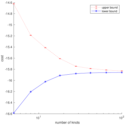
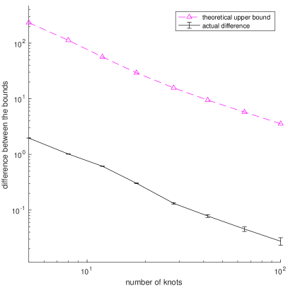
Figure 4.1. Results from the numerical example. Left: upper and lower bounds on (MMOT) resulted from Algorithm 2 (i.e., $\mathsf{MMOT}^{\mathsf{U}\mathsf{B}}$ and $\mathsf{MMOT}^{\mathsf{L}\mathsf{B}}$) plotted against the number of knots in each dimension (i.e., $m_{i}+1$). The error bars around the upper bounds mark the 95% Monte Carlo error bounds. Right: theoretical upper bounds on $\mathsf{MMOT}^{\mathsf{U}\mathsf{B}}-\mathsf{MMOT}^{\mathsf{L}\mathsf{B}}$ versus the actual differences resulted from computation. The error bars around the actual gaps mark the 95% Monte Carlo error bounds.

The results in this experiment are shown in Figure 4.1. The left panel of Figure 4.1 shows the values of $\mathsf{MMOT}^{\mathsf{L}\mathsf{B}}$ and $\mathsf{MMOT}^{\mathsf{U}\mathsf{B}}$ as the number of knots increases from 5 to 100. Since $\mathsf{MMOT}^{\mathsf{U}\mathsf{B}}$ was approximated by Monte Carlo integration, we have plotted the 95% Monte Carlo error bounds around the estimated values of $\mathsf{MMOT}^{\mathsf{U}\mathsf{B}}$. It can be observed that both $\mathsf{MMOT}^{\mathsf{L}\mathsf{B}}$ and $\mathsf{MMOT}^{\mathsf{U}\mathsf{B}}$ improved drastically when the number of knots increased from 5 to 18. After that, when more knots were added, the improvements in $\mathsf{MMOT}^{\mathsf{L}\mathsf{B}}$ and $\mathsf{MMOT}^{\mathsf{U}\mathsf{B}}$ both shrunk. When 100 knots were used, the difference between $\mathsf{MMOT}^{\mathsf{U}\mathsf{B}}$ and $\mathsf{MMOT}^{\mathsf{L}\mathsf{B}}$ was around $0.027$. This shows that with 100 knots the approximate optimizer $\tilde{\mu}$ of (MMOT) returned by Algorithm 2 was close to being optimal. The right panel of Figure 4.1 compares the differences between $\mathsf{MMOT}^{\mathsf{U}\mathsf{B}}$ and $\mathsf{MMOT}^{\mathsf{L}\mathsf{B}}$ computed by Algorithm 2 with their theoretical upper bounds. These theoretical upper bounds on the gaps were computed based on (4.1) and upper bounds on $\overline{W}_{1,\mu_{i}}\big{(}[\mu_{i}]_{\mathcal{G}_{i}}\big{)}$ for $i=1,\ldots,N$. One can observe that the actual differences are about two orders of magnitude smaller than their theoretical upper bounds. This shows that despite our theoretical analysis of Algorithm 2 in Theorem 4.2.3 requiring $\eta(\mathfrak{C}_{i})\leq\frac{\tilde{\epsilon}-\epsilon}{2NL_{f}}$ for $i=1,\ldots,N$ in order to guarantee $\mathsf{MMOT}^{\mathsf{U}\mathsf{B}}-\mathsf{MMOT}^{\mathsf{L}\mathsf{B}}\leq\tilde{\epsilon}$, the actual difference between $\mathsf{MMOT}^{\mathsf{U}\mathsf{B}}$ and $\mathsf{MMOT}^{\mathsf{L}\mathsf{B}}$ is likely much smaller than $\tilde{\epsilon}$ in practice. This also means that one may use much fewer knots in practice than what the theoretical analysis suggests.

5. Proof of theoretical results

5.1. Proof of results in Section 2.2

Proof of Lemma 2.2.3.

Let $\hat{\mu}_{1},\ldots,\hat{\mu}_{N}$ denote the marginals of $\hat{\mu}$ on $\mathcal{X}_{1},\ldots,\mathcal{X}_{N}$, respectively. Since $\hat{\mu}\in\mathcal{P}_{1}({\bm{\mathcal{X}}})$, we have $\hat{\mu}_{i}\in\mathcal{P}_{1}(\mathcal{X}_{i})$ for $i=1,\ldots,N$ by (2.3). Moreover, the existence of an optimal coupling $\gamma_{i}$ of $\hat{\mu}_{i}$ and $\mu_{i}$ under the cost function $d_{\mathcal{X}_{i}}$ follows from [64, Theorem 4.1], $d_{\mathcal{X}_{i}}\geq 0$, and the continuity of $d_{\mathcal{X}_{i}}$. The existence of a probability measure $\gamma\in\mathcal{P}(\mathcal{X}_{1}\times\cdots\times\mathcal{X}_{N}\times\bar{\mathcal{X}}_{1}\times\cdots\times\bar{\mathcal{X}}_{N})$ that satisfies the conditions in Definition 2.2.2 follows from the following inductive argument that repeatedly applies Lemma 2.2.1. Specifically, one first applies Lemma 2.2.1 with $\mathcal{Y}_{1}\leftarrow\mathcal{X}_{2}\times\cdots\times\mathcal{X}_{N}$, $\mathcal{Y}_{2}\leftarrow\mathcal{X}_{1}$, $\mathcal{Y}_{3}\leftarrow\bar{\mathcal{X}}_{1}$ to “glue together” $\hat{\mu}$ and $\gamma_{1}$ and obtain $\gamma^{(1)}\in\mathcal{P}(\mathcal{X}_{1}\times\cdots\times\mathcal{X}_{N}\times\bar{\mathcal{X}}_{1})$. Subsequently, for $i=2,\ldots,N$, one applies Lemma 2.2.1 with $\mathcal{Y}_{1}\leftarrow\Big{(}{}_{j=1,\ldots,N,j\neq i}\mathcal{X}_{j}\Big{)}\times\Big{(}{}_{k=1,\ldots,i-1}\bar{\mathcal{X}}_{k}\Big{)}$, $\mathcal{Y}_{2}\leftarrow\mathcal{X}_{i}$, $\mathcal{Y}_{3}\leftarrow\bar{\mathcal{X}}_{i}$ to “glue together” $\gamma^{(i-1)}$ and $\gamma_{i}$ and obtain $\gamma^{(i)}\in\mathcal{P}(\mathcal{X}_{1}\times\cdots\times\mathcal{X}_{N}\times\bar{\mathcal{X}}_{1}\times\cdots\times\bar{\mathcal{X}}_{i})$. One may check that $\gamma^{(N)}$ satisfies all the required properties of $\gamma$ and thus letting $\gamma:=\gamma^{(N)}$ completes the construction. Finally, one may check that the marginal $\tilde{\mu}$ of $\gamma$ on $\bar{\mathcal{X}}_{1}\times\cdots\times\bar{\mathcal{X}}_{N}$ satisfies $\tilde{\mu}\in R(\hat{\mu};\mu_{1},\ldots,\mu_{N})$. ∎

Proof of Proposition 2.2.7.

Let us first prove statement (i). Let us fix an arbitrary $\epsilon>0$ and an arbitrary $\epsilon$-optimal solution $\mu_{\epsilon}\in\Gamma\big{(}[\mu_{1}]_{\mathcal{G}_{1}},\ldots,[\mu_{N}]_{\mathcal{G}_{N}}\big{)}$ of ($\textsf{MMOT}_{\textsf{relax}}$). Let us denote $\beta:=\int_{{\bm{\mathcal{X}}}}f\,\mathrm{d}{\mu_{\epsilon}}$. We thus have $\beta\leq\inf_{\mu\in\Gamma([\mu_{1}]_{\mathcal{G}_{1}},\ldots,[\mu_{N}]_{\mathcal{G}_{N}})}\Big{\{}\int_{{\bm{\mathcal{X}}}}f\,\mathrm{d}{\mu}\Big{\}}+\epsilon$. Let ${\bm{\phi}}:{\bm{\mathcal{X}}}\to\mathbb{R}^{m+2}$ be given by

$${\bm{\phi}}(x_{1},\ldots,x_{N}) :=\big{(}1,g_{1,1}(x_{1}),\ldots,g_{1,m_{1}}(x_{1}),\ldots,g_{N,1}(x_{N}),\ldots,g_{N,m_{N}}(x_{N}),f(x_{1},\ldots,x_{N})\big{)}^{\mathsf{T}}$$

$$\hskip 290.0pt\forall(x_{1},\ldots,x_{N})\in{\bm{\mathcal{X}}}.$$

By an application of Tchakaloff’s theorem in [6, Corollary 2], there exist $q\in\mathbb{N}$, $\alpha_{1}>0,\ldots,\alpha_{q}>0$, ${\bm{x}}_{1}\in{\bm{\mathcal{X}}},\ldots,{\bm{x}}_{q}\in{\bm{\mathcal{X}}}$ with $1\leq q\leq m+2$, such that

$$\sum_{k=1}^{q}\alpha_{k} =\int_{{\bm{\mathcal{X}}}}1\,\mathrm{d}{\mu_{\epsilon}}=1,$$ (5.1)

$$\sum_{k=1}^{q}\alpha_{k}g_{i,j}(\pi_{i}({\bm{x}}_{k})) =\int_{{\bm{\mathcal{X}}}}g_{i,j}\circ\pi_{i}\,\mathrm{d}{\mu_{\epsilon}}=\int_{\mathcal{X}_{i}}g_{i,j}\,\mathrm{d}{\mu_{i}}\qquad\forall 1\leq j\leq m_{i},\;\forall 1\leq i\leq N,$$ (5.2)

$$\sum_{k=1}^{q}\alpha_{k}f({\bm{x}}_{k}) =\int_{{\bm{\mathcal{X}}}}f\,\mathrm{d}{\mu_{\epsilon}}=\beta\leq\inf_{\mu\in\Gamma([\mu_{1}]_{\mathcal{G}_{1}},\ldots,[\mu_{N}]_{\mathcal{G}_{N}})}\bigg{\{}\int_{{\bm{\mathcal{X}}}}f\,\mathrm{d}{\mu}\bigg{\}}+\epsilon.$$ (5.3)

Let $\hat{\mu}:=\sum_{k=1}^{q}\alpha_{k}\delta_{{\bm{x}}_{k}}$. Then, it follows from (5.1) that $\hat{\mu}\in\mathcal{P}({\bm{\mathcal{X}}})$. For $i=1,\ldots,N$, let us denote the marginal of $\hat{\mu}$ on $\mathcal{X}_{i}$ by $\hat{\mu}_{i}$. Subsequently, (5.2) guarantees that $\int_{\mathcal{X}_{i}}g_{i,j}\,\mathrm{d}{\hat{\mu}_{i}}=\int_{{\bm{\mathcal{X}}}}{g_{i,j}\circ\pi_{i}}\,\mathrm{d}{\hat{\mu}}=\sum_{k=1}^{q}\alpha_{k}g_{i,j}(\pi_{i}({\bm{x}}_{k}))=\int_{\mathcal{X}_{i}}g_{i,j}\,\mathrm{d}{\mu_{i}}$ for $j=1,\ldots,m_{i}$, $i=1,\ldots,N$ and it hence holds that $\hat{\mu}\in\Gamma\big{(}[\mu_{1}]_{\mathcal{G}_{1}},\ldots,[\mu_{N}]_{\mathcal{G}_{N}}\big{)}$. Finally, (5.3) implies that

$$\int_{{\bm{\mathcal{X}}}}f\,\mathrm{d}{\hat{\mu}}=\sum_{k=1}^{q}\alpha_{k}f({\bm{x}}_{k})\leq\inf_{\mu\in\Gamma([\mu_{1}]_{\mathcal{G}_{1}},\ldots,[\mu_{N}]_{\mathcal{G}_{N}})}\bigg{\{}\int_{{\bm{\mathcal{X}}}}f\,\mathrm{d}{\mu}\bigg{\}}+\epsilon,$$

showing that $\hat{\mu}$ is an $\epsilon$-optimal solution of ($\textsf{MMOT}_{\textsf{relax}}$). This proves statement (i). To prove statement (ii), observe that when $\mathcal{X}_{1},\ldots,\mathcal{X}_{N}$ are compact and all test functions $(g_{i,j})_{j=1:m_{i},i=1:N}$ are continuous, an optimizer $\mu^{\star}$ of ($\textsf{MMOT}_{\textsf{relax}}$) is attained since $\Gamma\big{(}[\mu_{1}]_{\mathcal{G}_{1}},\ldots,[\mu_{N}]_{\mathcal{G}_{N}}\big{)}$ is a closed subset of the compact metric space $\big{(}\mathcal{P}({\bm{\mathcal{X}}}),W_{1}\big{)}$ (see, e.g., [64, Remark 6.19]) and the mapping $\mathcal{P}({\bm{\mathcal{X}}})\ni\mu\mapsto\int_{{\bm{\mathcal{X}}}}f\,\mathrm{d}{\mu}\in\mathbb{R}$ is lower semi-continuous (see, e.g., [64, Lemma 4.3]). The statement then follows from the same argument used in the proof of statement (i) with $\mu_{\epsilon}$ replaced by $\mu^{\star}$. The proof is now complete. ∎

Proof of Theorem 2.2.9.

To prove statement (i), let us split the left-hand side of the inequality into two parts:

$$\int_{{\bm{\mathcal{X}}}}f\,\mathrm{d}{\tilde{\mu}}-\int_{{\bm{\mathcal{X}}}}f\,\mathrm{d}{\hat{\mu}}=\left(\int_{D}f\,\mathrm{d}{\tilde{\mu}}-\int_{D}f\,\mathrm{d}{\hat{\mu}}\right)+\left(\int_{{\bm{\mathcal{X}}}\setminus D}f\,\mathrm{d}{\tilde{\mu}}-\int_{{\bm{\mathcal{X}}}\setminus D}f\,\mathrm{d}{\hat{\mu}}\right)$$ (5.4)

and control them separately. By the assumption that $\tilde{\mu}\in R(\hat{\mu};\mu_{1},\ldots,\mu_{N})$ and Definition 2.2.2, there exists a probability measure $\gamma\in\mathcal{P}(\mathcal{X}_{1}\times\cdots\times\mathcal{X}_{N}\times\bar{\mathcal{X}}_{1}\times\cdots\times\bar{\mathcal{X}}_{N})$, such that the marginal of $\gamma$ on $\mathcal{X}_{1}\times\cdots\times\mathcal{X}_{N}$ is $\hat{\mu}$, the marginal $\gamma_{i}\in\Gamma(\hat{\mu}_{i},\mu_{i})$ of $\gamma$ on $\mathcal{X}_{i}\times\bar{\mathcal{X}}_{i}$ satisfies $\int_{\mathcal{X}_{i}\times\bar{\mathcal{X}}_{i}}d_{\mathcal{X}_{i}}(x,y)\,{\gamma_{i}}\!\left({\mathrm{d}x,\mathrm{d}y}\right)\!=W_{1}(\hat{\mu}_{i},\mu_{i})$ for $i=1,\ldots,N$, and the marginal of $\gamma$ on $\bar{\mathcal{X}}_{1}\times\cdots\times\bar{\mathcal{X}}_{N}$ is $\tilde{\mu}$. Thus, we have by (2.3) that

$$\begin{split}\int_{D}f\,\mathrm{d}{\tilde{\mu}}-\int_{D}f\,\mathrm{d}{\hat{\mu}}&=\int_{D\times D}f(\bar{x}_{1},\ldots,\bar{x}_{N})-f(x_{1},\ldots,x_{N})\,{\gamma}\!\left({\mathrm{d}x_{1},\ldots,\mathrm{d}x_{N},\mathrm{d}\bar{x}_{1},\ldots,\mathrm{d}\bar{x}_{N}}\right)\!\\ &\leq\int_{D\times D}L_{f}d_{{\bm{\mathcal{X}}}}\big{(}(x_{1},\ldots,x_{N}),(\bar{x}_{1},\ldots,\bar{x}_{N})\big{)}\,{\gamma}\!\left({\mathrm{d}x_{1},\ldots,\mathrm{d}x_{N},\mathrm{d}\bar{x}_{1},\ldots,\mathrm{d}\bar{x}_{N}}\right)\!\\ &\leq\int_{{\bm{\mathcal{X}}}\times{\bm{\mathcal{X}}}}L_{f}d_{{\bm{\mathcal{X}}}}\big{(}(x_{1},\ldots,x_{N}),(\bar{x}_{1},\ldots,\bar{x}_{N})\big{)}\,{\gamma}\!\left({\mathrm{d}x_{1},\ldots,\mathrm{d}x_{N},\mathrm{d}\bar{x}_{1},\ldots,\mathrm{d}\bar{x}_{N}}\right)\!\\ &=L_{f}\int_{{\bm{\mathcal{X}}}\times{\bm{\mathcal{X}}}}\sum_{i=1}^{N}d_{\mathcal{X}_{i}}(x_{i},\bar{x}_{i})\,{\gamma}\!\left({\mathrm{d}x_{1},\ldots,\mathrm{d}x_{N},\mathrm{d}\bar{x}_{1},\ldots,\mathrm{d}\bar{x}_{N}}\right)\!\\ &=\sum_{i=1}^{N}L_{f}\int_{\mathcal{X}_{i}\times\mathcal{X}_{i}}d_{\mathcal{X}_{i}}(x_{i},\bar{x}_{i})\,{\gamma_{i}}\!\left({\mathrm{d}x_{i},\mathrm{d}\bar{x}_{i}}\right)\!\\ &=\sum_{i=1}^{N}L_{f}W_{1}(\mu_{i},\hat{\mu}_{i}).\end{split}$$ (5.5)

Moreover, by the assumption that $\hat{\mu}_{i}\in[\mu_{i}]_{\mathcal{G}_{i}}$ and $\underline{f}_{i}\in\mathrm{span}_{1}(\mathcal{G}_{i})$ for $i=1,\ldots,N$, we have

$$\begin{split}\int_{{\bm{\mathcal{X}}}\setminus D}f\,\mathrm{d}{\tilde{\mu}}-\int_{{\bm{\mathcal{X}}}\setminus D}f\,\mathrm{d}{\hat{\mu}}&\leq\int_{{\bm{\mathcal{X}}}}\left(\sum_{i=1}^{N}\overline{f}_{i}\circ\pi_{i}\right)\,\mathrm{d}{\tilde{\mu}}-\int_{{\bm{\mathcal{X}}}}\left(\sum_{i=1}^{N}\underline{f}_{i}\circ\pi_{i}\right)\,\mathrm{d}{\hat{\mu}}\\ &=\sum_{i=1}^{N}\left(\int_{\mathcal{X}_{i}}\overline{f}_{i}\,\mathrm{d}{\mu_{i}}-\int_{\mathcal{X}_{i}}\underline{f}_{i}\,\mathrm{d}{\hat{\mu}_{i}}\right)\\ &=\sum_{i=1}^{N}\int_{\mathcal{X}_{i}}\overline{f}_{i}-\underline{f}_{i}\,\mathrm{d}{\mu_{i}}.\end{split}$$ (5.6)

Subsequently, combining (5.4), (5.5), and (5.6) proves statement (i).

To prove statement (ii), observe that for any ${\bm{x}}=(x_{1},\ldots,x_{N})\in{\bm{\mathcal{X}}}$, since $(\hat{x}_{1},\ldots,\hat{x}_{N})\in D$, we obtain

$$\begin{split}f({\bm{x}})&=f({\bm{x}})\mathbbm{1}_{D}({\bm{x}})+f({\bm{x}})\mathbbm{1}_{{\bm{\mathcal{X}}}\setminus D}({\bm{x}})\\ &\geq-\big{|}f(\hat{x}_{1},\ldots,\hat{x}_{N})\big{|}-L_{f}\left(\sum_{i=1}^{N}d_{\mathcal{X}_{i}}(x_{i},\hat{x}_{i})\right)+\left(\sum_{i=1}^{N}\underline{f}_{i}(x_{i})\right)\\ &\geq-\big{|}f(\hat{x}_{1},\ldots,\hat{x}_{N})\big{|}-L_{f}\left(\sum_{i=1}^{N}h_{i}(x_{i})\right)+\left(\sum_{i=1}^{N}\underline{f}_{i}(x_{i})\right).\end{split}$$ (5.7)

Thus, for any $\hat{\mu}\in\Gamma\big{(}[\mu_{1}]_{\mathcal{G}_{1}},\ldots,[\mu_{N}]_{\mathcal{G}_{N}}\big{)}$, we have

$$\int_{{\bm{\mathcal{X}}}}f\,\mathrm{d}{\hat{\mu}} \geq-\big{|}f(\hat{x}_{1},\ldots,\hat{x}_{N})\big{|}-L_{f}\left(\sum_{i=1}^{N}\int_{{\bm{\mathcal{X}}}}h_{i}\circ\pi_{i}\,\mathrm{d}{\hat{\mu}}\right)+\sum_{i=1}^{N}\int_{{\bm{\mathcal{X}}}}\underline{f}_{i}\circ\pi_{i}\,\mathrm{d}{\hat{\mu}}$$

$$=-\big{|}f(\hat{x}_{1},\ldots,\hat{x}_{N})\big{|}-L_{f}\left(\sum_{i=1}^{N}\int_{\mathcal{X}_{i}}h_{i}\,\mathrm{d}{\mu_{i}}\right)+\sum_{i=1}^{N}\int_{\mathcal{X}_{i}}\underline{f}_{i}\,\mathrm{d}{\mu_{i}}>-\infty,$$

which does not depend on $\hat{\mu}$. This proves statement (ii).

To prove statement (iii), let us fix an arbitrary $i\in\{1,\ldots,N\}$. For any $\nu_{i}\in[\mu_{i}]_{\mathcal{G}_{i}}$, it holds that

$$W_{1}(\mu_{i},\nu_{i}) \leq W_{1}(\mu_{i},\delta_{\hat{x}_{i}})+W_{1}(\nu_{i},\delta_{\hat{x}_{i}})$$

$$=W_{1}(\mu_{i},\delta_{\hat{x}_{i}})+\int_{\mathcal{X}_{i}}d_{\mathcal{X}_{i}}(\hat{x}_{i},x)\,{\nu_{i}}\!\left({\mathrm{d}x}\right)\!$$

$$\leq W_{1}(\mu_{i},\delta_{\hat{x}_{i}})+\int_{\mathcal{X}_{i}}h_{i}(x)\,{\nu_{i}}\!\left({\mathrm{d}x}\right)\!$$

$$=W_{1}(\mu_{i},\delta_{\hat{x}_{i}})+\int_{\mathcal{X}_{i}}h_{i}(x)\,{\mu_{i}}\!\left({\mathrm{d}x}\right)\!$$

$$<\infty.$$

Thus, $\overline{W}_{1,\mu_{i}}([\mu_{i}]_{\mathcal{G}_{i}})=\sup_{\nu_{i}\in[\mu_{i}]_{\mathcal{G}_{i}}}\big{\{}W_{1}(\mu_{i},\nu_{i})\big{\}}\leq W_{1}(\mu_{i},\delta_{\hat{x}_{i}})+\int_{\mathcal{X}}h_{i}(x)\,{\mu_{i}}\!\left({\mathrm{d}x}\right)\!<\infty$, which proves statement (iii).

Let us now prove statement (iv). For $i=1,\ldots,N$, let $\hat{\mu}_{i}\in\mathcal{P}_{1}(\mathcal{X}_{i})$ denote the marginal of $\hat{\mu}$ on $\mathcal{X}_{i}$. We have $\hat{\mu}_{i}\in[\mu_{i}]_{\mathcal{G}_{i}}$ by the definition of $\Gamma\big{(}[\mu_{1}]_{\mathcal{G}_{1}},\ldots,[\mu_{N}]_{\mathcal{G}_{N}}\big{)}$. By statement (i), we have

$$\begin{split}\int_{{\bm{\mathcal{X}}}}f\,\mathrm{d}{\tilde{\mu}}-\int_{{\bm{\mathcal{X}}}}f\,\mathrm{d}{\hat{\mu}}&\leq\sum_{i=1}^{N}\left(L_{f}W_{1}(\mu_{i},\hat{\mu}_{i})+\int_{\mathcal{X}_{i}}\overline{f}_{i}-\underline{f}_{i}\,\mathrm{d}{\mu_{i}}\right)\\ &\leq\sum_{i=1}^{N}\left(L_{f}\overline{W}_{1,\mu_{i}}([\mu_{i}]_{\mathcal{G}_{i}})+\int_{\mathcal{X}_{i}}\overline{f}_{i}-\underline{f}_{i}\,\mathrm{d}{\mu_{i}}\right).\end{split}$$ (5.8)

Moreover, since by definition $\mu_{i}\in[\mu_{i}]_{\mathcal{G}_{i}}$ for $i=1,\ldots,N$, we have $\Gamma(\mu_{1},\ldots,\mu_{N})\subseteq\Gamma\big{(}[\mu_{1}]_{\mathcal{G}_{1}},$ $\ldots,$ $[\mu_{N}]_{\mathcal{G}_{N}}\big{)}$. Hence,

$$\inf_{\mu\in\Gamma([\mu_{1}]_{\mathcal{G}_{1}},\ldots,[\mu_{N}]_{\mathcal{G}_{N}})}\bigg{\{}\int_{{\bm{\mathcal{X}}}}f\,\mathrm{d}{\mu}\bigg{\}}\leq\inf_{\mu\in\Gamma(\mu_{1},\ldots,\mu_{N})}\bigg{\{}\int_{{\bm{\mathcal{X}}}}f\,\mathrm{d}{\mu}\bigg{\}}.$$ (5.9)

We then combine (5.8), (2.9), and (5.9) to finish the proof of statement (iv).

Finally, let us prove statement (v). The first inequality in (2.10) follows from (5.9). Moreover, for every $\hat{\mu}\in\Gamma\big{(}[\mu_{1}]_{\mathcal{G}_{1}},\ldots,[\mu_{N}]_{\mathcal{G}_{N}}\big{)}$ and every $\tilde{\mu}\in R(\hat{\mu};\mu_{1},\ldots,\mu_{N})\subset\Gamma(\mu_{1},\ldots,\mu_{N})$, we have by (5.8) that

$$\inf_{\mu\in\Gamma(\mu_{1},\ldots,\mu_{N})}\bigg{\{}\int_{{\bm{\mathcal{X}}}}f\,\mathrm{d}{\mu}\bigg{\}}-\int_{{\bm{\mathcal{X}}}}f\,\mathrm{d}{\hat{\mu}} \leq\int_{{\bm{\mathcal{X}}}}f\,\mathrm{d}{\tilde{\mu}}-\int_{{\bm{\mathcal{X}}}}f\,\mathrm{d}{\hat{\mu}}$$

$$\leq\sum_{i=1}^{N}\left(L_{f}\overline{W}_{1,\mu_{i}}([\mu_{i}]_{\mathcal{G}_{i}})+\int_{\mathcal{X}_{i}}\overline{f}_{i}-\underline{f}_{i}\,\mathrm{d}{\mu_{i}}\right)<\infty.$$

By taking the infimum over $\hat{\mu}\in\Gamma\big{(}[\mu_{1}]_{\mathcal{G}_{1}},\ldots,[\mu_{N}]_{\mathcal{G}_{N}}\big{)}$ in the inequality above, we conclude that the second inequality in (2.10) holds. The proof is now complete. ∎

Proof of Theorem 2.2.11.

By a multi-marginal extension of [64, Lemma 4.4], one can show that $\Gamma(\mu_{1},\ldots,\mu_{N})$ is weakly precompact. Hence, $\big{(}\tilde{\mu}^{(l)}\big{)}_{l\in\mathbb{N}}$ has at least one weakly convergent subsequence. Now, assume without loss of generality that $\tilde{\mu}^{(l)}$ converges weakly to $\tilde{\mu}$ as $l\to\infty$, where $\tilde{\mu}\in\mathcal{P}({\bm{\mathcal{X}}})$. For $i=1,\ldots,N$ and for any bounded continuous function $h:\mathcal{X}_{i}\to\mathbb{R}$, we have

$$\int_{{\bm{\mathcal{X}}}}h\circ\pi_{i}\,\mathrm{d}{\tilde{\mu}}=\lim_{l\to\infty}\int_{{\bm{\mathcal{X}}}}h\circ\pi_{i}\,\mathrm{d}{\tilde{\mu}^{(l)}}=\int_{\mathcal{X}_{i}}h\,\mathrm{d}{\mu_{i}}.$$

Thus, $\tilde{\mu}\in\Gamma(\mu_{1},\ldots,\mu_{N})$. Moreover, for any $\hat{{\bm{x}}}=(\hat{x}_{1},\ldots,\hat{x}_{N})\in{\bm{\mathcal{X}}}$, we have

$$\lim_{l\to\infty}\int_{{\bm{\mathcal{X}}}}d_{{\bm{\mathcal{X}}}}(\hat{{\bm{x}}},{\bm{x}})\,{\tilde{\mu}^{(l)}}\!\left({\mathrm{d}{\bm{x}}}\right)\!=\sum_{i=1}^{N}\int_{\mathcal{X}_{i}}d_{\mathcal{X}_{i}}(\hat{x}_{i},x)\,{\mu_{i}}\!\left({\mathrm{d}x}\right)\!=\int_{{\bm{\mathcal{X}}}}d_{{\bm{\mathcal{X}}}}(\hat{{\bm{x}}},{\bm{x}})\,{\tilde{\mu}}\!\left({\mathrm{d}{\bm{x}}}\right)\!.$$

Therefore, we have by [64, Definition 6.8] and [64, Theorem 6.9] that $\tilde{\mu}^{(l)}\to\tilde{\mu}$ in $\big{(}\mathcal{P}_{1}({\bm{\mathcal{X}}}),W_{1}\big{)}$ as $l\to\infty$. By (5.8), we have for every $l\in\mathbb{N}$ that

$$\int_{{\bm{\mathcal{X}}}}f\,\mathrm{d}{\tilde{\mu}^{(l)}}\leq\int_{{\bm{\mathcal{X}}}}f\,\mathrm{d}{\hat{\mu}^{(l)}}+\sum_{i=1}^{N}\left(L^{(l)}_{f}\overline{W}_{1,\mu_{i}}\left([\mu_{i}]_{\mathcal{G}^{(l)}_{i}}\right)+\int_{\mathcal{X}_{i}}\overline{f}^{(l)}_{i}-\underline{f}^{(l)}_{i}\,\mathrm{d}{\mu_{i}}\right).$$

Thus, for every $l\in\mathbb{N}$, we have by (2.11) and Theorem 2.2.9(iv) that

$$\inf_{\mu\in\Gamma(\mu_{1},\ldots,\mu_{N})}\bigg{\{}\int_{{\bm{\mathcal{X}}}}f\,\mathrm{d}{\mu}\bigg{\}} \geq\int_{{\bm{\mathcal{X}}}}f\,\mathrm{d}{\tilde{\mu}^{(l)}}-\left(\sum_{i=1}^{N}L^{(l)}_{f}\overline{W}_{1,\mu_{i}}\left([\mu_{i}]_{\mathcal{G}^{(l)}_{i}}\right)+\int_{\mathcal{X}_{i}}\overline{f}^{(l)}_{i}-\underline{f}^{(l)}_{i}\,\mathrm{d}{\mu_{i}}\right)-\epsilon^{(l)}.$$

Moreover, by Assumption 2.1.3 and a multi-marginal extension of [64, Lemma 4.3], we have $\liminf_{l\to\infty}\big{\{}\int_{{\bm{\mathcal{X}}}}f\,\mathrm{d}{\tilde{\mu}^{(l)}}\big{\}}\geq\int_{{\bm{\mathcal{X}}}}f\,\mathrm{d}{\tilde{\mu}}$. Hence,

$$\int_{{\bm{\mathcal{X}}}}f\,\mathrm{d}{\tilde{\mu}} \geq\inf_{\mu\in\Gamma(\mu_{1},\ldots,\mu_{N})}\bigg{\{}\int_{{\bm{\mathcal{X}}}}f\,\mathrm{d}{\mu}\bigg{\}}$$

$$\geq\liminf_{l\to\infty}\left[\int_{{\bm{\mathcal{X}}}}f\,\mathrm{d}{\tilde{\mu}^{(l)}}-\left(\sum_{i=1}^{N}L^{(l)}_{f}\overline{W}_{1,\mu_{i}}\left([\mu_{i}]_{\mathcal{G}^{(l)}_{i}}\right)+\int_{\mathcal{X}_{i}}\overline{f}^{(l)}_{i}-\underline{f}^{(l)}_{i}\,\mathrm{d}{\mu_{i}}\right)-\epsilon^{(l)}\right]$$

$$\geq\int_{{\bm{\mathcal{X}}}}f\,\mathrm{d}{\tilde{\mu}}.$$

This shows that $\tilde{\mu}$ is an optimizer of (MMOT). The proof is now complete. ∎

5.2. Proof of results in Section 2.3

Proof of Theorem 2.3.1.

For any $y_{0}\in\mathbb{R}$ and ${\bm{y}}\in\mathbb{R}^{m}$ such that $y_{0}+\langle{\bm{g}}({\bm{x}}),{\bm{y}}\rangle\leq f({\bm{x}})$ $\forall{\bm{x}}\in{\bm{\mathcal{X}}}$, and any $\mu\in\Gamma\big{(}[\mu_{1}]_{\mathcal{G}_{1}},\ldots,[\mu_{N}]_{\mathcal{G}_{N}}\big{)}$, it holds that

$$y_{0}+\langle{\bm{v}},{\bm{y}}\rangle=\int_{{\bm{\mathcal{X}}}}y_{0}+\langle{\bm{g}}({\bm{x}}),{\bm{y}}\rangle\,{\mu}\!\left({\mathrm{d}{\bm{x}}}\right)\!\leq\int_{{\bm{\mathcal{X}}}}f({\bm{x}})\,{\mu}\!\left({\mathrm{d}{\bm{x}}}\right)\!.$$ (5.10)

Taking the supremum over all such $y_{0}\in\mathbb{R}$ and ${\bm{y}}\in\mathbb{R}^{m}$ and taking the infimum over all $\mu\in\Gamma([\mu_{1}]_{\mathcal{G}_{1}},\ldots$, $[\mu_{N}]_{\mathcal{G}_{N}})$ yields the weak duality (2.14). This proves statement (i).

Now, to establish the strong duality, we assume that the left-hand side of (2.14) is not $-\infty$. We first show that ${\bm{v}}\in\mathrm{cl}(K)$. Suppose, for the sake of contradiction, that ${\bm{v}}\notin\mathrm{cl}(K)$. Then, due to strong separation (see, e.g., [55, Corollary 11.4.2]), there exist ${\bm{y}}\in\mathbb{R}^{m}$ and $\alpha>0$ such that $\langle{\bm{w}},{\bm{y}}\rangle-\langle{\bm{v}},{\bm{y}}\rangle\geq\alpha$ for all ${\bm{w}}\in\mathrm{cl}(K)$. In particular, we have $\langle{\bm{g}}({\bm{x}}),{\bm{y}}\rangle-\langle{\bm{v}},{\bm{y}}\rangle\geq\alpha$ for all ${\bm{x}}\in{\bm{\mathcal{X}}}$. However, this implies that for any $\mu\in\Gamma(\mu_{1},\ldots,\mu_{N})$, we have

$$0=\langle{\bm{v}},{\bm{y}}\rangle-\langle{\bm{v}},{\bm{y}}\rangle=\int_{{\bm{\mathcal{X}}}}\langle{\bm{g}}({\bm{x}}),{\bm{y}}\rangle-\langle{\bm{v}},{\bm{y}}\rangle\,{\mu}\!\left({\mathrm{d}{\bm{x}}}\right)\!\geq\alpha>0,$$

which is a contradiction. This shows that ${\bm{v}}\in\mathrm{cl}(K)$.

Next, to prove statement (ii), let us first suppose that the condition (SD1) holds, i.e., ${\bm{v}}\in\mathrm{relint}(K)$. Let $U:=\mathrm{cone}\Big{(}\Big{\{}(1,{\bm{g}}({\bm{x}})^{\mathsf{T}})^{\mathsf{T}}:{\bm{x}}\in{\bm{\mathcal{X}}}\Big{\}}\Big{)}=\mathrm{cone}\Big{(}\Big{\{}(1,{\bm{u}}^{\mathsf{T}})^{\mathsf{T}}:{\bm{u}}\in K\Big{\}}\Big{)}\subset\mathbb{R}^{m+1}$. By [55, Corollary 6.8.1], it holds that

$$\mathrm{relint}(U)=\big{\{}(\lambda,\lambda{\bm{u}}^{\mathsf{T}})^{\mathsf{T}}:\lambda>0,\;{\bm{u}}\in\mathrm{relint}(K)\big{\}}.$$ (5.11)

Under the assumption that ${\bm{v}}\in\mathrm{relint}(K)$, we have $(1,{\bm{v}}^{\mathsf{T}})^{\mathsf{T}}\in\mathrm{relint}(U)$, and thus by [38, Theorem 8.2] (see the fifth case in [38, Table 8.1]), with $M\leftarrow U$, $N\leftarrow C$, $K\leftarrow\mathrm{cone}\Big{(}C\cup\big{\{}(\mathbf{0}_{m+1}^{\mathsf{T}},1)^{\mathsf{T}}\big{\}}\Big{)}$, $c\leftarrow(1,{\bm{v}}^{\mathsf{T}})^{\mathsf{T}}$ in the notation of [38] (see also [38, p. 81 & p. 49]), the left-hand side of (2.14) coincides with the optimal value of the following problem:

$$\begin{split}\operatorname*{\mathrm{minimize}}_{(a_{l},{\bm{x}}_{l})}\quad&\sum_{l=1}^{k}\alpha_{l}f({\bm{x}}_{l})\\ \text{subject to}\quad&\sum_{l=1}^{k}\alpha_{l}=1,\\ &\sum_{l=1}^{k}\alpha_{l}{\bm{g}}({\bm{x}}_{l})={\bm{v}},\\ &k\in\mathbb{N},\;(\alpha_{l})_{l=1:k}\subset\mathbb{R}_{+},\;({\bm{x}}_{l})_{l=1:k}\subset{\bm{\mathcal{X}}}.\end{split}$$ (5.12)

Notice that for any $(\alpha_{l})_{l=1:k}\subset\mathbb{R}_{+}$, $({\bm{x}}_{l})_{l=1:k}\subset{\bm{\mathcal{X}}}$ that is feasible for problem (5.12), it holds by (2.12) and (2.13) that $\hat{\mu}:=\sum_{l=1}^{k}\alpha_{l}\delta_{{\bm{x}}_{l}}$ is a positive Borel measure which satisfies

$$\hat{\mu}({\bm{\mathcal{X}}}) =\sum_{l=1}^{k}\alpha_{l}=1,$$

$$\int_{{\bm{\mathcal{X}}}}g_{i,j}\circ\pi_{i}\,\mathrm{d}{\hat{\mu}} =\sum_{l=1}^{k}\alpha_{l}g_{i,j}\circ\pi_{i}({\bm{x}}_{l})=\int_{\mathcal{X}_{i}}g_{i,j}\,\mathrm{d}{\mu_{i}}\qquad\qquad\forall 1\leq j\leq m_{i},\;\forall 1\leq i\leq N.$$

This shows that $\hat{\mu}\in\Gamma\big{(}[\mu_{1}]_{\mathcal{G}_{1}},\ldots,[\mu_{N}]_{\mathcal{G}_{N}}\big{)}$. Moreover, since $\int_{{\bm{\mathcal{X}}}}f\,\mathrm{d}{\hat{\mu}}=\sum_{l=1}^{k}\alpha_{l}f({\bm{x}}_{l})$, it holds that $\inf_{\mu\in\Gamma([\mu_{1}]_{\mathcal{G}_{1}},\ldots,[\mu_{N}]_{\mathcal{G}_{N}})}\big{\{}\int_{{\bm{\mathcal{X}}}}f\,\mathrm{d}{\mu}\big{\}}$ is less than or equal to the optimal value of problem (5.12). Consequently, (2.17) holds.

In the following, we assume that ${\bm{v}}\notin\mathrm{relint}(K)$ (i.e., the condition (SD1) does not hold). Then, while we have $(1,{\bm{v}}^{\mathsf{T}})^{\mathsf{T}}\in\{1\}\times\mathrm{cl}(K)\subset\mathrm{cl}(U)$, we have by (5.11) that $(1,{\bm{v}}^{\mathsf{T}})^{\mathsf{T}}\notin\mathrm{relint}(U)$. Hence, $(1,{\bm{v}}^{\mathsf{T}})^{\mathsf{T}}\in\mathrm{relbd}(U)$. Now, suppose that the condition (SD3) holds, i.e., $C$ is closed. By the assumption that the left-hand side of (2.14) is not $-\infty$, we have by [38, Theorem 4.5], again with $M\leftarrow U$, $N\leftarrow C$, $K\leftarrow\mathrm{cone}\Big{(}C\cup\big{\{}(\mathbf{0}_{m+1}^{\mathsf{T}},1)^{\mathsf{T}}\big{\}}\Big{)}$, $c\leftarrow(1,{\bm{v}}^{\mathsf{T}})^{\mathsf{T}}$ in the notation of [38], that $\mathrm{cone}\Big{(}C\cup\big{\{}(\mathbf{0}_{m+1}^{\mathsf{T}},1)^{\mathsf{T}}\big{\}}\Big{)}$ is also closed. Thus, (2.17) follows from [38, Theorem 8.2] (see the sixth case in [38, Table 8.1]) and a similar argument as above. We have thus proved statement (ii). Moreover, note that statement (iii) follows directly from [38, Theorem 8.1(v)] since $(1,{\bm{v}}^{\mathsf{T}})^{\mathsf{T}}\in\mathrm{relint}(U)$ by (5.11).

Finally, if the condition (SD2) holds, then $K$ has non-empty interior, and thus contains $m+1$ affinely independent points, say ${\bm{g}}({\bm{x}}_{1}),\ldots,{\bm{g}}({\bm{x}}_{m+1})$ for some ${\bm{x}}_{1},\ldots,{\bm{x}}_{m+1}\in{\bm{\mathcal{X}}}$. Consequently, $(0,\mathbf{0}_{m}^{\mathsf{T}})^{\mathsf{T}}$, $(1,{\bm{g}}({\bm{x}}_{1})^{\mathsf{T}})^{\mathsf{T}}$, $\ldots$, $(1,{\bm{g}}({\bm{x}}_{m+1})^{\mathsf{T}})^{\mathsf{T}}\in U$ are $m+2$ affinely independent points in $\mathbb{R}^{m+1}$, which implies that $\mathrm{aff}(U)=\mathbb{R}^{m+1}$ and $(1,{\bm{v}}^{\mathsf{T}})^{\mathsf{T}}\in\mathrm{relint}(U)=\mathrm{int}(U)$. Statement (iv) then follows from [38, Theorem 8.1(vi)]. The proof is now complete. ∎

Proof of Proposition 2.3.3.

Let us first prove statement (i). Suppose, for the sake of contradiction, that ${\bm{v}}\notin\mathrm{relint}(K)$. Since $K$ is convex, by [55, Theorem 20.2], there exists a hyperplane

$$H:=\big{\{}{\bm{w}}\in\mathbb{R}^{m}:\langle{\bm{w}},{\bm{y}}\rangle=\alpha\big{\}},$$

where ${\bm{y}}=\big{(}y_{1,1},\ldots,y_{1,m_{1}},\ldots,y_{N,1},\ldots,y_{N,m_{N}}\big{)}\in\mathbb{R}^{m}$ with ${\bm{y}}\neq\mathbf{0}$ and $\alpha\in\mathbb{R}$, that separates $K$ and $\{{\bm{v}}\}$ properly and that $K\nsubseteq H$. Suppose without loss of generality that ${\bm{v}}$ is contained in the closed half-space $\big{\{}{\bm{w}}\in\mathbb{R}^{m}:\langle{\bm{w}},{\bm{y}}\rangle\leq\alpha\big{\}}$. Then, we have $\langle{\bm{g}}({\bm{x}}),{\bm{y}}\rangle\geq\alpha\geq\langle{\bm{v}},{\bm{y}}\rangle$ for all ${\bm{x}}\in{\bm{\mathcal{X}}}$. This implies that

$$\sum_{i=1}^{N}\sum_{j=1}^{m_{i}}y_{i,j}\Big{(}g_{i,j}(x_{i})-{\textstyle\int_{\mathcal{X}_{i}}}g_{i,j}\,\mathrm{d}{\mu_{i}}\Big{)}\geq 0\quad\forall x_{1}\in\mathcal{X}_{1},\ldots,\forall x_{N}\in\mathcal{X}_{N}.$$ (5.13)

We claim that for each $i$ satisfying $\sum_{j=1}^{m_{i}}y_{i,j}\Big{(}g_{i,j}(x_{i})-{\textstyle\int_{\mathcal{X}_{i}}}g_{i,j}\,\mathrm{d}{\mu_{i}}\Big{)}\geq 0$ for all $x_{i}\in\mathcal{X}_{i}$, it holds that $\sum_{j=1}^{m_{i}}y_{i,j}\Big{(}g_{i,j}(x_{i})-{\textstyle\int_{\mathcal{X}_{i}}}g_{i,j}\,\mathrm{d}{\mu_{i}}\Big{)}=0$ for all $x_{i}\in\mathcal{X}_{i}$. If the claim holds, then we can conclude by (5.13) that $\sum_{i=1}^{N}\sum_{j=1}^{m_{i}}y_{i,j}\Big{(}g_{i,j}(x_{i})-{\textstyle\int_{\mathcal{X}_{i}}}g_{i,j}\,\mathrm{d}{\mu_{i}}\Big{)}=0$ for all $x_{1}\in\mathcal{X}_{1},\ldots,x_{N}\in\mathcal{X}_{N}$.

Let us now prove the claim. Suppose, for the sake of contradiction, that for $i$ satisfying $\sum_{j=1}^{m_{i}}y_{i,j}\Big{(}g_{i,j}(x_{i})-{\textstyle\int_{\mathcal{X}_{i}}}g_{i,j}\,\mathrm{d}{\mu_{i}}\Big{)}\geq 0$ for all $x_{i}\in\mathcal{X}_{i}$, there exists $\hat{x}_{i}\in\mathcal{X}_{i}$ such that $\sum_{j=1}^{m_{i}}y_{i,j}\Big{(}g_{i,j}(\hat{x}_{i})-{\textstyle\int_{\mathcal{X}_{i}}}g_{i,j}\,\mathrm{d}{\mu_{i}}\Big{)}=\beta>0$. Then, by the continuity of $g_{i,1},\ldots,g_{i,m_{i}}$, there exists an open set $E\subset\mathcal{X}_{i}$ such that $\hat{x}_{i}\in E$ and

$$\sum_{j=1}^{m_{i}}y_{i,j}\Big{(}g_{i,j}(x_{i})-\textstyle\int_{\mathcal{X}_{i}}g_{i,j}\,\mathrm{d}{\mu_{i}}\Big{)}>\frac{\beta}{2}\quad\forall x_{i}\in E.$$

By the assumption that $\mathrm{supp}(\mu_{i})=\mathcal{X}_{i}$, we have $\mu_{i}(E)>0$. Thus,

$$0 =\int_{\mathcal{X}_{i}}\textstyle\sum_{j=1}^{m_{i}}y_{i,j}\Big{(}g_{i,j}(x_{i})-\int_{\mathcal{X}_{i}}g_{i,j}\,\mathrm{d}{\mu_{i}}\Big{)}\,{\mu_{i}}\!\left({\mathrm{d}x_{i}}\right)\!$$

$$\geq\int_{E}\textstyle\sum_{j=1}^{m_{i}}y_{i,j}\Big{(}g_{i,j}(x_{i})-\int_{\mathcal{X}_{i}}g_{i,j}\,\mathrm{d}{\mu_{i}}\Big{)}\,{\mu_{i}}\!\left({\mathrm{d}x_{i}}\right)\!$$

$$\geq\frac{\beta\mu_{i}(E)}{2}>0,$$

which is a contradiction. Hence, the claim holds.

Therefore, we have shown that indeed $\sum_{i=1}^{N}\sum_{j=1}^{m_{i}}y_{i,j}\Big{(}g_{i,j}(x_{i})-{\textstyle\int_{\mathcal{X}_{i}}}g_{i,j}\,\mathrm{d}{\mu_{i}}\Big{)}=0$ holds for all $x_{1}\in\mathcal{X}_{1},\ldots,x_{N}\in\mathcal{X}_{N}$. This shows that $\langle{\bm{g}}({\bm{x}}),{\bm{y}}\rangle=\langle{\bm{v}},{\bm{y}}\rangle=\alpha$ for all ${\bm{x}}\in{\bm{\mathcal{X}}}$, which implies that $\langle{\bm{w}},{\bm{y}}\rangle=\langle{\bm{v}},{\bm{y}}\rangle=\alpha$ for all ${\bm{w}}\in K$. Thus, $K\subseteq H$, which contradicts $K\nsubseteq H$. The proof of statement (i) is now complete.

To prove statement (ii), let $K_{i}:=\mathrm{conv}\Big{(}\{{\bm{g}}_{i}(x_{i}):x_{i}\in\mathcal{X}_{i}\}\Big{)}$ for $i=1,\ldots,N$. It follows from (2.12) and (2.15) that $K={}_{i=1}^{N}K_{i}$. Since $K_{i}$ contains $\mathrm{conv}\big{(}\big{\{}{\bm{g}}_{i}(x_{i,1}),\ldots,{\bm{g}}_{i}(x_{i,m_{i}+1})\big{\}}\big{)}$, which is an $m_{i}$-simplex, we have $\mathrm{aff}(K_{i})=\mathbb{R}^{m_{i}}$. Therefore, $\mathrm{aff}(K)={}_{i=1}^{N}\mathbb{R}^{m_{i}}=\mathbb{R}^{m}$ and $\mathrm{relint}(K)=\mathrm{int}(K)$. Consequently, statement (ii) follows from statement (i).

Finally, to prove statement (iii), notice that if $\mathcal{X}_{i}$ is compact, $\mathcal{G}_{i}$ contains only continuous functions for $i=1,\ldots,N$, and $f$ is continuous, then the set $S:=\Big{\{}\big{(}1,{\bm{g}}({\bm{x}})^{\mathsf{T}},f({\bm{x}})\big{)}^{\mathsf{T}}:{\bm{x}}\in{\bm{\mathcal{X}}}\Big{\}}$ is compact. By [55, Theorem 17.2], it holds that $\mathrm{conv}(S)$ is also compact. Since $C:=\mathrm{cone}(S)=\mathrm{cone}(\mathrm{conv}(S))$ and $\mathbf{0}\notin\mathrm{conv}(S)$, the condition (SD3) in Theorem 2.3.1 follows from [55, Corollary 9.6.1]. ∎

5.3. Proof of results in Section 2.4

Proof of Theorem 2.

For notational simplicity, let $\alpha^{\star}\in\mathbb{R}$ denote the optimal value of ($\mathsf{M}\mathsf{M}\mathsf{O}\mathsf{T}^{*}_{\mathsf{relax}}$), let $S\subset\mathbb{R}^{m+1}$ denote the feasible set of ($\mathsf{M}\mathsf{M}\mathsf{O}\mathsf{T}^{*}_{\mathsf{relax}}$), i.e., $S:=\big{\{}(y_{0},{\bm{y}}^{\mathsf{T}})^{\mathsf{T}}\in\mathbb{R}^{m+1}:y_{0}+\langle{\bm{g}}({\bm{x}}),{\bm{y}}\rangle\leq f({\bm{x}})\;\forall{\bm{x}}\in{\bm{\mathcal{X}}}\big{\}}$, and let $S_{\alpha}\subseteq S$ denote the $\alpha$-superlevel set of ($\mathsf{M}\mathsf{M}\mathsf{O}\mathsf{T}^{*}_{\mathsf{relax}}$) for all $\alpha\in\mathbb{R}$, i.e., $S_{\alpha}:=\big{\{}(y_{0},{\bm{y}}^{\mathsf{T}})^{\mathsf{T}}\in S:y_{0}+\langle{\bm{v}},{\bm{y}}\rangle\geq\alpha\big{\}}$. Moreover, for $r>0$, let $B(r)\subset\mathbb{R}^{m+1}$ denote the Euclidean ball with radius $r$ centered at the origin. In this proof, we apply the cutting-plane algorithm of Vaidya [60] based on the so-called volumetric centers, where we consider the maximization of the linear objective function $\mathbb{R}^{m+1}\ni(y_{0},{\bm{y}}^{\mathsf{T}})^{\mathsf{T}}\mapsto y_{0}+\langle{\bm{v}},{\bm{y}}\rangle\in\mathbb{R}$ over the feasible set $S\cap B(L+1)$. By assumption, restricting the feasible set of ($\mathsf{M}\mathsf{M}\mathsf{O}\mathsf{T}^{*}_{\mathsf{relax}}$) to $B(L+1)$ does not affect its optimal value. In order to apply the theory of Vaidya [60], we need to establish the two following statements.

1. For any $0<\epsilon<1$, the set $S_{\alpha^{\star}-\epsilon}\cap B(L+1)$ contains a Euclidean ball with radius $\frac{\epsilon}{2\sqrt{N+1}}$.

2. There exists a so-called separation oracle, which, given any $\hat{y}_{0}\in\mathbb{R}$, $\hat{{\bm{y}}}\in\mathbb{R}^{m}$, either outputs that $(\hat{y}_{0},\hat{{\bm{y}}}^{\mathsf{T}})^{\mathsf{T}}\in S\cap B(L+1)$ or outputs a vector $(\hat{g}_{0},\hat{{\bm{g}}}^{\mathsf{T}})^{\mathsf{T}}\in\mathbb{R}^{m+1}$ such that $\hat{g}_{0}y_{0}+\langle\hat{{\bm{g}}},{\bm{y}}\rangle\leq\hat{g}_{0}\hat{y}_{0}+\langle\hat{{\bm{g}}},\hat{{\bm{y}}}\rangle$ for all $(y_{0},{\bm{y}}^{\mathsf{T}})^{\mathsf{T}}\in S\cap B(L+1)$. Moreover, the cost of each call to this separation oracle is $O(T)$.

To prove statement (i), let $(y_{0}^{\star},{\bm{y}}^{\star})$ be the optimizer of ($\mathsf{M}\mathsf{M}\mathsf{O}\mathsf{T}^{*}_{\mathsf{relax}}$) in the statement of the proposition and let $\hat{y}_{0}:=y^{\star}_{0}-\frac{\epsilon}{2}$, $\hat{{\bm{y}}}:={\bm{y}}^{\star}$. Let ${\bm{v}}_{1},\ldots,{\bm{v}}_{N}$ be defined in (2.13). For $i=1,\ldots,N$, by the assumption that $\|{\bm{g}}_{i}(x_{i})\|_{2}\leq 1$ for all $x_{i}\in\mathcal{X}_{i}$, it holds that $\|{\bm{v}}_{i}\|_{2}\leq 1$. Let $(u_{0},{\bm{u}}^{\mathsf{T}})^{\mathsf{T}}\in\mathbb{R}^{m+1}$ be an arbitrary vector with $\|(u_{0},{\bm{u}}^{\mathsf{T}})^{\mathsf{T}}\|_{2}\leq 1$. We have

$$\begin{split}\hat{y}_{0}+{\textstyle\frac{\epsilon}{2\sqrt{N+1}}}u_{0}+\big{\langle}{\bm{v}},\hat{{\bm{y}}}+{\textstyle\frac{\epsilon}{2\sqrt{N+1}}}{\bm{u}}\big{\rangle}&=y^{\star}_{0}-\frac{\epsilon}{2}+\langle{\bm{v}},{\bm{y}}^{\star}\rangle+\frac{\epsilon}{2\sqrt{N+1}}u_{0}+\frac{\epsilon}{2\sqrt{N+1}}\langle{\bm{v}},{\bm{u}}\rangle\\ &=\alpha^{\star}-\frac{\epsilon}{2}+\frac{\epsilon}{2\sqrt{N+1}}\big{(}u_{0}+\langle{\bm{v}},{\bm{u}}\rangle\big{)}\\ &\geq\alpha^{\star}-\frac{\epsilon}{2}-\frac{\epsilon}{2\sqrt{N+1}}\|(1,{\bm{v}}^{\mathsf{T}})^{\mathsf{T}}\|_{2}\|(u_{0},{\bm{u}}^{\mathsf{T}})^{\mathsf{T}}\|_{2}\\ &=\alpha^{\star}-\frac{\epsilon}{2}-\frac{\epsilon}{2\sqrt{N+1}}\Bigg{(}1+\sum_{i=1}^{N}\|{\bm{v}}_{i}\|_{2}^{2}\Bigg{)}^{\frac{1}{2}}\|(u_{0},{\bm{u}}^{\mathsf{T}})^{\mathsf{T}}\|_{2}\\ &\geq\alpha^{\star}-\epsilon.\end{split}$$ (5.14)

In addition, for any ${\bm{x}}=(x_{1},\ldots,x_{N})\in{\bm{\mathcal{X}}}$, we have

$$\begin{split}&\phantom{=}\;\,\hat{y}_{0}+{\textstyle\frac{\epsilon}{2\sqrt{N+1}}}u_{0}+\big{\langle}{\bm{g}}({\bm{x}}),\hat{{\bm{y}}}+{\textstyle\frac{\epsilon}{2\sqrt{N+1}}}{\bm{u}}\big{\rangle}\\ &=y^{\star}_{0}-\frac{\epsilon}{2}+\langle{\bm{g}}({\bm{x}}),{\bm{y}}^{\star}\rangle+\frac{\epsilon}{2\sqrt{N+1}}u_{0}+\frac{\epsilon}{2\sqrt{N+1}}\langle{\bm{g}}({\bm{x}}),{\bm{u}}\rangle\\ &\leq f({\bm{x}})-\frac{\epsilon}{2}+\frac{\epsilon}{2\sqrt{N+1}}\big{(}u_{0}+\langle{\bm{g}}({\bm{x}}),{\bm{u}}\rangle\big{)}\\ &\leq f({\bm{x}})-\frac{\epsilon}{2}+\frac{\epsilon}{2\sqrt{N+1}}\big{\|}(1,{\bm{g}}({\bm{x}})^{\mathsf{T}})^{\mathsf{T}}\big{\|}_{2}\|(u_{0},{\bm{u}}^{\mathsf{T}})^{\mathsf{T}}\|_{2}\\ &\leq f({\bm{x}})-\frac{\epsilon}{2}+\frac{\epsilon}{2\sqrt{N+1}}\Bigg{(}1+\sum_{i=1}^{N}\|{\bm{g}}_{i}(x_{i})\|_{2}^{2}\Bigg{)}^{\frac{1}{2}}\|(u_{0},{\bm{u}}^{\mathsf{T}})^{\mathsf{T}}\|_{2}\\ &\leq f({\bm{x}}).\end{split}$$ (5.15)

Furthermore, we have

$$\begin{split}\big{\|}\big{(}\hat{y}_{0}+{\textstyle\frac{\epsilon}{2\sqrt{N+1}}}u_{0},(\hat{{\bm{y}}}+{\textstyle\frac{\epsilon}{2\sqrt{N+1}}}{\bm{u}})^{\mathsf{T}}\big{)}^{\mathsf{T}}\big{\|}_{2}\leq\|(y^{\star}_{0},{\bm{y}}^{\star\mathsf{T}})^{\mathsf{T}}\|_{2}+\frac{\epsilon}{2}+\frac{\epsilon}{2\sqrt{N+1}}\|(u_{0},{\bm{u}}^{\mathsf{T}})^{\mathsf{T}}\|_{2}<L+1.\end{split}$$ (5.16)

We combine (5.14), (5.15), and (5.16) to conclude that the set $S_{\alpha^{\star}-\epsilon}\cap B(L+1)$ contains a Euclidean ball with radius $\frac{\epsilon}{2\sqrt{N+1}}$ centered at $(\hat{y}_{0},\hat{{\bm{y}}}^{\mathsf{T}})^{\mathsf{T}}$.

To prove statement (ii), let us fix arbitrary $\hat{y}_{0}\in\mathbb{R}$ and $\hat{{\bm{y}}}\in\mathbb{R}^{m}$. If $\|(\hat{y}_{0},\hat{{\bm{y}}}^{\mathsf{T}})^{\mathsf{T}}\|_{2}>L+1$, then we let $\hat{g}_{0}:=\hat{y}_{0}$ and let $\hat{{\bm{g}}}:=\hat{{\bm{y}}}$. Subsequently, we have $\hat{g}_{0}y_{0}+\langle\hat{{\bm{g}}},{\bm{y}}\rangle\leq\hat{g}_{0}\hat{y}_{0}+\langle\hat{{\bm{g}}},\hat{{\bm{y}}}\rangle$ for all $(y_{0},{\bm{y}}^{\mathsf{T}})^{\mathsf{T}}\in S\cap B(L+1)$. The computational cost incurred in this case is less than $T$. Thus, in the following, we assume that $\|(\hat{y}_{0},\hat{{\bm{y}}}^{\mathsf{T}})^{\mathsf{T}}\|_{2}\leq L+1$. Let $({\bm{x}}^{\star},\beta^{\star})$ be the output of the call $\mathtt{Oracle}(\hat{{\bm{y}}})$, where ${\bm{x}}^{\star}$ is a minimizer of $\inf_{{\bm{x}}\in{\bm{\mathcal{X}}}}\big{\{}f({\bm{x}})-\langle{\bm{g}}({\bm{x}}),\hat{{\bm{y}}}\rangle\big{\}}$ and $\beta^{\star}=f({\bm{x}}^{\star})-\langle{\bm{g}}({\bm{x}}^{\star}),\hat{{\bm{y}}}\rangle$. Subsequently, if $\beta^{\star}\geq\hat{y}_{0}$, then we have $f({\bm{x}})\geq\hat{y}_{0}+\langle{\bm{g}}({\bm{x}}),\hat{{\bm{y}}}\rangle$ for all ${\bm{x}}\in{\bm{\mathcal{X}}}$, which shows that $(\hat{y}_{0},\hat{{\bm{y}}}^{\mathsf{T}})^{\mathsf{T}}\in S\cap B(L+1)$. On the other hand, if $\beta^{\star}<\hat{y}_{0}$, then we have $f({\bm{x}}^{\star})<\hat{y}_{0}+\langle{\bm{g}}({\bm{x}}^{\star}),\hat{{\bm{y}}}\rangle$. In this case, we let $\hat{g}_{0}:=1$, $\hat{{\bm{g}}}:={\bm{g}}({\bm{x}}^{\star})$, and get

$$\hat{g}_{0}y_{0}+\langle\hat{{\bm{g}}},{\bm{y}}\rangle\leq\hat{g}_{0}\hat{y}_{0}+\langle\hat{{\bm{g}}},\hat{{\bm{y}}}\rangle\qquad\forall(y_{0},{\bm{y}}^{\mathsf{T}})^{\mathsf{T}}\in S\cap B(L+1).$$

The computational cost incurred in this case is $O(T)$ since the cost of evaluating ${\bm{g}}({\bm{x}}^{\star})$ is less than $T$.

We would like to remark that Vaidya’s algorithm assumes that given any $\hat{y}_{0}\in\mathbb{R}$, $\hat{{\bm{y}}}\in\mathbb{R}^{m}$, the separation oracle can compute a vector $(\hat{g}_{0},\hat{{\bm{g}}}^{\mathsf{T}})^{\mathsf{T}}\in\mathbb{R}^{m+1}$ that satisfies

$$\big{\{}(y_{0},{\bm{y}}^{\mathsf{T}})^{\mathsf{T}}\in\mathbb{R}^{m+1}:y_{0}+\langle{\bm{v}},{\bm{y}}\rangle\geq\hat{y}_{0}+\langle{\bm{v}},\hat{{\bm{y}}}\rangle\big{\}}$$

$$\hskip 180.0pt\subseteq\big{\{}(y_{0},{\bm{y}}^{\mathsf{T}})^{\mathsf{T}}\in\mathbb{R}^{m+1}:\hat{g}_{0}y_{0}+\langle\hat{{\bm{g}}},{\bm{y}}\rangle\geq\hat{g}_{0}\hat{y}_{0}+\langle\hat{{\bm{g}}},\hat{{\bm{y}}}\rangle\big{\}}.$$

Notice that since we are maximizing over a linear objective function, choosing the vector $(\hat{g}_{0},\hat{{\bm{g}}}^{\mathsf{T}})^{\mathsf{T}}:=(1,{\bm{v}}^{\mathsf{T}})^{\mathsf{T}}$ satisfies the assumption above. Thus, Vaidya’s cutting-plane algorithm is able to compute an $\epsilon$-optimizer of ($\mathsf{M}\mathsf{M}\mathsf{O}\mathsf{T}^{*}_{\mathsf{relax}}$) with computational complexity $O\big{(}(m+1)\log_{2}(2\sqrt{N+1}(L+1)/\epsilon)(T+(m+1)^{\omega})\big{)}=O\big{(}m\log(\sqrt{N}L/\epsilon)(T+m^{\omega})\big{)}$. The proof is now complete. ∎

5.4. Proof of results in Section 3.1

Proof of Lemma 3.1.1.

In this proof, we let $\widetilde{\mathbb{R}}^{k}:=\mathbb{R}^{k}$ for $k\in\mathbb{N}$ in order to differentiate different copies of the same Euclidean space. Let us first suppose that $\tilde{\mu}\in R(\hat{\mu};\mu_{1},\ldots,\mu_{N})$ for some $\hat{\mu},\tilde{\mu}\in\mathcal{P}_{1}({\bm{\mathcal{X}}})$. For $i=1,\ldots,N$, let $\hat{\mu}_{i}$ denote the $i$-th marginal of $\hat{\mu}$ and let $\hat{\mu}_{i}^{\dagger}$ denote the $i$-th marginal of $\hat{\mu}^{\dagger}$. By Definition 2.2.2, $\tilde{\mu}\in R(\hat{\mu};\mu_{1},\ldots,\mu_{N})$ implies that there exists $\gamma\in\mathcal{P}(\mathcal{X}_{1}\times\cdots\times\mathcal{X}_{N}\times\bar{\mathcal{X}}_{1}\times\cdots\times\bar{\mathcal{X}}_{N})$ such that the marginal of $\gamma$ on $\mathcal{X}_{1}\times\cdots\times\mathcal{X}_{N}$ is $\hat{\mu}$, the marginal of $\gamma$ on $\bar{\mathcal{X}}_{1}\times\cdots\times\bar{\mathcal{X}}_{N}$ is $\tilde{\mu}$, and the marginal $\gamma_{i}$ of $\gamma$ on $\mathcal{X}_{i}\times\bar{\mathcal{X}}_{i}$ satisfies $\int_{\mathcal{X}_{i}\times\bar{\mathcal{X}}_{i}}d_{\mathcal{X}_{i}}({\bm{x}},{\bm{y}})\,{\gamma_{i}}\!\left({\mathrm{d}{\bm{x}},\mathrm{d}{\bm{y}}}\right)\!=W_{1}(\hat{\mu}_{i},\mu_{i})$ for $i=1,\ldots,N$. Let us define $\gamma^{\dagger}\in\mathcal{P}\big{(}\mathbb{R}^{m_{1}}\times\cdots\times\mathbb{R}^{m_{N}}\times\widetilde{\mathbb{R}}^{m_{1}}\times\cdots\times\widetilde{\mathbb{R}}^{m_{N}}\big{)}$ by $\gamma^{\dagger}(E):=\gamma\big{(}E\cap(\mathcal{X}_{1}\times\cdots\times\mathcal{X}_{N}\times\bar{\mathcal{X}}_{1}\times\cdots\times\bar{\mathcal{X}}_{N})\big{)}$ for all $E\in\mathcal{B}(\mathbb{R}^{2m})$. Then, by construction, the marginal of $\gamma^{\dagger}$ on $\mathbb{R}^{m_{1}}\times\cdots\times\mathbb{R}^{m_{N}}$ is exactly $\hat{\mu}^{\dagger}$ and the marginal of $\gamma^{\dagger}$ on $\widetilde{\mathbb{R}}^{m_{1}}\times\cdots\times\widetilde{\mathbb{R}}^{m_{N}}$ is exactly $\tilde{\mu}^{\dagger}$. For $i=1,\ldots,N$, let us denote the marginal of $\gamma^{\dagger}$ on $\mathbb{R}^{m_{i}}\times\widetilde{\mathbb{R}}^{m_{i}}$ by $\gamma_{i}^{\dagger}$. By construction, for $i=1,\ldots,N$, $\gamma_{i}^{\dagger}(E)=\gamma_{i}(E)$ for all $E\in\mathcal{B}(\mathcal{X}_{i}\times\bar{\mathcal{X}}_{i})$ and in particular $\gamma_{i}^{\dagger}(\mathcal{X}_{i}\times\bar{\mathcal{X}}_{i})=1$. Thus,

$$\int_{\mathbb{R}^{m_{i}}\times\widetilde{\mathbb{R}}^{m_{i}}}\|{\bm{x}}-{\bm{y}}\|\,{\gamma_{i}^{\dagger}}\!\left({\mathrm{d}{\bm{x}},\mathrm{d}{\bm{y}}}\right)\! =\int_{\mathcal{X}_{i}\times\bar{\mathcal{X}}_{i}}\|{\bm{x}}-{\bm{y}}\|\,{\gamma_{i}^{\dagger}}\!\left({\mathrm{d}{\bm{x}},\mathrm{d}{\bm{y}}}\right)\!$$

$$=\int_{\mathcal{X}_{i}\times\bar{\mathcal{X}}_{i}}d_{\mathcal{X}_{i}}({\bm{x}},{\bm{y}})\,{\gamma_{i}}\!\left({\mathrm{d}{\bm{x}},\mathrm{d}{\bm{y}}}\right)\!$$

$$=W_{1}(\hat{\mu}_{i},\mu_{i}).$$

Moreover, for any $\theta_{i}^{\dagger}\in\Gamma(\hat{\mu}_{i}^{\dagger},\mu_{i}^{\dagger})\subset\mathcal{P}(\mathbb{R}^{m_{i}}\times\widetilde{\mathbb{R}}^{m_{i}})$, we have $\theta_{i}^{\dagger}\big{(}(\mathbb{R}^{m_{i}}\times\widetilde{\mathbb{R}}^{m_{i}})\setminus(\mathcal{X}_{i}\times\bar{\mathcal{X}}_{i})\big{)}\leq\hat{\mu}_{i}^{\dagger}(\mathbb{R}^{m_{i}}\setminus\mathcal{X}_{i})+\mu_{i}^{\dagger}(\widetilde{\mathbb{R}}^{m_{i}}\setminus\bar{\mathcal{X}}_{i})=0$ and thus $\theta_{i}^{\dagger}(\mathcal{X}_{i}\times\bar{\mathcal{X}}_{i})=1$. Let us define $\theta_{i}\in\mathcal{P}(\mathcal{X}_{i}\times\bar{\mathcal{X}}_{i})$ by $\theta_{i}(E):=\theta_{i}^{\dagger}(E)$ for all $E\in\mathcal{B}(\mathcal{X}_{i}\times\bar{\mathcal{X}}_{i})$. Then, since $\theta_{i}\in\Gamma(\hat{\mu}_{i},\mu_{i})$,

$$\int_{\mathbb{R}^{m_{i}}\times\widetilde{\mathbb{R}}^{m_{i}}}\|{\bm{x}}-{\bm{y}}\|\,{\theta_{i}^{\dagger}}\!\left({\mathrm{d}{\bm{x}},\mathrm{d}{\bm{y}}}\right)\! =\int_{\mathcal{X}_{i}\times\bar{\mathcal{X}}_{i}}\|{\bm{x}}-{\bm{y}}\|\,{\theta_{i}^{\dagger}}\!\left({\mathrm{d}{\bm{x}},\mathrm{d}{\bm{y}}}\right)\!$$

$$=\int_{\mathcal{X}_{i}\times\bar{\mathcal{X}}_{i}}d_{\mathcal{X}_{i}}({\bm{x}},{\bm{y}})\,{\theta_{i}}\!\left({\mathrm{d}{\bm{x}},\mathrm{d}{\bm{y}}}\right)\!$$

$$\geq W_{1}(\hat{\mu}_{i},\mu_{i})$$

$$=\int_{\mathbb{R}^{m_{i}}\times\widetilde{\mathbb{R}}^{m_{i}}}\|{\bm{x}}-{\bm{y}}\|\,{\gamma_{i}^{\dagger}}\!\left({\mathrm{d}{\bm{x}},\mathrm{d}{\bm{y}}}\right)\!.$$

This shows that $\gamma_{i}^{\dagger}$ is an optimal coupling between $\hat{\mu}_{i}^{\dagger}$ and $\mu_{i}^{\dagger}$ under the cost function induced by the norm $\|\cdot\|$ on $\mathbb{R}^{m_{i}}$. Consequently, by Definition 2.2.2, it holds that $\tilde{\mu}^{\dagger}\in R(\hat{\mu}^{\dagger};\mu_{1}^{\dagger},\ldots,\mu_{N}^{\dagger})$.

Conversely, let us suppose that $\tilde{\mu}^{\dagger}\in R(\hat{\mu}^{\dagger};\mu_{1}^{\dagger},\ldots,\mu_{N}^{\dagger})$ for some $\hat{\mu},\tilde{\mu}\in\mathcal{P}_{1}({\bm{\mathcal{X}}})$. Again, for $i=1,\ldots,N$, let $\hat{\mu}_{i}$ denote the $i$-th marginal of $\hat{\mu}$ and let $\hat{\mu}_{i}^{\dagger}$ denote the $i$-th marginal of $\hat{\mu}^{\dagger}$. By Definition 2.2.2, this implies that there exists $\gamma^{\dagger}\in\mathcal{P}\big{(}\mathbb{R}^{m_{1}}\times\cdots\times\mathbb{R}^{m_{N}}\times\widetilde{\mathbb{R}}^{m_{1}}\times\cdots\times\widetilde{\mathbb{R}}^{m_{N}}\big{)}$ such that the marginal of $\gamma^{\dagger}$ on $\mathbb{R}^{m_{1}}\times\cdots\times\mathbb{R}^{m_{N}}$ is $\hat{\mu}^{\dagger}$, the marginal of $\gamma^{\dagger}$ on $\widetilde{\mathbb{R}}^{m_{1}}\times\cdots\times\widetilde{\mathbb{R}}^{m_{N}}$ is $\tilde{\mu}^{\dagger}$, and the marginal $\gamma_{i}^{\dagger}$ of $\gamma^{\dagger}$ on $\mathbb{R}^{m_{i}}\times\widetilde{\mathbb{R}}^{m_{i}}$ satisfies $\int_{\mathbb{R}^{m_{i}}\times\widetilde{\mathbb{R}}^{m_{i}}}\|{\bm{x}}-{\bm{y}}\|\,{\gamma_{i}^{\dagger}}\!\left({\mathrm{d}{\bm{x}},\mathrm{d}{\bm{y}}}\right)\!=W_{1}(\hat{\mu}_{i}^{\dagger},\mu_{i}^{\dagger})$ for $i=1,\ldots,N$. Since $\gamma^{\dagger}(\mathcal{X}_{1}\times\cdots\times\mathcal{X}_{N}\times\bar{\mathcal{X}}_{1}\times\cdots\times\bar{\mathcal{X}}_{N})=1$, let us define $\gamma\in\mathcal{P}(\mathcal{X}_{1}\times\cdots\times\mathcal{X}_{N}\times\bar{\mathcal{X}}_{1}\times\cdots\times\bar{\mathcal{X}}_{N})$ by $\gamma(E):=\gamma^{\dagger}(E)$ for all $E\in\mathcal{B}(\mathcal{X}_{1}\times\cdots\times\mathcal{X}_{N}\times\bar{\mathcal{X}}_{1}\times\cdots\times\bar{\mathcal{X}}_{N})$. Then, by construction, the marginal of $\gamma$ on $\mathcal{X}_{1}\times\cdots\times\mathcal{X}_{N}$ is exactly $\hat{\mu}$ and the marginal of $\gamma$ on $\bar{\mathcal{X}}_{1}\times\cdots\times\bar{\mathcal{X}}_{N}$ is exactly $\tilde{\mu}$. For $i=1,\ldots,N$, denote the marginal of $\gamma$ on $\mathcal{X}_{i}\times\bar{\mathcal{X}}_{i}$ by $\gamma_{i}$. By construction, for $i=1,\ldots,N$, $\gamma_{i}(E)=\gamma_{i}^{\dagger}(E)$ for all $E\in\mathcal{B}(\mathcal{X}_{i}\times\bar{\mathcal{X}}_{i})$. Thus,

$$\int_{\mathcal{X}_{i}\times\bar{\mathcal{X}}_{i}}d_{\mathcal{X}_{i}}({\bm{x}},{\bm{y}})\,{\gamma_{i}}\!\left({\mathrm{d}{\bm{x}},\mathrm{d}{\bm{y}}}\right)\! =\int_{\mathcal{X}_{i}\times\bar{\mathcal{X}}_{i}}\|{\bm{x}}-{\bm{y}}\|\,{\gamma_{i}^{\dagger}}\!\left({\mathrm{d}{\bm{x}},\mathrm{d}{\bm{y}}}\right)\!$$

$$=\int_{\mathbb{R}^{m_{i}}\times\widetilde{\mathbb{R}}^{m_{i}}}\|{\bm{x}}-{\bm{y}}\|\,{\gamma_{i}^{\dagger}}\!\left({\mathrm{d}{\bm{x}},\mathrm{d}{\bm{y}}}\right)\!$$

$$=W_{1}(\hat{\mu}_{i}^{\dagger},\mu_{i}^{\dagger}).$$

Moreover, for any $\theta_{i}\in\Gamma(\hat{\mu}_{i},\mu_{i})\subset\mathcal{P}(\mathcal{X}_{i}\times\bar{\mathcal{X}}_{i})$, let us define $\theta_{i}^{\dagger}\in\mathcal{P}(\mathbb{R}^{m_{i}}\times\widetilde{\mathbb{R}}^{m_{i}})$ by $\theta_{i}^{\dagger}(E):=\theta_{i}\big{(}E\cap(\mathcal{X}_{i}\times\bar{\mathcal{X}}_{i})\big{)}$ for all $E\in\mathcal{B}(\mathbb{R}^{m_{i}}\times\widetilde{\mathbb{R}}^{m_{i}})$. Then,

$$\int_{\mathcal{X}_{i}\times\bar{\mathcal{X}}_{i}}d_{\mathcal{X}_{i}}({\bm{x}},{\bm{y}})\,{\theta_{i}}\!\left({\mathrm{d}{\bm{x}},\mathrm{d}{\bm{y}}}\right)\! =\int_{\mathcal{X}_{i}\times\bar{\mathcal{X}}_{i}}\|{\bm{x}}-{\bm{y}}\|\,{\theta_{i}^{\dagger}}\!\left({\mathrm{d}{\bm{x}},\mathrm{d}{\bm{y}}}\right)\!$$

$$=\int_{\mathbb{R}^{m_{i}}\times\widetilde{\mathbb{R}}^{m_{i}}}\|{\bm{x}}-{\bm{y}}\|\,{\theta_{i}^{\dagger}}\!\left({\mathrm{d}{\bm{x}},\mathrm{d}{\bm{y}}}\right)\!$$

$$\geq W_{1}(\hat{\mu}_{i}^{\dagger},\mu_{i}^{\dagger})$$

$$=\int_{\mathcal{X}_{i}\times\bar{\mathcal{X}}_{i}}d_{\mathcal{X}_{i}}({\bm{x}},{\bm{y}})\,{\gamma_{i}}\!\left({\mathrm{d}{\bm{x}},\mathrm{d}{\bm{y}}}\right)\!.$$

This shows that $\gamma_{i}$ is an optimal coupling between $\hat{\mu}_{i}$ and $\mu_{i}$ under the the cost function $d_{\mathcal{X}_{i}}$. Consequently, by Definition 2.2.2, it holds that $\tilde{\mu}\in R(\hat{\mu};\mu_{1},\ldots,\mu_{N})$. The proof is now complete. ∎

Proof of Proposition 3.1.2.

Let us fix an arbitrary $i\in\{1,\ldots,N\}$ and prove statement (i). Since $d_{\mathcal{X}_{i}}$ is continuous and non-negative, we have by the Kantorovich duality in the optimal transport theory (see, e.g., [64, Theorem 5.10]) that

$$\begin{split}W_{1}(\mu_{i},\hat{\mu}_{i})&=\inf_{\gamma\in\Gamma(\mu_{i},\hat{\mu}_{i})}\int_{\mathbb{R}^{m_{i}}\times\mathbb{R}^{m_{i}}}d_{\mathcal{X}_{i}}({\bm{z}},{\bm{x}})\,{\gamma}\!\left({\mathrm{d}{\bm{z}},\mathrm{d}{\bm{x}}}\right)\!\\ &=\sup_{\phi\in\mathcal{L}^{1}(\mathbb{R}^{m_{i}},\hat{\mu}_{i})}\left\{\int_{\mathbb{R}^{m_{i}}}\phi({\bm{x}})\,{\hat{\mu}_{i}}\!\left({\mathrm{d}{\bm{x}}}\right)\!-\int_{\mathbb{R}^{m_{i}}}\phi^{d_{\mathcal{X}_{i}}}({\bm{z}})\,{\mu_{i}}\!\left({\mathrm{d}{\bm{z}}}\right)\!\right\},\end{split}$$ (5.17)

where $\phi^{d_{\mathcal{X}_{i}}}({\bm{z}}):=\sup_{{\bm{x}}\in\mathbb{R}^{m_{i}}}\big{\{}\phi({\bm{x}})-d_{\mathcal{X}_{i}}({\bm{x}},{\bm{z}})\big{\}}$ is known as the $c$-transform of $\phi$ (see, e.g., [64, Definition 5.7]; $c$ refers to the cost function, i.e., $d_{\mathcal{X}_{i}}$ in our case). For a fixed ${\bm{v}}\in\mathbb{R}^{m_{i}}$, we have $d_{\mathcal{X}_{i}}({\bm{x}},{\bm{z}})\leq d_{\mathcal{X}_{i}}({\bm{x}},{\bm{v}})+d_{\mathcal{X}_{i}}({\bm{z}},{\bm{v}})$ for all ${\bm{x}},{\bm{z}}\in\mathbb{R}^{m_{i}}$. Moreover, $d_{\mathcal{X}_{i}}(\cdot,{\bm{v}})\in\mathcal{L}^{1}(\mathbb{R}^{m_{i}},\hat{\mu}_{i})$, and $d_{\mathcal{X}_{i}}(\cdot,{\bm{v}})\in\mathcal{L}^{1}(\mathbb{R}^{m_{i}},\mu_{i})$. Therefore, by part (iii) of [64, Theorem 5.10], the supremum in (5.17) can be attained at some $\phi^{\star}\in\mathcal{L}^{1}(\mathbb{R}^{m_{i}},\hat{\mu}_{i})$. We will show that

$$\int_{\mathbb{R}^{m_{i}}}\sup_{{\bm{x}}\in\mathbb{R}^{m_{i}}}\big{\{}\phi^{\star}({\bm{x}})-d_{\mathcal{X}_{i}}({\bm{x}},{\bm{z}})\big{\}}\,{\mu_{i}}\!\left({\mathrm{d}{\bm{z}}}\right)\!=\int_{\mathbb{R}^{m_{i}}}\max_{1\leq j\leq J_{i}}\big{\{}\phi^{\star}({\bm{x}}_{i,j})-d_{\mathcal{X}_{i}}({\bm{x}}_{i,j},{\bm{z}})\big{\}}\,{\mu_{i}}\!\left({\mathrm{d}{\bm{z}}}\right)\!.$$ (5.18)

Suppose, for the sake of contradiction, that (5.18) does not hold. Then, since $\sup_{{\bm{x}}\in\mathbb{R}^{m_{i}}}\big{\{}\phi^{\star}({\bm{x}})-d_{\mathcal{X}_{i}}({\bm{x}},{\bm{z}})\big{\}}\geq\max_{1\leq j\leq J_{i}}\big{\{}\phi^{\star}({\bm{x}}_{i,j})-d_{\mathcal{X}_{i}}({\bm{x}}_{i,j},{\bm{z}})\big{\}}$ for all ${\bm{z}}\in\mathbb{R}^{m_{i}}$, there exist $\beta>0$ and a set $E_{\beta}\subset\mathbb{R}^{m_{i}}$ given by

$$E_{\beta}:=\Bigg{\{}{\bm{z}}\in\mathbb{R}^{m_{i}}:\sup_{{\bm{x}}\in\mathbb{R}^{m_{i}}}\big{\{}\phi^{\star}({\bm{x}})-d_{\mathcal{X}_{i}}({\bm{x}},{\bm{z}})\big{\}}-\max_{1\leq j\leq J_{i}}\big{\{}\phi^{\star}({\bm{x}}_{i,j})-d_{\mathcal{X}_{i}}({\bm{x}}_{i,j},{\bm{z}})\big{\}}>\beta\Bigg{\}}$$

such that $\mu_{i}(E_{\beta})>0$. Subsequently, let us define $\phi^{\prime}\in\mathcal{L}^{1}(\mathbb{R}^{m_{i}},\hat{\mu}_{i})$ as follows:

$$\phi^{\prime}({\bm{x}}):=\begin{cases}\phi^{\star}({\bm{x}})&\text{if }{\bm{x}}={\bm{x}}_{i,j}\text{ for some }j\in\{1,\ldots,J_{i}\},\\ \phi^{\star}({\bm{x}})-\beta&\text{if }{\bm{x}}\neq{\bm{x}}_{i,j}\text{ for all }j\in\{1,\ldots,J_{i}\}.\end{cases}$$

Then, by the definition of $E_{\beta}$, we have

$$\begin{split}&\sup_{{\bm{x}}\in\mathbb{R}^{m_{i}}}\big{\{}\phi^{\star}({\bm{x}})-d_{\mathcal{X}_{i}}({\bm{x}},{\bm{z}})\big{\}}\geq\sup_{{\bm{x}}\in\mathbb{R}^{m_{i}}}\big{\{}\phi^{\prime}({\bm{x}})-d_{\mathcal{X}_{i}}({\bm{x}},{\bm{z}})\big{\}}+\beta\quad\forall{\bm{z}}\in E_{\beta},\\ &\sup_{{\bm{x}}\in\mathbb{R}^{m_{i}}}\big{\{}\phi^{\star}({\bm{x}})-d_{\mathcal{X}_{i}}({\bm{x}},{\bm{z}})\big{\}}\geq\sup_{{\bm{x}}\in\mathbb{R}^{m_{i}}}\big{\{}\phi^{\prime}({\bm{x}})-d_{\mathcal{X}_{i}}({\bm{x}},{\bm{z}})\big{\}}\quad\quad\quad\forall{\bm{z}}\in\mathbb{R}^{m_{i}}\setminus E_{\beta}.\end{split}$$

Hence,

$$\int_{\mathbb{R}^{m_{i}}}\sup_{{\bm{x}}\in\mathbb{R}^{m_{i}}}\big{\{}\phi^{\star}({\bm{x}})-d_{\mathcal{X}_{i}}({\bm{x}},{\bm{z}})\big{\}}\,{\mu_{i}}\!\left({\mathrm{d}{\bm{z}}}\right)\!-\int_{\mathbb{R}^{m_{i}}}\sup_{{\bm{x}}\in\mathbb{R}^{m_{i}}}\big{\{}\phi^{\prime}({\bm{x}})-d_{\mathcal{X}_{i}}({\bm{x}},{\bm{z}})\big{\}}\,{\mu_{i}}\!\left({\mathrm{d}{\bm{z}}}\right)\!\geq\beta\mu_{i}(E_{\beta})>0.$$

By the assumption that $\mathrm{supp}(\hat{\mu}_{i})=\{{\bm{x}}_{i,j}:1\leq j\leq J_{i}\}$, and since $\phi^{\prime}({\bm{x}}_{i,j})=\phi^{\star}({\bm{x}}_{i,j})$ for all $j=1,\ldots,J_{i}$, we have

$$\int_{\mathbb{R}^{m_{i}}}\phi^{\prime}({\bm{x}})\,{\hat{\mu}_{i}}\!\left({\mathrm{d}{\bm{x}}}\right)\!-\int_{\mathbb{R}^{m_{i}}}\sup_{{\bm{x}}\in\mathbb{R}^{m_{i}}}\big{\{}\phi^{\prime}({\bm{x}})-d_{\mathcal{X}_{i}}({\bm{x}},{\bm{z}})\big{\}}\,{\mu_{i}}\!\left({\mathrm{d}{\bm{z}}}\right)\!$$

$$>\int_{\mathbb{R}^{m_{i}}}\phi^{\star}({\bm{x}})\,{\hat{\mu}_{i}}\!\left({\mathrm{d}{\bm{x}}}\right)\!-\int_{\mathbb{R}^{m_{i}}}\sup_{{\bm{x}}\in\mathbb{R}^{m_{i}}}\big{\{}\phi^{\star}({\bm{x}})-d_{\mathcal{X}_{i}}({\bm{x}},{\bm{z}})\big{\}}\,{\mu_{i}}\!\left({\mathrm{d}{\bm{z}}}\right)\!,$$

which contradicts the optimality of $\phi^{\star}$. Thus, (5.18) holds, and we have

$$\begin{split}&\sup_{\phi\in\mathcal{L}^{1}(\mathbb{R}^{m_{i}},\hat{\mu}_{i})}\left\{\int_{\mathbb{R}^{m_{i}}}\phi({\bm{x}})\,{\hat{\mu}_{i}}\!\left({\mathrm{d}{\bm{x}}}\right)\!-\int_{\mathbb{R}^{m_{i}}}\phi^{d_{\mathcal{X}_{i}}}({\bm{z}})\,{\mu_{i}}\!\left({\mathrm{d}{\bm{z}}}\right)\!\right\}\\ &=\int_{\mathbb{R}^{m_{i}}}\phi^{\star}({\bm{x}})\,{\hat{\mu}_{i}}\!\left({\mathrm{d}{\bm{x}}}\right)\!-\int_{\mathbb{R}^{m_{i}}}\max_{1\leq j\leq J_{i}}\big{\{}\phi^{\star}({\bm{x}}_{i,j})-d_{\mathcal{X}_{i}}({\bm{x}}_{i,j},{\bm{z}})\big{\}}\,{\mu_{i}}\!\left({\mathrm{d}{\bm{z}}}\right)\!\\ &=\sum_{j=1}^{J_{i}}\alpha_{i,j}\phi^{\star}({\bm{x}}_{i,j})-\int_{\mathbb{R}^{m_{i}}}\max_{1\leq j\leq J_{i}}\big{\{}\phi^{\star}({\bm{x}}_{i,j})-d_{\mathcal{X}_{i}}({\bm{x}}_{i,j},{\bm{z}})\big{\}}\,{\mu_{i}}\!\left({\mathrm{d}{\bm{z}}}\right)\!,\end{split}$$ (5.19)

where the last expression depends only on $\big{(}\phi^{\star}({\bm{x}}_{i,j})\big{)}_{j=1:J_{i}}$. Let $\phi^{\star}_{i,j}:=\phi^{\star}({\bm{x}}_{i,j})$ for $j=1,\ldots,J_{i}$. Hence, (5.19) shows that the supremum in (3.1) is attained at $(\phi^{\star}_{i,j})_{j=1:J_{i}}$. This completes the proof of statement (i).

Statement (ii) can be established via the first-order optimality condition with respect to $(\phi^{\star}_{i,j})_{j=1:J_{i}}$. First, let us define the sets $(\widetilde{V}_{i,j})_{j=1:J_{i},i=1:N}$ as follows: for $i=1,\ldots,N$, $j=1,\ldots,J_{i}$, let

$$\widetilde{V}_{i,j}:=\Big{\{}{\bm{z}}\in\mathbb{R}^{m_{i}}:\phi_{i,j}^{\star}-d_{\mathcal{X}_{i}}({\bm{x}}_{i,j},{\bm{z}})>\phi_{i,j^{\prime}}^{\star}-d_{\mathcal{X}_{i}}({\bm{x}}_{i,j^{\prime}},{\bm{z}})\;\forall j^{\prime}\in\{1,\ldots,J_{i}\}\setminus\{j\}\Big{\}}.$$ (5.20)

Let us fix an arbitrary $i\in\{1,\ldots,N\}$. The rest of the proof of statement (ii) is divided into two steps.

Step 1: showing that $\mu_{i}(\widetilde{V}_{i,j})=\mu_{i}(V_{i,j})$ for $j=1,\ldots,J_{i}$. Let us fix an arbitrary $j\in\{1,\ldots,J_{i}\}$. Comparing (3.2) and (5.20), we have $\widetilde{V}_{i,j}\subseteq V_{i,j}$ and

$$V_{i,j}\setminus\widetilde{V}_{i,j}\subseteq\bigcup_{j^{\prime}\in\{1,\ldots,J_{i}\}\setminus\{j\}}\Big{\{}{\bm{z}}\in\mathbb{R}^{m_{i}}:d_{\mathcal{X}_{i}}({\bm{x}}_{i,j},{\bm{z}})-d_{\mathcal{X}_{i}}({\bm{x}}_{i,j^{\prime}},{\bm{z}})=\phi_{i,j}^{\star}-\phi_{i,j^{\prime}}^{\star}\Big{\}}.$$ (5.21)

We will show that for any ${\bm{y}}_{1},{\bm{y}}_{2}\in\mathbb{R}^{m_{i}}$ with ${\bm{y}}_{1}\neq{\bm{y}}_{2}$ and any $\beta\in\mathbb{R}$, the set

$$H({\bm{y}}_{1},{\bm{y}}_{2},\beta):=\Big{\{}{\bm{z}}\in\mathbb{R}^{m_{i}}:\|{\bm{y}}_{1}-{\bm{z}}\|-\|{\bm{y}}_{2}-{\bm{z}}\|=\beta\Big{\}}$$ (5.22)

has Lebesgue measure 0, which depends crucially on the assumption that the closed unit ball under the norm $\|\cdot\|$ is a strictly convex set. To that end, let ${\bm{y}}_{1},{\bm{y}}_{2}\in\mathbb{R}^{m_{i}}$, ${\bm{y}}_{1}\neq{\bm{y}}_{2}$, and $\beta\in\mathbb{R}$ be arbitrary and fixed. We need to consider three separate cases.

Case 1: $\beta=\|{\bm{y}}_{1}-{\bm{y}}_{2}\|$. In this case, we want to show that if ${\bm{z}}\in H({\bm{y}}_{1},{\bm{y}}_{2},\beta)$, then ${\bm{z}}$, ${\bm{y}}_{1}$, and ${\bm{y}}_{2}$ must lie on the same straight line. Suppose that ${\bm{z}}\in H({\bm{y}}_{1},{\bm{y}}_{2},\beta)$. Then, either ${\bm{z}}={\bm{y}}_{2}$ or the following equation holds:

$$\bigg{\|}\frac{\|{\bm{y}}_{1}-{\bm{y}}_{2}\|}{\|{\bm{y}}_{1}-{\bm{y}}_{2}\|+\|{\bm{y}}_{2}-{\bm{z}}\|}\frac{{\bm{y}}_{1}-{\bm{y}}_{2}}{\|{\bm{y}}_{1}-{\bm{y}}_{2}\|}+\bigg{(}1-\frac{\|{\bm{y}}_{1}-{\bm{y}}_{2}\|}{\|{\bm{y}}_{1}-{\bm{y}}_{2}\|+\|{\bm{y}}_{2}-{\bm{z}}\|}\bigg{)}\frac{{\bm{y}}_{2}-{\bm{z}}}{\|{\bm{y}}_{2}-{\bm{z}}\|}\bigg{\|}=1,$$ (5.23)

where $\Big{\|}\frac{{\bm{y}}_{1}-{\bm{y}}_{2}}{\|{\bm{y}}_{1}-{\bm{y}}_{2}\|}\Big{\|}=\Big{\|}\frac{{\bm{y}}_{2}-{\bm{z}}}{\|{\bm{y}}_{2}-{\bm{z}}\|}\Big{\|}=1$ and $\frac{\|{\bm{y}}_{1}-{\bm{y}}_{2}\|}{\|{\bm{y}}_{1}-{\bm{y}}_{2}\|+\|{\bm{y}}_{2}-{\bm{z}}\|}\in(0,1)$. By the assumption that the closed unit ball is strictly convex, (5.23) implies that $\frac{{\bm{y}}_{1}-{\bm{y}}_{2}}{\|{\bm{y}}_{1}-{\bm{y}}_{2}\|}=\frac{{\bm{y}}_{2}-{\bm{z}}}{\|{\bm{y}}_{2}-{\bm{z}}\|}$. In both situations, ${\bm{z}}$ is contained in the one-dimensional set $\big{\{}\xi{\bm{y}}_{1}+(1-\xi){\bm{y}}_{2}:\xi\in(-\infty,0]\big{\}}$ and hence $H({\bm{y}}_{1},{\bm{y}}_{2},\beta)$ has Lebesgue measure 0.

Case 2: $\beta=-\|{\bm{y}}_{1}-{\bm{y}}_{2}\|$. In this case, we can repeat the same argument in Case 1 with the roles of ${\bm{y}}_{1}$ and ${\bm{y}}_{2}$ exchanged, and show that $H({\bm{y}}_{1},{\bm{y}}_{2},\beta)$ is contained in the one-dimensional set $\big{\{}\xi{\bm{y}}_{1}+(1-\xi){\bm{y}}_{2}:\xi\in[1,\infty)\big{\}}$ and hence has Lebesgue measure 0.

Case 3: $\beta\neq\|{\bm{y}}_{1}-{\bm{y}}_{2}\|$ and $\beta\neq-\|{\bm{y}}_{1}-{\bm{y}}_{2}\|$. In this case, one can check that $H({\bm{y}}_{1},{\bm{y}}_{2},\beta)$ has no intersection with the set $\big{\{}\xi{\bm{y}}_{1}+(1-\xi){\bm{y}}_{2}:\xi\in(-\infty,0]\cup[1,\infty)\big{\}}$. Now, let us define ${\bm{y}}_{1}^{\prime}(\lambda),{\bm{y}}_{2}^{\prime}(\lambda)$ for $\lambda\in(0,1)$ as follows:

$$\begin{split}{\bm{y}}_{1}^{\prime}(\lambda)&:={\bm{y}}_{1}+\lambda({\bm{y}}_{2}-{\bm{y}}_{1})=(1-\lambda){\bm{y}}_{1}+\lambda{\bm{y}}_{2},\\ {\bm{y}}_{2}^{\prime}(\lambda)&:={\bm{y}}_{2}+\lambda({\bm{y}}_{2}-{\bm{y}}_{1})=(1+\lambda){\bm{y}}_{2}-\lambda{\bm{y}}_{1}.\end{split}$$ (5.24)

Then, by the definition of $H({\bm{y}}_{1},{\bm{y}}_{2},\beta)$ in (5.22), we have for all $\lambda\in(0,1)$ that

$$H\big{(}{\bm{y}}_{1}^{\prime}(\lambda),{\bm{y}}_{2}^{\prime}(\lambda),\beta\big{)}=H({\bm{y}}_{1},{\bm{y}}_{2},\beta)+\lambda({\bm{y}}_{2}-{\bm{y}}_{1}).$$ (5.25)

Thus, $H\big{(}{\bm{y}}_{1}^{\prime}(\lambda),{\bm{y}}_{2}^{\prime}(\lambda),\beta\big{)}$ has the same Lebesgue measure as $H({\bm{y}}_{1},{\bm{y}}_{2},\beta)$ for all $\lambda\in(0,1)$ by the translation invariance of the Lebesgue measure. Now, let ${\bm{z}}\in H({\bm{y}}_{1},{\bm{y}}_{2},\beta)$ be arbitrary. By (5.24), we have ${\bm{y}}_{2}=\frac{1}{1+\lambda}{\bm{y}}_{2}^{\prime}(\lambda)+\frac{\lambda}{1+\lambda}{\bm{y}}_{1}$ for all $\lambda\in(0,1)$. Consequently, by (5.24) and the triangle inequality, we have for all $\lambda\in(0,1)$ that

$$\big{\|}{\bm{y}}_{1}^{\prime}(\lambda)-{\bm{z}}\big{\|} \leq\big{\|}(1-\lambda)({\bm{y}}_{1}-{\bm{z}})\big{\|}+\big{\|}\lambda({\bm{y}}_{2}-{\bm{z}})\big{\|},$$ (5.26)

$$\|{\bm{y}}_{2}-{\bm{z}}\| \leq\bigg{\|}\frac{1}{1+\lambda}\big{(}{\bm{y}}_{2}^{\prime}(\lambda)-{\bm{z}}\big{)}\bigg{\|}+\bigg{\|}\frac{\lambda}{1+\lambda}({\bm{y}}_{1}-{\bm{z}})\bigg{\|}.$$ (5.27)

Again, by the assumption that the closed unit ball is strictly convex and the same argument used in Case 1, (5.26) is an equality only when $\frac{{\bm{y}}_{1}-{\bm{z}}}{\|{\bm{y}}_{1}-{\bm{z}}\|}=\frac{{\bm{y}}_{2}-{\bm{z}}}{\|{\bm{y}}_{2}-{\bm{z}}\|}$, which implies that ${\bm{z}}\in\big{\{}\xi{\bm{y}}_{1}+(1-\xi){\bm{y}}_{2}:\xi\in(-\infty,0]\cup[1,\infty)\big{\}}$. However, this is impossible due to the assumption of Case 3. Similarly, (5.27) is an equality only when $\frac{{\bm{y}}_{1}-{\bm{z}}}{\|{\bm{y}}_{1}-{\bm{z}}\|}=\frac{{\bm{y}}_{2}^{\prime}(\lambda)-{\bm{z}}}{\|{\bm{y}}_{2}^{\prime}(\lambda)-{\bm{z}}\|}$, which also leads to the impossible statement ${\bm{z}}\in\big{\{}\xi{\bm{y}}_{1}+(1-\xi){\bm{y}}_{2}:\xi\in(-\infty,0]\cup[1,\infty)\big{\}}$. Thus, we have for all $\lambda\in(0,1)$ that

$$\big{\|}{\bm{y}}_{1}^{\prime}(\lambda)-{\bm{z}}\big{\|} <\big{\|}(1-\lambda)({\bm{y}}_{1}-{\bm{z}})\big{\|}+\big{\|}\lambda({\bm{y}}_{2}-{\bm{z}})\big{\|}=(1-\lambda)\|{\bm{y}}_{1}-{\bm{z}}\|+\lambda\|{\bm{y}}_{2}-{\bm{z}}\|,$$ (5.28)

$$\|{\bm{y}}_{2}-{\bm{z}}\| <\bigg{\|}\frac{1}{1+\lambda}\big{(}{\bm{y}}_{2}^{\prime}(\lambda)-{\bm{z}}\big{)}\bigg{\|}+\bigg{\|}\frac{\lambda}{1+\lambda}({\bm{y}}_{1}-{\bm{z}})\bigg{\|}=\frac{1}{1+\lambda}\big{\|}{\bm{y}}_{2}^{\prime}(\lambda)-{\bm{z}}\big{\|}+\frac{\lambda}{1+\lambda}\|{\bm{y}}_{1}-{\bm{z}}\|.$$ (5.29)

By (5.28) and (5.29), it holds that

$$\big{\|}{\bm{y}}_{1}^{\prime}(\lambda)-{\bm{z}}\big{\|}-\big{\|}{\bm{y}}_{2}^{\prime}(\lambda)-{\bm{z}}\big{\|}<\|{\bm{y}}_{1}-{\bm{z}}\|-\|{\bm{y}}_{2}-{\bm{z}}\|=\beta,$$ (5.30)

which shows that $H\big{(}{\bm{y}}_{1}^{\prime}(\lambda),{\bm{y}}_{2}^{\prime}(\lambda),\beta\big{)}\cap H({\bm{y}}_{1},{\bm{y}}_{2},\beta)=\emptyset$ for all $\lambda\in(0,1)$. For $\lambda_{1},\lambda_{2}\in(0,1)$ with $\lambda_{1}<\lambda_{2}$, one can repeat the above argument with ${\bm{y}}_{1},{\bm{y}}_{2}$ replaced by ${\bm{y}}_{1}^{\prime}(\lambda_{1}),{\bm{y}}_{2}^{\prime}(\lambda_{1})$ (recall that $\|{\bm{y}}_{1}^{\prime}(\lambda_{1})-{\bm{y}}_{2}^{\prime}(\lambda_{1})\|=\|{\bm{y}}_{1}-{\bm{y}}_{2}\|$ and the assumption of Case 3 still applies) to show that $H\big{(}{\bm{y}}_{1}^{\prime}(\lambda_{1}),{\bm{y}}_{2}^{\prime}(\lambda_{1}),\beta\big{)}\cap H\big{(}{\bm{y}}_{1}^{\prime}(\lambda_{2}),{\bm{y}}_{2}^{\prime}(\lambda_{2}),\beta\big{)}=\emptyset$. In summary, we have shown that the collection of sets $\Big{\{}H({\bm{y}}_{1},{\bm{y}}_{2},\beta)+\lambda({\bm{y}}_{2}-{\bm{y}}_{1}):\lambda\in(0,1)\Big{\}}$ are pairwise disjoint. Now, let us denote by $\nu$ here the Lebesgue measure on $\mathbb{R}^{m_{i}}$, let $B(q):=\big{\{}{\bm{z}}\in\mathbb{R}^{m_{i}}:\|{\bm{z}}\|\leq q\big{\}}$ for $q>0$, and let $H^{(n)}({\bm{y}}_{1},{\bm{y}}_{2},\beta):=H({\bm{y}}_{1},{\bm{y}}_{2},\beta)\cap B(n)$ for $n\in\mathbb{N}$. We hence have for all $n\in\mathbb{N}$ that

$$\bigcup_{\lambda\in(0,1)\cap\mathbb{Q}}H^{(n)}\Big{(}({\bm{y}}_{1},{\bm{y}}_{2},\beta)+\lambda({\bm{y}}_{1}-{\bm{y}}_{2})\Big{)}\subset B\big{(}n+\|{\bm{y}}_{1}-{\bm{y}}_{2}\|\big{)}.$$

Therefore, by the translation invariance of $\nu$, it holds that

$$\sum_{\lambda\in(0,1)\cap\mathbb{Q}}\nu\big{(}H^{(n)}({\bm{y}}_{1},{\bm{y}}_{2},\beta)\big{)} =\sum_{\lambda\in(0,1)\cap\mathbb{Q}}\nu\big{(}H^{(n)}({\bm{y}}_{1},{\bm{y}}_{2},\beta)+\lambda({\bm{y}}_{1}-{\bm{y}}_{2})\big{)}$$

$$=\nu\left(\bigcup_{\lambda\in(0,1)\cap\mathbb{Q}}\big{(}H^{(n)}({\bm{y}}_{1},{\bm{y}}_{2},\beta)+\lambda({\bm{y}}_{1}-{\bm{y}}_{2})\big{)}\right)$$

$$\leq\nu\big{(}B\big{(}n+\|{\bm{y}}_{1}-{\bm{y}}_{2}\|\big{)}\big{)}<\infty.$$

Combining the three cases above, we have shown that for all ${\bm{y}}_{1},{\bm{y}}_{2}\in\mathbb{R}^{m_{i}}$ with ${\bm{y}}_{1}\neq{\bm{y}}_{2}$, and for all $\beta\in\mathbb{R}$, the set $H({\bm{y}}_{1},{\bm{y}}_{2},\beta)$ has Lebesgue measure 0. Consequently, the set on the right-hand side of (5.21) also has Lebesgue measure 0, and hence is also $\mu_{i}$-negligible due to the assumption that $\mu_{i}$ is absolutely continuous with respect to the Lebesgue measure. Therefore, we conclude that $\mu_{i}(\widetilde{V}_{i,j})=\mu_{i}(V_{i,j})$ for $j=1,\ldots,J_{i}$.

Step 2: showing that $\mu_{i}(\widetilde{V}_{i,j})=\alpha_{i,j}$ for $j=1,\ldots,J_{i}$ via the first-order optimality condition with respect to $(\phi^{\star}_{i,j})_{j=1:J_{i}}$. In the following, we let ${\bm{\phi}}^{\star}$ denote the vector $(\phi^{\star}_{i,1},\ldots,\phi^{\star}_{i,J_{i}})^{\mathsf{T}}$ and denote ${\bm{\phi}}=(\phi_{i,1},\ldots,\phi_{i,J_{i}})^{\mathsf{T}}$ for any ${\bm{\phi}}\in\mathbb{R}^{J_{i}}$. Let $h({\bm{\phi}},{\bm{z}}):=\max_{1\leq j\leq J_{i}}\big{\{}\phi_{i,j}-d_{\mathcal{X}_{i}}({\bm{x}}_{i,j},{\bm{z}})\big{\}}$ and let $\nabla h({\bm{\phi}}^{\star},{\bm{z}}):=\big{(}\mathbbm{1}_{\widetilde{V}_{i,1}}({\bm{z}}),\ldots,\mathbbm{1}_{\widetilde{V}_{i,J_{i}}}({\bm{z}})\big{)}^{\mathsf{T}}\in\mathbb{R}^{J_{i}}$ for all ${\bm{\phi}}\in\mathbb{R}^{J_{i}}$, ${\bm{z}}\in\mathbb{R}^{m_{i}}$. By the definition of $(\widetilde{V}_{i,j})_{j=1:J_{i}}$ in (5.20), it holds for any ${\bm{z}}\in\widetilde{V}_{i,j}$ and ${\bm{\lambda}}=(\lambda_{1},\ldots,\lambda_{J_{i}})^{\mathsf{T}}\in\mathbb{R}^{J_{i}}$ with $\|{\bm{\lambda}}\|_{\infty}$ small enough that

$$\phi_{i,j}^{\star}+\lambda_{j}-d_{\mathcal{X}_{i}}({\bm{x}}_{i,j},{\bm{z}})>\phi_{i,j^{\prime}}^{\star}+\lambda_{j^{\prime}}-d_{\mathcal{X}_{i}}({\bm{x}}_{i,j^{\prime}},{\bm{z}})\quad\forall j^{\prime}\in\{1,\ldots,J_{i}\}\setminus\{j\}.$$

Thus, for every ${\bm{z}}\in\widetilde{V}_{i,j}$, $h({\bm{\phi}}^{\star}+{\bm{\lambda}},{\bm{z}})-h({\bm{\phi}}^{\star},{\bm{z}})=\lambda_{j}$ for all ${\bm{\lambda}}=(\lambda_{1},\ldots,\lambda_{J_{i}})^{\mathsf{T}}$ with $\|{\bm{\lambda}}\|_{\infty}$ small enough. Consequently, it holds for all ${\bm{z}}\in\bigcup_{j=1}^{J_{i}}\widetilde{V}_{i,j}$ that

$$\begin{split}\lim_{{\bm{\lambda}}\in\mathbb{R}^{J_{i}},{\bm{\lambda}}\to\mathbf{0}}\frac{\big{|}h({\bm{\phi}}^{\star}+{\bm{\lambda}},{\bm{z}})-h({\bm{\phi}}^{\star},{\bm{z}})-\langle\nabla h({\bm{\phi}}^{\star},{\bm{z}}),{\bm{\lambda}}\rangle\big{|}}{\|{\bm{\lambda}}\|_{2}}=0.\end{split}$$ (5.31)

By Step 1, we have $\mu_{i}\left(\bigcup_{j=1}^{J_{i}}\widetilde{V}_{i,j}\right)=\sum_{j=1}^{J_{i}}\mu_{i}(V_{i,j})=1$, and thus (5.31) holds for $\mu_{i}$-almost every ${\bm{z}}\in\mathbb{R}^{m_{i}}$. Moreover, for all ${\bm{z}}\in\mathbb{R}^{m_{i}}$ and all ${\bm{\lambda}}\neq\mathbf{0}$, it holds that $\big{|}h({\bm{\phi}}^{\star}+{\bm{\lambda}},{\bm{z}})-h({\bm{\phi}}^{\star},{\bm{z}})\big{|}\leq\|{\bm{\lambda}}\|_{\infty}$ and hence

$$\frac{\big{|}h({\bm{\phi}}^{\star}+{\bm{\lambda}},{\bm{z}})-h({\bm{\phi}}^{\star},{\bm{z}})-\langle\nabla h({\bm{\phi}}^{\star},{\bm{z}}),{\bm{\lambda}}\rangle\big{|}}{\|{\bm{\lambda}}\|_{2}}\leq\frac{\|{\bm{\lambda}}\|_{\infty}+\|{\bm{\lambda}}\|_{\infty}}{\|{\bm{\lambda}}\|_{2}}\leq 2.$$ (5.32)

Let $u:\mathbb{R}^{J_{i}}\to\mathbb{R}$ denote the function being maximized in (3.1), i.e.,

$$u({\bm{\phi}}):=\sum_{j=1}^{J_{i}}\phi_{i,j}\alpha_{i,j}-\int_{\mathbb{R}^{m_{i}}}h({\bm{\phi}},{\bm{z}})\,{\mu_{i}}\!\left({\mathrm{d}{\bm{z}}}\right)\!,$$

and let $\nabla u({\bm{\phi}}^{\star}):=\big{(}\alpha_{i,1}-\mu_{i}(\widetilde{V}_{i,1}),\ldots,\alpha_{i,J_{i}}-\mu_{i}(\widetilde{V}_{i,J_{i}})\big{)}^{\mathsf{T}}\in\mathbb{R}^{J_{i}}$. Then, by (5.31), (5.32), and the dominated convergence theorem, we have

$$\begin{split}&\phantom{=}\;\lim_{{\bm{\lambda}}\in\mathbb{R}^{J_{i}},{\bm{\lambda}}\to\mathbf{0}}\frac{\big{|}u({\bm{\phi}}^{\star}+{\bm{\lambda}})-u({\bm{\phi}}^{\star})-\langle\nabla u({\bm{\phi}}^{\star}),{\bm{\lambda}}\rangle\big{|}}{\|{\bm{\lambda}}\|_{2}}\\ &=\lim_{{\bm{\lambda}}\in\mathbb{R}^{J_{i}},{\bm{\lambda}}\to\mathbf{0}}\bigg{|}\int_{\mathbb{R}^{m_{i}}}\frac{h({\bm{\phi}}^{\star}+{\bm{\lambda}},{\bm{z}})-h({\bm{\phi}}^{\star},{\bm{z}})-\langle\nabla h({\bm{\phi}}^{\star},{\bm{z}}),{\bm{\lambda}}\rangle}{\|{\bm{\lambda}}\|_{2}}\,{\mu_{i}}\!\left({\mathrm{d}{\bm{z}}}\right)\!\bigg{|}\\ &\leq\lim_{{\bm{\lambda}}\in\mathbb{R}^{J_{i}},{\bm{\lambda}}\to\mathbf{0}}\int_{\mathbb{R}^{m_{i}}}\frac{\big{|}h({\bm{\phi}}^{\star}+{\bm{\lambda}},{\bm{z}})-h({\bm{\phi}}^{\star},{\bm{z}})-\langle\nabla h({\bm{\phi}}^{\star},{\bm{z}}),{\bm{\lambda}}\rangle\big{|}}{\|{\bm{\lambda}}\|_{2}}\,{\mu_{i}}\!\left({\mathrm{d}{\bm{z}}}\right)\!\\ &=\int_{\mathbb{R}^{m_{i}}}\lim_{{\bm{\lambda}}\in\mathbb{R}^{J_{i}},{\bm{\lambda}}\to\mathbf{0}}\frac{\big{|}h({\bm{\phi}}^{\star}+{\bm{\lambda}},{\bm{z}})-h({\bm{\phi}}^{\star},{\bm{z}})-\langle\nabla h({\bm{\phi}}^{\star},{\bm{z}}),{\bm{\lambda}}\rangle\big{|}}{\|{\bm{\lambda}}\|_{2}}\,{\mu_{i}}\!\left({\mathrm{d}{\bm{z}}}\right)\!\\ &=0.\end{split}$$

Hence, $u$ is differentiable at ${\bm{\phi}}^{\star}$ with gradient $\nabla u({\bm{\phi}}^{\star})$. Since $u$ is a concave function that attains maximum at ${\bm{\phi}}^{\star}$, we have by the first-order optimality condition that $\nabla u({\bm{\phi}}^{\star})=\mathbf{0}$ and hence, by Step 1, $\alpha_{i,j}=\mu_{i}(\widetilde{V}_{i,j})=\mu_{i}(V_{i,j})$ for $j=1,\ldots,J_{i}$. We have completed the proof of statement (ii).

Finally, let us prove statement (iii). For $i=1,\ldots,N$, let $\gamma_{i}$ denote the law of $(Y_{i},X_{i})$. By the definition of $(X_{1},\ldots,X_{N})$, the distribution of $Y_{i}$ conditional on $X_{i}$ given in (3.3), and statement (ii), we have for $i=1,\ldots,N$ and $E\in\mathcal{B}(\mathcal{X}_{i})$ that

$$\begin{split}\gamma_{i}(E\times\mathcal{X}_{i})&=\sum_{j=1}^{J_{i}}\gamma_{i}(E\times\{{\bm{x}}_{i,j}\})\\ &=\sum_{j=1}^{J_{i}}\frac{\mu_{i}(E\cap V_{i,j})}{\mu_{i}(V_{i,j})}\alpha_{i,j}\\ &=\sum_{j=1}^{J_{i}}\mu_{i}(E\cap V_{i,j})\\ &=\mu_{i}(E).\end{split}$$

Thus, we have $\gamma_{i}\in\Gamma(\mu_{i},\hat{\mu}_{i})$ for $i=1,\ldots,N$.

Let us now fix an arbitrary $i\in\{1,\ldots,N\}$. Same as in the proof of statement (i), let $\phi^{\star}\in\mathcal{L}^{1}(\mathbb{R}^{m_{i}},\hat{\mu}_{i})$ be a function at which the supremum in (5.17) is attained, let $\phi^{\star}_{i,j}:=\phi^{\star}({\bm{x}}_{i,j})$, $\phi^{\star d_{\mathcal{X}_{i}}}({\bm{z}}):=$ $\sup_{{\bm{x}}\in\mathbb{R}^{m_{i}}}\big{\{}\phi^{\star}({\bm{x}})-d_{\mathcal{X}_{i}}({\bm{x}},{\bm{z}})\big{\}}$, and let $S$ be the set given by

$$S:=\bigg{\{}{\bm{z}}\in\mathbb{R}^{m_{i}}:\phi^{\star d_{\mathcal{X}_{i}}}({\bm{z}})=\max_{1\leq j\leq J_{i}}\big{\{}\phi^{\star}({\bm{x}}_{i,j})-d_{\mathcal{X}_{i}}({\bm{x}}_{i,j},{\bm{z}})\big{\}}\bigg{\}}.$$

We have by (5.18) that $\mu_{i}(S)=1$. Moreover, by definition, we have $\phi^{\star}({\bm{x}})-\phi^{\star d_{\mathcal{X}_{i}}}({\bm{z}})\leq d_{\mathcal{X}_{i}}({\bm{x}},{\bm{z}})$ for all ${\bm{x}},{\bm{z}}\in\mathbb{R}^{m_{i}}$. Recall that we have shown in the proof of statement (i) that the supremum in (3.1) is attained at $(\phi^{\star}_{i,j})_{j=1:J_{i}}$. Therefore, for $j=1,\ldots,J_{i}$ and for any ${\bm{z}}\in V_{i,j}\cap S$, we have by the definition of $V_{i,j}$ in (3.2) that

$$\begin{split}\phi^{\star}({\bm{x}}_{i,j})-\phi^{\star d_{\mathcal{X}_{i}}}({\bm{z}})&=\phi^{\star}({\bm{x}}_{i,j})-\max_{1\leq j^{\prime}\leq J_{i}}\big{\{}\phi^{\star}({\bm{x}}_{i,j^{\prime}})-d_{\mathcal{X}_{i}}({\bm{x}}_{i,j^{\prime}},{\bm{z}})\big{\}}\\ &=\phi^{\star}({\bm{x}}_{i,j})-\phi^{\star}({\bm{x}}_{i,j})+d_{\mathcal{X}_{i}}({\bm{x}}_{i,j},{\bm{z}})\\ &=d_{\mathcal{X}_{i}}({\bm{x}}_{i,j},{\bm{z}}).\end{split}$$

Thus, $\phi^{\star}({\bm{x}})-\phi^{\star d_{\mathcal{X}_{i}}}({\bm{z}})=d_{\mathcal{X}_{i}}({\bm{x}},{\bm{z}})$ holds for all $({\bm{z}},{\bm{x}})\in\bigcup_{j=1}^{J_{i}}\big{[}(V_{i,j}\cap S)\times\{{\bm{x}}_{i,j}\}\big{]}$. Moreover, by the definition of $(X_{1},\ldots,X_{N})$ and (3.3), we have

$$\gamma_{i}\left(\bigcup_{j=1}^{J_{i}}\Big{(}(V_{i,j}\cap S)\times\{{\bm{x}}_{i,j}\}\Big{)}\right)=\gamma_{i}\left(\bigcup_{j=1}^{J_{i}}\Big{(}V_{i,j}\times\{{\bm{x}}_{i,j}\}\Big{)}\right)=1.$$

Therefore, by the equivalence of statements (a) and (d) in part (ii) of [64, Theorem 5.10], the infimum in (5.17) is attained at $\gamma_{i}$, and thus $\int_{\mathbb{R}^{m_{i}}\times\mathbb{R}^{m_{i}}}d_{\mathcal{X}_{i}}({\bm{z}},{\bm{x}})\,{\gamma_{i}}\!\left({\mathrm{d}{\bm{z}},\mathrm{d}{\bm{x}}}\right)\!=W_{1}(\mu_{i},\hat{\mu}_{i})$.

Lastly, let $\gamma$ denote the law of $(X_{1},\ldots,X_{N},Y_{1},\ldots,Y_{N})$. Since $\gamma$ satisfies all the required properties stated in Definition 2.2.2 and $\tilde{\mu}$ is the law of $(Y_{1},\ldots,Y_{N})$, we have proved that $\tilde{\mu}\in R(\hat{\mu},\mu_{1},\ldots,\mu_{N})$. The proof is now complete. ∎

5.5. Proof of results in Section 3.2

Proof of Proposition 3.2.5.

First of all, we have by the property (IFB2) that ${\bm{g}}({\bm{v}}_{0})=\mathbf{0}$ and ${\bm{g}}({\bm{v}}_{j})={\bm{e}}_{j}$ for $j=1,\ldots,k$. Consequently,

$$\begin{split}\mathrm{conv}\big{(}\big{\{}{\bm{g}}({\bm{x}}):{\bm{x}}\in{\textstyle\bigcup_{C\in\mathfrak{C}}C}\big{\}}\big{)}&\supseteq\mathrm{conv}\big{(}\{\mathbf{0},{\bm{e}}_{1},\ldots,{\bm{e}}_{k}\}\big{)}\\ &=\Big{\{}(z_{1},\ldots,z_{k})^{\mathsf{T}}:z_{1}\geq 0,\ldots,z_{k}\geq 0,\;\textstyle\sum_{j=1}^{k}z_{j}\leq 1\Big{\}}.\end{split}$$

On the other hand, we have by the property (IFB1) that $g_{{\bm{v}}_{j}}({\bm{x}})\geq 0$ for all ${\bm{x}}\in{\textstyle\bigcup_{C\in\mathfrak{C}}C}$ and $j=0,\ldots,k$. Moreover, for any $F\in\mathfrak{F}(\mathfrak{C})$ and any ${\bm{x}}\in F$, it holds by the properties (IFB3) and (IFB4) that $\sum_{0\leq j\leq k,\,{\bm{v}}_{j}\in V(F)}g_{{\bm{v}}_{j}}({\bm{x}})=1$ and that $\sum_{0\leq j\leq k,\,{\bm{v}}_{j}\notin V(F)}g_{{\bm{v}}_{j}}({\bm{x}})=0$. We thus have $\sum_{j=0}^{k}g_{{\bm{v}}_{j}}({\bm{x}})=1$ for all ${\bm{x}}\in{\textstyle\bigcup_{C\in\mathfrak{C}}C}$. Consequently, we have for all ${\bm{x}}\in{\textstyle\bigcup_{C\in\mathfrak{C}}C}$ that

$${\bm{g}}({\bm{x}})=\big{(}g_{{\bm{v}}_{1}}({\bm{x}}),\ldots,g_{{\bm{v}}_{k}}({\bm{x}})\big{)}^{\mathsf{T}}\in\Big{\{}(z_{1},\ldots,z_{k})^{\mathsf{T}}:z_{1}\geq 0,\ldots,z_{k}\geq 0,\;\textstyle\sum_{j=1}^{k}z_{k}\leq 1\Big{\}},$$

which, by the convexity of $\big{\{}(z_{1},\ldots,z_{k})^{\mathsf{T}}:z_{1}\geq 0,\ldots,z_{k}\geq 0,\;\textstyle\sum_{j=1}^{k}z_{j}\leq 1\big{\}}$, implies that

$$\mathrm{conv}\big{(}\big{\{}{\bm{g}}({\bm{x}}):{\bm{x}}\in{\textstyle\bigcup_{C\in\mathfrak{C}}C}\big{\}}\big{)}\subseteq\Big{\{}(z_{1},\ldots,z_{k})^{\mathsf{T}}:z_{1}\geq 0,\ldots,z_{k}\geq 0,\;\textstyle\sum_{j=1}^{k}z_{j}\leq 1\Big{\}}.$$

The proof is now complete. ∎

Before proving Proposition 3.2.6, let us first state and prove the following lemma which is a more general version of Proposition 3.2.6(i). This lemma is also crucial in the proof of Theorem 3.2.9.

Lemma 5.5.1.

Let $m\in\mathbb{N}$ and let $\mathcal{Y}\subseteq\mathbb{R}^{m}$. Let $\mathfrak{C}$ be a polyhedral cover of $\mathcal{Y}$. Then, the sets in $\big{\{}\mathrm{relint}(F):F\in\mathfrak{F}(\mathfrak{C})\big{\}}$ are pairwise disjoint and $\bigcup_{F\in\mathfrak{F}(\mathfrak{C})}\mathrm{relint}(F)=\bigcup_{C\in\mathfrak{C}}C$.

Proof of Lemma 5.5.1.

$\bigcup_{F\in\mathfrak{F}(\mathfrak{C})}\mathrm{relint}(F)=\bigcup_{C\in\mathfrak{C}}C$ follows directly from [55, Theorem 18.2]. We will show that if $F,F^{\prime}\in\mathfrak{F}(\mathfrak{C})$ and $F\neq F^{\prime}$ then $\mathrm{relint}(F)\cap\mathrm{relint}(F^{\prime})=\emptyset$. Suppose that $F\in\mathfrak{F}(\mathfrak{C})$ is a face of $C\in\mathfrak{C}$, $F^{\prime}\in\mathfrak{F}(\mathfrak{C})$ is a face of $C^{\prime}\in\mathfrak{C}$, and $\mathrm{relint}(F)\cap\mathrm{relint}(F^{\prime})\neq\emptyset$. Then, by the definition of polyhedral covers in Definition 3.2.4, $C\cap C^{\prime}$ is a face of both $C$ and $C^{\prime}$. Hence, $C\cap C^{\prime}$ is a face of $C$ and $\mathrm{relint}(F)\cap\mathrm{relint}(F^{\prime})\subset F\cap F^{\prime}\subseteq C\cap C^{\prime}$. Since $F$ is a convex set, $\mathrm{relint}(F)\cap(C\cap C^{\prime})\neq\emptyset$, and $C\cap C^{\prime}$ is a face of $C$, we have by [55, Theorem 18.1] that $F\subseteq C\cap C^{\prime}$. Then, by the definition of faces, $F$ is a face of $C\cap C^{\prime}$. If follows from the same argument that $F^{\prime}$ is also a face of $C\cap C^{\prime}$, and thus $F=F^{\prime}$ by [55, Corollary 18.1.2]. The proof is now complete. ∎

Proof of Proposition 3.2.6.

Statement (i) is a direct consequence of Lemma 5.5.1. To prove statement (ii), notice that for a fixed $F\in\mathfrak{F}(\mathfrak{C})$ and a fixed ${\bm{x}}\in F$, the representation of ${\bm{x}}$ as a convex combination ${\bm{x}}=\sum_{{\bm{w}}\in V(F)}\lambda^{F}_{{\bm{w}}}({\bm{x}}){\bm{w}}$ where $\sum_{{\bm{w}}\in V(F)}\lambda^{F}_{{\bm{w}}}({\bm{x}})=1$, $\lambda^{F}_{{\bm{w}}}({\bm{x}})\geq 0$ for all ${\bm{w}}\in V(F)$ is unique since $F$ is an $n$-simplex with $0\leq n\leq m$ and $V(F)$ is a set of $n+1$ affinely independent points. Moreover, under the additional assumption that ${\bm{x}}\in\mathrm{relint}(F)$, we have $\lambda^{F}_{{\bm{w}}}({\bm{x}})>0$ for all ${\bm{w}}\in V(F)$ by [55, Theorem 6.9] (with $\{C_{1},\ldots,C_{m}\}\leftarrow\big{\{}\{{\bm{w}}\}:{\bm{w}}\in V(F)\big{\}}$ in the notation of [55]).

Let us now prove statement (iii). To begin, let us prove that the functions $\big{\{}g_{{\bm{v}}}:{\bm{v}}\in V(\mathfrak{C})\big{\}}$ are continuous. To that end, let us fix an arbitrary ${\bm{v}}\in V(\mathfrak{C})$ and an arbitrary $F\in\mathfrak{F}(\mathfrak{C})$. Let $n:=|V(F)|-1$ and let $\{{\bm{w}}_{0},\ldots,{\bm{w}}_{n}\}$ be an arbitrary enumeration of $V(F)$. Let

$$\Delta_{n}:=\Big{\{}(\alpha_{0},\alpha_{1},\ldots,\alpha_{n})^{\mathsf{T}}:\textstyle\sum_{i=0}^{n}\alpha_{n}=1,\;\alpha_{i}\geq 0\;\forall 0\leq i\leq n\Big{\}},$$

and let $h_{n}:\Delta_{n}\to F$ be given by

$$h_{n}(\alpha_{0},\ldots,\alpha_{n}):=\sum_{i=0}^{n}\alpha_{i}{\bm{w}}_{i}\qquad\forall(\alpha_{0},\ldots,\alpha_{n})^{\mathsf{T}}\in\Delta_{n}.$$

By the same argument as in the proof of statement (ii), $h_{n}$ is a continuous bijection whose inverse is also continuous. Moreover, let $u_{{\bm{v}}}:\Delta_{n}\to\mathbb{R}$ be given by

$$u_{{\bm{v}}}(\alpha_{0},\ldots,\alpha_{n}):=\begin{cases}\alpha_{0}&\text{if }{\bm{v}}={\bm{w}}_{0},\\ \cdots\\ \alpha_{n}&\text{if }{\bm{v}}={\bm{w}}_{n},\\ 0&\text{if }{\bm{v}}\neq{\bm{w}}_{i}\;\forall 0\leq i\leq n\end{cases}\qquad\forall(\alpha_{0},\ldots,\alpha_{n})^{\mathsf{T}}\in\Delta_{n}.$$

Now, for any ${\bm{x}}\in\mathrm{relint}(F^{\prime})$ where $F^{\prime}$ is a non-empty face of $F$, we repeat the argument in the proof of statement (ii) to represent ${\bm{x}}=\sum_{{\bm{w}}\in V(F)}\lambda^{F}_{{}^{\bm{w}}}({\bm{x}}){\bm{w}}$ where $\sum_{{\bm{w}}\in V(F)}\lambda^{F}_{{\bm{w}}}({\bm{x}})=1$, $\lambda^{F}_{{\bm{w}}}({\bm{x}})>0$ for all ${\bm{w}}\in V(F^{\prime})$, and $\lambda^{F}_{{\bm{w}}}({\bm{x}})=0$ for all ${\bm{w}}\in V(F)\setminus V(F^{\prime})$. Thus, we have by (3.6) that

$$g_{{\bm{v}}}({\bm{x}})=\sum_{{\bm{w}}\in V(F^{\prime})}\lambda^{F}_{{\bm{w}}}({\bm{x}})\mathbbm{1}_{\{{\bm{w}}={\bm{v}}\}}=\sum_{{\bm{w}}\in V(F)}\lambda^{F}_{{\bm{w}}}({\bm{x}})\mathbbm{1}_{\{{\bm{w}}={\bm{v}}\}}.$$

Since $\bigcup_{F^{\prime}\text{ is a non-empty face of }F}\mathrm{relint}(F^{\prime})=F$ by [55, Theorem 18.2], this shows that

$$g_{{\bm{v}}}({\bm{x}})=u_{{\bm{v}}}(h_{n}^{-1}({\bm{x}}))\qquad\forall{\bm{x}}\in F,$$ (5.33)

which shows that $g_{{\bm{v}}}$ is continuous on $F$. Subsequently, since $g_{{\bm{v}}}$ is continuous on each of the finitely many closed sets in $\mathfrak{F}(\mathfrak{C})$, $g_{{\bm{v}}}$ is also continuous on $\bigcup_{C\in\mathfrak{C}}C$ by statement (i).

From the definition in (3.6), one can check that $\big{\{}g_{{\bm{v}}}:{\bm{v}}\in V(\mathfrak{C})\big{\}}$ satisfy the property (IFB1). For ${\bm{v}},{\bm{v}}^{\prime}\in V(\mathfrak{C})$, it holds that ${\bm{v}}^{\prime}\in\mathrm{relint}(\{{\bm{v}}^{\prime}\})$. Thus, (3.6) shows that $g_{{\bm{v}}}({\bm{v}}^{\prime})=\mathbbm{1}_{\{{\bm{v}}={\bm{v}}^{\prime}\}}$ and hence the property (IFB2) holds. To show that the properties (IFB3) and (IFB4) hold, let us fix an arbitrary $F\in\mathfrak{F}(\mathfrak{C})$ and an arbitrary ${\bm{x}}\in F$. By the unique representation ${\bm{x}}=\sum_{{\bm{w}}\in V(F)}\lambda^{F}_{{\bm{w}}}({\bm{x}}){\bm{w}}$ in the proof of statement (i) as well as (5.33), we have $\sum_{{\bm{v}}\in V(F)}g_{{\bm{v}}}({\bm{x}})=\sum_{{\bm{v}}\in V(F)}\lambda^{F}_{{\bm{v}}}({\bm{x}})=1$. This proves that $\big{\{}g_{{\bm{v}}}:{\bm{v}}\in V(\mathfrak{C})\big{\}}$ satisfy the property (IFB3). Moreover, for any ${\bm{v}}^{\prime}\in V(\mathfrak{C})\setminus V(F)$, we have by (5.33) that ${\bm{g}}_{{\bm{v}}^{\prime}}({\bm{x}})=0$, thus proving the property (IFB4). Finally, since $\bigcup_{C\in\mathfrak{C}}C$ is bounded, we have $D(\mathfrak{C})=\emptyset$ and thus the properties (IFB5) and (IFB6) hold vacuously. The proof is now complete. ∎

Proof of Proposition 3.2.7.

For each $C\in\mathfrak{C}$, let ${\bm{x}}^{C}_{0}\in\mathrm{int}(\mathcal{Y})\cap\mathrm{int}(C)$ be arbitrary and let $\{{\bm{v}}^{C}_{0},\ldots,{\bm{v}}^{C}_{m}\}$ be an arbitrary enumeration of $V(C)$. For $j=1,\ldots,m$ and for any $\epsilon>0$, let ${\bm{x}}^{C}_{j,\epsilon}:={\bm{x}}^{C}_{0}-\epsilon{\bm{v}}^{C}_{0}+\epsilon{\bm{v}}^{C}_{j}$. Since $\big{\|}{\bm{x}}^{C}_{j,\epsilon}-{\bm{x}}^{C}_{0}\big{\|}=\epsilon\big{\|}{\bm{v}}^{C}_{j}-{\bm{v}}^{C}_{0}\big{\|}$ and ${\bm{x}}^{C}_{0}\in\mathrm{int}(\mathcal{Y})\cap\mathrm{int}(C)$, there exists $\hat{\epsilon}^{C}>0$ such that ${\bm{x}}^{C}_{j}:={\bm{x}}^{C}_{j,\hat{\epsilon}^{C}}\in\mathrm{int}(\mathcal{Y})\cap\mathrm{int}(C)$. By Proposition 3.2.6(ii), ${\bm{x}}^{C}_{0}$ can be uniquely represented as

$${\bm{x}}^{C}_{0}=\sum_{j=0}^{m}\lambda^{C}_{j}{\bm{v}}^{C}_{j}$$ (5.34)

for $\lambda^{C}_{0}>0,\ldots,\lambda^{C}_{m}>0$ such that $\sum_{j=0}^{m}\lambda^{C}_{j}=1$. Next, let $\tilde{{\bm{g}}}:\mathcal{Y}\to\mathbb{R}^{k+1}$ be defined as

$$\tilde{{\bm{g}}}({\bm{x}}):=\big{(}g_{{\bm{v}}_{0}}({\bm{x}}),g_{{\bm{v}}_{1}}({\bm{x}}),\ldots,g_{{\bm{v}}_{k}}({\bm{x}})\big{)}^{\mathsf{T}}\qquad\forall{\bm{x}}\in\mathcal{Y}.$$

We will show that

$$\begin{split}\begin{cases}{\bm{w}}\in\mathbb{R}^{k+1},\;b\in\mathbb{R},\;\|{\bm{w}}\|_{\infty}=1,\\ \big{\{}{\bm{z}}\in\mathbb{R}^{k+1}:\langle{\bm{w}},{\bm{z}}\rangle=b\big{\}}\supset\big{\{}\tilde{{\bm{g}}}({\bm{x}}^{C}_{j}):0\leq j\leq m,\;C\in\mathfrak{C}\big{\}}\end{cases}\Leftrightarrow\qquad{\bm{w}}=\mathbf{1}_{k+1},\;b=1.\end{split}$$ (5.35)

To that end, let us first fix an arbitrary ${\bm{w}}=(w_{0},\ldots,w_{k})^{\mathsf{T}}\in\mathbb{R}^{k+1}$ with $\|{\bm{w}}\|_{\infty}=1$ as well as an arbitrary $b\in\mathbb{R}$, and assume that $\big{\{}{\bm{z}}\in\mathbb{R}^{k+1}:\langle{\bm{w}},{\bm{z}}\rangle=b\big{\}}\supset\big{\{}\tilde{{\bm{g}}}({\bm{x}}^{C}_{j}):0\leq j\leq m,\;C\in\mathfrak{C}\big{\}}$ holds. It thus holds that

$$\sum_{l=0}^{k}w_{l}g_{{\bm{v}}_{l}}({\bm{x}}^{C}_{j})=b\qquad\forall 0\leq j\leq m,\;\forall C\in\mathfrak{C}.$$ (5.36)

Subsequently, let us fix an arbitrary $C\in\mathfrak{C}$ and suppose that $\big{\{}l^{C}_{0},\ldots,l^{C}_{m}\big{\}}\subseteq\{0,\ldots,k\}$ satisfies ${\bm{v}}_{l^{C}_{j}}={\bm{v}}^{C}_{j}$ for $j=0,\ldots,m$; in other words, $l^{C}_{0},\ldots,l^{C}_{m}$ correspond to the indices of ${\bm{v}}^{C}_{0},\ldots,{\bm{v}}^{C}_{m}$ in the list $({\bm{v}}_{0},\ldots,{\bm{v}}_{k})$. It follows from (5.34), the definitions of ${\bm{x}}^{C}_{1},\ldots,{\bm{x}}^{C}_{m}$, and the definitions of $g_{{\bm{v}}_{0}},\ldots,g_{{\bm{v}}_{k}}$ that

$$g_{{\bm{v}}_{l}}({\bm{x}}^{C}_{0}) =\begin{cases}\lambda^{C}_{i}&\hskip 26.0pt\text{if }l=l^{C}_{i},\;i\in\{0,\ldots,m\},\\ 0&\hskip 26.0pt\text{if }l\neq l^{C}_{i}\;\text{for all }0\leq i\leq m,\end{cases}$$ (5.37)

$$g_{{\bm{v}}_{l}}({\bm{x}}^{C}_{j}) =\begin{cases}\lambda^{C}_{0}-\hat{\epsilon}^{C}&\text{if }l=l^{C}_{0},\\ \lambda^{C}_{i}&\text{if }l=l^{C}_{i},\;i\in\{1,\ldots,m\}\setminus\{j\},\\ \lambda^{C}_{j}+\hat{\epsilon}^{C}&\text{if }l=l^{C}_{j},\\ 0&\text{if }l\neq l^{C}_{i}\;\text{for all }0\leq i\leq m\end{cases}\qquad\forall 1\leq j\leq m.$$ (5.38)

Combining (5.36), (5.37), and (5.38) yields

$$\sum_{i=0}^{m}w_{l^{C}_{i}}\lambda^{C}_{i} =b,$$

$$\left(\sum_{i=0}^{m}w_{l^{C}_{i}}\lambda^{C}_{i}\right)+\hat{\epsilon}^{C}(w_{l^{C}_{j}}-w_{l^{C}_{0}}) =b\qquad\forall 1\leq j\leq m.$$

Since $\sum_{i=0}^{m}\lambda^{C}_{i}=1$, we get $w_{l^{C}_{0}}=w_{l^{C}_{1}}=\cdots=w_{l^{C}_{m}}=b$. Moreover, due to the fact that every ${\bm{v}}\in V(\mathfrak{C})$ must be in $V(C)$ for some $C\in\mathfrak{C}$, we conclude that $w_{0}=w_{1}=\cdots=w_{k}=b$. Thus, the assumption that $\|{\bm{w}}\|_{\infty}=1$ implies ${\bm{w}}=\mathbf{1}_{k+1}$ and $b=1$. Conversely, one may observe from (5.37) and (5.38) that $\sum_{l=0}^{k}w_{l}g_{{\bm{v}}_{l}}({\bm{x}}^{C}_{j})=1$ for $j=0,\ldots,m$ and for all $C\in\mathfrak{C}$, which shows that $\big{\{}\tilde{{\bm{g}}}({\bm{x}}^{C}_{j}):0\leq j\leq m,\;C\in\mathfrak{C}\big{\}}\subset\big{\{}{\bm{z}}\in\mathbb{R}^{k+1}:\langle\mathbf{1}_{k+1},{\bm{z}}\rangle=1\big{\}}$. This proves (5.35).

A consequence of (5.35) is that $\mathrm{aff}\big{(}\big{\{}\tilde{{\bm{g}}}({\bm{x}}^{C}_{j}):0\leq j\leq m,\;C\in\mathfrak{C}\big{\}}\big{)}=\big{\{}{\bm{z}}\in\mathbb{R}^{k+1}:\langle\mathbf{1}_{k+1},{\bm{z}}\rangle=1\big{\}}$. Since $\dim\big{(}\big{\{}{\bm{z}}\in\mathbb{R}^{k+1}:\langle\mathbf{1}_{k+1},{\bm{z}}\rangle=1\big{\}}\big{)}=k$, there exist $k+1$ points ${\bm{x}}_{1},\ldots,{\bm{x}}_{k+1}\in\big{\{}{\bm{x}}^{C}_{j}:0\leq j\leq m,\;C\in\mathfrak{C}\big{\}}$ such that the $k+1$ vectors $\tilde{{\bm{g}}}({\bm{x}}_{1}),\ldots,\tilde{{\bm{g}}}({\bm{x}}_{k+1})\in\mathbb{R}^{k+1}$ are affinely independent. To show that the $k+1$ vectors ${\bm{g}}({\bm{x}}_{1}),\ldots,{\bm{g}}({\bm{x}}_{k+1})\in\mathbb{R}^{k}$ are also affinely independent, we let $\beta_{1},\ldots,\beta_{k}\in\mathbb{R}$ satisfy $\sum_{j=1}^{k}\beta_{j}\big{(}{\bm{g}}({\bm{x}}_{j})-{\bm{g}}({\bm{x}}_{k+1})\big{)}=\mathbf{0}_{k}$. It thus follows from the definition of ${\bm{g}}:\mathcal{Y}\to\mathbb{R}^{k}$ that

$$\sum_{j=1}^{k}\beta_{j}\big{(}g_{{\bm{v}}_{l}}({\bm{x}}_{j})-g_{{\bm{v}}_{l}}({\bm{x}}_{k+1})\big{)}=0\qquad\forall 1\leq l\leq k.$$

Since $\sum_{l=0}^{k}g_{{\bm{v}}_{l}}({\bm{x}}_{j})=1$ for $j=1,\ldots,k+1$, it holds that

$$\sum_{j=1}^{k}\beta_{j}\big{(}g_{{\bm{v}}_{0}}({\bm{x}}_{j})-g_{{\bm{v}}_{0}}({\bm{x}}_{k+1})\big{)} =\sum_{j=1}^{k+1}\beta_{j}\Big{[}\Big{(}1-{\textstyle\sum_{l=1}^{k}g_{{\bm{v}}_{l}}({\bm{x}}_{j})}\Big{)}-\Big{(}1-{\textstyle\sum_{l=1}^{k}g_{{\bm{v}}_{l}}({\bm{x}}_{k+1})}\Big{)}\Big{]}$$

$$=\sum_{j=1}^{k+1}\sum_{l=1}^{k}\beta_{j}\big{(}g_{{\bm{v}}_{l}}({\bm{x}}_{k+1})-g_{{\bm{v}}_{l}}({\bm{x}}_{j})\big{)}$$

$$=\sum_{l=1}^{k}\sum_{j=1}^{k+1}\beta_{j}\big{(}g_{{\bm{v}}_{l}}({\bm{x}}_{k+1})-g_{{\bm{v}}_{l}}({\bm{x}}_{j})\big{)}$$

$$=0.$$

By the definition of $\tilde{{\bm{g}}}:\mathcal{Y}\to\mathbb{R}^{k+1}$, we have $\sum_{j=1}^{k}\beta_{j}\big{(}\tilde{{\bm{g}}}({\bm{x}}_{j})-\tilde{{\bm{g}}}({\bm{x}}_{k+1})\big{)}=\mathbf{0}_{k+1}$, which, by the affine independence of $\tilde{{\bm{g}}}({\bm{x}}_{1}),\ldots,\tilde{{\bm{g}}}({\bm{x}}_{k+1})$, implies that $\beta_{1}=\beta_{2}=\cdots=\beta_{k}=0$. This proves the affine independence of ${\bm{g}}({\bm{x}}_{1}),\ldots,{\bm{g}}({\bm{x}}_{k+1})$. The proof is now complete. ∎

Proof of Proposition 3.2.8.

Let us first introduce some notations used in this proof. For $i=1,\ldots,m$, we denote the $i$-th standard basis vector of $\mathbb{R}^{m}$ by ${\bm{e}}_{i}$. Moreover, we denote the $m$-dimensional vector with all entries equal to $\infty$ by $\bm{\infty}$. For ${\bm{x}}=(x_{1},\ldots,x_{m})^{\mathsf{T}},{\bm{x}}^{\prime}=(x^{\prime}_{1},\ldots,x_{m}^{\prime})^{\mathsf{T}}\in\big{(}\mathbb{R}\cup\{-\infty,\infty\}\big{)}^{m}$, we let $({\bm{x}},{\bm{x}}^{\prime}):=\big{\{}(z_{1},\ldots,z_{m})^{\mathsf{T}}\in\mathbb{R}^{m}:x_{i}<z_{i}<x^{\prime}_{i}\;\forall 1\leq i\leq m\big{\}}$, $({\bm{x}},{\bm{x}}^{\prime}]:=\big{\{}(z_{1},\ldots,z_{m})^{\mathsf{T}}\in\mathbb{R}^{m}:x_{i}<z_{i}\leq x^{\prime}_{i}\;\forall 1\leq i\leq m\big{\}}$, and $[{\bm{x}},{\bm{x}}^{\prime}]:=\big{\{}(z_{1},\ldots,z_{m})^{\mathsf{T}}\in\mathbb{R}^{m}:x_{i}\leq z_{i}\leq x^{\prime}_{i}\;\forall 1\leq i\leq m\big{\}}$. Let us remark that the definition of $\mathcal{G}$ in (3.7) can be equivalently written as:

$$\begin{split}\mathcal{G}&=\bigg{\{}\mathbb{R}^{m}\ni(x_{1},\ldots,x_{m})^{\mathsf{T}}\mapsto\max\Big{\{}\beta_{1}^{-1}(x_{1}-\kappa_{1}),\ldots,\beta_{m}^{-1}(x_{m}-\kappa_{m}),0\Big{\}}\in\mathbb{R}:\\ &\hskip 180.00027pt\kappa_{i}\in\{\kappa_{i,0},\ldots,\kappa_{i,n_{i}},\infty\}\;\forall 1\leq i\leq m\bigg{\}}\\ &\qquad\cup\big{\{}\mathbb{R}^{m}\ni(x_{1},\ldots,x_{m})^{\mathsf{T}}\mapsto x_{i}\in\mathbb{R}:1\leq i\leq m\big{\}}.\end{split}$$ (5.39)

Throughout this proof, we adopt the definition of $\mathcal{G}$ in (5.39) for notational simplicity.

To begin, one can observe from the definition of $\mathfrak{C}$ that

$$\begin{split}\mathfrak{F}(\mathfrak{C})&=\Big{\{}I_{1}\times\cdots\times I_{m}:\\ &\qquad\;I_{i}\in\big{\{}(-\infty,\kappa_{i,0}],\{\kappa_{i,0}\},[\kappa_{i,0},\kappa_{i,1}],\ldots,[\kappa_{i,n_{i}-1},\kappa_{i,n_{i}}],\{\kappa_{i,n_{i}}\},[\kappa_{i,n_{i}},\infty)\big{\}}\;\forall 1\leq i\leq m\Big{\}},\end{split}$$ (5.40)

and that

$$\begin{split}V(\mathfrak{C})&={}_{i=1}^{m}\{\kappa_{i,0},\ldots,\kappa_{i,n_{i}}\},\\ D(\mathfrak{C})&=\{-{\bm{e}}_{1},{\bm{e}}_{1},\ldots,-{\bm{e}}_{m},{\bm{e}}_{m}\}.\end{split}$$ (5.41)

Let us define ${\bm{T}}:\mathbb{R}^{m}\to\mathbb{R}^{m}$ as follows:

$${\bm{T}}(x_{1},\ldots,x_{m}):=\big{(}\beta_{1}^{-1}(x_{1}-\underline{\kappa_{1}}),\ldots,\beta_{m}^{-1}(x_{m}-\underline{\kappa_{m}})\big{)}^{\mathsf{T}}.$$

Notice that ${\bm{T}}$ is affine and bijective, and that ${\bm{T}}(V(\mathfrak{C}))={}_{i=1}^{m}\{0,\ldots,n_{i}\}$. The rest of the proof is divided into four steps.

Step 1: defining the function $M(\cdot\,;{\bm{j}}^{\prime},{\bm{j}})$ and showing its relation to a probability measure. For $i=1,\ldots,m$, let $L_{i}:=\{0,\ldots,n_{i}\}$, $J_{i}:=\{0,\ldots,n_{i}-1,\infty\}$, $\overline{J}_{i}:=\{-\infty,0,\ldots,n_{i}-1,\infty\}$, $K_{i,\mathrm{L}}:=\{-\infty,0,\ldots,n_{i}-1,n_{i}\}$, and $K_{i,\mathrm{R}}:=\{0,\ldots,n_{i}-1,n_{i},\infty\}$. For $i=1,\ldots,m$ and $j\in\overline{J}_{i}$, let $p_{i}(j)$ denote the predecessor of $j$ in $\overline{J}_{i}$, i.e.,

$$\begin{split}p_{i}(j):=\begin{cases}-\infty&\text{if }j=-\infty\text{ or }j=0,\\ j-1&\text{if }j\in\{1,\ldots,n_{i}-1\},\\ n_{i}-1&\text{if }j=\infty.\end{cases}\end{split}$$

For $i=1,\ldots,m$, let $l_{i}(j):=\min\{j,n_{i}\}\in L_{i}$ for all $j\in J_{i}$, and let $q_{i,\mathrm{L}}:K_{i,\mathrm{L}}\to J_{i}$, $q_{i,\mathrm{R}}:K_{i,\mathrm{R}}\to J_{i}$, $q^{\dagger}_{i,\mathrm{L}}:J_{i}\to K_{i,\mathrm{L}}$, and $q^{\dagger}_{i,\mathrm{R}}:J_{i}\to K_{i,\mathrm{R}}$ be defined as

$$q_{i,\mathrm{L}}(k_{\mathrm{L}}) :=\begin{cases}0&\text{if }k_{\mathrm{L}}=-\infty,\\ k_{\mathrm{L}}&\text{if }k_{\mathrm{L}}\in\{0,\ldots,n_{i}-1\},\\ \infty&\text{if }k_{\mathrm{L}}=n_{i},\end{cases}\qquad q_{i,\mathrm{R}}(k_{\mathrm{R}}):=\begin{cases}k_{\mathrm{R}}&\text{if }k_{\mathrm{R}}\in\{0,\ldots,n_{i}-1\},\\ \infty&\text{if }k_{\mathrm{R}}=n_{i}\text{ or }k_{\mathrm{R}}=\infty,\end{cases}\allowdisplaybreaks$$

$$q^{\dagger}_{i,\mathrm{L}}(j) :=\begin{cases}-\infty&\text{if }j=0,\\ j&\text{if }j\in\{1,\ldots,n_{i}-1\},\\ n_{i}&\text{if }j=\infty,\end{cases}\qquad\hskip 5.0ptq^{\dagger}_{i,\mathrm{R}}(j):=j,$$

for all $k_{\mathrm{L}}\in K_{i,\mathrm{L}}$, $k_{\mathrm{R}}\in K_{i,\mathrm{R}}$, $j\in J_{i}$. Moreover, let ${\bm{L}}:={}_{i=1}^{m}L_{i}$, ${\bm{J}}:={}_{i=1}^{m}J_{i}$, $\overline{{\bm{J}}}={}_{i=1}^{m}\overline{J}_{i}$, ${\bm{K}}_{\mathrm{L}}:={}_{i=1}^{m}K_{i,\mathrm{L}}$, ${\bm{K}}_{\mathrm{R}}:={}_{i=1}^{m}K_{i,\mathrm{R}}$, and let ${\bm{p}}:\overline{{\bm{J}}}\to\overline{{\bm{J}}}$, ${\bm{l}}:{\bm{J}}\to{\bm{L}}$, ${\bm{q}}_{\mathrm{L}}:{\bm{K}}_{\mathrm{L}}\to{\bm{J}}$, ${\bm{q}}_{\mathrm{R}}:{\bm{K}}_{\mathrm{R}}\to{\bm{J}}$, ${\bm{q}}^{\dagger}_{\mathrm{L}}:{\bm{J}}\to{\bm{K}}_{\mathrm{L}}$, and ${\bm{q}}^{\dagger}_{\mathrm{R}}:{\bm{J}}\to{\bm{K}}_{\mathrm{R}}$ be defined as follows:

$${\bm{p}}(j_{1},\ldots,j_{m}) :=\big{(}p_{1}(j_{1}),\ldots,p_{m}(j_{m})\big{)}^{\mathsf{T}}\hskip 40.00006pt\forall(j_{1},\ldots,j_{m})^{\mathsf{T}}\in\overline{{\bm{J}}},$$

$${\bm{l}}(j_{1},\ldots,j_{m}) :=\big{(}l_{1}(j_{1}),\ldots,l_{m}(j_{m})\big{)}^{\mathsf{T}}\hskip 44.50003pt\forall(j_{1},\ldots,j_{m})^{\mathsf{T}}\in{\bm{J}},$$

$${\bm{q}}_{\mathrm{L}}(k_{1},\ldots,k_{m}) :=\big{(}q_{1,\mathrm{L}}(k_{1}),\ldots,q_{m,\mathrm{L}}(k_{m})\big{)}^{\mathsf{T}}\hskip 25.00003pt\forall(k_{1},\ldots,k_{m})^{\mathsf{T}}\in{\bm{K}}_{\mathrm{L}},$$

$${\bm{q}}_{\mathrm{R}}(k_{1},\ldots,k_{m}) :=\big{(}q_{1,\mathrm{R}}(k_{1}),\ldots,q_{m,\mathrm{R}}(k_{m})\big{)}^{\mathsf{T}}\hskip 23.99997pt\forall(k_{1},\ldots,k_{m})^{\mathsf{T}}\in{\bm{K}}_{\mathrm{R}},$$

$${\bm{q}}^{\dagger}_{\mathrm{L}}(j_{1},\ldots,j_{m}) :=\big{(}q^{\dagger}_{1,\mathrm{L}}(j_{1}),\ldots,q^{\dagger}_{m,\mathrm{L}}(j_{m})\big{)}^{\mathsf{T}}\hskip 28.50009pt\forall(j_{1},\ldots,j_{m})^{\mathsf{T}}\in{\bm{J}},$$

$${\bm{q}}^{\dagger}_{\mathrm{R}}(j_{1},\ldots,j_{m}) :=\big{(}q^{\dagger}_{1,\mathrm{R}}(j_{1}),\ldots,q^{\dagger}_{m,\mathrm{R}}(j_{m})\big{)}^{\mathsf{T}}\hskip 27.29999pt\forall(j_{1},\ldots,j_{m})^{\mathsf{T}}\in{\bm{J}}.$$

Observe that ${\bm{l}}(\cdot)$ is a bijection between ${\bm{J}}$ and ${\bm{T}}(V(\mathfrak{C}))$, and that

$${\bm{q}}^{\dagger}_{\mathrm{L}}({\bm{q}}_{\mathrm{L}}({\bm{k}}_{\mathrm{L}}))\leq{\bm{k}}_{\mathrm{L}},\qquad{\bm{q}}^{\dagger}_{\mathrm{R}}({\bm{q}}_{\mathrm{R}}({\bm{k}}_{\mathrm{R}}))\geq{\bm{k}}_{\mathrm{R}}\qquad\forall{\bm{k}}_{\mathrm{L}}\in{\bm{K}}_{\mathrm{L}},\;{\bm{k}}_{\mathrm{R}}\in{\bm{K}}_{\mathrm{R}}.$$ (5.42)

Furthermore, one can observe from (5.40) that every $F\in\mathfrak{F}(\mathfrak{C})$ satisfies

$$\begin{split}{\bm{T}}(F)&\in\Big{\{}I_{1}\times\cdots\times I_{m}:I_{i}\in\big{\{}(-\infty,0],\{0\},[0,1],\ldots,[n_{i}-1,n_{i}],\{n_{i}\},[n_{i},\infty)\big{\}}\;\forall 1\leq i\leq m\Big{\}}\\ &\subset\Bigg{\{}\bigg{(}{}_{i=1}^{m}[k_{i,\mathrm{L}},k_{i,\mathrm{R}}]\bigg{)}\cap\mathbb{R}^{m}:k_{i,\mathrm{L}}\in K_{i,\mathrm{L}},\;k_{i,\mathrm{R}}\in K_{i,\mathrm{R}},\;k_{i,\mathrm{L}}\leq k_{i,\mathrm{R}}\;\forall 1\leq i\leq m\Bigg{\}}.\end{split}$$ (5.43)

Next, for every ${\bm{k}}=(k_{1},\ldots,k_{m})^{\mathsf{T}}\in{\bm{K}}_{\mathrm{R}}$, let us denote the function $\mathbb{R}^{m}\ni(x_{1},\ldots,x_{m})^{\mathsf{T}}\mapsto\max\big{\{}(x_{1}-k_{1}),\ldots,(x_{m}-k_{m}),0\big{\}}\in\mathbb{R}$ by $b(\cdot\,;{\bm{k}})$, i.e.,

$$b(x_{1},\ldots,x_{m};{\bm{k}}):=\max\big{\{}(x_{1}-k_{1}),\ldots,(x_{m}-k_{m}),0\big{\}}\qquad\forall(x_{1},\ldots,x_{m})^{\mathsf{T}}\in\mathbb{R}^{m}.$$

For every ${\bm{k}}=(k_{1},\ldots,k_{m})^{\mathsf{T}}\in{\bm{K}}_{\mathrm{R}}$, we have

$$(x_{1},\ldots,x_{m})^{\mathsf{T}}\mapsto b({\bm{T}}(x_{1},\ldots,x_{m});{\bm{k}}) =\max\Big{\{}\beta_{1}^{-1}(x_{1}-\underline{\kappa}_{1})-k_{1},\ldots,\beta_{m}^{-1}(x_{m}-\underline{\kappa}_{m})-k_{m},0\Big{\}}.$$

For $i=1,\ldots,m$, we have

$$\underline{\kappa}_{i}+\beta_{i}k_{i} =\begin{cases}\kappa_{i,k_{i}}&\text{if }k_{i}\in\{0,\ldots,n_{i}\},\\ \infty&\text{if }k_{i}=\infty\end{cases}$$

$$\in\{\kappa_{i,0},\ldots,\kappa_{i,n_{i}},\infty\},$$

and thus we have by (5.39) that $b({\bm{T}}(\cdot);{\bm{k}})\in\mathrm{span}_{1}(\mathcal{G})$ for all ${\bm{k}}\in{\bm{K}}_{\mathrm{R}}$. Subsequently, for all ${\bm{j}},{\bm{j}}^{\prime}\in\overline{{\bm{J}}}$ with ${\bm{j}}^{\prime}\leq{\bm{j}}$, let us define $Q(\cdot\,;{\bm{j}}):\mathbb{R}^{m}\to\mathbb{R}$ and $M(\cdot\,;{\bm{j}}^{\prime},{\bm{j}}):\mathbb{R}^{m}\to\mathbb{R}$ by

$$Q({\bm{x}};{\bm{j}}) :=\begin{cases}1-b({\bm{x}};{\bm{j}})+b({\bm{x}};{\bm{j}}+\mathbf{1})&\text{if }{\bm{j}}\in{\bm{J}},\\ 0&\text{if }{\bm{j}}\in\overline{{\bm{J}}}\setminus{\bm{J}}.\end{cases}$$ (5.44)

$$M({\bm{x}};{\bm{j}}^{\prime},{\bm{j}}) :=\sum_{{\bm{\iota}}=(\iota_{1},\ldots,\iota_{m})\in\{0,1\}^{m}}(-1)^{\sum_{i=1}^{m}\iota_{i}}\,Q\big{(}{\bm{x}};{\bm{\sigma}}({\bm{p}}({\bm{j}}^{\prime}),{\bm{j}},{\bm{\iota}})\big{)},$$ (5.45)

where ${\bm{\sigma}}:\big{(}\mathbb{R}\cup\{-\infty,\infty\}\big{)}^{m}\times\big{(}\mathbb{R}\cup\{-\infty,\infty\}\big{)}^{m}\times\{0,1\}^{m}\to\big{(}\mathbb{R}\cup\{-\infty,\infty\}\big{)}^{m}$ is defined by

$${\bm{\sigma}}\big{(}(y^{\prime}_{1},\ldots,y^{\prime}_{m})^{\mathsf{T}},(y_{1},\ldots,y_{m})^{\mathsf{T}},(\iota_{1},\ldots,\iota_{m})\big{)} :=\big{(}\sigma(y^{\prime}_{1},y_{1},\iota_{1}),\ldots,\sigma(y^{\prime}_{m},y_{m},\iota_{m})\big{)}^{\mathsf{T}},$$

$$\text{where }\quad\sigma(y^{\prime},y,\iota) :=\begin{cases}y&\text{if }\iota=0,\\ y^{\prime}&\text{if }\iota=1.\end{cases}$$

Since $b({\bm{T}}(\cdot);{\bm{k}})\in\mathrm{span}_{1}(\mathcal{G})$ for all ${\bm{k}}\in{\bm{K}}_{\mathrm{R}}$, it follows from (5.44) and (5.45) that

$$Q({\bm{T}}(\cdot);{\bm{j}})\in\mathrm{span}_{1}(\mathcal{G})\text{ and }M({\bm{T}}(\cdot);{\bm{j}}^{\prime},{\bm{j}})\in\mathrm{span}_{1}(\mathcal{G})\qquad\text{for all }{\bm{j}},{\bm{j}}^{\prime}\in\overline{{\bm{J}}}\text{ such that }{\bm{j}}^{\prime}\leq{\bm{j}}.$$ (5.46)

By (5.44), for every ${\bm{j}}=(j_{1},\ldots,j_{m})^{\mathsf{T}}\in\overline{{\bm{J}}}$ and ${\bm{x}}=(x_{1},\ldots,x_{m})^{\mathsf{T}}\in\mathbb{R}^{m}$, $Q({\bm{x}};{\bm{j}})$ can be explicitly expressed as

$$\begin{split}Q({\bm{x}};{\bm{j}})&=1\wedge\left(1-\max_{1\leq i\leq m}\{x_{i}-j_{i}\}\right)^{+}=\min_{1\leq i\leq m}\left\{\big{(}j_{i}-(x_{i}-1)\big{)}^{+}\wedge 1\right\}.\end{split}$$ (5.47)

For every ${\bm{x}}=(x_{1},\ldots,x_{m})^{\mathsf{T}}\in\mathbb{R}^{m}$, let us define $\widetilde{Q}(\cdot\,;{\bm{x}}):\big{(}\mathbb{R}\cup\{-\infty,\infty\}\big{)}^{m}\to\mathbb{R}$ by

$$\begin{split}\widetilde{Q}({\bm{y}};{\bm{x}}):=\min_{1\leq i\leq m}\left\{\big{(}y_{i}-(x_{i}-1)\big{)}^{+}\wedge 1\right\}\qquad\forall{\bm{y}}=(y_{1},\ldots,y_{m})^{\mathsf{T}}\in\big{(}\mathbb{R}\cup\{-\infty,\infty\}\big{)}^{m}.\end{split}$$ (5.48)

By (5.47), we have $\widetilde{Q}({\bm{j}};{\bm{x}})=Q({\bm{x}};{\bm{j}})$ for all ${\bm{x}}\in\mathbb{R}^{m}$ and ${\bm{j}}\in\overline{{\bm{J}}}$. Notice that for any $x_{i}\in\mathbb{R}$,

$$y_{i}\quad\mapsto\quad\big{(}y_{i}-(x_{i}-1)\big{)}^{+}\wedge 1=\begin{cases}0&\text{if }{-\infty}\leq y_{i}<x_{i}-1,\\ y_{i}-(x_{i}-1)&\text{if }x_{i}-1\leq y_{i}\leq x_{i},\\ 1&\text{if }x_{i}<y_{i}\leq\infty\end{cases}$$

corresponds to the distribution function of a random variable which is uniformly distributed on the interval $[x_{i}-1,x_{i}]$. Consequently, for every ${\bm{x}}\in\mathbb{R}^{m}$, we have by the definition of the comonotonicity copula and Sklar’s theorem (see, e.g., [48, Equation (5.7) & Equation (5.3) & Theorem 5.3]) that $\widetilde{Q}(\cdot\,;{\bm{x}})$ is the distribution function of a random vector which is uniformly distributed on the line segment $\big{\{}{\bm{x}}-\lambda\mathbf{1}:0\leq\lambda\leq 1\big{\}}$. Let $\mu_{{\bm{x}}}$ be the law of this random vector, i.e., $\mu_{{\bm{x}}}$ satisfies

$$\mu_{{\bm{x}}}\big{(}(-\bm{\infty},{\bm{y}}]\big{)}=\widetilde{Q}({\bm{y}};{\bm{x}})\qquad\forall{\bm{y}}\in\big{(}\mathbb{R}\cup\{-\infty,\infty\}\big{)}^{m}.$$ (5.49)

In particular, it holds that

$$\mu_{{\bm{x}}}\big{(}({\bm{x}}-\mathbf{1},{\bm{x}})\big{)}=1.$$ (5.50)

By (5.45), (5.49), and the identity

$$\mathbbm{1}_{({\bm{y}}^{\prime},{\bm{y}}]}({\bm{x}}) =\sum_{{\bm{\iota}}=(\iota_{1},\ldots,\iota_{m})\in\{0,1\}^{m}}(-1)^{\sum_{i=1}^{m}\iota_{i}}\,\mathbbm{1}_{(-\bm{\infty},{\bm{\sigma}}({\bm{y}}^{\prime},{\bm{y}},{\bm{\iota}})]}({\bm{x}})$$

$$\hskip 120.00018pt\forall{\bm{x}}\in\mathbb{R}^{m},\;\forall{\bm{y}},{\bm{y}}^{\prime}\in\big{(}\mathbb{R}\cup\{-\infty,\infty\}\big{)}^{m}\text{ such that }{\bm{y}}^{\prime}\leq{\bm{y}},$$

we have

$$M({\bm{x}};{\bm{j}}^{\prime},{\bm{j}})=\mu_{{\bm{x}}}\big{(}({\bm{p}}({\bm{j}}^{\prime}),{\bm{j}}]\big{)}\qquad\forall{\bm{j}},{\bm{j}}^{\prime}\in\overline{{\bm{J}}}\text{ with }{\bm{j}}^{\prime}\leq{\bm{j}}.$$ (5.51)

Step 2: deriving three additional properties of $M(\cdot\,;{\bm{j}}^{\prime},{\bm{j}})$. For the first two properties, let us first fix an arbitrary $i\in\{1,\ldots,m\}$ and consider $j,j^{\prime},\hat{j}\in J_{i}$ with $j^{\prime}\leq j$. In the case where $\hat{j}>j$, we have $j\leq\hat{j}-1$, $j\leq n_{i}-1$, $\hat{j}\geq 1$, and hence we get

$$(l_{i}(\hat{j})-1,l_{i}(\hat{j}))\cap(p_{i}(j^{\prime}),j] =\begin{cases}(\hat{j}-1,\hat{j})\cap(p_{i}(j^{\prime}),j]&\text{if }\hat{j}\in\{1,\ldots,n_{i}-1\},\\ (n_{i}-1,n_{i})\cap(p_{i}(j^{\prime}),j]&\text{if }\hat{j}=\infty\end{cases}$$

$$=\emptyset$$

as well as

$$(q^{\dagger}_{i,\mathrm{L}}(j^{\prime})-1,q^{\dagger}_{i,\mathrm{R}}(j))\cap(p_{i}(\hat{j}),\hat{j}] =\begin{cases}(q^{\dagger}_{i,\mathrm{L}}(j^{\prime})-1,j)\cap(\hat{j}-1,\hat{j}]&\text{if }\hat{j}\in\{1,\ldots,n_{i}-1\},\\ (q^{\dagger}_{i,\mathrm{L}}(j^{\prime})-1,j)\cap(n_{i}-1,\infty]&\text{if }\hat{j}=\infty\end{cases}$$

$$=\emptyset.$$

On the other hand, in the case where $\hat{j}<j^{\prime}$, we have $j^{\prime}\geq 1$, $\hat{j}\leq j^{\prime}-1$, $\hat{j}\leq n_{i}-1$, and hence we get

$$(l_{i}(\hat{j})-1,l_{i}(\hat{j}))\cap(p_{i}(j^{\prime}),j] =\begin{cases}(\hat{j}-1,\hat{j})\cap(j^{\prime}-1,j]&\text{if }j^{\prime}\in\{1,\ldots,n_{i}-1\},\\ (\hat{j}-1,\hat{j})\cap(n_{i}-1,\infty]&\text{if }j^{\prime}=\infty\end{cases}$$

$$=\emptyset$$

as well as

$$(q^{\dagger}_{i,\mathrm{L}}(j^{\prime})-1,q^{\dagger}_{i,\mathrm{R}}(j))\cap(p_{i}(\hat{j}),\hat{j}] =\begin{cases}(j^{\prime}-1,j)\cap(p_{i}(\hat{j}),\hat{j}]&\text{if }\hat{j}\in\{1,\ldots,n_{i}-1\},\\ (n_{i}-1,j)\cap(p_{i}(\hat{j}),\hat{j}]&\text{if }\hat{j}=\infty\end{cases}$$

$$=\emptyset.$$

Therefore, we can conclude that for all $j,j^{\prime},\hat{j}\in J_{i}$ with $j^{\prime}\leq j$, if $j^{\prime}\leq\hat{j}\leq j$ does not hold, then $(l_{i}(\hat{j})-1,l_{i}(\hat{j}))\cap(p_{i}(j^{\prime}),j]=\emptyset$ and $(q^{\dagger}_{i,\mathrm{L}}(j^{\prime})-1,q^{\dagger}_{i,\mathrm{R}}(j))\cap(p_{i}(\hat{j}),\hat{j}]=\emptyset$. These observations extend to the vector case. Specifically, for all ${\bm{j}},{\bm{j}}^{\prime},\hat{{\bm{j}}}\in{\bm{J}}$ with ${\bm{j}}^{\prime}\leq{\bm{j}}$, we have:

$$\begin{split}{\bm{j}}^{\prime}\leq\hat{{\bm{j}}}\leq{\bm{j}}\text{ does not hold}\quad\Rightarrow\quad&\begin{cases}({\bm{l}}(\hat{{\bm{j}}})-\mathbf{1},{\bm{l}}(\hat{{\bm{j}}}))\cap({\bm{p}}({\bm{j}}^{\prime}),{\bm{j}}]=\emptyset,\\ ({\bm{q}}^{\dagger}_{\mathrm{L}}({\bm{j}}^{\prime})-\mathbf{1},{\bm{q}}^{\dagger}_{\mathrm{R}}({\bm{j}}))\cap({\bm{p}}(\hat{{\bm{j}}}),\hat{{\bm{j}}}]=\emptyset.\end{cases}\end{split}$$ (5.52)

Consequently, for all ${\bm{j}},{\bm{j}}^{\prime},\hat{{\bm{j}}}\in{\bm{J}}$ such that ${\bm{j}}^{\prime}\leq{\bm{j}}$ holds and ${\bm{j}}^{\prime}\leq\hat{{\bm{j}}}\leq{\bm{j}}$ does not hold, we have by (5.51), (5.52), and (5.50) that

$$M\big{(}{\bm{l}}(\hat{{\bm{j}}});{\bm{j}}^{\prime},{\bm{j}}\big{)}=\mu_{{\bm{l}}(\hat{{\bm{j}}})}\big{(}({\bm{p}}({\bm{j}}^{\prime}),{\bm{j}}]\big{)}=\mu_{{\bm{l}}(\hat{{\bm{j}}})}\big{(}({\bm{l}}(\hat{{\bm{j}}})-\mathbf{1},{\bm{l}}(\hat{{\bm{j}}}))\cap({\bm{p}}({\bm{j}}^{\prime}),{\bm{j}}]\big{)}=0,$$ (5.53)

and that for all ${\bm{x}}\in\mathbb{R}^{m}$ such that ${\bm{q}}^{\dagger}_{\mathrm{L}}({\bm{j}}^{\prime})\leq{\bm{x}}\leq{\bm{q}}^{\dagger}_{\mathrm{R}}({\bm{j}})$,

$$\begin{split}M\big{(}{\bm{x}};\hat{{\bm{j}}},\hat{{\bm{j}}}\big{)}&=\mu_{{\bm{x}}}\big{(}({\bm{p}}(\hat{{\bm{j}}}),\hat{{\bm{j}}}]\big{)}\\ &=\mu_{{\bm{x}}}\big{(}({\bm{x}}-\mathbf{1},{\bm{x}})\cap({\bm{p}}(\hat{{\bm{j}}}),\hat{{\bm{j}}}]\big{)}\\ &\leq\mu_{{\bm{x}}}\big{(}({\bm{q}}^{\dagger}_{\mathrm{L}}({\bm{j}}^{\prime})-\mathbf{1},{\bm{q}}^{\dagger}_{\mathrm{R}}({\bm{j}}))\cap({\bm{p}}(\hat{{\bm{j}}}),\hat{{\bm{j}}}]\big{)}\\ &=0.\end{split}$$ (5.54)

We have thus finished deriving the first two properties (5.53) and (5.54) of $M(\cdot\,;{\bm{j}}^{\prime},{\bm{j}})$. To derive the third property of $M(\cdot\,;{\bm{j}}^{\prime},{\bm{j}})$, let us again fix an arbitrary $i\in\{1,\ldots,m\}$ and observe that for any $j,j^{\prime}\in J_{i}$ and $x\in\mathbb{R}$ such that $j^{\prime}\leq j$ and $q^{\dagger}_{i,\mathrm{L}}(j^{\prime})\leq x\leq q^{\dagger}_{i,\mathrm{R}}(j)$, we have $p_{i}(j^{\prime})\leq q^{\dagger}_{i,\mathrm{L}}(j^{\prime})-1\leq x-1$ and $x\leq j$. Extending this observation to the vector case, for all ${\bm{j}},{\bm{j}}^{\prime}\in{\bm{J}}$ and ${\bm{x}}\in\mathbb{R}^{m}$ such that ${\bm{j}}^{\prime}\leq{\bm{j}}$ and ${\bm{q}}^{\dagger}_{\mathrm{L}}({\bm{j}}^{\prime})\leq{\bm{x}}\leq{\bm{q}}^{\dagger}_{\mathrm{R}}({\bm{j}})$, we have $({\bm{x}}-\mathbf{1},{\bm{x}})\subset({\bm{p}}({\bm{j}}^{\prime}),{\bm{j}}]$. Hence, by (5.51) and (5.50), we have

$$1\geq M({\bm{x}};{\bm{j}}^{\prime},{\bm{j}})=\mu_{{\bm{x}}}\big{(}({\bm{p}}({\bm{j}}^{\prime}),{\bm{j}}]\big{)}\geq\mu_{{\bm{x}}}\big{(}({\bm{x}}-\mathbf{1},{\bm{x}})\big{)}=1,$$ (5.55)

showing that $M({\bm{x}};{\bm{j}}^{\prime},{\bm{j}})=1$. In particular, since ${\bm{q}}^{\dagger}_{\mathrm{L}}({\bm{j}})\leq{\bm{l}}({\bm{j}})\leq{\bm{q}}^{\dagger}_{\mathrm{R}}({\bm{j}})$ for all ${\bm{j}}\in{\bm{J}}$, we have

$$M({\bm{l}}({\bm{j}});{\bm{j}},{\bm{j}})=1\qquad\forall{\bm{j}}\in{\bm{J}}.$$ (5.56)

Step 3: defining $\big{\{}g_{{\bm{v}}}:{\bm{v}}\in V(\mathfrak{C})\big{\}}$ and proving the properties (IFB1)–(IFB4). Recall that ${\bm{T}}(V(\mathfrak{C}))={\bm{l}}({\bm{J}})$ and hence $V(\mathfrak{C})={\bm{T}}^{-1}({\bm{l}}({\bm{J}}))$. Thus, from now on, we index the members of $V(\mathfrak{C})$ by ${\bm{v}}({\bm{j}}):={\bm{T}}^{-1}({\bm{l}}({\bm{j}}))$ for ${\bm{j}}\in{\bm{J}}$. For every ${\bm{j}}\in{\bm{J}}$, let us define $g_{{\bm{v}}({\bm{j}})}({\bm{x}}):=M({\bm{T}}({\bm{x}});{\bm{j}},{\bm{j}})$ for all ${\bm{x}}\in\mathbb{R}^{m}$. We have by (5.46) that $g_{{\bm{v}}({\bm{j}})}\in\mathrm{span}_{1}(\mathcal{G})$ and that $g_{{\bm{v}}({\bm{j}})}$ is continuous. In the following, we prove that the functions $\big{\{}g_{{\bm{v}}({\bm{j}})}:{\bm{j}}\in{\bm{J}}\big{\}}$ satisfy the properties (IFB1)–(IFB4).

It follows directly from (5.51) that the property (IFB1) is satisfied. For all ${\bm{j}}\in{\bm{J}}$, it follows from (5.56) that

$$g_{{\bm{v}}({\bm{j}})}({\bm{v}}({\bm{j}}))=M\big{(}{\bm{T}}({\bm{v}}({\bm{j}}));{\bm{j}},{\bm{j}}\big{)}=M\big{(}{\bm{l}}({\bm{j}});{\bm{j}},{\bm{j}}\big{)}=1.$$

Moreover, for all ${\bm{j}},\hat{{\bm{j}}}\in{\bm{J}}$ such that ${\bm{j}}\neq\hat{{\bm{j}}}$, letting ${\bm{j}}^{\prime}={\bm{j}}$ in (5.53) leads to

$$g_{{\bm{v}}({\bm{j}})}({\bm{v}}(\hat{{\bm{j}}}))=M\big{(}{\bm{T}}({\bm{v}}(\hat{{\bm{j}}}));{\bm{j}},{\bm{j}}\big{)}=M\big{(}{\bm{l}}(\hat{{\bm{j}}});{\bm{j}},{\bm{j}}\big{)}=0.$$

Hence, the property (IFB2) is satisfied.

Since by definition $Q({\bm{x}};{\bm{j}})=0$ for all ${\bm{x}}\in\mathbb{R}^{m}$ if ${\bm{j}}\in\overline{{\bm{J}}}\setminus{\bm{J}}$, we have $g_{{\bm{v}}({\bm{j}})}(\cdot)\in\mathrm{span}_{1}\big{(}\big{\{}Q({\bm{T}}(\cdot);{\bm{j}}^{\prime}):{\bm{j}}^{\prime}\in{\bm{J}}\big{\}}\big{)}$ for all ${\bm{j}}\in{\bm{J}}$. Moreover, we have $g_{{\bm{v}}({\bm{j}})}({\bm{v}}({\bm{j}}^{\prime}))=\mathbbm{1}_{\{{\bm{j}}={\bm{j}}^{\prime}\}}$ for all ${\bm{j}},{\bm{j}}^{\prime}\in{\bm{J}}$ by the property (IFB2), and hence $\big{\{}g_{{\bm{v}}({\bm{j}})}:{\bm{j}}\in{\bm{J}}\big{\}}$ are linearly independent. Subsequently, since $\big{\{}g_{{\bm{v}}({\bm{j}})}:{\bm{j}}\in{\bm{J}}\big{\}}$ and $\big{\{}Q({\bm{T}}(\cdot);{\bm{j}}):{\bm{j}}\in{\bm{J}}\big{\}}$ have the same finite cardinality, it follows that every $h\in\mathrm{span}_{1}\big{(}\big{\{}Q({\bm{T}}(\cdot);{\bm{j}}):{\bm{j}}\in{\bm{J}}\big{\}}\big{)}$ satisfies

$$\begin{split}h({\bm{x}})=\sum_{{\bm{j}}\in{\bm{J}}}h({\bm{v}}({\bm{j}}))g_{{\bm{v}}({\bm{j}})}({\bm{x}})\qquad\forall{\bm{x}}\in\mathbb{R}^{m},\end{split}$$ (5.57)

that is, every $h\in\mathrm{span}_{1}\big{(}\big{\{}Q({\bm{T}}(\cdot);{\bm{j}}):{\bm{j}}\in{\bm{J}}\big{\}}\big{)}$ is uniquely characterized by the values of $\big{(}h({\bm{v}}({\bm{j}}))\big{)}_{{\bm{j}}\in{\bm{J}}}$. To prove the properties (IFB3) and (IFB4), let us fix an arbitrary $F\in\mathfrak{F}(\mathfrak{C})$, which, by (5.43), satisfies ${\bm{T}}(F)=[{\bm{k}}_{\mathrm{L}},{\bm{k}}_{\mathrm{R}}]$ for some ${\bm{k}}_{\mathrm{L}}=(k_{1,\mathrm{L}},\ldots,k_{m,\mathrm{L}})^{\mathsf{T}}\in{\bm{K}}_{\mathrm{L}}$ and ${\bm{k}}_{\mathrm{R}}=(k_{1,\mathrm{R}},\ldots,k_{m,\mathrm{R}})^{\mathsf{T}}\in{\bm{K}}_{\mathrm{R}}$ such that ${\bm{k}}_{\mathrm{L}}\leq{\bm{k}}_{\mathrm{R}}$. In addition, let us fix an arbitrary $\hat{{\bm{j}}}=(\hat{j}_{1},\ldots,\hat{j}_{m})^{\mathsf{T}}\in{\bm{J}}$ such that ${\bm{l}}(\hat{{\bm{j}}})\notin{\bm{T}}(F)$. Since ${\bm{T}}(\cdot)$ is a bijection, we have ${\bm{v}}(\hat{{\bm{j}}})={\bm{T}}^{-1}({\bm{l}}(\hat{{\bm{j}}}))\notin F$ and thus ${\bm{v}}(\hat{{\bm{j}}})\in V(\mathfrak{C})\setminus V(F)$. Now, let us consider the function $M\big{(}{\bm{T}}(\cdot);{\bm{q}}_{\mathrm{L}}({\bm{k}}_{\mathrm{L}}),{\bm{q}}_{\mathrm{R}}({\bm{k}}_{\mathrm{R}})\big{)}$. Since every ${\bm{y}}\in{\bm{T}}(F)$ satisfies ${\bm{k}}_{\mathrm{L}}\leq{\bm{y}}\leq{\bm{k}}_{\mathrm{R}}$, it follows from (5.42) that

$${\bm{q}}^{\dagger}_{\mathrm{L}}({\bm{q}}_{\mathrm{L}}({\bm{k}}_{\mathrm{L}}))\leq{\bm{T}}({\bm{x}})\leq{\bm{q}}^{\dagger}_{\mathrm{R}}({\bm{q}}_{\mathrm{R}}({\bm{k}}_{\mathrm{R}}))\qquad\forall{\bm{x}}\in F.$$ (5.58)

Since ${\bm{q}}_{\mathrm{L}}({\bm{k}}_{\mathrm{L}})\leq{\bm{q}}_{\mathrm{R}}({\bm{k}}_{\mathrm{R}})$, we have by (5.58) and (5.55) that

$$M\big{(}{\bm{T}}({\bm{x}});{\bm{q}}_{\mathrm{L}}({\bm{k}}_{\mathrm{L}}),{\bm{q}}_{\mathrm{R}}({\bm{k}}_{\mathrm{R}})\big{)}=1\qquad\forall{\bm{x}}\in F.$$ (5.59)

In particular, we have $M\big{(}{\bm{T}}({\bm{x}});{\bm{q}}_{\mathrm{L}}({\bm{k}}_{\mathrm{L}}),{\bm{q}}_{\mathrm{R}}({\bm{k}}_{\mathrm{R}})\big{)}=1$ for all ${\bm{x}}\in V(F)$. On the other hand, ${\bm{l}}(\hat{{\bm{j}}})\notin{\bm{T}}(F)$ implies that there exists $i\in\{1,\ldots,m\}$ such that either $l_{i}(\hat{j}_{i})<k_{i,\mathrm{L}}$ or $l_{i}(\hat{j}_{i})>k_{i,\mathrm{R}}$ holds. If $l_{i}(\hat{j}_{i})<k_{i,\mathrm{L}}$, then we have $k_{i,\mathrm{L}}\geq 1$, $\hat{j}_{i}\neq\infty$, and hence $\hat{j}_{i}=l_{i}(\hat{j}_{i})<k_{i,\mathrm{L}}\leq q_{i,\mathrm{L}}(k_{i,\mathrm{L}})$. Alternatively, if $l_{i}(\hat{j}_{i})>k_{i,\mathrm{R}}$, then we have $k_{i,\mathrm{R}}\leq n_{i}-1$, and hence $\hat{j}_{i}>k_{i,\mathrm{R}}=q_{i,\mathrm{R}}(k_{i,\mathrm{R}})$. In both cases, ${\bm{q}}_{\mathrm{L}}({\bm{k}}_{\mathrm{L}})\leq\hat{{\bm{j}}}\leq{\bm{q}}_{\mathrm{R}}({\bm{k}}_{\mathrm{R}})$ does not hold, and we have by (5.53) that

$$M\big{(}{\bm{T}}({\bm{v}}(\hat{{\bm{j}}}));{\bm{q}}_{\mathrm{L}}({\bm{k}}_{\mathrm{L}}),{\bm{q}}_{\mathrm{R}}({\bm{k}}_{\mathrm{R}})\big{)}=M\big{(}{\bm{l}}(\hat{{\bm{j}}});{\bm{q}}_{\mathrm{L}}({\bm{k}}_{\mathrm{L}}),{\bm{q}}_{\mathrm{R}}({\bm{k}}_{\mathrm{R}})\big{)}=0.$$

To summarize the properties of $M\big{(}{\bm{T}}(\cdot);{\bm{q}}_{\mathrm{L}}({\bm{k}}_{\mathrm{L}}),{\bm{q}}_{\mathrm{R}}({\bm{k}}_{\mathrm{R}})\big{)}$, we have $M\big{(}{\bm{T}}({\bm{x}});{\bm{q}}_{\mathrm{L}}({\bm{k}}_{\mathrm{L}}),{\bm{q}}_{\mathrm{R}}({\bm{k}}_{\mathrm{R}})\big{)}=1$ for all ${\bm{x}}\in V(F)$, and $M\big{(}{\bm{T}}({\bm{x}});{\bm{q}}_{\mathrm{L}}({\bm{k}}_{\mathrm{L}}),{\bm{q}}_{\mathrm{R}}({\bm{k}}_{\mathrm{R}})\big{)}=0$ for all ${\bm{x}}\in V(\mathfrak{C})\setminus V(F)$. Consequently, by (5.57) and the fact that $M\big{(}{\bm{T}}(\cdot);{\bm{q}}_{\mathrm{L}}({\bm{k}}_{\mathrm{L}}),{\bm{q}}_{\mathrm{R}}({\bm{k}}_{\mathrm{R}})\big{)}\in\mathrm{span}_{1}\big{(}\big{\{}Q({\bm{T}}(\cdot);{\bm{j}}):{\bm{j}}\in{\bm{J}}\big{\}}\big{)}$, it holds that

$$M\big{(}{\bm{T}}({\bm{x}});{\bm{q}}_{\mathrm{L}}({\bm{k}}_{\mathrm{L}}),{\bm{q}}_{\mathrm{R}}({\bm{k}}_{\mathrm{R}})\big{)}=\sum_{{\bm{j}}\in{\bm{J}},\,{\bm{v}}({\bm{j}})\in V(F)}g_{{\bm{v}}({\bm{j}})}({\bm{x}})\qquad\forall{\bm{x}}\in\mathbb{R}^{m}.$$ (5.60)

It follows from (5.60) and (5.59) that the property (IFB3) is satisfied. Moreover, since ${\bm{q}}_{\mathrm{L}}({\bm{k}}_{\mathrm{L}})\leq\hat{{\bm{j}}}\leq{\bm{q}}_{\mathrm{R}}({\bm{k}}_{\mathrm{R}})$ does not hold, by (5.58) and (5.54), it holds for all ${\bm{x}}\in F$ that $g_{{\bm{v}}(\hat{{\bm{j}}})}({\bm{x}})=M\big{(}{\bm{T}}({\bm{x}});\hat{{\bm{j}}},\hat{{\bm{j}}}\big{)}=0$, which proves that the property (IFB4) is satisfied.

Step 4: defining $\big{\{}\overline{g}_{{\bm{u}}}:{\bm{u}}\in D(\mathfrak{C})\big{\}}$ and proving the properties (IFB5) and (IFB6). Recall from (5.41) that $D(\mathfrak{C})=\{-{\bm{e}}_{1},{\bm{e}}_{1},\ldots,-{\bm{e}}_{m},{\bm{e}}_{m}\}$. For $i=1,\ldots,m$, let us define the continuous functions $\overline{g}_{{\bm{e}}_{i}}:\mathbb{R}^{m}\to\mathbb{R}$ and $\overline{g}_{-{\bm{e}}_{i}}:\mathbb{R}^{m}\to\mathbb{R}$ by

$$\begin{split}\overline{g}_{{\bm{e}}_{i}}(x_{1},\ldots,x_{m})&:=\theta\max\{x_{i}-\kappa_{i,n_{i}},0\}\in\mathrm{span}_{1}(\mathcal{G}),\\ \overline{g}_{-{\bm{e}}_{i}}(x_{1},\ldots,x_{m})&:=\theta\max\{\kappa_{i,0}-x_{i},0\}=\theta\kappa_{i,0}-\theta x_{i}+\theta\max\{x_{i}-\kappa_{i,0},0\}\in\mathrm{span}_{1}(\mathcal{G}),\end{split}$$ (5.61)

where $\theta\geq 1$ is a constant that satisfies $\|{\bm{x}}\|\leq\theta\|{\bm{x}}\|_{1}$ for all ${\bm{x}}\in\mathbb{R}^{m}$, which exists due to the equivalence of norms on a Euclidean space. The property (IFB5) follows immediately from the definitions in (5.61). To prove the property (IFB6), let us fix $F\in\mathfrak{F}(\mathfrak{C})$ with $D(F)\neq\emptyset$ and ${\bm{x}}=(x_{1},\ldots,x_{m})^{\mathsf{T}}\in F$. By (5.40), $F$ can be expressed as $F=I_{1}\times\cdots\times I_{m}$, where $I_{i}\in\big{\{}(-\infty,\kappa_{i,0}]$, $\{\kappa_{i,0}\}$, $[\kappa_{i,0},\kappa_{i,1}]$, $\ldots$, $[\kappa_{i,n_{i}-1},\kappa_{i,n_{i}}]$, $\{\kappa_{i,n_{i}}\}$, $[\kappa_{i,n_{i}},\infty)\big{\}}$ for $i=1,\ldots,m$. Observe that for $i=1,\ldots,m$, ${\bm{e}}_{i}\in D(F)$ if and only if $I_{i}=[\kappa_{i,n_{i}},\infty)$, and that $-{\bm{e}}_{i}\in D(F)$ if and only if $I_{i}=(-\infty,\kappa_{i,0}]$. For $i=1,\ldots,m$, let us define $\widetilde{I}_{i}$ as follows:

$$\widetilde{I}_{i}:=\begin{cases}\{\kappa_{i,n_{i}}\}&\text{if }{\bm{e}}_{i}\in D(F),\\ \{\kappa_{i,0}\}&\text{if }-{\bm{e}}_{i}\in D(F),\\ I_{i}&\text{if }{\bm{e}}_{i}\notin D(F)\text{ and }{-{\bm{e}}_{i}}\notin D(F).\end{cases}$$

Since $\widetilde{I}_{i}$ is bounded for $i=1,\ldots,m$, we have $\widetilde{I}_{1}\times\cdots\times\widetilde{I}_{m}=\mathrm{conv}(V(F))$. Now, let us construct ${\bm{x}}^{(0)},\ldots,{\bm{x}}^{(m)}$ by the following procedure.

1. Let ${\bm{x}}^{(0)}={\bm{x}}$.

2. For $i=1,\ldots,m$, define ${\bm{x}}^{(i)}$ as follows:

   • if ${\bm{e}}_{i}\in D(F)$, let ${\bm{x}}^{(i)}={\bm{x}}^{(i-1)}-\max\{x_{i}-\kappa_{i,n_{i}},0\}{\bm{e}}_{i}$;

   • if $-{\bm{e}}_{i}\in D(F)$, let ${\bm{x}}^{(i)}={\bm{x}}^{(i-1)}+\max\{\kappa_{i,0}-x_{i},0\}{\bm{e}}_{i}$;

   • if ${\bm{e}}_{i}\notin D(F)$ and $-{\bm{e}}_{i}\notin D(F)$, let ${\bm{x}}^{(i)}={\bm{x}}^{(i-1)}$.

Let $x^{(i)}_{j}$ denote the $j$-th component of ${\bm{x}}^{(i)}$. For $i=1,\ldots,m$, it follows from the above procedure that $x^{(i)}_{i}=\kappa_{i,n_{i}}\in\widetilde{I}_{i}$ if ${\bm{e}}_{i}\in D(F)$, $x^{(i)}_{i}=\kappa_{i,0}\in\widetilde{I}_{i}$ if $-{\bm{e}}_{i}\in D(F)$, and that $x^{(i)}_{i}=x_{i}\in\widetilde{I}_{i}$ if ${\bm{e}}_{i}\notin D(F)$ and $-{\bm{e}}_{i}\notin D(F)$. Thus, we have ${\bm{x}}^{(m)}\in\widetilde{I}_{1}\times\cdots\times\widetilde{I}_{m}=\mathrm{conv}(V(F))$. Moreover, we have

$$\big{\|}{\bm{x}}^{(i)}-{\bm{x}}^{(i-1)}\big{\|}_{1}=\begin{cases}\max\{x_{i}-\kappa_{i,n_{i}},0\}=\theta^{-1}\overline{g}_{{\bm{e}}_{i}}({\bm{x}})&\text{if }{\bm{e}}_{i}\in D(F),\\ \max\{\kappa_{i,0}-x_{i},0\}=\theta^{-1}\overline{g}_{-{\bm{e}}_{i}}({\bm{x}})&\text{if }{-{\bm{e}}_{i}}\in D(F),\\ 0&\text{if }{\bm{e}}_{i}\notin D(F)\text{ and }{-{\bm{e}}_{i}}\notin D(F).\end{cases}$$

Consequently, it holds that

$$\min_{{\bm{y}}\in\mathrm{conv}(V(F))}\big{\{}\|{\bm{x}}-{\bm{y}}\|\big{\}} \leq\big{\|}{\bm{x}}-{\bm{x}}^{(m)}\big{\|}$$

$$\leq\sum_{i=1}^{m}\big{\|}{\bm{x}}^{(i)}-{\bm{x}}^{(i-1)}\big{\|}$$

$$\leq\sum_{i=1}^{m}\theta\big{\|}{\bm{x}}^{(i)}-{\bm{x}}^{(i-1)}\big{\|}_{1}$$

$$=\sum_{{\bm{u}}\in D(F)}\overline{g}_{{\bm{u}}}({\bm{x}}).$$

Thus, the property (IFB6) is satisfied. The proof is now complete. ∎

Proof of Theorem 3.2.9.

Let $\mathcal{Y}^{\dagger}:=\bigcup_{C\in\mathfrak{C}}C$. It follows from Lemma 5.5.1 that $\big{\{}\mathrm{relint}(F):F\in\mathfrak{F}(\mathfrak{C})\big{\}}$ is a disjoint partition of $\mathcal{Y}^{\dagger}$. The rest of the proof is divided into five steps.

Step 1: decomposing a fixed probability measure $\mu\in\mathcal{P}_{1}(\mathcal{Y})$ into a mixture of probability measures each concentrated on $\mathrm{relint}(F)$ for a face $F\in\mathfrak{F}(\mathfrak{C})$. Let us fix an arbitrary $\mu\in\mathcal{P}_{1}(\mathcal{Y})$. Let us define $\mu^{\dagger}\in\mathcal{P}_{1}(\mathcal{Y}^{\dagger})$ by $\mu^{\dagger}(E):=\mu(E\cap\mathcal{Y})$ for all $E\in\mathcal{B}(\mathcal{Y}^{\dagger})$, and define $\mathfrak{F}_{\mu^{\dagger}}(\mathfrak{C}):=\big{\{}F\in\mathfrak{F}(\mathfrak{C}):\mu^{\dagger}(\mathrm{relint}(F))>0\big{\}}$. Then, $\mu^{\dagger}\left(\bigcup_{F\in\mathfrak{F}_{\mu^{\dagger}}(\mathfrak{C})}\mathrm{relint}(F)\right)=1$. For each $F\in\mathfrak{F}_{\mu^{\dagger}}(\mathfrak{C})$, let us define $\mu^{\dagger}_{F}\in\mathcal{P}_{1}(\mathcal{Y}^{\dagger})$ as follows:

$$\mathrm{d}\mu^{\dagger}_{F}:=\frac{\mathbbm{1}_{\mathrm{relint}(F)}}{\mu^{\dagger}(\mathrm{relint}(F))}\mathrm{d}\mu^{\dagger}.$$

Thus, for any $E\in\mathcal{B}(\mathcal{Y}^{\dagger})$, $\sum_{F\in\mathfrak{F}_{\mu^{\dagger}}(\mathfrak{C})}\Big{[}\mu^{\dagger}(\mathrm{relint}(F))\mu^{\dagger}_{F}(E)\Big{]}=\mu^{\dagger}\left(\left[\bigcup_{F\in\mathfrak{F}_{\mu^{\dagger}}(\mathfrak{C})}\mathrm{relint}(F)\right]\cap E\right)=\mu^{\dagger}(E)$ and hence $\sum_{F\in\mathfrak{F}_{\mu^{\dagger}}(\mathfrak{C})}\mu^{\dagger}(\mathrm{relint}(F))\mu^{\dagger}_{F}(\mathrm{d}{\bm{x}})=\mu^{\dagger}(\mathrm{d}{\bm{x}})$.

Step 2: approximating the mixture component concentrated on $\mathrm{relint}(F)$ by a discrete probability measure concentrated on $V(F)$. For each $F\in\mathfrak{F}_{\mu^{\dagger}}(\mathfrak{C})$, let us define $\hat{\mu}^{\dagger}_{F}$ as follows:

$$\hat{\mu}^{\dagger}_{F}(\mathrm{d}{\bm{x}}):=\sum_{{\bm{v}}\in V(F)}\left(\int_{\mathcal{Y}^{\dagger}}g_{{\bm{v}}}\,\mathrm{d}{\mu^{\dagger}_{F}}\right)\delta_{{\bm{v}}}(\mathrm{d}{\bm{x}}).$$

Then,

$$\begin{split}\hat{\mu}^{\dagger}_{F}(\mathcal{Y}^{\dagger})&=\sum_{{\bm{v}}\in V(F)}\int_{\mathcal{Y}^{\dagger}}g_{{\bm{v}}}\,\mathrm{d}{\mu^{\dagger}_{F}}\\ &=\int_{\mathcal{Y}^{\dagger}}\left(\textstyle\sum_{{\bm{v}}\in V(F)}g_{{\bm{v}}}\right)\,\mathrm{d}{\mu^{\dagger}_{F}}\\ &=\frac{1}{\mu^{\dagger}(\mathrm{relint}(F))}\int_{\mathcal{Y}^{\dagger}}\left(\textstyle\sum_{{\bm{v}}\in V(F)}g_{{\bm{v}}}\right)\mathbbm{1}_{\mathrm{relint}(F)}\,\mathrm{d}{\mu^{\dagger}}\\ &=\frac{\mu^{\dagger}(\mathrm{relint}(F))}{\mu^{\dagger}(\mathrm{relint}(F))}\\ &=1,\end{split}$$

where the fourth equality is due to the property (IFB3) of $\{g_{{\bm{v}}}:{\bm{v}}\in V(\mathfrak{C})\}$. Since $\int_{\mathcal{Y}^{\dagger}}g_{{\bm{v}}}\,\mathrm{d}{\mu^{\dagger}_{F}}\geq 0$ by the property (IFB1), we thus have $\hat{\mu}^{\dagger}_{F}\in\mathcal{P}_{1}(\mathcal{Y}^{\dagger})$. Moreover, for every ${\bm{v}}\in V(F)$, we have by the property (IFB2) that

$$\int_{\mathcal{Y}^{\dagger}}g_{{\bm{v}}}\,\mathrm{d}{\hat{\mu}^{\dagger}_{F}}=\sum_{{\bm{v}}^{\prime}\in V(F)}\left[\left(\int_{\mathcal{Y}^{\dagger}}g_{{\bm{v}}^{\prime}}\,\mathrm{d}{\mu^{\dagger}_{F}}\right)g_{{\bm{v}}}({\bm{v}}^{\prime})\right]=\int_{\mathcal{Y}^{\dagger}}g_{{\bm{v}}}\,\mathrm{d}{\mu^{\dagger}_{F}}.$$

Furthermore, for every ${\bm{v}}\in V(\mathfrak{C})\setminus V(F)$, we have by the property (IFB4) that

$$\begin{split}\int_{\mathcal{Y}^{\dagger}}g_{{\bm{v}}}\,\mathrm{d}{\hat{\mu}^{\dagger}_{F}}=0=\int_{\mathcal{Y}^{\dagger}}g_{{\bm{v}}}\,\mathrm{d}{\mu^{\dagger}_{F}}.\end{split}$$

We have thus shown that

$$\int_{\mathcal{Y}^{\dagger}}g_{{\bm{v}}}\,\mathrm{d}{\hat{\mu}^{\dagger}_{F}}=\int_{\mathcal{Y}^{\dagger}}g_{{\bm{v}}}\,\mathrm{d}{\mu^{\dagger}_{F}}\qquad\forall{\bm{v}}\in V(\mathfrak{C}),\;\forall F\in\mathfrak{F}_{\mu^{\dagger}}(\mathfrak{C}).$$ (5.62)

Step 3: controlling the $W_{1}$-distance between the mixture component concentrated on $\mathrm{relint}(F)$ and its discrete approximation. For each $F\in\mathfrak{F}_{\mu^{\dagger}}(\mathfrak{C})$, let $T_{F}:F\to F$ be a Borel measurable mapping such that

$$F\ni{\bm{x}}\quad\mapsto\quad T_{F}({\bm{x}})\in\operatorname*{arg\,min}_{{\bm{y}}\in\mathrm{conv}(V(F))}\big{\{}\|{\bm{x}}-{\bm{y}}\|\big{\}}.$$

Such a mapping exists by [12, Proposition 7.33]. Let $\gamma_{F}$ denote an optimal coupling of $\mu^{\dagger}_{F}$ and $\hat{\mu}^{\dagger}_{F}$ under the cost $({\bm{x}},{\bm{y}})\mapsto\|{\bm{x}}-{\bm{y}}\|$ and let us fix an arbitrary $\tilde{\gamma}_{F}\in\Gamma(\mu^{\dagger}_{F}\circ T_{F}^{-1},\hat{\mu}^{\dagger}_{F})$. By the definition of $T_{F}$,

$$\begin{split}\int_{\mathcal{Y}^{\dagger}\times\mathcal{Y}^{\dagger}}\|{\bm{x}}-{\bm{y}}\|\,{\gamma_{F}}\!\left({\mathrm{d}{\bm{x}},\mathrm{d}{\bm{y}}}\right)\!&=W_{1}(\mu^{\dagger}_{F},\hat{\mu}^{\dagger}_{F})\\ &\leq W_{1}(\mu^{\dagger}_{F},\mu^{\dagger}_{F}\circ T_{F}^{-1})+W_{1}(\mu^{\dagger}_{F}\circ T_{F}^{-1},\hat{\mu}^{\dagger}_{F})\\ &\leq\int_{\mathcal{Y}^{\dagger}}\|{\bm{x}}-T_{F}({\bm{x}})\|\,{\mu^{\dagger}_{F}}\!\left({\mathrm{d}{\bm{x}}}\right)\!+\int_{\mathcal{Y}^{\dagger}\times\mathcal{Y}^{\dagger}}\|{\bm{x}}-{\bm{y}}\|\,{\tilde{\gamma}_{F}}\!\left({\mathrm{d}{\bm{x}},\mathrm{d}{\bm{y}}}\right)\!\\ &=\int_{\mathcal{Y}^{\dagger}}\min_{{\bm{y}}\in\mathrm{conv}(V(F))}\big{\{}\|{\bm{x}}-{\bm{y}}\|\big{\}}\,{\mu^{\dagger}_{F}}\!\left({\mathrm{d}{\bm{x}}}\right)\!+\int_{\mathcal{Y}^{\dagger}\times\mathcal{Y}^{\dagger}}\|{\bm{x}}-{\bm{y}}\|\,{\tilde{\gamma}_{F}}\!\left({\mathrm{d}{\bm{x}},\mathrm{d}{\bm{y}}}\right)\!.\end{split}$$ (5.63)

If $D(F)=\emptyset$, then $\mathrm{conv}(V(F))=F$ and thus $\min_{{\bm{y}}\in\mathrm{conv}(V(F))}\big{\{}\|{\bm{x}}-{\bm{y}}\|\big{\}}=0$ for all ${\bm{x}}\in F$. If $D(F)\neq\emptyset$, then by the properties (IFB5) and (IFB6) of $\{\overline{g}_{{\bm{u}}}:{\bm{u}}\in D(\mathfrak{C})\}$, we have

$$\begin{split}\int_{\mathcal{Y}^{\dagger}}\min_{{\bm{y}}\in\mathrm{conv}(V(F))}\big{\{}\|{\bm{x}}-{\bm{y}}\|\big{\}}\,{\mu^{\dagger}_{F}}\!\left({\mathrm{d}{\bm{x}}}\right)\!&\leq\int_{\mathcal{Y}^{\dagger}}\textstyle\sum_{{\bm{u}}\in D(F)}\overline{g}_{{\bm{u}}}({\bm{x}})\,{\mu^{\dagger}_{F}}\!\left({\mathrm{d}{\bm{x}}}\right)\!\\ &\leq\sum_{{\bm{u}}\in D(\mathfrak{C})}\int_{\mathcal{Y}^{\dagger}}\overline{g}_{{\bm{u}}}\,\mathrm{d}{\mu^{\dagger}_{F}}.\end{split}$$ (5.64)

Moreover, since $\mathrm{supp}(\tilde{\gamma}_{F})\subset\mathrm{conv}(V(F))\times\mathrm{conv}(V(F))$ and by a convex maximization argument $\max_{{\bm{x}},{\bm{y}}\in\mathrm{conv}(V(F))}\big{\{}\|{\bm{x}}-{\bm{y}}\|\big{\}}=\max_{{\bm{v}},{\bm{v}}^{\prime}\in V(F)}\big{\{}{\|{\bm{v}}-{\bm{v}}^{\prime}\|}\big{\}}$, we have

$$\begin{split}\int_{\mathcal{Y}^{\dagger}\times\mathcal{Y}^{\dagger}}\|{\bm{x}}-{\bm{y}}\|\,{\tilde{\gamma}_{F}}\!\left({\mathrm{d}{\bm{x}},\mathrm{d}{\bm{y}}}\right)\!&\leq\max_{{\bm{x}},{\bm{y}}\in\mathrm{conv}(V(F))}\big{\{}\|{\bm{x}}-{\bm{y}}\|\big{\}}\\ &=\max_{{\bm{v}},{\bm{v}}^{\prime}\in V(F)}\big{\{}\|{\bm{v}}-{\bm{v}}^{\prime}\|\big{\}}\\ &\leq\max_{C\in\mathfrak{C}}\max_{{\bm{v}},{\bm{v}}^{\prime}\in V(C)}\big{\{}\|{\bm{v}}-{\bm{v}}^{\prime}\|\big{\}}\\ &=\eta(\mathfrak{C}).\end{split}$$ (5.65)

Combining (5.63), (5.64), and (5.65), we get

$$\int_{\mathcal{Y}^{\dagger}\times\mathcal{Y}^{\dagger}}\|{\bm{x}}-{\bm{y}}\|\,{\gamma_{F}}\!\left({\mathrm{d}{\bm{x}},\mathrm{d}{\bm{y}}}\right)\!\leq\eta(\mathfrak{C})+\sum_{{\bm{u}}\in D(\mathfrak{C})}\int_{\mathcal{Y}^{\dagger}}\overline{g}_{{\bm{u}}}\,\mathrm{d}{\mu^{\dagger}_{F}}.$$ (5.66)

Step 4: taking the mixture of the discrete probability measures to make a discrete approximation of the original probability measure and controlling their $W_{1}$-distance. Now that we have defined $\mu^{\dagger}_{F}\in\mathcal{P}_{1}(\mathcal{Y}^{\dagger})$, $\hat{\mu}^{\dagger}_{F}\in\mathcal{P}_{1}(\mathcal{Y}^{\dagger})$, and $\gamma_{F}\in\Gamma(\mu^{\dagger}_{F},\hat{\mu}^{\dagger}_{F})$ for each $F\in\mathfrak{F}_{\mu^{\dagger}}(\mathfrak{C})$, let us define $\hat{\mu}^{\dagger}$ and $\gamma$ by

$$\hat{\mu}^{\dagger}(\mathrm{d}{\bm{x}}): =\sum_{F\in\mathfrak{F}_{\mu^{\dagger}}(\mathfrak{C})}\mu^{\dagger}(\mathrm{relint}(F))\hat{\mu}^{\dagger}_{F}(\mathrm{d}{\bm{x}}),$$

$$\gamma(\mathrm{d}{\bm{x}},\mathrm{d}{\bm{y}}): =\sum_{F\in\mathfrak{F}_{\mu^{\dagger}}(\mathfrak{C})}\mu^{\dagger}(\mathrm{relint}(F))\gamma_{F}(\mathrm{d}{\bm{x}},\mathrm{d}{\bm{y}}).$$

Since $\mu^{\dagger}\Big{(}\bigcup_{F\in\mathfrak{F}_{\mu^{\dagger}}(\mathfrak{C})}\mathrm{relint}(F)\Big{)}=1$, we have $\hat{\mu}^{\dagger}\in\mathcal{P}_{1}(\mathcal{Y}^{\dagger})$ and $\gamma\in\Gamma(\mu^{\dagger},\hat{\mu}^{\dagger})$. By the property (IFB2) and (5.62), it holds for all ${\bm{v}}\in V(\mathfrak{C})$ that

$$\begin{split}\hat{\mu}^{\dagger}(\{{\bm{v}}\})&=\int_{\mathcal{Y}^{\dagger}}g_{{\bm{v}}}\,\mathrm{d}{\hat{\mu}^{\dagger}}\\ &=\sum_{F\in\mathfrak{F}_{\mu^{\dagger}}(\mathfrak{C})}\mu^{\dagger}(\mathrm{relint}(F))\int_{\mathcal{Y}^{\dagger}}g_{{\bm{v}}}\,\mathrm{d}{\hat{\mu}^{\dagger}_{F}}\\ &=\sum_{F\in\mathfrak{F}_{\mu^{\dagger}}(\mathfrak{C})}\mu^{\dagger}(\mathrm{relint}(F))\int_{\mathcal{Y}^{\dagger}}g_{{\bm{v}}}\,\mathrm{d}{\mu^{\dagger}_{F}}\\ &=\sum_{F\in\mathfrak{F}_{\mu^{\dagger}}(\mathfrak{C})}\int_{\mathcal{Y}^{\dagger}}g_{{\bm{v}}}\mathbbm{1}_{\mathrm{relint}(F)}\,\mathrm{d}{\mu^{\dagger}}\\ &=\int_{\mathcal{Y}^{\dagger}}g_{{\bm{v}}}\,\mathrm{d}{\mu^{\dagger}}.\end{split}$$ (5.67)

Moreover, by (5.66),

$$\begin{split}\int_{\mathcal{Y}^{\dagger}\times\mathcal{Y}^{\dagger}}\|{\bm{x}}-{\bm{y}}\|\,{\gamma}\!\left({\mathrm{d}{\bm{x}},\mathrm{d}{\bm{y}}}\right)\!&=\sum_{F\in\mathfrak{F}_{\mu^{\dagger}}(\mathfrak{C})}\mu^{\dagger}(\mathrm{relint}(F))\int_{\mathcal{Y}^{\dagger}\times\mathcal{Y}^{\dagger}}\|{\bm{x}}-{\bm{y}}\|\,{\gamma_{F}}\!\left({\mathrm{d}{\bm{x}},\mathrm{d}{\bm{y}}}\right)\!\\ &\leq\sum_{F\in\mathfrak{F}_{\mu^{\dagger}}(\mathfrak{C})}\mu^{\dagger}(\mathrm{relint}(F))\left(\eta(\mathfrak{C})+\sum_{{\bm{u}}\in D(\mathfrak{C})}\int_{\mathcal{Y}^{\dagger}}\overline{g}_{{\bm{u}}}\,\mathrm{d}{\mu^{\dagger}_{F}}\right)\\ &=\eta(\mathfrak{C})+\sum_{{\bm{u}}\in D(\mathfrak{C})}\sum_{F\in\mathfrak{F}_{\mu^{\dagger}}(\mathfrak{C})}\mu^{\dagger}(\mathrm{relint}(F))\int_{\mathcal{Y}^{\dagger}}\overline{g}_{{\bm{u}}}\,\mathrm{d}{\mu^{\dagger}_{F}}\\ &=\eta(\mathfrak{C})+\sum_{{\bm{u}}\in D(\mathfrak{C})}\sum_{F\in\mathfrak{F}_{\mu^{\dagger}}(\mathfrak{C})}\int_{\mathcal{Y}^{\dagger}}\overline{g}_{{\bm{u}}}\mathbbm{1}_{\mathrm{relint}(F)}\,\mathrm{d}{\mu^{\dagger}}\\ &=\eta(\mathfrak{C})+\sum_{{\bm{u}}\in D(\mathfrak{C})}\int_{\mathcal{Y}^{\dagger}}\overline{g}_{{\bm{u}}}\,\mathrm{d}{\mu^{\dagger}}\\ &=\eta(\mathfrak{C})+\sum_{{\bm{u}}\in D(\mathfrak{C})}\int_{\mathcal{Y}}\overline{g}_{{\bm{u}}}\,\mathrm{d}{\mu}.\end{split}$$

Thus, $W_{1}(\mu^{\dagger},\hat{\mu}^{\dagger})\leq\int_{\mathcal{Y}^{\dagger}\times\mathcal{Y}^{\dagger}}\|{\bm{x}}-{\bm{y}}\|\,{\gamma}\!\left({\mathrm{d}{\bm{x}},\mathrm{d}{\bm{y}}}\right)\!\leq\eta(\mathfrak{C})+\sum_{{\bm{u}}\in D(\mathfrak{C})}\int_{\mathcal{Y}}\overline{g}_{{\bm{u}}}\,\mathrm{d}{\mu}$.

Step 5: showing that if $\mu\overset{\mathcal{G}}{\sim}\nu$, then $\mu$ and $\nu$ lead to the same discrete approximation. Finally, let us take an arbitrary $\nu\in\mathcal{P}_{1}(\mathcal{Y})$ such that $\mu\overset{\mathcal{G}}{\sim}\nu$. Let us repeat Step 1 to Step 4 above to construct $\nu^{\dagger},\hat{\nu}^{\dagger}\in\mathcal{P}_{1}(\mathcal{Y}^{\dagger})$. By the same arguments above, we have

$$W_{1}(\nu^{\dagger},\hat{\nu}^{\dagger})\leq\eta(\mathfrak{C})+\sum_{{\bm{u}}\in D(\mathfrak{C})}\int_{\mathcal{Y}}\overline{g}_{{\bm{u}}}\,\mathrm{d}{\nu}=\eta(\mathfrak{C})+\sum_{{\bm{u}}\in D(\mathfrak{C})}\int_{\mathcal{Y}}\overline{g}_{{\bm{u}}}\,\mathrm{d}{\mu},$$

where the equality is due to the assumption that $\{\overline{g}_{{\bm{u}}}:{\bm{u}}\in D(\mathfrak{C})\}\subset\mathrm{span}_{1}(\mathcal{G})$. Moreover, by (5.67) and the assumption that $\{g_{{\bm{v}}}:{\bm{v}}\in V(\mathfrak{C})\}\subset\mathrm{span}_{1}(\mathcal{G})$, we have

$$\hat{\nu}^{\dagger}(\{{\bm{v}}\})=\int_{\mathcal{Y}^{\dagger}}g_{{\bm{v}}}\,\mathrm{d}{\nu^{\dagger}}=\int_{\mathcal{Y}}g_{{\bm{v}}}\,\mathrm{d}{\nu}=\int_{\mathcal{Y}}g_{{\bm{v}}}\,\mathrm{d}{\mu}=\int_{\mathcal{Y}^{\dagger}}g_{{\bm{v}}}\,\mathrm{d}{\mu^{\dagger}}=\hat{\mu}^{\dagger}(\{{\bm{v}}\})\qquad\forall{\bm{v}}\in V(\mathfrak{C}).$$ (5.68)

But since $\mathrm{supp}(\mu^{\dagger})\subseteq V(\mathfrak{C})$ and $\mathrm{supp}(\nu^{\dagger})\subseteq V(\mathfrak{C})$, (5.68) implies that $\mu^{\dagger}=\nu^{\dagger}$. Thus, it holds that $W_{1}(\mu^{\dagger},\nu^{\dagger})\leq W_{1}(\mu^{\dagger},\hat{\mu}^{\dagger})+W_{1}(\nu^{\dagger},\hat{\nu}^{\dagger})\leq 2\left(\eta(\mathfrak{C})+\sum_{{\bm{u}}\in D(\mathfrak{C})}\int_{\mathcal{Y}}\overline{g}_{{\bm{u}}}\,\mathrm{d}{\mu}\right)$. Let $\theta^{\dagger}\in\Gamma(\mu^{\dagger},\nu^{\dagger})\subset\mathcal{P}(\mathcal{Y}^{\dagger}\times\mathcal{Y}^{\dagger})$ be an optimal coupling of $\mu^{\dagger}$ and $\nu^{\dagger}$ under the cost function $({\bm{x}},{\bm{y}})\mapsto\|{\bm{x}}-{\bm{y}}\|$. Since $\theta^{\dagger}(\mathcal{Y}\times\mathcal{Y})=1$, let us define $\theta\in\mathcal{P}(\mathcal{Y}\times\mathcal{Y})$ by $\theta(E):=\theta^{\dagger}(E)$ for all $E\in\mathcal{B}(\mathcal{Y}\times\mathcal{Y})$. Then, we have $\theta\in\Gamma(\mu,\nu)$ and

$$W_{1}(\mu,\nu) \leq\int_{\mathcal{Y}\times\mathcal{Y}}d_{\mathcal{Y}}({\bm{x}},{\bm{y}})\,{\theta}\!\left({\mathrm{d}{\bm{x}},\mathrm{d}{\bm{y}}}\right)\!$$

$$=\int_{\mathcal{Y}^{\dagger}\times\mathcal{Y}^{\dagger}}\|{\bm{x}}-{\bm{y}}\|\,{\theta^{\dagger}}\!\left({\mathrm{d}{\bm{x}},\mathrm{d}{\bm{y}}}\right)\!$$

$$=W_{1}(\mu^{\dagger},\nu^{\dagger})$$

$$\leq 2\left(\eta(\mathfrak{C})+\sum_{{\bm{u}}\in D(\mathfrak{C})}\int_{\mathcal{Y}}\overline{g}_{{\bm{u}}}\,\mathrm{d}{\mu}\right).$$

In the particular case where $\mathfrak{C}$ contains only bounded sets, we have $D(\mathfrak{C})=\emptyset$ and thus $W_{1}(\mu,\nu)\leq 2\eta(\mathfrak{C})$. The proof is now complete. ∎

Proof of Corollary 3.2.10.

For $i=1,\ldots,m$, let $\mathcal{I}_{i}:=\big{\{}(-\infty,\kappa_{i,0}]$, $[\kappa_{i,0},\kappa_{i,1}]$, $\ldots$, $[\kappa_{i,n_{i}-1},\kappa_{i,n_{i}}]$, $[\kappa_{i,n_{i}},\infty)\big{\}}$, and let $\mathfrak{C}:=\big{\{}I_{1}\times\cdots\times I_{m}:I_{i}\in\mathcal{I}_{i}\;\forall 1\leq i\leq m\big{\}}$. By letting $\beta_{1}=\cdots=\beta_{m}=\beta$ in (3.7) and Proposition 3.2.8 and then multiplying each function $\mathbb{R}^{m}\ni(x_{1},\ldots,x_{m})^{\mathsf{T}}\mapsto\big{(}\max_{i\in L}\big{\{}\beta^{-1}(x_{i}-\kappa_{i,j_{i}})^{+}\big{\}}\big{)}^{+}\in\mathbb{R}$ in (3.7) by the positive constant $\beta$, it follows that $\mathfrak{C}$ is a polyhedral cover of $\mathcal{Y}$ and $\mathcal{G}$ defined in (3.8) is an interpolation function basis associated with $\mathfrak{C}$. Since $V(\mathfrak{C})={}_{i=1}^{m}\{\kappa_{i,0},\ldots,\kappa_{i,n_{i}}\}$, we have

$$\eta(\mathfrak{C}):=\max_{C\in\mathfrak{C}}\max_{{\bm{v}},{\bm{v}}^{\prime}\in V(C)}\{\|{\bm{v}}-{\bm{v}}^{\prime}\|\}=\|\beta\mathbf{1}\|\leq\theta\beta\|\mathbf{1}\|_{1}=\theta m\beta,$$ (5.69)

where $\mathbf{1}$ denotes the vector in $\mathbb{R}^{m}$ with all entries equal to 1. Moreover, it follows from (5.41) that $D(\mathfrak{C})=\{-{\bm{e}}_{1},{\bm{e}}_{1},\ldots,-{\bm{e}}_{m},{\bm{e}}_{m}\}$. Therefore, let us define $\overline{g}_{{\bm{e}}_{i}}$ and $\overline{g}_{-{\bm{e}}_{i}}$ for $i=1,\ldots,m$ by (5.61). Subsequently,

$$\sum_{{\bm{u}}\in D(\mathfrak{C})}\int_{\mathcal{Y}}\overline{g}_{{\bm{u}}}\,\mathrm{d}{\mu}=\sum_{i=1}^{m}\int_{\mathcal{Y}}\overline{g}_{-{\bm{e}}_{i}}+\overline{g}_{{\bm{e}}_{i}}\,\mathrm{d}{\mu}=\sum_{i=1}^{m}\int_{\mathbb{R}}\theta(\kappa_{i,0}-x_{i})^{+}+\theta(x_{i}-\kappa_{i,n_{i}})^{+}\,{\mu_{i}}\!\left({\mathrm{d}x_{i}}\right)\!.$$ (5.70)

Combining (5.69) and (5.70), it follows from Theorem 3.2.9 that (3.9) holds.

To prove the last statement in Corollary 3.2.10, let us fix an arbitrary $\epsilon>0$ and let $\beta=\frac{\epsilon}{4\theta m}$. For $i=1,\ldots,m$, it holds by the dominated convergence theorem that there exists $\underline{\kappa}_{i}\in\mathbb{R}$ such that

$$\int_{\mathbb{R}}(\underline{\kappa}_{i}-x_{i})^{+}\,{\mu_{i}}\!\left({\mathrm{d}x_{i}}\right)\!\leq\frac{\epsilon}{8\theta m}.$$

Subsequently, by applying the dominated convergence theorem again, there exists $n_{i}\in\mathbb{N}$ such that

$$\int_{\mathbb{R}}(x_{i}-\underline{\kappa}_{i}-n_{i}\beta)^{+}\,{\mu_{i}}\!\left({\mathrm{d}x_{i}}\right)\!\leq\frac{\epsilon}{8\theta m}.$$

With this choice of $\beta$, $(\underline{\kappa}_{i})_{i=1:m}$, and $(n_{i})_{i=1:m}$, we have by (3.9) that

$$\overline{W}_{1,\mu}([\mu]_{\mathcal{G}}) \leq 2\theta\left(m\beta+\sum_{i=1}^{m}\int_{\mathbb{R}}(\kappa_{i,0}-x_{i})^{+}+(x_{i}-\kappa_{i,n_{i}})^{+}\,{\mu_{i}}\!\left({\mathrm{d}x_{i}}\right)\!\right)$$

$$\leq 2\theta\left(m\frac{\epsilon}{4\theta m}+\sum_{i=1}^{m}\left(\frac{\epsilon}{8\theta m}+\frac{\epsilon}{8\theta m}\right)\right)$$

$$=\frac{2\theta\epsilon}{2\theta}$$

$$=\epsilon.$$

The proof is now complete. ∎

Proof of Corollary 3.2.12.

For $i=1,\ldots,m$, let $\beta_{i}:=\frac{\overline{M}_{i}-\underline{M}_{i}}{n_{i}}$, $\mathcal{I}_{i}:=\big{\{}[\underline{M}_{i},\kappa_{i,1}],$ $[\kappa_{i,1},\kappa_{i,2}],$ $\ldots,$ $[\kappa_{i,n_{i}-1},\overline{M}_{i}]\big{\}}$, and let $\mathfrak{C}$ and $\widetilde{\mathcal{G}}$ be defined as follows:

$$\begin{split}\mathfrak{C}&:=\big{\{}I_{1}\times\cdots\times I_{m}:I_{i}\in\mathcal{I}_{i}\;\forall 1\leq i\leq m\big{\}},\\ \widetilde{\mathcal{G}}&:=\bigg{\{}{\textstyle{}_{i=1}^{m}[\underline{M}_{i},\overline{M}_{i}]}\ni(x_{1},\ldots,x_{m})^{\mathsf{T}}\mapsto\Big{(}\textstyle{\max_{i\in L}}\big{\{}\beta_{i}^{-1}(x_{i}-\kappa_{i,j_{i}})^{+}\big{\}}\Big{)}^{+}\in\mathbb{R}:\\ &\hskip 180.00027pt0\leq j_{i}\leq n_{i}\;\forall i\in L,\;L\subseteq\{1,\ldots,m\}\bigg{\}}\\ &\qquad\cup\Big{\{}{\textstyle{}_{i=1}^{m}[\underline{M}_{i},\overline{M}_{i}]}\ni(x_{1},\ldots,x_{m})^{\mathsf{T}}\mapsto x_{i}\in\mathbb{R}:1\leq i\leq m\Big{\}}.\end{split}$$

Note that the definitions above are identical to the definitions of $\mathfrak{C}$ and $\mathcal{G}$ in (3.7) up to replacing the domain of the functions in $\widetilde{\mathcal{G}}$ by ${\textstyle{}_{i=1}^{m}[\underline{M}_{i},\overline{M}_{i}]}$. Observe that, for any $L\subseteq\{1,\ldots,m\}$ and any $0\leq j_{1}\leq n_{1},\ldots,0\leq j_{m}\leq n_{m}$, it holds that

$$\left(\max_{i\in L}\big{\{}\beta_{i}^{-1}(x_{i}-\kappa_{i,j_{i}})^{+}\big{\}}\right)^{+}=\max_{1\leq i\leq m}\big{\{}\beta_{i}^{-1}(x_{i}-\kappa_{i,\tilde{j}_{i}})^{+}\big{\}}\qquad\forall(x_{1},\ldots,x_{m})\in{\textstyle{}_{i=1}^{m}[\underline{M}_{i},\overline{M}_{i}]},$$

where

$$\tilde{j}_{i}:=\begin{cases}j_{i}&\text{if }i\in L,\\ n_{i}&\text{if }i\notin L\end{cases}\qquad\qquad\forall 1\leq i\leq m.$$

Moreover, for $i^{\prime}=1,\ldots,m$, it holds that

$$x_{i^{\prime}}=\beta_{i}\max_{1\leq i\leq m}\big{\{}\beta_{i}^{-1}(x_{i}-\kappa_{{i},\hat{j}_{i}})^{+}\big{\}}+\underline{M}_{i^{\prime}}\qquad\forall(x_{1},\ldots,x_{m})\in{\textstyle{}_{i=1}^{m}[\underline{M}_{i},\overline{M}_{i}]},$$

where

$$\hat{j}_{i}:=\begin{cases}0&\text{if }i=i^{\prime},\\ n_{i}&\text{if }i\neq i^{\prime}\end{cases}\qquad\qquad\forall 1\leq i\leq m.$$

We thus get $\mathrm{span}_{1}(\widetilde{\mathcal{G}})\subseteq\mathrm{span}_{1}(\mathcal{G})$. Since it follows from the definitions that $\mathcal{G}\subseteq\widetilde{\mathcal{G}}$, it holds that $\mathrm{span}_{1}(\widetilde{\mathcal{G}})=\mathrm{span}_{1}(\mathcal{G})$. Recall that $\mu\overset{\mathcal{G}}{\sim}\nu$ if and only if $\mu\;\overset{\mathrm{span}_{1}(\mathcal{G})}{\scalebox{3.5}[1.0]{$\sim$}}\;\nu$. Consequently, since $\mathfrak{C}$ contains only bounded sets, it follows from Proposition 3.2.8 and Theorem 3.2.9 that $W_{1}(\mu,\nu)\leq 2\eta(\mathfrak{C})$ for any $\mu,\nu\in\mathcal{P}(\mathcal{Y})$ satisfying $\mu\overset{\mathcal{G}}{\sim}\nu$. Notice that every set in $\mathfrak{C}$ is an $m$-dimensional hyperrectangle whose side lengths are $\beta_{1},\ldots,\beta_{m}$. Since $\beta_{i}\leq\frac{\epsilon}{2\theta\sqrt{m}}$ for $i=1,\ldots,m$, we have $\eta(\mathfrak{C})\leq\theta\big{\|}\frac{\epsilon}{2\theta\sqrt{m}}\mathbf{1}_{m}\big{\|}_{2}=\frac{\epsilon}{2}$, which shows that $W_{1}(\mu,\nu)\leq\epsilon$ for any $\mu,\nu\in\mathcal{P}(\mathcal{Y})$ satisfying $\mu\overset{\mathcal{G}}{\sim}\nu$. Finally, observe that $|\mathcal{G}|=\prod_{i=1}^{m}(1+n_{i})=\prod_{i=1}^{m}\Big{(}1+\Big{\lceil}\frac{2(\overline{M}_{i}-\underline{M}_{i})\theta\sqrt{m}}{\epsilon}\Big{\rceil}\Big{)}$. The proof is now complete. ∎

5.6. Proof of results in Section 4.1

Proof of Proposition 4.1.1.

For $i=1,\ldots,N$, let ${\bm{g}}_{i}:\mathcal{X}_{i}\to\mathbb{R}^{m_{i}}$ and ${\bm{v}}_{i}\in\mathbb{R}^{m_{i}}$ be defined as in (2.12) and (2.13). Subsequently, let $K_{i}\subset\mathbb{R}^{m_{i}}$ be defined as follows:

$$K_{i} :=\mathrm{conv}\Big{(}\big{\{}{\bm{g}}_{i}({\bm{x}}_{i}):{\bm{x}}_{i}\in\mathcal{X}_{i}\big{\}}\Big{)}.$$

It follows from (2.12) and (2.13) that

$$\mathrm{conv}\Big{(}\big{\{}{\bm{g}}({\bm{x}}):{\bm{x}}\in{\bm{\mathcal{X}}}\big{\}}\Big{)} ={}_{i=1}^{N}K_{i},$$ (5.71)

$${\bm{v}} =\big{(}{\bm{v}}_{1}^{\mathsf{T}},\ldots,{\bm{v}}_{N}^{\mathsf{T}}\big{)}^{\mathsf{T}}.$$ (5.72)

Let us fix an arbitrary $i\in\{1,\ldots,N\}$. By Proposition 3.2.5,

$$K_{i}=\Big{\{}(z_{1},\ldots,z_{m_{i}})^{\mathsf{T}}:z_{1}\geq 0,\ldots,z_{m_{i}}\geq 0,\;\textstyle\sum_{j=1}^{m_{i}}z_{j}\leq 1\Big{\}}.$$

Moreover, since $\mathcal{G}_{i}$ satisfies properties (IFB3) and (IFB4), it holds for any $F\in\mathfrak{F}(\mathfrak{C}_{i})$ and any ${\bm{x}}\in F$ that $\sum_{0\leq j\leq m_{i},{\bm{t}}_{j}\in V(F)}g_{i,\,{\bm{t}}_{j}}({\bm{x}})=1$ and $\sum_{0\leq j\leq m_{i},\,{\bm{t}}_{j}\notin V(F)}g_{i,{\bm{t}}_{j}}({\bm{x}})=0$. Thus, for all ${\bm{x}}_{i}\in\mathcal{X}_{i}$, we have $\sum_{j=0}^{m_{i}}g_{i,j}({\bm{x}}_{i})=1$ and hence $\sum_{j=0}^{m_{i}}\int_{\mathcal{X}_{i}}g_{i,j}\,\mathrm{d}{\mu_{i}}=1$. Since it holds by assumption that $\int_{\mathcal{X}_{i}}g_{i,j}\,\mathrm{d}{\mu_{i}}>0$ for $j=0,1,\ldots,m_{i}$, we have $\sum_{j=1}^{m_{i}}\int_{\mathcal{X}_{i}}g_{i,j}\,\mathrm{d}{\mu_{i}}=1-\int_{\mathcal{X}_{i}}g_{i,0}\,\mathrm{d}{\mu_{i}}<1$, which implies that ${\bm{v}}_{i}\in\mathrm{int}(K_{i})$. Consequently, by (5.71) and (5.72), ${\bm{v}}\in\mathrm{int}\left({}_{i=1}^{N}K_{i}\right)=\mathrm{int}\left(\mathrm{conv}\Big{(}\big{\{}{\bm{g}}({\bm{x}}):{\bm{x}}\in{\bm{\mathcal{X}}}\big{\}}\Big{)}\right)$. The boundedness of the set of optimizers of ($\mathsf{M}\mathsf{M}\mathsf{O}\mathsf{T}^{*}_{\mathsf{relax}}$) then follows from Theorem 2.3.1(iv). ∎

Proof of Theorem 4.1.3.

Statement (i) follows from Proposition 4.1.1 and the equivalence between (i) and (iii) in [38, Corollary 9.3.1]. Due to the compactness of $\mathcal{X}_{1},\ldots,\mathcal{X}_{N}$ and the continuity of functions in $\mathcal{G}_{1},\ldots,\mathcal{G}_{N}$, the set $\big{\{}{\bm{g}}({\bm{x}}):{\bm{x}}\in{\bm{\mathcal{X}}}\big{\}}$ is bounded. Moreover, the global maximization problem in Line 1 is bounded from above. Therefore, statement (ii) follows from [38, Theorem 11.2] with $g(\cdot,\cdot)\leftarrow\Big{(}{\bm{\mathcal{X}}}\times\mathbb{R}^{1+m}\ni\big{(}{\bm{x}},(y_{0},{\bm{y}})\big{)}\mapsto-\big{(}y_{0}+\langle{\bm{g}}({\bm{x}}),{\bm{y}}\rangle-f({\bm{x}})\big{)}\in\mathbb{R}\Big{)}$.

In order to prove statements (iii), (iv), and (v), we will show that $(\hat{y}_{0},\hat{{\bm{y}}})$ is a feasible solution of ($\mathsf{M}\mathsf{M}\mathsf{O}\mathsf{T}^{*}_{\mathsf{relax}}$) with objective value equal to $\mathsf{MMOT}_{\mathsf{relax}}^{\mathsf{L}\mathsf{B}}$ and that $\hat{\mu}$ is a feasible solution of ($\textsf{MMOT}_{\textsf{relax}}$) with objective value equal to $\mathsf{MMOT}_{\mathsf{relax}}^{\mathsf{U}\mathsf{B}}$. Subsequently, since Line 1, Line 1, and Line 1 guarantee that $\mathsf{MMOT}_{\mathsf{relax}}^{\mathsf{U}\mathsf{B}}-\mathsf{MMOT}_{\mathsf{relax}}^{\mathsf{L}\mathsf{B}}=s^{(r)}\leq\epsilon$, statements (iii), (iv), and (v) will follow from the weak duality in Theorem 2.3.1(i). On the one hand, by Line 1 and Line 1, it holds for any ${\bm{x}}\in{\bm{\mathcal{X}}}$ that

$$\hat{y}_{0}+\langle{\bm{g}}({\bm{x}}),\hat{{\bm{y}}}\rangle-f({\bm{x}}) =y^{(r)}_{0}-s^{(r)}+\langle{\bm{g}}({\bm{x}}),{\bm{y}}^{(r)}\rangle-f({\bm{x}})$$

$$=\Big{(}y^{(r)}_{0}+\langle{\bm{g}}({\bm{x}}),{\bm{y}}^{(r)}\rangle-f({\bm{x}})\Big{)}-\max_{{\bm{x}}^{\prime}\in{\bm{\mathcal{X}}}}\Big{\{}y_{0}^{(r)}+\langle{\bm{g}}({\bm{x}}^{\prime}),{\bm{y}}^{(r)}\rangle-f({\bm{x}}^{\prime})\Big{\}}$$

$$\leq 0.$$

Moreover, it follows from Line 1, Line 1, and Line 1 that $\hat{y}_{0}+\langle{\bm{v}},\hat{{\bm{y}}}\rangle=y^{(r)}_{0}-s^{(r)}+\langle{\bm{v}},{\bm{y}}^{(r)}\rangle=\phi^{(r)}-s^{(r)}=\mathsf{MMOT}_{\mathsf{relax}}^{\mathsf{L}\mathsf{B}}$. This shows that $(\hat{y}_{0},\hat{{\bm{y}}})$ is a feasible solution of ($\mathsf{M}\mathsf{M}\mathsf{O}\mathsf{T}^{*}_{\mathsf{relax}}$) with objective value $\mathsf{MMOT}_{\mathsf{relax}}^{\mathsf{L}\mathsf{B}}$. On the other hand, by Line 1, $\big{(}\mu^{(r)}_{{\bm{x}}}\big{)}_{{\bm{x}}\in{\bm{\mathcal{X}}}^{\dagger(r)}}$ is an optimizer of the following LP problem, which corresponds to the dual of the LP problem in Line 1:

$$\begin{split}\operatorname*{\mathrm{minimize}}_{(\mu_{{\bm{x}}})_{{\bm{x}}\in{\bm{\mathcal{X}}}^{\dagger(r)}}}\quad&\sum_{{\bm{x}}\in{\bm{\mathcal{X}}}^{\dagger(r)}}f({\bm{x}})\mu_{{\bm{x}}}\\ \text{subject to}\quad&\sum_{{\bm{x}}\in{\bm{\mathcal{X}}}^{\dagger(r)}}\mu_{{\bm{x}}}=1,\\ &\sum_{{\bm{x}}\in{\bm{\mathcal{X}}}^{\dagger(r)}}{\bm{g}}({\bm{x}})\mu_{{\bm{x}}}={\bm{v}},\\ &\mu_{{\bm{x}}}\geq 0\quad\forall{\bm{x}}\in{\bm{\mathcal{X}}}^{\dagger(r)}.\end{split}$$ (5.73)

Consequently, by Line 1, (2.12), and (2.13), $\hat{\mu}$ is a positive Borel measure with $\hat{\mu}({\bm{\mathcal{X}}})=\sum_{{\bm{x}}\in{\bm{\mathcal{X}}}^{\dagger(r)}}\mu^{(r)}_{{\bm{x}}}$ $=1$ and $\int_{{\bm{\mathcal{X}}}}g_{i,j}\circ\pi_{i}\,\mathrm{d}{\hat{\mu}}=\sum_{{\bm{x}}\in{\bm{\mathcal{X}}}^{\dagger(r)}}g_{i,j}\circ\pi_{i}({\bm{x}})\mu^{(r)}_{{\bm{x}}}=\int_{\mathcal{X}_{i}}g_{i,j}\,\mathrm{d}{\mu_{i}}$ for $j=1,\ldots,m_{i}$, $i=1,\ldots,N$, which shows that $\hat{\mu}\in\Gamma\big{(}[\mu_{1}]_{\mathcal{G}_{1}},\ldots,[\mu_{N}]_{\mathcal{G}_{N}}\big{)}$. Moreover, since ${\bm{\mathcal{X}}}^{\dagger(r)}\supset{\bm{\mathcal{X}}}^{\dagger(0)}$ by Line 1, it follows from the assumption about ${\bm{\mathcal{X}}}^{\dagger(0)}$ in Remark 4.1.2 that the LP problem in Line 1 is feasible and bounded from above. Subsequently, we have by the strong duality of LP problems that $\int_{{\bm{\mathcal{X}}}}f\,\mathrm{d}{\hat{\mu}}=\sum_{{\bm{x}}\in{\bm{\mathcal{X}}}^{\dagger(r)}}f({\bm{x}})\mu^{(r)}_{{\bm{x}}}=\phi^{(r)}$. Since $\mathsf{MMOT}_{\mathsf{relax}}^{\mathsf{U}\mathsf{B}}=\phi^{(r)}$ by Line 1, $\hat{\mu}$ is a feasible solution of ($\textsf{MMOT}_{\textsf{relax}}$) with objective value $\mathsf{MMOT}_{\mathsf{relax}}^{\mathsf{U}\mathsf{B}}$. The proof is now complete. ∎

5.7. Proof of results in Section 4.2

Proof of Lemma 4.2.1.

For any $x,x^{\prime}\in D$, it holds by the $L_{f}$-Lipschitz continuity of $f$ that $f(x)\leq f(x^{\prime})+L_{f}d_{\mathcal{Y}}(x,x^{\prime})$. Subsequently, taking the infimum over $x^{\prime}\in D$ yields $f(x)\leq\tilde{f}(x)$. Moreover, $\tilde{f}(x)\leq f(x)+L_{f}d_{\mathcal{Y}}(x,x)=f(x)$, which proves that $\tilde{f}(x)=f(x)$ for all $x\in D$. To prove the $L_{f}$-Lipschitz continuity of $\tilde{f}$, let $x_{1},x_{2}\in\widetilde{D}$ be arbitrary. Then, it holds for any $x^{\prime}\in D$ that $\tilde{f}(x_{2})\leq f(x^{\prime})+L_{f}d_{\mathcal{Y}}(x_{2},x^{\prime})\leq f(x^{\prime})+L_{f}d_{\mathcal{Y}}(x_{1},x_{2})+L_{f}d_{\mathcal{Y}}(x_{1},x^{\prime})$ and hence

$$\tilde{f}(x_{2})-L_{f}d_{\mathcal{Y}}(x_{1},x_{2})\leq\inf_{x^{\prime}\in D}\big{\{}f(x^{\prime})+L_{f}d_{\mathcal{Y}}(x_{1},x^{\prime})\big{\}}=\tilde{f}(x_{1}).$$

Subsequently, exchanging the roles of $x_{1}$ and $x_{2}$ yields $\big{|}\tilde{f}(x_{1})-\tilde{f}(x_{2})\big{|}\leq L_{f}d_{\mathcal{Y}}(x_{1},x_{2})$, which shows that $\tilde{f}$ is $L_{f}$-Lipschitz continuous. The proof is now complete. ∎

Proof of Theorem 4.2.3.

Statement (i) follows from the compactness of $\mathcal{X}_{1},\ldots,\mathcal{X}_{N}$ and Proposition 3.2.6 as well as the procedure for constructing a simplicial cover introduced before Proposition 3.2.6. To prove statement (ii), notice that by Lines 2–2, the condition (CPD1) in Remark 4.1.2 holds with respect to $(\mathcal{X}_{i})_{i=1:N}\leftarrow(\widetilde{\mathcal{X}}_{i})_{i=1:N}$. Moreover, the condition (A2) implies that $\int_{\widetilde{\mathcal{X}}_{i}}g_{i,j}\,\mathrm{d}{\mu^{\dagger}_{i}}=\int_{\mathcal{X}_{i}}g_{i,j}\,\mathrm{d}{\mu_{i}}>0$ for $j=0,1$, $\ldots$, $m_{i}$, $i=1,\ldots,N$, showing that the condition (CPD2) holds with respect to $(\mathcal{X}_{i})_{i=1:N}\leftarrow(\widetilde{\mathcal{X}}_{i})_{i=1:N}$, $(\mu_{i})_{i=1:N}\leftarrow(\mu^{\dagger}_{i})_{i=1:N}$. Hence, statement (ii) follows from Theorem 4.1.3(i) (with $(\mathcal{X}_{i})_{i=1:N}\leftarrow(\widetilde{\mathcal{X}}_{i})_{i=1:N}$, ${\bm{\mathcal{X}}}\leftarrow\mkern 6.5mu\widetilde{\mkern-5.5mu{\bm{\mathcal{X}}}\mkern-2.5mu}\mkern 2.5mu$, $f\leftarrow\tilde{f}$).

Next, let us prove statements (iii) and (iv). Since we have by Line 2 that $\mathrm{supp}(\mu_{i}^{\dagger})\subseteq\mathcal{X}_{i}$ for $i=1,\ldots,N$, it holds that every $\mu^{\dagger}\in\Gamma(\mu_{1}^{\dagger},\ldots,\mu_{N}^{\dagger})$ satisfies $\mathrm{supp}(\mu^{\dagger})\subseteq{\bm{\mathcal{X}}}$. In particular, since $\tilde{\mu}^{\dagger}\in\Gamma(\mu_{1}^{\dagger},\ldots,\mu_{N}^{\dagger})$ and $\tilde{\mu}(E)=\tilde{\mu}^{\dagger}(E)$ for all $E\in\mathcal{B}({\bm{\mathcal{X}}})$ by Line 2, we have $\mathrm{supp}(\tilde{\mu}^{\dagger})\subseteq{\bm{\mathcal{X}}}$ and thus $\tilde{\mu}\in\Gamma(\mu_{1},\ldots,\mu_{N})$. Moreover, since $\tilde{f}({\bm{x}})=f({\bm{x}})$ for all ${\bm{x}}\in{\bm{\mathcal{X}}}$, we also get

$$\int_{{\bm{\mathcal{X}}}}f\,\mathrm{d}{\tilde{\mu}} =\int_{\mkern 6.5mu\widetilde{\mkern-5.5mu{\bm{\mathcal{X}}}\mkern-2.5mu}\mkern 2.5mu}\tilde{f}\,\mathrm{d}{\tilde{\mu}^{\dagger}},$$ (5.74)

$$\inf_{\mu^{\dagger}\in\Gamma(\mu^{\dagger}_{1},\ldots,\mu^{\dagger}_{N})}\bigg{\{}\int_{\mkern 6.5mu\widetilde{\mkern-5.5mu{\bm{\mathcal{X}}}\mkern-2.5mu}\mkern 2.5mu}\tilde{f}\,\mathrm{d}{\mu^{\dagger}}\bigg{\}} =\inf_{\mu\in\Gamma(\mu_{1},\ldots,\mu_{N})}\bigg{\{}\int_{{\bm{\mathcal{X}}}}f\,\mathrm{d}{\mu}\bigg{\}}.$$ (5.75)

Furthermore, we obtain from Theorem 4.1.3(iii) and Theorem 4.1.3(v) (with $(\mathcal{X}_{i})_{i=1:N}\leftarrow(\widetilde{\mathcal{X}}_{i})_{i=1:N}$, ${\bm{\mathcal{X}}}\leftarrow\mkern 6.5mu\widetilde{\mkern-5.5mu{\bm{\mathcal{X}}}\mkern-2.5mu}\mkern 2.5mu$, $f\leftarrow\tilde{f}$, $(\mu_{i})_{i=1:N}\leftarrow(\mu^{\dagger}_{i})_{i=1:N}$) that

$$\mathsf{MMOT}_{\mathsf{relax}}^{\mathsf{L}\mathsf{B}} \leq\sup_{y_{0}\in\mathbb{R},\,{\bm{y}}\in\mathbb{R}^{m}}\Big{\{}y_{0}+\langle{\bm{v}},{\bm{y}}\rangle:y_{0}+\langle{\bm{g}}({\bm{x}}),{\bm{y}}\rangle\leq\tilde{f}({\bm{x}})\;\forall{\bm{x}}\in\mkern 6.5mu\widetilde{\mkern-5.5mu{\bm{\mathcal{X}}}\mkern-2.5mu}\mkern 2.5mu\Big{\}}\leq\mathsf{MMOT}_{\mathsf{relax}}^{\mathsf{U}\mathsf{B}},$$ (5.76)

$$\mathsf{MMOT}_{\mathsf{relax}}^{\mathsf{U}\mathsf{B}} -\mathsf{MMOT}_{\mathsf{relax}}^{\mathsf{L}\mathsf{B}}\leq\epsilon,$$ (5.77)

$$\int_{\mkern 6.5mu\widetilde{\mkern-5.5mu{\bm{\mathcal{X}}}\mkern-2.5mu}\mkern 2.5mu}\tilde{f}\,\mathrm{d}{\hat{\mu}} =\mathsf{MMOT}_{\mathsf{relax}}^{\mathsf{U}\mathsf{B}}.$$ (5.78)

Combining Line 2, (5.76), (5.75), and Theorem 2.3.1(i) yields

$$\begin{split}\mathsf{MMOT}^{\mathsf{L}\mathsf{B}}&=\mathsf{MMOT}_{\mathsf{relax}}^{\mathsf{L}\mathsf{B}}\\ &\leq\sup_{y_{0}\in\mathbb{R},\,{\bm{y}}\in\mathbb{R}^{m}}\Big{\{}y_{0}+\langle{\bm{v}},{\bm{y}}\rangle:y_{0}+\langle{\bm{g}}({\bm{x}}),{\bm{y}}\rangle\leq\tilde{f}({\bm{x}})\;\forall{\bm{x}}\in\mkern 6.5mu\widetilde{\mkern-5.5mu{\bm{\mathcal{X}}}\mkern-2.5mu}\mkern 2.5mu\Big{\}}\\ &\leq\inf_{\mu^{\dagger}\in\Gamma(\mu^{\dagger}_{1},\ldots,\mu^{\dagger}_{N})}\bigg{\{}\int_{\mkern 6.5mu\widetilde{\mkern-5.5mu{\bm{\mathcal{X}}}\mkern-2.5mu}\mkern 2.5mu}\tilde{f}\,\mathrm{d}{\mu^{\dagger}}\bigg{\}}\\ &=\inf_{\mu\in\Gamma(\mu_{1},\ldots,\mu_{N})}\bigg{\{}\int_{{\bm{\mathcal{X}}}}f\,\mathrm{d}{\mu}\bigg{\}}\\ &\leq\int_{{\bm{\mathcal{X}}}}f\,\mathrm{d}{\tilde{\mu}}\\ &=\mathsf{MMOT}^{\mathsf{U}\mathsf{B}}.\end{split}$$ (5.79)

On the other hand, combining Line 2, (5.77), (5.78), and (5.74) leads to

$$\begin{split}\mathsf{MMOT}^{\mathsf{U}\mathsf{B}}-\mathsf{MMOT}^{\mathsf{L}\mathsf{B}}&=\int_{{\bm{\mathcal{X}}}}f\,\mathrm{d}{\tilde{\mu}}-\mathsf{MMOT}_{\mathsf{relax}}^{\mathsf{L}\mathsf{B}}\\ &=\left(\int_{{\bm{\mathcal{X}}}}f\,\mathrm{d}{\tilde{\mu}}-\mathsf{MMOT}_{\mathsf{relax}}^{\mathsf{U}\mathsf{B}}\right)+\big{(}\mathsf{MMOT}_{\mathsf{relax}}^{\mathsf{U}\mathsf{B}}-\mathsf{MMOT}_{\mathsf{relax}}^{\mathsf{L}\mathsf{B}}\big{)}\\ &\leq\left(\int_{{\bm{\mathcal{X}}}}f\,\mathrm{d}{\tilde{\mu}}-\int_{\mkern 6.5mu\widetilde{\mkern-5.5mu{\bm{\mathcal{X}}}\mkern-2.5mu}\mkern 2.5mu}\tilde{f}\,\mathrm{d}{\hat{\mu}}\right)+\epsilon\\ &=\left(\int_{\mkern 6.5mu\widetilde{\mkern-5.5mu{\bm{\mathcal{X}}}\mkern-2.5mu}\mkern 2.5mu}\tilde{f}\,\mathrm{d}{\tilde{\mu}^{\dagger}}-\int_{\mkern 6.5mu\widetilde{\mkern-5.5mu{\bm{\mathcal{X}}}\mkern-2.5mu}\mkern 2.5mu}\tilde{f}\,\mathrm{d}{\hat{\mu}}\right)+\epsilon.\end{split}$$ (5.80)

Subsequently, since $\tilde{\mu}^{\dagger}\in R(\hat{\mu};\mu_{1}^{\dagger},\ldots,\mu_{N}^{\dagger})$, it follows from Corollary 2.2.10(i) (with $(\mathcal{X}_{i})_{i=1:N}\leftarrow(\widetilde{\mathcal{X}}_{i})_{i=1:N}$, ${\bm{\mathcal{X}}}\leftarrow\mkern 6.5mu\widetilde{\mkern-5.5mu{\bm{\mathcal{X}}}\mkern-2.5mu}\mkern 2.5mu$, $f\leftarrow\tilde{f}$, $(\mu_{i})_{i=1:N}\leftarrow(\mu^{\dagger}_{i})_{i=1:N}$, $\tilde{\mu}\leftarrow\tilde{\mu}^{\dagger}$) that

$$\begin{split}\int_{\mkern 6.5mu\widetilde{\mkern-5.5mu{\bm{\mathcal{X}}}\mkern-2.5mu}\mkern 2.5mu}\tilde{f}\,\mathrm{d}{\tilde{\mu}^{\dagger}}-\int_{\mkern 6.5mu\widetilde{\mkern-5.5mu{\bm{\mathcal{X}}}\mkern-2.5mu}\mkern 2.5mu}\tilde{f}\,\mathrm{d}{\hat{\mu}}\leq\sum_{i=1}^{N}L_{f}\overline{W}_{1,\mu^{\dagger}_{i}}([\mu^{\dagger}_{i}]_{\mathcal{G}_{i}}).\end{split}$$ (5.81)

By Theorem 3.2.9 and Line 2, we have

$$\overline{W}_{1,\mu^{\dagger}_{i}}([\mu^{\dagger}_{i}]_{\mathcal{G}_{i}})\leq 2\eta(\mathfrak{C}_{i})\leq\frac{\tilde{\epsilon}-\epsilon}{NL_{f}}\qquad\qquad\forall 1\leq i\leq N.$$ (5.82)

We combine (5.80), (5.81), and (5.82) to obtain $\mathsf{MMOT}^{\mathsf{U}\mathsf{B}}-\mathsf{MMOT}^{\mathsf{L}\mathsf{B}}\leq\tilde{\epsilon}$. This completes the proof of statement (iii). Finally, (5.79) implies that

$$\int_{{\bm{\mathcal{X}}}}f\,\mathrm{d}{\tilde{\mu}}-\inf_{\mu\in\Gamma(\mu_{1},\ldots,\mu_{N})}\bigg{\{}\int_{{\bm{\mathcal{X}}}}f\,\mathrm{d}{\mu}\bigg{\}}\leq\mathsf{MMOT}^{\mathsf{U}\mathsf{B}}-\mathsf{MMOT}^{\mathsf{L}\mathsf{B}}=\hat{\epsilon},$$

thus proving statement (iv). ∎

Appendix A Mixed-integer linear programming formulation of the global optimization problem in the numerical example

In this section, we discuss how the global optimization problem in Line 1 of Algorithm 1 can be numerically solved under the setting of Section 4.3. Let us assume that $(\mathcal{X}_{i})_{i=1:N}$, $(\mathfrak{C}_{i})_{i=1:N}$, $(\mathcal{G}_{i})_{i=1:N}$ are defined as in Section 4.3. Instead of (4.1), we assume that $f:{\bm{\mathcal{X}}}\to\mathbb{R}$ takes a more general form:

$$f({\bm{x}}):=\left(\sum_{k=1}^{K^{+}}\max\big{\{}\langle{\bm{a}}^{+}_{k,i},{\bm{x}}\rangle+b^{+}_{k,i}:1\leq i\leq I^{+}_{k}\big{\}}\right)-\left(\sum_{k=1}^{K^{-}}\max\big{\{}\langle{\bm{a}}^{-}_{k,i},{\bm{x}}\rangle+b^{-}_{k,i}:1\leq i\leq I^{-}_{k}\big{\}}\right),$$ (A.1)

where $K^{+},K^{-}\in\mathbb{N}_{0}$, ${\bm{a}}^{+}_{k,i}\in\mathbb{R}^{N}$, $b^{+}_{k,i}\in\mathbb{R}$, $I^{+}_{k}\in\mathbb{N}$ for $i=1,\ldots,I^{+}_{k}$, $k=1,\ldots,K^{+}$, and ${\bm{a}}^{-}_{k,i}\in\mathbb{R}^{N}$, $b^{-}_{k,i}\in\mathbb{R}$, $I^{-}_{k}\in\mathbb{N}$ for $i=1,\ldots,I^{-}_{k}$, $k=1,\ldots,K^{-}$. Notice that (A.1) represents a general continuous piece-wise affine function on a Euclidean space, and it contains (4.1) as a special case; see [49, Definition 3.1 & Lemma EC.2.2] for some properties of this class of functions. Under the setting of Section 4.3 and given $y_{0}\in\mathbb{R}$, $(y_{i,j})_{j=1:m_{i},i=1:N}\subset\mathbb{R}$, the global maximization problem in Line 1 is equivalent (up to the addition of a minus sign) to the following global minimization problem:

$$\begin{split}\operatorname*{\mathrm{minimize}}_{(x_{i})}\quad&f(x_{1},\ldots,x_{N})-\left(y_{0}+\sum_{i=1}^{N}\sum_{j=1}^{m_{i}}y_{i,j}g_{i,j}(x_{i})\right)\\ \text{subject to}\quad&\underline{\kappa}_{i}\leq x_{i}\leq\overline{\kappa}_{i}\quad\forall 1\leq i\leq N.\end{split}$$ (A.2)

Through the introduction of auxiliary variables, (A.2) can be equivalently formulated into a mixed-integer linear programming problem. Let ${\bm{x}}$ denote $(x_{1},\ldots,x_{N})^{\mathsf{T}}$ and set $y_{i,0}:=0$ for $i=1,\ldots,N$. The mixed-integer linear programming formulation of (A.2) is given by:

$$\begin{split}\operatorname*{\mathrm{minimize}}_{\begin{subarray}{c}(x_{i}),(\lambda_{k}),(\zeta_{k}),(s_{k,i}),(\delta_{k,i}),\\ (z_{i,j}),(\iota_{i,j})\end{subarray}}\quad&\left(\sum_{k=1}^{K^{+}}\lambda_{k}\right)-\left(\sum_{k=1}^{K^{-}}\zeta_{k}\right)-\left(y_{0}+\sum_{i=1}^{N}\sum_{j=1}^{m_{i}}(y_{i,j}-y_{i,j-1})z_{i,j}\right)\\ \text{subject to}\quad&\text{for }k=1,\ldots,K^{+}:\\ &\begin{cases}\lambda_{k}\in\mathbb{R},\\ \langle{\bm{a}}^{+}_{k,i},{\bm{x}}\rangle+b^{+}_{k,i}\leq\lambda_{k}&\forall 1\leq i\leq I^{+}_{k},\end{cases}\\ &\text{for }k=1,\ldots,K^{-}:\\ &\begin{cases}\zeta_{k}\in\mathbb{R},\;s_{k,i}\in\mathbb{R},\;\delta_{k,i}\in\{0,1\}&\forall 1\leq i\leq I^{-}_{k},\\ \langle{\bm{a}}^{-}_{k,i},{\bm{x}}\rangle+b^{-}_{k,i}+s_{k,i}=\zeta_{k}&\forall 1\leq i\leq I^{-}_{k},\\ 0\leq s_{k,i}\leq M_{k,i}(1-\delta_{k,i})&\forall 1\leq i\leq I^{-}_{k},\\ \textstyle\sum_{i=1}^{I^{-}_{k}}\delta_{k,i}=1,\end{cases}\\ &\text{for }i=1,\ldots,N:\\ &\begin{cases}z_{i,j}\in\mathbb{R}&\forall 1\leq j\leq m_{i},\\ \iota_{i,j}\in\{0,1\}&\forall 1\leq j\leq m_{i}-1,\\ z_{i,1}\leq 1,\;z_{i,m_{i}}\geq 0,\\ z_{i,j+1}\leq\iota_{i,j}\leq z_{i,j}&\forall 1\leq j\leq m_{i}-1,\\ \textstyle\kappa_{i,0}+\sum_{j=1}^{m_{i}}(\kappa_{i,j}-\kappa_{i,j-1})z_{i,j}=x_{i},\end{cases}\end{split}$$ (A.3)

where for $k=1,\ldots,K^{-}$ and $i=1,\ldots,I^{-}_{k}$, $M_{k,i}$ is a constant given by

$$M_{k,i}:=\max\Big{\{}\langle{\bm{a}}^{-}_{k,i^{\prime}}-{\bm{a}}^{-}_{k,i},{\bm{x}}\rangle+b^{-}_{k,i^{\prime}}-b^{-}_{k,i}:{\bm{x}}\in{\bm{\mathcal{X}}},\;1\leq i^{\prime}\leq I^{-}_{k}\Big{\}}.$$

This formulation consists of two parts. The first part lifts the epigraph of $f$ to a higher-dimensional space involving continuous auxiliary variables and binary-valued auxiliary variables, which follows [49, Lemma EC.2.8] (with ${\bm{a}}_{k,i}\leftarrow{\bm{a}}^{+}_{k,i}$, $b_{k,i}\leftarrow b^{+}_{k,i}$, $I_{k}\leftarrow I^{+}_{k}$ if $\xi_{k}=1$, ${\bm{a}}_{k,i}\leftarrow{\bm{a}}^{-}_{k,i}$, $b_{k,i}\leftarrow b^{-}_{k,i}$, $I_{k}\leftarrow I^{-}_{k}$, $\delta_{k,i}\leftarrow s_{k,i}$, $\iota_{k,i}\leftarrow\delta_{k,i}$ if $\xi_{k}=-1$ in the notation of [49]). The second part of the formulation lifts the epigraph of each one-dimensional continuous piece-wise affine function $[\underline{\kappa}_{i},\overline{\kappa}_{i}]\ni x_{i}\mapsto-\left(\sum_{j=1}^{m_{i}}y_{i,j}g_{i,j}(x_{i})\right)\in\mathbb{R}$ into a higher-dimensional space involving continuous auxiliary variables and binary-valued auxiliary variables, which follows [62, Equations (11a) & (11b)] (with $x\leftarrow x_{i}$, $K\leftarrow m_{i}$, $k\leftarrow j$, $d_{0}\leftarrow\kappa_{i,0}$, $d_{k}\leftarrow\kappa_{i,j}$, $\delta_{k}\leftarrow z_{i,j}$, $f(d_{0})\leftarrow 0$, $f(d_{k})\leftarrow-y_{i,j}$, $y_{k}\leftarrow\iota_{i,j}$ in the notation of [62]).

References

• Abraham et al. [2017] I. Abraham, R. Abraham, M. Bergounioux, and G. Carlier. Tomographic reconstruction from a few views: a multi-marginal optimal transport approach. Appl. Math. Optim., 75(1):55–73, 2017.
• Agueh and Carlier [2011] M. Agueh and G. Carlier. Barycenters in the Wasserstein space. SIAM J. Math. Anal., 43(2):904–924, 2011.
• Alfonsi et al. [2021] A. Alfonsi, R. Coyaud, V. Ehrlacher, and D. Lombardi. Approximation of optimal transport problems with marginal moments constraints. Math. Comp., 90(328):689–737, 2021.
• Altschuler and Boix-Adsera [2020] J. M. Altschuler and E. Boix-Adsera. Polynomial-time algorithms for multimarginal optimal transport problems with decomposable structure. Preprint, arXiv:2008.03006, 2020.
• Aurenhammer et al. [1998] F. Aurenhammer, F. Hoffmann, and B. Aronov. Minkowski-type theorems and least-squares clustering. Algorithmica, 20(1):61–76, 1998.
• Bayer and Teichmann [2006] C. Bayer and J. Teichmann. The proof of Tchakaloff’s theorem. Proc. Amer. Math. Soc., 134(10):3035–3040, 2006.
• Beiglböck et al. [2013] M. Beiglböck, P. Henry-Labordère, and F. Penkner. Model-independent bounds for option prices—a mass transport approach. Finance and Stochastics, 17:477–501, 2013.
• Benamou [2021] J.-D. Benamou. Optimal transportation, modelling and numerical simulation. Acta Numer., 30:249–325, 2021.
• Benamou and Brenier [2000] J.-D. Benamou and Y. Brenier. A computational fluid mechanics solution to the Monge-Kantorovich mass transfer problem. Numer. Math., 84(3):375–393, 2000.
• Benamou et al. [2015] J.-D. Benamou, G. Carlier, M. Cuturi, L. Nenna, and G. Peyré. Iterative Bregman projections for regularized transportation problems. SIAM J. Sci. Comput., 37(2):A1111–A1138, 2015.
• Benamou et al. [2019] J.-D. Benamou, G. Carlier, and L. Nenna. Generalized incompressible flows, multi-marginal transport and Sinkhorn algorithm. Numer. Math., 142(1):33–54, 2019.
• Bertsekas and Shreve [1978] D. P. Bertsekas and S. E. Shreve. Stochastic optimal control: the discrete time case, volume 139 of Mathematics in Science and Engineering. Academic Press, Inc. [Harcourt Brace Jovanovich, Publishers], New York-London, 1978.
• Breeden and Litzenberger [1978] D. T. Breeden and R. H. Litzenberger. Prices of state-contingent claims implicit in option prices. Journal of business, pages 621–651, 1978.
• Buttazzo et al. [2012] G. Buttazzo, L. De Pascale, and P. Gori-Giorgi. Optimal-transport formulation of electronic density-functional theory. Phys. Rev. A, 85:062502, 2012.
• Carlier and Ekeland [2010] G. Carlier and I. Ekeland. Matching for teams. Econom. Theory, 42(2):397–418, 2010.
• Carlier et al. [2015] G. Carlier, A. Oberman, and E. Oudet. Numerical methods for matching for teams and Wasserstein barycenters. ESAIM Math. Model. Numer. Anal., 49(6):1621–1642, 2015.
• Chen et al. [2014] H. Chen, G. Friesecke, and C. B. Mendl. Numerical methods for a Kohn–Sham density functional model based on optimal transport. Journal of Chemical Theory and Computation, 10(10):4360–4368, 2014.
• Chen et al. [2021] L. Chen, W. Ma, K. Natarajan, D. Simchi-Levi, and Z. Yan. Distributionally robust linear and discrete optimization with marginals. Operations Research, (forthcoming), 2021.
• Cheridito et al. [2021] P. Cheridito, M. Kiiski, D. J. Prömel, and H. M. Soner. Martingale optimal transport duality. Math. Ann., 379(3-4):1685–1712, 2021.
• Chiappori et al. [2010] P.-A. Chiappori, R. J. McCann, and L. P. Nesheim. Hedonic price equilibria, stable matching, and optimal transport: equivalence, topology, and uniqueness. Econom. Theory, 42(2):317–354, 2010.
• Cohen et al. [2020] S. Cohen, M. Arbel, and M. P. Deisenroth. Estimating barycenters of measures in high dimensions. Preprint, arXiv:2007.07105, 2020.
• Coppersmith and Winograd [1990] D. Coppersmith and S. Winograd. Matrix multiplication via arithmetic progressions. J. Symbolic Comput., 9(3):251–280, 1990.
• Cotar et al. [2013] C. Cotar, G. Friesecke, and C. Klüppelberg. Density functional theory and optimal transportation with Coulomb cost. Comm. Pure Appl. Math., 66(4):548–599, 2013.
• Cotar et al. [2018] C. Cotar, G. Friesecke, and C. Klüppelberg. Smoothing of transport plans with fixed marginals and rigorous semiclassical limit of the Hohenberg-Kohn functional. Arch. Ration. Mech. Anal., 228(3):891–922, 2018.
• Cuturi [2013] M. Cuturi. Sinkhorn distances: Lightspeed computation of optimal transport. In Proceedings of the 26th International Conference on Neural Information Processing Systems - Volume 2, NIPS’13, page 2292–2300, Red Hook, NY, USA, 2013.
• De Gennaro Aquino and Bernard [2020] L. De Gennaro Aquino and C. Bernard. Bounds on multi-asset derivatives via neural networks. Int. J. Theor. Appl. Finance, 23(8):2050050, 31, 2020.
• De Gennaro Aquino and Eckstein [2020] L. De Gennaro Aquino and S. Eckstein. MinMax methods for optimal transport and beyond: Regularization, approximation and numerics. In Advances in Neural Information Processing Systems, volume 33, pages 13818–13830, 2020.
• Dolinsky and Soner [2014] Y. Dolinsky and H. M. Soner. Martingale optimal transport and robust hedging in continuous time. Probab. Theory Related Fields, 160(1-2):391–427, 2014.
• Eckstein and Kupper [2019] S. Eckstein and M. Kupper. Computation of optimal transport and related hedging problems via penalization and neural networks. Applied Mathematics & Optimization, pages 1–29, 2019.
• Eckstein and Nutz [2021] S. Eckstein and M. Nutz. Quantitative stability of regularized optimal transport. Preprint, arXiv:2110.06798, 2021.
• Eckstein et al. [2020] S. Eckstein, M. Kupper, and M. Pohl. Robust risk aggregation with neural networks. Mathematical Finance, 30:1229–1272, 2020.
• Eckstein et al. [2021] S. Eckstein, G. Guo, T. Lim, and J. Obłój. Robust pricing and hedging of options on multiple assets and its numerics. SIAM J. Financial Math., 12(1):158–188, 2021.
• Elvander et al. [2020] F. Elvander, I. Haasler, A. Jakobsson, and J. Karlsson. Multi-marginal optimal transport using partial information with applications in robust localization and sensor fusion. Signal Processing, 171:107474, 2020.
• Galichon [2016] A. Galichon. Optimal transport methods in economics. Princeton University Press, Princeton, NJ, 2016.
• Gao and Kleywegt [2017a] R. Gao and A. J. Kleywegt. Data-driven robust optimization with known marginal distributions. Working paper, 2017a.
• Gao and Kleywegt [2017b] R. Gao and A. J. Kleywegt. Distributionally robust stochastic optimization with dependence structure. Preprint, arXiv:1701.04200, 2017b.
• Genevay et al. [2016] A. Genevay, M. Cuturi, G. Peyré, and F. Bach. Stochastic optimization for large-scale optimal transport. In Proceedings of the 30th International Conference on Neural Information Processing Systems, pages 3440–3448, 2016.
• Goberna and López [1998] M. A. Goberna and M. A. López. Linear semi-infinite optimization. John Wiley & Sons, 1998.
• Guo and Obłój [2019] G. Guo and J. Obłój. Computational methods for martingale optimal transport problems. Ann. Appl. Probab., 29(6):3311–3347, 2019.
• Gurobi Optimization, LLC [2022] Gurobi Optimization, LLC. Gurobi Optimizer Reference Manual, 2022. URL http://www.gurobi.com.
• Guyon [2020] J. Guyon. The joint S&P 500/VIX smile calibration puzzle solved. Risk, April, 2020.
• Haasler et al. [2021] I. Haasler, R. Singh, Q. Zhang, J. Karlsson, and Y. Chen. Multi-marginal optimal transport and probabilistic graphical models. IEEE Transactions on Information Theory, 67(7):4647–4668, 2021.
• Henry-Labordère [2019] P. Henry-Labordère. (Martingale) optimal transport and anomaly detection with neural networks: A primal-dual algorithm. Available at SSRN 3370910, 2019.
• Kellerer [1984] H. G. Kellerer. Duality theorems for marginal problems. Zeitschrift für Wahrscheinlichkeitstheorie und verwandte Gebiete, 67(4):399–432, 1984.
• Lévy [2015] B. Lévy. A numerical algorithm for $L_{2}$ semi-discrete optimal transport in 3D. ESAIM Math. Model. Numer. Anal., 49(6):1693–1715, 2015.
• Lévy and Schwindt [2018] B. Lévy and E. L. Schwindt. Notions of optimal transport theory and how to implement them on a computer. Computers & Graphics, 72:135 – 148, 2018.
• McCann [2014] R. J. McCann. A glimpse into the differential topology and geometry of optimal transport. Discrete Contin. Dyn. Syst., 34(4):1605–1621, 2014.
• McNeil et al. [2005] A. J. McNeil, R. Frey, and P. Embrechts. Quantitative risk management: Concepts, techniques and tools. Princeton Series in Finance. Princeton University Press, Princeton, NJ, 2005.
• Neufeld et al. [2020] A. Neufeld, A. Papapantoleon, and Q. Xiang. Model-free bounds for multi-asset options using option-implied information and their exact computation. Preprint, arXiv:2006.14288, 2020.
• Nutz and Wiesel [2021] M. Nutz and J. Wiesel. Entropic optimal transport: convergence of potentials. Probability Theory and Related Fields, 2021.
• Pass [2015] B. Pass. Multi-marginal optimal transport: theory and applications. ESAIM Math. Model. Numer. Anal., 49(6):1771–1790, 2015.
• Peyré and Cuturi [2019] G. Peyré and M. Cuturi. Computational optimal transport: With applications to data science. Foundations and Trends in Machine Learning, 11(5-6):355–607, 2019.
• Puccetti et al. [2020] G. Puccetti, L. Rüschendorf, and S. Vanduffel. On the computation of Wasserstein barycenters. J. Multivariate Anal., 176:104581, 16, 2020.
• Rabin et al. [2012] J. Rabin, G. Peyré, J. Delon, and M. Bernot. Wasserstein barycenter and its application to texture mixing. In Scale Space and Variational Methods in Computer Vision, pages 435–446, 2012.
• Rockafellar [1970] R. T. Rockafellar. Convex analysis. Princeton Mathematical Series, No. 28. Princeton University Press, Princeton, N.J., 1970.
• Srivastava et al. [2015] S. Srivastava, V. Cevher, Q. Dinh, and D. Dunson. WASP: Scalable bayes via barycenters of subset posteriors. In Artificial Intelligence and Statistics, pages 912–920. PMLR, 2015.
• Srivastava et al. [2018] S. Srivastava, C. Li, and D. B. Dunson. Scalable Bayes via barycenter in Wasserstein space. J. Mach. Learn. Res., 19:Paper No. 8, 35, 2018.
• Talponen and Viitasaari [2014] J. Talponen and L. Viitasaari. Note on multidimensional Breeden–Litzenberger representation for state price densities. Mathematics and Financial Economics, 8(2):153–157, 2014.
• Tupitsa et al. [2020] N. Tupitsa, P. Dvurechensky, A. Gasnikov, and C. A. Uribe. Multimarginal optimal transport by accelerated alternating minimization. In 2020 59th IEEE Conference on Decision and Control (CDC), pages 6132–6137. IEEE, 2020.
• Vaidya [1996] P. M. Vaidya. A new algorithm for minimizing convex functions over convex sets. Mathematical programming, 73(3):291–341, 1996.
• Vanderbei [2020] R. J. Vanderbei. Linear programming—foundations and extensions, volume 285 of International Series in Operations Research & Management Science. Springer, Cham, 2020. Fifth edition.
• Vielma et al. [2010] J. P. Vielma, S. Ahmed, and G. Nemhauser. Mixed-integer models for nonseparable piecewise-linear optimization: unifying framework and extensions. Oper. Res., 58(2):303–315, 2010.
• Villani [2003] C. Villani. Topics in optimal transportation, volume 58 of Graduate Studies in Mathematics. American Mathematical Society, Providence, RI, 2003.
• Villani [2009] C. Villani. Optimal transport: Old and new, volume 338 of Grundlehren der mathematischen Wissenschaften [Fundamental Principles of Mathematical Sciences]. Springer-Verlag, Berlin, 2009.
• Winkler [1988] G. Winkler. Extreme points of moment sets. Math. Oper. Res., 13(4):581–587, 1988.