ETCetera: beyond Event-Triggered Control

Abstract.

We present ETCetera, a Python library developed for the analysis and synthesis of the sampling behaviour of event triggered control (ETC) systems. In particular, the tool constructs abstractions of the sampling behaviour of given ETC systems, in the form of timed automata (TA) or finite-state transition systems (FSTSs). When the abstraction is an FSTS, ETCetera provides diverse manipulation tools for analysis of ETC’s sampling performance, synthesis of communication traffic schedulers (when networks shared by multiple ETC loops are considered), and optimization of sampling strategies. Additionally, the TA models may be exported to UPPAAL for analysis and synthesis of schedulers. Several examples of the tool’s application for analysis and synthesis problems with different types of dynamics and event-triggered implementations are provided.

1. Introduction

Since the seminal works of Åström (Astrom and Bernhardsson, 2002) and Årzen (Åarzén, 1999), and in particular since the work of Tabuada (Tabuada, 2007), there has been a surge of interest in the use of event-based controller update techniques in order to reduce the resource consumption of (networked) control systems. Despite the myriad of proposals made in the literature, very little attention has been given, until recently, to the quantification of the benefits of such proposals. As such, little was known about the sampling patterns arising from so called event-triggered control (ETC) systems, what is their efficiency (e.g. what is the average inter-sample time), or how hard are they to schedule.

In the past decade this gap in the literature was addressed in a number of papers. Both analytical (Postoyan et al., 2019; Rajan and Tallapragada, 2020) and computational approaches (de A. Gleizer and Mazo Jr., 2020, 2021b; de A. Gleizer et al., 2021; de Albuquerque Gleizer and Jr., 2021; de A. Gleizer and Mazo Jr., 2021a; Delimpaltadakis and Mazo Jr., 2020, 2021a; Delimpaltadakis et al., 2021; Kolarijani and Mazo Jr, 2016; Mazo Jr et al., 2018) have been pursued to study ETC’s sampling behaviour. Particularly, the computational approach builds on the notion of abstractions. These abstractions distil the sampling-times’ dynamics from ETC’s hybrid dynamical model, and serve as a computationally tractable object which may be employed to address a wide range of verification and synthesis questions on ETC’s sampling patterns. For their construction, the state-space of the control system is partitioned in an informed way. The resulting abstraction is either a timed-automaton (TA), or in the case of periodic ETC (PETC) a finite transition system (FTS), capturing the sampling times’ dynamics. We call these objects traffic models, evoking how they model the communication traffic (of measurements and actuation commands) generated by the control system.

Once such traffic models are available they can be employed for two main purposes: analysis of metrics such as average inter-sample times measuring the efficiency of an ETC design (de Albuquerque Gleizer and Jr., 2021; de A. Gleizer and Mazo Jr., 2021a); or for synthesis of scheduling strategies (Mazo Jr et al., 2018), or optimized sampling strategies (de A. Gleizer et al., 2021). Synthesizing scheduling strategies is a necessary capability when implementing event triggered control systems sharing a communication medium. The aim of the schedulers synthesized is to prevent multiple control-loops (or other real-time tasks) requesting a channel access simultaneously, which would lead to communication collisions and potentially to control instability. One may achieve such scheduling goal by enabling earlier transmissions than dictated by the ETC mechanism, or even by allowing switching between different triggering conditions. In a similar way, the traffic models can be employed to optimize sampling strategies by enforcing, at times, earlier sampling of the control loop than that dictated by ETC. The rationale in this optimization is that while one is generally interested in minimizing the cumulative or average amount of communications employed, ETC approaches are greedy in trying to optimize such goals, i.e. they try to enlarge as much as possible each individual inter-sample time interval. In general, greedy optimization approaches are suboptimal, and as such early triggering can be used as a control variable to optimize beyond what the greedy ETC strategies can attain.

All of these developments: model construction, analysis, and synthesis of schedulers or sampling strategies, are automated techniques that rely on heavy computation. In the present paper we describe a toolbox that implements all these developments. The tool is named ETCetera and is available at https://github.com/sync-lab/ETCetera. It allows the user to:

1. Construct traffic models of nonlinear ETC systems with arbitrary triggering conditions and disturbances;

2. Construct specialized traffic models of Linear PETC systems with Quadratic triggering conditions;

3. Export models to UPPAAL (David et al., 2015) for scheduler synthesis;

4. Synthesize schedulers effectively for several PETC systems sharing a channel;

5. Synthesize optimized sampling strategies;

6. Analyze PETC systems through the computation of traffic metrics;

In what follows, we provide a brief introduction to event-triggered control and other needed preliminaries (Section 2), describe the steps involved in the abstractions the tool constructs (Sections 3.1 and 3.2), present the approach implemented in ETCetera for PETC scheduler design (Section 3.3), and briefly introduce other synthesis and analysis problems also implemented in the tool (section 3.4). Finally, Section 4 provides the basic instructions of use of the tool, which are then illustrated on several examples.

2. Preliminaries

2.1. Event-triggered control

Consider a control system with state-feedback:

$$\dot{\zeta}(t)=f(\zeta(t),u(\zeta(t)),d(t))$$

where $t$ is time, $\zeta(t)\in^{n_{\zeta}}$ is the state, $u(t)\in^{n_{u}}$ is the control input, $d(t)\in^{n_{d}}$ is an unknown signal (e.g., a disturbance) and $f:^{n_{\zeta}}\times^{n_{u}}\times^{n_{d}}\to^{n_{\zeta}}$ is the vector field. In sample-and-hold control implementations, the input is held constant between consecutive sampling times $t_{i},t_{i+1}$:

(1) $$\dot{\zeta}(t)=f(\zeta(t),u(\zeta(t_{i})),d(t)),\quad t\in[t_{i},t_{i+1})$$

Specifically, in continuous event-triggered control (CETC), sampling times are defined as follows:

(2) $$t_{i+1}=t_{i}+\min\Big{\{}\tau_{\max},\inf\{t>0:\phi(\zeta(t),\zeta(t_{i}))\geq 0\}\Big{\}}$$

where $t_{0}=0$, (2) is called the triggering condition, $\phi(\cdot,\cdot)$ is called the triggering function, and the difference $t_{i+1}-t_{i}$ is called the inter-sample time. The constant $\tau_{\max}$ is a forced upper bound on inter-sample times, and it prevents the system from running open-loop for an indefinite amount of time. Between two consecutive sampling times $t_{i}$ and $t_{i+1}$, the triggering function starts from a negative value $\phi(\zeta(t_{i}),\zeta(t_{i}))<0$, and remains negative until it becomes zero at $t^{-}_{i+1}$; at $t^{+}_{i+1}$, the state $\zeta(t_{i+1})$ is sampled again, the control input is updated $u(\zeta(t_{i+1}))$, the triggering function resets to a negative value, and the process is repeated again. As the inter-sample time depends solely on the initial condition $\zeta(t_{i})$ and the unknown signal $d(t)$, we denote it by:

(3) $$\tau_{r}(x):=\min\Big{\{} \tau_{\max},$$

$$\inf\{t>0:\phi(\zeta(t),\zeta(t_{i})),\zeta(t_{i})=x,d(t)=r(t)\}\Big{\}}$$

and when $d(t)=0$ (e.g., unperturbed systems) we just write $\tau(x)$.

CETC owes its name to the fact that the triggering condition is checked continuously by the sensors, to detect events (moments when the triggering function becomes zero) right when they happen. In contrast to this regime, in a special variant of ETC termed periodic ETC (PETC), the triggering condition is only checked periodically in time. In such cases, the sampling times are defined as:

(4) $$t_{i+1}=t_{i}+\min\Big{\{}k_{\max}h,\inf\{kh:k\in\mathbb{N},\phi(\zeta(kh),\zeta(t_{i}))\geq 0\}\Big{\}}$$

where $h$ is the checking period and $k_{\max}\in\mathbb{N}$ again determines an upper bound on inter-sample times.

2.2. Transition systems

The ETC traffic models built by the ETCetera tool can be encapsulated as generalized transition systems, following the definition from Tabuada in (Tabuada, 2009):

Definition 1 (Transition system).

A system $\mathcal{S}$ is a tuple $(\mathcal{X},\mathcal{X}_{0},\allowbreak\mathcal{U},\mathcal{E},\mathcal{Y},H)$ where:

• $\mathcal{X}$ is the set of states,

• $\mathcal{X}_{0}\subseteq\mathcal{X}$ is the set of initial states,

• $\mathcal{U}$ is the set of actions,

• $\mathcal{E}\subseteq\mathcal{X}\times\mathcal{U}\times\mathcal{X}$ is the set of edges (or transitions),

• $\mathcal{Y}$ is the set of outputs, and

• $H:\mathcal{X}\to\mathcal{Y}$ is the output map.

A (transition) system is said to be finite if $\mathcal{X}$ and $\mathcal{U}$ are finite; this is the case of automata, for which efficient tools exist for verification of properties and synthesis of controllers. A close relative, but infinite-state, for which such tools also exist is a timed automaton (Alur and Dill, 1994), in which a finite system is equipped with a finite set of clocks $c_{i}$ whose values can only vary according to $\dot{c}_{i}=1$ or be reset on edges. A transition on a system is denoted by $x\xrightarrow{u}x^{\prime}$ meaning that $(x,u,x^{\prime})\in\mathcal{E}.$ An infinite run of a system is a sequence $x_{0}\xrightarrow{u_{0}}x_{1}\xrightarrow{u_{1}}x_{2}...$, and the set of all possible runs of $\mathcal{S}$ is called its internal behavior set. Every run maps into an external behavior, or trace $y_{0}u_{0}y_{1}u_{1}y_{2}...$ by taking $y_{i}=H(x_{i})$. The set of all possible traces (or infinite external behavior set) of $\mathcal{S}$ is denoted by $\mathcal{B}_{\mathcal{S}}$.

An abstraction is a simpler version of a system preserving some of its properties. For verification, an abstraction needs to preserve the external behavior set $\mathcal{B}_{\mathcal{S}}$ (possibly including additional “spurious” behaviors), while for control synthesis it needs to, loosely writing, preserve the behaviors that can be enforced by the controller through its action set. The associated formal notions are, respectively, (bi)simulations and alternating (bi)simulations. See (Tabuada, 2009) for the formal definitions and associated methods. In this work, ETC systems and their sampling behaviors are abstracted by finite transition systems or timed automata; in this way, the constructed abstractions are used either to verify properties (verification) of a given ETC system’s behavior or to synthesize traffic schedulers (control synthesis) that avoid packet collisions in networks shared by multiple ETC loops.

3. Theoretical Underpinnings

3.1. Traffic abstractions of CETC systems with disturbances

The ETCetera tool constructs abstractions that capture the sampling behavior of a given ETC system: traffic models. In the general case, where the given system (1)-(2) may be a nonlinear CETC system with disturbances or uncertainties and the triggering function is of general form, the methods used are the ones developed in (Delimpaltadakis and Mazo Jr., 2020, 2021a). For the construction of these abstractions, among some technical assumptions (see (Delimpaltadakis and Mazo Jr., 2021a)), we assume the following:

Assumption 1.

• The system operates in a bounded hyper-rectangular state-space $X\subset^{n_{\zeta}}$ (parameter state_space_limits).

• The unknown signal $d(t)$ is bounded by a hyper-rectangular domain $D\subset^{n_{d}}$ (parameter disturbance_limits): $d(t)\in D$ for all $t$.

The constructed abstraction is a transition system $\mathcal{S}=(\mathcal{X},\mathcal{X}_{0},\mathcal{E},\allowbreak\mathcal{Y},H)$ where:

• $\mathcal{X}_{0}=\mathcal{X}:=\{\mathcal{R}_{i}:i\in\mathcal{I}\}$, where $\mathcal{I}$ is a finite set of indices (e.g., $\mathcal{I}=\{1,2,\dots,q\}$), and $\bigcup_{i\in\mathcal{I}}\mathcal{R}_{i}=X$; i.e., the sets $\mathcal{R}_{i}$ constitute a partition of the ETC system’s state space.

• $\mathcal{Y}\subseteq 2^{{}^{+}}$ and $H(\mathcal{R}_{i})=[\underline{\tau}_{\mathcal{R}_{i}},\overline{\tau}_{\mathcal{R}_{i}}]$, where:

  (5) $$\underline{\tau}_{\mathcal{R}_{i}}\leq\inf\limits_{x\in\mathcal{R}_{i},\text{ }d(t)\in D}\tau_{d}(x)$$

  $$\overline{\tau}_{\mathcal{R}_{i}}\geq\sup\limits_{x\in\mathcal{R}_{i},\text{ }d(t)\in D}\tau_{d}(x)$$

• $(\mathcal{R}_{i},\mathcal{R}_{j})\in\mathcal{E}$, if $\exists$ $x\in\mathcal{R}_{i}$ and $t\in H(\mathcal{R}_{i})$ s.t. $\zeta(t;x)\in\mathcal{R}_{j}$.

We have omitted the set of actions $\mathcal{U}$, since the constructed abstractions are autonomous and they are only meant to abstract the sampling behavior of the given system (for how these abstractions may later be endowed with actions, to control the system’s sampling and schedule ETC network traffic, see Section 3.3). Each state of the abstraction $\mathcal{R}_{i}$ represents a region in the state space of the ETC system. Observe that the output of state $\mathcal{R}_{i}$ is an interval containing all possible inter-sample times that may be exhibited by the system if initialized in $\mathcal{R}_{i}$ (under any admissible realization of the unknown signal $d(t)$). Due to these observations and how the transitions have been defined, it can be seen that: for any sequence of inter-sample times $\tau_{1},\tau_{2},\dots$ that the ETC system (1)-(2) may exhibit, there is a corresponding trace of the abstraction $[\underline{\tau}_{\mathcal{R}_{1}},\overline{\tau}_{\mathcal{R}_{1}}],[\underline{\tau}_{\mathcal{R}_{2}},\overline{\tau}_{\mathcal{R}_{2}}],\dots$ such that $\tau_{i}\in[\underline{\tau}_{\mathcal{R}_{i}},\overline{\tau}_{\mathcal{R}_{i}}]$ for all $i$. Thus, the abstraction captures the ETC system’s sampling behavior. In fact, one can establish formally that the abstraction $\epsilon$-approximately simulates the ETC system’s sampling behavior (see (Kolarijani and Mazo Jr, 2016; Mazo Jr et al., 2018)). What is more, as elaborated in (Mazo Jr et al., 2018), it is semantically equivalent to a timed automaton (e.g., see (Alur and Dill, 1994)), where the intervals $[\underline{\tau}_{\mathcal{R}_{i}},\overline{\tau}_{\mathcal{R}_{i}}]$ appear appropriately in the automaton’s guards and invariants. As such, once the traffic model has been constructed, the numerous algorithms that have been developed for timed automata (e.g., (David et al., 2015)) may be used for verification and/or traffic scheduler synthesis.

As described in (Delimpaltadakis and Mazo Jr., 2021a), the intervals $[\underline{\tau}_{\mathcal{R}_{i}},\overline{\tau}_{\mathcal{R}_{i}}]$ are computed via an iterative algorithm combining a line-search and reachability analysis computational tools (dReach (Kong et al., 2015) and Flow* (Chen et al., 2013)). Specifically, we run a line-search over the variables $\underline{\tau}_{\mathcal{R}_{i}}$ and $\overline{\tau}_{\mathcal{R}_{i}}$ until the following are verified by the reachability analysis tools:

(6) $$\bullet\phi(\zeta(t;x),x)<0,\quad\forall t\in[0,\underline{\tau}_{\mathcal{R}_{i}}],\forall x\in\mathcal{R}_{i},\forall d(t)\in D$$

$$\bullet\phi(\zeta(\overline{\tau}_{\mathcal{R}_{i}};x),x)\geq 0,\forall x\in\mathcal{R}_{i},\forall d(t)\in D$$

Indeed, as shown in (Delimpaltadakis and Mazo Jr., 2020, 2021a), the above conditions can be transformed to set-membership properties of the ETC system’s trajectories, and thus checked by dReach or Flow*. As soon as the line-search finds parameters $\underline{\tau}_{\mathcal{R}_{i}}$ and $\overline{\tau}_{\mathcal{R}_{i}}$ for which (6) holds, the algorithm stops, as (6) implies (5). Observe that, in this way, the determined intervals are generally larger than the tightest possible intervals dictated by (5). Larger intervals imply more non-determinism in the abstraction (the abstraction approximates the actual sampling behavior more coarsely).

The transitions $\mathcal{E}$ are also computed via reachability analysis, since the condition for transitions presented above may also be transformed to set-membership properties of the system’s trajectories. Note that the computations performed by reachability analysis tools are not exact (e.g. the sets and the trajectories are overapproximated); this may lead to spurious transitions (transitions not exhibited by the actual system’s behavior), further contributing to the abstraction’s non-determinism.

Moreover, the tool supports two different ways of partitioning the state space $X$ into regions $\mathcal{R}_{i}$:

Grid: Creating a grid over $X$ via hyper-rectangles $\mathcal{R}_{i}$. The user has to specify parameters $(p_{1},p_{2},\dots,p_{n_{\zeta}})$ ( grid_points_per_dim), such that $X$ is partitioned into $p_{1}\times p_{2}\times\dots\times p_{n_{\zeta}}$ equal hyper-rectangles $\mathcal{R}_{i}$.

IM-based: Partitioning $X$ via approximations of isochronous manifolds (IMs) and cones, and obtaining $\mathcal{R}_{i}$ as the sets that are delimited by these approximations and cones. In particular, due to theoretical subtleties, the state space partitioning is done slightly differently, depending on the dynamics:

• Homogeneous Systems with $d(t)=0$: When the given system is homogeneous (for the definition, see (Delimpaltadakis and Mazo Jr., 2021b)) and $d(t)=0$, the process is as follows. To compute approximations of isochronous manifolds $M_{t_{k}}$, the user has to specify the times $(t_{1},\dots,t_{k},\dots,t_{q})$ (parameter manifolds_times, in ascending order) to which the manifolds correspond. To determine the cones $\mathcal{C}_{j}$, we follow a similar process to the isotropic covering of (Fiter et al., 2012), in which each $i$-th angular spherical coordinate of the state-space is partitioned into $a_{i}$ equal angles. Thus, the user has to specify the parameters $(a_{1},\dots,a_{j},\dots,a_{n_{\zeta}-1})$ (angles_discretization), to obtain at most $a_{1}\times a_{2}\times\dots a_{n_{\zeta}-1}$ cones $\mathcal{C}_{j}$. Finally, the regions $\mathcal{R}_{i}$ are obtained as intersections between cones $\mathcal{C}_{j}$, sets between consecutive approximations of isochronous manifolds $M_{t_{k}}$ and $M_{t_{k+1}}$ and the set $X$. Moreover, since the regions $\mathcal{R}_{i}$ admit a representation that is complex for the employed reachability analysis tools, we overapproximate them via ball-segments contained inside the cones $\mathcal{C}_{j}$. Then, dReach is used for reachability analysis, as it can handle ball-segments efficiently. An illustration of IM-based partitioning for homogeneous systems is shown in Fig. 1.

• Non-homogeneous Systems with $d(t)=0$: When the system is non-homogeneous and $d(t)=0$, it is lifted to ${}^{n_{\zeta}+1}$ by adding a dummy variable $w$, where it is rendered homogeneous. The state-space $X$ of the original system is now mapped to the set $\tilde{X}=\{(x,1)\in^{n_{\zeta}+1}:x\in X\}$. The user has to specify parameters $(p_{1},p_{2},\dots,p_{n_{\zeta}})$ (grid_points_per_dim), such that $\tilde{X}$ is partitioned into $p_{1}\times p_{2}\times\dots\times p_{n_{\zeta}}$ equal hyper-rectangles. Each of these hyper-rectangles determines a polyhedral cone $\mathcal{C}_{j}$ pointed at the origin, with its extreme vertices being the vertices of the hyper-rectangle. Furthermore, as in the previous case, the times $(t_{1},\dots,t_{k},\dots,t_{q})$ (parameter manifolds_times, in ascending order) have to be given, to derive approximations of isochronous manifolds $M_{t_{k}}$. Finally, the regions $\mathcal{R}_{i}$ are obtained as intersections between cones $\mathcal{C}_{j}$, the sets between consecutive approximations of isochronous manifolds $M_{t_{k}}$ and $M_{t_{k+1}}$ and the set $\tilde{X}$. As above, the regions $\mathcal{R}_{i}$ are overapproximated by ball-segments contained in $\mathcal{C}_{j}$, and reachability analysis is carried out via dReach. An illustration of IM-based partitioning for non-homogeneous systems is shown in Fig. 2.

• $d(t)\neq 0$: In this case, even though the theory developed in (Delimpaltadakis and Mazo Jr., 2021a) does address it, IM-based partitioning is not yet supported by ETCetera, due to the fact that dReach cannot handle disturbances (and Flow* cannot handle ball-segments). We are working towards addressing this issue in future versions of the tool.

Finally, the approximations of IMs are computed with the iterative algorithm described in (Delimpaltadakis and Mazo Jr., 2021b), which employs the SMT solver dReal (Gao et al., 2013). The user may specify dReal’s precision parameter $\delta$ (precision_deltas, with default value $10^{-7}$), which affects the accuracy of approximation; the smaller $\delta$ is, the more accurate the approximations are, but the computational load becomes larger.

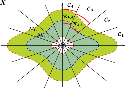
Figure 1. IM-based partitioning for a homogeneous CETC system. The rays passing through the origin determine the cones $\mathcal{C}_{j}$. The dashed lines are consecutive approximations of IMs $M_{t_{k}}$ and $M_{t_{k+1}}$. The regions $\mathcal{R}_{k,j}$ are delimited by consecutive approximations of IMs and cones (hence the indexing). The circular segments in cones $\mathcal{C}_{3}$ and $\mathcal{C}_{4}$ delimit the ball segments that overapproximate regions $\mathcal{R}_{k,3}$ and $\mathcal{R}_{k,4}$.

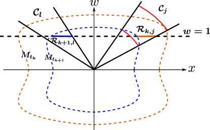
Figure 2. IM-based partitioning for a non-homogeneous CETC system, which has been embedded in ${}^{n_{\zeta}+1}$. The mapped state-space $\tilde{X}$ is a subset of the $w=1$-plane. The rays passing through the origin determine the polyhedral cones $\mathcal{C}_{j}$. The dashed curves are consecutive approximations of IMs $M_{t_{k}}$ and $M_{t_{k+1}}$. The regions $\mathcal{R}_{k,j}$ are intersections between cones $\mathcal{C}_{j}$, the sets between consecutive approximations of isochronous manifolds $M_{t_{k}}$ and $M_{t_{k+1}}$ and the set $\tilde{X}$ (hence the indexing). The circular segments in cone $\mathcal{C}_{j}$ delimit the ball segment, say $\mathcal{B}_{k,j}$, which defines an overapproximation of $\mathcal{R}_{k,j}$ as follows: $\mathcal{R}_{k,j}\subseteq\mathcal{B}_{k,j}\cap\tilde{X}$.

Generally, grid-partitioning is more computationally efficient w.r.t. the computational load of creating the abstraction. On the other hand, IM-based partitioning generally provides tighter intervals $[\underline{\tau}_{\mathcal{R}_{i}},\overline{\tau}_{\mathcal{R}_{i}}]$, thus reducing one of the abstraction’s sources of non-determinism. However, the current implementation of the tool does not check if the given manifolds_times result into approximations of isochronous manifolds which cover the whole state-space of interest $X$; thus, in IM-based partitioning, the user has to inspect the end-result to verify that the state-space is indeed covered by the regions $\mathcal{R}_{i}$. Finally, we note that even when grid-partitioning is employed, the tool uses approximations of isochronous manifolds to derive estimates on timing lower bounds $\underline{\tau}_{\mathcal{R}_{i}}$ and use them as a starting-point for the line-search algorithms, thus speeding up computations. For more information on the abstractions’ construction and on approximations of isochronous manifolds the reader is referred to (Delimpaltadakis and Mazo Jr., 2020, 2021a) and (Delimpaltadakis and Mazo Jr., 2021b, c), respectively.

3.2. Traffic abstractions of linear PETC systems

In the case of unperturbed linear systems under PETC, the construction of abstractions can be performed with simpler computations, provide exact simulations (thanks to the periodic nature of condition checking), and in general the abstractions are tighter than when employing the general scheme described in the previous section.

Consider the PETC system (1),(4) where the plant is a linear system without disturbances

$$\dot{\boldsymbol{\zeta}}(t)=\boldsymbol{A}\boldsymbol{\zeta}(t)+\boldsymbol{B}\boldsymbol{K}\boldsymbol{\zeta}(t_{i})),\quad t\in[t_{i},t_{i+1}),$$

where $\boldsymbol{A}$ and $\boldsymbol{B}$ are the plant matrices and $\boldsymbol{K}$ is the controller gain. Suppose further that the triggering function is quadratic, i.e., $\phi(\boldsymbol{\zeta}(t),\boldsymbol{\zeta}(t_{i}))=\begin{bmatrix}\boldsymbol{\zeta}(t)\\ \boldsymbol{\zeta}(t_{i})\end{bmatrix}^{\mkern-1.5mu\mathsf{T}}\!\!\boldsymbol{Q}\begin{bmatrix}\boldsymbol{\zeta}(t)\\ \boldsymbol{\zeta}(t_{i})\end{bmatrix}.$ Such quadratic triggering functions include the most common ones in the literature (Heemels et al., 2013). This case has some special properties that allow for tighter abstractions than in the nonlinear case. First, from any sampled state one can determine exactly the state reached after $k$:

(7) $$\boldsymbol{\zeta}(t) =\boldsymbol{M}(kh)\boldsymbol{\zeta}_{\boldsymbol{x}}(t_{i}),\ \forall t\in[t_{i},t_{i+1}]$$

$$\boldsymbol{M}(t) \coloneqq\mathrm{e}^{\boldsymbol{A}t}+\int_{0}^{t}\mathrm{e}^{\boldsymbol{A}\tau}\mathrm{d}\tau\boldsymbol{B}\boldsymbol{K}\eqqcolon\boldsymbol{A}_{\mathrm{d}}(t)+\boldsymbol{B}_{\mathrm{d}}(t)\boldsymbol{K}.$$

An isochronous subset, which is the part of the state space that triggers at a given inter-sample time $k$, can be implicitly represented by a conjunction of quadratic inequalities (de A. Gleizer and Mazo Jr., 2020):

(8) $$\begin{gathered}\mathcal{R}_{k}\coloneqq\mathcal{Q}_{k}\setminus\left(\bigcap_{j=1}^{k-1}\mathcal{Q}_{j}\right)=\mathcal{Q}_{k}\cap\bigcap_{j=1}^{k-1}\bar{\mathcal{Q}}_{j},\\ \mathcal{Q}_{k}\coloneqq\begin{cases}\{\boldsymbol{x}\in\mathbb{R}^{n_{\zeta}}\mid\boldsymbol{x}^{\mkern-1.5mu\mathsf{T}}\!\boldsymbol{N}(hk)\boldsymbol{x}>0\},&k<k_{\max{}},\\ \mathbb{R}^{n_{\zeta}},&k=k_{\max{}},\end{cases},\\ \boldsymbol{N}(hk)\coloneqq\begin{bmatrix}\boldsymbol{M}(hk)\\ {\textbf{I}}\end{bmatrix}^{\mkern-1.5mu\mathsf{T}}\!\boldsymbol{Q}\begin{bmatrix}\boldsymbol{M}(hk)\\ {\textbf{I}}\end{bmatrix}.\end{gathered}$$

In (8), the set $\mathcal{Q}_{k}$ is the set of all points in the state-space that certainly triggered by time $hk$; then the set $\mathcal{R}_{k}$ is the isochronous subset obtained by removing from $\mathcal{Q}_{k}$ all points that have triggered before, i.e., $\mathcal{Q}_{j},j<k$. The sets $\mathcal{R}_{k}$ can be checked for non-emptiness exactly via nonlinear satisfiability-modulo-theories (SMT) solvers, e.g., Z3 (De Moura and Bjørner, 2008), or approximately through a semi-definite relaxation (SDR) as proposed in (de A. Gleizer and Mazo Jr., 2020). The non-empty sets form the finite state-space of a quotient system (Tabuada, 2007), which gives formally a (exact) simulation relation to the original PETC traffic. Effectively, the sets $\mathcal{R}_{k}$ form a partition of $\mathbb{R}^{n_{\zeta}}$, and each $\mathcal{R}_{k}$ is a conjunction of finitely many quadratic cones, as depicted in Fig. 3.

Figure 3. An example of isochronous subsets $\mathcal{R}_{k}$ for a two-dimensional linear PETC system.

The transition relation is as well a problem of checking non-emptiness of an intersection of quadratic inequalities:

(9) $$\exists\boldsymbol{x}\in\mathcal{R}_{i}:\boldsymbol{M}(hk)\boldsymbol{x}\in\mathcal{R}_{j}\implies\mathcal{R}_{i}\xrightarrow{k}\mathcal{R}_{j}.$$

Similar to the CETC case, the state space of the abstraction is composed of the regions $\mathcal{R}_{k}$; however, the output set is now finite, $\mathcal{Y}=\{1,2,...,k_{\max}\}$. The transition set is composed of all triplets $\mathcal{R}_{i}\xrightarrow{k}\mathcal{R}_{j}$ satisfying (9); for scheduler synthesis (see Sec. 3.3), the action set is $\mathcal{U}=\mathcal{Y}$, meaning that the scheduler chooses the inter-sample time $kh$, often limited to be smaller than the PETC’s inter-sample time $ih$. For verification, we drop the action set and the transitions are $\mathcal{R}_{i}\xrightarrow{}\mathcal{R}_{j}\coloneqq\mathcal{R}_{i}\xrightarrow{i}\mathcal{R}_{j}$. In both cases, we have effectively a finite transition system (see an example in Fig. 4), in contrast to the CETC case where the inter-sample time can still be chosen on a real interval.

Figure 4. A simple PETC traffic model with only two regions and $k_{\max}=3.$.

Note that using relaxations for an existence problem such as the one above can lead to spurious transitions. From an abstraction (and simulation) perspective, this is acceptable, as it only adds nondeterminism to the abstraction; any scheduler that works for such an abstraction will work for the original system. Nevertheless, the more one can remove spurious non-determinism, the better, thus using exact solvers such as Z3 is recommended if the dimensions of the system permit. Further tightening can be obtained by using the refinements described in (de A. Gleizer and Mazo Jr., 2021b), where isochronous subsets were extended to isosequential subsets, that is, sets $\mathcal{R}_{k_{1}k_{2}k_{3}...k_{l}}$ containing the states whose next $l$ inter-sample times are $hk_{1},hk_{2},...hk_{l}$. This effectivelly chooses the depth of the abstraction refinement one wants to use for the traffic model. In ETCetera, the user can set the depth value and choose solver in {’sdr’, ’z3’}; see §4.5 for an example.

3.3. Scheduler synthesis

Once one has constructed traffic models, they can be employed for the synthesis of schedulers. The goal of a scheduler, in our context, is to specify when each of the considered ETC systems should trigger, such that no overlap of their events occur, while still retaining stability of each of the ETC systems (which is guaranteed if always triggering before $\tau(x)$).

The tool currently considers two methods to synthesize schedulers. The first method relies on the use of UPPAAL. As already indicated in Section 3.1, the general traffic models constructed by ETCetera are equivalent to Timed Automata. Our tool exports the resulting models as timed automata that can be read and manipulated by UPPAAL to synthesize schedulers or check properties of the systems at hand.

The second synthesis method (van Straalen, 2021) follows from recognizing that the specialized traffic models constructed for PETC are finite transition systems (see Sec. 3.2). As such this method is only applicable for these traffic models. Furthermore it is assumed that the sampling time for each of the systems is identical. First, the representation of the traffic models is modified such that it acts on a per-sample basis. Instead of having actions corresponding to the next inter-sample time $\mathcal{U}=\mathcal{Y}=\{1,2,\ldots,k_{max}\}$ as in the models described in Section 3.2, a system can either wait (‘$w$’) , or trigger (‘$t$’) at the current sampling time. The result is a new transition system $\hat{\mathcal{S}}=(\hat{\mathcal{X}},\hat{\mathcal{X}}_{0},\hat{\mathcal{U}},\hat{\mathcal{E}},\hat{\mathcal{Y}},\hat{H})$, where:

• $\hat{\mathcal{X}}:=\{T_{x}\mid x\in\mathcal{X}\}\cup\{W_{x,j}\mid j<H(x),\,x\in\mathcal{X}\}$,

• $\hat{\mathcal{X}}_{0}\subseteq\{T_{x}\mid x\in\mathcal{X}\}$,

• $\hat{\mathcal{U}}:=\{w,t\}$,

• $\hat{\mathcal{E}}:=\{(T_{x},t,T_{x^{\prime}})\mid(x,1,x^{\prime})\in\mathcal{E}\}\allowbreak\cup\{(W_{x,j},w,W_{x,j+1})\mid 1\leq j<H(x)-1\}\allowbreak\cup\{(W_{x,j},t,T_{x^{\prime}})\mid(x,j+1,x^{\prime})\in\mathcal{E}\}$,

• $\hat{\mathcal{Y}}=\{T_{1},T,1,\dots,k_{max}-1\}$,

• $\hat{H}(T_{x})=T_{1}$ if $H(x)=1$, or $T$ otherwise, and $\hat{H}(W_{i,j})=H(i)-j$.

The outputs indicate either whether the system has just triggered (outputs $T_{1}$ and $T$)) or the triggering deadline. Some states are given, for technical reasons, the distinct output $T_{1}$ to capture that from those states the only action that can be taken is ‘$t$’, while on the other states with output $T_{i}\,(i>1)$, both ‘$w$’ and ‘$t$’ actions are enabled. In this transition system, triggering after $k$ samples becomes a sequence of $k-1$ ‘$w$’ actions followed by a single ‘$t$’ action.

Figure 5. An example of wait-trigger model $\hat{\mathcal{S}}$ for PETC traffic.

Next, all these transition systems (representing different PETC systems) are combined into a larger transition system, through a parallel composition allowing each subsystem to behave independently of the rest. Formally, the resulting composition is given by the transition system $\mathcal{S}_{comp.}=(\allowbreak\mathcal{X}_{comp.},\allowbreak\mathcal{X}_{comp.;0},\allowbreak\mathcal{U}_{comp.},\allowbreak\mathcal{E}_{comp.},\allowbreak\mathcal{Y}_{comp.},\allowbreak H_{comp.})$, where

• $\mathcal{X}_{comp.}:=\hat{\mathcal{X}}_{0}\times\dots\times\hat{\mathcal{X}}_{n}$,

• $\mathcal{X}_{comp.;0}:=\hat{\mathcal{X}}_{0;0}\times\dots\times\hat{\mathcal{X}}_{n;0}$,

• $\mathcal{U}_{comp.}:=\hat{\mathcal{U}}_{0}\times\dots\times\hat{\mathcal{U}}_{n}$,

• $\mathcal{E}_{comp.}:=\{((x_{0},\dots,x_{n}),(u_{0},\dots,u_{n}),(x^{\prime}_{0},\dots,x^{\prime}_{n})\allowbreak\mid{\forall i\leq n,}\allowbreak(x_{i},u_{i},x^{\prime}_{i})\in\hat{\mathcal{E}}_{i}\},$

• $\mathcal{Y}_{comp.}:=\hat{\mathcal{Y}}_{0}\times\dots\times\hat{\mathcal{Y}}_{n}$,

• $H_{comp.}(x_{0},\dots,x_{n}):=(\hat{H}_{0}(x_{0}),\dots,\hat{H}_{n}(x_{n}))$.

In this system the behaviour that a scheduler should prevent, i.e. two or more systems triggering simultaneously, is captured by actions which contain two or more more ‘$t$’s. Here it is assumed that the fundamental checking period $h$ of each of the PETC loops is the same. Since after triggering a subsystem always lands in a state with output $T$/$T_{1}$, the scheduler requirement can alternatively be expressed as: ‘Avoid states in $\mathcal{S}_{comp.}$ whose output contains more than one $T$’. Creating a controller that is able to avoid these states can be done effectively for finite transition systems by solving a safety game (c.f. Chapter 6 of (Tabuada, 2009)). In this safety game, the maximal fixed point of the operator

(10) $$F_{W}(Z)=\{x\in Z\,|\,x\in W\land\exists u\in U(x):\>\emptyset\neq Post_{u}(x)\subseteq Z\},$$

is found by iterating over its output (starting with $Z_{0}:=\mathcal{X}_{comp.}$). The set $W$ is the safe set which in this case is given by:

(11) $$W=\{(x_{1},\dots,x_{n})\in\mathcal{X}_{comp.}\,|\,|\{i\mid\hat{H}_{i}(x_{i})\in\{T_{1},T\}\}|\leq 1\}.$$

The maximal fixed point $Z^{*}:=F_{W}(Z^{*})$ contains states in $\mathcal{S}_{comp.}$ (given that $Z^{*}\neq\emptyset$) from which there exists at least one action guaranteeing that a bad state (a collision of triggering events) can be avoided. The scheduler can subsequently be defined as

(12) $$U_{c}(x)=\{u\in\mathcal{U}_{comp.}\mid\emptyset\neq Post_{u}(x)\subseteq Z\}.$$

This is a function that returns a set of safe actions given some state $x\in\mathcal{X}_{comp.}$, which one can obtain from the last sampled states of each of the control systems. The scheduler keeps track of the current state of each $\hat{\mathcal{S}}_{i}$ and based on this collection of states, $U_{c}(x)$ provides a safe action, after which each of the states is updated according to $\hat{\mathcal{E}}_{i}$. Note that after a transmission, due to the non-determinism of the original traffic model, one needs to rely on the value of the measured plant state to determine the corresponding successor state.

To improve the efficiency and scalability of this approach, two additional techniques are implemented (for details see  (van Straalen, 2021)):

1. Partitioning and Refinement: In this approach the size of each $\hat{\mathcal{S}}_{i}$ is reduced by grouping together similar states (partitioning). If no scheduler is found for these reduced systems, these blocks are split apart (refinement) and the safety game is performed again.

2. Binary Decision Diagrams (BDDs) (Bryant, 1992): representing the transition systems with BDDs the manipulation of the transition systems (including partitioning and refinement) can be performed more efficiently, enabling the implementation of the safety-game fixed-point iteration symbolically.

3.4. Other synthesis and analysis problems

As mentioned in the introduction, traffic abstractions for PETC can also be used for quantitative analysis and other synthesis problems, as recently demonstrated in (de A. Gleizer and Mazo Jr., 2021a; de A. Gleizer et al., 2021). For quantitative problems, the transition systems from Def. 1 are equipped with a weight function $\gamma:\mathcal{E}\to\mathbb{Q},$ mapping edges to rational numbers representing the weight or value of a transition. These systems are called weighted transition systems (WTSs) (Chatterjee et al., 2010). For every run $x_{0}\xrightarrow{u_{0}}x_{1}\xrightarrow{u_{1}}x_{2}...$ of $\mathcal{S}$ we can thus compute a sequence of weights $w_{0}w_{1}w_{2}...$, giving rise to the set of all weight sequences $\mathcal{W}_{\mathcal{S}}$. For ETC, we are interested in computing or maximizing the smallest average inter-sample time (SAIST) of a system; hence, the weight of a transition is its inter-sample time. The SAIST of a PETC traffic model $\mathcal{S}$ is formally defined as

(13) $$\mathrm{SAIST}(\mathcal{S})=\inf_{w_{0}w_{1}w_{2}...\in\mathcal{W}_{\mathcal{S}}}\liminf_{n\to\infty}\frac{1}{n+1}\sum_{i=0}^{n}w_{i}.$$

A lower bound to the SAIST of a PETC system can be computed using Karp’s algorithm (Karp, 1978; Chaturvedi and McConnell, 2017) on the abstraction. In some cases, the abstraction can be a smallest-average-cycle-equivalent simulation (de A. Gleizer and Mazo Jr., 2021a; de Albuquerque Gleizer and Jr., 2021), a property that can be verified for PETC of linear systems: in this case, the SAIST from the abstraction is exact.

In order to do synthesis, we equip the PETC traffic model with early-triggering samples as in the scheduling problem, and solve a mean-payoff game (Ehrenfeucht and Mycielski, 1979), obtaining a lower bound to the optimal sampling strategy (de A. Gleizer et al., 2021). The strategy is a function mapping a region $\mathcal{R}_{i}$ onto an inter-sample time choice $k$, becoming effectively a self-triggered control scheme (Velasco et al., 2003; Anta and Tabuada, 2008; Mazo Jr. et al., 2010). The idea behind the approach in (de A. Gleizer et al., 2021) is to sample early in some regions of the state-space to collect long-term benefits, something that the shortsighted ETC cannot do. The abstractions contain long-term traffic information which allows better strategies to be computed. In (de A. Gleizer et al., 2021), the SAIST of a numerical example nearly doubled using this approach.

3.5. Discussion on computational complexity

When abstracting general CETC systems, the size of the state-space partition using either gridding or IMs scales exponentially with $n_{\zeta}$. Nonetheless, in the case of linear PETC, the use of isochronous sets removes the dependence on dimensions, and the number of regions is $\mathcal{O}(k_{max}^{l})$. The complexity of computing IM-approximations mainly depends on the complexity of the dReal (Gao et al., 2013), which is exponential on $n_{\zeta}$ for our problem. Generating timing intervals and transitions, in the case of general CETC systems, is $\mathcal{O}(r)C$ and $\mathcal{O}(r^{2})C$ respectively, where $r$ is the number of regions and $C$ is the complexity of the reachability analysis operation. For linear PETC, the transition relation computation is $O(k_{max}r^{2})C^{\prime}$, where $C^{\prime}$ is polynomial in $n_{\zeta}$ when using solver=’sdr’ (see (de A. Gleizer and Mazo Jr., 2020)) and exponential in $n_{\zeta}$ when using solver=’z3’ (see (de Albuquerque Gleizer and Jr., 2021)). The resulting system $\hat{S}$ for linear PETC has $\mathcal{O}(k_{max}^{l+1})$ states (which is $rk_{max}$) and $\mathcal{O}(k_{max}^{2l+2})$ transitions (which is $rk_{max}^{2}$). In practice, the number of regions often grows much slower than exponentially with $l$, a phenomenon investigated in (Gleizer and Mazo Jr, 2022). Regarding scheduling, using UPPAAL the size of the problem scales exponentially with the number of systems in the network (TA safety games are exponential on the number of clocks). The scheduling technique of Section 3.3 is more efficient, exploiting PETC models being already FTSs. Additionally, partitioning can reduce the number of states to $\mathcal{O}(k_{max})$ (and the transitions accordingly to $\mathcal{O}(k_{max}^{2})$). However, if the safety game fails, refinement has to be performed, increasing the number of states. Introducing BDDs complicates this analysis, see (van Straalen, 2021) for more details. It is important to remark, however, that the abstraction and scheduler synthesis processes are performed offline, with the synthesized scheduler’s online implementation being simply a set of if-then-else rules.

4. Use of ETCetera

ETCetera is implemented in Python, and uses third-party tools cvxpy (Diamond and Boyd, 2016; Agrawal et al., 2018), z3 (De Moura and Bjørner, 2008), dReach (Kong et al., 2015), dReal (Gao et al., 2013) and Flowstar (Chen et al., 2013) for the creation of traffic models, UPPAAL Stratego (David et al., 2015) for scheduler synthesis and dd (Control and Systems, 2020) (with bindings to CUDD  (Somenzi, 1998)) for the manipulation of BDDs. To construct traffic models, the user has two possibilities: (i) employ a command line interface, or (ii) employ the utilities provided inside a python script, as illustrated in detail in the examples in Sections 4.2 and  4.3. Analysis and scheduler synthesis can currently only be performed within a Python script, as shown in the examples of Sections 4.4 and  4.5. The computations of all examples below have been conducted on a laptop with an Intel i7-9750H processor and 16 GB of RAM.

4.1. Command line interface

If the command line interface is employed, the user simply needs to run the following command:

⬇

1$ python etc2traffic.py system_type input_file [options]

This reads the contents of input_file and generates a traffic model. The contents of input_file depend on the system_type (either linear PETC or general). When system_type is linear PETC, input_file looks like:

⬇

1Dynamics : [0 1; -2 3], [0; 1]

2Controller: [1 -4]

3Triggering Sampling Time: 0.01

4Triggering Heartbeat: 0.40

5Triggering Condition: [0.95 0 -1 0;0 0.95 0 -1;-1 0 1 0;0 -1 0 1]

This constructs a specialized PETC traffic model as is described in Section 3.2. Dynamics contains the state evolution matrix ($\boldsymbol{A}$) and the input matrix ($\boldsymbol{B}$), and the Controller contains the feedback gain ($\boldsymbol{K}$). These must all be expressed as matrices. Triggering Sampling Time is the checking period $h$ that is considered and Triggering Heartbeat is the maximum trigger time $(hk_{max})$. Finally, Triggering Condition contains the triggering matrix $\boldsymbol{Q}$ as only quadratic triggering conditions are considered in this case.

When system_type is general, input_file looks like:

⬇

1Hyperbox States : [-2 2], [-2 2]

2Grid Points Per Dimension: [3 3]

3Dynamics : x1, x1^∗∗2^∗x2 + x2^∗∗3 + u1

4Controller: -x2 - x1^∗∗2^∗x2 - x2^∗∗3

5Triggering Condition : e1^∗∗2 + e2^∗∗2 - 0.01^∗∗2

6Solver Options : manifolds_times=[0.002 0.0028 0.0038 0.005 0.0065 0.0075], partition_method=manifold, heartbeat=0.021, order_approx=4

Which constructs a general traffic model as described in Section 3.1. In this case, Dynamics, Controller and Triggering Conditions are specified as symbolic expressions (where $**$ represents exponentiation). State variables are denoted with x1, x2, ..., control variables with u1, u2, ..., error variables with e1, e2, ..., disturbance variables with d1, d2, ... and the variable used for homogenization as w1. Furthermore, the rectangular region of the state space that is to be considered must be supplied in Hyperbox States. Other mandatory arguments depend on: (i) the partition method, (ii) whether the system is homogeneous, (iii) if disturbances are involved:

• If partition_method=grid or when the system is not homogeneous, Grid Points Per Dimension must be specified, which contains the number of regions the state space is divided into for each of the states.

• If partition_method=manifold, then manifolds_times in Solver Options must be specified, which will define the Isochronous Manifolds.

• If disturbances are present, Hyperbox Disturbances must be specified, containing for each disturbance the interval it will lie in.

Other optional parameters can be supplied in Solver Options. In this example heartbeat contains the maximum trigger time and order_approx contains the order of approximation of the isochronous manifolds.

In addition to this command line interface, one can construct traffic models via Python scripts as well, as will be shown in Sections 4.2 and  4.3. The command line interface is currently only available for the construction of traffic models, so for scheduling and analysis purposes the procedures in Sections 4.4 and  4.5 should be followed.

4.2. Python interface: linear PETC abstractions

Consider the linear PETC system:

(14) $$\begin{split}\dot{\zeta}(t)&=\begin{bmatrix}-0.5&0\\ 0&3.5\end{bmatrix}\zeta(t)+\begin{bmatrix}1\\ 1\end{bmatrix}u(\zeta(t_{i})),\\ u(\zeta(t_{i}))&=\begin{bmatrix}1.02&-5.62\end{bmatrix}\zeta(t_{i}),\end{split}\quad t\in[t_{i},t_{i+1})$$

with triggering function $\phi(\zeta(t),\zeta(t_{i}))=|\zeta(t)-\zeta(t_{i})|^{2}-(1-\sigma)\left|\zeta(t)\right|^{2}$, where $\sigma=0.05$ and $h=0.01$, $k_{max}=20$. The PETC traffic model for this system is generated as follows:

⬇

1import numpy as np

2

3# Define LTI system matrices

4A = np.array([[-0.5, 0], [0, 3.5]])

5B = np.array([[1],[1]])

6K = np.array([[1.02, -5.62]])

7

8# PETC parameters

9h = 0.01

10kmax = 20

11sigma = 0.05

12

13# Triggering condition

14Qtrigger = np.block([[(1-sigma)^∗np.eye(2), -np.eye(2)], [-np.eye(2), np.eye(2)]])

15

16# Construct object representing the PETC system

17import ETCetera.Systems as systems

18

19plant = systems.LinearPlant(A, B)

20controller = systems.LinearController(K, h)

21trigger = systems.LinearQuadraticPETC(plant, controller, kmax=kmax, Qbar=Qtrigger)

22

23# Create Traffic Model

24import ETCetera.Abstractions as abstr

25

26traffic = abstr.TrafficModelLinearPETC(trigger)

27regions, transitions = traffic.create_abstraction()

4.3. Python interface: nonlinear CETC abstractions

Consider the nonlinear CETC system:

(15) $$\begin{split}\dot{\zeta}(t)&=\begin{bmatrix}\zeta_{1}(t)\\ \zeta_{1}^{2}(t)\zeta_{2}(t)+\zeta_{2}^{3}(t)+u(\zeta(t_{i}))\end{bmatrix},\\ u(\zeta(t_{i}))&=-\zeta_{2}(t_{i})-\zeta_{1}^{2}(t)\zeta_{2}(t)-\zeta_{2}^{3}(t),\end{split}\quad t\in[t_{i},t_{i+1})$$

together with the triggering condition $\phi(\zeta(t),\zeta(t_{i}))=|\zeta(t)-\zeta(t_{i})|^{2}-0.01^{2}$. The CETC system may be defined as follows:

⬇

1import sympy

2

3# Define

4state_vector = x1, x2, e1, e2 \

5 = sympy.symbols(’x1 x2 e1 e2’)

6

7# Define controller (in etc form)

8u1 = -(x2+e2) - (x1+e1)^∗∗2^∗(x2+e2) - (x2+e2)^∗∗3

9

10# Define dynamics

11x1dot = -x1

12x2dot = x1^∗∗2^∗x2 + x2^∗∗3 + u1

13dynamics = [x1dot, x2dot, -x1dot, -x2dot]

14

15# Triggering condition & other etc.

16trigger = e1 ^∗∗ 2 + e2 ^∗∗ 2 - 0.01^∗∗2

17

18# State space limits

19state_space_limits = [[-2, 2], [-2, 2]]

20grid_points_per_dim = [3,3]

A traffic model for this system is then simply constructed with:

⬇

1import ETCetera.Abstractions as abstr

2

3# Partition method manifold

4traffic = abstr.TrafficModelNonlinearETC(dynamics, trigger, state_vector, state_space_limits=state_space_limits, grid_points_per_dim=grid_points_per_dim, manifolds_times=[0.002, 0.0028, 0.0038, 0.005, 0.0065, 0.0075], partition_method=’manifold’, heartbeat=0.021, order_approx=4)

5regions, transitions = traffic.create_abstraction()

Plots of lower and upper bounds on the inter-sample times and transitions for the resulting traffic model can be generated by running the command traffic.visualize(), and they are shown in Figure 6. The total CPU time was about 1 hour.

To add disturbances to the dynamics, the corresponding parameters (d1,...) and their domain dist_param_domain have to be declared, as well as partition_method=’grid’ has to be specified:

⬇

1d1 = sympy.symbols(’d1’)

2x1dot = -x1

3x2dot = x1^∗∗2^∗x2 + x2^∗∗3 + u1 + d1

4dynamics = [x1dot, x2dot, -x1dot, -x2dot]

5disturbace_limits = [[-0.1, 0.1]]

6traffic = abstr.TrafficModelNonlinearETC(dynamics, trigger, state_vector, state_space_limits=state_space_limits, dist_param=(d1,), dist_param_domain=disturbace_limits, order_approx=2, heartbeat=0.022, grid_points_per_dim=[7,8], partition_method=’grid’, precision_deltas=1e-6)

(a) Lower and upper bounds of the inter-sample times for each of the regions of the traffic model generated in Example 4.3

(b) Transition between the regions of the traffic model generated in Example 4.3

Figure 6. Example 4.3 results.

4.4. Scheduler synthesis

In this example, the complete workflow of generating a scheduler for two linear PETC systems is described. Consider the two systems (Tabuada, 2007; Hetel et al., 2011):

(16) $$\begin{split}\dot{\zeta}_{1}(t)&=\begin{bmatrix}0&1\\ -2&3\end{bmatrix}\zeta_{1}(t)+\begin{bmatrix}0\\ 1\end{bmatrix}u_{1}(\zeta_{1}(t_{i})),\\ u_{1}(\zeta_{1}(t_{i}))&=\begin{bmatrix}1&-4\end{bmatrix}\zeta_{1}(t_{i}),\\ \dot{\zeta}_{2}(t)&=\begin{bmatrix}-0.5&0\\ 0&3.5\end{bmatrix}\zeta_{2}(t)+\begin{bmatrix}1\\ 1\end{bmatrix}u_{2}(\zeta_{2}(t_{i})),\\ u_{2}(\zeta_{2}(t_{i}))&=\begin{bmatrix}1.02&-5.62\end{bmatrix}\zeta_{2}(t_{i}),\end{split}\quad t\in[t_{i},t_{i+1})$$

both with triggering condition $\phi(\zeta(t),\zeta(t_{i}))=|\zeta(t)-\zeta(t_{i})|^{2}-(1-\sigma)\left|\zeta(t)\right|^{2}$, where $\sigma=0.05$ and $h=0.01$, $k_{1,max}=40$, $k_{2,max}=20$. These two systems have been defined in files as specified in Section 4.1. A scheduler can then be synthesized and simulated as follows:

⬇

1from ETCetera.util import ^∗

2

3# First construct the traffic models

4traffic1 = construct_linearPETC_traffic_from_file(’examples/linear_2.txt’)

5traffic2 = construct_linearPETC_traffic_from_file(’examples/linear_3.txt’)

6

7import ETCetera.Scheduling.fpiter as sched

8

9# Convert traffic models into different form

10cl1 = sched.controlloop(traffic1)

11cl2 = sched.controlloop(traffic2)

12

13# Construct system and generate scheduler

14S = sched.system([cl1, cl2])

15Ux, _ = S.generate_safety_scheduler()

16

17# Simulate

18S.simulate(x0=[[1,1],[1,-1]], Tmax=5)

The results of the simulation are shown in Figures 7 and  8. The total CPU time was 10 minutes. By default, this synthesis approach makes use of BDDs. To make this process more insightful, one can specify use_bdd=False in the construction of the control loop. However, this can drastically impact performance of the synthesis process.

Creating schedulers using UPPAAL follows the same steps, with the exception that additionally a network has to be defined:

⬇

1import ETCetera.Scheduling.NTGA as sched

2

3cl1 = sched.controlloop(traffic1)

4cl2 = sched.controlloop(traffic2)

5

6# Define a network and combine

7net = sched.network()

8nta = sched.nta(net, [cl1, cl2])

9

10# Generate a strategy using UPPAAL and parse its results

11nta.generate_strategy(parse_strategy=True)

(a) State evolution of system 1 with initial condition $x_{0}={[1,1]}^{T}$.

(b) State evolution of system 2 with initial condition $x_{0}={[1,-1]}^{T}$.

Figure 7. Evolution of the systems’ states under the scheduler synthesized as detailed in Section 4.4. Dashed lines represent the actual state evolution, while the solid lines represent the states available to the controller at each time.

(a) Sampling times with the use of the synthesized scheduler.

(b) Sampling times without the use of a scheduler.

Figure 8. Sampling times of the first 1.2 seconds of the simulation in Figure 7. For reference, the sampling times when no scheduler is used are shown in (b). Early triggers are denoted with a ‘$\circ$’. Sampling collisions are represented with a ‘$\Diamond$’.

4.5. Quantitative analysis and synthesis

Consider the first system in (16). In this example we are interested in obtaining a large average inter-sample time; hence we use the more aggressive Lyapunov-based triggering condition (Szymanek et al., 2019; de A. Gleizer and Mazo Jr., 2021b) of the form $V(\hat{\boldsymbol{\zeta}}(t))>-\rho\hat{\boldsymbol{\zeta}}(t)^{\mkern-1.5mu\mathsf{T}}\!\boldsymbol{Q}_{\mathrm{Lyap}}\hat{\boldsymbol{\zeta}}(t),$ where $\hat{\boldsymbol{\zeta}}(t)\coloneqq\boldsymbol{A}_{\mathrm{d}}(h)\boldsymbol{\zeta}(t)+\boldsymbol{B}_{\mathrm{d}}(h)\boldsymbol{K}\boldsymbol{\zeta}(t_{i})$ is the state prediction after $h$ time units, $V(\boldsymbol{x})=\boldsymbol{x}^{\mkern-1.5mu\mathsf{T}}\!\boldsymbol{P}_{\mathrm{Lyap}}\boldsymbol{x}$, and $0<\rho<1$ is the triggering parameter. For the numerical results below, the Lyapunov matrices were taken from (Tabuada, 2007) as $\boldsymbol{P}_{\mathrm{Lyap}}=\begin{bmatrix}1&0.25\\ 0.25&1\end{bmatrix},\ \boldsymbol{Q}_{\mathrm{Lyap}}=\begin{bmatrix}0.5&0.25\\ 0.25&1.5\end{bmatrix}$, and we set $h=0.1,$ $\rho=0.8$ and $K=20$. The triggering condition used is quadratic and can be specified as in §4.2. The code snippet below (replacing lines 26–27 from the example in §4.2) shows how to

1. construct abstractions to compute the system’s smallest average inter-sample time (SAIST), where we flag etc_only=True to avoid computing unnecessary early-triggering transitions;

2. construct a normal abstraction with early-triggering transitions to synthesize a near-optimal sampling strategy;

3. verify the SAIST of the closed-loop system with the generated strategy.

⬇

26import numpy as np

27

28# Define LTI system matrices

29A = np.array([[0, 1], [-2, 3]])

30B = np.array([[0],[1]])

31K = np.array([[1, -4]])

32

33# PETC parameters

34h = 0.1

35kmax = 20

36

37# Triggering condition

38Qtrigger = np.array([[ -0.14770797, -2.52808495, -0.20224506, 0.80898024], [ -2.52808495, 13.75369717, 2.56242462, -10.24969847], [ -0.20224506, 2.56242462, 0.33917205, -1.3566882 ], [ 0.80898024, -10.24969847, -1.3566882 , 5.42675281]])

39

40# Construct object representing the PETC system

41import ETCetera.Systems as systems

42

43plant = systems.LinearPlant(A, B)

44controller = systems.LinearController(K, h)

45trigger = systems.LinearQuadraticPETC(plant, controller, kmax=kmax, Qbar=Qtrigger)

46

47# Create Traffic Model

48import ETCetera.Abstractions as abstr

49

50

51# Best selection for SAIST: solver=’z3’, etc_only, stop_if_mace_equivalent, smart_mace

52traffic = abstr.TrafficModelLinearPETC(trigger, depth=100, etc_only=True, solver=’z3’, stop_if_mace_equivalent=True, smart_mace=True)

53regions, transitions = traffic.create_abstraction()

54

55# Print obtained SAIST and its minimizing cycle

56print(f’SAIST is {traffic.limavg}’); print(f’Smallest average cycles: {traffic.cycles}’)

57

58# Now create an abstraction to design an improved sampling strategy

59traffic_synth = abstr.TrafficModelLinearPETC(trigger, depth=1, etc_only=False, solver=’z3’, early_trigger_only=True)

60strat, strat_tran = traffic_synth.optimize_sampling_strategy()

61print(strat) # Inspect strategy

62

63# Compute its SAIST value

64traffic2 = abstr.TrafficModelLinearPETC(trigger, depth=100, etc_only=True, solver=’z3’, stop_if_mace_equivalent=True, smart_mace=True, strategy=strat, strategy_transition=strat_tran)

65regions2, transitions2 = traffic2.create_abstraction()

66print(f’Optimized SAIST is {traffic2.limavg}’)

This code reproduces part of the results in (de A. Gleizer et al., 2021), giving the following output (the numbers are normalized by $h$):

⬇

1SAIST is 2.3333333333333335

2Smallest average cycles: {(8, 1, 1, 1, 1, 2)}

3Optimized SAIST is 5.0

The algorithm terminated in 5 minutes.

5. Conclusions and future work

We have introduced the tool ETCetera enabling the study and manipulation of the inter-sample times generated by event-triggered control systems. The main functionality of the tool is to create abstract traffic models from the inter-sample times dynamics implicitly determined by the hybrid dynamics of ETC systems. The tool allows to construct traffic models in the form of timed-automata for general ETC systems, and in the form of finite transition systems in the particular case of PETC systems. The resulting models can be exported for further analysis to UPPAAL, in the case of timed-automata models, or manipulated within the tool (in the case of PETC systems). ETCetera provides algorithmic implementations to synthesize schedulers, compute performance metrics, and design improved sampling strategies for traffic models of PETC systems. The tool is available as an open-source project and continuously being extended with additional functionalities. In particular ongoing and future work is focusing on the following:

• IM-based partitioning for systems with disturbances. Even though the theory developed in (Delimpaltadakis and Mazo Jr., 2021a) addresses this case, this is not yet implemented as Flow* cannot handle ball-segments and dReach cannot handle disturbances.

• In (Delimpaltadakis and Mazo Jr., 2021a) it has been observed that IM-based partitioning, sometimes, results into more transitions, probably because the sets $\mathcal{R}_{i}$ are approximated by ball-segments (which may be a crude approximation). We are working on tackling this issue (with tighter approximations) in future versions of the tool.

• Based on the developments of (Delimpaltadakis et al., 2021) and (Delimpaltadakis et al., 2022), extend abstractions to stochastic PETC systems via interval markov decision processes, for verification of various performance metrics and for scheduler synthesis with probabilistic safety.

• Automate the synthesis of schedulers for PETC loops not sharing the same fundamental sampling time $h$.

• Extend the specialized models of linear PETC traffic to perturbed systems, output-feedback systems and CETC.

• Enable the simulation of multiple ETC loops under a synthesized scheduler over the network simulator OMNET++ (Varga, 2010).

- (1)
- Åarzén (1999) Karl-Erik Åarzén. 1999. A simple event-based PID controller. IFAC Proceedings Volumes 32, 2 (1999), 8687–8692.
- Agrawal et al. (2018) Akshay Agrawal, Robin Verschueren, Steven Diamond, and Stephen Boyd. 2018. A rewriting system for convex optimization problems. Journal of Control and Decision 5, 1 (2018), 42–60.
- Alur and Dill (1994) Rajeev Alur and David L Dill. 1994. A theory of timed automata. Theoretical computer science 126, 2 (1994), 183–235.
- Anta and Tabuada (2008) Adolfo Anta and Paulo Tabuada. 2008. Self-triggered stabilization of homogeneous control systems. In American Control Conference, 2008. IEEE, 4129–4134.
- Astrom and Bernhardsson (2002) Karl Johan Astrom and Bo M Bernhardsson. 2002. Comparison of Riemann and Lebesgue sampling for first order stochastic systems. In Proceedings of the 41st IEEE Conference on Decision and Control, 2002., Vol. 2. IEEE, 2011–2016.
- Bryant (1992) Randal E Bryant. 1992. Symbolic boolean manipulation with ordered binary-decision diagrams. ACM Computing Surveys (CSUR) 24, 3 (1992), 293–318.
- Chatterjee et al. (2010) Krishnendu Chatterjee, Laurent Doyen, and Thomas A Henzinger. 2010. Quantitative languages. ACM Transactions on Computational Logic (TOCL) 11, 4 (2010), 1–38.
- Chaturvedi and McConnell (2017) Mmanu Chaturvedi and Ross M McConnell. 2017. A note on finding minimum mean cycle. Inform. Process. Lett. 127 (2017), 21–22.
- Chen et al. (2013) Xin Chen, Erika Ábrahám, and Sriram Sankaranarayanan. 2013. Flow*: An analyzer for non-linear hybrid systems. In International Conference on Computer Aided Verification. Springer, 258–263.
- Control and Systems (2020) Caltech Control and Dynamical Systems. 2020. dd (version 0.5.6.). https://pypi.org/project/dd/.
- David et al. (2015) Alexandre David, Peter Gjøl Jensen, Kim Guldstrand Larsen, Marius Mikučionis, and Jakob Haahr Taankvist. 2015. Uppaal stratego. In International Conference on Tools and Algorithms for the Construction and Analysis of Systems. Springer, 206–211.
- de A. Gleizer et al. (2021) Gabriel de A. Gleizer, Khushraj Madnani, and Manuel Mazo Jr. 2021. Self-Triggered Control for Near-Maximal Average Inter-Sample Time. In 60th IEEE Conference on Decision and Control (accepted).
- de A. Gleizer and Mazo Jr. (2020) Gabriel de A. Gleizer and Manuel Mazo Jr. 2020. Scalable traffic models for scheduling of linear periodic event-triggered controllers. IFAC-PapersOnLine 53, 2 (2020), 2726–2732.
- de A. Gleizer and Mazo Jr. (2021a) Gabriel de A. Gleizer and M. Mazo Jr. 2021a. Computing the sampling performance of event-triggered control. In Proc. of the 24th Int’l Conf. on Hybrid Systems: Computation and Control (Nashville, TN, USA) (HSCC ’21). ACM, Article 20, 7 pages.
- de A. Gleizer and Mazo Jr. (2021b) Gabriel de A. Gleizer and Manuel Mazo Jr. 2021b. Towards Traffic Bisimulation of Linear Periodic Event-Triggered Controllers. IEEE Control Systems Letters 5, 1 (2021), 25–30.
- de Albuquerque Gleizer and Jr. (2021) Gabriel de Albuquerque Gleizer and Manuel Mazo Jr. 2021. Computing the average inter-sample time of event-triggered control using quantitative automata. arXiv:2109.14391 [eess.SY]
- De Moura and Bjørner (2008) Leonardo De Moura and Nikolaj Bjørner. 2008. Z3: An efficient SMT solver. In International conference on Tools and Algorithms for the Construction and Analysis of Systems. Springer, 337–340.
- Delimpaltadakis et al. (2021) Giannis Delimpaltadakis, Luca Laurenti, and Manuel Mazo Jr. 2021. Abstracting the Sampling Behaviour of Stochastic Linear Periodic Event-Triggered Control Systems. In 2021 60th IEEE Conference on Decision and Control (CDC). 1287–1294. https://doi.org/10.1109/CDC45484.2021.9683751
- Delimpaltadakis et al. (2022) Giannis Delimpaltadakis, Luca Laurenti, and Manuel Mazo Jr. 2022. Formal Analysis of the Sampling Behaviour of Stochastic Event-Triggered Control. arXiv preprint arXiv:2202.10178 (2022).
- Delimpaltadakis and Mazo Jr. (2020) Giannis Delimpaltadakis and Manuel Mazo Jr. 2020. Traffic Abstractions of Nonlinear Homogeneous Event-Triggered Control Systems. In 2020 59th IEEE Conference on Decision and Control (CDC). 4991–4998. https://doi.org/10.1109/CDC42340.2020.9303968
- Delimpaltadakis and Mazo Jr. (2021a) Giannis Delimpaltadakis and Manuel Mazo Jr. 2021a. Abstracting the Traffic of Nonlinear Event-Triggered Control Systems. arXiv preprint arXiv:2010.12341, under review (2021).
- Delimpaltadakis and Mazo Jr. (2021b) Giannis Delimpaltadakis and Manuel Mazo Jr. 2021b. Isochronous Partitions for Region-Based Self-Triggered Control. IEEE Trans. Automat. Control 66, 3 (2021), 1160–1173. https://doi.org/10.1109/TAC.2020.2994020
- Delimpaltadakis and Mazo Jr. (2021c) Giannis Delimpaltadakis and Manuel Mazo Jr. 2021c. Region-Based Self-Triggered Control for Perturbed and Uncertain Nonlinear Systems. IEEE Transactions on Control of Network Systems 8, 2 (2021), 757–768. https://doi.org/10.1109/TCNS.2021.3050121
- Diamond and Boyd (2016) Steven Diamond and Stephen Boyd. 2016. CVXPY: A Python-embedded modeling language for convex optimization. Journal of Machine Learning Research 17, 83 (2016), 1–5.
- Ehrenfeucht and Mycielski (1979) Andrzej Ehrenfeucht and Jan Mycielski. 1979. Positional strategies for mean payoff games. International Journal of Game Theory 8, 2 (1979), 109–113.
- Fiter et al. (2012) Christophe Fiter, Laurentiu Hetel, Wilfrid Perruquetti, and Jean-Pierre Richard. 2012. A state dependent sampling for linear state feedback. Automatica 48, 8 (2012), 1860–1867.
- Gao et al. (2013) Sicun Gao, Soonho Kong, and Edmund M Clarke. 2013. dReal: An SMT solver for nonlinear theories over the reals. In International Conference on Automated Deduction. Springer, 208–214.
- Gleizer and Mazo Jr (2022) Gabriel de Albuquerque Gleizer and Manuel Mazo Jr. 2022. Chaos and order in event-triggered control. arXiv preprint arXiv:2201.04462 (2022).
- Heemels et al. (2013) W. P. M. H. Heemels, M. C. F. Donkers, and Andrew R. Teel. 2013. Periodic event-triggered control for linear systems. IEEE Trans. Automat. Control 58, 4 (2013), 847–861.
- Hetel et al. (2011) L. Hetel, A. Kruszewski, W. Perruquetti, and J. Richard. 2011. Discrete and Intersample Analysis of Systems With Aperiodic Sampling. IEEE Trans. Automat. Control 56, 7 (2011), 1696–1701. https://doi.org/10.1109/TAC.2011.2122690
- Karp (1978) Richard M Karp. 1978. A characterization of the minimum cycle mean in a digraph. Discrete mathematics 23, 3 (1978), 309–311.
- Kolarijani and Mazo Jr (2016) Arman Sharifi Kolarijani and Manuel Mazo Jr. 2016. Formal Traffic Characterization of LTI Event-Triggered Control Systems. IEEE Transactions on Control of Network Systems 5, 1 (2016), 274–283.
- Kong et al. (2015) Soonho Kong, Sicun Gao, Wei Chen, and Edmund Clarke. 2015. dReach: -reachability analysis for hybrid systems. In International Conference on TOOLS and Algorithms for the Construction and Analysis of Systems. Springer, 200–205.
- Mazo Jr. et al. (2010) Manuel Mazo Jr., Adolfo Anta, and Paulo Tabuada. 2010. An ISS self-triggered implementation of linear controllers. Automatica 46, 8 (2010), 1310–1314.
- Mazo Jr et al. (2018) Manuel Mazo Jr, Arman Sharifi-Kolarijani, Dieky Adzkiya, and Christiaan Hop. 2018. Abstracted models for scheduling of event-triggered control data traffic. In Control Subject to Computational and Communication Constraints. Springer, 197–217.
- Postoyan et al. (2019) R. Postoyan, R. G. Sanfelice, and W. P. M. H. Heemels. 2019. Inter-event Times Analysis for Planar Linear Event-triggered Controlled Systems. In 2019 IEEE 58th Conference on Decision and Control (CDC). 1662–1667. https://doi.org/10.1109/CDC40024.2019.9028888
- Rajan and Tallapragada (2020) A. Rajan and P. Tallapragada. 2020. Analysis of Inter-Event Times for Planar Linear Systems Under a General Class of Event Triggering Rules. In 2020 59th IEEE Conference on Decision and Control (CDC). 5206–5211. https://doi.org/10.1109/CDC42340.2020.9304406
- Somenzi (1998) F. Somenzi. 1998. CUDD: CU Decision Diagram Package Release 2.2.0.
- Szymanek et al. (2019) Aleksandra Szymanek, Gabriel de A. Gleizer, and Manuel Mazo Jr. 2019. Periodic event-triggered control with a relaxed triggering condition. In 2019 IEEE 58th Conference on Decision and Control (CDC). IEEE, 1656–1661.
- Tabuada (2007) Paulo Tabuada. 2007. Event-triggered real-time scheduling of stabilizing control tasks. IEEE Trans. Automat. Control 52, 9 (2007), 1680–1685.
- Tabuada (2009) Paulo Tabuada. 2009. Verification and control of hybrid systems: a symbolic approach. Springer Science & Business Media.
- van Straalen (2021) Ivo van Straalen. 2021. Efficient Scheduler Synthesis For Periodic Event Triggered Control Systems: An Approach With Binary Decision Diagrams. Master’s thesis. Delft University of Technology. http://resolver.tudelft.nl/uuid:f9764019-e908-45e7-a053-0f6fbc8a7792
- Varga (2010) Andras Varga. 2010. OMNeT++. In Modeling and tools for network simulation. Springer, 35–59.
- Velasco et al. (2003) Manel Velasco, Josep Fuertes, and Pau Marti. 2003. The self triggered task model for real-time control systems. In Work-in-Progress Session of the 24th IEEE Real-Time Systems Symposium (RTSS03), Vol. 384.