Absence of confinement and non-Boltzmann stationary states of fractional Brownian motion in shallow external potentials

Abstract

We study the diffusive motion of a particle in a subharmonic potential of the form $U(x)=|x|^{c}$ ($0<c<2$) driven by long-range correlated, stationary fractional Gaussian noise $\xi_{\alpha}(t)$ with $0<\alpha\leq 2$. In the absence of the potential the particle exhibits free fractional Brownian motion with anomalous diffusion exponent $\alpha$. While for an harmonic external potential the dynamics converges to a Gaussian stationary state, from extensive numerical analysis we here demonstrate that stationary states for shallower than harmonic potentials exist only as long as the relation $c>2(1-1/\alpha)$ holds. We analyse the motion in terms of the mean squared displacement and (when it exists) the stationary probability density function (PDF). Moreover we discuss analogies of non-stationarity of Lévy flights in shallow external potentials.

1 Introduction

In his seminal PhD thesis published in 1931, Kappler presents the Gaussian equilibrium distribution (Boltzmannian) for the angular co-ordinate of a torsional balance driven by thermal noise [1]. This result is expected from equilibrium statistical physics [2], as long as the angle is sufficiently small and thus the restoring effect on the angular motion, exerted by the suspending glass thread, can be approximated by a Hookean force. On microscopic scales such an harmonic confinement and the associated equilibrium fluctuations for a diffusing particle in water can be effected by a polymeric tether [3, 4].

Harmonic confinement of micron-sized dielectric tracer particles in simple liquids is now routinely achieved by optical tweezers [5]. The equilibration from a non-equilibrium initial condition of the tracer can be derived from the associated Fokker-Planck-Smoluchowski or Langevin equations and turns out to be exponentially fast [6, 7, 8]. In more complex fluids such as viscoelastic liquids the relaxation to an equilibrium situation of a tracer confined by an optical tweezers trap still occurs albeit with more complex dynamics including transient non-ergodicity [9, 10, 11]. For ageing, weakly non-ergodic dynamics the approach to the Boltzmannian state may be much slower [12, 13] and, when time-averaged observables are evaluated, obscured by a crossover to a power-law instead of a plateau [14, 15], as shown in optical tweezers measurements of tracer particles [16] and for the relative motion of subunits of single protein molecules [18, 17].

What happens when the external potential deviates from the conventional harmonic shape? Steeper than harmonic potentials occur, for instance, when the harmonic approximation of the symmetric potential no longer holds and the next order, quartic term needs to be considered. The Boltzmannian in such potentials is flatter around the centre and decays more abruptly at larger distances. For Lévy flights governed by power-law jump length distributions $\simeq|x|^{-1-\mu}$ with $0<\mu<2$ such steeper than harmonic potentials effect non-Boltzmannian, multimodal stationary probability density functions (PDFs) [19, 20, 21, 22]. For fractional Brownian motion driven by power-law correlated, fractional Gaussian noise (FGN, see below for the definition) superharmonic external potentials also lead to non-Boltzmannian PDFs, that in the superdiffusive case may assume multimodal states [23]. Similar effects occur on a finite interval with reflecting boundaries [24]. Shallower than harmonic potentials may emerge as entropic forces, e.g., in specific geometries of confining channels [25, 26], and confining, symmetric linear potentials are often analysed as prototype cases [27]. Finally, logarithmic potentials are, e.g., known from laser traps [28]. In potentials of the generic form $U(x)\simeq|x|^{c}$ with $0<c<2$ Lévy flights were shown to be confined only when the scaling exponent $c$ of the potential fulfils the inequality $c>2-\mu$ [29].

Here we study the behaviour of a particle driven by FGN in shallower than harmonic potentials. Despite the fact that FGN is a Gaussian process we demonstrate that—similar to Lévy flights driven by white Lévy noise with a diverging variance of the amplitude PDF—a stationary state only exists as long as the potential scaling exponent satisfies the relation $c>2(1-1/\alpha)$, where $\alpha$ is the anomalous diffusion exponent of the free FBM with the MSD $\langle X^{2}(t)\rangle\simeq t^{\alpha}$. For subdiffusive and normal-diffusive FBM ($0<\alpha\leq 1$), that is, any positive value of $c$ will induce confinement. While for Lévy flights non-stationarity in shallow potentials emerges when for smaller $\mu$ the increased propensity for long jumps outcompetes the confining tendency of the potential, for FBM non-stationarity occurs when the driving FGN is sufficiently persistent (positively correlated). In addition, we also report details on the behaviour of the tails of the emerging stationary PDF such as the dependence of the stationary MSD on the scaling exponent $c$ and the anomalous diffusion exponent $\alpha$. The rich behaviour of FBM in external confinement is an important further building block in the study of this widely applied yet often surprising non-Markovian process.

The paper is structured as follows. We introduce our model and detail the numerical implementation in section 2. The results are presented in section 3, with a focus on the MSD as well as the PDF of the process. We draw our Conclusions in section 4.

2 The model

We first define free FBM and introduce the governing overdamped stochastic equation along with the associated discretisation scheme. We also state our conjecture on the existence of stationary states in subharmonic external potentials.

2.1 Fractional Brownian motion and fractional Gaussian noise

Free FBM is a zero-mean Gaussian process with two-time auto-covariance function [30]

$$\langle B_{\alpha}(t_{1})B_{\alpha}(t_{2})\rangle=K\big{[}t_{1}^{\alpha}+t_{2}^{\alpha}-\left|t_{1}-t_{2}\right|^{\alpha}\big{]},\qquad 0<\alpha\leq 2,$$ (1)

whose limit is the MSD $\langle B_{\alpha}^{2}(t)\rangle=2Kt^{\alpha}$ for $t_{1}=t_{2}=t$. The PDF of FBM for natural boundary conditions ($\lim_{|x|\to\infty}P(x,t)=0$) is given by the Gaussian

$$P(x,t)=\frac{1}{\sqrt{4\pi Kt^{\alpha}}}\exp\left(-\frac{x^{2}}{4Kt^{\alpha}}\right).$$ (2)

For $\alpha=1$ FBM reduces to a Brownian motion.

Since the sample paths of FBM are almost surely continuous but not differentiable [31] we follow Mandelbrot and van Ness and define FGN as the difference quotient [31]

$$\xi_{\alpha}(t)=\frac{B_{\alpha}(t+\delta t)-B_{\alpha}(t)}{\delta t},$$ (3)

where $\delta t>0$ is a small but finite time step. It follows that FGN is a zero-mean stationary Gaussian process whose auto-covariance function is readily obtained from (1) and (3),

$$\langle\xi_{\alpha}(t)\xi_{\alpha}(t+\tau)\rangle=K(\delta t)^{\alpha-2}\left(\left|\frac{\tau}{\delta t}+1\right|^{\alpha}+\left|\frac{\tau}{\delta t}-1\right|^{\alpha}-2\left|\frac{\tau}{\delta t}\right|^{\alpha}\right).$$ (4)

The variance of FGN is thus $\langle\xi_{\alpha}^{2}(t)\rangle=2K(\delta t)^{\alpha-2}$. At times much longer than the time step, $\tau\gg\delta t$, one has

$$\langle\xi_{\alpha}(t)\xi_{\alpha}(t+\tau)\rangle\sim\alpha(\alpha-1)K\tau^{\alpha-2},$$ (5)

and hence the correlations are positive (negative) for $\alpha>1$ ($\alpha<1$). We further mention that

$$\int_{0}^{\infty}\langle\xi_{\alpha}(t)\xi_{\alpha}(t+\tau)\rangle d\tau=\cases{0,&$0<\alpha<1$\\ K,&$\alpha=1$\\ \infty,&$1<\alpha\leq 2$}.$$ (6)

Equations (5) and (6) demonstrate the fundamental difference between persistent ($1<\alpha<2$) and anti-persistent ($0<\alpha<1$) FGN with their positive and negative autocorrelations, respectively. In particular, we emphasise the vanishing integral over the noise auto-covariance in the anti-persistent case.

Considering $\delta t$ to be "infinitesimally small", FGN can be taken as the formal "derivative" of FBM so that $B_{\alpha}(t)=\int_{0}^{t}\xi_{\alpha}(t^{\prime})dt^{\prime}$. In this case, the auto-covariance for $1\leq\alpha\leq 2$ can formally be derived by writing $\xi_{\alpha}(t)=dB_{\alpha}(t)/dt$, pulling the time derivatives out of the expectation value and using the auto-covariance (1) of FBM (see, e.g., [32]).

Finally, let us mention the ballistic limit $\alpha=2$ for which $\langle\xi_{\alpha}(t)\xi_{\alpha}(t+\tau)\rangle=2K$ such that the FGN becomes time-independent and hence perfectly correlated. More precisely, $\xi_{\alpha}(t)=V$ is a Gaussian-distributed random variable with zero mean and variance $2K$, and thus FBM reduces to a random line $B_{\alpha}(t)=\int_{0}^{t}\xi_{\alpha}(t^{\prime})dt^{\prime}=Vt$. In physical terms, in the ballistic limit FBM describes a linear in time motion with a symmetric Gaussian random velocity.

2.2 FBM in a subharmonic potential

We investigate the diffusive motion of particles governed by the overdamped (i.e., for dynamics neglecting inertial terms) Langevin equation

$$\frac{dX(t)}{dt}=-\frac{dU}{dx}(X(t))+\xi_{\alpha}(t)$$ (7)

with the subharmonic potential

$$U(x)=|x|^{c},\qquad 0<c<2$$ (8)

and the FGN $\xi_{\alpha}(t)$. The (deterministic) initial condition is $X(0)=x_{0}\in\mathbb{R}$. The force acting on the particle reads $F(x)=-\frac{dU(x)}{dx}=-c\mbox{ sign}(x)|x|^{c-1}$, where $\mathrm{sign}(x)$ denotes the sign function.

For numerical simulations we used the Euler-Maruyama discretisation scheme (see, for instance, [33]) to generate (approximate) sample trajectories $\hat{X}_{n}=\hat{X}(t_{n})\approx X(t_{n})$ with equidistant time points $t_{n}=\epsilon n$ ($\epsilon>0$, $n=0,1,\ldots,N$):

$$\hat{X}_{0}=x_{0},\\ \hat{X}_{n+1}=\hat{X}_{n}-c|\hat{X}_{n}|^{c-1}\mathrm{sign}(\hat{X}_{n})\epsilon+\epsilon^{\alpha/2}\Delta B_{\alpha}(n).$$ (9)

Here, $\Delta B_{\alpha}(n)$ is the unit increment of FBM, $\Delta B_{\alpha}(n)=B_{\alpha}(n+1)-B_{\alpha}(n)$. To generate sample trajectories of FBM we used the Cholesky method [34].

2.3 Conjecture about existence of stationary states

An analogous situation as described by the overdamped Langevin equation (7) with a subharmonic potential (8) for a symmetric stable Lévy noise—instead of the FGN studied here—was investigated in [29]. The authors showed that a necessary condition for the existence of stationary states is $c>2-\mu$, where $\mu$ denotes the stability index of the noise. For sufficiently shallow potentials, that is, the particle is spreading indefinitely, and thus the MSD is continuously increasing as function of time [29]. When the condition $c>2-\mu$ is not satisfied the competition with the external potential, tending to confine the particle, is shifted in favour of the long jumps of the Lévy flight. Indeed, the propensity for such long jumps is due to the stable distribution of the noise amplitude with tail $\simeq|x|^{-1-\mu}$. We also note that in an harmonic external potential, the stationary state of a Lévy flight has the same Lévy index $\mu$ as the driving Lévy stable noise [35]. Lévy flights are Markovian. In external potentials, based on their formulations in terms of a Langevin equation with Lévy stable noise [36, 37, 35, 38] or Fokker-Planck equations with space-fractional derivatives [39, 13], the asymptotic behaviour can be derived analytically or from scaling arguments [35, 19, 20, 38, 29].

Due to the long-ranged autocorrelation property of FGN, FBM is a strongly non-Markovian process [32, 31] and does not fulfil the semi-martingale property [40]. FBM is thus not amenable to many standard analysis techniques, for instance, to calculate first-passage times (see the discussion in the Conclusion section). However, we here build the following argument on the self-similarity property of FBM in comparison to Lévy flights. Namely, the integral over stable Lévy noise is a Lévy flight, which is self-similar with self-similarity index $H=1/\mu$, so that the necessary condition for the existence of stationary states for Lévy flights can be rewritten as $c>2-1/H$. Analogously the integral over FGN is an FBM, which is self-similar with self-similarity index $H=\alpha/2$ [32, 31]. Hence, by analogy we arrive at the following conjecture: The dynamics given by (7), driven by FGN, in the potential (8) has a long-time stationary solution if

$$c>c_{\mathrm{crit}}=2\left(1-\frac{1}{\alpha}\right)\quad\iff\quad\alpha<\alpha_{\mathrm{crit}}=\frac{2}{2-c}.$$ (10)

Here we denoted the critical values for the scaling exponent of the external potential and the corresponding critical value for the correlation exponent of the FGN by $c_{\mathrm{crit}}$ and $\alpha_{\mathrm{crit}}$, respectively.

Our main focus is to check this conjecture numerically using the MSD $\langle(X(t)-x_{0})^{2}\rangle$ as a measure of stationarity. Subsequently we will examine the properties of the long-time stationary PDF $P(x)=\lim_{t\to\infty}P(x,t)$ of the system (if it exists). Our detailed analysis based on extensive simulations provides strong arguments for the validity of the conjecture (10).

3 Results

In all simulations we employ a normalised FGN (FBM), that is, we set the diffusivity $K=1/2$. For all simulations with $c\geq 1$ we set the initial position to the origin, $x_{0}=0$. For $c<1$ we set $x_{0}=0.1$, to avoid divergence of the force at the initial position. The discretisation time step was chosen between $\epsilon=0.05$ and $\epsilon=0.001$, and the ensemble size ranged from several ten to several million trajectories.

Before we present our numerical results, let us briefly discuss two special cases, that can be solved analytically.

3.1 Brownian case

In the Brownian case ($\alpha=1$) the FGN reduces to a white Gaussian noise with $\delta$-correlation, $\langle\xi_{\alpha}(t_{1})\xi_{\alpha}(t_{2})\rangle=2K\delta(t_{1}-t_{2})$, and hence the PDF of the process $X(t)$ in the Langevin equation (7) satisfies a Fokker-Planck equation whose long-time stationary solution for the potential (8) is given by the Boltzmann PDF

$$P_{\mathrm{st}}(x)=\frac{1}{\mathscr{N}}\exp(-U(x)/K),\qquad\mathscr{N}=\int_{-\infty}^{\infty}\exp(-U(x)/K)dx=\frac{2K^{1/c}}{c}\Gamma(1/c),$$ (11)

where $\Gamma(z)$ denotes the complete gamma function. Thus the first moment in the stationary state is zero, $\langle X_{\mathrm{st}}\rangle=0$, and the second moment is

$$\langle X_{\mathrm{st}}^{2}\rangle=K^{2/c}\frac{\Gamma(3/c)}{\Gamma(1/c)}.$$ (12)

Note that the second moment, although finite for all $c>0$, tends to infinity for $c\to 0$, which simply corresponds to the non-existence of a stationary state in the unconfined case.

3.2 Harmonic case

In the harmonic case ($c=2$) the time-dependent first and second moment [10, 11] can be obtained directly from the Langevin equation

$$\eqalign{\langle X(t)\rangle=x_{0}e^{-2t},\\ \langle X^{2}(t)\rangle=x_{0}^{2}e^{-4t}+2Kt^{\alpha}e^{-2t}+\frac{K}{2^{\alpha}}\gamma(\alpha+1,2t)-\frac{2K}{\alpha+1}t^{\alpha+1}e^{-4t}M(\alpha+1,\alpha+2,2t),}$$ (13)

where $\gamma(z,t)=\int_{0}^{t}s^{z-1}e^{-s}ds$ ($\mathrm{Re}(z)>0$, $t\geq 0$) is the incomplete gamma function of the upper bound, and $M(a,b,z)$ is the Kummer function which for $b>a>0$ has the integral representation [41]

$$M(a,b,z)=\frac{\Gamma(b)}{\Gamma(b-a)\Gamma(a)}\int_{0}^{1}e^{zs}s^{a-1}(1-s)^{b-a-1}ds\quad(z\in\mathbb{C}).$$ (14)

In the long-time limit the first moment converges to zero, $\langle X_{\mathrm{st}}\rangle=0$, and the second moment assumes the limiting value

$$\langle X_{\mathrm{st}}^{2}\rangle=\frac{K}{2^{\alpha}}\Gamma(\alpha+1).$$ (15)

The explicit dependence on the anomalous diffusion exponent $\alpha$ underlines the non-equilibrium nature of FBM [42], that is not subject to the fluctuation-dissipation theorem in contrast to the generalised Langevin equation [43]. FGN in the FBM dynamics is therefore also often described as "external noise" [44].

Additionally one can show that the PDF defined by the Langevin equation (7) with an arbitrary stationary Gaussian noise $\eta(t)$ satisfies the following generalised Fokker-Planck equation [45, 46]

$$\frac{\partial}{\partial t}P(x,t)=\frac{\partial}{\partial x}\left[2xP(x,t)\right]+D(t)\frac{\partial^{2}}{\partial x^{2}}P(x,t),$$ (16)

with the time-dependent diffusion coefficient

$$D(t)=\int_{0}^{t}e^{-2\tau}\langle\eta(t)\eta(t+\tau)\rangle d\tau.$$ (17)

For FGN, $\eta(t)=\xi_{\alpha}(t)$, we obtain

$$D(t)=\alpha Kt^{\alpha-1}e^{-2t}+\frac{\alpha K}{2^{\alpha-1}}\gamma(\alpha,2t)\stackrel{{\scriptstyle t\to\infty}}{{\longrightarrow}}\frac{K}{2^{\alpha-1}}\Gamma(\alpha+1)=2\langle X_{\mathrm{st}}^{2}\rangle.$$ (18)

Thus, the long-time stationary Fokker-Planck equation reads

$$0=2xP_{\mathrm{st}}(x)+2\langle X_{\mathrm{st}}^{2}\rangle\frac{d}{dx}P_{\mathrm{st}}(x)$$ (19)

and has the Gaussian solution

$$P_{\mathrm{st}}(x)=\frac{1}{\sqrt{2\pi\sigma_{\mathrm{st}}^{2}}}\exp\left(-\frac{x^{2}}{2\sigma_{\mathrm{st}}^{2}}\right),$$ (20)

where $\sigma_{\mathrm{st}}^{2}=\langle X_{\mathrm{st}}^{2}\rangle$ is the stationary variance. As can be checked by insertion, the solution of the time-dependent Fokker-Planck equation (16) is given by the shifted Gaussian

$$P(x,t)=\frac{1}{\sqrt{2\pi\sigma^{2}(t)}}\exp\left(-\frac{(x-\mu(t))^{2}}{2\sigma^{2}(t)}\right),$$ (21)

with $\mu(t)=\langle X(t)\rangle$ and $\sigma^{2}(t)=\langle X^{2}(t)\rangle-\mu^{2}(t)$ given by expressions (13).

3.3 The general case

We first consider the MSD and determine for which parameter values of the scaling exponent $c$ of the potential and the autocorrelation exponent $\alpha$ of the driving FGN it converges to a plateau value thus indicating confinement, or whether it continues to grow indefinitely. We then evaluate the PDF of the process and quantify its non-Gaussianity for the stationary cases.

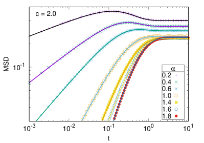
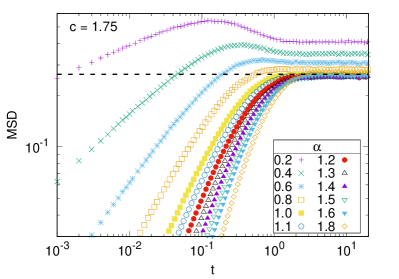
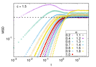
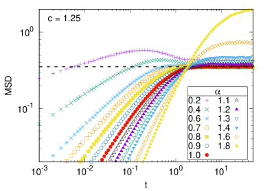
Figure 1: MSD for the potential scaling exponents $c=2.0$, $1.75$, $1.5$, and $1.25$, each shown for different anomalous diffusion exponents $\alpha$. The solid lines in the top left panel show the theoretical MSD (13) in the harmonic case. The horizontal dashed lines show the theoretically predicted stationary MSD (12) in the Brownian case.

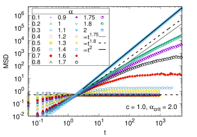
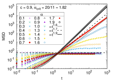
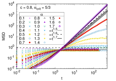
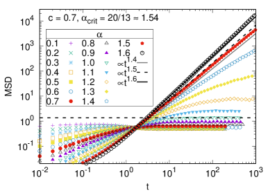
Figure 2: MSD for $c=1.0$, $0.9$, $0.8$, and $0.7$, each for different $\alpha$. The lines show the growth of the MSD of free FBM ($\propto t^{\alpha}$ with arbitrary prefactors), see the keys. The horizontal dashed lines show the theoretical stationary MSD (12) in the Brownian case.

3.3.1 MSD.

Figures 1 and 2 show the MSD for fixed scaling exponent $c>1$ and $c\leq 1$, respectively, each for different values of the FGN-exponent $\alpha$. According to our conjecture (10) as long as $c>1$ stationary states should exist for all values of $\alpha\leq 2$. As can be seen in figure 1 the MSD indeed clearly converges to a stationary value for all $c$ and $\alpha$. We also note that our simulation results agree well with the theory in the Brownian and harmonic cases, given by expressions (12) and (13).

For $c=1$ stationary states should exist for all $\alpha<\alpha_{\mathrm{crit}}=2$, whereas in the ballistic limit $\alpha=2$, no stationary state should exist. As demonstrated by the top left panel for $c=1$ in figure 2 the MSD reaches stationarity for FGN-exponents up to $\alpha=1.7$. For $\alpha$-values in the range $1.7<\alpha<2$ stationarity is not fully reached. We attribute this to an increasingly slower convergence to stationarity for larger $\alpha$, as the comparison to the growth of the MSD of the corresponding free FBM ($\propto t^{\alpha}$) clearly shows a decelerating growth of the MSD when the external potential is present. In contrast, in the ballistic limit, for which no stationary state should exist, the MSD grows perfectly proportional to that of free ballistic motion ($\propto t^{2}$) without any slowing-down.

For $c<1$ stationary states should exist for all $\alpha<\alpha_{\mathrm{crit}}=2/(2-c)$ and should not exist for $\alpha\geq\alpha_{\mathrm{crit}}$. Here, as shown in figure 2 our observation on the existence of stationary states is analogous to the case $c=1$. Namely, for smaller $\alpha$ values the MSD clearly reaches stationarity. For larger $\alpha$ values, that still fulfil the criterion $\alpha<\alpha_{\mathrm{crit}}$ but get close to the conjectured critical value $\alpha_{\mathrm{crit}}$ the convergence to stationarity becomes increasingly slow and stationarity is not fully reached. Again, the comparison to the growth of the MSD of the corresponding free FBM ($\propto t^{\alpha}$) clearly shows a decelerating growth of the MSD in those cases, whereas for $\alpha\geq\alpha_{\mathrm{crit}}$, for which no stationary states should exist, the growth of the MSD does not decelerate and is proportional or even a bit faster than for the corresponding free FBM. The effect that the observed motion in the presence of the potential accelerates slightly and eventually catches up with the MSD of the corresponding free FBM may be understood as follows: initially the particle strongly responds to the confining potential. Later, when the particle moves away from the origin and experiences a decreasing restoring force, it more and more moves like a free particle.

Figure 3 shows the MSD for fixed $\alpha$ and different values of the scaling exponent $c$ of the external potential. For $\alpha\leq 1$ stationary states should exist for all $c>0$, while for $\alpha>1$, they should exist only for $c>c_{\mathrm{crit}}=2(1-1/\alpha)$. As can be seen in the figure our simulation results are in agreement with this conjecture, despite the fact that for $c$ close to the critical value $c_{\mathrm{crit}}$ the convergence to stationarity becomes increasingly slow. We emphasise particularly the clear corroboration of our conjecture in the ballistic limit $\alpha=2$, for which the critical value is $c_{\mathrm{crit}}=1$ (see bottom right panel in figure 3).

On top of our discussion of the MSD with regards to the conjecture on the existence of stationary states, we address some additional properties of the MSD. First we note that the time to reach stationarity increases with $\alpha$ (as seen in figures 1 and 2) and decreases with $c$ (see figure 3). For instance, for $c=1.25$ stationarity is reached at around $t=5$ for $\alpha=1$, while for $\alpha=1.6$ it is reached at around $t=20$ (see figure 1). Likewise, for $\alpha=0.6$ stationarity is reached at around $t=2$ for $c=2$, while for $c=0.5$ it is reached at around $t=10$ (see figure 3). With respect to the dependence on $\alpha$ ($c$), this effect is more pronounced for smaller $c$ (larger $\alpha$).

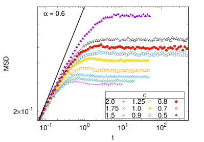
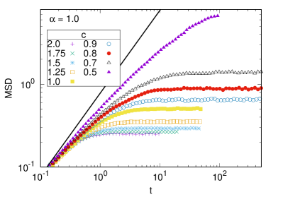
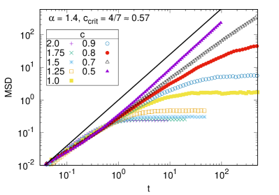
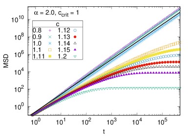
Figure 3: MSD for $\alpha=0.6$, $1.0$, $1.4$, and $2.0$, each for different $c$. The solid black lines show the growth of the MSD of the corresponding free FBM ($\propto t^{\alpha}$ with arbitrary prefactor).

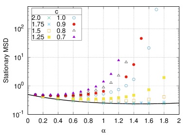
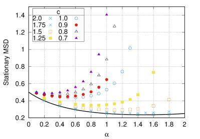
Figure 4: Stationary MSD as function of $\alpha$. The values were determined from the time-dependent MSD by averaging over the plateau regime. The black line shows the theoretical prediction (15) in the harmonic case. Left: log-lin scales, Right: lin-lin scales (not all data points shown).

The values of the MSD at stationarity as functions of the exponents $\alpha$ and $c$ are determined from averaging over the plateau regime of the time dependent MSD. Figure 4 shows the stationary MSD as function of $\alpha$. As can be seen the stationary MSD is not monotonic in $\alpha$: for $\alpha\leq\alpha_{0}$ it decreases with $\alpha$, while for $\alpha\geq\alpha_{0}$ it increases with $\alpha$. Here $\alpha_{0}$ is the value, which separates these two regimes. The value $\alpha_{0}$ increases with $c$, for instance, we have $\alpha_{0}(c=0.8)\approx 0.4$ and $\alpha_{0}(c=1.25)\approx 0.9$ (see the right panel of figure 4). We note that this non-monotonic behaviour is already present in the harmonic case and is in agreement with the theoretical prediction (15). Conversely, the stationary MSD is monotonically decreasing with $c$, as one would intuitively expect (see figure 3). This property can also be seen from figure 12 in the appendix which shows the stationary MSD as function of $c$.

We finally mention the "overshooting" of the MSD before reaching stationarity for smaller $\alpha$ values ($\alpha<1$). This phenomenon is already present in the harmonic case (see figure 1) and is also encoded in the analytical result (13), see also the discussion in [10, 11]. For $\alpha\geq 1$ and small $c$ (see figure 3) this effect is not observed.

3.3.2 PDF

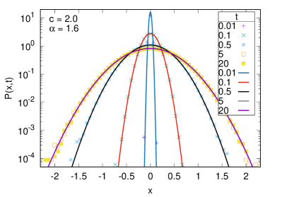
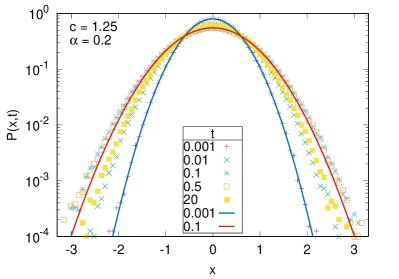
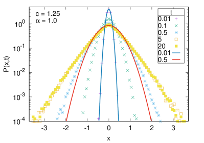
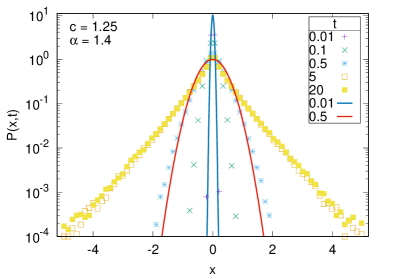
Figure 5: Time-dependent PDF for the cases $c=2$ (harmonic potential, top left panel) and $c=1.25$ for different $\alpha$ (remaining panels). The solid lines show the corresponding theoretical PDF (21) in the harmonic case. Note that the width of the PDF for $c=1.25$ and $\alpha=0.2$ initially increases (until approximately the curves for $t=0.1$ and $0.5$) and then decreases ($t=20$). This corresponds to the above-mentioned "overshooting" of the MSD (compare with the corresponding MSD in figure 1).

We now turn to the analysis of the PDF. Before addressing the stationary PDF, figure 5 shows as example the time-dependent PDF for the harmonic case $c=2$ and $c=1.25$. The simulation results agree well with the theoretical Gaussian PDF (21). For the non-harmonic potentials with $c>1$ the PDF agrees with the solution in the harmonic case at short times, an expected behaviour as long as the particle does not yet fully engage with the external potential. After this initial behaviour the PDF starts to deviate, and for persistent noise ($\alpha>1$) the PDF clearly assumes pronouncedly non-Gaussian shapes at long times.

Before analysing the stationary PDF in detail, some words about the convergence to stationarity are in order. In our numerical analysis we approximate the stationary PDF by the PDF taken at the longest simulated time $t_{\mathrm{max}}$, i.e., we take $P_{\mathrm{st}}(x)\approx P(x,t_{\mathrm{max}})$. For this approximation to be meaningful we determined the time $t_{\mathrm{st}}$ to reach stationarity as the earliest time when the MSD reaches stationarity and ensured that $t_{\mathrm{max}}\geq t_{\mathrm{st}}$. Following this procedure, in our analysis of the stationary PDF we limit ourselves to those parameter values of $\alpha$ and $c$ for which stationarity is fully reached in the simulations.

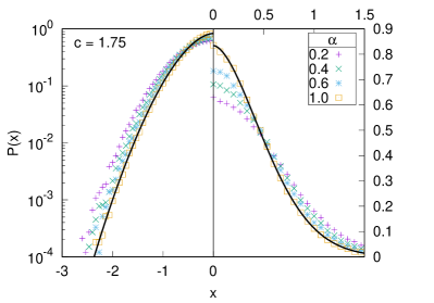
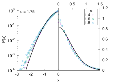
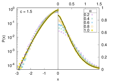
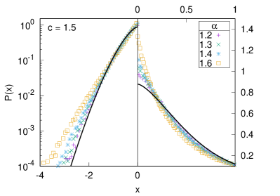
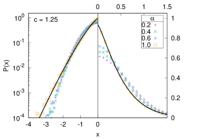
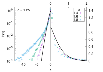
Figure 6: Stationary PDF for $c=1.75$, $1.5$, and $1.25$, each shown for different $\alpha$. For comparison, the black lines show the corresponding theoretical stationary PDF (11) in the Brownian case. Since the stationary PDF is symmetric about the $y$-axis, for $x<0$ the data (including the theoretical PDF) are plotted logarithmically (left and bottom axes in each panel) and for $x>0$ linearly (right and top axes).

Figures 6 and 7 show the stationary PDF for fixed $c>1$ and $c\leq 1$, respectively, each for different values of $\alpha$. Figure 8 shows the stationary PDF for fixed $\alpha$ and different $c$. First we note that the discussed non-monotonicity of the stationary MSD on $\alpha$ (section 3.3.1) is reflected in the width of the stationary PDF, although this effect is only slightly visible in the plots for $c=1.75$ and $1.5$, if one takes the full width at half of the maximum value of the PDF as a measure for the MSD (see figure 6 for the PDF and figure 1 for the MSD).

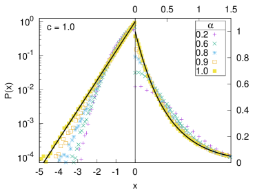
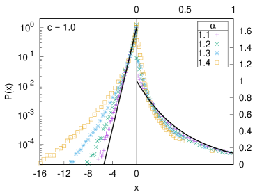
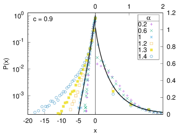
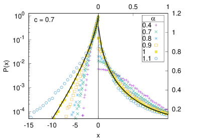
Figure 7: Stationary PDF for $c=1.0$, $0.9$, and $0.7$, each for different $\alpha$. For comparison, the black lines show the corresponding theoretical stationary PDF (11) in the Brownian case. For $x<0$ the data (including the theoretical PDF) are plotted logarithmically (left and bottom axes) and for $x>0$ linearly (right and top axes).

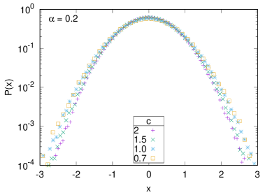
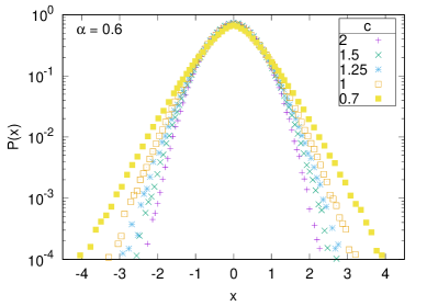
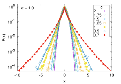
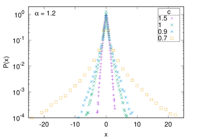
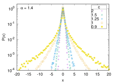
Figure 8: Stationary PDF for $\alpha=0.6$, $1.0$, $1.2$, and $1.4$, each for different $c$ values. The solid lines in the plot for $\alpha=1$ show the theoretical stationary PDF (11) and are in good agreement with the simulation results.

Next let us examine the tails of the stationary PDF. As can be seen in figures 6 and 7, for the case of persistent noise ($\alpha>1$) the tails decay slower than in the Brownian case, and for anti-persistent noise ($\alpha<1$), although less distinct at larger $c$ values, they decay faster than in the Brownian case. Generally, the decay becomes slower with increasing $\alpha$. With respect to $c$ the tails decay faster with increasing $c$, as one would expect, see figure 8.

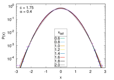
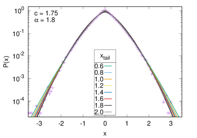
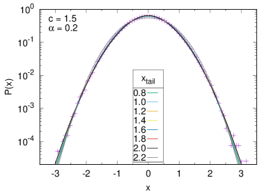
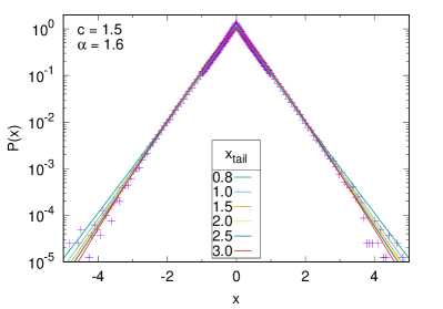
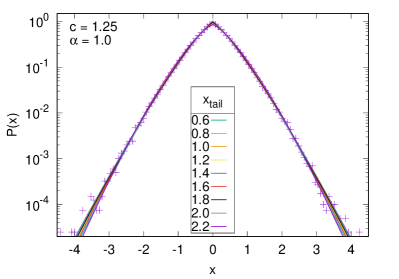
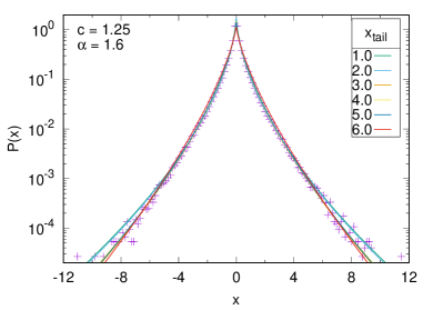
Figure 9: Fit of the tails ($|x|>x_{\mathrm{tail}}$) of the stationary PDF with the generalised exponential function (22) with fit parameters $a_{1}$ and $a_{2}$, for potential scaling exponents $c=1.75$, $1.5$, and $1.25$, and different $\alpha$.

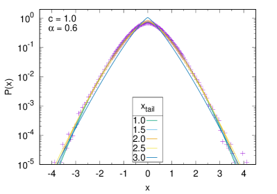
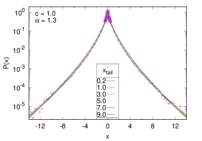
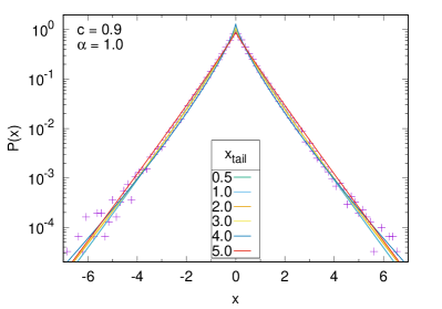
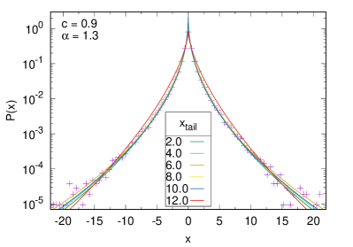
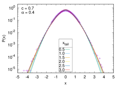
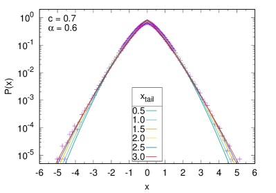
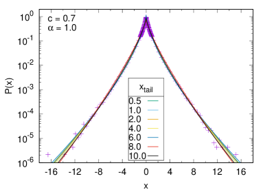
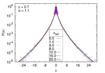
Figure 10: Fits of the tails ($|x|>x_{\mathrm{tail}}$) of the stationary PDF with the generalised exponential function (22) with fit parameters $a_{1}$ and $a_{2}$, for potential scaling exponents $c=1.0$, $0.9$, and $0.7$, and different $\alpha$.

Before we discuss these results further, we introduce the two-sided generalised exponential PDF

$$f(x)=\frac{1}{\mathscr{N}}e^{-a_{1}|x|^{a_{2}}},\qquad\mathscr{N}=\frac{2\Gamma(1/a_{2})}{{a_{1}}^{1/a_{2}}a_{2}},$$ (22)

with the parameters $a_{1},a_{2}>0$. It encompasses the stationary PDF in the Brownian (expression (11)) and harmonic (expression (20)) cases with $a_{1}=1/K$ and $a_{1}=2^{\alpha-1}/[K\Gamma(1+\alpha)]$, respectively, and $a_{2}=c$ is given by the potential shape. Figures 9 and 10 show the fits of the tails ($|x|\geq x_{\mathrm{tail}}$) of the stationary PDF with the generalised exponential fit function (22) and fit-parameters $a_{1}$ and $a_{2}$. Our analysis shows that the fit parameters are quite robust with respect to the precise choice for $x_{\mathrm{tail}}$. As can be seen, the agreement with the fit function is quite nice for larger potential scaling exponents $c$ and smaller FGN exponent $\alpha$.

Due to the symmetry of the PDF (22), the first moment is zero, and for the second and fourth moments we find

$$\langle X^{2}\rangle ={a_{1}}^{-2/a_{2}}\frac{\Gamma(3/a_{2})}{\Gamma(1/a_{2})},$$ (23)

$$\langle X^{4}\rangle ={a_{1}}^{-4/a_{2}}\frac{\Gamma(5/a_{2})}{\Gamma(1/a_{2})}.$$ (24)

Hence, the kurtosis becomes

$$\kappa=\frac{\langle(X-\langle X\rangle)^{4}\rangle}{\langle(X-\langle X\rangle)^{2}\rangle^{2}}=\frac{\Gamma(5/a_{2})\Gamma(1/a_{2})}{\Gamma^{2}(3/a_{2})}.$$ (25)

Note that $\kappa$ is independent of the parameter $a_{1}$, and in the Brownian and harmonic cases $a_{2}=c$.

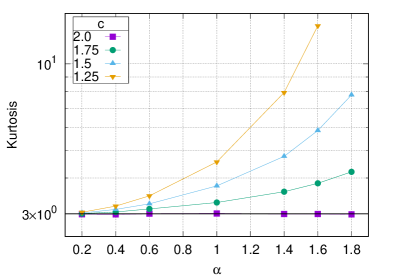
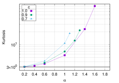
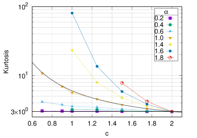
Figure 11: Kurtosis calculated from the simulated stationary PDF as function of $\alpha$ (top) and $c$ (bottom). The horizontal lines show the kurtosis value of 3 for a Gaussian, the grey line shows the theoretical value of the kurtosis in the Brownian case for different $c$ values, expression (25) with $a_{2}=c$.

Figure 11 shows the kurtosis, determined from the numerical simulations, as function of $\alpha$ (top panels) and $c$ (bottom panel). This measured kurtosis agrees well with the theoretical prediction in the Brownian and harmonic cases (equation (25)). The kurtosis $\kappa$ monotonically increases with $\alpha$ and decreases with $c$, which corresponds to the fact that the tails of the stationary PDF fall off slower in $|x|$ with increasing $\alpha$ (increasing persistence) and faster with increasing $c$. Moreover, compared to the Brownian case ($\alpha=1$) the kurtosis is larger for persistent noise ($\alpha>1$) and smaller for anti-persistent noise ($\alpha<1$), which is consistent with the slower decay in $|x|$ of the tails for $\alpha>1$ (and faster for $\alpha<1$), as compared to the Brownian case.

We note that for all $c\neq 2$ the stationary PDF is leptokurtic, i.e., has "fatter" tails with $\kappa>3$, and approaches the Gaussian value of 3 for $c\to 2$. Interestingly, for small $\alpha$ values the kurtosis stays close to the Gaussian value of 3, and in fact converges to it for $\alpha\to 0$, independent of $c$ (see top panels in figure 11). This result is consistent with figure 8, where larger $\alpha$-values produce strongly leptokurtic PDFs and smaller $\alpha$ values lead to more Gaussian shapes, compare also A.

4 Conclusion

FBM is a strongly non-Markovian stochastic process. Despite the stationary increments, the long-ranged, power-law noise auto-correlation leads to distinct effects of (anti-)persistence, which, in turn, lead to a number of properties for which FBM defies analytical approaches. A long-standing example is the lack of direct analytical methods to calculate the first-passage dynamics of FBM, for which only asymptotic [47], numerical [48, 42], or perturbative [49] approaches exist. This is related to the fact that, for instance, the seemingly simple Fokker-Planck equation (16) in the harmonic case or in absence of an external potential, cannot be used to formally derive the boundary value solution for a semi-infinite or finite domain with reflecting boundaries [48, 42]. Even more so, numerical studies show that the PDF of FBM next to reflecting boundaries is not flat but shows accretion or depletion next to the boundaries for persistent or anti-persistent cases [24, 50, 51, 52], with potential implications to the growth density of serotonergic brain fibres [53]. Another remarkable phenomenon was observed for FGN-driven motion subject to a fluctuation-dissipation relation governed by the fractional Langevin equation. In this case a critical exponent was found at which a harmonically bound particle switches between a non-monotonic underdamped phase and a "resonance" phase, in the presence of an external sinusoidal driving [54]. In many cases, therefore, to explore the detailed properties of FBM one needs to resort to numerical analyses.

Based on the overdamped Langevin equation driven by FGN, we here studied in detail the stochastic motion of FBM in a subharmonic potential by examining the MSD and PDF. The most striking result we obtained is the conjecture that there exists a long-time stationary state if the relation $c>2(1-1/\alpha)$ is satisfied. We corroborated this conjecture via numerical analysis of FBM for a wide range of potential scaling exponents $c$ and FGN-exponents $\alpha$. In particular, this implies that while for anti-persistent or uncorrelated FGN ($\alpha\leq 1$) there always exists a long-time stationary state for any $c>0$. For persistent FGN ($\alpha>1$) the competition between the confining tendency of the potential and the persistence of the motion turns out to become a delicate balance. This behaviour is analogous to what was found for the overdamped Langevin equation driven by white Lévy-stable noise [22]. In the Lévy-stable case, however, the confining tendency of the potential was in competition with the occasional, extremely long jumps due to the diverging second moment of the driving Lévy noise. Despite this fundamental difference in the dynamics of the two processes, in both cases the condition for the existence of stationarity can be written as $c>2-1/H$ where $H$ is the self-similarity index of the unconfined process. We note that the similarity between both FBM and Lévy flights also extends to superharmonic potentials, e.g., in the existence of multimodal states, see the discussion in [23]. We also note that superdiffusive FBM may explain similar features in the observed motion of searching and migrating birds as Lévy flights [55].

We also demonstrated that the time to reach stationarity increases with growing $\alpha$ and decreases with growing $c$. Moreover, the stationary MSD monotonically decreases with growing $c$, as intuitively expected. In dependence on $\alpha$, the behaviour of the stationary MSD is more complicated in that it is non-monotonic in $\alpha$. Namely for $\alpha\leq\alpha_{\mathrm{crit}}(c)$ it decreases with growing $\alpha$, while for $\alpha\geq\alpha_{\mathrm{crit}}(c)$ it increases with growing $\alpha$. The critical value $\alpha_{\mathrm{crit}}(c)$ increases monotonically with growing $c$.

In the analysis of the PDF we showed that at short times the behaviour is close to free motion or motion in an harmonic potential, before the particle engages with the confining potential. At stationarity the tails of the PDF decay faster with decreasing $\alpha$ and growing $c$. Particularly, for $\alpha>1$ ($\alpha<1$) the tails decay slower (faster) in $|x|$ than in the Brownian case. This is contrary to the case of FBM in a superharmonic potential ($c>2$), as detailed in [23]. We also showed that the two-sided generalised exponential PDF (22) provides a good description for the stationary PDF as long as $c$ is not too small and $\alpha$ not too large. Finally we showed that the stationary PDF is leptokurtic ("fat-tailed") for $c\neq 2$ and hence non-Gaussian. For the fully anti-persistent case $\alpha\to 0$ the kurtosis approaches the Gaussian value 3.

It will be interesting to see how this picture extends once the driving FGN is tempered in terms of an exponential or power-law cutoff [56]. Of course, in this case the long-term PDF beyond the cutoff time always has the Boltzmannian shape (11), however, the transient behaviour is expected to be quite rich. Such a scenario may be relevant for various processes in which cutoffs become relevant, e.g., finite system sizes or systems with finite correlation times, such as lipid motion in membrane bilayers [57]. We also mention the analysis of confinement effects for FBM with random parameters, see, e.g., [59, 58], or for particles with stochastically changing mobilities suspended in non-equilibrium viscoelastic liquids [60, 61, 62].

Appendix A Curvature of the stationary PDF and stationary MSD as function of $c$

Here we briefly allude to the classification of the stationary PDFs according to their shape. More precisely, we can divide the stationary PDFs into two distinct groups according to their curvature, by which we mean their second derivative. First, consider the Brownian case ($\alpha=1$) for which the stationary PDF is given by expression (11). A straightforward calculation shows that for $c\leq c_{\mathrm{cr}}(\alpha=1)=1$ the curvature is positive for all $x\neq 0$, while for $c>c_{\mathrm{cr}}(\alpha=1)=1$ the curvature changes sign at $|x|=x_{\mathrm{cr}}=((c-1)/(2c))^{1/c}$, such that the curvature is positive for $|x|>x_{\mathrm{cr}}$ and negative for $|x|<x_{\mathrm{cr}}$. Compare also the plot for $\alpha=1$ in figure 8.

In general, we observe that for all $\alpha$ there is a critical value $c_{\mathrm{cr}}(\alpha)$ such that for all $c\leq c_{\mathrm{cr}}(\alpha)$ the stationary PDFs exhibit a positive curvature for all $x\neq 0$, while for all $c>c_{\mathrm{cr}}(\alpha)$ the curvature has a change of sign at some $|x|=x_{\mathrm{cr}}(\alpha,c)>0$ such that the curvature is positive for $|x|>x_{\mathrm{cr}}$ and negative for $|x|<x_{\mathrm{cr}}$.

The critical value $c_{\mathrm{cr}}(\alpha)$ increases with $\alpha$. For instance, for $\alpha=1.8$ and $c=1.25$ the stationary PDF exhibits a positive curvature, while for $\alpha=1$ and $c=1.25$ the curvature of the stationary PDF changes sign. Also, for $\alpha=0.2$ and $c=0.7$ the curvature of the stationary PDF changes sign, while for $\alpha=1$ and $c=0.7$ the curvature of the stationary PDF is positive.

Finally, in figure 12 we show the stationary MSD as function of the potential scaling exponent $c$ for various $\alpha$, thus complementing figure 3 in the main text.

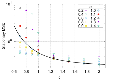
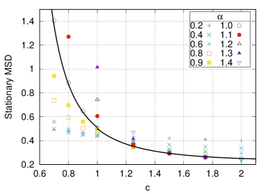
Figure 12: Stationary MSD as a function of $c$. The values were determined from the time-dependent MSD by averaging over the plateau regime. The black line shows the theoretical prediction (12) in the Brownian case. Left: log-lin plot, Right: lin-lin plot (not all all data points shown).

References

References

- [1] E. Kappler, Ann. Phys. (Leipzig) 11, 233 (1931).
- [2] L. D. Landau and E. M. Lifshitz, Landau and Lifshitz Course of Theoretical Physics 5: Statistical Physics Part 1 (Butterworth-Heinemann, Oxford UK, 1980).
- [3] D. A. Schafer, J. Gelles, M. P. Sheetz, and R. Landick, Nature 352, 444 (1991).
- [4] S. F. Tolic-Nørrelykke, M. B. Rasmussen, F. S. Savone, K. Berg-Sørensen, and L. B. Oddershede, Biophys. J. 90, 3694 (2006).
- [5] T. Franosch, M. Grimm, M. Belushkin, F. M. Mor, G. Foffi, L. Forró, and S. Jeney, Nature 478, 85 (2011).
- [6] E. M. Lifshitz and L. P. Pitaevski, Landau and Lifshitz Course of Theoretical Physics 10: Physical Kinetics (Butterworth-Heinemann, Oxford UK, 1981).
- [7] N. van Kampen, Stochastic processes in physics and chemistry (North Holland, Amsterdam, 1981).
- [8] W. T. Coffey and Y. P. Kalmykov, The Langevin equation (World Scientific, Singapore, 2012).
- [9] J.-H. Jeon, N. Leijnse, L. B. Oddershede, and R. Metzler, New J. Phys. 15, 045011 (2013).
- [10] J.-H. Jeon and R. Metzler, Phys. Rev. E 85, 021147 (2012).
- [11] J. Kursawe, J. Schulz, and R. Metzler, Phys. Rev. E 88, 062124 (2013).
- [12] R. Metzler, E. Barkai, and J. Klafter, Phys. Rev. Lett. 82, 3563 (1999).
- [13] R. Metzler and J. Klafter, Phys. Rep. 339, 1 (2000).
- [14] S. Burov, R. Metzler, and E. Barkai, Proc. Natl. Acad. Sci. USA 107, 13228 (2010).
- [15] S. Burov, J.-H. Jeon, R. Metzler, and E. Barkai, Phys. Chem. Chem. Phys. 13, 1800 (2011).
- [16] J.-H. Jeon, V. Tejedor, S. Burov, E. Barkai, C. Selhuber-Unkel, K. Berg-Sørensen, L. Oddershede, and R. Metzler, Phys. Rev. Lett. 106, 048103 (2011).
- [17] H. Yang, G. Luo, P. Karnchanaphanurach, T.-M. Louie, I. Reich, S. Cova, L. Xun, and X. S. Xie, Science 302, 262 (2003).
- [18] X. Hu, L. Hong, M. D. Smith, T. Neusius, X. Cheng, and J. C. Smith, Nature Phys. 12, 171 (2016).
- [19] A. Chechkin, V. Gonchar, J. Klafter, R. Metzler, and L. Tanatarov, Chem. Phys. 284, 233 (2002).
- [20] A. V. Chechkin, J. Klafter, V. Yu. Gonchar, R. Metzler, and L. V. Tanatarov, Phys. Rev. E 67, 010102(R) (2003).
- [21] A. A. Dubkov, B. Spagnolo, and V. V. Uchaikin, Int. J. Bifurc. Chaos 18, 2649 (2008).
- [22] K. Capała, A. Padash, A. V. Chechkin, B. Shokri, R. Metzler, and B. Dybiec, Chaos 30, 123103 (2020).
- [23] T. Guggenberger, A. Chechkin, and R. Metzler, J. Phys. A 54, 29LT01 (2021).
- [24] T. Guggenberger, G. Pagnini, T. Vojta, and R. Metzler, New J. Phys. 21, 022002 (2019).
- [25] I. M. Sokolov, Euro. J. Phys. 31, 1353 (2010).
- [26] P. S. Burada, G. Schmid, D. Reguera, J. M. Rubi, and P. Hänggi, Phys. Rev. E 75, 051111 (2007).
- [27] H. Risken, The Fokker-Planck equation (Springer, Heidelberg, 1989).
- [28] D. A. Kessler and E. Barkai, Phys. Rev. Lett. 105, 120602 (2010).
- [29] B. Dybiec, I. M. Sokolov, and A. V. Chechkin, J. Stat. Mech. 2010, P07008 (2010).
- [30] A. N. Kolmogorov, C. R. (Doklady) Acad. Sci. URSS (N.S.) 26, 115 (1940).
- [31] B. B. Mandelbrot and J.Van Ness, SIAM Rev. 10, 422 (1968).
- [32] H. Qian, in Processes with Long-Range Correlations, edited by G. Rangajaran and M. Z. Ding (Springer, Heidelberg, 2003).
- [33] P. E. Kloeden and E. Platen, Numerical Solution of Stochastic Differential Equations (Springer, Heidelberg, 1992).
- [34] T. Dieker, Simulation of fractional Brownian motion, MSc thesis, Vrije Universiteit Amsterdam, revised version (2004).
- [35] S. Jespersen, R. Metzler, and H. C. Fogedby, Phys. Rev. E 59, 2736 (1999).
- [36] H. C. Fogedby, Phys. Rev. Lett. 73, 2517 (1994).
- [37] H. C. Fogedby, Phys. Rev. E 58, 1690 (1998).
- [38] A. V. Chechkin, V. Yu. Gonchar, J. Klafter, R. Metzler, and L. V. Tanatarov, J. Stat. Phys. 115, 1505 (2004).
- [39] R. Metzler, E. Barkai, and J. Klafter, Europhys. Lett. 46, 431 (1999).
- [40] A. Weron and M. Magdziarz, Europhys. Lett. 86, 60010 (2009).
- [41] M. Abramowitz and I. A. Stegun, Handbook of Mathematical Functions (National Bureau of Standards, Bethesda, 1972)
- [42] O. Sliusarenko, V. Yu. Gonchar, A. V. Chechkin, I. M. Sokolov, and R. Metzler, Phys. Rev. E 81, 041119 (2010).
- [43] R. Zwanzig, Nonequilibrium statistical mechanics (Oxford University Press, Oxford, UK, 2001).
- [44] Yu. L. Klimontovich, Turbulent motion and the structure of chaos (Kluwer, Dordrecht, 1991).
- [45] S. A. Adelman, J. Chem. Phys. 64, 124 (1976).
- [46] P. Hänggi and P. Jung, Colored Noise in Dynamical Systems (John Wiley, New York, 1994)
- [47] G. M. Molchan, Commun. Math. Phys. 205, 97 (1999).
- [48] J.-H. Jeon, A. V. Chechkin, and R. Metzler, Europhys. Lett. 94, 20008 (2011).
- [49] K. J. Wiese, S. N. Majumdar, and A. Rosso, Phys. Rev. E 83, 061141 (2011).
- [50] A. H. O. Wada and T. Vojta, Phys. Rev. E 97, 020102(R) (2018).
- [51] T. Vojta, S. Skinner, and R. Metzler, Phys. Rev. E 100, 042142 (2019).
- [52] T. Vojta, S. Halladay, S. Skinner, S. Janušonis, T. Guggenberger, and R. Metzler, Phys. Rev. E 102, 032108 (2020).
- [53] S. Janušonis, N. Detering, R. Metzler, and T. Vojta, Frontiers Comp. Neurosci. 14, 56 (2020).
- [54] S. Burov and E. Barkai, Phys. Rev. Lett. 100, 070601 (2008).
- [55] O. Vilk, E. Aghion, T. Avgar, C. Beta, O. Nagel, A. Sabri, R. Sarfati, D. K. Schwartz, M. Weiss, D. Krapf, R. Nathan, R. Metzler, and M. Assaf, E-print arXiv:2109.04309.
- [56] D. Molina-Garcia, T. Sandev, H. Safdari, G. Pagnini, A. Chechkin, and R. Metzler, New J. Phys. 20, 103027 (2018).
- [57] J.-H. Jeon, H. Martinez-Seara Monne, M. Javanainen, and R. Metzler, Phys. Rev. Lett. 109, 188103 (2012).
- [58] W. Wang, F. Seno, I. M. Sokolov, A. V. Chechkin, and R. Metzler, New J. Phys. 22, 083041 (2020).
- [59] A. Sabri, X. Xu, D. Krapf, and M. Weiss, Phys. Rev. Lett. 125, 058101 (2020).
- [60] E. Yamamoto, T. Akimoto, A. Mitsutake, and R. Metzler, Phys. Rev. Lett. 126, 128101 (2021).
- [61] F. Baldovin, E. Orlandini, and F. Seno, Frontiers Phys. 7, 124 (2019).
- [62] M. Hidalgo-Soria and E. Barkai, Phys. Rev. E 102, 012109 (2020).