Emergent space-time supersymmetry at disordered quantum critical points

Abstract

We study the effect of disorder on the spacetime supersymmetry that is proposed to emerge at the quantum critical point of pair density wave transition in (2+1)D Dirac semimetals and (3+1)D Weyl semimetals. In the (2+1)D Dirac semimetal, we consider three types of disorder, including random scalar potential, random vector potential and random mass potential, while the random mass disorder is absent in the (3+1)D Weyl semimetal. Via a systematic renormalization group analysis, we find that any type of weak random disorder is irrelevant due to the couplings between the disorder potential and the Yukawa vertex. The emergent supersymmetry is thus stable against weak random potentials. Our work will pave the way for exploration supersymmetry in realistic condensed matter systems.

I Introduction

About five decades ago, the spacetime supersymmetry (SUSY) was proposed as a possible way of solving the hierarchy problem of the standard model [1, 2, 3, 4] and the cosmological constant problem[5]. Later, some supersymmetric theories have been studied as toy models to understand strong coupling physics rigorously [6, 7]. Due to these attractive features, SUSY has been studied intensively in past fifty years and there is some expectation before that SUSY may be revealed in the large hadron collider (LHC). Unfortunately, the recent experiments at the LHC have found no evidence of SUSY and/or its spontaneous breaking in particle physics.

Three-dimensional (3D) Weyl fermions [8, 9, 10] in noncentrosymmetric materials [11, 12, 13, 14, 15] provide an opportunity to test and investigate important concepts developed in the context of high-energy physics in realistic condensed matter systems. It has been suggested that SUSY can emerge in the low-energy limit of a number of non-supersymmetric models [16, 17, 18, 19, 20, 21, 22, 23, 24, 25, 26]. In particular, SUSY is proposed to emerge at quantum critical points (QCPs) in Bose-Fermi lattice models [27, 28], in the (2+1)D surface states of topological insulators [29, 30, 31, 32, 33], as well as at multicritical points in some low-dimensional systems [34, 35, 36]. Moreover, an interesting recent suggestion [37] is that SUSY can be realized at certain pair-density-wave (PDW) superconducting quantum critical points of ideal Weyl semimetals [38, 39](WSMs).

The realization of SUSY at QCPs relies crucially on the fact that the infrared fixed point is stable against small perturbations. In particular, for the emergent SUSY to be realized, it must be robust when the fermions are subject to small perturbations from quenched disorder and other dissipation effects. Here, we are particularly interested in the impact of quenched disorder on the emergent SUSY, because disorder unavoidably exists in all realistic materials. It is well known that disorder plays an essential role in condensed matter systems [40, 41, 42, 43, 44, 45, 46, 47, 48]and may lead to a plenty of prominent phenomena, such as Anderson localization and metal-insulator transition. In graphene-like Dirac semimetals (DSMs), depending on the specific type, disorder can either enhance or reduce the effective Coulomb interaction strength [49, 50, 51, 52, 53, 54, 55], which in turn drastically modifies the phase diagram obtained in the clean limit [49, 50, 51, 52, 53, 54, 55]. Moreover, disorder may have a significant impact on the low-temperature properties of various Dirac or Weyl semimetals, such as the conductivity of graphene [56, 50, 57, 58], the optical conductivity of WSMs [59], and the low-energy spectral, thermodynamic, and transport behaviors of $d$-wave cuprate superconductors [60, 45, 61, 62, 63]. Disorder also plays a vital role in quantum Hall systems [64, 65, 66, 67] and topological insulators [29, 30].

In this paper, we investigate the stability of emergent SUSY against the disorder scattering. We focus on the disorder-induced unusual renormalization of the fermion velocity [53, 62, 68], and examine whether such a renormalization effect causes a substantial difference between the velocities of fermions and bosons at low energies, and ruins the emergent SUSY. Based on this analysis, we are able to identify the influence of non-magnetic disorder on the particular fixed point that is argued to display an emergent SUSY at the QCP of pair density wave (PDW) transition in (3+1)D WSMs and (2+1)D DSMs [37]. In the case of (2+1)D DSMs, we consider three types of disorder, including random scalar potential (RSP), random vector potential (RVP), and random mass (RM). In (2+1)D, our systematic RG analysis reveals that weak RVP, RMP and RSP are irrelevant at the QCPs where fermion velocity and boson velocity flow into same value under renormalization, which certainly does not breaks the emergent SUSY. In (3+1)D WSMs, the disorder potential becomes more irrelevant and the effective SUSY is robust against weak disorder. The schematic RG flow diagram for emergent SUSY is shown in Fig.1

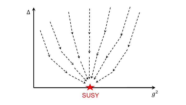
Figure 1: Schematic RG flow near SUSY fixed point as a function the Yukawa coupling $g^{2}$ and quench disorder strength $\Delta$. The emergent SUSY fixed point is stable for weak random quench disorders from our one-loop level RG calculations.

This paper is structured as follows. In Sec. II, we present the effective model for (2+1)D disordered DSMs and perform the RG calculations. In Sec. III, the same analysis is carried out in (3+1)D WSMs. We briefly summarize the results of this work in Sec. IV. Further RG details for our calculations are provided in Appendix.

II (2+1)D Dirac semimetals

As demonstrated in Ref. [37], a spactime SUSY could emerge in the low-energy region at the PDW QCP of (2+1)D DSMs only when the number of massless Dirac fermions is $N_{f}=2$. In this case, the low-energy effective action at the PDW criticality in a clean system is given by

$$S = S_{f}+S_{b}+S_{I},$$ (1)

$$S_{f} = \int d^{2}xd\tau\sum_{n=\pm}\psi_{n}^{\dagger}\Big{[}\partial_{\tau}+iv_{f}\sum_{j=1}^{2}\gamma_{j}\partial_{j}\Big{]}\psi_{n},$$ (2)

$$S_{b} = \int d^{2}xd\tau\bigg{\{}\sum_{n=\pm}\Big{[}|\partial_{\tau}\phi_{n}|^{2}+v_{b}^{2}\sum_{j=1}^{2}|\partial_{j}\phi_{n}|^{2}$$

$$+r|\phi_{n}|^{2}+u|\phi_{n}|^{4}\Big{]}+u_{+-}|\phi_{1}|^{2}|\phi_{2}|^{2}\bigg{\}},$$

$$S_{I} = \int d^{2}xd\tau g\sum_{n=\pm}\Big{[}\phi_{n}\psi_{n}^{T}\sigma_{y}\psi_{n}+h.c.\Big{]},$$ (4)

where $\gamma_{j}=(\sigma_{x},\sigma_{y})$. $\sigma_{\alpha},\alpha=x,y$ is Pauli matrix with spin indices. $S_{f}$ corresponds to the action for two non-interacting two-component Dirac fermions $\psi_{\pm}$ at two Dirac points $\bm{Q}_{\pm}$ [69, 70], with quartic and higher order self-coupling terms being irrelevant [27] at low energies. $S_{b}$ describes the quantum fluctuation and the self-coupling of the PDW order parameter $\phi_{n}$ near the QCP, where $\phi_{\pm}$ is the superconducting order with momentum $2\bm{Q}_{\pm}$, respectively. Terms with higher powers of $\phi_{n}$ are all irrelevant, whereas $\phi_{n}^{\ast}\partial_{\tau}\phi_{n}$ is excluded by particle-hole symmetry [37]. $S_{I}$ represents the Yukawa coupling between Dirac fermions and bosons. The terms of the form $\phi_{-}^{\ast}\psi_{+}{\sigma}_{y}\psi_{+}$ and $\phi_{-}^{\ast}\psi_{+}{\sigma}_{y}\psi_{-}$ are not allowed because they do not satisfy momentum conservation [27]. Therefore, the effective action given above is of the most general form. It has been shown through renormalization group analysis that an emergent spacetime SUSY occurs at the low energy limit. A necessary condition for the emergent SUSY is that velocities of fermions and bosons flow to the same value under RG, which renders the emergent Lorentz symmetry. It was claimed that such an emergent Lorentz symmetry can be naturally realized in a number of correlated electron systems [27, 28, 37, 29, 30, 31, 32, 33].

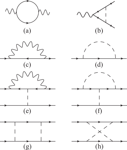
Figure 2: Feynman diagrams for all the relevant one-loop diagrams that survive within replica limit. Here, the solid line represents the free fermion propagator, the wavy line the free boson propagator, and the dashed line the disorder.

The aim of the present work is to examine whether the emergent SUSY is robust against disorder scattering. For this purpose, we now introduce a direct fermion-disorder coupling term to the system via the standard form, also see Appendix A [67, 71, 45, 49, 50, 51, 63, 53],

$$S_{\mathrm{dis}}=\int d^{2}xd\tau\sum_{n=\pm}\psi_{n}^{\dagger}\left(\sum_{\Gamma}V_{\Gamma}(\mathbf{x})\Gamma\right)\psi_{n},$$ (5)

where $V_{\Gamma}(\mathbf{x})$ stands for the random potential and $\Gamma$ labels the type of the disorder potential. We assume $V_{\Gamma}(\mathbf{x})$ to be a quenched, Gaussian white noise potential characterized by the following identities:

$$\langle V_{\Gamma}(\mathbf{x})\rangle=0,\quad\langle V_{\Gamma}(\mathbf{x})V_{\Gamma^{\prime}}(\mathbf{x}^{\prime})\rangle=\Delta_{\Gamma}\delta_{\Gamma\Gamma^{\prime}}\delta(\mathbf{x}-\mathbf{x}^{\prime}),$$ (6)

where $\langle...\rangle$ denotes average over disorder distribution and $\Delta_{\Gamma}$ is introduced to characterize the strength of random potential.

We consider three different types of disorder classified by the different matrices $\Gamma$. In particular, $\Gamma=\mathbb{I}_{2\times 2}$ for RSP, $\Gamma=\sigma_{z}$ for RM, and $\Gamma=(\sigma_{x},\sigma_{y})$ for RVP. These three types are most frequently studied in the literature and they can be induced by some specific mechanisms in realistic materials [71, 72, 73, 74, 75, 76, 77]. These three types of random potential might exist individually, or coexist in the same material. To be general, we assume that they coexist in the system and analyze their impact by performing RG calculations.

The random potential $V(\mathbf{x})$ can be properly averaged by employing the replica trick [40, 78, 52, 54, 79, 59], which leads us to an interacting effective action of short-range fermion-fermion interaction:

$$S_{\mathrm{dis}}= -\frac{1}{2}\int d^{2}xd\tau d\tau^{\prime}\Big{\{}\sum_{n=\pm}\Big{[}\Delta_{S}\big{(}\psi_{n}^{\dagger\alpha}\psi_{n}^{\alpha}\big{)}_{x}\big{(}\psi_{n}^{\dagger\beta}\psi_{n}^{\beta}\big{)}_{x^{\prime}}+\Delta_{M}\big{(}\psi_{n}^{\dagger\alpha}{\sigma}_{z}\psi_{n}^{\alpha}\big{)}_{x}\big{(}\psi_{n}^{\dagger\beta}{\sigma}_{z}\psi_{n}^{\beta}\big{)}_{x^{\prime}}$$

$$+\Delta_{V}\sum_{j}\big{(}\psi_{n}^{\dagger\alpha}{\sigma}_{j}\psi_{n}^{\alpha}\big{)}_{x}\big{(}\psi_{n}^{\dagger\beta}{\sigma}_{j}\psi_{n}^{\beta}\big{)}_{x^{\prime}}\Big{]}+2\Delta_{S}^{\prime}\big{(}\psi_{+}^{\dagger\alpha}\psi_{+}^{\alpha}\big{)}_{x}\big{(}\psi_{-}^{\dagger\beta}\psi_{-}^{\beta}\big{)}_{x^{\prime}}$$

$$+2\Delta_{M}^{\prime}\big{(}\psi_{+}^{\dagger\alpha}{\sigma}_{z}\psi_{+}^{\alpha}\big{)}_{x}\big{(}\psi_{-}^{\dagger\beta}{\sigma}_{z}\psi_{-}^{\beta}\big{)}_{x^{\prime}}+2\Delta_{V}^{\prime}\sum_{j}\big{(}\psi_{+}^{\dagger\alpha}{\sigma}_{j}\psi_{+}^{\alpha}\big{)}_{x}\big{(}\psi_{-}^{\dagger\beta}{\sigma}_{j}\psi_{-}^{\beta}\big{)}_{x^{\prime}}\Big{\}}$$ (7)

where $j=(x,y)$, $\alpha$ and $\beta$ are the replica indices, $x\equiv(\mathbf{x},\tau)$ and $x^{\prime}\equiv(\mathbf{x},\tau^{\prime})$ are the space-time coordinate. The repeated indices $\alpha$ and $\beta$ are summed automatically. In the replica theory, the replica limit $\sum_{\alpha}=N\rightarrow 0$ is implemented in the following RG calculation. Three parameters $\Delta_{S}$, $\Delta_{M}$, and $\Delta_{V}$ characterize the effective strength of quartic couplings of Dirac fermions induced by averaging over RS, RM, and RVP, respectively. The two pieces of Dirac fermions share the same random potential. Three cross terms characterized by $\Delta_{S}^{\prime}$, $\Delta_{M}^{\prime}$, and $\Delta_{V}^{\prime}$ are induced in the replica limit. In the RG analysis, the bare values of the parameters are the same, $\Delta_{S}^{\prime 0}=\Delta_{S}^{0}$, $\Delta_{M}^{\prime 0}=\Delta_{M}^{0}$, and $\Delta_{V}^{\prime 0}=\Delta_{V}^{0}$, moreover, the RG equations for $\Delta_{\Gamma}$ and $\Delta_{\Gamma^{\prime}}$ are the same (see Appendix B for details), so we focus on $\Delta_{\Gamma}$ in the following.

As shown in previous calculations [53, 62, 68], disorder can strongly affect the RG flow of fermion velocity as the energy is lowered. If the disorder coupling is relevant that flow to a finite value at low energy limit, it will drive the fermion velocity to vanish at sufficiently low energies, which then spoils the Lorentz symmetry for the fermion sector, but not for the boson sector. As a result, the emergent Lorentz symmetry, and thus the emergent SUSY will be ruined by disorder. However, whether this takes place relies crucially on the scale dependence of disorder coupling parameter. In the case of (2+1)D DSMs, naive power-counting, according to Eqs. (2) and (7), shows that disorder is marginal. A careful analysis of the marginal disorder effect is helpful to tell us whether a irrelevant and a relevant coupling need to investigate further.

To this end, we carry out a detailed RG analysis starting from the critical action with $r=0$, represented by Eq. (1) along with Eq. (7), by considering the leading order of the $\epsilon$-expansion, where $\epsilon=4-D=3-d$, $D$ and $d$ are the spacetime dimension and the spatial dimension, respectively. The pertinent one-loop Feynman diagrams are shown in Fig. 2. After integrating out the fast modes defined within the momentum shell $e^{-l}\Lambda<|\mathbf{p}|<\Lambda$ and then performing RG transformations [80], we obtain the following RG equations (the detailed results are presented in appendix)

$$\frac{dv_{f}}{dl} =v_{f}\Big{[}g^{2}(G_{1}-G_{0})-2\sum_{\Gamma}\Delta_{\Gamma}\Big{]},$$ (8)

$$\frac{da}{dl} =g^{2}\Big{(}\frac{1-a^{2}}{2a}+a(G_{0}-G_{1})\Big{)}+2a\sum_{\Gamma}\Delta_{\Gamma},$$ (9)

$$\frac{dg^{2}}{dl} =\epsilon g^{2}-g^{4}\big{(}1-G_{0}+3G_{1}\big{)}+\big{(}4\Delta_{S}+2\sum_{\Gamma}\Delta_{\Gamma}\big{)}g^{2},$$ (10)

$$\frac{d\Delta_{S}}{dl} =\big{(}\epsilon-1\big{)}\Delta_{S}+2\Delta_{S}\big{(}\Delta_{S}+\Delta_{M}+2\Delta_{V}\big{)}+4\Delta_{M}\Delta_{V}+(G_{0}-3G_{2}-2G_{1})\Delta_{S}g^{2},$$ (11)

$$\frac{d\Delta_{M}}{dl} =\big{(}\epsilon-1\big{)}\Delta_{M}-2\Delta_{M}\big{(}\Delta_{S}+\Delta_{M}-2\Delta_{V}\big{)}+4\Delta_{S}\Delta_{V}-(G_{0}+3G_{2}+2G_{1})\Delta_{M}g^{2},$$ (12)

$$\frac{d\Delta_{V}}{dl} =\big{(}\epsilon-1\big{)}\Delta_{V}+2\Delta_{M}\Delta_{S}-(G_{0}+2G_{1})\Delta_{V}g^{2},$$ (13)

where $a=v_{b}/v_{f}$, $G_{0}=\frac{4}{a(a+1)^{2}}$, $G_{1}=\frac{4(2a+1)}{3a(a+1)^{2}}$, and $G_{2}=\frac{4(2+a)}{3a(a+1)^{2}}$. In the above calculations, we have rescaled all the couplings as follows: $g^{2}\Lambda^{-\epsilon}S_{D-1}/[2(2\pi)^{D-1}v_{f}^{D-1}]\rightarrow g^{2},$ and $\Delta_{\Gamma}\Lambda^{1-\epsilon}S_{D-1}/[(2\pi)^{D-1}v_{f}^{2}]\rightarrow\Delta_{\Gamma}$, with $S_{d}=2\pi^{d/2}/\Gamma(d/2)$ as the area of the unit sphere in $d$ dimensions. By setting all $\Delta_{\Gamma}=0$, Eqs. (9) - (10) recover the RG equations for $v_{f}$, $a$, and $g^{2}$ previously obtained in Refs. [27] and [37]. In the case of disordered Dirac fermion systems with $g=0$, our RG results for $\Delta_{\Gamma}$ are in accordance with that previously obtained in [56, 57, 81]. The RG equations for $u$ and $u_{+-}$, which are not shown here, are exactly the same as those presented in Refs. [27] and [37], since there is no direct coupling between boson and fermion disorder potential. In the case of clean system, as demonstrated in Refs. [27] and [37], $a^{\ast}=1$ is the only stable infrared fixed point for $a$, which means that the bosons and fermions have the same velocity at low energies. Moreover, the coupling constant $g$, $u$ and $u_{+-}$ will flow to a strongly coupled fixed point that preserves SUSY. In the following, we first analyze the effects of single disorder, and then consider the interplay between different types of disorder.

We now consider the case in which RVP exists by itself by taking $\Delta_{M}=\Delta_{S}=0$. Noting that the physical case of (2+1)D corresponds to $\epsilon\rightarrow 1$, Eq. (13) becomes

$$\frac{d\Delta_{V}}{dl}= -(G_{0}+2G_{1})\Delta_{V}g^{2}$$ (14)

Thus the effective coupling strength for RVP, namely $\Delta_{V}$, is irrelevant and flows to zero. Without the fermion-boson coupling $g$, RVP is marginal, which originates from the existence of a time-independent gauge transformation that ensures RVP unrenormalized and is valid at any order of loop expansion [67, 50, 51, 81, 68]. Nevertheless, near the emergent SUSY fixed point, where the coupling constant $g$ remains finite, RVP is irrelevant, and thus the emergent SUSY is stable.

We then assume that RM exists alone, which means $\Delta_{S}=\Delta_{V}=0$ in Eq. (12), and we have

$$\frac{d\Delta_{M}}{dl} = -2\Delta_{M}^{2}-(G_{0}+3G_{2}+2G_{1})\Delta_{M}g^{2}.$$ (15)

From the RG function, we see that ${\Delta}_{M}$ is always irrelevant. We thus can infer that the emergent SUSY is also robust again RM.

The RSP can be similarly analyzed. The simplified RG equations for RSP are

$$\frac{da}{dl}= g^{2}\Big{(}\frac{1-a^{2}}{2a}+a(G_{0}-G_{1})\Big{)}+2a\Delta_{S},$$ (16)

$$\frac{dg^{2}}{dl}= g^{2}-g^{4}\big{(}1-G_{0}+3G_{1}\big{)}+6g^{2}\Delta_{S},$$ (17)

$$\frac{d\Delta_{S}}{dl}= 2\Delta_{S}^{2}+(G_{0}-3G_{2}-2G_{1})\Delta_{S}g^{2}.$$ (18)

There exist two fixed points, Gaussian fixed point ($g^{2}=\Delta_{s}=0$) and the SUSY fixed point. The Gaussian fixed point is unstable. With only random scalar potential ($\Delta_{s}\neq 0,g^{2}=0$), the system will flow into strong disorder regime and explicitly breaks the Lorentz symmetry. On the contrary, $g^{2}$ has a finite critical point $g_{c}^{2}$,

$$g_{c}^{2}=\frac{1+6\Delta_{S}}{1-G_{0}+3G_{1}},$$ (19)

where the RG function of $\Delta_{S}$ near $\Delta_{S}=0$ is negative ($G_{0}-3G_{2}-2G_{1}<0$), and we expect small $\Delta_{S}$ is irrelevant. The RG flow of the equations within the critical plane $g^{2}=g_{c}^{2}$ is shown in Fig. 3.

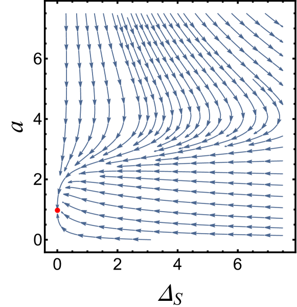
Figure 3: Flow diagram in the $\Delta_{S}-a$ plane with $g^{2}=g_{c}^{2}$ when the system contains only RSP. There is an stable fixed point(red point) $(g^{2},\Delta_{S}^{\ast},a^{\ast})=(g_{c}^{2},0,1)$. Within $g_{c}^{2}$ plane, no other fixed point exists and any RSP $\Delta_{S}$ is irrelevant at one-loop level. The system always flows into weak disorder regime.

Finite $g^{2}$ will always pull back the RG flow and RSP $\Delta_{S}$ is irrelevant eventually at one-loop level for any initial values. We find that SUSY is stable: an arbitrarily strong RSP flows to the weak coupling regime in the lowest energy limit. This means that the RSP is an irrelevant perturbation, which is consistent with the one-loop RG result in [82]. Previous results show that the RSP is marginally relevant for Dirac fermions, and will induce an instability of the system, leading to a diffusive motion of the Dirac fermions [42, 45, 56, 57, 52, 81, 54]. However, our result shows that, the RSP is rendered irrelevant by the critical fluctuations at the PDW QCP through the finite Yukawa coupling $g^{2}$ between fermion and boson. There exists no diffusive behaviors as long as $g^{2}$ is finite.

When more than one type of disorder exist, from the properties of the RG equation, Eqs. (12)-(14) that the coexistence of any two types disorder dynamically generate the third one. Thus we need to analyze the full set of RG equations given by Eqs. (8)-(13). It is easy to see that there is a fixed point given by $(v_{f},a^{*},g^{2\ast},\Delta_{S}^{\ast},\Delta_{M}^{\ast},\Delta_{V}^{\ast})=(v_{f},1,\frac{\epsilon}{3},0,0,0)$, where $v_{f}$ can take any values. Combining with the RG equation for coupling constants $u$ and $u_{+-}$, it turns out that this is the SUSY fixed point. Now we examine whether this fixed point is stable by expanding the RG equation at the fixed point, and calculate eigenvalues of the stability matrix (see Appendix C). The eigenvalues of the stability matrix are all negative except for one marginal direction at $v_{f}$. So we can conclude that the emergent SUSY is robust against weak disorders.

III (3+1)D Weyl semimetals

In this section, we examine the disorder effects on the emergent SUSY in (3+1)D WSMs [37]. The effective action of the disordered system in the vicinity of PDW QCP is given by

$$S = S_{f}+S_{b}+S_{I}+S_{\text{dis}},$$ (20)

$$S_{f} = \int d^{4}x\sum_{n=\pm}\Big{[}\psi_{n}^{\dagger}\partial_{\tau}\psi_{n}+\sum_{j=1}^{3}iv_{fj}\psi_{n}^{\dagger}\gamma_{n}^{j}\partial_{j}\psi_{n}\Big{]},\qquad$$ (21)

$$S_{b} = \int d^{4}x\bigg{\{}\sum_{n=\pm}\Big{[}|\partial_{\tau}\phi_{n}|^{2}+\sum_{j=1}^{3}v_{bj}^{2}|\partial_{j}\phi_{n}|^{2}$$

$$+r|\phi_{n}|^{2}+u|\phi_{n}|^{4}\Big{]}+u_{+-}|\phi_{+}|^{2}|\phi_{-}|^{2}\bigg{\}},$$

$$S_{I} = \int d^{4}xg\sum_{n=\pm}\Big{[}\phi_{n}\psi_{n}\sigma^{y}\psi_{n}+h.c.\Big{]},$$ (23)

$$S_{\text{dis}} = -\frac{1}{2}\int d^{3}xd\tau d\tau^{\prime}\Big{[}\Delta_{S}\big{(}\psi^{\dagger}_{\alpha}{\sigma}_{0}\psi_{\alpha}\big{)}_{x}\big{(}\psi^{\dagger}_{\beta}{\sigma}_{0}\psi_{\beta}\big{)}_{x^{\prime}}$$

$$+\sum_{i=x,y,z}\Delta_{i}\big{(}\psi^{\dagger}_{\alpha}{\sigma}_{i}\psi_{\alpha}\big{)}_{x}\big{(}\psi^{\dagger}_{\beta}{\sigma}_{i}\psi_{\beta}\big{)}_{x^{\prime}}\Big{]},$$

where $\gamma_{\pm}^{j}=({\sigma}^{x},{\sigma}^{y},\pm{\sigma}^{z})$. Now, $\psi_{\pm}$ denotes the two-component Weyl fermions at two Weyl points $\bm{Q}_{\pm}$, and $\phi_{\pm}$ is the superconducting order with momentum $2\bm{Q}_{\pm}$, respectively. In (3+1)D Weyl semimetal, RVP has three components, i.e., RM becomes the third component [83, 84]. In general, the fermion velocity is anisotropic, with unequal values along different directions. As shown in Ref. [37], even in the extremely anisotropic case, an emergent Lorentz symmetry can be established in the lowest energy limit. Our current concern is whether this emergent Lorentz symmetry can be broken by quenched disorder, thus it suffices to consider the isotopic case. We now can assume that $v_{fx}=v_{fy}=v_{fz}=v_{f}$, and also make the same assumption for the bosonic field. We employ the same symbol $a$ to identify the ratio between boson and fermion, and the same definition of $G_{0}$, $G_{1}$ and the rescaled couplings in Sec. II. Calculating the same diagrams in Fig. 2, we obtain the following RG equations:

$$\frac{d\ln v_{f}}{dl} = g^{2}(G_{1}-G_{0})-2\left(\Delta_{S}+\sum_{i}\Delta_{i}\right),$$ (25)

$$\frac{d\ln a^{2}}{dl} = \frac{g^{2}(1-a^{2})}{a^{2}}-2g^{2}(G_{1}-G_{0})+4\left(\Delta_{S}+\sum_{i}\Delta_{i}\right),$$ (26)

$$\frac{d\ln g^{2}}{dl} = \epsilon-g^{2}(3G_{1}-G_{0}+1)+\left(6\Delta_{S}+2\sum_{i}\Delta_{i}\right),$$ (27)

$$\frac{d\Delta_{S}}{dl} = (\epsilon-1)\Delta_{S}+2\Delta_{S}\left(\Delta_{S}+\sum_{i}\Delta_{i}\right)+\frac{2}{3}\sum_{i}\sum_{j\neq i}\Delta_{i}\Delta_{j}+g^{2}(G_{0}-3G_{2}-2G_{1})\Delta_{S},$$ (28)

$$\frac{d\Delta_{i}}{dl} = (\epsilon-1)\Delta_{i}+\frac{4}{3}\sum_{j\neq i}\Delta_{S}\Delta_{j}-\frac{2}{3}\Delta_{i}\left(\Delta_{S}+2\Delta_{i}-\sum_{j}\Delta_{j}\right)-\Delta_{i}g^{2}(G_{0}+G_{2}+2G_{1}),$$ (29)

in these equations, the index $i$ is summed over $x,y,z$. The analysis of these RG equations follows similarly as done in Sec. II. Firstly, we consider only a single vector component disorder exists, which means

$$\Delta_{i}\neq 0,\quad\Delta_{j\neq i}=0,\quad\Delta_{S}=0,$$ (30)

by substituting this conditions to Eqs. (25-29), three simplified RG equations for $a$, $g^{2}$ and $\Delta_{i}$ are obtained, we just exhibit the result for disorder coupling as

$$\frac{d\Delta_{i}}{dl} =(\epsilon-1)\Delta_{i}-\frac{2}{3}\Delta_{i}^{2}-\Delta_{i}g^{2}(G_{0}+G_{2}+2G_{1}).$$ (31)

Therefore, for an exact (3+1)D system corresponding to $\epsilon=0$, any component of RVP is irrelevant. As a result, in (3+1)D WSMs, the emergent SUSY is robust against any single component of RVP.

For there is only RSP in the system, we have $\Delta_{i}=0$. Now Eqs. (25) - (29) are simplified to

$$\frac{d\ln a^{2}}{dl}= \frac{g^{2}(1-a^{2})}{a^{2}}-2g^{2}(G_{1}-G_{0})+4\Delta_{S},$$ (32)

$$\frac{d\ln g^{2}}{dl}= \epsilon-g^{2}(3G_{1}-G_{0}+1)+6\Delta_{S},$$ (33)

$$\frac{d\Delta_{S}}{dl}= (\epsilon-1)\Delta_{S}+2\Delta_{S}^{2}$$

$$\qquad+g^{2}(G_{0}-3G_{2}-2G_{1})\Delta_{S},$$ (34)

according to Eq. (33), and noting the fact $3G_{1}-G_{0}+1>0$, the stable fixed point for $g^{2}$ is located at $g_{c}^{2}=6\Delta_{S}/(3G_{1}-G_{0}+1)$. Weak RSP itself is irrelevant as indicated in because $G_{0}-3G_{2}-2G_{1}<0$. Whereas for strong RSP, the scenario is similar to the case of (2+1) DSMs, namely, the RSP becomes irrelevant due to the interplay between the Weyl fermion and the PDW order parameter. We thus conclude that the the emergent SUSY is stable against RSP.

Next, we consider the coexisting case. According to Eq. (28), the coexistence of two components of RVP can dynamically generate RSP even when RSP does not exist at the beginning. We also learn from Eq. (29) that the coexistence of RSP and any component of RVP produce the other two components. Therefore, we need to consider the generic case in which all three components of RVP coexist with RSP. Now the disorder effects should be analyzed by solving the complete set of equations given by Eq. (25) - (29). It is hard to solve these coupled equations, but fortunately, it is simple to show that in the weak disorder regime the SUSY fixed point is stable against all random potentials, similar to the case of (2+1) DSMs.

IV Summary and discussion

In summary, we perform a standard perturbative RG to study the effect of disorder on the emergent SUSY in (2+1)D DSMs [37, 27] and (3+1)D WSMs [37]. According to our RG results, the effective SUSY fixed point is robust against any weak disorder irrespective of the type of disorder potentials. Our RG analysis of the disorder effects on the emergent SUSY appearing in (2+1)D DSMs [37, 27] and (3+1)D WSMs [37] can be directly extended to other analogous models, which may be more realistic to detect emergent SUSY in quantum materials. In our one-loop RG analysis, we have omitted new vertex that could be generated from the disorder potential and the Yukawa coupling. It will be interesting to include their effects although at tree-level they are irrelevant. Our work can shed new light on the understanding and exploring the emergent SUSY in realistic condensed matter systems.

Appendix A: Disorder potentials

In this section, we briefly consider the possible disorder potential in the two-component Dirac (Weyl) system. The original spinful fermion annihilation operator $\psi$ can be expand around two Dirac (Weyl) point $\bm{Q}_{\pm}$,

$$\psi(\bm{x})=e^{-i\bm{Q}_{+}\cdot\bm{x}}\psi_{+}(\bm{x})+e^{-i\bm{Q}_{-}\cdot\bm{x}}\psi_{-}(\bm{x}),$$ (35)

where $\psi_{\pm}$ corresponds to the two low-energy Dirac (Weyl) fermion. For the fermion system $\psi$, a general disorder potential takes the form,

$$H_{\mathrm{dis}}=\int d^{d}\bm{x}\psi^{\dagger}(\bm{x})\left(\sum_{\Gamma}V_{\Gamma}(\mathbf{x})\Gamma\right)\psi(\bm{x}),$$ (36)

where the $V_{\Gamma}(\mathbf{x})$ stands for the randomly distributed potential and $\Gamma=I,\sigma_{\mu}$ ($\mu=x,y,z$) labels type of the disorder potential. We focus on the quenched disorder potential $V_{\Gamma}(\mathbf{x})$, with Gaussian white noise potential characterized by the following identities:

$$\langle V_{\Gamma}(\mathbf{x})\rangle=0,\,\langle V_{\Gamma}(\mathbf{x})V_{\Gamma^{{}^{\prime}}}(\mathbf{x}^{\prime})\rangle=\Delta_{\Gamma}\delta_{\Gamma\Gamma^{{}^{\prime}}}\delta^{d}(\mathbf{x}-\mathbf{x}^{\prime}).$$ (37)

Substituting the fermion field Eq. (35) into the disordered Hamiltonian $H_{\text{dis}}$, we can arrive at the disorder Hamiltonian for the two low-energy Dirac (Weyl) fermion $\psi_{\pm}$. Notice that for the coupling between the two Dirac field, e.g. $\psi_{+}^{\dagger}(\bm{x})\Gamma\psi_{-}(\bm{x})$, there is an overall oscillating factor $e^{\pm i(\bm{Q}_{+}+\bm{Q}_{-})\cdot\bm{x}}$. Such disorder potential coupled the two Dirac (Weyl) fermion $\psi_{\pm}$ will be small in general. We only need to consider the disorder Hamiltonian Eq. (5) with respect to a piece of Dirac fermion. It should be emphasized that the two pieces of Dirac (Weyl) fermion share the same statistical distribution of random potential.

Appendix B: RG details

We present here the detailed calculation of Fig. 2(a)-Fig. 2(h) as well as the RG equations in $(2+1)$D, the calculation for $(3+1)$D is directly followed, which is not detailed shown here.

From the free action of fermions and bosons,

$$S_{f0} =\int d^{2}xd\tau\sum_{n=\pm}\psi_{n}^{\dagger}\Big{[}\partial_{\tau}+iv_{f}\sum_{j=1}^{2}\gamma_{j}\partial_{j}\Big{]}\psi_{n},$$ (38)

$$S_{b0} =\int d^{2}xd\tau\bigg{\{}\sum_{n=\pm}\Big{[}|\partial_{\tau}\phi_{n}|^{2}+v_{b}^{2}\sum_{j=1}^{2}|\partial_{j}\phi_{n}|^{2}\bigg{\}},$$ (39)

the free propagator for fermions and bosons are

$$G_{0}(k) =\frac{1}{ik_{\tau}-v_{f}\bm{\gamma}\cdot\mathbf{k}};$$

$$D_{0}(k) =\frac{1}{k_{\tau}^{2}+v_{b}^{2}\mathbf{k}^{2}}.$$

with $k=(k_{\tau},\bm{k})$ in the momentum space through replacement $(\partial_{\tau},\partial_{i})\rightarrow(ik_{\tau},ik_{i})$. The free propagators for the two pieces of Dirac fermion take the same form. For Fig. 2(a), it corresponds

$$\Pi(k) =-2g^{2}\int_{p}\text{Tr}\left[\sigma^{y}G_{0}^{T}(p)\sigma^{y}G_{0}(-p-k)\right]$$

$$=\frac{g^{2}S_{d}\Lambda^{-\epsilon}}{2(2\pi)^{d}v_{f}^{3}}l\Big{(}k_{\tau}^{2}+\Big{(}2-\frac{3}{d}\Big{)}v_{f}^{2}\bm{k}^{2}\Big{)}$$ (40)

where $\int_{p}\equiv\int dp_{\tau}d^{d}\bm{p}/(2\pi)^{D}$ is the $D=d+1$ dimensional momentum integral and $S_{d}=2\pi^{d/2}/\Gamma(d/2)$ is the area of the unit sphere in $d$ dimensions. For Fig. 2(c), it gives

$$\Sigma_{f}^{(b)}(k)=-4g^{2}(-)\int_{p}\sigma^{y}G_{0}^{T}(p)\sigma^{y}D_{0}(-k-p)$$

$$=\frac{g^{2}S_{d}\Lambda^{-\epsilon}}{2(2\pi)^{d}v_{f}^{3}}l\Big{(}\frac{4(ik_{\tau})}{a(a+1)^{2}}-\frac{4(2a+1)}{ad(a+1)^{2}}(v_{f}\bm{\gamma}\cdot\mathbf{k})\Big{)}$$

$$=\frac{g^{2}S_{d}\Lambda^{-\epsilon}}{2(2\pi)^{d}v_{f}^{3}}l\Big{(}G_{0}(ik_{\tau})-G_{1}(v_{f}\bm{\gamma}\cdot\mathbf{k})\Big{)}$$ (41)

The diagram of Fig. 2(d) is ,

$$\Sigma_{f}^{(c)}(k) =-\sum_{\Gamma}(\Delta_{\Gamma}+\Delta_{\Gamma}^{\prime})\int\frac{d^{d}\mathbf{k}}{(2\pi)^{d}}\Gamma G_{0}(k)\Gamma$$

$$=\sum_{\Gamma}(\Delta_{\Gamma}+\Delta_{\Gamma}^{\prime})\frac{\Lambda^{1-\epsilon}S_{d}}{(2\pi)^{d}v_{f}^{2}}(ik_{\tau})\ell,$$ (42)

which only contribute to the velocity renormalization at one-loop. The diagram of Fig. 2(e) is given by

$$\delta\Delta_{\Gamma}^{(d)}= -8\Delta_{\Gamma}{g}^{2}\int_{k}\sigma^{y}D(-k)G^{T}(k)\Gamma^{T}G^{T}(k)\sigma^{y}$$ (43)

$$\delta\Delta_{\Gamma}^{\prime(d)}= -8\Delta_{\Gamma}^{\prime}{g}^{2}\int_{k}\sigma^{y}D(-k)G^{T}(k)\Gamma^{T}G^{T}(k)\sigma^{y}$$ (44)

Calculating out these integrals for different $\Gamma_{a}$ one by one, we have

$$\delta\Delta_{S}^{(d)}= \Delta_{S}\frac{g^{2}S_{d}\Lambda^{-\epsilon}}{2(2\pi)^{d}v_{f}^{3}}(G_{0}-dG_{2}),$$ (45)

$$\delta\Delta_{M}^{(d)}= \Delta_{M}\frac{g^{2}S_{d}\Lambda^{-\epsilon}}{2(2\pi)^{d}v_{f}^{3}}(-G_{0}-dG_{2}),$$ (46)

$$\delta\Delta_{V}^{(d)}= \Delta_{V}\frac{g^{2}S_{d}\Lambda^{-\epsilon}}{2(2\pi)^{d}v_{f}^{3}}(-G_{0}),$$ (47)

and same for $\Delta\rightarrow\Delta^{\prime}$. The diagram of Fig. 2(b) involves $\Delta_{\gamma}$-vertex and is given by

$$\delta g^{(h)}=g\sum_{\Gamma}\Delta_{\Gamma}\int_{\bm{k}}\Gamma^{T}G_{+}^{T}(k)\sigma^{y}G_{+}(-k)\Gamma$$

$$= gl\sum_{\Gamma}\frac{\Delta_{\Gamma}\Lambda^{1-\epsilon}S_{d}}{(2\pi)^{d}v_{f}^{2}}\Gamma^{T}\sigma^{y}\Gamma$$ (48)

The remaining diagrams Fig. 2(f,g,h) correspond to pure coupling between disorder potentials [67], which can be obtained as follows,

$$\delta\Delta_{S}^{(e,f,g)}= \Big{(}\frac{S_{d}}{(2\pi)^{d}v_{f}^{2}\Lambda^{2-d}}\Big{)}l\Big{[}+2\Delta_{S}\big{(}\Delta_{S}+\Delta_{M}+2\Delta_{V}\big{)}+4\Delta_{M}\Delta_{V}\Big{]}$$ (49)

$$\delta\Delta_{M}^{(e,f,g)}= \Big{(}\frac{S_{d}}{(2\pi)^{d}v_{f}^{2}\Lambda^{2-d}}\Big{)}l\Big{[}-2\Delta_{M}\big{(}\Delta_{S}+\Delta_{M}-2\Delta_{V}\big{)}+4\Delta_{S}\Delta_{V}\Big{]}$$ (50)

$$\delta\Delta_{V}^{(e,f,g)}= \Big{(}\frac{S_{d}}{(2\pi)^{d}v_{f}^{2}\Lambda^{2-d}}\Big{)}l\Big{[}2\Delta_{M}\Delta_{S}\Big{]}$$ (51)

and similarly for the other three terms,

$$\delta\Delta_{S}^{\prime(e,f,g)}= \Big{(}\frac{S_{d}}{(2\pi)^{d}v_{f}^{2}\Lambda^{2-d}}\Big{)}l\Big{[}+2\Delta_{S}^{\prime}\big{(}\Delta_{S}+\Delta_{M}+2\Delta_{V}\big{)}+4\Delta_{M}^{\prime}\Delta_{V}^{\prime}\Big{]}$$ (52)

$$\delta\Delta_{M}^{\prime(e,f,g)}= \Big{(}\frac{S_{d}}{(2\pi)^{d}v_{f}^{2}\Lambda^{2-d}}\Big{)}l\Big{[}-2\Delta_{M}^{\prime}\big{(}\Delta_{S}+\Delta_{M}-2\Delta_{V}\big{)}+4\Delta_{S}^{\prime}\Delta_{V}^{\prime}\Big{]}$$ (53)

$$\delta\Delta_{V}^{\prime(e,f,g)}= \Big{(}\frac{S_{d}}{(2\pi)^{d}v_{f}^{2}\Lambda^{2-d}}\Big{)}l\Big{[}2\Delta_{M}^{\prime}\Delta_{S}^{\prime}\Big{]}$$ (54)

According to above results, label and rescale the couplings as follows:

$$G_{0}=\frac{4}{a(1+a)^{2}},\quad G_{1}=\frac{4(1+2a)}{da(1+a)^{2}},\quad G_{2}=\frac{4(2+a)}{da(1+a)^{2}},\quad\frac{g^{2}\Lambda^{-\epsilon}S_{d}}{2(2\pi)^{d}v_{f}^{3}}\rightarrow g^{2},\quad\frac{\Delta_{\Gamma}\Lambda^{1-\epsilon}S_{d}}{(2\pi)^{d}v_{f}^{2}}\rightarrow\Delta_{\Gamma}.$$ (55)

Then, the results obtained for Fig. 2(a)-Fig. 2(h) can be simplified, leading to the one-loop quantum corrections of the action. These one-loop results produce the RG equations

$$\frac{dv_{f}}{dl} =v_{f}\Big{[}g^{2}(G_{1}-G_{0})-\sum_{\Gamma}\Delta_{\Gamma}-\sum_{\Gamma}\Delta_{\Gamma}^{\prime}\Big{]},$$ (56)

$$\frac{da}{dl} =g^{2}\Big{(}\frac{1-a^{2}}{2a}+a(G_{0}-G_{1})\Big{)}+a\sum_{\Gamma}\Delta_{\Gamma}+a\sum_{\Gamma}\Delta_{\Gamma}^{\prime},$$ (57)

$$\frac{dg^{2}}{dl} =\epsilon g^{2}-g^{4}\big{(}1-G_{0}+3G_{1}\big{)}+\big{(}4\Delta_{S}-\sum_{\Gamma}\Delta_{\Gamma}+3\sum_{\Gamma}{\Delta}_{\Gamma}^{\prime}\big{)}g^{2},$$ (58)

$$\frac{d\Delta_{S}}{dl} =\big{(}\epsilon-1\big{)}\Delta_{S}+2\Delta_{S}\big{(}\Delta_{S}+\Delta_{M}+2\Delta_{V}\big{)}+4\Delta_{M}\Delta_{V}+(G_{0}-3G_{2}-2G_{1})\Delta_{S}g^{2},$$ (59)

$$\frac{d\Delta_{M}}{dl} =\big{(}\epsilon-1\big{)}\Delta_{M}-2\Delta_{M}\big{(}\Delta_{S}+\Delta_{M}-2\Delta_{V}\big{)}+4\Delta_{S}\Delta_{V}-(G_{0}+3G_{2}+2G_{1})\Delta_{M}g^{2},$$ (60)

$$\frac{d\Delta_{V}}{dl} =\big{(}\epsilon-1\big{)}\Delta_{V}+2\Delta_{M}\Delta_{S}-(G_{0}+2G_{1})\Delta_{V}g^{2},$$ (61)

$$\frac{d\Delta_{S}^{\prime}}{dl} =\big{(}\epsilon-1\big{)}\Delta_{S}^{\prime}+2\Delta_{S}^{\prime}\big{(}\Delta_{S}+\Delta_{M}+2\Delta_{V}\big{)}+4\Delta_{M}^{\prime}\Delta_{V}^{\prime}+(G_{0}-3G_{2}-2G_{1})\Delta_{S}^{\prime}g^{2},$$ (62)

$$\frac{d\Delta_{M}^{\prime}}{dl} =\big{(}\epsilon-1\big{)}\Delta_{M}^{\prime}-2\Delta_{M}^{\prime}\big{(}\Delta_{S}+\Delta_{M}-2\Delta_{V}\big{)}+4\Delta_{S}^{\prime}\Delta_{V}^{\prime}-(G_{0}+3G_{2}+2G_{1})\Delta_{M}^{\prime}g^{2},$$ (63)

$$\frac{d\Delta_{V}^{\prime}}{dl} =\big{(}\epsilon-1\big{)}\Delta_{V}^{\prime}+2\Delta_{M}^{\prime}\Delta_{S}^{\prime}-(G_{0}+2G_{1})\Delta_{V}^{\prime}g^{2},$$ (64)

Since the initial values of the parameters are $\Delta_{\Gamma}^{0}=\Delta_{\Gamma}^{\prime 0}$, $\Delta_{\Gamma}$ and $\Delta_{\Gamma}^{\prime}$ will flow in the same way. We can simplify the equations by taken $\Delta_{\Gamma}^{\prime}=\Delta_{\Gamma}$ and produce the Eqs. (8) - (13).

For the case of $(3+1)D$, due to the change of disorder typies, the one-loop corrections of disorder couplings need to recalculate, the extension is direct for which we do not show details here.

Appendix C: general disorder case

In this section, we study the case where all the disorder potential is appeared. We focus on the regime near the Lorentz symmetric fixed point, $a=1+\delta a$ with small $\delta a\ll 1$. The RG equations in 2D now become,

$$\frac{dv_{f}}{dl} = v_{f}\Big{[}g^{2}\frac{2}{3}\delta a-2\sum_{\Gamma}\Delta_{\mu}\Big{]},$$ (65)

$$\frac{d\delta a}{dl} = \Big{(}-\frac{5}{3}g^{2}+2\sum_{\Gamma}\Delta_{\Gamma}\Big{)}\delta a,$$ (66)

$$\frac{dg^{2}}{dl} = \epsilon g^{2}-g^{4}\big{(}3-2\delta a\big{)}+\big{(}4\Delta_{S}+2\sum_{\Gamma}\Delta_{\Gamma}\big{)}g^{2},$$ (67)

$$\frac{d\Delta_{S}}{dl} = \big{(}\epsilon-1\big{)}\Delta_{S}+2\Delta_{S}\big{(}\Delta_{S}+\Delta_{M}+2\Delta_{V}\big{)}+4\Delta_{M}\Delta_{V}+(-4+\frac{17}{3}\delta a)\Delta_{S}g^{2},$$ (68)

$$\frac{d\Delta_{M}}{dl} = \big{(}\epsilon-1\big{)}\Delta_{M}-2\Delta_{M}\big{(}\Delta_{S}+\Delta_{M}-2\Delta_{V}\big{)}+4\Delta_{S}\Delta_{V}-(6-\frac{29}{3}\delta a)\Delta_{M}g^{2},$$ (69)

$$\frac{d\Delta_{V}}{dl} = \big{(}\epsilon-1\big{)}\Delta_{V}+2\Delta_{M}\Delta_{S}-(3-\frac{14}{3}\delta a)\Delta_{V}g^{2},$$ (70)

There is a fixed point given by $(v_{f},a^{*},g^{2\ast},\Delta_{S}^{\ast},\Delta_{M}^{\ast},\Delta_{V}^{\ast})=(v_{f},1,\frac{\epsilon}{3},0,0,0)$. For small disorder case, the stability matrix at this fixed point is

$$\left(\begin{array}[]{cccccc}0&\frac{2}{9}\epsilon v_{f}&0&-2v_{f}&-2v_{f}&-2v_{f}\\ 0&-\frac{5}{9}\epsilon&0&2&2&2\\ 0&\frac{2}{9}\epsilon^{2}&-\epsilon&2\epsilon&\frac{2}{3}\epsilon&\frac{2}{3}\epsilon\\ 0&0&0&-1-\frac{\epsilon}{3}&0&0\\ 0&0&0&0&-1-\epsilon&0\\ 0&0&0&0&0&-1\end{array}\right).$$ (77)

The eigenvalues of the stability matrix are all negative except for one marginal direction at $v_{f}$. We can conclude that the coupling between Yukawa potential and disorder will suppress weak random disorder potential. Similarly argument can also be applied to three dimensional case.

References

- Weinberg [2000] S. Weinberg, The quantum theory of fields, Vol. 3 (Cambridge university press, 2000).
- Gervais and Sakita [1971] J.-L. Gervais and B. Sakita, Field theory interpretation of supergauges in dual models, Nuclear Physics B 34, 632 (1971).
- Wess and Zumino [1974] J. Wess and B. Zumino, Supergauge transformations in four dimensions, Nuclear Physics B 70, 39 (1974).
- Dimopoulos and Georgi [1981] S. Dimopoulos and H. Georgi, Softly broken supersymmetry and su(5), Nuclear Physics B 193, 150 (1981).
- Cremmer et al. [1983] E. Cremmer, S. Ferrara, C. Kounnas, and D. Nanopoulos, Naturally vanishing cosmological constant in n=1 supergravity, Physics Letters B 133, 61 (1983).
- Seiberg and Witten [1994] N. Seiberg and E. Witten, Electric-magnetic duality, monopole condensation, and confinement in n=2 supersymmetric yang-mills theory, Nuclear Physics B 426, 19 (1994).
- Seiberg [1995] N. Seiberg, Electric-magnetic duality in supersymmetric non-abelian gauge theories, Nuclear Physics B 435, 129 (1995).
- Wan et al. [2011] X. Wan, A. M. Turner, A. Vishwanath, and S. Y. Savrasov, Topological semimetal and fermi-arc surface states in the electronic structure of pyrochlore iridates, Phys. Rev. B 83, 205101 (2011).
- Xu et al. [2011] G. Xu, H. Weng, Z. Wang, X. Dai, and Z. Fang, Chern semimetal and the quantized anomalous hall effect in , Phys. Rev. Lett. 107, 186806 (2011).
- Burkov and Balents [2011] A. A. Burkov and L. Balents, Weyl semimetal in a topological insulator multilayer, Phys. Rev. Lett. 107, 127205 (2011).
- Weng et al. [2015] H. Weng, C. Fang, Z. Fang, B. A. Bernevig, and X. Dai, Weyl semimetal phase in noncentrosymmetric transition-metal monophosphides, Phys. Rev. X 5, 011029 (2015).
- Huang et al. [2015] S.-M. Huang, S.-Y. Xu, I. Belopolski, C.-C. Lee, G. Chang, B. Wang, N. Alidoust, G. Bian, M. Neupane, C. Zhang, et al., A weyl fermion semimetal with surface fermi arcs in the transition metal monopnictide taas class, Nature communications 6, 1 (2015).
- Xu et al. [2015] S.-Y. Xu, I. Belopolski, N. Alidoust, M. Neupane, G. Bian, C. Zhang, R. Sankar, G. Chang, Z. Yuan, C.-C. Lee, et al., Discovery of a weyl fermion semimetal and topological fermi arcs, Science 349, 613 (2015).
- Lv et al. [2015] B. Q. Lv, H. M. Weng, B. B. Fu, X. P. Wang, H. Miao, J. Ma, P. Richard, X. C. Huang, L. X. Zhao, G. F. Chen, Z. Fang, X. Dai, T. Qian, and H. Ding, Experimental discovery of weyl semimetal taas, Phys. Rev. X 5, 031013 (2015).
- Yang et al. [2015] L. Yang, Z. Liu, Y. Sun, H. Peng, H. Yang, T. Zhang, B. Zhou, Y. Zhang, Y. Guo, M. Rahn, et al., Weyl semimetal phase in the non-centrosymmetric compound taas, Nature physics 11, 728 (2015).
- Curci and Veneziano [1987] G. Curci and G. Veneziano, Supersymmetry and the lattice: A reconciliation?, Nuclear Physics B 292, 555 (1987).
- Goh et al. [2005] H.-S. Goh, M. A. Luty, and S.-P. Ng, Supersymmetry without supersymmetry, Journal of High Energy Physics 2005, 040 (2005).
- [18] S. Thomas, Emergent supersymmetry, kitp talk, 2005.
- Prakash and Wang [2021a] A. Prakash and J. Wang, Boundary supersymmetry of fermionic symmetry-protected topological phases, Phys. Rev. Lett. 126, 236802 (2021a).
- Prakash and Wang [2021b] A. Prakash and J. Wang, Unwinding fermionic symmetry-protected topological phases: Supersymmetry extension, Phys. Rev. B 103, 085130 (2021b).
- Turzillo and You [2021] A. Turzillo and M. You, Supersymmetric boundaries of one-dimensional phases of fermions beyond symmetry-protected topological states, Phys. Rev. Lett. 127, 026402 (2021).
- Li et al. [2018] Z.-X. Li, A. Vaezi, C. B. Mendl, and H. Yao, Numerical observation of emergent spacetime supersymmetry at quantum criticality, Science advances 4, eaau1463 (2018).
- Li and Yao [2017] Z.-X. Li and H. Yao, Edge stability and edge quantum criticality in two-dimensional interacting topological insulators, Phys. Rev. B 96, 241101 (2017).
- Li et al. [2016] Z.-X. Li, Y.-F. Jiang, and H. Yao, Majorana-time-reversal symmetries: A fundamental principle for sign-problem-free quantum monte carlo simulations, Phys. Rev. Lett. 117, 267002 (2016).
- Jian et al. [2017] S.-K. Jian, C.-H. Lin, J. Maciejko, and H. Yao, Emergence of supersymmetric quantum electrodynamics, Phys. Rev. Lett. 118, 166802 (2017).
- Yu et al. [2019] J. Yu, R. Roiban, S.-K. Jian, and C.-X. Liu, Finite-scale emergence of supersymmetry at first-order quantum phase transition, Phys. Rev. B 100, 075153 (2019).
- Lee [2007] S.-S. Lee, Emergence of supersymmetry at a critical point of a lattice model, Phys. Rev. B 76, 075103 (2007).
- Yu and Yang [2010] Y. Yu and K. Yang, Simulating the wess-zumino supersymmetry model in optical lattices, Phys. Rev. Lett. 105, 150605 (2010).
- Hasan and Kane [2010] M. Z. Hasan and C. L. Kane, Colloquium: Topological insulators, Rev. Mod. Phys. 82, 3045 (2010).
- Qi and Zhang [2011] X.-L. Qi and S.-C. Zhang, Topological insulators and superconductors, Rev. Mod. Phys. 83, 1057 (2011).
- Grover et al. [2014] T. Grover, D. Sheng, and A. Vishwanath, Emergent space-time supersymmetry at the boundary of a topological phase, Science 344, 280 (2014).
- Ponte and Lee [2014] P. Ponte and S.-S. Lee, Emergence of supersymmetry on the surface of three-dimensional topological insulators, New Journal of Physics 16, 013044 (2014).
- Zerf et al. [2016] N. Zerf, C.-H. Lin, and J. Maciejko, Superconducting quantum criticality of topological surface states at three loops, Phys. Rev. B 94, 205106 (2016).
- Friedan et al. [1984] D. Friedan, Z. Qiu, and S. Shenker, Conformal invariance, unitarity, and critical exponents in two dimensions, Phys. Rev. Lett. 52, 1575 (1984).
- Foda [1988] O. Foda, A supersymmetric phase transition in josephson-tunnel-junction arrays, Nuclear Physics B 300, 611 (1988).
- Huijse et al. [2015] L. Huijse, B. Bauer, and E. Berg, Emergent supersymmetry at the ising–berezinskii-kosterlitz-thouless multicritical point, Phys. Rev. Lett. 114, 090404 (2015).
- Jian et al. [2015] S.-K. Jian, Y.-F. Jiang, and H. Yao, Emergent spacetime supersymmetry in 3d weyl semimetals and 2d dirac semimetals, Phys. Rev. Lett. 114, 237001 (2015).
- Ruan et al. [2016a] J. Ruan, S.-K. Jian, H. Yao, H. Zhang, S.-C. Zhang, and D. Xing, Symmetry-protected ideal weyl semimetal in hgte-class materials, Nature communications 7, 1 (2016a).
- Ruan et al. [2016b] J. Ruan, S.-K. Jian, D. Zhang, H. Yao, H. Zhang, S.-C. Zhang, and D. Xing, Ideal weyl semimetals in the chalcopyrites , , , and , Phys. Rev. Lett. 116, 226801 (2016b).
- Lee and Ramakrishnan [1985] P. A. Lee and T. V. Ramakrishnan, Disordered electronic systems, Rev. Mod. Phys. 57, 287 (1985).
- Altshuler and Aronov [1985] B. Altshuler and A. G. Aronov, Electron-electron interactions in disordered systems ed al efros and m pollak, Amsterdam: North-Holland) p 1, 155 (1985).
- Fradkin [1986] E. Fradkin, Critical behavior of disordered degenerate semiconductors. ii. spectrum and transport properties in mean-field theory, Phys. Rev. B 33, 3263 (1986).
- Belitz and Kirkpatrick [1994] D. Belitz and T. R. Kirkpatrick, The anderson-mott transition, Rev. Mod. Phys. 66, 261 (1994).
- Abrahams et al. [2001] E. Abrahams, S. V. Kravchenko, and M. P. Sarachik, Metallic behavior and related phenomena in two dimensions, Rev. Mod. Phys. 73, 251 (2001).
- Altland et al. [2002] A. Altland, B. Simons, and M. Zirnbauer, Theories of low-energy quasi-particle states in disordered d-wave superconductors, Physics Reports 359, 283 (2002).
- Das Sarma et al. [2011] S. Das Sarma, S. Adam, E. H. Hwang, and E. Rossi, Electronic transport in two-dimensional graphene, Rev. Mod. Phys. 83, 407 (2011).
- Kotov et al. [2012] V. N. Kotov, B. Uchoa, V. M. Pereira, F. Guinea, and A. H. Castro Neto, Electron-electron interactions in graphene: Current status and perspectives, Rev. Mod. Phys. 84, 1067 (2012).
- Yerzhakov and Maciejko [2018] H. Yerzhakov and J. Maciejko, Disordered fermionic quantum critical points, Phys. Rev. B 98, 195142 (2018).
- Stauber et al. [2005] T. Stauber, F. Guinea, and M. A. H. Vozmediano, Disorder and interaction effects in two-dimensional graphene sheets, Phys. Rev. B 71, 041406 (2005).
- Herbut et al. [2008] I. F. Herbut, V. Juričić, and O. Vafek, Coulomb interaction, ripples, and the minimal conductivity of graphene, Phys. Rev. Lett. 100, 046403 (2008).
- Vafek and Case [2008] O. Vafek and M. J. Case, Renormalization group approach to two-dimensional coulomb interacting dirac fermions with random gauge potential, Phys. Rev. B 77, 033410 (2008).
- Goswami and Chakravarty [2011] P. Goswami and S. Chakravarty, Quantum criticality between topological and band insulators in dimensions, Phys. Rev. Lett. 107, 196803 (2011).
- Wang and Liu [2014] J.-R. Wang and G.-Z. Liu, Influence of coulomb interaction on the anisotropic dirac cone in graphene, Phys. Rev. B 89, 195404 (2014).
- Roy and Das Sarma [2014] B. Roy and S. Das Sarma, Diffusive quantum criticality in three-dimensional disordered dirac semimetals, Phys. Rev. B 90, 241112 (2014).
- Zhao et al. [2016] P.-L. Zhao, J.-R. Wang, A.-M. Wang, and G.-Z. Liu, Interplay of coulomb interaction and disorder in a two-dimensional semi-dirac fermion system, Phys. Rev. B 94, 195114 (2016).
- Ostrovsky et al. [2006] P. M. Ostrovsky, I. V. Gornyi, and A. D. Mirlin, Electron transport in disordered graphene, Phys. Rev. B 74, 235443 (2006).
- Foster and Aleiner [2008] M. S. Foster and I. L. Aleiner, Graphene via large : A renormalization group study, Phys. Rev. B 77, 195413 (2008).
- Yerzhakov and Maciejko [2021] H. Yerzhakov and J. Maciejko, Random-mass disorder in the critical gross-neveu-yukawa models, Nuclear Physics B 962, 115241 (2021).
- Roy et al. [2016] B. Roy, V. Juričić, and S. Das Sarma, Universal optical conductivity of a disordered weyl semimetal, Scientific reports 6, 1 (2016).
- Kim et al. [1997] D. H. Kim, P. A. Lee, and X.-G. Wen, Massless dirac fermions, gauge fields, and underdoped cuprates, Phys. Rev. Lett. 79, 2109 (1997).
- Lee et al. [2006] P. A. Lee, N. Nagaosa, and X.-G. Wen, Doping a mott insulator: Physics of high-temperature superconductivity, Rev. Mod. Phys. 78, 17 (2006).
- Wang [2013] J. Wang, Velocity renormalization of nodal quasiparticles in -wave superconductors, Phys. Rev. B 87, 054511 (2013).
- Wang et al. [2011] J. Wang, G.-Z. Liu, and H. Kleinert, Disorder effects at a nematic quantum critical point in -wave cuprate superconductors, Phys. Rev. B 83, 214503 (2011).
- Furneaux et al. [1995] J. E. Furneaux, S. V. Kravchenko, W. E. Mason, G. E. Bowker, and V. M. Pudalov, Destruction of the quantum hall effect with increasing disorder, Phys. Rev. B 51, 17227 (1995).
- Ye and Sachdev [1998] J. Ye and S. Sachdev, Coulomb interactions at quantum hall critical points of systems in a periodic potential, Phys. Rev. Lett. 80, 5409 (1998).
- Ye [1999] J. Ye, Effects of weak disorders on quantum hall critical points, Phys. Rev. B 60, 8290 (1999).
- Ludwig et al. [1994] A. W. W. Ludwig, M. P. A. Fisher, R. Shankar, and G. Grinstein, Integer quantum hall transition: An alternative approach and exact results, Phys. Rev. B 50, 7526 (1994).
- Zhao et al. [2017] P.-L. Zhao, A.-M. Wang, and G.-Z. Liu, Effects of random potentials in three-dimensional quantum electrodynamics, Phys. Rev. B 95, 235144 (2017).
- González et al. [1993] J. González, F. Guinea, and M. Vozmediano, The electronic spectrum of fullerenes from the dirac equation, Nuclear Physics B 406, 771 (1993).
- González et al. [1994] J. González, F. Guinea, and M. Vozmediano, Non-fermi liquid behavior of electrons in the half-filled honeycomb lattice (a renormalization group approach), Nuclear Physics B 424, 595 (1994).
- Nersesyan et al. [1995] A. Nersesyan, A. Tsvelik, and F. Wenger, Disorder effects in two-dimensional fermi systems with conical spectrum: exact results for the density of states, Nuclear Physics B 438, 561 (1995).
- Castro Neto et al. [2009] A. H. Castro Neto, F. Guinea, N. M. R. Peres, K. S. Novoselov, and A. K. Geim, The electronic properties of graphene, Rev. Mod. Phys. 81, 109 (2009).
- Peres [2010] N. M. R. Peres, Colloquium: The transport properties of graphene: An introduction, Rev. Mod. Phys. 82, 2673 (2010).
- Mucciolo and Lewenkopf [2010] E. R. Mucciolo and C. H. Lewenkopf, Disorder and electronic transport in graphene, Journal of Physics: Condensed Matter 22, 273201 (2010).
- Meyer et al. [2007] J. C. Meyer, A. K. Geim, M. I. Katsnelson, K. S. Novoselov, T. J. Booth, and S. Roth, The structure of suspended graphene sheets, Nature 446, 60 (2007).
- Champel and Florens [2010] T. Champel and S. Florens, High magnetic field theory for the local density of states in graphene with smooth arbitrary potential landscapes, Phys. Rev. B 82, 045421 (2010).
- Viola Kusminskiy et al. [2011] S. Viola Kusminskiy, D. K. Campbell, A. H. Castro Neto, and F. Guinea, Pinning of a two-dimensional membrane on top of a patterned substrate: The case of graphene, Phys. Rev. B 83, 165405 (2011).
- Lerner [2003] I. V. Lerner, Nonlinear sigma model for normal and superconducting systems: A pedestrian approach (2003).
- Roy and Das Sarma [2016] B. Roy and S. Das Sarma, Quantum phases of interacting electrons in three-dimensional dirty dirac semimetals, Phys. Rev. B 94, 115137 (2016).
- Shankar [1994] R. Shankar, Renormalization-group approach to interacting fermions, Rev. Mod. Phys. 66, 129 (1994).
- Foster [2012] M. S. Foster, Multifractal nature of the surface local density of states in three-dimensional topological insulators with magnetic and nonmagnetic disorder, Phys. Rev. B 85, 085122 (2012).
- Nandkishore et al. [2013] R. Nandkishore, J. Maciejko, D. A. Huse, and S. L. Sondhi, Superconductivity of disordered dirac fermions, Phys. Rev. B 87, 174511 (2013).
- Sbierski et al. [2016] B. Sbierski, K. S. C. Decker, and P. W. Brouwer, Weyl node with random vector potential, Phys. Rev. B 94, 220202 (2016).
- Syzranov and Radzihovsky [2018] S. V. Syzranov and L. Radzihovsky, High-dimensional disorder-driven phenomena in weyl semimetals, semiconductors, and related systems, Annual Review of Condensed Matter Physics 9, 35 (2018).