Electroweak Phase Transition and Gravitational Waves in the Type-II Seesaw Model

Abstract

The type-II seesaw model is a possible candidate for simultaneously explaining non-vanishing neutrino masses and the observed baryon asymmetry of the Universe. In this work, we study in detail the pattern of phase transition and the gravitational wave production of this model. We find a strong first-order electroweak phase transition generically prefers positive Higgs portal couplings and a light triplet below $\sim 550$ GeV. In addition, we find the gravitational wave yield generated during the phase transition would be at the edge of BBO sensitivity and could be further examined by Ultimate-DECIGO.

1 Introduction

The discovery of the Higgs boson in 2012 ATLAS:2012yve ; CMS:2012qbp completes the picture of the Standard Model (SM). However, within the SM framework, it is recognized that neutrinos are exactly massless particles as a result of a global U(1)_ℓ symmetry, conflicting with the observed phenomena of neutrino oscillations Fukuda:1998mi ; Ahmad:2001an . Furthermore, the phase transition with the observed 125 GeV Higgs boson in the SM will be of a crossover type Kajantie:1995kf ; Kajantie:1996mn ; Kajantie:1996qd , thus making the SM inadequate to explain the observed asymmetry of baryons Planck:2018vyg . Both these facts, together with some other fundamental questions like the nature of dark matter, imply that the SM cannot be the complete theory and extension of it is needed.

Among those extensions of the SM that can be responsible for massive neutrinos, the type-I, -II and -III seesaw models Minkowski:1977sc ; Ramond:1979py ; GellMann:1980vs ; Yanagida:1979as ; Mohapatra:1979ia ; Schechter:1980gr ; Schechter:1981cv ; Konetschny:1977bn ; Cheng:1980qt ; Lazarides:1980nt ; Magg:1980ut ; Foot:1988aq ; Witten:1985bz ; Mohapatra:1986aw ; Mohapatra:1986bd ; Val86 ; Barr:2003nn ; Mohapatra:1980yp , inspired by the pioneering work of Weinberg Weinberg:1979sa , have been extensively studied as they can naturally induce neutrino masses through the seesaw mechanism. In particular, all these three models predict the violation of lepton numbers by two units in contrast to their conservation in the SM. While it is not yet clear which mechanism is realized in practice, nowadays it is widely known that the type-I and -III models would be well beyond the reach of current experiments due to the largeness of the seesaw scales. In contrast, allowing the neutrino Yukawa couplings to be tiny, low-scale type-I and -III seesaw models would become possible and have also been investigated in literatures Han:2006ip ; Atre:2009rg ; FileviezPerez:2009hdc ; Alva:2014gxa ; Cai:2017mow ; Dev:2018sel .

We focus on the type-II seesaw model in this work, which is obtained by extending the SM Higgs sector with a complex triplet that transforms as (1,3,2) under the SM gauge group. The type-II seesaw model differents from the other two seesaw models in that it allows large neutrino Yukawa couplings simultaneously with a light seesaw scale even below TeV. This can be realized with a small triplet vacuum expectation value that naturally generates tiny neutrino masses with even $\mathcal{O}(1)$ neutrino Yukawa couplings Du:2018eaw . In addition, since the complex scalar transforms as a triplet under $\rm SU(2)_{L}$, new interactions between the SM Higgs doublet and the complex triplet will present and modify the Higgs potential. The modified Higgs potential could then change the phase transition type of the SM, thus also serve as a possible candidate for explaining the observed baryon asymmetry of the Universe Planck:2018vyg . While this model have been intensively studied experimentally OPAL:1992glr ; OPAL:2001luy ; Aaltonen:2011rta ; Aad:2012cg ; ATLAS:2012mn ; ATLAS:2012hi ; Aad:2014hja ; ATLAS:2014kca ; Aad:2015oga ; Sirunyan:2017ret ; Aaboud:2017qph and theoretically Machacek:1983tz ; Machacek:1983fi ; Machacek:1984zw ; Arason:1991ic ; Ford:1992pn ; Barger:1992ac ; Luo:2002ey ; Chao:2006ye ; Schmidt:2007nq ; Dey:2008jm ; Arhrib:2011uy ; Chao:2012mx ; Chun:2012jw ; Bonilla:2015eha ; Haba:2016zbu ; Cai:2017mow ; Li:2018jns ; Agrawal:2018pci ; Du:2018eaw at colliders, the pattern of its phase transition in this model have not yet been investigated to the best of our knowledge.

As mentioned in last paragraph, the modified Higgs potential, due to new interactions between the doublet and the triplet, could change the phase transition of the SM Higgs from a crossover type to a strong first-order phase transition. The strong first-order phase transition is a necessary condition that validates the departure from thermal equilibrium, one of the three Sakharov’s conditions Sakharov:1967dj . As a result, the triplet would be possible to explain the dynamic generation of the baryon asymmetry of the Universe through the electroweak baryogenesis paradigm Kuzmin:1985mm ; Cohen:1990it ; Cohen:1993nk ; Quiros:1994dr ; Rubakov:1996vz ; Funakubo:1996dw ; Trodden:1998ym ; Bernreuther:2002uj ; Morrissey:2012db ; DiBari:2013rga . On the other hand, stochastic background of gravitational waves could also be generated during the first-order phase transition. And recently, the observation of gravitational waves from LIGO and VIRGO has opened a new window to probe new physics beyond the SM LIGOScientific:2016aoc ; LIGOScientific:2017vwq ; LIGOScientific:2018mvr ; LIGOScientific:2020ibl – For a comprehensive discussion on this point, see, for example, Refs. Mazumdar:2018dfl ; Caprini:2019egz and references therein. Therefore, it would be interesting to investigate the role that can be played by current and future gravitational wave observatories, such as LISA LISA:2017pwj , TianQin TianQin:2015yph ; Hu:2018yqb ; TianQin:2020hid , Taiji Hu:2017mde ; Ruan:2018tsw , DECIGO Seto:2001qf ; Kudoh:2005as , and BBO Ungarelli:2005qb ; Cutler:2005qq , in searching for new physics models like the type-II seesaw model considered in this work, and also possibly its complementarity with collider searches or other low-energy precision experiments.

The phase transition pattern of the complex triplet model is studied in detail in this work, based on which we then study the generated gravitational waves from the transition and their observation at current and future gravitational wave observatories mentioned above. The rest of this work is organized as follows. In section 2, we briefly review the type-II seesaw model and the model constraints. Then in section 3, we calculate the pattern of phase transition in this model and obtain possible benchmark points for a strong first-order electroweak phase transition. Section 4 is devoted to the study of gravitational wave production from the phase transition, and we then conclude in section 5.

2 The model

As discussed in the introduction, the type-II seesaw model can naturally induce non-vanishing neutrino masses that are responsible for neutrino oscillations. In addition, the type-II seesaw model also introduces new interactions for the Higgs doublet, which could distort the SM Higgs potential and thus possibly permit a first-order phase transition. In this section, we will firstly briefly review the details of this model and then discuss its theoretical constraints.

2.1 Model setup

The complex triplet Higgs model (CTHM) can be obtained by extending the SM Higgs portal with a complex triplet $\Delta$ that transforms as $(1,3,2)$ under that SM gauge group. The Lagrangian of this model can be written as

$$\mathcal{L}_{\rm CTHM}=\mathcal{L}_{\rm SM}+\mathcal{L}_{\rm kinetic}-V_{\rm CTHM},$$ (1)

with the kinetic part and the most general form of the CTHM potential given as, respectively,

$$\mathcal{L}_{\rm{kin}} ={\rm{Tr}}[(D_{\mu}\Delta)^{\dagger}(D^{\mu}\Delta)],\quad\text{where }D_{\mu}\Delta\equiv\partial_{\mu}\Delta+\frac{ig}{2}[\tau^{a}W_{\mu}^{a},\Delta]+\frac{ig^{\prime}Y_{\Delta}}{2}B_{\mu}\Delta,$$ (2)

$$V(\Phi,\Delta) =-m^{2}\Phi^{\dagger}\Phi+M^{2}{\rm{Tr}}(\Delta^{\dagger}\Delta)+\left[\mu\Phi^{T}i\tau_{2}\Delta^{\dagger}\Phi+\rm{h.c.}\right]+\lambda_{1}(\Phi^{\dagger}\Phi)^{2}$$

$$~{}~{}~{}~{}+\lambda_{2}\left[\rm{Tr}(\Delta^{\dagger}\Delta)\right]^{2}+\lambda_{3}\rm{Tr}[\Delta^{\dagger}\Delta\Delta^{\dagger}\Delta]+\lambda_{4}(\Phi^{\dagger}\Phi)\rm{Tr}(\Delta^{\dagger}\Delta)+\lambda_{5}\Phi^{\dagger}\Delta\Delta^{\dagger}\Phi.$$ (3)

Note that the kinetic term introduces new interactions between $Z$, $W^{\pm}$ and the triplet $\Delta$. As a result, when the triplet gets a non-vanishing vacuum expectation value (vev) after electroweak spontaneous symmetry breaking, the SU(2) gauge boson masses will receive non-zero corrections from the triplet. Note also that the $\mu$ term in the Lagrangian explicitly violates lepton numbers by two units, such that $\mu^{2}/M^{2}$ can be effectively used to efficiently estimate the extent to which lepton number will be violated. On the other hand, the $\lambda_{4,5}$ terms in the potential induce new interactions to the Higgs doublet such that the Higgs potential would be distorted during the evolution of the Universe, making this model also a possible candidate for explaining the observed baryon number asymmetry of the Universe (BAU) through electroweak baryogenesis. While this possibility has been pointed out, for example, in Ref. Du:2018eaw , the authors only focused on collider studies of this model. In this work, we extend their investigation to include a detailed study on the electroweak phase transition and also on the generated gravitational waves from considering both current and future gravitational wave experiments. We postpone our discussion on this point to sections 3 and 4, and focus on the broken scenario of this model for the moment in the following.

After electroweak spontaneous symmetry breaking, we parameterize the SM Higgs $\Phi$ and the triplet $\Delta$ in the following forms:

$$\Phi=\left(\begin{array}[]{c}\varphi^{+}\\ \frac{1}{\sqrt{2}}(\varphi+v_{\Phi}+i\chi)\end{array}\right),\quad\Delta=\left(\begin{array}[]{cc}\frac{\Delta^{+}}{\sqrt{2}}&H^{++}\\ \frac{1}{\sqrt{2}}(\delta+v_{\Delta}+i\eta)&-\frac{\Delta^{+}}{\sqrt{2}}\end{array}\right).$$ (8)

where $v_{\Delta}$ ($v_{\Phi}$) is the vev of the triplet (doublet). The neutrino masses can then be generated through the following Yukawa Lagrangian:

$$\mathcal{L}_{Y}= (y_{\nu})_{\alpha\beta}\overline{L^{c}_{\alpha}}i\tau_{2}\Delta L_{\beta}+\rm{h.c.},$$ (9)

where $\alpha$ and $\beta$ are the lepton flavor indices and $\tau_{2}$ is the second Pauli matrix. The neutrino mass matrix can be expressed as

$$(m_{\nu})_{\alpha\beta}=\sqrt{2}(y_{\nu})_{\alpha\beta}v_{\Delta}.$$ (10)

Due to the smallness of neutrino masses ParticleDataGroup:2020ssz , the neutrino Yukawa couplings $(y_{\nu})_{\alpha\beta}$ would be constrained to be very tiny for $v_{\Delta}\sim\mathcal{O}(1\rm\,GeV)$. Similarly, for $(y_{\nu})_{\alpha\beta}\sim\mathcal{O}(1)$, the triplet vev $v_{\Delta}$ would also be required to be tiny.

On the other hand, a non-vanishing $v_{\Delta}$ would also introduce mixing between the SM Higgs and the triplet through the $\lambda_{4,5}$ terms in the potential. As a consequence, the Higgs particles are not in their mass eigenstates. Following the notations established in Ref. Du:2018eaw , we define

$$\left(\begin{array}[]{c}h\\ H\\ G^{0}\\ A\\ G^{\pm}\\ H^{\pm}\end{array}\right) = \left(\begin{array}[]{cccccc}\cos\alpha&\sin\alpha&0&0&0&0\\ -\sin\alpha&\cos\alpha&0&0&0&0\\ 0&0&\cos\beta_{0}&\sin\beta_{0}&0&0\\ 0&0&-\sin\beta_{0}&\cos\beta_{0}&0&0\\ 0&0&0&0&\cos\beta_{\pm}&\sin\beta_{\pm}\\ 0&0&0&0&-\sin\beta_{\pm}&\cos\beta_{\pm}\end{array}\right)\left(\begin{array}[]{c}\varphi\\ \delta\\ \chi\\ \eta\\ \varphi^{\pm}\\ \Delta^{\pm}\end{array}\right),$$ (29)

with $h,\,H,\,G^{0},\,A,\,G^{\pm},\,H^{\pm}$ being the mass eigenstates and the mixing angles being

$$\tan\beta_{\pm}=\frac{\sqrt{2}v_{\Delta}}{v_{\Phi}},\quad\tan\beta_{0}=\frac{2v_{\Delta}}{v_{\Phi}},\quad\tan 2\alpha = \frac{v_{\Delta}}{v_{\Phi}}\cdot\frac{2v_{\Phi}\lambda_{45}-\frac{2\sqrt{2}\mu v_{\Phi}}{v_{\Delta}}}{2v_{\Phi}\lambda_{1}-\frac{v_{\Phi}\mu}{\sqrt{2}v_{\Delta}}-\frac{2v_{\Delta}^{2}\lambda_{23}}{v_{\Phi}}}.$$ (30)

The mass eigenvalues can then be expressed as a function of the mixing angles and the model parameters Du:2018eaw :

$$M_{H^{\pm\pm}}^{2}=M_{\Delta}^{2}-v_{\Delta}^{2}\lambda_{3}-\frac{\lambda_{5}}{2}v_{\Phi}^{2},$$ (31)

$$M_{H^{\pm}}^{2}=\left(M_{\Delta}^{2}-\frac{\lambda_{5}}{4}v_{\Phi}^{2}\right)\left(1+\frac{2v_{\Delta}^{2}}{v_{\Phi}^{2}}\right),$$ (32)

$$M_{A}^{2}=M_{\Delta}^{2}\left(1+\frac{4v_{\Delta}^{2}}{v_{\Phi}^{2}}\right),$$ (33)

$$M_{h}^{2}=2v_{\Phi}^{2}\lambda_{1}\cos^{2}\alpha+\left(M_{\Delta}^{2}+2\lambda_{23}v_{\Delta}^{2}\right)\sin^{2}\alpha+\left(\lambda_{45}v_{\Phi}v_{\Delta}-\frac{2v_{\Delta}}{v_{\Phi}}M_{\Delta}^{2}\right)\sin 2\alpha,$$ (34)

$$M_{H}^{2}=2v_{\Phi}^{2}\lambda_{1}\sin^{2}\alpha+\left(M_{\Delta}^{2}+2\lambda_{23}v_{\Delta}^{2}\right)\cos^{2}\alpha-\left(\lambda_{45}v_{\Phi}v_{\Delta}-\frac{2v_{\Delta}}{v_{\Phi}}M_{\Delta}^{2}\right)\sin 2\alpha,$$ (35)

with

$$M_{\Delta}^{2}\equiv \,\frac{v_{\Phi}^{2}\mu}{\sqrt{2}v_{\Delta}},\quad\lambda_{ij}\equiv\,\lambda_{i}+\lambda_{j}.$$ (36)

One key observation from the expressions above is that $\lambda_{2,3}$ always appear in pair with $v_{\Delta}^{2}$. This can be easily understood from the fact that two of the four triplets have to take their corresponding vevs to contribute to the mass terms. However, as we shall see shortly below, precision measurement of the $\rho$ parameter requires $v_{\Delta}$ to be small, thus suppressing any observable effects from $\lambda_{2,3}$ phenomenologically. For this reason, we fix $\lambda_{2}=0.2$ and $\lambda_{3}=0$ for our study below and comment again on the fact that different values of $\lambda_{2,3}$ barely have any impact on our conclusions below.

2.2 Model constraints

As mentioned in last subsection, the triplet model would modify the SU(2) gauge boson masses through the kinetic part of the Lagrangian. The corrections, however, could not be too large to be consistent with experimental results. In this section, we briefly summarize constraints from the $\rho$ parameter ParticleDataGroup:2020ssz , LHC constraints ATLAS:2017xqs on the mass scale of the triplet, and theoretical constraints from vacuum stability, perturbative unitarity and purturbativity Arhrib:2011uy ; Haba:2016zbu ; Chao:2006ye ; Schmidt:2007nq ; Bonilla:2015eha ; Machacek:1983tz ; Machacek:1983fi ; Machacek:1984zw ; Ford:1992pn ; Arason:1991ic ; Barger:1992ac ; Luo:2002ey ; Chao:2012mx ; Chun:2012jw .

2.2.1 Constraints from the $\rho$ parameter

The $\rho$ parameter is defined

$$\rho\equiv\frac{M_{W}^{2}}{M_{Z}^{2}\cos^{2}\theta_{W}},$$ (37)

where $M_{W}$ ($M_{Z}$) is the mass of $W^{\pm}$ ($Z$) and $\theta_{W}$ is the weak mixing angle. After electroweak spontaneous symmetry breaking, the triplet invents non-vanishing corrections to $M_{W,Z}$ through the kinetic Lagrangian. At tree level, the $\rho$ parameter can then be expressed as

$$\rho=\frac{v_{\Phi}^{2}+2v_{\Delta}^{2}}{v_{\Phi}^{2}+4v_{\Delta}^{2}}\approx 1-\frac{2v_{\Delta}^{2}}{v_{\phi}^{2}}.$$ (38)

In the case where the triplet does not develop a non-vanishing vev, one reproduces the tree-level SM prediction of $\rho=1$. Experimentally, the $\rho$ parameter has been measured to be $\rho=1.00038\pm 0.00020$ ParticleDataGroup:2020ssz , resulting in

$$0\leq v_{\Delta}\lesssim 2.56{\rm~{}\,GeV.}$$ (39)

Note that since $v\equiv\sqrt{v_{\Phi}^{2}+v_{\Delta}^{2}}=\left(\sqrt{2}G_{F}\right)^{-1/2}\approx 246\rm\,GeV$ with $G_{F}$ the Fermi constant determined from the muon lifetime, one immediately concludes that $v_{\Delta}\ll v_{\Phi}$.

2.2.2 Theoretical constraints

Theoretical constraints on the triplet model have been well documented in literature, we summarize these constraints below based on Refs. Arhrib:2011uy ; Haba:2016zbu ; Chao:2006ye ; Schmidt:2007nq ; Dey:2008jm ; Bonilla:2015eha ; Machacek:1983tz ; Machacek:1983fi ; Machacek:1984zw ; Ford:1992pn ; Arason:1991ic ; Barger:1992ac ; Luo:2002ey ; Chao:2012mx ; Chun:2012jw . Specifically, we comment on that perturbativity has been found to put very stringent constraints on the model parameter space. For this reason, we include perturbativity up to one-loop in this work and point out that two-loop results for the portal couplings have been studied in Ref. Chao:2012mx .

• Vacuum stability:

  $$\lambda_{1}\geq 0,\quad\lambda_{2} +\text{min}\left\{\lambda_{3},\frac{\lambda_{3}}{2}\right\}\geq 0,$$

  $$\lambda_{4}+\text{min}\left\{0,\lambda_{5}\right\} +\text{min}\left\{2\sqrt{\lambda_{1}\lambda_{23}},2\sqrt{\lambda_{1}(\lambda_{2}+\frac{\lambda_{3}}{2})}\right\}\geq 0.$$ (40)

• Perturbative unitarity:

  $$|\lambda_{1}|\leq 4\pi,\quad|\lambda_{2}|\leq 4\pi,\quad|\lambda_{23}|\leq 4\pi,$$

  $$|\lambda_{4}-\frac{\lambda_{5}}{2}|\leq 8\pi,\quad|2\lambda_{2}-\lambda_{3}|\leq 8\pi,$$

  $$|\lambda_{45}|\leq 8\pi,\quad|\lambda_{4}|\leq 8\pi,\quad|2\lambda_{4}+3\lambda_{5}|\leq 16\pi,$$

  $$|\lambda_{12}+2\lambda_{3}\pm\sqrt{(\lambda_{1}-\lambda_{2}-2\lambda_{3})^{2}+\lambda_{5}^{2}}|\leq 8\pi,$$

  $$|3\lambda_{13}+4\lambda_{2}\pm\sqrt{(3\lambda_{1}-4\lambda_{2}-3\lambda_{3})^{2}+\frac{3}{2}(2\lambda_{4}+\lambda_{5})^{2}}|\leq 8\pi,$$ (41)

• Perturbativity:

  $$\left(4\pi\right)^{2}\frac{dg_{i}}{dt} =b_{i}g_{i}^{3}\textrm{ with }b_{i}=\left(\frac{47}{10},-\frac{5}{2},-7\right)\,,$$ (42)

  $$\left(4\pi\right)^{2}\frac{dy_{t}}{dt} =y_{t}\left[\frac{9}{2}y_{t}^{2}-\left(\frac{17}{20}g_{1}^{2}+\frac{9}{4}g_{2}^{2}+8g_{3}^{2}\right)\right]\,,$$ (43)

  $$\left(4\pi\right)^{2}\frac{d\lambda_{1}}{dt} =\frac{27}{200}g_{1}^{4}+\frac{9}{20}g_{1}^{2}g_{2}^{2}+\frac{9}{8}g_{2}^{4}-\left(\frac{9}{5}g_{1}^{2}+9g_{2}^{2}\right)\lambda_{1}+24\lambda_{1}^{2}+3\lambda_{4}^{2}$$

  $$+3\lambda_{4}\lambda_{5}+\frac{5}{4}{\lambda_{5}}^{2}+12\lambda_{1}y_{t}^{2}-6y_{t}^{4}\,,$$ (44)

  $$\left(4\pi\right)^{2}\frac{d\lambda_{2}}{dt} =\frac{54}{25}g_{1}^{4}-\frac{36}{5}g_{1}^{2}g_{2}^{2}+15g_{2}^{4}-\left(\frac{36}{5}g_{1}^{2}+24g_{2}^{2}\right)\lambda_{2}+2\lambda_{4}^{2}+2\lambda_{4}\lambda_{5}$$

  $$+28\lambda_{2}^{2}+24\lambda_{2}\lambda_{3}+6{\lambda_{3}}^{2}\,,$$ (45)

  $$\left(4\pi\right)^{2}\frac{d\lambda_{3}}{dt} =\frac{72}{5}g_{1}^{2}g_{2}^{2}-6g_{2}^{4}+{\lambda_{5}}^{2}-\left(\frac{36}{5}g_{1}^{2}+24g_{2}^{2}\right)\lambda_{3}+24\lambda_{2}\lambda_{3}+18{\lambda_{3}}^{2}\,,$$ (46)

  $$\left(4\pi\right)^{2}\frac{d\lambda_{4}}{dt} =\frac{27}{25}g_{1}^{4}-\frac{18}{5}g_{1}^{2}g_{2}^{2}+6g_{2}^{4}-\left(\frac{9}{2}g_{1}^{2}+\frac{33}{2}g_{2}^{2}\right)\lambda_{4}+12\lambda_{1}\lambda_{4}+4\lambda_{1}\lambda_{5}$$

  $$+4\lambda_{4}^{2}+16\lambda_{2}\lambda_{4}+12\lambda_{3}\lambda_{4}+{\lambda_{5}}^{2}+6\lambda_{2}\lambda_{5}+2\lambda_{3}\lambda_{5}+6\lambda_{4}y_{t}^{2}\,,$$ (47)

  $$\left(4\pi\right)^{2}\frac{d\lambda_{5}}{dt} =\frac{36}{5}g_{1}^{2}g_{2}^{2}-\left(\frac{9}{2}g_{1}^{2}+\frac{33}{2}g_{2}^{2}\right)\lambda_{5}+4\lambda_{1}\lambda_{5}+8\lambda_{4}\lambda_{5}+4{\lambda_{5}}^{2}+4\lambda_{2}\lambda_{5}$$

  $$+8\lambda_{3}\lambda_{5}+6\lambda_{5}y_{t}^{2}\,.$$ (48)

  with $t\equiv\ln(\mu/M_{t})$, $\mu$ the ’t Hooft scale, $y_{t}$ the top Yukawa, and $M_{t}=173.1$ GeV being our input scale. All other input SM parameters at this scale are taken from Ref. Buttazzo:2013uya .

2.2.3 Collider constraints

The smoking-gun signature of the triplet model is the same-sign dilepton final state from the decay of $H^{\pm\pm}$. The same-sign dilepton channel has an almost 100% branching ratio when the triplet vev is small, or equivalently when the neutrino Yukawa $(y_{\nu})_{\alpha\beta}$ is of $\mathcal{O}(1)$ Du:2018eaw . The ATLAS collaboration ATLAS:2017xqs reported the most stringent constraint on $M_{H^{\pm\pm}}$ in this case from the same-sign di-muon final state, which is

$$M_{H^{\pm\pm}}\gtrsim 870\rm\,GeV\quad\text{( Assuming Br($H^{\pm\pm}\to\mu^{\pm}\mu^{\pm}$)=100\% )}.$$ (49)

We comment on that the lower bound on the triplet scale above is only valid when $v_{\Delta}$ is large or equivalently when the neutrino Yukawa couplings are tiny of order $m_{\nu}/{\rm GeV}$. However, for $y_{\nu}$ of $\mathcal{O}(1)$, the same-sign dilepton final state will be highly suppressed and the same-sign di-$W$ boson would dominate instead Du:2018eaw . For the recent report from the ATLAS collaboration on the same-sign vector boson final states, see ATLAS:2021jol , and we comment on that the lower bound on the triplet mass in this case is then much weaker than the one above.

As we shall see in section 3, a relatively light triplet helps trigger a strong first-order electroweak phase transition (SFOEWPT) that could be responsible for the BAU as well as the production of gravitational waves, both of which barely have any sensitivity to the value of $v_{\Delta}$. Therefore, a relatively light triplet with small $v_{\Delta}$ would be the promising scenario for a SFOEWPT and the generation of gravitational waves. Furthermore, a small $v_{\Delta}$ also implies an $\mathcal{O}(1)$ neutrino Yukawa couplings, making the seesaw Lagrangian more natural. The detail of our analysis for drawing the conclusions above on the phase transition and the gravitational waves will be detailed in the next two sections.

3 Electroweak phase transition in the triplet model

The 125 GeV Higgs particle observed at the LHC ATLAS:2012yve ; CMS:2012qbp suggests the phase transition in the SM is of a crossover type Kajantie:1995kf ; Kajantie:1996mn ; Kajantie:1996qd . As a result, the SM is short of explaining the observed BAU through electroweak baryogenesis since the latter requires a SFOEWPT. Due to the presence of the complex triplet, the Higgs potential would be modified by the $\lambda_{4,5}$ terms in eq. (3), which introduce extra interactions between the doublet and the triplet. Therefore, proper values of $\lambda_{4,5}$ could modify the Higgs potential in a way such that a SFOEWPT could be realized. This would be the topic of this section.

To that end, we start from the scalar potential at finite temperatures and parameterize the effective potential $V_{\rm eff}(\phi,\delta,T)$ generically as

$$V_{\rm eff}(\phi,\delta,T) =V_{0}(\phi,\delta)+V_{\rm CW}(\phi,\delta)+V_{\rm CT}(\phi,\delta)+V_{\rm th}(\phi,\delta,T)+V_{\rm daisy}(\phi,\delta,T)\;,$$ (50)

where $V_{0}(\phi,\delta)$ is the tree-level potential, $V_{\rm CW}(\phi,\delta)$ is the Coleman-Weinberg potential, $V_{\rm CT}$ is the counter-term (CT) corrections fixed by fulfilling the tree-level relations of the parameters in $V_{0}$, $V_{\rm th}(\phi,\delta,T)$ and $V_{\rm daisy}$ are the leading thermal corrections.

The pattern of phase transition in specific UV models depends on correctly accounting for each part in eq. (50). For this reason, we review the results term by term in the following subsections.

3.1 The tree level potential

The tree-level potential will be a function of the complex doublet and the complex triplet fields. To simplify the calculation, one can remove the Goldstone modes by properly performing $\rm SU(2)$ gauge transformations Cline:1996mga ; Cline:2011mm . It then suffices to focus on the neutral components of this model, which can be readily obtained as

$$V_{0}(\phi,\delta)= \,\frac{\lambda_{1}}{4}(\phi^{4}-2v_{\phi}^{2}\phi^{2})+\frac{\lambda_{23}}{4}(\delta^{4}-2v_{\Delta}^{2}\delta^{2})$$

$$+\frac{\lambda_{45}}{4}(\phi^{2}(\delta^{2}-v_{\Delta}^{2})-\delta^{2}v_{\phi}^{2})+\frac{\mu\phi^{2}(v_{\Delta}-\delta)}{\sqrt{2}v_{\Delta}}+\frac{1}{2}m_{\Delta}^{2}\delta^{2}.$$ (51)

3.2 The Coleman-Weinberg potential

It is well known that loop corrections could change the pattern of electroweak symmetry breaking, see Coleman:1973jx . Systematically, the zero temperature effective potential, referred to as the Coleman-Weinberg (CW) potential in the following, could be derived following the procedure outlined in Coleman:1973jx . Using the $\overline{\rm MS}$ scheme and taking the Landau gauge to decouple any ghost contributions, one can generically write the one-loop CW potential in the following form Quiros:2003gg :

$$V_{\rm CW}(\phi,\delta)=\sum_{i}(-1)^{2s_{i}}n_{i}\frac{M_{i}^{4}(\phi,\delta)}{64\pi^{2}}\left[\ln\frac{M_{i}^{2}(\phi,\delta)}{\mu^{2}}-C_{i}\right]\;\ ,$$ (52)

where the sum $i$ runs over contributions from all particles in the theory, $s_{i}$ and $n_{i}$ are the spin and the number of degrees of freedom, respectively, with $n_{h,H,A,H^{\pm},H^{\pm\pm},G^{0},G^{\pm},W^{\pm},Z,t}={1,1,1,2,2,1,2,6,3,12}$. $\mu$ is the renormalization scale for which we fix at $\mu=v$, and $C_{i}$ are renormalization scheme dependent constants. In this work, we adopt the $\overline{\text{MS}}$ on-shell scheme with $C_{W^{\pm},Z}=5/6$ and $C_{i}=3/2$ otherwise.

3.3 The counter-term potential

As originally noticed in Coleman:1973jx , inclusion of $V_{\rm CW}$ will shift the minimum of the Higgs potential at tree level. As a result, the minimization conditions of the tree Lagrangian no longer hold. The CT potential could thus be added to restore these tree-level relations from our renormalization conditions just discussed above. To be specific, upon parameterizing the CT potential as

$$V_{\rm CT}=\delta m^{2}\phi^{2}+\delta M^{2}\delta^{2}+\delta\lambda_{1}\phi^{4}+\delta\lambda_{23}\delta^{4}+\delta\lambda_{45}\phi^{2}\delta^{2}\;,$$ (53)

one can readily solve these CTs from the following minimization conditions:

$$\frac{\partial V_{\rm CT}}{\partial\phi}+\frac{\partial V_{\rm CW}}{\partial\phi}=0\;,\quad\frac{\partial V_{\rm CT}}{\partial\delta}+\frac{\partial V_{\rm CW}}{\partial\delta}=0\;,$$ (54)

$$\frac{\partial^{2}V_{\rm CT}}{\partial\phi\partial\delta}+\frac{\partial^{2}V_{\rm CW}}{\partial\phi\partial\delta}=0\;,\quad\frac{\partial^{2}V_{\rm CT}}{\partial\phi^{2}}+\frac{\partial^{2}V_{\rm CW}}{\partial\phi^{2}}=0\;,\quad\frac{\partial^{2}V_{\rm CT}}{\partial\delta^{2}}+\frac{\partial^{2}V_{\rm CW}}{\partial\delta^{2}}=0\;.$$ (55)

One immediate problem, however, arises for the Goldstone bosons when solving the CTs from conditions above and the reason is as follows. Since we work in the Landau gauge to decouple the ghosts from $V_{\rm CW}$, the Goldstone bosons become massless under this specific choice of gauge. As a result, when one calculates the CTs from above conditions, terms of $(\partial^{2}M_{\rm G.B.}/\partial\phi^{2})\times\log(M_{\rm G.B.}^{2})$ and/or $(\partial^{2}M_{\rm G.B.}/\partial\delta^{2})\times\log(M_{\rm G.B.}^{2})$ with $M_{\rm G.B.}$ the Goldstone boson masses, will be generated with non-vanishing prefactors ahead of $\log(M_{\rm G.B.}^{2})$. Thus, the logarithmic divergence from vanishing $M_{\rm G.B.}$ renders the Higgs masses renormalized at vanishing momentum from Goldstone particles ill-defined. To circumvent this issue, we follow the strategy in Cline:2011mm by introducing an infrared cutoff scale $m_{\rm IR}$ at $m_{\rm IR}=m_{h}$ and replacing $M_{\rm G.B.}$ by $m_{\rm IR}$ in eqs. (54)-(55). We comment on that a more exact solution for this issue can be found in  Cline:1996mga , and our approach produces consistent results when adopting the more exact method.

3.4 The thermal effective potential

The finite temperature corrections to the effective potential at one-loop can be obtained from calculating the free energy of bosonic and fermionic particles that obtain masses from $\phi$ and $\delta$, which can be expressed as Dolan:1973qd

$$V_{\rm th}(\phi,\delta,T)=\frac{T^{4}}{2\pi^{2}}\,\sum_{i}n_{i}J_{B,F}\left(\frac{M_{i}^{2}(\phi,\delta)}{T^{2}}\right)\;,$$ (56)

where $n_{B,F}$ are the numbers of degrees of freedom for bosonic and fermionic particles, respectively. $J_{B(F)}$ are the thermal integrals for bosonic (fermionic) particles defined as

$$J_{B(F)}=\pm\int_{0}^{\infty}dxx^{2}\ln\left(1\mp e^{-\sqrt{x^{2}+\beta^{2}m_{B(F)}^{2}}}\right),$$ (57)

with $\beta\equiv 1/T$ and the upper (lower) sign for bosonic (fermionic) particles. Numerically, above expressions can be efficiently calculated by expanding $J_{B(F)}$ in terms of the modified Bessel functions of the second kind $K_{2}(x)$Anderson:1991zb :

$$J_{B,F}(y)=\lim_{N\to+\infty}\mp\sum_{l=1}^{N}{(\pm 1)^{l}y\over l^{2}}K_{2}(\sqrt{y}l),$$ (58)

with $y\equiv m_{i}^{2}(\phi,\delta)/T^{2}$ and the upper (lower) sign corresponds to bosonic (fermionic) contributions.

Finally, there is another important part of the thermal corrections to the scalar masses coming from the resummation of ring (or daisy) diagrams Carrington:1991hz ; Arnold:1992rz ,

$$V_{\rm daisy}\left(\phi,\delta,T\right)=-\frac{T}{12\pi}\sum_{i}n_{i}\left[\left(M_{i}^{2}\left(\phi,\delta,T\right)\right)^{\frac{3}{2}}-\left(M_{i}^{2}\left(\phi,\delta\right)\right)^{\frac{3}{2}}\right],$$ (59)

where $M_{i}^{2}\left(\phi,\delta,T\right)$ are the thermal Debye masses of the bosons corresponding to the eigenvalues of the full mass matrix

$$M_{i}^{2}\left(\phi,\delta,T\right)={\rm eigenvalues}\left[\hat{m}_{X}^{2}\left(\phi,\delta\right)+\Pi^{X}(T)\right],$$ (60)

which consists of the field dependent mass matrices at $T=0$:

$$\hat{m}^{2}_{P} =\begin{pmatrix}-m^{2}+\frac{1}{2}\lambda_{45}\delta^{2}-\sqrt{2}\mu\delta+3\lambda_{1}\phi^{2}&\quad\lambda_{45}\delta\phi-\sqrt{2}\mu\phi\\[5.0pt] \lambda_{45}\delta\phi-\sqrt{2}\mu\phi&\quad M^{2}+3\lambda_{23}\delta^{2}+\frac{1}{2}\lambda_{45}\phi^{2}\end{pmatrix},$$ (61)

$$\hat{m}^{2}_{A} =\begin{pmatrix}-m^{2}+\frac{1}{2}\lambda_{45}\delta^{2}+\sqrt{2}\mu\delta+\lambda_{1}\phi^{2}&\quad-\sqrt{2}\mu\phi\\[5.0pt] -\sqrt{2}\mu\phi&M^{2}+\lambda_{23}\delta^{2}+\frac{1}{2}\lambda_{45}\phi^{2}\end{pmatrix},$$ (62)

$$\hat{m}^{2}_{\pm} =\begin{pmatrix}-m^{2}+\lambda_{1}\phi^{2}+\frac{\delta^{2}\lambda_{4}}{2}&\quad\frac{\sqrt{2}}{4}\lambda_{5}\delta\phi-\mu\phi\\[5.0pt] \frac{\sqrt{2}}{4}\lambda_{5}\delta\phi-\mu\phi&\quad M^{2}+\lambda_{23}\delta^{2}+\frac{1}{4}(2\lambda_{4}+\lambda_{5})\phi^{2}\end{pmatrix},$$ (63)

$$\hat{m}^{2}_{\pm\pm} =M^{2}+\lambda_{2}\delta^{2}+\frac{1}{2}\lambda_{4}\phi^{2},$$ (64)

and the finite temperature corrections of $\Pi^{X}(T)\,(X=P,A,\pm,\pm\pm)$:

$$\Pi^{P/A/\pm}(T) =\begin{pmatrix}\Pi^{P/A/\pm}_{11}(T)&\quad\Pi^{P/A/\pm}_{12}(T)\\[5.0pt] \Pi^{P/A/\pm}_{12}(T)&\quad\Pi^{P/A/\pm}_{22}(T)\end{pmatrix},$$ (65)

with the non-diagonal elements being zero and the diagonal elements being

$$\Pi^{P/A/\pm}_{11}(T) =\frac{1}{16}T^{2}(3g^{2}+g^{\prime 2}+2\lambda_{5}+4(2\lambda_{1}+\lambda_{4}+y_{t}^{2}))\;,$$

$$\Pi^{\pm\pm}(T) =\Pi^{P/A/\pm}_{22}(T)=\frac{1}{12}T^{2}(6g^{2}+3g^{\prime 2}+{\color[rgb]{0,0,0}8}\lambda_{2}+6\lambda_{3}+2\lambda_{4}+\lambda_{5})\;.$$ (66)

Then with the help of rotation matrix defined in eq. (29), one can readily obtain the corresponding mass eigenstates.

With the effective potential at one loop fully determined, one can then investigate the patterns of phase transition. In particular, when a potential barrier presents between the false and the true vacua at the critical temperature, a first-order phase transition would occur. Furthermore, to ensure the coexistence of degenerated vacua at the critical temperature $T_{c}$, we use the determinant of the finite-temperature Hessian matrix together with the following conditions:

$$M_{3}P_{3}-{N_{3}^{2}}>0,M_{3}>0,$$ (67)

where

$$M_{3} \equiv\left.\frac{{{d^{2}}V_{\rm eff}({\phi},{\delta},{T_{c}})}}{{d\phi^{2}}}\right|_{\{\phi,\delta\}=\{\phi_{c},\delta_{c}\}}\;,$$ (68)

$$N_{3} \equiv\left.\frac{{{d^{2}}V_{\rm eff}({\phi},{\delta},{T_{c}})}}{{d\phi d\delta}}\right|_{\{\phi,\delta\}=\{\phi_{c},\delta_{c}\}}\;,$$ (69)

$$P_{3} \equiv\left.\frac{{{d^{2}}V_{\rm eff}({\phi},{\delta},{T_{c}})}}{{d\delta^{2}}}\right|_{\{\phi,\delta\}=\{\phi_{c},\delta_{c}\}}\;.$$ (70)

We estimate the critical temperature and the corresponding classical Higgs field values by requiring

$$V_{\rm eff}(0,0,T_{c})=V_{\rm eff}(\phi_{c},\delta_{c},T_{c})\;,$$ (71)

$${\left.{\frac{{d{V_{{\rm{eff}}}}(\phi,\delta,{T_{c}})}}{{d\phi}}}\right|_{\{\phi,\delta\}=\{\phi_{c},\delta_{c}\}}}=0,$$ (72)

$${\left.{\frac{{d{V_{{\rm{eff}}}}(\phi,\delta,{T_{c}})}}{{d\delta}}}\right|_{\{\phi,\delta\}=\{\phi_{c},\delta_{c}\}}}=0\;.$$ (73)

In the framework of electroweak baryogenesis, a SFOEWPT is required to ensure the generated baryon number during the phase transition not to be washed out by the electroweak sphaleron process. Quantitatively, this can be achieved by requiring $\xi\equiv v/T\geq 1$ Moore:1998swa ; Morrissey:2012db . Here, we comment on that this condition mostly suffers from the fluctuation determinant uncertainty which is comparable to that in the lattice simulation of the sphaleron rate Gan:2017mcv ; DOnofrio:2014rug . For this reason, in the following sections, we require instead $\xi\equiv v_{c}/T_{c}\geq 1$, with $v_{c}$ the critical classical Higgs field values at the critical temperature $T_{c}$. For the triplet model, since $\delta_{c}\ll\phi_{c}$ as discussed above, we adopt the approximation that $v_{c}\simeq\phi_{c}$.

3.5 Numerical results

With the discussion presented in last subsection, we then work out the pattern of phase transition in the complex triplet model by scanning over its currently available parameter space. For that purpose, we propose four benchmark setups based on considerations from theoretical constraints on this model discussed in section 2 and the collider results in Ref. Du:2018eaw for this model:

• Setup 1: $\lambda_{4}\in[-0.5,3],\lambda_{5}\in[-3,3],v_{\Delta}\in[10^{-6},10^{-4}]{\rm\,GeV},M_{\Delta}\in[0,400]$ GeV.

• Setup 2: $\lambda_{4}\in[-0.5,3],\lambda_{5}\in[-3,3],v_{\Delta}\in[10^{-6},1]{\rm\,GeV},M_{\Delta}\in[900,4000]$ GeV.

• Setup 3: $\lambda_{4}\in[-0.5,3],\lambda_{5}\in[-3,3],v_{\Delta}\in[10^{-5.4},1]{\rm\,GeV},M_{\Delta}\in[350,900]$ GeV.

• Setup 4: $\lambda_{4}\in[-0.5,3],\lambda_{5}\in[-3,3],v_{\Delta}\in[10^{-5.4},1]{\rm\,GeV},M_{\Delta}=500$ GeV.

Furthermore, we fix $\lambda_{1}=0.129$, $\lambda_{2}=0.2$ and $\lambda_{3}=0$ throughout this work. This specific choice of input values for $\lambda_{1,2,3}$ does not lose any generality of our result for the following reason: $\lambda_{1}$ is basically fixed by the SM Higgs mass, while both $\lambda_{2}$ and $\lambda_{3}$ have negligible impact on our conclusion due to the smallness of $v_{\Delta}$ as discussed above.

	$\lambda_{4}$	$\lambda_{5}$	$M_{\Delta}$(GeV)	$v_{\Delta}$(GeV)	$T_{c}$(GeV)
${\rm BM}_{1}$	1.80	$2.98$	$379.10$	$5.17\times 10^{-6}$	113.81
${\rm BM}_{2}$	1.97	2.29	$353.51$	$4.63\times 10^{-6}$	113.62
${\rm BM}_{3}$	2.99	2.98	$500.00$	$1.85\times 10^{-5}$	145.62

Table 1: Three benchmark points for illustrating the evolution of the effective potential.

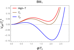
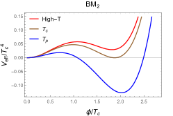
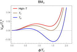
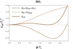
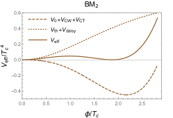
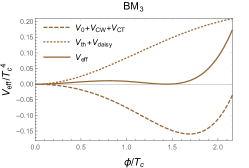
Figure 1: Top: Evolution of the vacuum for three benchmark points on the $V_{\rm eff}/T_{c}^{4}-\phi/T_{c}$ plane. The three temperatures are, respectively, some temperature higher than $T_{c}$ (red), the critical temperature $T_{c}$ (brown), and the percolation temperature $T_{p}$ (blue) as will be further explained in Section 4; Bottom: Components of the effective potential at $T_{c}$.

For illustration, we present the thermal effective potential at different temperatures for three benchmark points given in table 1, and illustrate in the top row of figure 1 how phase transition occurs. In each plot, $T_{c}$ represents the critical temperature, and $T_{p}$ is the percolation temperature whose definition will become clear in section 4. As seen from these plots, when the Universe cools down, the potential barrier would arise and suggest that the phase transition is of first order. Accordingly, we show in the bottom row of figure 1 the components of $V_{\rm eff}$ to clarify the fact that the barrier indeed comes from thermal corrections. Therefore, this kind of phase transition would belong to the thermally driven class of the electroweak phase transition Chung:2012vg . Moreover, our result shows that $V_{\rm th}$ ($V_{\rm daisy}$) contributes positively (negatively) to $V_{\rm eff}$ around the true vacua, while $V_{\rm th}+V_{\rm daisy}$ contributes a net positive correction to $V_{\rm eff}$. As a result, these two thermal corrections lift up the zero-temperature effective potential ($V_{0}+V_{\rm CW}+V_{CT}$) to an extent that helps form a maximum in the potential shape and yields the potential barrier around $\phi/T_{c}\sim 1$.

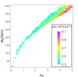
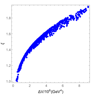
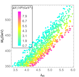
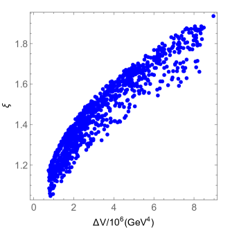
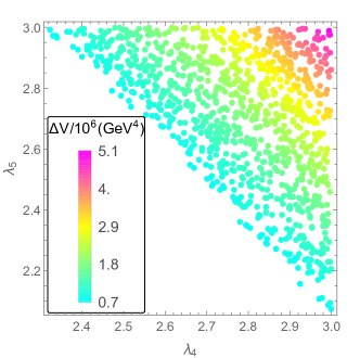
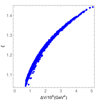
                                   (Setup 1)                                    (Setup 3)                                    (Setup 4)

Figure 2: The height of the potential barriers and the $\xi$ for various $\lambda_{45}$ and $M_{\Delta}$ for the four setups. Note that setup 2 is missing due to the fact that the decoupling of the heavy triplet.

To ensure the first-order phase transition is strong enough to avoid later time washout of the baryon numbers, one needs $\xi>1$ as discussed above. For a successful SFOEWPT in the type-II model, after performing the numerical calculations, we show our results in figure 2 for the four setups above, where the left column shows the results for the barrier height, and the right column for $\xi$. Note that the second setup is missing in our results due to the fact that the triplet scalars in this scenario are too heavy to contribute to the potential barrier and therefore decouple from the phase transition. For setup 1 and 3, the height of the barriers are only functions of $\lambda_{45}$ and $M_{\Delta}$. While for setup 4, since we fix $M_{\Delta}=500$ GeV, we plot the barrier height as a function of the individual $\lambda_{4,5}$ couplings instead. Clearly, our results show that large $\lambda_{4,5}$ and heavy $M_{\Delta}$ help increase the barrier height and therefore enhance the value of $\xi$ as seen from the second column of figure 2. However, we comment on that due to the decoupling effects, when $M_{\Delta}$ exceeds $\sim 550$ GeV, the barrier height would become insufficient to induce a SFOEWPT as implied in the first two plots in the left column of figure 2. Interestingly, most of the $\xi\geq 1$ viable points falls into the mass region that could be tested at current/future colliders Du:2018eaw , suggesting the possible synergy of different probes in searching for the type-II seesaw model. For each setup, we further discuss this possibility below.

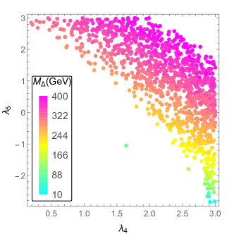
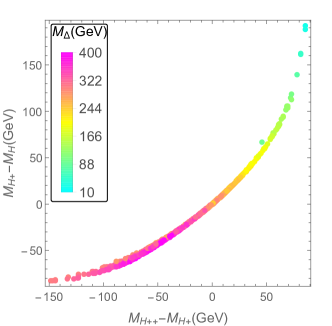
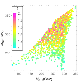
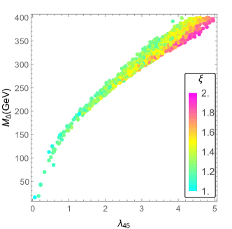
Figure 3: SFOEWPT viable benchmark points for our setup 1. In the upper row, we show benchmark points with $\xi>1$, while in the second row, we show explicitly the value of $\xi$ on different parameter planes. See the main text for details.

For setup 1, our results are shown in figure 3. The first plot in the upper row shows the benchmark points for a SFOEWPT with varying $M_{\Delta}$ and $\lambda_{4,5}$. Note that a light triplet with $M_{\Delta}\simeq 10$ GeV still permits a SFOEWPT and we comment on that the triplet mass eigenvalues are much larger than $M_{\Delta}$ in this case due to corrections from negative $\lambda_{5}$’s. See our eqs. (31) and (32), for example. However, we point out that since $v_{\Delta}$ is small in this case, the same-sign dilepton channel dominates the decay of $H^{\pm\pm}$ and one can thus utilize the $pp\rightarrow H^{++}H^{--}\rightarrow\ell^{+}\ell^{+}\ell^{\prime-}\ell^{\prime-}$ channel to constrain the light triplet scenario. See, for example, Ref. Du:2018eaw . Similarly, we show in the second plot in the first row of figure 3 for the benchmark points that can result in a SFOEWPT with different triplet mass differences. The mass differences are essentially only dependent on $\lambda_{5}$ since $v_{\Delta}\ll v_{\Phi}$ and $\sin\alpha\approx 0$. In this case, we find the parameter benchmark points are rather limited, suggesting the fact that one could possibly recast current/future experimental results onto the mass difference plane as we show here to determine the mass scale of the triplet and also $\lambda_{5}$. This in turn would help identify the triplet model and its model parameter determination at colliders.

On the other hand, the benchmark points for a SFOEWPT are shown in the bottom row of figure 3, where the colored legend indicates directly the value of $\xi$ for the phase transition. Note that the points mainly reside in the lower half of the $M_{H^{\pm}}-M_{H^{\pm\pm}}$ plane as seen from the first plot of the bottom row. In particular, $\xi$ approaches larger values when $200\lesssim M_{H^{\pm}}\lesssim 300$ GeV and $250\lesssim M_{H^{\pm\pm}}\lesssim 350$ GeV, indicating that positive $\lambda_{5}$’s are slightly favored for a SFOEWPT as is also clear in the first plot of the first row. Similarly, from the last plot in the last row of figure 3, one sees that positive $\lambda_{45}$ are preferred for a SFOEWPT, suggesting also a preference of positive $\lambda_{4}$’s that all together help stabilize the Higgs potential up to the Planck scale as observed in Ref. Du:2022vso .

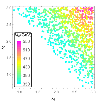
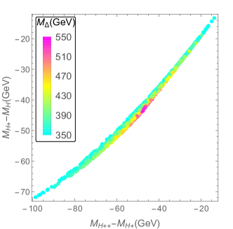
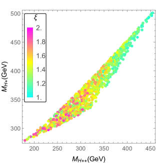
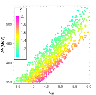
Figure 4: Same as figure 3 but for our setup 3.

A similar observation as discussed above applies to our setup 3, which can be seen directly from our figure  4. Note that in our setup 3, even though we scan over a relatively large range of $M_{\Delta}$ up to about 1 TeV, light triplet Higgs particles are generically preferred for a SFOEWPT as indicated by the dots in red/purple.

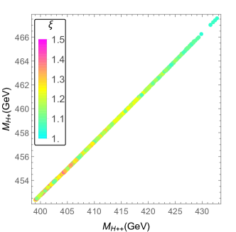
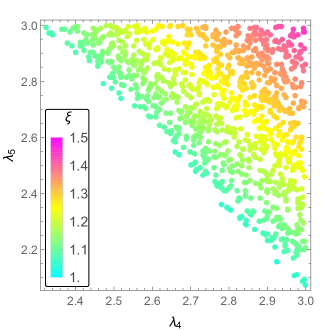
Figure 5: Left panel: same as the bottom-left of figure 3 but for our setup 4; Right panel: the explicitly value of $\xi$ on the plane of $\lambda_{4}$ and $\lambda_{5}$.

Finally, for our setup 4, the results are presented in figure 5. Note that in this case, we fix $M_{\Delta}=500$ GeV. This is motivated by the consideration that, upon model discovery, around this specific value for example, one can then readily recast the masses of the triplet Higgs particles onto the first panel of figure 5 to check the existence of a SFOEWPT. From the distribution of $\xi$, one can then utilize the second plot of figure 5 to possibly determine the sign of $\lambda_{4,5}$, and thus the mass spectrum of the triplet model. We comment on that for setup 4, we again find that positive $\lambda_{4,5}$ are preferred for a SFOEWPT.

3.6 Implications from Br($h\to\gamma\gamma$)

As already observed in Ref. Chao:2012mx ; Du:2018eaw , theoretical constraints on the portal couplings $\lambda_{4,5}$ are already very stringent, especially for those from one-loop perturbativity summarized in section 2.2.2. For this reason, we ask ourselves the following question: How could these points obtained in last subsection that are responsible for a SFOEWPT could be tested from current and/or future collider experiments?

To answer this question, we first map those points for each setup in section 3.5 onto the $\lambda_{4}-\lambda_{5}$ plane from considering vacuum stability, perturbative unitarity and perturbativity up to one loop. The results are shown in figure 6, where the left panel is from tree-level vacuum stability and perturbative unitarity, and the right one for one-loop perturbativity. The legend alongside the right panel indicates the scale to which one-loop perturbativity is satisfied. Clearly, from tree-level theoretical constraints as indicated in gray in the left panel of figure 6, positive $\lambda_{4}$ is in general preferred. This conclusion changes slightly when one-loop perturbativity is taken into account. In the latter case, requiring perturbativity up to the Planck scale, we find $\lambda_{4,5}$ with opposite signs near the origin are generically disfavored as implied by the elliptical region in the right panel.

The viable points that can lead to a SFOEWPT are then shown in black, blue, and red for setup 1, setup 3 and setup 4, respectively. Note that all the points fulfill tree-level constraints from perturbative unitarity and vacuum stability. Furthermore, even when one-loop perturbativity is taken into account, we find that all these points are still allowed up to the Planck scale as indicated in the right panel of figure 6.

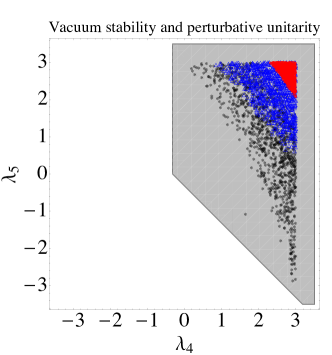
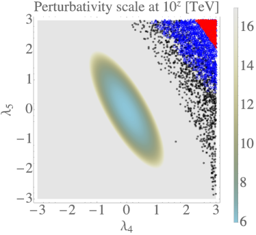
Figure 6: Left panel: Theoretical constraints on the triplet model from tree-level vacuum stability and perturbative unitarity. Right panel: Constraints from one-loop perturbativity. In each panel, the black, blue and red points correspond to our setup one, three and four, respectively.

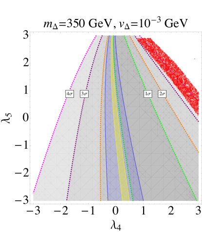
Figure 7: Precision measurements of $\mathcal{R}_{h\gamma\gamma}$ from current and future circular colliders. The green, orange, purple and magenta boundaries represent the $1\sigma$, $2\sigma$, $3\sigma$ and $4\sigma$ regions from Ref. ParticleDataGroup:2020ssz . The blue and the yellow regions are for a future 100 TeV collider FCC-ee and FCC-ee + FCC-pp, respectively. Our benchmark points are shown in the red.

On the other hand, from figures (3)-(5), we note that to have a successful SFOEWPT, the triplet masses are generically light such that they might be within the reach of current and future colliders. For instance, when the triplet is below $\sim$1 TeV, the same-sign dilepton (di-$W$ boson) channel would be the smoking-gun signature for discovering this model at colliders Du:2018eaw for small (large) $v_{\Delta}$. Therefore, to answer the question we raise earlier in this section, we make use of precision measurements of the $h\to\gamma\gamma$ decay rate defined as $\mathcal{R}_{h\gamma\gamma}\equiv\Gamma_{h\to\gamma\gamma}^{\rm NP}/\Gamma_{h\to\gamma\gamma}^{\rm SM}$, where $\Gamma_{h\to\gamma\gamma}^{\rm NP(SM)}$ is the $h\to\gamma\gamma$ decay rate with (without) the inclusion of new physics. Our benchmark scenario is obtained by fixing $m_{\Delta}$ at 350 GeV and $v_{\Delta}\simeq 10^{-3}$ GeV, and the result is shown in figure 7. The shaded region in gray corresponds to $\mathcal{R}_{h\gamma\gamma}=1.11^{+0.10}_{-0.09}$ from the most recent report of PDG ParticleDataGroup:2020ssz , whose $1\sigma$, $2\sigma$, $3\sigma$ and $4\sigma$ boundaries are given by the green, orange, purple and magenta dashed curves, respectively. For future circular colliders, we use the blue (yellow) region for a future 100 TeV FCC-ee (FCC-ee + FCC-pp) collider with $\mathcal{R}_{h\gamma\gamma}=1\pm 0.05\,(0.01)$ Contino:2016spe . The red circles in the upper right corner correspond to our benchmark points that can give a SFOEWPT within this setup.

Note that even though our benchmark points are still allowed within $3\sim 4\sigma$ from the current measurement of $\mathcal{R}_{h\gamma\gamma}$ in ParticleDataGroup:2020ssz , we expect the high-luminosity LHC and/or future colliders to scrutinize each of these benchmark points in this specific scenario, highlighting the powerfulness of precision measurements and the synergy of different probes.

4 Gravitational waves from the triplet model

As discussed in section 3, a SFOEWPT occurs when the temperature of the Universe drops below the critical temperature $T_{c}$. Gravitational waves (GWs) could then be generated through collisions of vacuum bubbles, and the interaction between bubbles and the thermal plasma. The generated GWs would then be possibly observed by late time observatories such as LISA LISA:2017pwj , TianQin TianQin:2015yph ; Hu:2018yqb ; TianQin:2020hid , Taiji Hu:2017mde ; Ruan:2018tsw , DECIGO Seto:2001qf ; Kudoh:2005as , and BBO Ungarelli:2005qb ; Cutler:2005qq . From this consideration, we discuss the synergy of different probes of the type-II seesaw model, and focus specifically on the observation of GWs in this section.

The spectrum of GWs from a first-order phase transition can be obtained quite systematically. See for example, Refs. Caprini:2019egz . Generically, the prediction of the GW spectrum depends on four key parameters: The bubble wall velocity $v_{w}$, the phase transition temperature, the latent heat $\Delta\rho$ released during the phase transition, the phase transition strength $\alpha$, and the phase transition duration $\beta$. The definitions and their physical meaning of these parameters will become clear shortly, as will be discussed below.

Below the critical temperature, the phase transition would take place when at least one bubble is nucleated per horizon volume and per horizon time, which can be defined as as Affleck:1980ac ; Linde:1981zj ; Linde:1980tt :

$$\Gamma\approx A(T_{n})e^{-S_{3}/T_{n}}\simeq 1\;.$$ (74)

where $T_{n}$ is the nucleation temperature of the vacuum bubbles, and $S_{3}$ is the bounce action for an O(3) symmetric bounce solution that can be written as

$$S_{3}(T)=\int 4\pi r^{2}dr\bigg{[}\frac{1}{2}\big{(}\frac{d\phi_{b}}{dr}\big{)}^{2}+V(\phi_{b},T)\bigg{]}\;,$$ (75)

with $\phi_{b}=\phi,\delta$ in our case, and $V(\phi_{b},T)$ the effective potential in eq. (50). The bubble nucleation events would be generated when one gets the bounce solution from solving the equations of motion for $\phi_{b}$:

$$\frac{d^{2}\phi_{b}}{dr^{2}}+\frac{2}{r}\frac{d\phi_{b}}{dr}-\frac{\partial V(\phi_{b})}{\partial\phi_{b}}=0\;,$$ (76)

with the boundary conditions being

$$\lim_{r\rightarrow\infty}\phi_{b}=0\;,\quad\quad{\left.{\frac{{d{\phi_{b}}}}{{dr}}}\right|_{r=0}}=0\;.$$ (77)

After nucleation, the phase transition proceeds through expansion and percolation of these vacuum bubbles. The percolation temperature $T_{p}$ is defined as the moment when the probability of the friction of a false vacuum is 0.7 Guth:1981uk ; Ellis:2018mja :

$$P[T_{p}]=e^{-I[T_{p}]}=0.7\;,$$

$$I[T]=\frac{4\pi v_{w}^{3}}{3}\int_{T}^{T_{c}}\frac{d\tilde{T}\Gamma(\tilde{T})}{H(\tilde{T})\tilde{T}^{4}}\left(\int_{T}^{\tilde{T}}\frac{dT^{\prime}}{H(T^{\prime})}\right)^{3}\;,$$ (78)

where $v_{w}$ is the bubble wall velocity.

For this study, we define the phase transition strength $\alpha$ as

$$\alpha=\frac{\Delta\rho}{\rho_{R}}\;,$$ (79)

where the radiation energy density of the bath or the plasma background $\rho_{R}$ is given by

$$\rho_{R}=\frac{\pi^{2}g_{\star}T_{\star}^{4}}{30}\;,$$ (80)

with $g_{\star}\approx 100$ being the effective number of degrees of freedom, $T_{\star}$ the plasma temperature that is approximately equivalent to the percolation temperature $T_{\star}\approx T_{p}$ for transitions without significant reheating Caprini:2015zlo , and $\Delta\rho$ the latent heat from the phase transition. $\Delta\rho$ can be calculated from the difference of the energy density between the false and the true vacuum, i.e., $\Delta\rho=\rho(\phi_{p},T_{p})-\rho(v_{p},T_{p})$, where

$$\rho(\phi_{p},T_{p}) = \left.-V(\phi,T)\right|_{T=T_{p}}+\left.T\frac{d\,V(\phi,T)}{d\,T}\right|_{T=T_{p}}\;,$$ (81)

$$\rho(v_{p},T_{p}) = -\left.V(h,T)\right|_{T=T_{p}}+\left.T\frac{d\,V(h,T)}{d\,T}\right|_{T=T_{p}}\;.$$ (82)

Here, we remind the reader that $\alpha$ and $\rho$ in this section represent the phase transition strength and the energy densities instead of the mixing angle and the electroweak parameter discussed in section 2. Finally, to characterizes the inverse time duration of the SFOEWPT, we define the parameter $\beta$ as

$$\frac{\beta}{H_{p}}=\left.T\frac{d(S_{3}(T)/T)}{dT}\right|_{T=T_{p}}\;,$$ (83)

with $H_{p}$ the Hubble constant at the percolation temperature $T_{p}$.

With above results, we are now ready to move to the discussion on the sources of GW generation from a first-order phase transition. In this work, we consider three sources for the production of GWs. The first one comes from the uncollided envelop of thin bubble walls during the bubble collision, while the collided thin bubble walls are assumed to disappear instantly after two bubbles overlap. This is the widely used envelop approximation that contributes to both numerical simulations Kosowsky:1991ua ; Kosowsky:1992rz ; Kosowsky:1992vn ; Kamionkowski:1993fg ; Huber:2008hg (see also Child:2012qg ) and analytic estimations Jinno:2016vai . The dimensionless energy density spectrum is fitted to be Huber:2008hg

$$\Omega h^{2}_{\rm coll}(f)=1.67\times 10^{-5}\left(\frac{100}{g_{*}}\right)^{\frac{1}{3}}\left(\frac{\beta}{H}\right)^{-2}\left(\frac{\kappa_{\phi}\alpha}{1+\alpha}\right)^{2}\frac{0.11v_{w}^{3}}{0.42+v_{w}^{2}}\frac{3.8\left(f/f_{\rm coll}\right)^{2.8}}{1+2.8\left(f/f_{\rm coll}\right)^{3.8}},$$ (84)

where the first term in bracket accounts for the redshift effect, the second one reflects its scaling behavior, and the third one parameterizes the spectral shape of the GW radiation. The peak frequency $f_{\rm coll}$ involved in the spectral shape is fitted to be Huber:2008hg

$$f_{\rm coll}=1.65\times 10^{-5}\,\mathrm{Hz}\times\left(\frac{g_{*}}{100}\right)^{\frac{1}{6}}\frac{T_{\star}}{100\mathrm{GeV}}\frac{0.62}{1.8-0.1v_{w}+v_{w}^{2}}\left(\frac{\beta}{H_{\ast}}\right).$$ (85)

The other two sources for GW production during the EWPT we consider are: (1) the sound waves in the plasma Hindmarsh:2013xza ; Hindmarsh:2015qta , and (2) the magnetohydrodynamic turbulence (MHD) Hindmarsh:2013xza ; Hindmarsh:2015qta . For the former, taking the lifetime suppression factor obtained in Guo:2020grp , the energy density spectrum from the sound waves can be expressed as Hindmarsh:2015qta ,

$$\Omega h^{2}_{\rm sw}(f)=1.64\times 10^{-6} \times(H_{*}\tau_{sw})\left(\frac{\beta}{H}\right)^{-1}\left(\frac{\kappa\alpha}{1+\alpha}\right)^{2}\left(\frac{g_{*}}{100}\right)^{-\frac{1}{3}}$$

$$\times v_{w}(8\pi)^{1/3}\left(\frac{f}{f_{\rm sw}}\right)^{3}\left(\frac{7}{4+3\left(f/f_{\rm sw}\right)^{2}}\right)^{7/2},$$ (86)

with $\tau_{sw}={\rm min}\left(\frac{1}{H_{*}},\frac{R_{*}}{\bar{U}_{f}}\right)$, $H_{*}R_{*}=v_{w}(8\pi)^{1/3}(\beta/H)^{-1}$. Here, $\bar{U}$ is the root-mean-square fluid velocity that can be approximated as Hindmarsh:2017gnf ; Caprini:2019egz ; Ellis:2019oqb

$$\bar{U}_{f}^{2}\approx\frac{3}{4}\frac{\kappa_{\nu}\alpha}{1+\alpha}\;,$$ (87)

and again, $\alpha$ here is the phase transition strength. The term $H_{*}\tau_{\rm sw}$ in eq. (4) accounts for the suppression of the GW amplitude for sound waves if the sound wave source could not last longer than one Hubble time, and $H_{\ast}$ is the Hubble parameter at the temperature $T_{\ast}$. Practically, $T_{\ast}$ is very close to $T_{p}$, and for this reason, we replace $T_{\ast}$ by $T_{p}$ in the our calculations. $\kappa_{v}$ is the fraction of the released energy into the kinetic energy of the plasma, which can be calculated given $v_{w}$ and $\alpha$ Espinosa:2010hh . Finally $f_{\text{sw}}$ is the peak frequency of above energy density spectrum:

$$f_{\textrm{sw}}=1.9\times 10^{-5}\frac{1}{v_{w}}\left(\frac{\beta}{H_{\ast}}\right)\left(\frac{T_{\ast}}{100\textrm{GeV}}\right)\left(\frac{g_{\ast}}{100}\right)^{1/6}\textrm{Hz}.$$ (88)

On the other hand, for the latter source of GW production, it arises from the fact that a small fraction of the energy would flow into the MHD. Its contribution to the energy density spectrum can be expressed as Caprini:2009yp ; Binetruy:2012ze

$$\Omega_{\textrm{turb}}h^{2}= \,3.35\times 10^{-4}\left(\frac{\beta}{H_{\ast}}\right)^{-1}\left(\frac{\kappa_{\text{turb}}\alpha}{1+\alpha}\right)^{3/2}\left(\frac{100}{g_{\ast}}\right)^{1/3}$$

$$\,\times v_{w}\cdot\frac{(f/f_{\textrm{turb}})^{3}}{[1+(f/f_{\textrm{turb}})]^{11/3}(1+8\pi f/h_{\ast})}\;,\quad$$ (89)

where the factor $\kappa_{\text{turb}}$ is the fraction of energy transferred to the MHD turbulence and can be roughly estimated as $\kappa_{\text{turb}}\approx\epsilon\kappa_{v}$ with $\epsilon\approx$ 5 $\sim$ 10% Hindmarsh:2015qta . In this work, we take $\epsilon\approx 0.1$ for the following discussion. Similar to $f_{\text{sw}}$, $f_{\text{turb}}$ is the peak frequency for the spectrum from the MHD:

$$f_{\textrm{turb}}=2.7\times 10^{-5}\frac{1}{v_{w}}\left(\frac{\beta}{H_{\ast}}\right)\left(\frac{T_{\ast}}{100\textrm{GeV}}\right)\left(\frac{g_{\ast}}{100}\right)^{1/6}\textrm{Hz}.$$ (90)

		$T_{p}$(GeV)	$\alpha[T_{p}]$	$\beta/H[T_{p}]$
setup 1	${\rm BM}_{1}$	96.701	0.048	657.743
setup 3	${\rm BM}_{2}$	99.195	0.046	1026.894
setup 4	${\rm BM}_{3}$	136.708	0.015	2712.428

Table 2: Three benchmark points for the illustration of GW production from a SFOEWPT for the setup 1, 3, and 4. Setup 2 is missing in this table due to the decoupling.

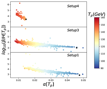
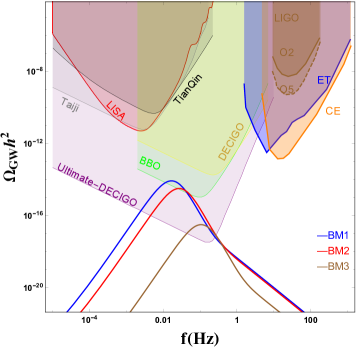
Figure 8: Left: $\beta/H[T_{p}]$ and $\alpha$ for the four benchmark setups in section 3.5. Note that setup 2 is missing due to the decoupling of the triplet. The legend along with the figure is used to indicate the percolation temperature $T_{p}$, and the black stars denote three benchmark points in table 2. Right: The representative GW signal spectrum for the three benchmark points in table 2. See the main text for details.

The predicted GW spectrum can then be readily calculated from the three sources discussed above, leading to

$$\Omega_{\rm GW}h^{2}=\Omega h^{2}_{\rm coll}(f)+\Omega h^{2}_{\rm sw}(f)+\Omega_{\textrm{turb}}h^{2}\;.$$ (91)

This predicted spectrum could then be tested at various GW observatories mentioned above, thus it could also be used for discovering/testing specific UV models like the type-II seesaw model considered in this work. To that end, we choose three benchmark points for the four setups discussed in section 3.5 and comment on the fact that no benchmark points are selected for the second setup due to the decoupling discussed earlier. The selected benchmark points for the rest three setups are then summarized in table 2, whose effective potential have been presented in figure 1 and their corresponding results for GWs are presented in figure 8.

In the left panel of figure 8, we show the results for $\beta/H[T_{p}]$ and $\alpha[T_{p}]$ for varying percolation temperatures. Note that, as self-explained in eqs. (84), (4), and (89), the magnitude of GWs is inversely proportional to $\beta/H_{\star}$ and directly proportional to $\alpha$ for fixed $v_{w}$ and $T_{\star}$. As a result, one naturally expects that a larger value of $\alpha$ and/or a smaller value of $\beta/H_{\star}$ would lead to an increase in the magnitude of the GWs observed. This is as expected since a larger value of $\alpha$ would suggest more energy transition from the plasma to the form of GWs. Similarly, a smaller $\beta/H_{\star}$ would imply a longer period for the strong first-order phase transition, thus also enhancing the magnitude of the spectrum. This is also confirmed numerically as shown in the right panel of figure 8.

The predicted spectra for the three benchmark points in table 2 are presented in blue, red and orange in the right panel of figure 8, respectively. These three benchmarks are chosen with relatively large $\alpha$ and small $\beta/H_{\star}$ from the left panel of figure 8 to enhance the magnitude of the generated GWs. See the corresponding black stars in the left panel for these three benchmark points we choose. As a result, we find the generated GW waves from the SFOEWPT all have a peak frequency within the $0.01\sim 0.1$Hz range, with the peak yields of the GWs around $10^{-14}$, $10^{-15.5}$ and $10^{-16.5}$ for our BM1 (blue), BM2 (red), and BM3 (brown), respectively. From the right panel of figure 8, we comment on that while the peak yields of the GWs for our BM2 and BM3 are small, they would be covered by Ultimate-DECIGO in the future. In particular, we see that BBO would be able to explore the edge of the BM1 scenario, and the Ultimate-DECIGO would have the chance to further examine both the BM1 and the BM2 cases.

5 Conclusions

Neutrino masses and the baryon asymmetry of the Universe both indicate new physics beyond the SM. In this work, we focus on the type-II seesaw model that acts as a possible candidate for answering these two questions simultaneously. Specifically, the type-II seesaw model can be obtained by extending the SM Higgs sector with a complex triplet that transforms as $(1,3,2)$ under the SM gauge group. Due to the quantum numbers of the triplet, new interactions are introduced between the SM Higgs doublet and the complex triplet, such that the SM Higgs potential could be modified in a way such that a SFOEWPT is possible.

We study the phase transition within the triplet model in detail in this work and obtain viable regions of the model parameter space for a SFOEWPT that is responsible for explaining the observed baryon asymmetry. Our results are shown in figures 2-5 for the four setups discussed in section 3. We find that when the triplet is heavy above $\sim 550$ GeV, effects on the Higgs potential from the triplet would decouple such that a SFOEWPT would become absent in this model. Furthermore, we conclude from our study that a SFOEWPT generically prefers positive values for the Higgs portal couplings $\lambda_{4,5}$, which in turn help stabilize the Higgs potential up to the Planck scale up to one-loop level Du:2022vso . We point out that the Higgs di-photon decay rate is also sensitive to $\lambda_{4,5}$ Du:2018eaw , such that a precision measurement on the rate could shed some light on the phase transition. This highlights the synergy of different probes in searching for new physics.

On the other hand, gravitational waves can be also generated during the SFOEWPT from bubble collisions and its interaction with thermal plasma. This has been investigated in section 4 in the complex triplet model, and the results are presented in our figure 8. For the four setups we consider that cover the model parameter space up to 4 TeV, we obtain the phase transition strength $\alpha$ and the phase transition duration $\beta$ for various percolation temperatures. Based on that, we then choose three optimistic benchmark points to calculate the gravitational wave yields and compare them with different observatories now and in the future. We find the peak frequency of the gravitational waves could be within the 0.01$\sim$0.1 Hz range, with a peak yield of gravitational waves at the edge of BBO and could be further examined in the future by Ultimate-DECIGO.

Last but not least, we comment that, for a successful first-order phase transition and a relatively large yield of gravitational waves, we observe that the triplet Higgs particles are preferred to be light below the TeV scale. With the triplet particles being light at such a scale, the triplet vev would need to be large above $\sim 10^{-4}$ GeV to avoid very stringent constraints from current collider searches ATLAS:2017xqs ; Du:2018eaw . This in turn would result in tiny neutrino Yukawa couplings due to the tininess of neutrino masses. As a consequence, one would thus expect the triplet model not to manifest itself in foreseen neutrino oscillation experiments due to the neutrino Yukawa suppression. However, collider searches would help with the same-sign di-$W$ boson final state being the smoking-gun signature.

- (1) ATLAS Collaboration, G. Aad et al., Observation of a new particle in the search for the Standard Model Higgs boson with the ATLAS detector at the LHC, Phys. Lett. B 716 (2012) 1–29, [arXiv:1207.7214].
- (2) CMS Collaboration, S. Chatrchyan et al., Observation of a New Boson at a Mass of 125 GeV with the CMS Experiment at the LHC, Phys. Lett. B 716 (2012) 30–61, [arXiv:1207.7235].
- (3) Super-Kamiokande Collaboration, Y. Fukuda et al., Evidence for oscillation of atmospheric neutrinos, Phys. Rev. Lett. 81 (1998) 1562–1567, [hep-ex/9807003].
- (4) SNO Collaboration, Q. R. Ahmad et al., Measurement of the rate of interactions produced by solar neutrinos at the Sudbury Neutrino Observatory, Phys. Rev. Lett. 87 (2001) 071301, [nucl-ex/0106015].
- (5) K. Kajantie, M. Laine, K. Rummukainen, and M. E. Shaposhnikov, The Electroweak phase transition: A Nonperturbative analysis, Nucl. Phys. B 466 (1996) 189–258, [hep-lat/9510020].
- (6) K. Kajantie, M. Laine, K. Rummukainen, and M. E. Shaposhnikov, Is there a hot electroweak phase transition at ?, Phys. Rev. Lett. 77 (1996) 2887–2890, [hep-ph/9605288].
- (7) K. Kajantie, M. Laine, K. Rummukainen, and M. E. Shaposhnikov, A Nonperturbative analysis of the finite T phase transition in SU(2) x U(1) electroweak theory, Nucl. Phys. B 493 (1997) 413–438, [hep-lat/9612006].
- (8) Planck Collaboration, N. Aghanim et al., Planck 2018 results. VI. Cosmological parameters, Astron. Astrophys. 641 (2020) A6, [arXiv:1807.06209]. [Erratum: Astron.Astrophys. 652, C4 (2021)].
- (9) P. Minkowski, at a Rate of One Out of Muon Decays?, Phys. Lett. 67B (1977) 421–428.
- (10) P. Ramond, The Family Group in Grand Unified Theories, in International Symposium on Fundamentals of Quantum Theory and Quantum Field Theory Palm Coast, Florida, February 25-March 2, 1979, pp. 265–280, 1979. hep-ph/9809459.
- (11) M. Gell-Mann, P. Ramond, and R. Slansky, Complex Spinors and Unified Theories, Conf. Proc. C790927 (1979) 315–321, [arXiv:1306.4669].
- (12) T. Yanagida, HORIZONTAL SYMMETRY AND MASSES OF NEUTRINOS, Conf. Proc. C7902131 (1979) 95–99.
- (13) R. N. Mohapatra and G. Senjanovic, Neutrino Mass and Spontaneous Parity Violation, Phys. Rev. Lett. 44 (1980) 912.
- (14) J. Schechter and J. W. F. Valle, Neutrino Masses in SU(2) x U(1) Theories, Phys. Rev. D22 (1980) 2227.
- (15) J. Schechter and J. W. F. Valle, Neutrino Decay and Spontaneous Violation of Lepton Number, Phys. Rev. D25 (1982) 774.
- (16) W. Konetschny and W. Kummer, Nonconservation of Total Lepton Number with Scalar Bosons, Phys. Lett. 70B (1977) 433–435.
- (17) T. P. Cheng and L.-F. Li, Neutrino Masses, Mixings and Oscillations in SU(2) x U(1) Models of Electroweak Interactions, Phys. Rev. D22 (1980) 2860.
- (18) G. Lazarides, Q. Shafi, and C. Wetterich, Proton Lifetime and Fermion Masses in an SO(10) Model, Nucl. Phys. B181 (1981) 287–300.
- (19) M. Magg and C. Wetterich, Neutrino Mass Problem and Gauge Hierarchy, Phys. Lett. 94B (1980) 61–64.
- (20) R. Foot, H. Lew, X. G. He, and G. C. Joshi, Seesaw Neutrino Masses Induced by a Triplet of Leptons, Z. Phys. C44 (1989) 441.
- (21) E. Witten, New Issues in Manifolds of SU(3) Holonomy, Nucl. Phys. B268 (1986) 79.
- (22) R. N. Mohapatra, Mechanism for Understanding Small Neutrino Mass in Superstring Theories, Phys. Rev. Lett. 56 (1986) 561–563.
- (23) R. N. Mohapatra and J. W. F. Valle, Neutrino Mass and Baryon Number Nonconservation in Superstring Models, Phys. Rev. D34 (1986) 1642.
- (24) J. W. F. Valle NUCLEAR BETA DECAYS AND NEUTRINO: proceedings. Edited by T. Kotani, H. Ejiri, E. Takasugi, Singapore, (1986) 542p.
- (25) S. M. Barr, A Different seesaw formula for neutrino masses, Phys. Rev. Lett. 92 (2004) 101601, [hep-ph/0309152].
- (26) R. N. Mohapatra and G. Senjanovic, Neutrino Masses and Mixings in Gauge Models with Spontaneous Parity Violation, Phys. Rev. D23 (1981) 165.
- (27) S. Weinberg, Baryon and Lepton Nonconserving Processes, Phys. Rev. Lett. 43 (1979) 1566–1570.
- (28) T. Han and B. Zhang, Signatures for Majorana neutrinos at hadron colliders, Phys. Rev. Lett. 97 (2006) 171804, [hep-ph/0604064].
- (29) A. Atre, T. Han, S. Pascoli, and B. Zhang, The Search for Heavy Majorana Neutrinos, JHEP 05 (2009) 030, [arXiv:0901.3589].
- (30) P. Fileviez Perez, T. Han, and T. Li, Testability of Type I Seesaw at the CERN LHC: Revealing the Existence of the B-L Symmetry, Phys. Rev. D 80 (2009) 073015, [arXiv:0907.4186].
- (31) D. Alva, T. Han, and R. Ruiz, Heavy Majorana neutrinos from fusion at hadron colliders, JHEP 02 (2015) 072, [arXiv:1411.7305].
- (32) Y. Cai, T. Han, T. Li, and R. Ruiz, Lepton Number Violation: Seesaw Models and Their Collider Tests, Front. in Phys. 6 (2018) 40, [arXiv:1711.02180].
- (33) P. S. B. Dev, M. J. Ramsey-Musolf, and Y. Zhang, Doubly-Charged Scalars in the Type-II Seesaw Mechanism: Fundamental Symmetry Tests and High-Energy Searches, Phys. Rev. D 98 (2018), no. 5 055013, [arXiv:1806.08499].
- (34) Y. Du, A. Dunbrack, M. J. Ramsey-Musolf, and J.-H. Yu, Type-II Seesaw Scalar Triplet Model at a 100 TeV Collider: Discovery and Higgs Portal Coupling Determination, JHEP 01 (2019) 101, [arXiv:1810.09450].
- (35) L. Niemi, H. H. Patel, M. J. Ramsey-Musolf, T. V. I. Tenkanen, and D. J. Weir, Electroweak phase transition in the real triplet extension of the SM: Dimensional reduction, Phys. Rev. D 100 (2019), no. 3 035002, [arXiv:1802.10500].
- (36) R. Zhou, W. Cheng, X. Deng, L. Bian, and Y. Wu, Electroweak phase transition and Higgs phenomenology in the Georgi-Machacek model, JHEP 01 (2019) 216, [arXiv:1812.06217].
- (37) L. Bian, H.-K. Guo, Y. Wu, and R. Zhou, Gravitational wave and collider searches for electroweak symmetry breaking patterns, Phys. Rev. D 101 (2020), no. 3 035011, [arXiv:1906.11664].
- (38) A. Addazi, A. Marcianò, A. P. Morais, R. Pasechnik, R. Srivastava, and J. W. F. Valle, Gravitational footprints of massive neutrinos and lepton number breaking, Phys. Lett. B 807 (2020) 135577, [arXiv:1909.09740].
- (39) L. Niemi, M. J. Ramsey-Musolf, T. V. I. Tenkanen, and D. J. Weir, Thermodynamics of a Two-Step Electroweak Phase Transition, Phys. Rev. Lett. 126 (2021), no. 17 171802, [arXiv:2005.11332].
- (40) OPAL Collaboration, P. D. Acton et al., A Search for doubly charged Higgs production in Z0 decays, Phys. Lett. B 295 (1992) 347–356.
- (41) OPAL Collaboration, G. Abbiendi et al., Search for doubly charged Higgs bosons with the OPAL detector at LEP, Phys. Lett. B 526 (2002) 221–232, [hep-ex/0111059].
- (42) C.-W. Chiang, G. Cottin, Y. Du, K. Fuyuto, and M. J. Ramsey-Musolf, Collider Probes of Real Triplet Scalar Dark Matter, JHEP 01 (2021) 198, [arXiv:2003.07867].
- (43) N. F. Bell, M. J. Dolan, L. S. Friedrich, M. J. Ramsey-Musolf, and R. R. Volkas, Two-Step Electroweak Symmetry-Breaking: Theory Meets Experiment, JHEP 05 (2020) 050, [arXiv:2001.05335].
- (44) E. Hall, R. McGehee, H. Murayama, and B. Suter, Asymmetric Dark Matter May Not Be Light, arXiv:2107.03398.
- (45) CDF Collaboration, T. Aaltonen et al., Search for new physics in high like-sign dilepton events at CDF II, Phys. Rev. Lett. 107 (2011) 181801, [arXiv:1108.0101].
- (46) ATLAS Collaboration, G. Aad et al., Search for anomalous production of prompt like-sign muon pairs and constraints on physics beyond the Standard Model with the ATLAS detector, Phys. Rev. D85 (2012) 032004, [arXiv:1201.1091].
- (47) ATLAS Collaboration, G. Aad et al., Search for anomalous production of prompt like-sign lepton pairs at TeV with the ATLAS detector, JHEP 12 (2012) 007, [arXiv:1210.4538].
- (48) ATLAS Collaboration, G. Aad et al., Search for doubly-charged Higgs bosons in like-sign dilepton final states at TeV with the ATLAS detector, Eur. Phys. J. C72 (2012) 2244, [arXiv:1210.5070].
- (49) ATLAS Collaboration, G. Aad et al., Search for new phenomena in events with three or more charged leptons in collisions at TeV with the ATLAS detector, JHEP 08 (2015) 138, [arXiv:1411.2921].
- (50) ATLAS Collaboration, G. Aad et al., Search for anomalous production of prompt same-sign lepton pairs and pair-produced doubly charged Higgs bosons with TeV collisions using the ATLAS detector, JHEP 03 (2015) 041, [arXiv:1412.0237].
- (51) ATLAS Collaboration, G. Aad et al., Search for heavy long-lived multi-charged particles in pp collisions at TeV using the ATLAS detector, Eur. Phys. J. C75 (2015) 362, [arXiv:1504.04188].
- (52) CMS Collaboration, A. M. Sirunyan et al., Observation of electroweak production of same-sign W boson pairs in the two jet and two same-sign lepton final state in proton-proton collisions at 13 TeV, Phys. Rev. Lett. 120 (2018), no. 8 081801, [arXiv:1709.05822].
- (53) ATLAS Collaboration, M. Aaboud et al., Search for doubly charged Higgs boson production in multi-lepton final states with the ATLAS detector using proton–proton collisions at , Eur. Phys. J. C78 (2018), no. 3 199, [arXiv:1710.09748].
- (54) M. E. Machacek and M. T. Vaughn, Two Loop Renormalization Group Equations in a General Quantum Field Theory. 1. Wave Function Renormalization, Nucl. Phys. B 222 (1983) 83–103.
- (55) M. E. Machacek and M. T. Vaughn, Two Loop Renormalization Group Equations in a General Quantum Field Theory. 2. Yukawa Couplings, Nucl. Phys. B 236 (1984) 221–232.
- (56) M. E. Machacek and M. T. Vaughn, Two Loop Renormalization Group Equations in a General Quantum Field Theory. 3. Scalar Quartic Couplings, Nucl. Phys. B 249 (1985) 70–92.
- (57) H. Arason, D. J. Castano, B. Keszthelyi, S. Mikaelian, E. J. Piard, P. Ramond, and B. D. Wright, Renormalization group study of the standard model and its extensions. 1. The Standard model, Phys. Rev. D 46 (1992) 3945–3965.
- (58) C. Ford, I. Jack, and D. R. T. Jones, The Standard model effective potential at two loops, Nucl. Phys. B 387 (1992) 373–390, [hep-ph/0111190]. [Erratum: Nucl.Phys.B 504, 551–552 (1997)].
- (59) V. D. Barger, M. S. Berger, and P. Ohmann, Supersymmetric grand unified theories: Two loop evolution of gauge and Yukawa couplings, Phys. Rev. D 47 (1993) 1093–1113, [hep-ph/9209232].
- (60) M.-x. Luo and Y. Xiao, Two loop renormalization group equations in the standard model, Phys. Rev. Lett. 90 (2003) 011601, [hep-ph/0207271].
- (61) W. Chao and H. Zhang, One-loop renormalization group equations of the neutrino mass matrix in the triplet seesaw model, Phys. Rev. D 75 (2007) 033003, [hep-ph/0611323].
- (62) M. A. Schmidt, Renormalization group evolution in the type I+ II seesaw model, Phys. Rev. D 76 (2007) 073010, [arXiv:0705.3841]. [Erratum: Phys.Rev.D 85, 099903 (2012)].
- (63) P. Dey, A. Kundu, and B. Mukhopadhyaya, Some consequences of a Higgs triplet, J. Phys. G 36 (2009) 025002, [arXiv:0802.2510].
- (64) A. Arhrib, R. Benbrik, M. Chabab, G. Moultaka, M. C. Peyranere, L. Rahili, and J. Ramadan, The Higgs Potential in the Type II Seesaw Model, Phys. Rev. D 84 (2011) 095005, [arXiv:1105.1925].
- (65) W. Chao, M. Gonderinger, and M. J. Ramsey-Musolf, Higgs Vacuum Stability, Neutrino Mass, and Dark Matter, Phys. Rev. D 86 (2012) 113017, [arXiv:1210.0491].
- (66) E. J. Chun, H. M. Lee, and P. Sharma, Vacuum Stability, Perturbativity, EWPD and Higgs-to-diphoton rate in Type II Seesaw Models, JHEP 11 (2012) 106, [arXiv:1209.1303].
- (67) C. Bonilla, R. M. Fonseca, and J. W. F. Valle, Consistency of the triplet seesaw model revisited, Phys. Rev. D 92 (2015), no. 7 075028, [arXiv:1508.02323].
- (68) N. Haba, H. Ishida, N. Okada, and Y. Yamaguchi, Vacuum stability and naturalness in type-II seesaw, Eur. Phys. J. C 76 (2016), no. 6 333, [arXiv:1601.05217].
- (69) T. Li, Type II Seesaw and tau lepton at the HL-LHC, HE-LHC and FCC-hh, JHEP 09 (2018) 079, [arXiv:1802.00945].
- (70) P. Agrawal, M. Mitra, S. Niyogi, S. Shil, and M. Spannowsky, Probing the Type-II Seesaw Mechanism through the Production of Higgs Bosons at a Lepton Collider, Phys. Rev. D 98 (2018), no. 1 015024, [arXiv:1803.00677].
- (71) A. D. Sakharov, Violation of CP Invariance, C asymmetry, and baryon asymmetry of the universe, Pisma Zh. Eksp. Teor. Fiz. 5 (1967) 32–35.
- (72) V. A. Kuzmin, V. A. Rubakov, and M. E. Shaposhnikov, On the Anomalous Electroweak Baryon Number Nonconservation in the Early Universe, Phys. Lett. B 155 (1985) 36.
- (73) A. G. Cohen, D. B. Kaplan, and A. E. Nelson, Baryogenesis at the weak phase transition, Nucl. Phys. B 349 (1991) 727–742.
- (74) A. G. Cohen, D. B. Kaplan, and A. E. Nelson, Progress in electroweak baryogenesis, Ann. Rev. Nucl. Part. Sci. 43 (1993) 27–70, [hep-ph/9302210].
- (75) M. Quiros, Field theory at finite temperature and phase transitions, Helv. Phys. Acta 67 (1994) 451–583.
- (76) V. A. Rubakov and M. E. Shaposhnikov, Electroweak baryon number nonconservation in the early universe and in high-energy collisions, Usp. Fiz. Nauk 166 (1996) 493–537, [hep-ph/9603208].
- (77) K. Funakubo, CP violation and baryogenesis at the electroweak phase transition, Prog. Theor. Phys. 96 (1996) 475–520, [hep-ph/9608358].
- (78) M. Trodden, Electroweak baryogenesis, Rev. Mod. Phys. 71 (1999) 1463–1500, [hep-ph/9803479].
- (79) W. Bernreuther, CP violation and baryogenesis, Lect. Notes Phys. 591 (2002) 237–293, [hep-ph/0205279].
- (80) D. E. Morrissey and M. J. Ramsey-Musolf, Electroweak baryogenesis, New J. Phys. 14 (2012) 125003, [arXiv:1206.2942].
- (81) P. Di Bari, A. Masiero, and R. Mohapatra, Focus on the origin of matter, New J. Phys. 15 (2013) 035030.
- (82) LIGO Scientific, Virgo Collaboration, B. P. Abbott et al., Observation of Gravitational Waves from a Binary Black Hole Merger, Phys. Rev. Lett. 116 (2016), no. 6 061102, [arXiv:1602.03837].
- (83) LIGO Scientific, Virgo Collaboration, B. P. Abbott et al., GW170817: Observation of Gravitational Waves from a Binary Neutron Star Inspiral, Phys. Rev. Lett. 119 (2017), no. 16 161101, [arXiv:1710.05832].
- (84) LIGO Scientific, Virgo Collaboration, B. P. Abbott et al., GWTC-1: A Gravitational-Wave Transient Catalog of Compact Binary Mergers Observed by LIGO and Virgo during the First and Second Observing Runs, Phys. Rev. X 9 (2019), no. 3 031040, [arXiv:1811.12907].
- (85) LIGO Scientific, Virgo Collaboration, R. Abbott et al., GWTC-2: Compact Binary Coalescences Observed by LIGO and Virgo During the First Half of the Third Observing Run, Phys. Rev. X 11 (2021) 021053, [arXiv:2010.14527].
- (86) A. Mazumdar and G. White, Review of cosmic phase transitions: their significance and experimental signatures, Rept. Prog. Phys. 82 (2019), no. 7 076901, [arXiv:1811.01948].
- (87) C. Caprini et al., Detecting gravitational waves from cosmological phase transitions with LISA: an update, JCAP 03 (2020) 024, [arXiv:1910.13125].
- (88) LISA Collaboration, P. Amaro-Seoane et al., Laser Interferometer Space Antenna, arXiv:1702.00786.
- (89) TianQin Collaboration, J. Luo et al., TianQin: a space-borne gravitational wave detector, Class. Quant. Grav. 33 (2016), no. 3 035010, [arXiv:1512.02076].
- (90) X.-C. Hu, X.-H. Li, Y. Wang, W.-F. Feng, M.-Y. Zhou, Y.-M. Hu, S.-C. Hu, J.-W. Mei, and C.-G. Shao, Fundamentals of the orbit and response for TianQin, Class. Quant. Grav. 35 (2018), no. 9 095008, [arXiv:1803.03368].
- (91) TianQin Collaboration, J. Mei et al., The TianQin project: current progress on science and technology, PTEP 2021 (2021), no. 5 05A107, [arXiv:2008.10332].
- (92) W.-R. Hu and Y.-L. Wu, The Taiji Program in Space for gravitational wave physics and the nature of gravity, Natl. Sci. Rev. 4 (2017), no. 5 685–686.
- (93) W.-H. Ruan, Z.-K. Guo, R.-G. Cai, and Y.-Z. Zhang, Taiji program: Gravitational-wave sources, Int. J. Mod. Phys. A 35 (2020), no. 17 2050075, [arXiv:1807.09495].
- (94) N. Seto, S. Kawamura, and T. Nakamura, Possibility of direct measurement of the acceleration of the universe using 0.1-Hz band laser interferometer gravitational wave antenna in space, Phys. Rev. Lett. 87 (2001) 221103, [astro-ph/0108011].
- (95) H. Kudoh, A. Taruya, T. Hiramatsu, and Y. Himemoto, Detecting a gravitational-wave background with next-generation space interferometers, Phys. Rev. D 73 (2006) 064006, [gr-qc/0511145].
- (96) C. Ungarelli, P. Corasaniti, R. A. Mercer, and A. Vecchio, Gravitational waves, inflation and the cosmic microwave background: Towards testing the slow-roll paradigm, Class. Quant. Grav. 22 (2005) S955–S964, [astro-ph/0504294].
- (97) C. Cutler and J. Harms, BBO and the neutron-star-binary subtraction problem, Phys. Rev. D 73 (2006) 042001, [gr-qc/0511092].
- (98) L. Badurina et al., AION: An Atom Interferometer Observatory and Network, JCAP 05 (2020) 011, [arXiv:1911.11755].
- (99) AEDGE Collaboration, Y. A. El-Neaj et al., AEDGE: Atomic Experiment for Dark Matter and Gravity Exploration in Space, EPJ Quant. Technol. 7 (2020) 6, [arXiv:1908.00802].
- (100) L. Badurina, O. Buchmueller, J. Ellis, M. Lewicki, C. McCabe, and V. Vaskonen, Prospective sensitivities of atom interferometers to gravitational waves and ultralight dark matter, Phil. Trans. A. Math. Phys. Eng. Sci. 380 (2021), no. 2216 20210060, [arXiv:2108.02468].
- (101) V. Brdar, L. Graf, A. J. Helmboldt, and X.-J. Xu, Gravitational Waves as a Probe of Left-Right Symmetry Breaking, JCAP 12 (2019) 027, [arXiv:1909.02018].
- (102) V. Brdar, A. J. Helmboldt, and J. Kubo, Gravitational Waves from First-Order Phase Transitions: LIGO as a Window to Unexplored Seesaw Scales, JCAP 02 (2019) 021, [arXiv:1810.12306].
- (103) N. Okada and O. Seto, Probing the seesaw scale with gravitational waves, Phys. Rev. D 98 (2018), no. 6 063532, [arXiv:1807.00336].
- (104) L. Bian, W. Cheng, H.-K. Guo, and Y. Zhang, Cosmological implications of a B L charged hidden scalar: leptogenesis and gravitational waves, Chin. Phys. C 45 (2021), no. 11 113104, [arXiv:1907.13589].
- (105) M. Li, Q.-S. Yan, Y. Zhang, and Z. Zhao, Prospects of gravitational waves in the minimal left-right symmetric model, JHEP 03 (2021) 267, [arXiv:2012.13686].
- (106) F. Costa, S. Khan, and J. Kim, A Two-Component Dark Matter Model and its Associated Gravitational Waves, arXiv:2202.13126.
- (107) J. A. Dror, T. Hiramatsu, K. Kohri, H. Murayama, and G. White, Testing the Seesaw Mechanism and Leptogenesis with Gravitational Waves, Phys. Rev. Lett. 124 (2020), no. 4 041804, [arXiv:1908.03227].
- (108) L. Bian, X. Liu, and K.-P. Xie, Probing superheavy dark matter with gravitational waves, JHEP 11 (2021) 175, [arXiv:2107.13112].
- (109) S. Blasi, V. Brdar, and K. Schmitz, Fingerprint of low-scale leptogenesis in the primordial gravitational-wave spectrum, Phys. Rev. Res. 2 (2020), no. 4 043321, [arXiv:2004.02889].
- (110) Y. Du, X.-X. Li, and J.-H. Yu, Neutrino seesaw models at one-loop matching: Discrimination by effective operator, arXiv:2201.04646.
- (111) X. Li, D. Zhang, and S. Zhou, One-loop Matching of the Type-II Seesaw Model onto the Standard Model Effective Field Theory, arXiv:2201.05082.
- (112) Particle Data Group Collaboration, P. A. Zyla et al., Review of Particle Physics, PTEP 2020 (2020), no. 8 083C01.
- (113) ATLAS Collaboration, M. Aaboud et al., Search for doubly charged Higgs boson production in multi-lepton final states with the ATLAS detector using proton–proton collisions at , Eur. Phys. J. C 78 (2018), no. 3 199, [arXiv:1710.09748].
- (114) D. Buttazzo, G. Degrassi, P. P. Giardino, G. F. Giudice, F. Sala, A. Salvio, and A. Strumia, Investigating the near-criticality of the Higgs boson, JHEP 12 (2013) 089, [arXiv:1307.3536].
- (115) ATLAS Collaboration, G. Aad et al., Search for doubly and singly charged Higgs bosons decaying into vector bosons in multi-lepton final states with the ATLAS detector using proton-proton collisions at = 13 TeV, JHEP 06 (2021) 146, [arXiv:2101.11961].
- (116) J. M. Cline and P.-A. Lemieux, Electroweak phase transition in two Higgs doublet models, Phys. Rev. D 55 (1997) 3873–3881, [hep-ph/9609240].
- (117) J. M. Cline, K. Kainulainen, and M. Trott, Electroweak Baryogenesis in Two Higgs Doublet Models and B meson anomalies, JHEP 11 (2011) 089, [arXiv:1107.3559].
- (118) S. R. Coleman and E. J. Weinberg, Radiative Corrections as the Origin of Spontaneous Symmetry Breaking, Phys. Rev. D 7 (1973) 1888–1910.
- (119) M. Quiros, New ideas in symmetry breaking, in Theoretical Advanced Study Institute in Elementary Particle Physics (TASI 2002): Particle Physics and Cosmology: The Quest for Physics Beyond the Standard Model(s), pp. 549–601, 2, 2003. hep-ph/0302189.
- (120) L. Dolan and R. Jackiw, Symmetry Behavior at Finite Temperature, Phys. Rev. D 9 (1974) 3320–3341.
- (121) G. W. Anderson and L. J. Hall, The Electroweak phase transition and baryogenesis, Phys. Rev. D 45 (1992) 2685–2698.
- (122) M. E. Carrington, The Effective potential at finite temperature in the Standard Model, Phys. Rev. D 45 (1992) 2933–2944.
- (123) P. B. Arnold and O. Espinosa, The Effective potential and first order phase transitions: Beyond leading-order, Phys. Rev. D 47 (1993) 3546, [hep-ph/9212235]. [Erratum: Phys.Rev.D 50, 6662 (1994)].
- (124) D. Croon, O. Gould, P. Schicho, T. V. I. Tenkanen, and G. White, Theoretical uncertainties for cosmological first-order phase transitions, JHEP 04 (2021) 055, [arXiv:2009.10080].
- (125) P. Schicho, T. V. I. Tenkanen, and G. White, Combining thermal resummation and gauge invariance for electroweak phase transition, arXiv:2203.04284.
- (126) P. M. Schicho, T. V. I. Tenkanen, and J. Österman, Robust approach to thermal resummation: Standard Model meets a singlet, JHEP 06 (2021) 130, [arXiv:2102.11145].
- (127) L. Niemi, P. Schicho, and T. V. I. Tenkanen, Singlet-assisted electroweak phase transition at two loops, Phys. Rev. D 103 (2021), no. 11 115035, [arXiv:2103.07467].
- (128) G. D. Moore, Measuring the broken phase sphaleron rate nonperturbatively, Phys. Rev. D 59 (1999) 014503, [hep-ph/9805264].
- (129) R. Zhou, L. Bian, and H.-K. Guo, Connecting the electroweak sphaleron with gravitational waves, Phys. Rev. D 101 (2020), no. 9 091903, [arXiv:1910.00234].
- (130) R. Zhou and L. Bian, Baryon asymmetry and detectable Gravitational Waves from Electroweak phase transition, arXiv:2001.01237.
- (131) X. Gan, A. J. Long, and L.-T. Wang, Electroweak sphaleron with dimension-six operators, Phys. Rev. D 96 (2017), no. 11 115018, [arXiv:1708.03061].
- (132) M. D’Onofrio, K. Rummukainen, and A. Tranberg, Sphaleron Rate in the Minimal Standard Model, Phys. Rev. Lett. 113 (2014), no. 14 141602, [arXiv:1404.3565].
- (133) D. J. H. Chung, A. J. Long, and L.-T. Wang, 125 GeV Higgs boson and electroweak phase transition model classes, Phys. Rev. D 87 (2013), no. 2 023509, [arXiv:1209.1819].
- (134) M. Mitra, S. Niyogi, and M. Spannowsky, Type-II Seesaw Model and Multilepton Signatures at Hadron Colliders, Phys. Rev. D 95 (2017), no. 3 035042, [arXiv:1611.09594].
- (135) R. Contino et al., Physics at a 100 TeV pp collider: Higgs and EW symmetry breaking studies, arXiv:1606.09408.
- (136) A. Alves, T. Ghosh, H.-K. Guo, K. Sinha, and D. Vagie, Collider and Gravitational Wave Complementarity in Exploring the Singlet Extension of the Standard Model, JHEP 04 (2019) 052, [arXiv:1812.09333].
- (137) I. Affleck, Quantum Statistical Metastability, Phys. Rev. Lett. 46 (1981) 388.
- (138) A. D. Linde, Decay of the False Vacuum at Finite Temperature, Nucl. Phys. B 216 (1983) 421. [Erratum: Nucl.Phys.B 223, 544 (1983)].
- (139) A. D. Linde, Fate of the False Vacuum at Finite Temperature: Theory and Applications, Phys. Lett. B 100 (1981) 37–40.
- (140) A. H. Guth and E. J. Weinberg, Cosmological Consequences of a First Order Phase Transition in the SU(5) Grand Unified Model, Phys. Rev. D 23 (1981) 876.
- (141) J. Ellis, M. Lewicki, and J. M. No, On the Maximal Strength of a First-Order Electroweak Phase Transition and its Gravitational Wave Signal, JCAP 04 (2019) 003, [arXiv:1809.08242].
- (142) C. Caprini et al., Science with the space-based interferometer eLISA. II: Gravitational waves from cosmological phase transitions, JCAP 04 (2016) 001, [arXiv:1512.06239].
- (143) M. Kamionkowski, A. Kosowsky, and M. S. Turner, Gravitational radiation from first order phase transitions, Phys. Rev. D 49 (1994) 2837–2851, [astro-ph/9310044].
- (144) R. Apreda, M. Maggiore, A. Nicolis, and A. Riotto, Gravitational waves from electroweak phase transitions, Nucl. Phys. B 631 (2002) 342–368, [gr-qc/0107033].
- (145) C. Grojean and G. Servant, Gravitational Waves from Phase Transitions at the Electroweak Scale and Beyond, Phys. Rev. D 75 (2007) 043507, [hep-ph/0607107].
- (146) S. J. Huber and T. Konstandin, Production of gravitational waves in the nMSSM, JCAP 05 (2008) 017, [arXiv:0709.2091].
- (147) J. Ellis, M. Lewicki, J. M. No, and V. Vaskonen, Gravitational wave energy budget in strongly supercooled phase transitions, JCAP 06 (2019) 024, [arXiv:1903.09642].
- (148) J. Ellis, M. Lewicki, and V. Vaskonen, Updated predictions for gravitational waves produced in a strongly supercooled phase transition, JCAP 11 (2020) 020, [arXiv:2007.15586].
- (149) A. Kosowsky, M. S. Turner, and R. Watkins, Gravitational radiation from colliding vacuum bubbles, Phys. Rev. D 45 (1992) 4514–4535.
- (150) A. Kosowsky, M. S. Turner, and R. Watkins, Gravitational waves from first order cosmological phase transitions, Phys. Rev. Lett. 69 (1992) 2026–2029.
- (151) A. Kosowsky and M. S. Turner, Gravitational radiation from colliding vacuum bubbles: envelope approximation to many bubble collisions, Phys. Rev. D 47 (1993) 4372–4391, [astro-ph/9211004].
- (152) S. J. Huber and T. Konstandin, Gravitational Wave Production by Collisions: More Bubbles, JCAP 09 (2008) 022, [arXiv:0806.1828].
- (153) H. L. Child and J. T. Giblin, Jr., Gravitational Radiation from First-Order Phase Transitions, JCAP 10 (2012) 001, [arXiv:1207.6408].
- (154) R. Jinno and M. Takimoto, Gravitational waves from bubble collisions: An analytic derivation, Phys. Rev. D 95 (2017), no. 2 024009, [arXiv:1605.01403].
- (155) D. Cutting, M. Hindmarsh, and D. J. Weir, Gravitational waves from vacuum first-order phase transitions: from the envelope to the lattice, Phys. Rev. D 97 (2018), no. 12 123513, [arXiv:1802.05712].
- (156) D. Cutting, E. G. Escartin, M. Hindmarsh, and D. J. Weir, Gravitational waves from vacuum first order phase transitions II: from thin to thick walls, Phys. Rev. D 103 (2021), no. 2 023531, [arXiv:2005.13537].
- (157) Y. Di, J. Wang, R. Zhou, L. Bian, R.-G. Cai, and J. Liu, Magnetic Field and Gravitational Waves from the First-Order Phase Transition, Phys. Rev. Lett. 126 (2021), no. 25 251102, [arXiv:2012.15625].
- (158) M. Lewicki and V. Vaskonen, Gravitational waves from colliding vacuum bubbles in gauge theories, Eur. Phys. J. C 81 (2021), no. 5 437, [arXiv:2012.07826]. [Erratum: Eur.Phys.J.C 81, 1077 (2021)].
- (159) M. Lewicki and V. Vaskonen, Gravitational wave spectra from strongly supercooled phase transitions, Eur. Phys. J. C 80 (2020), no. 11 1003, [arXiv:2007.04967].
- (160) M. Lewicki and V. Vaskonen, On bubble collisions in strongly supercooled phase transitions, Phys. Dark Univ. 30 (2020) 100672, [arXiv:1912.00997].
- (161) M. Hindmarsh, S. J. Huber, K. Rummukainen, and D. J. Weir, Gravitational waves from the sound of a first order phase transition, Phys. Rev. Lett. 112 (2014) 041301, [arXiv:1304.2433].
- (162) M. Hindmarsh, S. J. Huber, K. Rummukainen, and D. J. Weir, Numerical simulations of acoustically generated gravitational waves at a first order phase transition, Phys. Rev. D 92 (2015), no. 12 123009, [arXiv:1504.03291].
- (163) H.-K. Guo, K. Sinha, D. Vagie, and G. White, Phase Transitions in an Expanding Universe: Stochastic Gravitational Waves in Standard and Non-Standard Histories, JCAP 01 (2021) 001, [arXiv:2007.08537].
- (164) H.-K. Guo, K. Sinha, D. Vagie, and G. White, The benefits of diligence: how precise are predicted gravitational wave spectra in models with phase transitions?, JHEP 06 (2021) 164, [arXiv:2103.06933].
- (165) M. Hindmarsh, S. J. Huber, K. Rummukainen, and D. J. Weir, Shape of the acoustic gravitational wave power spectrum from a first order phase transition, Phys. Rev. D 96 (2017), no. 10 103520, [arXiv:1704.05871]. [Erratum: Phys.Rev.D 101, 089902 (2020)].
- (166) J. R. Espinosa, T. Konstandin, J. M. No, and G. Servant, Energy Budget of Cosmological First-order Phase Transitions, JCAP 06 (2010) 028, [arXiv:1004.4187].
- (167) C. Caprini, R. Durrer, and G. Servant, The stochastic gravitational wave background from turbulence and magnetic fields generated by a first-order phase transition, JCAP 12 (2009) 024, [arXiv:0909.0622].
- (168) P. Binetruy, A. Bohe, C. Caprini, and J.-F. Dufaux, Cosmological Backgrounds of Gravitational Waves and eLISA/NGO: Phase Transitions, Cosmic Strings and Other Sources, JCAP 06 (2012) 027, [arXiv:1201.0983].