Neural Architecture Search using Progressive Evolution

Abstract

Vanilla neural architecture search using evolutionary algorithms (EA) involves evaluating each architecture by training it from scratch, which is extremely time-consuming. This can be reduced by using a supernet to estimate the fitness of every architecture in the search space due to its weight sharing nature. However, the estimated fitness is very noisy due to the co-adaptation of the operations in the supernet. In this work, we propose a method called pEvoNAS wherein the whole neural architecture search space is progressively reduced to smaller search space regions with good architectures. This is achieved by using a trained supernet for architecture evaluation during the architecture search using genetic algorithm to find search space regions with good architectures. Upon reaching the final reduced search space, the supernet is then used to search for the best architecture in that search space using evolution. The search is also enhanced by using weight inheritance wherein the supernet for the smaller search space inherits its weights from previous trained supernet for the bigger search space. Exerimentally, pEvoNAS gives better results on CIFAR-10 and CIFAR-100 while using significantly less computational resources as compared to previous EA-based methods. The code for our paper can be found here.

1 Introduction

In the recent years, convolutional neural networks (CNNs) have been very instrumental in solving various computer vision problems. However, the CNN architectures (such as ResNet [12], DenseNet [13] AlexNet [16], VGGNet [28]) have been designed mainly by humans, relying on their intuition and understanding of the specific problem. Searching the neural architecture automatically by using an algorithm, i.e. Neural architecture search (NAS), is an alternative to the architectures designed by humans, and in the recent years, these NAS methods have attracted increasing interest because of its promise of an automatic and efficient search of architectures specific to a task. Vanilla NAS methods [11] [39][40] have shown promising results in the field of computer vision but most of these methods consume a huge amount of computational power as it involves training each architecture from scratch for its evaluation. Vanilla evolutionary algorithm (EA)-based NAS methods also suffers from the same huge computational requirement problem. For example, the method proposed in [25] required 3150 GPU days of evolution.

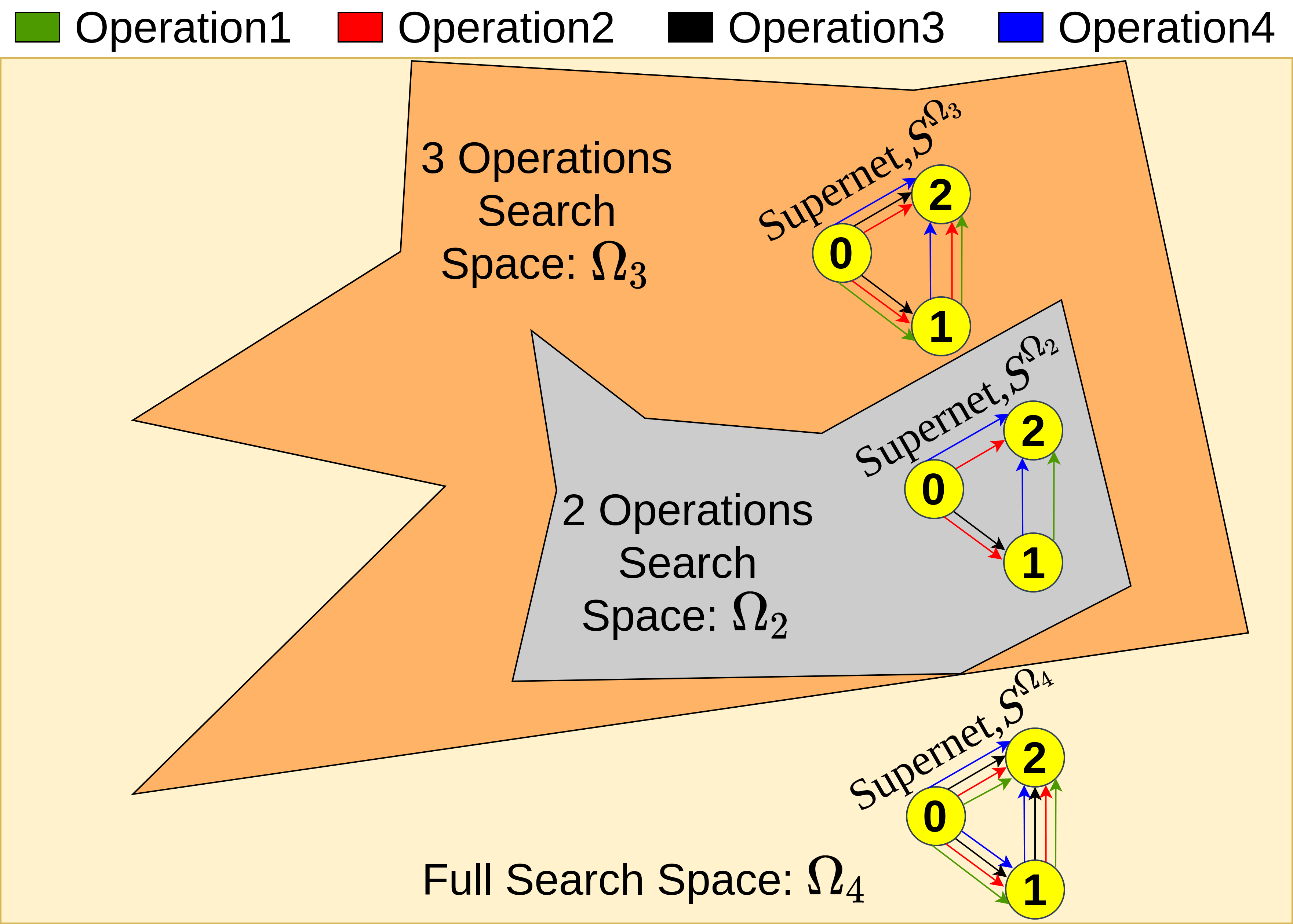
Figure 1: Abstract illustration of progressive reduction of search space along with its corresponding supernet. The search starts from full search space ($\Omega_{4}$) with 4 operations and is then progressively reduced to smaller search space regions: $\Omega_{3},\Omega_{2}$ with 3 and 2 operations respectively. Different colored arrows in supernets are used to represent different operations allowed in a specific search space.

In this paper, we propose a method called pEvoNAS (Neural Architecture Search using Progressive Evolution), which involves progressively reducing the search space by identifying the search space regions with good solution through a genetic algorithm. The fitness/performance of an architecture in any search space is estimated using a supernet which is created using the allowed operations in a particular search space. A supernet represents all possible architectures in the search space while sharing the weights among all the architectures. As illustrated in Figure 1, the architecture search starts from the full search space ($\Omega_{4}$) with 4 operations for 3 nodes and a supernet, $S^{\Omega_{4}}$, is created with the 3 nodes and 4 different colored arrows representing compound edges (i.e. parallel operations) between the nodes. Reducing the search space to $\Omega_{3}$ and $\Omega_{2}$ involves reducing the number of operations between any two nodes to 3 and 2 respectively, which is reflected in their corresponding supernets, ($S^{\Omega_{3}}$, $S^{\Omega_{2}}$). The use of supernet for architecture evaluation results in reduction of search time as compared to vanilla EA-based methods. Also, it can be observed that the supernet for the larger search space (e.g. $S^{\Omega_{3}}$) includes all the operations present in the supernet for the smaller search space (e.g. $S^{\Omega_{2}}$). So, instead of intializing the smaller supernet, e.g. $S^{\Omega_{2}}$, with random weights, it inherits the respective weights from the previous bigger supernet, $S^{\Omega_{3}}$. This is known as supernet weight inheritance.

$\#$ Operations	5	3	2
Kendall Tau	$0.16$	$0.17$	$0.35$

Table 1: Correlation score (Kendall Tau) at different number of operations.

Our contributions can be summarized as follows:

• We designed a framework of progressively reducing the search space to regions in the search space with good solutions using genetic algorithm.

• We also show the effectiveness of the weight inheritance for supernet wherein a supernet for a smaller search space inherits weights from the trained supernet for the bigger search space.

• We also created a visualization of the progressive reduction of search space performed by pEvoNAS to get insights into the search process and show that pEvoNAS indeed reduces the search space to good quality regions in the search space.

2 Motivation

The use of supernet for architecture evaluations results in degraded architecture search performance because of the inaccurate performance estimation by the supernet. This was first reported in [2] and they showed that the co-adaptation among the operations in the compound edge leads to low correlation between the predicted performance via supernet and the true architecture performance from training-from-scratch. In other words, the effect of co-adaptation is due to the combined operations in the compound edge. Following the logic, it seems reasonable that the supernet prediction will improve as number of operations reduce in the compound edge. For example, in Figure 1, the supernet $S^{\Omega_{3}}$ has 3 operations between any two nodes as compared to 2 operations in $S^{\Omega_{2}}$.

We designed a controlled exeriment to test the assumption that as we reduce the number of operations in compound edge, the performance prediction of supernet improves. We use NAS-Bench-201 [9] search space, which has 5 operations in the full search space. First, we train the supernet created using the operations in the full search space for 50 epochs and then compare the supernet predicted architecture performance of all the architectures in the search space with the ground truth provided in NAS-Bench-201. We randomly reduce the number of operations from 5 to 3 operations and create a supernet for the new smaller search space with weights inherited from previous trained supernet. We repeat the training of the new supernet again for 50 epochs and then comparing its prediction. Lastly, we repeat the process again for the new random search space of 2 operations. In Table 1, the correlation coefficient, Kendall’s Tau [14], is used to measure the correlation between estimated accuracy via supernet and ground truth accuracy and found that it increases as we reduce the number of operations considered between any two nodes in the supernet. Based on this observation, we use evolution to find smaller regions with good solutions while using supernet for the architecture evaluation in the search spaces.

3 Related Work

The various NAS methods can be classified into two categories: gradient-based methods and non-gradient based methods.

Gradient-Based Methods: In general, these methods, [20][8] [36][7], relax the discrete architecture search space to a continuous search space by using a supernet. The performance of the supernet on the validation data is used for updating the architecture using gradients. As the supernet shares weights among all architectures in the search space, these methods take lesser time in the evaluation process and thus shorter search time. However, these methods suffer from the overfitting problem wherein the resultant architecture shows good performance on the validation data but exhibits poor performance on the test data. This can be attributed to its preference for parameter-less operations in the search space, as it leads to rapid gradient descent, [3]. In contrast to these gradient-based methods, our method does not suffer from the overfitting problem because of its stochastic nature.

Non-Gradient Based Methods: These methods include reinforcement learning (RL) methods and evolutionary algorithm (EA) methods. In the RL methods [39] [40], an agent is used for the generating neural architecture and the agent is then trained to generate architectures in order to maximize its expected accuracy on the validation data. These accuracies were calculated by training the architectures from scratch to convergence which resulted in long search time. This was improved in [24] by using a single directed acyclic graph (DAG) for sharing the weights among all the sampled architectures, thus resulting in reduced computational resources. The EA based NAS methods begin with a population of architectures and each architecture in the population is evaluated on the basis of its performance on the validation data. The popluation is then evolved on the basis of the performance of the population. Methods such as those proposed in [25] and [35] used gradient descent for optimizing the weights of each architecture in the population from scratch in order to determine their accuracies on the validation data as their fitness, resulting in huge computational requirements. In order to speed up the training process, in [26], the authors introduced weight inheritance wherein the architectures in the new generation population inherit the weights of the previous generation population, resulting in bypassing the training from scratch. However, the speed up gained is less as it still needs to optimize the weights of the architecture. Methods such as that proposed in [31] used a random forest for predicting the performance of the architecture during the evaluation process, resulting in a high speed up as compared to previous EA methods. However, its performance was far from the state-of-the-art results. In contrast, our method achieved better results than previous EA methods while using significantly less computational resources.

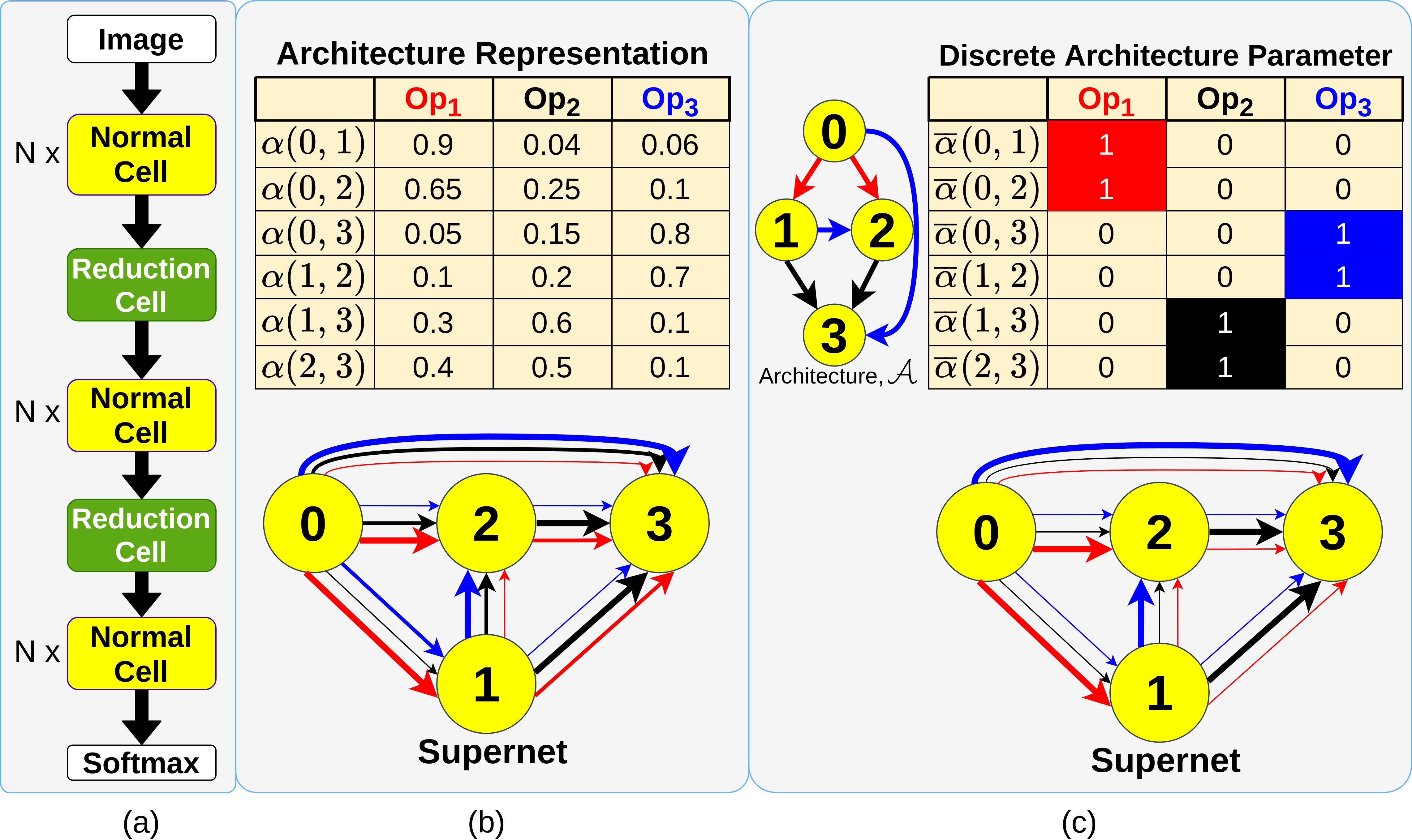
Figure 2: (a) Architecture created by staking cells. (b) Architecture representation for a search space with 3 operations and 4 nodes. The thickness of the arrow in the supernet is proportional to the weight given to an operation. (c) Illustration of selecting an architecture in the supernet. The highlighted cell represents the selected operation between any two nodes.

4 Proposed Method

4.1 Search Space and Architecture Representation

Following [24][25] [40] [20][8][7][23] [18], the architecture is created by staking together cells of two types: normal cells which preserve the dimentionality of the input with a stride of one and reduction cells which reduce the spatial dimension with a stride of two, shown in Figure 2(a). As illustrated in Figure 2(b), a cell in the architecture is represented by an architecture parameter, $\alpha$. Each $\alpha$ for a normal cell and a reduction cell is represented by a matrix with columns representing the weights of different operations $Op(.)s$ from the operation space $\mathcal{O}$ (i.e. the search space of NAS) and rows representing the edge between two nodes. For example, in Figure 2(b), $\alpha(0,1)$ represents the edge between node 0 and node 1 and the entries in the row represent the weights given to the three different operations.

4.2 Performance Estimation

We used a supernet [20] to estimate the performance of an architecture in the search space. It shares the weights among all architectures in the search space by treating all the architectures as the subgraphs of a supergraph. As illustrated in Figure 2(b), the supernet uses the architecture parameter, $\alpha$, by normalizing it using softmax. The directed edge from node $i$ to node $j$ is the weighted sum of all $Op(.)s$ in $\mathcal{O}$ where the $Op(.)s$ are weighted by the normalized $\alpha^{(i,j)}$. This can be written as:

$$f^{(i,j)}(x^{(i)})=\sum_{Op\in\mathcal{O}}\frac{exp(\alpha^{(i,j)}_{Op})}{\sum_{Op^{\prime}\in\mathcal{O}}exp(\alpha^{(i,j)}_{Op^{\prime}})}Op(x^{(i)})$$ (1)

where $\alpha^{(i,j)}_{op}$ represents the weight of the operation $Op(.)$ in the operation space $\mathcal{O}$ between node $i$ and node $j$. This design choice allows us to skip the individual architecture training from scratch for its evaluation because of the weight-sharing nature of the supernet, thus resulting in a significant reduction of search time. The supernet is trained on training dataset for a certain number of epochs using Stochastic Gradient Descent (SGD), [34] with momentum. During training, random architecture parameter, $\alpha$, is sent to the supernet for each training batch in an epoch so that no particular sub-graph (i.e. architecture) of the super-graph (i.e. supernet) receives most of the gradient updates.

The performance of an architecture is calculated using the trained supernet on the validation data, also known as the fitness of the architecture. As illustrated in Figure 2(c), in order to select an architecture, $\mathcal{A}$, in the supernet, a new architecture parameter called discrete architecture parameter, $\bar{\alpha}$ is created with the following entries:

$$\bar{\alpha}^{(i,j)}_{Op}=\begin{cases}1,\text{if $Op(x^{(i)})$ present in $A$}\\ 0,\text{otherwise}\\ \end{cases}$$ (2)

Using $\bar{\alpha}$, the architecture, $A$, is selected in the supernet and the accuracy of the supernet on the validation data is used as the estimated fitness of $A$.

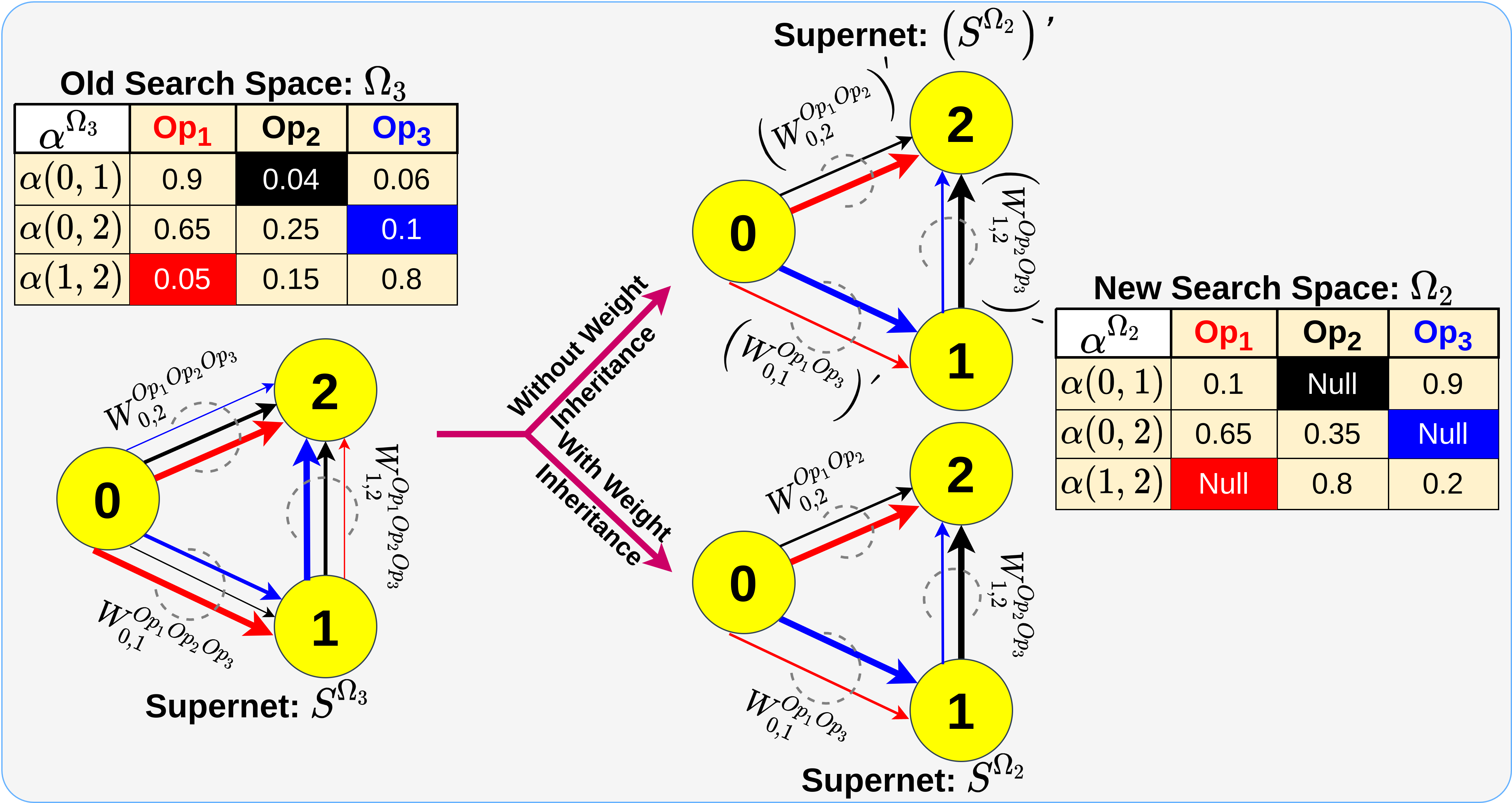
Figure 3: Abstract illustration of reduction of search space from a bigger search space with 3 operations to smaller search space with 2 operations. The highlighted cells are the operations that have been removed from the search space. $W_{n_{1},n_{2}}^{Op(.)}$ represents the weights of the allowed operations between node $n_{1}$ and node $n_{2}$. $(W_{n_{1},n_{2}}^{Op(.)})^{\prime}$ represents randomly initialized weights.

4.3 Search Space Reduction

Reducing the search space involves reducing the number of operations considered between any two nodes. This is done by selecting the top-k operations in each row of the $\alpha$ where k represents the number of operations for the new reduced search space. For example, in Figure 3, the top-2 operations ($Op_{2},Op_{3}$) are selected in $\alpha(1,2)$ from the old search space, $\Omega_{3}$, to create a new search space $\Omega_{2}$. Since all the operations present in $\Omega_{2}$ are also present in $\Omega_{3}$, the supernet for $\Omega_{2}$, (i.e. $S^{\Omega_{2}}$), can be created in 2 ways: (i) With Supernet Weight Inheritance: Here, the smaller search space supernet inherits/copies the weights from the previous bigger search space supernet. (ii) Without Supernet Weight Inheritance: Here, the smaller search space supernet is created with random weights. For example, in Figure 3, the weights of the operations between node 1 and 2 for $S^{\Omega_{2}}$ are inherited from $S^{\Omega_{3}}$ while the weights of the operations in $(S^{\Omega_{2}})^{\prime}$ are randomly intialized.

Input: Population size $N_{pop}$, training data $\mathfrak{D}_{tr}$, validation data $\mathfrak{D}_{va}$, training epochs $N_{epochs}$, list of operation numbers $\mathfrak{Op}$, convergence number $N_{conv}$.

Output: Best architecture, $E_{best}$.

1 foreach  $op\in\mathfrak{Op}$ do

2      if smaller search space then

             /* Search space reduction */

3             Reduce search space to $op$ operations, $\Omega_{op}$, using $E_{best}$;

             /* Weight inheritance */

4             Create supernet, $S^{\Omega_{op}}$, with weights $W$ inherited from previous supernet;

5            

6       else // For full search space

7             Initialize supernet, $S^{\Omega_{op}}$, with random weights $W$ for full search space;

8            

9       end if

10      

11      TrainSupernet($S^{\Omega_{op}}$,$N_{epochs}$, $\mathfrak{D}_{tr}$);

12      

      /* Architecture search using evolution */

13       $E_{best}\leftarrow$ EA($\Omega_{op}$, $S^{\Omega_{op}}$, $N_{conv}$, $\mathfrak{D}_{va}$, $N_{pop}$);

14       if Final search space then

15             return $E_{best}$

16       end if

17      

18 end foreach

Algorithm 1 pEvoNAS

4.4 pEvoNAS

The entire process is summarized in Algorithm 1. It begins with a list of number of operations, $\mathfrak{Op}$, to which the search space is to be reduced. For each operation number, $op\in\mathfrak{Op}$, a supernet, $S^{\Omega_{op}}$, is created for the search space, $\Omega_{op}$. If it is the first search space (i.e. full search space) then the weights of $S^{\Omega_{op}}$ are randomly initialized, otherwise they are inherited from the previous search space trained supernet. The supernet, $S^{\Omega_{op}}$, is then trained for $N_{epochs}$ epochs. The evolutionary algorithm (EA) then performs the architecture search in $\Omega_{op}$. It starts with a population of $N_{pop}$ architectures, which are sampled from a uniform distribution on the interval $\left[0,1\right)$. Fitness of each individual in the population is evaluated using the trained $S^{\Omega_{op}}$. The population is then evolved using crossover and mutation operations to create the next generation population replacing the previous generation population. The best architecture, $E_{best}$, in each generation does not undergo any modification and is automatically copied to the next generation. This ensures that the algorithm does not forget the best architecture learned thus far and gives an opportunity to old generation architecture to compete against the new generation architecture. The process of population evaluation and then evolution is repeated until $E_{best}$ does not change for $N_{conv}$ generations, showing the convergence to an architecture. $E_{best}$ is then used to reduce the reduce the search space. The whole process is repeated until the search space is reduced to the final search space, $\Omega_{final}$. For $\Omega_{final}$, $E_{best}$ is returned as the searched architecture. The pseudocodes for the supernet training and the evolutionary algorithm are given in the supplementary.

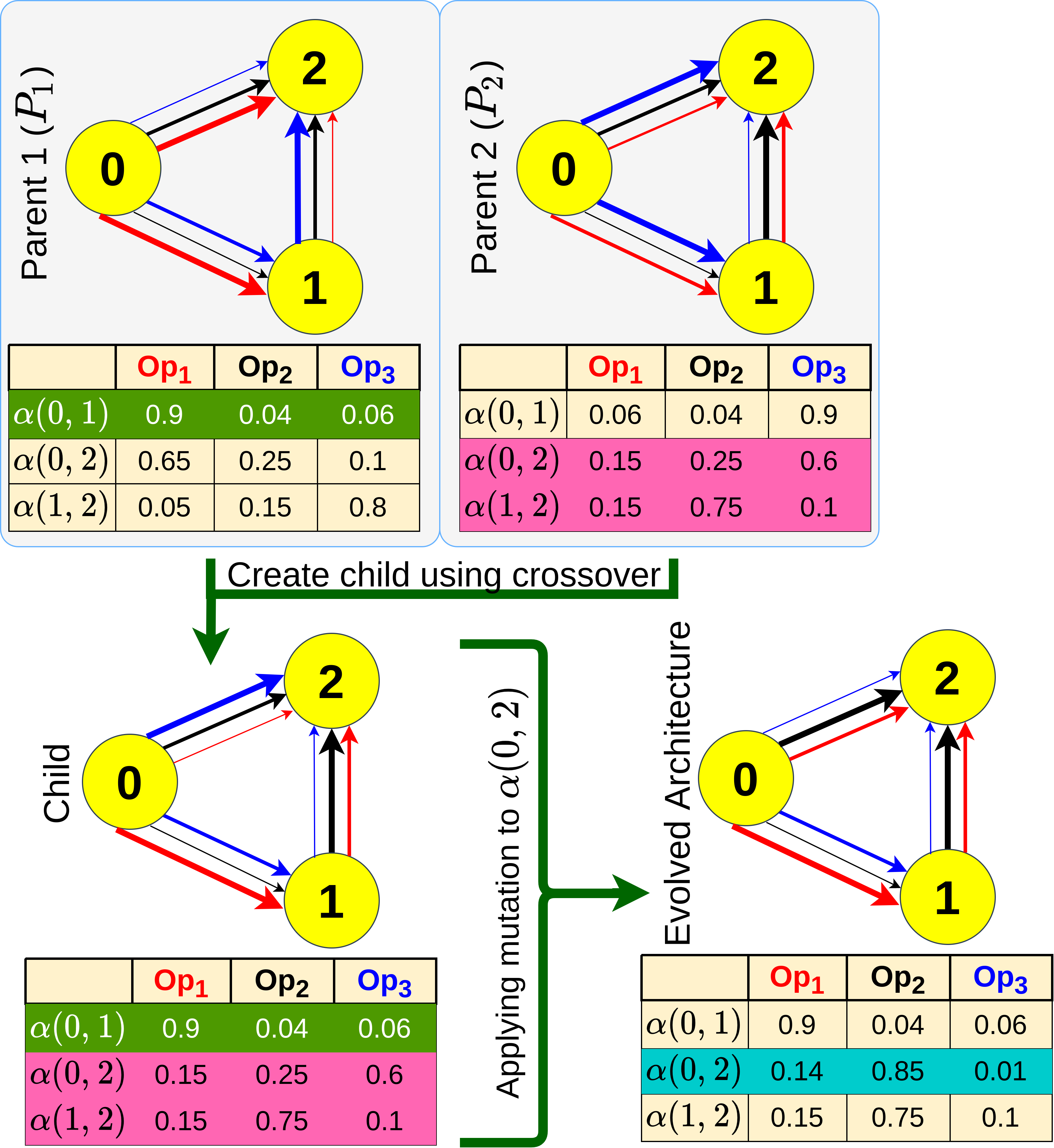
Figure 4: Abstract illustration of the evolution process using crossover and mutation.

Crossover and Mutation Operations: Crossover combines 2 parents ($P_{1}$, $P_{2}$), selected through tournament selection [10], to create a new child architecture, which may perform better than the parents. In tournament selection, a certain number of architectures are randomly selected from the current population and the most fit architecture from the selected group becomes the parent. We get $P_{1}$ and $P_{1}$ on applying tournament selection two times which are then used to create a single child architecture. This is done by copying the edge between $node_{i}$ and $node_{j}$, from either $P_{1}$ or $P_{2}$, with 50% probability, to the child architecture between $node_{i}$ and $node_{j}$. Mutation refers to a random change to an individual architecture in the population. The algorithm uses the mutation rate [10], which decides the probability of changing the architecture parameter, $\alpha^{i,j}$, between node $i$ and node $j$. This is done by re-sampling $\alpha^{i,j}$ from a uniform distribution on the interval $\left[0,1\right)$. As illustrated in Figure  4, ${\alpha}^{0,1}_{child}$ and ${\alpha}^{1,2}_{child}$ are copied from $P_{1}$ and $P_{2}$ respectively during crossover while applying mutation to ${\alpha}^{0,2}_{child}$ in the child architecture.

5 Experiments

5.1 Search Spaces

In this section, we report the performance of progEvoNAS in terms of a neural architecture search on two different search spaces: 1) Search space 1 (S1) [20] and 2) Search space 2 (S2)[9]. In S1, we search for both normal and reduction cells where each node $x^{(j)}$ maps two inputs to one output. Here, each cell has seven nodes with first two nodes being the output from previous cells and last node as output node, resulting in 14 edges among them. There are 8 operation in S1, so each architecture is represented by two 14x8 matrices, one each for normal cell and reduction cell. In S2, we search for only normal cells, where each node $x^{(j)}$ is connected to the previous node $x^{(i)}$ (i.e. $i<j$). It is a smaller search space where we only search for the normal cell in Figure 2(a). It provides a unified benchmark for almost any up-to-date NAS algorithm by providing results of each architecture in the search space on CIFAR-10, CIFAR-100 and ImageNet-16-12. Here, each cell has four nodes with first node as input node and last node as output node, resulting in 6 edges among them. There are 5 operations in S2, so each architecture is represented by one 6x5 matrix for the normal cell.

5.2 Dataset

CIFAR-10 and CIFAR-100 [15] has 50K training images and 10K testing images with images classified into 10 classes and 100 classes respectively. ImageNet [5] is well known benchmark for image classification containing 1K classes with 1.28 million training images and 50K images test images. ImageNet-16-120 [4] is a down-sampled variant of ImageNet where the original ImageNet is downsampled to 16x16 pixels with labels $\in\left[0,120\right]$ to construct ImageNet-16-120 dataset. The settings used for the datasets in S1 are as follows:

• CIFAR-10: We split 50K training images into two sets of size 25K each, with one set acting as the training set and the other set as the validation set.

• CIFAR-100: We split 50K training images into two sets. One set of size 40K images becomes the training set and the other set of size 10K images becomes the validation set.

The settings used for the datasets in S2 are as follows:

• CIFAR-10: The same settings as those used for S1 is used here as well.

• CIFAR-100: The 50K training images remains as the training set and the 10K testing images are split into two sets of size 5K each, with one set acting as the validation set and the other set as the test set.

• ImageNet-16-120: It has 151.7K training images, 3K validation images and 3K test images.

5.3 Implementation Details

5.3.1 Supernet Training Settings:

In general, the supernet suffers from high memory requirements which makes it difficult to fit it in a single GPU. For S1, we follow [20] and use a smaller supernet, called proxy model which is created with 20 stacked cells and 16 initial channels. It is trained on both CIFAR-10 and CIFAR-100 with SGD for 50 epochs (i.e. $N_{epochs}$), which is chosen based on the experiment conducted in S2, shown in Figure 5(a). All the other settings are also same for both datasets i.e. batch size of 64, weight decay $\lambda=3\times 10^{-4}$, cutout[6], initial learning rate $\eta_{max}=0.025$ (annealed down to 0 by using a cosine schedule without restart[21]) and momentum $\rho=0.9$. For S2, we do not use a proxy model as the size of the supernet is sufficiently small to be fitted in a single GPU. For training, we follow the same settings as those used in S1 for CIFAR-10, CIFAR-100 and ImageNet16-120 except batch size of 256.

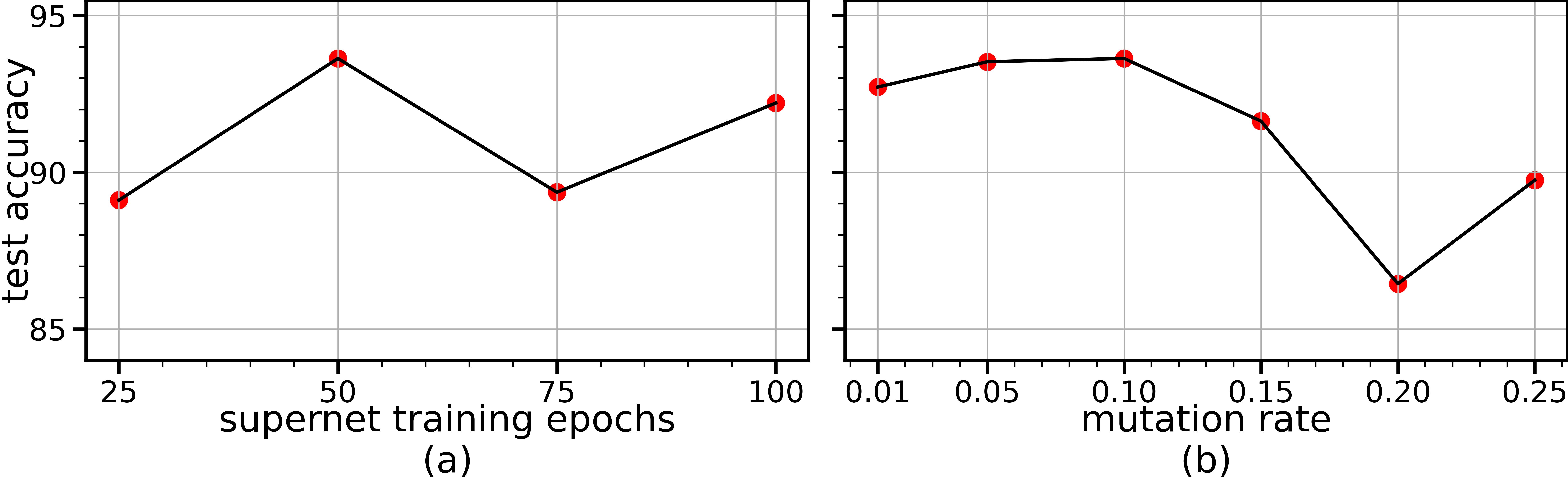
Figure 5: Tests conducted for hyperparameter selection in S2. Test accuracy vs (a) training epochs of supernet, and (b) mutation rate.

5.3.2 Architecture evaluation:

Here, the discovered architecture, $E_{best}$ (i.e. discovered cells), at the end of the architecture search is trained on the dataset to evaluate its performance for comparing with other NAS methods. For S1, we follow the training settings used in DARTS [20]. Here, a larger network, called proxyless network [17], is created using $E_{best}$ with 20 stacked cells and 36 initial channels for both CIFAR-10 and CIFAR-100 datasets. It is then trained for 600 epochs on both the datasets with the same settings as the ones used in the supernet training above. Following recent works [24][25][40] [20][18], we use an auxiliary tower with 0.4 as its weights, path dropout probability of 0.2 and cutout [6] for additional enhancements. For ImageNet, $E_{best}$ is created with 14 cells and 48 initial channels in the mobile setting, wherein the input image size is 224 x 224 and the number of multiply-add operations in the model is restricted to less than 600M. It is trained on 8 NVIDIA V100 GPUs by following the training settings used in [3].

Table 2: Comparison of pEvoNAS with other NAS methods in S1 in terms of test accuracy (higher is better) on CIFAR-10.

Architecture	Top-1	Params	GPU	Search
	Acc. (%)	(M)	Days	Method
ResNet[12]	95.39	1.7	-	manual
DenseNet-BC[13]	96.54	25.6	-	manual
ShuffleNet[38]	90.87	1.06	-	manual
PNAS[18]	96.59	3.2	225	SMBO
RSPS[17]	97.14	4.3	2.7	random
NASNet-A[40]	97.35	3.3	1800	RL
ENAS[24]	97.14	4.6	0.45	RL
DARTS[20]	97.24	3.3	4	gradient
GDAS[8]	97.07	3.4	0.83	gradient
SNAS[36]	97.15	2.8	1.5	gradient
SETN[7]	97.31	4.6	1.8	gradient
AmoebaNet-A[25]	96.66	3.2	3150	EA
Large-scale Evo.[26]	94.60	5.4	2750	EA
Hierarchical Evo.[19]	96.25	15.7	300	EA
CNN-GA[33]	96.78	2.9	35	EA
CGP-CNN[30]	94.02	1.7	27	EA
AE-CNN[32]	95.7	2.0	27	EA
NSGANetV1-A2[23]	97.35	0.9	27	EA
AE-CNN+E2EPP[31]	94.70	4.3	7	EA
NSGA-NET[22]	97.25	3.3	4	EA
pEvoNAS-C10A	97.52	3.6	1.20	EA
pEvoNAS-C10B	97.36	3.5	1.31	EA
pEvoNAS-C10C	97.27	3.0	1.41	EA
pEvoNAS-C10rand	96.83	3.37	0.11	random

Table 3: Comparison of pEvoNAS with other NAS methods in S1 in terms of test accuracy (higher is better) on CIFAR-100.

Architecture	Top-1	Params	GPU	Search
	Acc. (%)	(M)	Days	Method
ResNet[12]	77.90	1.7	-	manual
DenseNet-BC[13]	82.82	25.6	-	manual
ShuffleNet[38]	77.14	1.06	-	manual
PNAS[18]	80.47	3.2	225	SMBO
MetaQNN[1]	72.86	11.2	90	RL
ENAS[24]	80.57	4.6	0.45	RL
AmoebaNet-A[25]	81.07	3.2	3150	EA
Large-scale Evo.[26]	77.00	40.4	2750	EA
CNN-GA[33]	79.47	4.1	40	EA
AE-CNN[32]	79.15	5.4	36	EA
NSGANetV1-A2[23]	82.58	0.9	27	EA
Genetic CNN[35]	70.95	-	17	EA
AE-CNN+E2EPP[31]	77.98	20.9	10	EA
NSGA-NET[22]	79.26	3.3	8	EA
pEvoNAS-C100A	82.59	3.0	1.25	EA
pEvoNAS-C100B	82.44	3.1	1.28	EA
pEvoNAS-C100C	82.23	3.3	1.22	EA
pEvoNAS-C100rand	81.03	2.8	0.15	random

Table 4: Comparison of pEvoNAS with other NAS methods in S1 in terms of test accuracy (higher is better) on ImageNet.

Architecture	Test Accuracy (%)		Params	+$\times$	GPU	Search
	top 1	top 5	(M)	(M)	Days	Method
MobileNet-V2, ([27])	72.0	91.0	3.4	300	-	manual
PNAS, ([18])	74.2	91.9	5.1	588	225	SMBO
NASNet-A, ([40])	74.0	91.6	5.3	564	1800	RL
NASNet-B, ([40])	72.8	91.3	5.3	488	1800	RL
NASNet-C, ([40])	72.5	91.0	4.9	558	1800	RL
DARTS, ([20])	73.3	91.3	4.7	574	4	gradient
GDAS, ([8])	74.0	91.5	5.3	581	0.83	gradient
SNAS, ([36])	72.7	90.8	4.3	522	1.5	gradient
SETN, ([7])	74.3	92.0	5.4	599	1.8	gradient
AmoebaNet-A, ([25])	74.5	92.0	5.1	555	3150	EA
AmoebaNet-B, ([25])	74.0	91.5	5.3	555	3150	EA
AmoebaNet-C, ([25])	75.7	92.4	6.4	570	3150	EA
NSGANetV1-A2, ([23])	74.5	92.0	4.1	466	27	EA
pEvoNAS-C10A	74.9	92.4	5.1	567	1.20	EA
pEvoNAS-C100A	73.2	91.3	4.3	478	1.25	EA

5.3.3 Evolutionary Algorithm Settings:

The architecture search begins with the full search space for both the search spaces. So, for S1, the architecture search begins with the search space with 8 operations which is then progressively reduced to smaller search space regions with 5 operations and then finally to 2 operations. While, for S2, the architecture search begins with the search space with 5 operations which is then progressively reduced to search spaces with 3 and 2 operations. Following [31][32], the evolutionary algorithm (EA), for both S1 and S2, uses a population size of 20 in each generation. For the tournament selection, 5 architectures are chosen randomly from the current population and the best best architecture among them becomes the parent. We apply the tournament selection 2 times to get 2 parents for the crossover operation. Mutation rate of 0.1 was chosen based on the experiment conducted in S2, shown in Figure 5(b). The evolutionary search runs until the best architecture, $E_{best}$, is repeated for 10 generations (i.e. $N_{conv}$). All the above training and architecture search were performed on a single Nvidia RTX 3090 GPU.

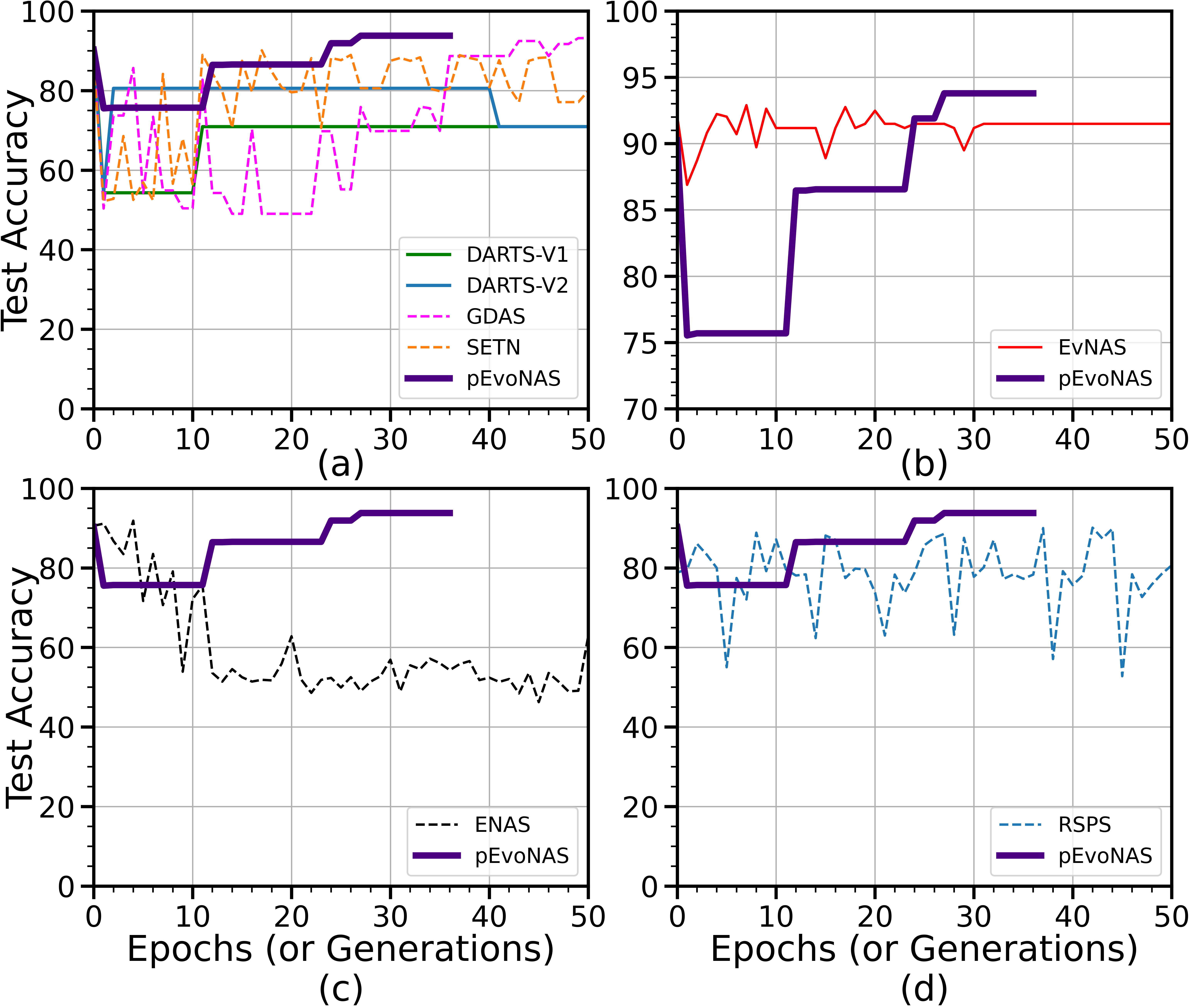
Figure 6: Comparision of pEvoNAS with (a) gradient-based methods, (b) EA-based method, (c) RL method and (d) random search on CIFAR-10 for the search space S2.

Table 5: Comparison of pEvoNAS with other NAS methods on NAS-Bench-201 (i.e. S2)[9] with mean $\pm$ std. accuracies on CIFAR-10, CIFAR-100 and ImageNet16-120 (higher is better). Optimal refers to the best architecture accuracy for each dataset. Search times are given for a CIFAR-10 search on a single GPU.

Method	Search	CIFAR-10		CIFAR-100		ImageNet-16-120		Search
	(seconds)	validation	test	validation	test	validation	test	Method
RSPS [17]	$7587$	$84.16\pm 1.69$	$87.66\pm 1.69$	$59.00\pm 4.60$	$58.33\pm 4.64$	$31.56\pm 3.28$	$31.14\pm 3.88$	random
DARTS-V1 [20]	$10890$	$39.77\pm 0.00$	$54.30\pm 0.00$	$15.03\pm 0.00$	$15.61\pm 0.00$	$16.43\pm 0.00$	$16.32\pm 0.00$	gradient
DARTS-V2 [20]	$29902$	$39.77\pm 0.00$	$54.30\pm 0.00$	$15.03\pm 0.00$	$15.61\pm 0.00$	$16.43\pm 0.00$	$16.32\pm 0.00$	gradient
GDAS [8]	$28926$	$90.00\pm 0.21$	$93.51\pm 0.13$	$71.14\pm 0.27$	$70.61\pm 0.26$	$41.70\pm 1.26$	$41.84\pm 0.90$	gradient
SETN [7]	$31010$	$82.25\pm 5.17$	$86.19\pm 4.63$	$56.86\pm 7.59$	$56.87\pm 7.77$	$32.54\pm 3.63$	$31.90\pm 4.07$	gradient
ENAS [24]	$13314$	$39.77\pm$0.00	$54.30\pm 0.00$	$15.03\pm 00$	$15.61\pm 0.00$	$16.43\pm 0.00$	$16.32\pm 0.00$	RL
EvNAS [29]	22445	88.98$\pm$1.40	92.18$\pm$1.11	66.35$\pm$2.59	66.74$\pm$3.08	39.61$\pm$0.72	39.00$\pm$0.44	EA
pEvoNAS	4509	90.54$\pm$0.57	93.63$\pm$0.42	69.28$\pm$2.13	69.05$\pm$1.99	40.00$\pm$3.22	39.98$\pm$3.76	EA
pEvoNAS (w/o inherit)	4509	86.86$\pm$2.50	89.83$\pm$3.16	67.90$\pm$2.09	68.21$\pm$2.48	36.70$\pm$6.60	35.91$\pm$7.92	EA
ResNet	N/A	$90.83$	$93.97$	$70.42$	$70.86$	$44.53$	$43.63$	manual
Optimal	N/A	$91.61$	$94.37$	$73.49$	$73.51$	$46.77$	$47.31$	N/A

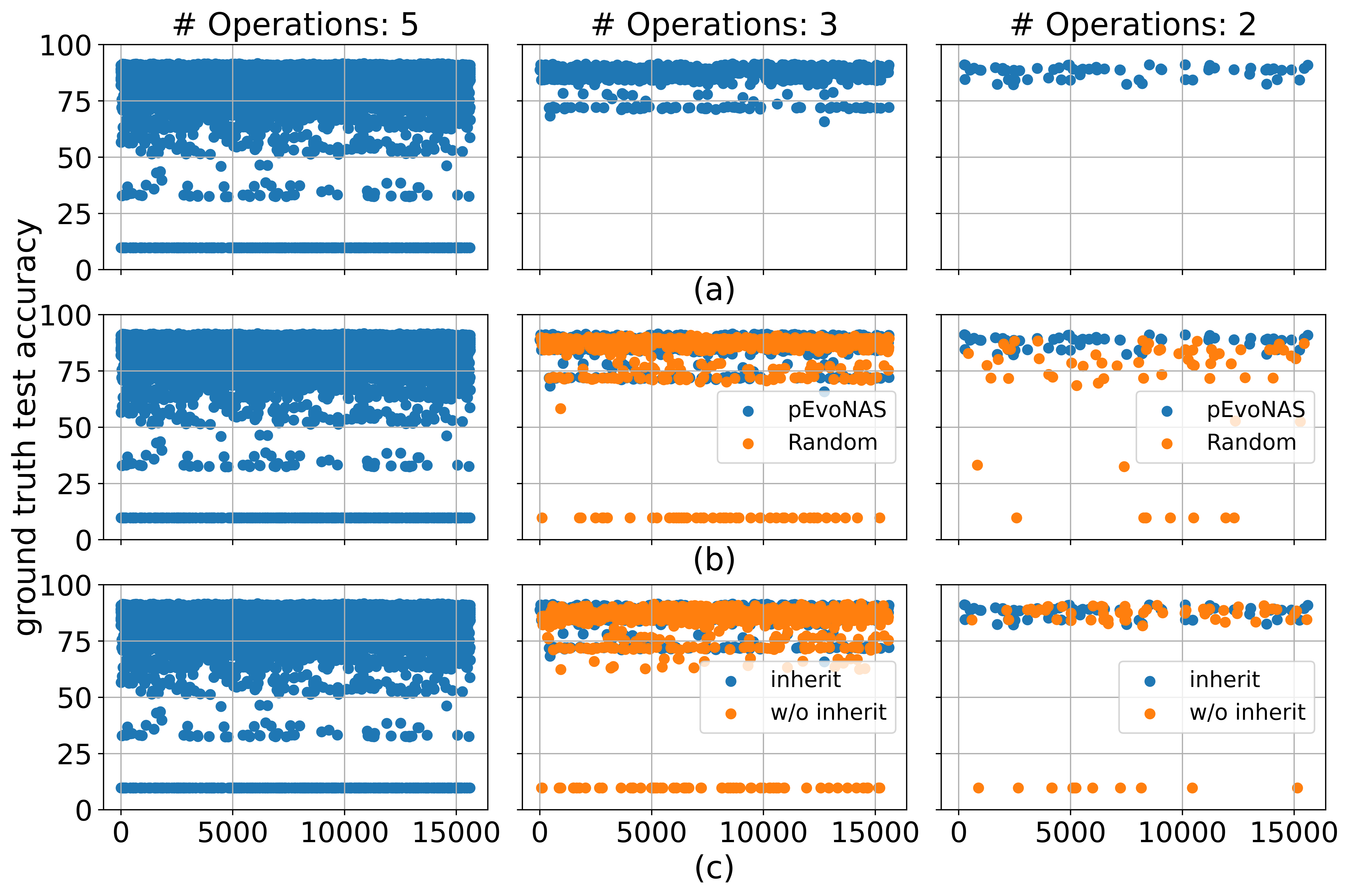
Figure 7: Visualizing the search space by plotting the ground truth accuracies of all architectures in the search space. The x-axis represents all 15,625 architectures in the search space S2 [9] and the y-axis represents the true test accuracies. (a) Search space reduction using pEvoNAS. (b) Comparison of search space reduction using pEvoNAS and random search. (c) Comparison of search space reduction using pEvoNAS with weight inheritance (inherit) and no weight inheritance (w/o inherit).

5.4 Results

5.4.1 Search Space 1 (S1):

We performed 3 architecture searches on both CIFAR-10 and CIFAR-100 with different random number seeds; their results are provided in Table 2 and Table 3. The results show that the cells discovered by pEvoNAS on CIFAR-10 and CIFAR-100 achieve better results than those by human designed, RL based, gradient-based and EA-based methods. On comparing the computation time (or search cost) measured in terms of GPU days, we found that pEvoNAS performs the architecture search in significantly less time as compared to other EA-based methods while giving better search results. GPU days for any NAS method is calculated by multiplying the number of GPUs used in the NAS method by the execution time (reported in units of days). All the discovered architectures for S1 are provided in the supplementary.

We followed [18][20][24] [25][40] to compare the transfer capability of pEvoNAS with that of the other NAS methods, wherein the discovered architecture on a dataset was transferred to another dataset (i.e. ImageNet) by retraining the architecture from scratch on the new dataset. The best discovered architectures from the architecture search on CIFAR-10 and CIFAR-100 (i.e. pEvoNAS-C10A and pEvoNAS-C100A) were then evaluated on the ImageNet dataset in mobile setting and the results are provided in Table 4. The results show that the cells discovered by pEvoNAS on CIFAR-10 and CIFAR-100 can be successfully transferred to ImageNet, while using significantly less computational resources than EA based methods

5.4.2 Search Space 2 (S2):

We performed 3 architecture searches each on CIFAR-10, CIFAR-100 and ImageNet-16-120 and their results are provided in Table 5. The results show that pEvoNAS outperforms most of the NAS methods except GDAS [8] on CIFAR-100 and ImageNet-16-120. However, GDAS performs worse when the size of the search space increases as can be seen for S1 in Table 2. In Figure 6, we compare the progression of the search of pEvoNAS with that of other NAS methods. From the figure, we find that gradient-based method like DARTS, [20], suffers from overfitting problem wherein it converges to parameter-less operation, skip-connect (i.e. a local optimum) [3][37] [9]. In contrast, pEvoNAS does not get stuck to a local optimum architecture due to its stochastic nature. We also find that pEvoNAS converges to a solution much faster than other NAS methods.

6 Futher Analysis

6.1 Visualizing the Architecture Search

For analyzing the architecture search, we use S2 [9] to visualize the search process as it provides the true test accuracies of all the architectures in the search space. As illustrated in Figure 7(a), the search process is visualized by plotting all the architecures present in a given search space. From the figure, we find that the architecture search begins with the full search space (i.e. 5 operations) and is then progressively reduced to smaller search spaces (i.e. 3 operations and 2 Operations). More specifically, pEvoNAS reduces the search spaces to regions with high quality architectures and finally leading to the final search space (i.e. 2 operations) containing all architectures with top test accuracies.

6.2 Ablation Studies

6.2.1 Comparison with Random Search:

Here, the search space, S1, is randomly reduced to the final search space (i.e. # Operation: 2), $\Omega_{2}^{rand}$, and then a trained supernet is used to evaluated 100 random architectures in $\Omega_{2}^{rand}$. The best architecture is then returned as the final architecture, reported in Table 2 and Table 3 as pEvoNAS-C10rand and pEvoNAS-C100rand for CIFAR-10 and CIFAR-100 respectively. We found that the random search performs worse than pEvoNAS while taking lesser search time. To analyze the random search, we visualize the search space discovered using the random search in S2, shown in Figure 7(b), by randomly reducing the search space to smaller search spaces (i.e. 3 operations and 2 Operations). From the figure, we can see that the random search space reduction selects the search space with both good and bad quality architectures which results into degraded output architecture.

6.2.2 Effectiveness of Weight Inheritance:

To illustrate the effectiveness of the weight inheritance of supernet, we perform the architecture search without weight inheritance in the search space S2 (given in Table 5) and found degraded search performance on all 3 datasets. We further analyze the differences in the search processes by plotting the search spaces discovered by pEvoNAS with inheritance and without inheritance respectively in Figure 7(c). From the figure, we see that the final search space discovered by not using weight inheritance contains both low and high quality architectures as compared to only high quality architectures for pEvoNAS with weight inheritance. This reduction to lower quality search space shows the effectiveness of the weight inheritance of supernet during the search process.

7 Conclusion

The goal of this paper was to mitigate the noisy fitness estimation nature of the supernet by progressively reducing the search space to smaller regions of good quality architecture. This was achieved by using a trained supernet for architecture evaluation during the architecture search while using genetic algorithm to find regions in the search space with good quality architectures. The search then progressively reduces the search space to these regions and continues to search using a smaller supernet which inherits its weights from previous supernet. The use of trained supernet for evaluating the architectures in the population allowed us to skip the training of each individual architecture from sratch for its fitness evaluation and thus resulting in the reduced search time. We applied pEvoNAS to two different search spaces to show its effectiveness in generalizing to any cell-based search space. Experimentally, pEvoNAS reduced the search time of EA-based search methods significantly while achieving better results on CIFAR-10 and CIFAR-100 datasets in S1 search space. We also visualized the search process using the NAS benchmark, NAS-Bench-201[9] and found that pEvoNAS progressively reduces the search space to smaller search spaces with top accuracy architectures.

References

- [1] Bowen Baker, Otkrist Gupta, Nikhil Naik, and Ramesh Raskar. Designing neural network architectures using reinforcement learning. International Conference on Learning Representations, 2017.
- [2] Gabriel Bender, Pieter-Jan Kindermans, Barret Zoph, Vijay Vasudevan, and Quoc Le. Understanding and simplifying one-shot architecture search. In International Conference on Machine Learning, pages 550–559. PMLR, 2018.
- [3] Xin Chen, Lingxi Xie, Jun Wu, and Qi Tian. Progressive differentiable architecture search: Bridging the depth gap between search and evaluation. In Proceedings of the IEEE International Conference on Computer Vision, pages 1294–1303, 2019.
- [4] Patryk Chrabaszcz, Ilya Loshchilov, and Frank Hutter. A downsampled variant of imagenet as an alternative to the cifar datasets. arXiv preprint arXiv:1707.08819, 2017.
- [5] J. Deng, W. Dong, R. Socher, L. Li, Kai Li, and Fei-Fei Li. Imagenet: a large-scale hierarchical image database. In 2009 IEEE Conference on Computer Vision and Pattern Recognition, pages 248–255, 2009.
- [6] Terrance DeVries and Graham W Taylor. Improved regularization of convolutional neural networks with cutout. arXiv preprint arXiv:1708.04552, 2017.
- [7] Xuanyi Dong and Yi Yang. One-shot neural architecture search via self-evaluated template network. In Proceedings of the IEEE International Conference on Computer Vision, pages 3681–3690, 2019.
- [8] Xuanyi Dong and Yi Yang. Searching for a robust neural architecture in four gpu hours. In Proceedings of the IEEE Conference on computer vision and pattern recognition, pages 1761–1770, 2019.
- [9] Xuanyi Dong and Yi Yang. Nas-bench-201: Extending the scope of reproducible neural architecture search. In International Conference on Learning Representations, 2020.
- [10] Agoston E Eiben, James E Smith, et al. Introduction to evolutionary computing, volume 53. Springer, 2003.
- [11] Thomas Elsken, Jan Hendrik Metzen, and Frank Hutter. Neural architecture search: A survey. arXiv preprint arXiv:1808.05377, 2018.
- [12] Kaiming He, Xiangyu Zhang, Shaoqing Ren, and Jian Sun. Deep residual learning for image recognition. In Proceedings of the IEEE Conference on Computer Vision and Pattern Recognition, pages 770–778, 2016.
- [13] Gao Huang, Zhuang Liu, Laurens Van Der Maaten, and Kilian Q Weinberger. Densely connected convolutional networks. In Proceedings of the IEEE Conference on Computer Vision and Pattern Recognition, pages 4700–4708, 2017.
- [14] Maurice G Kendall. A new measure of rank correlation. Biometrika, 30(1/2):81–93, 1938.
- [15] Alex Krizhevsky, Geoffrey Hinton, et al. Learning multiple layers of features from tiny images. 2009.
- [16] Alex Krizhevsky, Ilya Sutskever, and Geoffrey E Hinton. Imagenet classification with deep convolutional neural networks. In Advances in Neural Information Processing Systems, pages 1097–1105, 2012.
- [17] Liam Li and Ameet Talwalkar. Random search and reproducibility for neural architecture search. In Uncertainty in Artificial Intelligence, pages 367–377. PMLR, 2020.
- [18] Chenxi Liu, Barret Zoph, Maxim Neumann, Jonathon Shlens, Wei Hua, Li-Jia Li, Fei-Fei Li, Alan Yuille, Jonathan Huang, and Kevin Murphy. Progressive neural architecture search. In Proceedings of the European Conference on Computer Vision (ECCV), pages 19–34, 2018.
- [19] Hanxiao Liu, Karen Simonyan, Oriol Vinyals, Chrisantha Fernando, and Koray Kavukcuoglu. Hierarchical representations for efficient architecture search. In International Conference on Learning Representations, 2018.
- [20] Hanxiao Liu, Karen Simonyan, and Yiming Yang. DARTS: Differentiable architecture search. In International Conference on Learning Representations, 2019.
- [21] Ilya Loshchilov and Frank Hutter. SGDR: stochastic gradient descent with warm restarts. In 5th International Conference on Learning Representations, ICLR 2017, Toulon, France, April 24-26, 2017, Conference Track Proceedings. OpenReview.net, 2017.
- [22] Zhichao Lu, Ian Whalen, Vishnu Boddeti, Yashesh Dhebar, Kalyanmoy Deb, Erik Goodman, and Wolfgang Banzhaf. Nsga-net: neural architecture search using multi-objective genetic algorithm. In Proceedings of the Genetic and Evolutionary Computation Conference, pages 419–427, 2019.
- [23] Zhichao Lu, Ian Whalen, Yashesh Dhebar, Kalyanmoy Deb, Erik Goodman, Wolfgang Banzhaf, and Vishnu Naresh Boddeti. Multi-objective evolutionary design of deep convolutional neural networks for image classification. IEEE Transactions on Evolutionary Computation, 2020.
- [24] Hieu Pham, Melody Guan, Barret Zoph, Quoc Le, and Jeff Dean. Efficient neural architecture search via parameters sharing. In Jennifer Dy and Andreas Krause, editors, Proceedings of the 35th International Conference on Machine Learning, volume 80 of Proceedings of Machine Learning Research, pages 4095–4104, Stockholmsmässan, Stockholm Sweden, 10–15 Jul 2018. PMLR.
- [25] Esteban Real, Alok Aggarwal, Yanping Huang, and Quoc V Le. Regularized evolution for image classifier architecture search. In Proceedings of the AAAI Conference on Artificial Intelligence, volume 33, pages 4780–4789, 2019.
- [26] Esteban Real, Sherry Moore, Andrew Selle, Saurabh Saxena, Yutaka Leon Suematsu, Jie Tan, Quoc V Le, and Alexey Kurakin. Large-scale evolution of image classifiers. In Proceedings of the 34th International Conference on Machine Learning-Volume 70, pages 2902–2911. JMLR. org, 2017.
- [27] Mark Sandler, Andrew Howard, Menglong Zhu, Andrey Zhmoginov, and Liang-Chieh Chen. Mobilenetv2: Inverted residuals and linear bottlenecks. In Proceedings of the IEEE conference on computer vision and pattern recognition, pages 4510–4520, 2018.
- [28] Karen Simonyan and Andrew Zisserman. Very deep convolutional networks for large-scale image recognition. arXiv preprint arXiv:1409.1556, 2014.
- [29] Nilotpal Sinha and Kuan-Wen Chen. Evolving neural architecture using one shot model. In Proceedings of the Genetic and Evolutionary Computation Conference, pages 910–918, 2021.
- [30] Masanori Suganuma, Shinichi Shirakawa, and Tomoharu Nagao. A genetic programming approach to designing convolutional neural network architectures. In Proceedings of the genetic and evolutionary computation conference, pages 497–504, 2017.
- [31] Yanan Sun, Handing Wang, Bing Xue, Yaochu Jin, Gary G Yen, and Mengjie Zhang. Surrogate-assisted evolutionary deep learning using an end-to-end random forest-based performance predictor. IEEE Transactions on Evolutionary Computation, 24(2):350–364, 2019.
- [32] Yanan Sun, Bing Xue, Mengjie Zhang, and Gary G Yen. Completely automated cnn architecture design based on blocks. IEEE transactions on neural networks and learning systems, 31(4):1242–1254, 2019.
- [33] Yanan Sun, Bing Xue, Mengjie Zhang, Gary G Yen, and Jiancheng Lv. Automatically designing cnn architectures using the genetic algorithm for image classification. IEEE transactions on cybernetics, 50(9):3840–3854, 2020.
- [34] Ilya Sutskever, James Martens, George Dahl, and Geoffrey Hinton. On the importance of initialization and momentum in deep learning. In International conference on machine learning, pages 1139–1147. PMLR, 2013.
- [35] Lingxi Xie and Alan Yuille. Genetic cnn. In Proceedings of the IEEE International Conference on Computer Vision, pages 1379–1388, 2017.
- [36] Sirui Xie, Hehui Zheng, Chunxiao Liu, and Liang Lin. SNAS: stochastic neural architecture search. In International Conference on Learning Representations, 2019.
- [37] Arber Zela, Thomas Elsken, Tonmoy Saikia, Yassine Marrakchi, Thomas Brox, and Frank Hutter. Understanding and robustifying differentiable architecture search. In International Conference on Learning Representations, 2020.
- [38] Xiangyu Zhang, Xinyu Zhou, Mengxiao Lin, and Jian Sun. Shufflenet: An extremely efficient convolutional neural network for mobile devices. In Proceedings of the IEEE conference on computer vision and pattern recognition, pages 6848–6856, 2018.
- [39] Barret Zoph and Quoc V Le. Neural architecture search with reinforcement learning. arXiv preprint arXiv:1611.01578, 2016.
- [40] Barret Zoph, Vijay Vasudevan, Jonathon Shlens, and Quoc V Le. Learning transferable architectures for scalable image recognition. In Proceedings of the IEEE Conference on Computer Vision and Pattern Recognition, pages 8697–8710, 2018.