Rethinking the role of normalization and residual blocks for spiking neural networks

Abstract

Biologically inspired spiking neural networks (SNNs) are widely used to realize ultralow-power energy consumption. However, deep SNNs are not easy to train due to the excessive firing of spiking neurons in the hidden layers. To tackle this problem, we propose a novel but simple normalization technique called postsynaptic potential normalization. This normalization removes the subtraction term from the standard normalization and uses the second raw moment instead of the variance as the division term. The spike firing can be controlled, enabling the training to proceed appropriating, by conducting this simple normalization to the postsynaptic potential. The experimental results show that SNNs with our normalization outperformed other models using other normalizations. Furthermore, through the pre-activation residual blocks, the proposed model can train with more than 100 layers without other special techniques dedicated to SNNs.

1 Introduction

Recently, spiking neural networks (SNNs) [1] have attracted substantial attention due to ultra-low power consumption and high friendliness with hardware such as neuromorphic-chips [2, 3] and field-programmable gate array (FPGA) [4]. In addition, SNNs are biologically more plausible than artificial neural networks (ANNs) because their neurons communicate with each other through spatio-temporal binary events (spike trains), similar to biological neural networks (BNNs). However, SNNs are difficult to train since spike trains are non-differentiable.

Several researchers have focused on the surrogate gradient to efficiently train SNNs [7, 8, 6, 5, 9]. The surrogate gradient is an approximation of the true gradient and is applied to the backpropagation (BP) algorithm [10]. Recent studies have successfully trained deep SNNs using this method [11]. However, it is still challenging to train deepened models due to the increasing difficulty of controlling spike firing.

To control the spike firing properly, we propose a novel and simple normalization: postsynaptic potential normalization. Contrary to the standard batch/layer normalizations, our normalization removes the subtraction term from the standard normalization and uses the second raw moment instead of the variance as the division term. We can automatically control the firing threshold of the membrane potential and spike firing by conducting this simple normalization to the postsynaptic potential (PSP). The experimental results on neuromorphic-MNIST (N-MNIST) [12] and Fashion-MNIST (F-MNIST) [13] show that SNNs with our normalization outperform other models using other normalizations. We also show that the proposed method can train the SNN consisting of more than 100 layers without other special techniques dedicated to SNNs.

The contributions of this study are summarized as follows.

• We propose a novel and simple normalization technique based on the firing rate. The experimental results show that the proposed model can simultaneously achieve high classification accuracy and low firing rate.

• We trained deep SNNs based on the pre-activation residual blocks [15]. Consequently, we successfully obtained a model with more than 100 layers without other special techniques dedicated to SNNs.

The remainder of the paper is organized as follows. In Sections 2 - 4, we describe the related works, SNN used in this paper, and our normalization technique. Section 5 presents the experimental results. Finally, Section 6 presents the conclusion and future works.

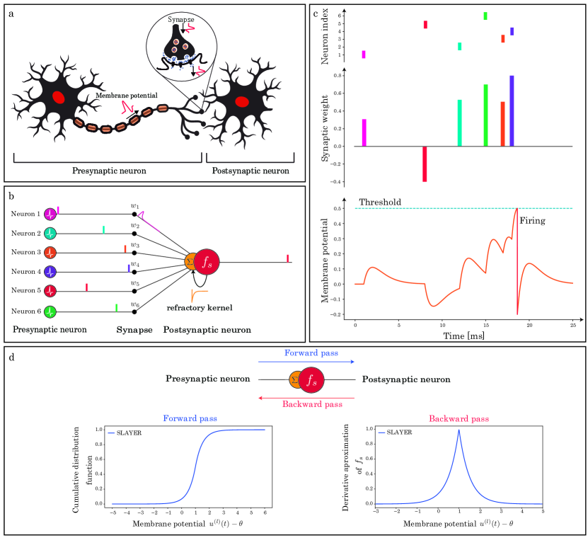
Figure 1: Illustration of fundamental components of SNN. (a) Biological information and signal processing between presynaptic and postsynaptic neurons in SNN. (b) A spiking neuron processes and communicates binary spiking events over time. (c) The postsynaptic neuron changes the membrane potential through each layer of the post-synaptic potential (PSP). It generates the output spikes when the membrane potential reaches the neuronal firing threshold [14]. (d) The cumulative distribution function (“Forward pass”) of our surrogate gradient and itself (“Backward pass”) [6].

2 Related Works

2.1 Spiking Neuron

SNN consists of spiking neurons that model the behavior of biological neurons and handle the firing timing of the spikes. Owing to the differences in approximations, several spiking neuron models have been proposed, such as the integrate-fire (IF) [16], leaky-integrate-and-fire (LIF) [17], Izhikevich [18], and Hodgkin-Huxley model [19]. In this study, we adopt the spike response model (SRM) [20] to deal with the refractory period (Section 3).

The refractory period is an essential function of biological neurons to suppress the spike firing. Spike firing occurs when the neuron’s membrane potential exceeds the firing threshold. From a biological perspective, the membrane potential is calculated using PSP, representing the electrical signals converted from the chemical signals. These behaviors are represented within the chemical synapse model shown in Figure 1 (a) [21]. SRM was implemented to approximate this synaptic model better than IF/LIF neurons, which are widely used in SNNs.

2.2 Training of Spiking Neural Networks

It is well-known that SNNs are difficult to train due to non-differential spike trains. Researchers are working on this problem, and their solutions can be divided into two approaches: first, the ANN-SNN conversion [22, 24, 25, 23], and second, the usage of the surrogate gradient [7, 8, 6, 5, 9]. The ANN-SNN conversion method uses the trained ANN parameters of SNN. The sophisticated and state-of-the-art ANN model can be reused through this method. However, this conversion approach requires many time-steps during inference and increase the power consumption. In contrast, the surrogate gradient is used to directly train SNNs by approximating the gradient. The surrogate gradient approach was adopted since the model obtained by surrogate gradient requires far fewer inference time-steps than the ANN-SNN conversion model [26].

2.3 Normalization

One of the techniques that have contributed to the success of ANNs is Batch Normalization (BN) [27]. BN is used to reduce the internal covariate shift, leading to a smooth landscape [28] while corresponding to the homeostatic plasticity mechanism of BNNs [29]. Using a mini-batch, BN computes the sample mean and standard deviation (STD). Meanwhile, several variants have been proposed to compute the sample mean and STD, such as Layer Normalization (LN) [30], Instance Normalization (IN) [31], and Group Normalization (GN) [32]. In particular, LN is effective at stabilizing the hidden state dynamics in recurrent neural networks for time-series processing [30].

Several normalization methods have also been proposed in the field of SNNs, such as threshold-dependent BN (tdBN) [33] and BN through time (BNTT) [34]. Thus, tdBN incorporates the firing threshold into BN, whereas BNTT computes BN at each time step. Furthermore, some studies used BN as is [35]. These studies applied the normalization to the membrane potential. In contrast, our method was applied to PSP, as shown in Figure 2 (b), to simplify the normalization form (Section 4).

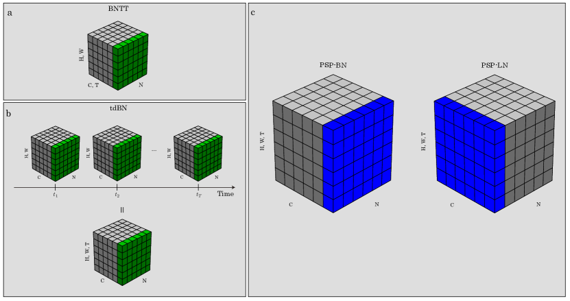
Figure 2: Normalization methods for spiking neural networks (SNNs). Each subplot shows a feature map (a, b) or post-synaptic input (b) tensor, with N as the batch axis, C as the channel axis, (H, W) as the spatial axis, and T as the time axis in the figure. Green voxels (a, b), previous methods, and blue (b), our proposed method, are normalized by the same second central moment and uncentered second moment, respectively.

3 Spiking Neural Networks based on Spike Response Model

In this section, we describe the SNN used in this study. Our SNN is constructed using SRM [20]; it uses SLAYER [6] as the surrogate gradient function to train the SRM.

3.1 Spike Response Model

We adopt SRM as a spiking neuron model [20]. SRM model is based on combining the effects of the incoming spike arriving at the spiking neuron. It also has a function to the spike firing when the membrane potential $u(t)(t=1,2,\cdots,T)$ reaches the firing threshold. Figures 1 (b) and (c) indicate the behavior of this model. The equations are given as follows:

$$u_{i}(t) = \sum_{j}w_{ij}(\varepsilon\ast s_{j})(t)+(\nu\ast s_{i})(t),$$ (1)

$$s_{i}(t) = f_{s}(u_{i}(t)-\theta),$$ (2)

where $w_{i,j}$ is the synaptic weight from the presynaptic neuron $j$ to the postsynaptic neuron $i$. $s_{j}(t)$ is the spike train inputted from the presynaptic neuron $j$, $s_{i}(t)$ is the output spike train of the postsynaptic neuron $i$, $\ast$ is a temporal convolution operator, and $\theta$ is a threshold used to control the spike generation. $f_{s}$ is the Heaviside step function, which fires the spike when the membrane potential $u_{i}(t)$ exceeds the firing threshold $\theta$. In addition, $\varepsilon(\cdot)$ and $\nu(\cdot)$ are the spike response and refractory kernels formulated using the exponential function as follows:

$$\varepsilon(t) = \frac{t}{\tau_{s}}e^{1-\frac{t}{\tau_{s}}},$$ (3)

$$\nu(t) = -2\theta e^{-\frac{t}{\tau_{r}}},$$ (4)

where $\tau_{s}$ and $\tau_{r}$ are the time constants of spike response and refractory kernels, respectively. Note that $\varepsilon\ast s_{j}(t)$ represents the PSP.

3.2 Multiple Layers Spike Response Model

By using Equations (1) and (2), the SNNs with multi-layers can be described as follows:

$$\displaystyle\bm{a}^{(l)}(t) = (\varepsilon\ast\bm{s}^{(l)})(t),$$ (5)

$$\displaystyle\bm{u}^{(l+1)}(t) = \bm{W}^{(l)}\bm{a}^{(l)}(t)+(\nu\ast\bm{s}^{(l+1)})(t),$$ (6)

$$\displaystyle\bm{s}^{(l+1)}(t) = f_{s}(\bm{u}^{(l+1)}(t)),$$ (7)

where $\bm{a}^{(l)}(t)\in\mathbb{R}_{\geq 0}^{\mathrm{C}\times\mathrm{W}\times\mathrm{H}}$ and $\bm{s}^{(l)}(t)\in\{0,1\}^{\mathrm{C}\times\mathrm{W}\times\mathrm{H}}$ are the PSP and input spike tensor of time step $t$; $\mathrm{C}$ is the number of channels; and $\mathrm{W}$ and $\mathrm{H}$ are the width and height of the input spike tensor, respectively. Since $\bm{a}^{(l)}(t)$ does not take a value less than zero, we consider an excitatory neuron. Furthermore, $\bm{W}^{(l)}\in\mathbb{R}^{M}$ is the weight matrix representing the synaptic strengths between the spiking neurons in $l$ and $l+1$ layers; $M$ is the number of neurons of $l+1$-th layer.

3.3 Deep SNNs by Pre-activation Blocks

Deep neural network are essential to recognize complex input patterns. In particular, ResNet is widely used in ANNs [15, 36], and its use in SNNs is expanding.

The ResNet’s networks are divided into the pre-activation and post-activation residual blocks as follows (Figure 3):

$$\displaystyle{\sf Pre}:\bm{h}^{(k+1)}(t) = \bm{h}^{(k)}(t)+G(\bm{h}^{(k)}(t)),$$ (8)

$$\displaystyle{\sf Post}:\bm{h}^{(k+1)}(t) = F(\bm{h}^{(k)}(t)+G(\bm{h}^{(k)}(t))),$$ (9)

where $\bm{h}^{(k)}$ and $\bm{h}^{(k+1)}$ are the input and output in the $k+1$ block, respectively. $G$ represents the residual function, corresponding to “Conv-Func-Conv” and “Func-Conv-Func-Conv” in Figure 3; $F$ represents the Func layer (“Spike-PSP-Norm”). Note that the refractory period is used in $F$. In the experimental section, we compare these blocks and show that deep SNNs can be trained using the pre-activated residual blocks. This result shows that identity mapping is an essential tool to train the deep SNNs, similar to ANNs [36].

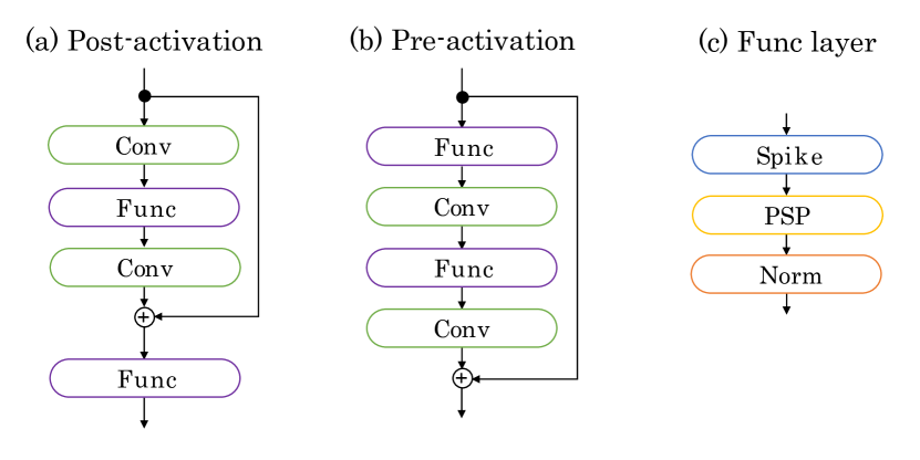
Figure 3: Network blocks. (a) Post-activation residual block, (b) Pre-activation residual block, and (c) Func layer. Postsynaptic potential (PSP) and Norm in the Func layer represent Equation (5) and normalization. Spike represents $f_{s}(.+r)$, where $r$ is the refractory period.

3.4 Surrogate-Gradient

We use SLAYER [6] as one of the surrogate gradient algorithms to tarin the SNN with multi-layers. In SLAYER, the derivative of the spike activation function $f_{s}$ of the $l+1$ layer is approximated as follows (Figure 1 (d)):

$$\displaystyle\bm{\rho}^{(l+1)}(t) = \frac{1}{\alpha}(-\beta|\bm{u}^{(l+1)}(t)-\bm{\theta}|),$$ (10)

where $\alpha$ and $\beta$ are hyperparameters, and $\bm{\theta}\in\mathbb{R}^{M}$ is the firing threshold. SLAYER can be used to train SRM as described in [6].

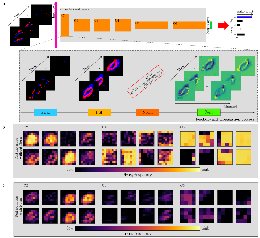
Figure 4: (a) Overview of the forward propagation phase using postsynaptic potential (PSP) normalization on the N-MNIST dataset. (b) Example of feature maps, which are integrated along the time axis, without PSP normalization. (c) As in (b) but for feature maps with it. PSP normalization controls the activity of the network and prevents the over-firing of the neurons.

4 Normalization of Postsynaptic Potential

In this section, we explain the derivation of our normalization, which is called postsynaptic-potential normalization, as shown in Figure 4 (a).

As the depth of the SNN becomes deeper, it becomes more difficult to control spike firing properly (Figures 4 (b) and (c)). To tackle this problem, we first introduce the following typical normalization into the PSP.

$$\displaystyle\bm{\hat{u}}^{(l+1)}(t) = \bm{W}^{(l)}\bm{\hat{a}}^{(l)}(t)+(\nu\ast\bm{s}^{(l+1)})(t),$$ (11)

$$\displaystyle\bm{\hat{a}}^{(l)}(t) = \frac{\bm{a}^{(l)}(t)-\mathbb{E}_{X}[\bm{a}^{(l)}]}{\sqrt{\mathbb{V}_{X}[\bm{a}^{(l)}]+\lambda}}\odot\gamma+\xi,$$ (12)

where $\gamma$ and $\xi$ are trainable parameters; each variable of $\mathbb{E}_{X}[\bm{a}^{(l)}]$ and $\mathbb{V}_{X}[\bm{a}^{(l)}]$ is approximate as follows:

$$\displaystyle\mathbb{E}_{X}[a^{(l)}_{i}] \approx \frac{1}{X}\sum_{x=1}^{X}a^{(l)}_{i}(x),$$ (13)

$$\displaystyle\mathbb{V}_{X}[a^{(l)}_{i}] \approx \frac{1}{X}\sum_{x=1}^{X}(a^{(l)}_{i}(x)-\mathbb{E}_{X}[a^{(l)}_{i}])\odot(a^{(l)}_{i}(x,t)-\mathbb{E}_{X}[a^{(l)}_{i}]),$$ (14)

where $a^{(l)}_{i}(x)$ represents the $x$-th variable required to compute these statistics of the $i$-th variable of $\bm{a}^{(l)}\in\mathbb{R}_{\geq 0}^{\mathrm{C}\times\mathrm{W}\times\mathrm{H}\times\mathrm{N}\times\mathrm{T}}$ ($N$ is the mini-batch size), and $X$ depends on what kind of summation to compute. For example, if we compute these equations as in BN, $X=W\times H\times N\times T$. In addition, if we compute them as in LN, $X=W\times H\times C\times T$. Note that the normalization to PSP means that it inserts before the convolution or fully connected layers. This position differs from the other normalization ones, which use normalization to the membrane potential [35, 34, 33].

As shown in Equation (12), $\bm{\hat{a}}^{(l)}(t)$ may take minus. Therefore, $\bm{\hat{a}}^{(l)}(t)<0$ is not valid since neurons of SLAYER represent excitatory neurons. This phenomenon clearly arises from the trainable parameter $\xi$ and the shift parameter $\mathbb{E}_{X}[\bm{a}^{(l)}]$. Thus, we modify Equation (12) as follows:

$$\displaystyle\bm{\hat{a}}^{(l)}(t) = \frac{\bm{a}^{(l)}(t)}{\sqrt{\mathbb{V}_{X}[\bm{a}^{(l)}]+\lambda}}\odot\gamma.$$ (15)

Next, we consider the case when $\bm{\hat{u}}^{(l+1)}(t)$ reaches the firing threshold $\bm{\theta}$.

$$\displaystyle\bm{\theta} = \bm{W}^{(l)}\bm{\hat{a}(t)}+(\nu\ast\bm{s}^{(l+1)})(t),$$ (16)

$$= \bm{\hat{W}}^{(l)}\frac{\bm{a}^{(l)}(t)}{\sqrt{\mathbb{V}_{X}[\bm{a}^{(l)}]+\lambda}}+(\nu\ast\bm{s}^{(l+1)})(t).$$ (17)

Here, we merged the trainable parameter $\gamma$ and the weight matrix $\bm{W}^{(l)}$ into $\bm{\hat{W}}^{(l)}$. This merging is possible because of the normalization performed before multiplying $\bm{W}^{(l)}$. Then, we express Equation (17) as follows:

$$\displaystyle\bm{\hat{W}}^{(l)}\bm{a}^{(l)}(t) = \sqrt{\mathbb{V}_{X}[\bm{a}^{(l)}]+\lambda}(\bm{\theta}-\nu\ast\bm{s}^{(l+1)}(t))\ \ \ \coloneqq\ \ \ \hat{\bm{\theta}}.$$ (18)

Equation (18) shows that the firing threshold varies dynamically, which is consistent with the activity of cortical neurons in the human brain [38, 39, 40, 37]. The refractory period $(\nu\ast\bm{s}^{(l+1)})(t)$ and $\sqrt{\mathbb{V}_{X}[\bm{a}^{(l)}]+\lambda}$ can decrease $\hat{\bm{\theta}}$ and scaling, respectively.

Next, we focus on the scale factor $\sqrt{\mathbb{V}_{X}[\bm{a}^{(l)}]+\lambda}$. As shown in Equation (18), the firing threshold $\hat{\bm{\theta}}$ becomes larger as the variance (second central moment) $\mathbb{V}_{X}[\bm{a}^{(l)}]$ increases. However, considering the behavior of the membrane potential, $\hat{\bm{\theta}}$ should become larger when the value of PSP (not variance) increases. Thus, we modify the equation as follows.

$$\displaystyle\bm{\hat{a}}^{(l)}(t) = \frac{\bm{a}^{(l)}(t)}{\sqrt{\mathbb{E}_{X}[(\bm{a}^{(l)})^{2}]+\lambda}},$$ (19)

where $\mathbb{E}_{X}[(\bm{a}^{(l)})^{2}]$ represents the second raw moment consisting of the following variable,

$$\displaystyle\mathbb{E}_{X}[(a^{(l)}_{i})^{2}] \approx \frac{1}{X}\sum_{x=1}^{X}a^{(l)}_{i}(x)\odot a^{(l)}_{i}(x).$$ (20)

By using this equation, we do not have to compute the mean beforehand, in contrast to using the variance.

In addition to $\mathbb{E}_{X}[(\bm{a}^{(l)})^{2}]$, there is a hyperparameter $\lambda$ in the scale factor. $\lambda$ is usually set to a small constant, e.g., $\lambda=10^{-3}$ because it plays the role of the numerical stability. Figure 5 shows the relationship between $\mathbb{E}_{X}[(a^{(l)}_{i})^{2}]$ and $\hat{\theta}$ when changing $\theta$ and $\lambda$. As shown in this figure, $\hat{\theta}$ monotonically decreases as $\mathbb{E}_{X}[(a^{(l)}_{i})^{2}]$ decreases. In particular, $\hat{\theta}$ is close to zero when $\lambda$ is sufficiently small, regardless of the initial threshold $\theta$. $\hat{\theta}\approx 0$ means that spikes fire at all times even if the membrane potential is significantly small, making it difficult to train a proper model. Thus, we set a relatively large value ($\lambda=0.1$) as the default value.

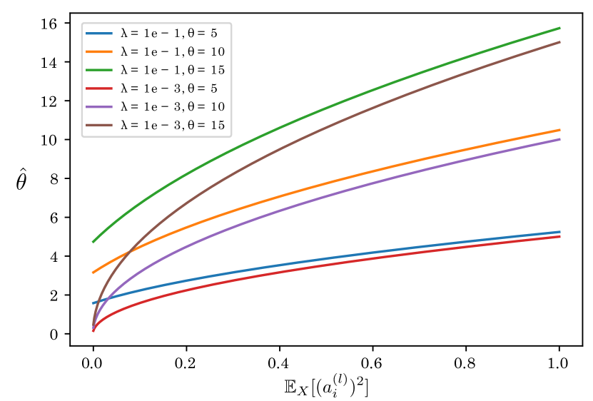
Figure 5: Relationship between $\mathbb{E}_{X}[(a^{(l)}_{i})^{2}]$ and $\hat{\theta}$.

5 Experiments

In this section, we evaluate two PSP normalizations: BN (the most common normalization) and LN (which is effective in time-series processing, such as SNN). We called them PSP-BN ($X=W\times H\times N\times T$) and PSP-LN ($X=W\times H\times C\times T$).

5.1 Experimental Setup

We evaluated PSP-BN and PSP-LN on the spatio-temporal event and static image datasets. We used N-MNIST [12] and F-MNIST [13]. N/F-MNISTs are widely used datasets containing 60K training and 10K test samples with 10 classes. Each size is $34\times 34\times 30000$ events (N-MNIST), and $28\times 28$ pixels (F-MNIST). We partitioned the 60K data using 54K and 6K as our training and validation data, respectively. We also resized the F-MNIST image from $28\times 28$ to $34\times 34$ to achieve higher accuracy.

We evaluated the performance of several spiking convolutional neural network models, such as six-convolutional layers on both datasets and 14-convolutional layers on N/F-MNIST. We also used more deep models, such as ResNet-106 on N-MNIST and F-MNIST, respectively.

We used hyperparameters shown in Table 1 in all experiments and implemented by PyTorch. We used the default initialization of PyTorch and showed the best accuracies of all models. All experiments were conducted using a single Tesla V100 GPU. In addition to this computational resource limitation, we randomly sampled 6K of the training data for both datasets to train in each epoch since SLAYER requires a significant amount of time to train.

Hyperparameter	N-MNIST	F-MNIST
$\tau_{s}$	10	10
$\tau_{r}$	10	10
$\alpha$	10	10
$\beta$	10	10
$\theta$	10	10
optimizer	AdaBelief	AdaBelief
learning rate	$10^{-2}$	$10^{-2}$
weight decay	$10^{-4}$	$10^{-4}$
weight scale	10	10
mini-batch size	10	10
time step	300	100
epoch	100	100

Table 1: Hyperparameter setting on N-MNIST and F-MNIST.

5.2 Effectiveness of Postsynaptic Potential Normalization

We first evaluate the effectiveness of our normalizations. Table 2 presents the accuracies of PSP-BN and PSP-LN and other approaches. Note that we set our normalization before the convolution as described in Section 4, which is different from the position proposed in previous studies [35, 34, 33]. This table illustrates that PSP-BN and PSP-LN achieve high accuracies on both datasets compared to the other approaches.

We also investigate the effect of the proposed method on the firing rate. Figures 6 and 7 show the firing rates of each method. As shown in Figure 6, our normalized models can suppress the firing rate in most layers compared to the unnormalized model. Furthermore, from Figure 7 and Table 2 show that our normalized models can simultaneously achieve high classification accuracy and low firing rate compared to other normalizations. These results verifies the effectiveness of our normalizations.

Method	Dataset	Network architecture	Acc. (%)
BN [35]	N-MNIST	34$\times$34$\times$2-8c3n-{16c3n}*5-16c3n-{32c3n}*5-10	85.1
BNTT [34]	N-MNIST	34$\times$34$\times$2-8c3n-{16c3n}*5-16c3n-{32c3n}*5-10	90.0
tdBN [33]	N-MNIST	34$\times$34$\times$2-8c3n-{16c3n}*5-16c3n-{32c3n}*5-10	81.8
PSP-BN	N-MNIST	34$\times$34$\times$2-n8c3-{n16c3}*5-n16c3-{n32c3}*5-10	97.4
PSP-LN	N-MNIST	34$\times$34$\times$2-n8c3-{n16c3}*5-n16c3-{n32c3}*5-10	98.2
None	N-MNIST	34$\times$34$\times$2-8c3-{16c3}*5-16c3-{32c3}*5-10	40.6
BN [35]	F-MNIST	34$\times$34-16c3n-{32c3n}*5-32c3n-{64c3n}*5-10	10
BNTT [34]	F-MNIST	34$\times$34-16c3n-{32c3n}*5-32c3n-{64c3n}*5-10	10
tdBN [33]	F-MNIST	34$\times$34-16c3n-{32c3n}*5-32c3n-{64c3n}*5-10	40.5
PSP-BN	F-MNIST	34$\times$34-n16c3-{n32c3}*5-n32c3-{n64c3}*5-10	88.6
PSP-LN	F-MNIST	34$\times$34-n16c3-{n32c3}*5-n32c3-{n64c3}*5-10	89.1
None	F-MNIST	34$\times$34-16c3-{32c3}*5-32c3-{64c3}*5-10	84.1

Table 2: Accuracies of N-MNIST and F-MNIST obtained from different methods. PSP-BN and PSP-LN are our normalization methods, and None is the model without normalization. Here, “C”, “n”, and “d” represent the convolution, normalization, and dense layers, respectively. In addition, each layer and spatial dimension in the network are separated by “-” and “x”.

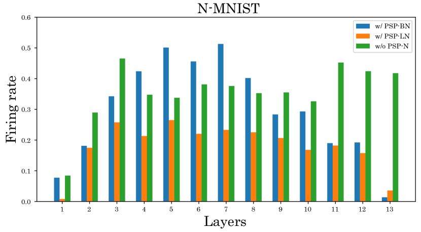
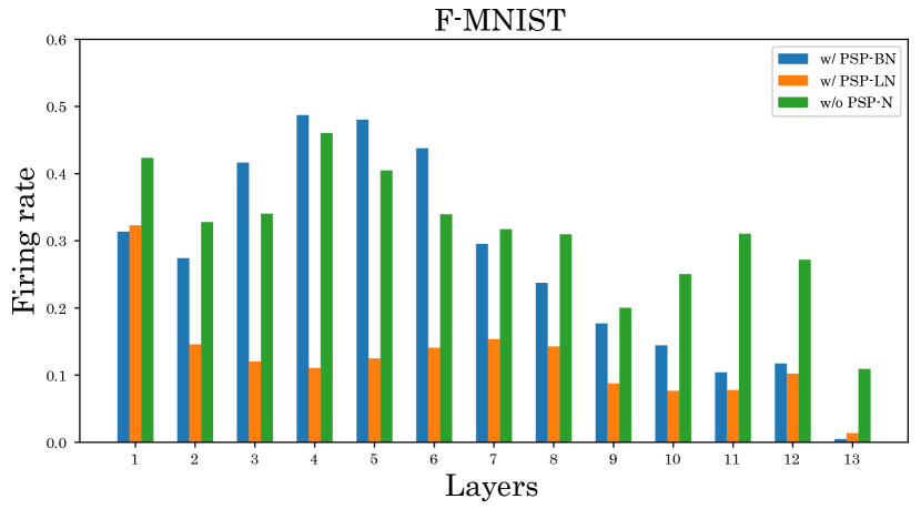
Figure 6: Comparison of firing rates. The top is N-MNIST and the bottom is F-MNIST.

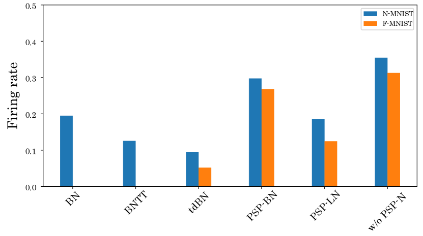
Figure 7: Total firing rates of each model.

5.3 Accuracy Dependency on Varying Hyperparameters

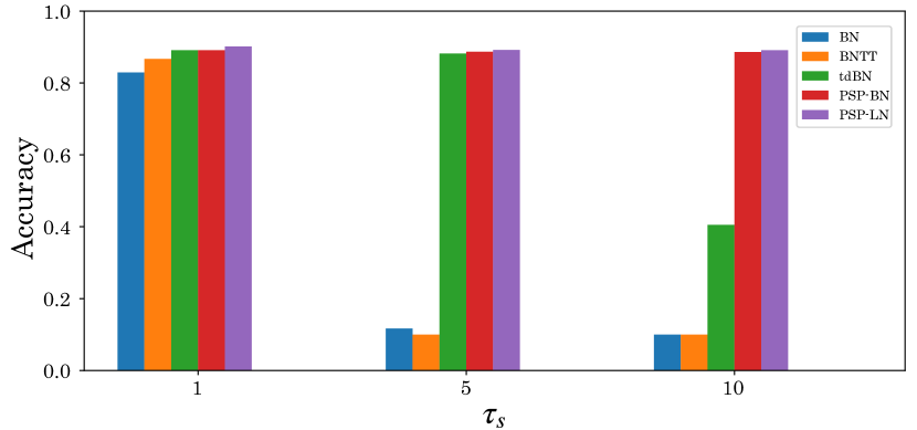
Figure 8: Accuracy comparison of F-MNIST dataset with respect to changing hyperparameter $\tau_{s}$.

Some authors pointed out that the tuning of hyperparameter $\tau_{s}$ is essential to achieve higher accuracy [41]. Therefore, to investigate the effect of $\tau_{s}$, we compare the accuracy with respect to changing $\tau_{s}$. Figure 8 shows F-MNIST’s accuracies of each method for $\tau_{s}=\{1,5,10\}$. As shown in this figure, the models with PSP-BN/LN maintain the accuracy whereas others deteriorate the accuracies. This result shows that the model becomes robust to $\tau_{s}$ using our normalizations.

In addition to $\tau_{s}$, we show the influence of $\lambda$. Figure 9 shows the performance when changing $\lambda$. As shown in this figure, the classification performance of PSP-BN becomes worse for a sufficient small value of $\lambda$. This result verifies the plausibility of our discussion in Section 4.

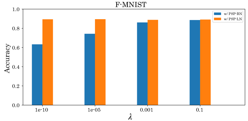
Figure 9: Accuracy comparison of F-MNIST with respect to changing $\lambda$.

5.4 Performance Evaluation of Deep SNNs by Residual Modules

Meshod	Dataset	Network architecture	Acc. (%)
PSP-BN	N-MNIST	Post-activation ResNet-106	10.0
PSP-BN	N-MNIST	Pre-activation ResNet-106	75.4
PSP-LN	N-MNIST	Post-activation ResNet-106	10.0
PSP-LN	N-MNIST	Pre-activation ResNet-106	86.8
PSP-BN	F-MNIST	Post-activation ResNet-106	10.0
PSP-BN	F-MNIST	Pre-activation ResNet-106	81.6
PSP-LN	F-MNIST	Post-activation ResNet-106	10.0
PSP-LN	F-MNIST	Pre-activation ResNet-106	82.1

Table 3: Performance comparison using post-activation and pre-activation residual blocks. We use ResNet-106 on N-MNIST and F-MNIST datasets, respectively.

Finally, we evaluate the performance of SNNs using the residual blocks. Table 3 shows the performance of SNNs using the pre-activation and post-activation residual blocks. As shown in this table, the accuracy is substantially improved using the pre-activation residual blocks. This result shows that the post-activation employed in previous studies without refractory period [33, 5, 11] is unsuitable for SNNs with a refractory period. Thus, while ensuring the biological plausibility, due to the refractory period, we can obtain deep SNNs beyond 100 layers using our normalizations and pre-activation residual blocks.

6 Conclusion

In this study, we proposed an appropriate normalization method for SNN. The proposed normalization removes the subtraction term from the standard normalization and uses the second raw moment as the denominator. Our normalized models outperformed other normalized models by inserting this simple normalization before the convolutional layer. Moewover, our proposed model with pre-activation residual blocks can train with more than 100 layers without any other special techniques dedicated to SNNs. In future studies, we will analyze more details and verify the effect on other datasets. Furthermore, we aim to extend postsynaptic normalization based on BN to develop robust normalization techniques for the thresholds in spiking neurons.

References

- [1] Maass, Wolfgang. "Networks of spiking neurons: the third generation of neural network models." Neural networks 10, no. 9 (1997): 1659-1671.
- [2] Akopyan, Filipp, Jun Sawada, Andrew Cassidy, Rodrigo Alvarez-Icaza, John Arthur, Paul Merolla, Nabil Imam et al. "Truenorth: Design and tool flow of a 65 mw 1 million neuron programmable neurosynaptic chip." IEEE transactions on computer-aided design of integrated circuits and systems 34, no. 10 (2015): 1537-1557.
- [3] Davies, Mike, Narayan Srinivasa, Tsung-Han Lin, Gautham Chinya, Yongqiang Cao, Sri Harsha Choday, Georgios Dimou et al. "Loihi: A neuromorphic manycore processor with on-chip learning." Ieee Micro 38, no. 1 (2018): 82-99.
- [4] Maguire, Liam P., T. Martin McGinnity, Brendan Glackin, Arfan Ghani, Ammar Belatreche, and Jim Harkin. "Challenges for large-scale implementations of spiking neural networks on FPGAs." Neurocomputing 71, no. 1-3 (2007): 13-29.
- [5] Lee, Chankyu, Syed Shakib Sarwar, Priyadarshini Panda, Gopalakrishnan Srinivasan, and Kaushik Roy. "Enabling spike-based backpropagation for training deep neural network architectures." Frontiers in neuroscience 14 (2020): 119.
- [6] Shrestha, Sumit B., and Garrick Orchard. "Slayer: Spike layer error reassignment in time." Advances in Neural Information Processing System 31 (2018).
- [7] Wu, Yujie, Lei Deng, Guoqi Li, Jun Zhu, and Luping Shi. "Spatio-temporal backpropagation for training high-performance spiking neural networks." Frontiers in neuroscience 12 (2018): 331.
- [8] Zenke, Friedemann, and Surya Ganguli. "Superspike: Supervised learning in multilayer spiking neural networks." Neural computation 30, no. 6 (2018): 1514-1541.
- [9] Zhang, Wenrui, and Peng Li. "Temporal spike sequence learning via backpropagation for deep spiking neural networks." Advances in Neural Information Processing System 33 (2020):12022-12033.
- [10] Rumelhart, David E., Geoffrey E. Hinton, and Ronald J. Williams. "Learning representations by back-propagating errors." nature 323, no. 6088 (1986): 533-536.
- [11] Fang, Wei, Zhaofei Yu, Yanqi Chen, Tiejun Huang, Timothée Masquelier, and Yonghong Tian. "Deep Residual Learning in Spiking Neural Networks." Advances in Neural Information Processing System 34.
- [12] Orchard, Garrick, Ajinkya Jayawant, Gregory K. Cohen, and Nitish Thakor. "Converting static image datasets to spiking neuromorphic datasets using saccades." Frontiers in neuroscience 9 (2015): 437.
- [13] Xiao, Han, Kashif Rasul, and Roland Vollgraf. "Fashion-mnist: a novel image dataset for benchmarking machine learning algorithms." arXiv preprint arXiv:1708.07747 (2017).
- [14] Comsa, Iulia M., Krzysztof Potempa, Luca Versari, Thomas Fischbacher, Andrea Gesmundo, and Jyrki Alakuijala. "Temporal coding in spiking neural networks with alpha synaptic function." In ICASSP 2020-2020 IEEE International Conference on Acoustics, Speech and Signal Processing (ICASSP), pp. 8529-8533. IEEE, 2020.
- [15] He, Kaiming, Xiangyu Zhang, Shaoqing Ren, and Jian Sun. "Deep residual learning for image recognition." In Proceedings of the IEEE conference on computer vision and pattern recognition, pp. 770-778. 2016.
- [16] Lapique, Louis. "Recherches quantitatives sur l’excitation electrique des nerfs traitee comme une polarization." Journal of Physiology and Pathololgy 9 (1907): 620-635.
- [17] Stein, Richard B. "A theoretical analysis of neuronal variability." Biophysical Journal 5, no. 2 (1965): 173-194.
- [18] Izhikevich, Eugene M. "Simple model of spiking neurons." IEEE Transactions on neural networks 14, no. 6 (2003): 1569-1572.
- [19] Hodgkin, Alan L., and Andrew F. Huxley. "A quantitative description of membrane current and its application to conduction and excitation in nerve." The Journal of physiology 117, no. 4 (1952): 500-544.
- [20] Gerstner, Wulfram, and Werner M. Kistler. Spiking neuron models: Single neurons, populations, plasticity. Cambridge university press, 2002.
- [21] Rall, Wilfrid. "Distinguishing theoretical synaptic potentials computed for different soma-dendritic distributions of synaptic input." Journal of neurophysiology 30, no. 5 (1967): 1138-1168.
- [22] Diehl, Peter U., Daniel Neil, Jonathan Binas, Matthew Cook, Shih-Chii Liu, and Michael Pfeiffer. "Fast-classifying, high-accuracy spiking deep networks through weight and threshold balancing." In 2015 International joint conference on neural networks (IJCNN), pp. 1-8. ieee, 2015.
- [23] Li, Yuhang, Shikuang Deng, Xin Dong, Ruihao Gong, and Shi Gu. "A Free Lunch From ANN: Towards Efficient, Accurate Spiking Neural Networks Calibration." In International Conference on Machine Learning, pp.6316-6325. PMLR, 2021.
- [24] Rueckauer, Bodo, Iulia-Alexandra Lungu, Yuhuang Hu, Michael Pfeiffer, and Shih-Chii Liu. "Conversion of continuous-valued deep networks to efficient event-driven networks for image classification." Frontiers in neuroscience 11 (2017): 682.
- [25] Sengupta, Abhronil, Yuting Ye, Robert Wang, Chiao Liu, and Kaushik Roy. "Going deeper in spiking neural networks: VGG and residual architectures." Frontiers in neuroscience 13 (2019): 95.
- [26] Diehl, Peter U., and Matthew Cook. "Unsupervised learning of digit recognition using spike-timing-dependent plasticity." Frontiers in computational neuroscience 9 (2015): 99.
- [27] Ioffe, Sergey, and Christian Szegedy. "Batch normalization: Accelerating deep network training by reducing internal covariate shift." In International conference on machine learning, pp. 448-456. PMLR, 2015.
- [28] Santurkar, Shibani, Dimitris Tsipras, Andrew Ilyas, and Aleksander Mądry. "How does batch normalization help optimization?." In Proceedings of the 32nd international conference on neural information processing systems, pp. 2488-2498. 2018.
- [29] Shen, Yang, Julia Wang, and Saket Navlakha. "A correspondence between normalization strategies in artificial and biological neural networks." Neural Computation 33, no. 12 (2021): 3179-3203.
- [30] Ba, Jimmy Lei, Jamie Ryan Kiros, and Geoffrey E. Hinton. "Layer normalization." arXiv preprint arXiv:1607.06450 (2016).
- [31] Ulyanov, Dmitry, Andrea Vedaldi, and Victor Lempitsky. "Instance normalization: The missing ingredient for fast stylization." arXiv preprint arXiv:1607.08022 (2016).
- [32] Wu, Yuxin, and Kaiming He. "Group normalization." In Proceedings of the European conference on computer vision (ECCV), pp. 3-19. 2018.
- [33] Zheng, Hanle, Yujie Wu, Lei Deng, Yifan Hu, and Guoqi Li. "Going Deeper With Directly-Trained Larger Spiking Neural Networks." In Proceedings of the AAAI Conference on Artificial Intelligence, vol. 35, no. 12, pp. 11062-11070. 2021.
- [34] Kim, Youngeun, and Priyadarshini Panda. "Revisiting batch normalization for training low-latency deep spiking neural networks from scratch." Frontiers in neuroscience 15 (2021): 773954.
- [35] Ledinauskas, Eimantas, Julius Ruseckas, Alfonsas Juršėnas, and Giedrius Buračas. "Training deep spiking neural networks." arXiv preprint arXiv:2006.04436 (2020).
- [36] He, Kaiming, Xiangyu Zhang, Shaoqing Ren, and Jian Sun. "Identity mappings in deep residual networks." In European conference on computer vision, pp. 630-645. Springer, Cham, 2016.
- [37] Aertsen, Adrianus, and Valentino Braitenberg, eds. Brain theory: biological basis and computational principles. Elsevier, 1996.
- [38] Frankenhaeuser, B., and Å. B. Vallbo. "Accommodation in myelinated nerve fibres of Xenopus laevis as computed on the basis of voltage clamp data." Acta Physiologica Scandinavica 63, no. 1-2 (1965): 1-20.
- [39] Schlue, W. R., D. W. Richter, K. H. Mauritz, and A. C. Nacimiento. "Responses of cat spinal motoneuron somata and axons to linearly rising currents." Journal of Neurophysiology 37, no. 2 (1974): 303-309.
- [40] Stafstrom, CARL E., PETER C. Schwindt, J. A. Flatman, and WAYNE E. Crill. "Properties of subthreshold response and action potential recorded in layer V neurons from cat sensorimotor cortex in vitro." Journal of neurophysiology 52, no. 2 (1984): 244-263.
- [41] Fang, Wei, Zhaofei Yu, Yanqi Chen, Timothée Masquelier, Tiejun Huang, and Yonghong Tian. "Incorporating learnable membrane time constant to enhance learning of spiking neural networks." In Proceedings of the IEEE/CVF International Conference on Computer Vision, pp. 2661-2671. 2021.