Introduction to the combinatorial atlas

Abstract.

We give elementary self-contained proofs of the strong Mason conjecture recently proved by Anari et. al [ALOV18] and Brändén–Huh [BH20], and of the classical Alexandrov–Fenchel inequality. Both proofs use the combinatorial atlas technology recently introduced by the authors [CP21]. We also give a formal relationship between combinatorial atlases and Lorentzian polynomials.

1. Introduction

In this paper we tell three interrelated but largely independent stories. While we realize that this sounds self-contradictory, we insist on this description. We prove no new results, nor do we claim to give new proofs of known results. Instead, we give a new presentation of the existing proofs.

Our goal is explain the combinatorial atlas technology from [CP21] in three different contexts. The idea is to both give a more accessible introduction to our approach and connect it to other approaches in the area. Although one can use this paper as a companion to [CP21], it is written completely independently and aimed at a general audience.

$(1)$  Strong Mason conjecture claims ultra-log-concavity of the number of independent sets of matroid according to its size. This is perhaps the most celebrated problem recently resolved in a series of paper culminating with independent proofs by Anari et. al [ALOV18] and Brändén–Huh [BH20]. These proofs use the technology of Lorentzian polynomials, which in turn substantially simplify earlier heavily algebraic tools.

In our paper [CP21], we introduce the combinatorial atlas technology motivated by geometric considerations of the Alexandrov–Fenchel inequality. This allowed us, among other things, to prove an advanced generalization of the strong Mason conjecture to a large class of greedoids. The conjecture itself and its refinements followed easily from our more general results. Our first story is a self-contained streamlined proof of just this conjecture, without the delicate technical details necessary for our generalizations.

$(2)$  Lorentzian polynomials as a technology is an interesting concept in its own right. In [BH20], the authors showed not only how to prove matroid inequalities, but also how to place the technology in the context of ideas and approaches in other areas, including the above mentioned Alexandrov–Fenchel inequality.

We do something similar in our second story, by showing that the theory of Lorentzian polynomials is a special case of the theory of combinatorial atlases. More precisely, for every Lorentzian polynomial we construct a combinatorial atlas which mimics the polynomial properties and allows to derive the same conclusions.

$(3)$  The Alexandrov–Fenchel inequality  is the classical geometric inequality which remains deeply mysterious. There are several algebraic and analytic proofs, all of them involved and technical, to different degree. Much of the combinatorial atlas technology owes to our deconstruction of the insightful recent proof in [SvH19] by Shenfeld and van Handel.

In the third story, we proceed in the reverse direction, and prove the Alexandrov–Fenchel inequality by the tools of the combinatorial atlas. The resulting proof is similar to that in [SvH19], but written in a different language and filling the details not included in [SvH19]. Arguably, this is the first exposition of the proof of the Alexandrov–Fenchel inequality that is both elementary and self-contained.

The paper structure is very straightforward. After the short notation section (Section 2), we define the combinatorial atlas and state its properties (Section 3). This is a prequel to all three sections that follow, all of which are independent from each other, and cover items $(1)$, $(2)$ and $(3)$. At risk of repeating ourselves, let us emphasize that these three Sections 4, 5 and 6 can be read in any order. We conclude with brief final remarks in Section 7. For further background and historical remarks, see the extensive $\S$16 and $\S$17 in [CP21].

2. Definitions and notations

We use  $[n]=\{1,\ldots,n\}$,  $\mathbb{N}=\{0,1,2,\ldots\}$,  $\operatorname{\mathbb{Z}}_{+}=\{1,2,\ldots\}$,  $\mathbb{R}_{\geq 0}=\{x\geq 0\}$  and  $\mathbb{R}_{>0}=\{x>0\}$. For a subset  $S\subseteq X$  and element  $x\in X$, we write  $S+x:=S\cup\{x\}$  and  $S-x:=S\smallsetminus\{x\}$.

Throughout the paper we denote matrices with bold capitalized letter and the entries by roman capitalized letters:  $\textbf{{M}}\hskip-0.85355pt{}=(\textrm{M}_{ij})$. We also keep conventional index notations, so, e.g.,  $\big{(}\textbf{{M}}\hskip-0.85355pt{}^{3}+\textbf{{M}}\hskip-0.85355pt{}^{2}\big{)}_{ij}$  is the $(i,j)$-th matrix entry of  $\textbf{{M}}\hskip-0.85355pt{}^{3}+\textbf{{M}}\hskip-0.85355pt{}^{2}$. We denote vectors by bold small letters, while vector entries by either unbolded uncapitalized letters or vector components, e.g.  $\operatorname{\mathbf{h}}=(\textrm{h}_{1},\textrm{h}_{2},\ldots)$  and  $\textrm{h}_{i}=(\operatorname{\mathbf{h}})_{i}$.

A real matrix (respectively, a real vector) is nonnegative if all its entries are nonnegative real numbers, and is strictly positive if all of its entries are positive real numbers. The support of a real  $\textnormal{d}\times\textnormal{d}$  symmetric matrix M is defined as:

$$\textnormal{supp}\hskip 0.85355pt(\textbf{{M}}\hskip-0.85355pt{})\ :=\ \bigl{\{}\hskip 1.70709pti\in[\textnormal{d}]\hskip 1.70709pt:\hskip 1.70709pt\textrm{M}_{ij}\neq 0\ \text{ for some }j\in[\textnormal{d}]\hskip 1.70709pt\bigr{\}}.$$

In other words, $\textnormal{supp}(\textbf{{M}}\hskip-0.85355pt{})$  is the set of indexes for which the corresponding row and column of M are nonzero vectors. Similarly, the support of a real d-dimensional vector $\operatorname{\mathbf{h}}$ is defined as:

$$\textnormal{supp}\hskip 0.85355pt(\operatorname{\mathbf{h}})\ :=\ \{\hskip 1.70709pti\in[\textnormal{d}]\hskip 1.70709pt:\hskip 1.70709pt\textrm{h}_{i}\neq 0\hskip 1.70709pt\}.$$

For vectors  $\operatorname{\mathbf{v}},\operatorname{\mathbf{w}}\in\operatorname{\mathbb{R}}^{\textnormal{d}}$, we write  $\operatorname{\mathbf{v}}\leqslant\operatorname{\mathbf{w}}$  to mean the componentwise inequality, i.e.  $\textrm{v}_{i}\leq\textrm{w}_{i}$  for all $i\in[\textnormal{d}]$. We write  $|\operatorname{\mathbf{v}}|:=\textrm{v}_{1}+\ldots+\textrm{v}_{\textnormal{d}}$. We also use  $\operatorname{\mathbf{e}}_{1},\ldots,\operatorname{\mathbf{e}}_{\textnormal{d}}$  to denote the standard basis of  $\operatorname{\mathbb{R}}^{\textnormal{d}}$.

For a subset  $S\subseteq[\textnormal{d}]$, the characteristic vector of $S$ is the vector  $\operatorname{\mathbf{v}}\in\operatorname{\mathbb{R}}^{\textnormal{d}}$  such that  $\textrm{v}_{i}=1$  if  $i\in S$ and  $\textrm{v}_{i}=0$  if  $i\notin S$. We use  ${\mathbf{0}}\in\operatorname{\mathbb{R}}^{\textnormal{d}}$  to denote the zero vector. Denote by  $\operatorname{\mathbb{S}}^{n-1}$  the set of unit vectors in  $\operatorname{\mathbb{R}}^{n}$, i.e. vectors  $\operatorname{\mathbf{v}}\in\mathbb{R}^{\textnormal{d}}$  with Euclidean norm  $\|\operatorname{\mathbf{v}}\|=1$. We use  $\textnormal{Vol}_{n}(P)$  to denote $n$-dimensional volume of polytope $P$. When  $n=2$, we write  ${\text{\rm area}}(P)=\textnormal{Vol}_{2}(P)$  for the area of polygon  $P\subset\mathbb{R}^{2}$. We adopt the convention that  $\textnormal{Vol}_{0}(P)=1$  when  $P$  is a point.

Finally, we make a frequent use of (lesser known) trigonometric functions

$$\csc\theta\hskip 1.70709pt:=\hskip 1.70709pt\frac{1}{\sin\theta}\qquad\text{and}\qquad\cot\theta\hskip 1.70709pt:=\hskip 1.70709pt\frac{\cos\theta}{\sin\theta}\,.$$

3. Combinatorial atlases and hyperbolic matrices

In this section we introduce combinatorial atlases and present the local–global principle which allows one to recursively establish hyperbolicity of vertices.

3.1. Combinatorial atlas

Let  $\mathcal{P}=(\operatorname{\Omega},\prec)$  be a locally finite poset of bounded height. Denote by  $\operatorname{{\Gamma}}=(\operatorname{\Omega},\operatorname{\Theta}):=\operatorname{\mathcal{H}}_{\mathcal{P}}$  be the acyclic digraph given by the Hasse diagram $\operatorname{\mathcal{H}}_{\mathcal{P}}$ of $\mathcal{P}$. Let  $\operatorname{\Omega^{0}}\subseteq\operatorname{\Omega}$  be the set of maximal elements in $\mathcal{P}$, so these are sink vertices in $\operatorname{{\Gamma}}$. Similarly, denote by  $\operatorname{\Omega^{+}}:=\operatorname{\Omega}\smallsetminus\operatorname{\Omega^{0}}$  the non-sink vertices. We write  $\operatorname{{\text{\it\hskip 0.42677ptv}}^{\ast}}$  for the set of out-neighbor vertices  $v^{\prime}\in\operatorname{\Omega}$, such that  $(v,v^{\prime})\in\operatorname{\Theta}$.

Definition 3.1.

A combinatorial atlas  $\mathbb{A}=\mathbb{A}_{\mathcal{P}}$  of dimension  d  is an acyclic digraph  $\operatorname{{\Gamma}}:=(\operatorname{\Omega},\operatorname{\Theta})$  with an additional structure:

$\circ$  Each vertex  $\operatorname{{\text{\it\hskip 0.42677ptv}}}\in\operatorname{\Omega}$  is associated with a pair  $(\textbf{{M}}\hskip-0.85355pt{}_{\operatorname{{\text{\it\hskip 0.42677ptv}}}},\operatorname{\mathbf{h}}_{\operatorname{{\text{\it\hskip 0.42677ptv}}}})$ , where  $\textbf{{M}}\hskip-0.85355pt{}_{\operatorname{{\text{\it\hskip 0.42677ptv}}}}$  is a symmetric  $\textnormal{d}\times\textnormal{d}$  matrix

with nonnegative diagonals, and  $\operatorname{\mathbf{h}}_{\operatorname{{\text{\it\hskip 0.42677ptv}}}}\in\mathbb{R}_{\geq 0}^{\textnormal{d}}$  is a nonnegative vector.

$\circ$  The outgoing edges of each vertex  $\operatorname{{\text{\it\hskip 0.42677ptv}}}\in\operatorname{\Omega^{+}}$  are labeled with indices  $i\in[\textnormal{d}]$, without repetition.

We denote the edge labeled  $i$  as  $\operatorname{\text{\it e}}^{\langle i\rangle}=(\operatorname{{\text{\it\hskip 0.42677ptv}}},\operatorname{{\text{\it\hskip 0.42677ptv}}}^{\langle i\rangle})$, where  $1\leq i\leq\textnormal{d}$.

$\circ$  Each edge $\operatorname{\text{\it e}}^{\langle i\rangle}$ is associated to a linear transformation  $\mathbf{T}^{\langle i\rangle}_{\operatorname{{\text{\it\hskip 0.42677ptv}}}}:\hskip 0.85355pt\operatorname{\mathbb{R}}^{\textnormal{d}}\to\operatorname{\mathbb{R}}^{\textnormal{d}}$.

Whenever clear, we drop the subscript $\operatorname{{\text{\it\hskip 0.42677ptv}}}$ to avoid cluttering. We call  $\textbf{{M}}\hskip-0.85355pt{}=(\textrm{M}_{ij})_{i,j\in[\textnormal{d}]}$  the associated matrix of $\operatorname{{\text{\it\hskip 0.42677ptv}}}$, and  $\operatorname{\mathbf{h}}=(\textrm{h}_{i})_{i\in[\textnormal{d}]}$  the associated vector of $\operatorname{{\text{\it\hskip 0.42677ptv}}}$. In notation above, we have  $\operatorname{{\text{\it\hskip 0.42677ptv}}}^{\langle i\rangle}\in\operatorname{{\text{\it\hskip 0.42677ptv}}^{\ast}}$, for all  $1\leq i\leq\textnormal{d}$.

Remark 3.2.

Note that in [CP21], the matrix $\textbf{{M}}\hskip-0.85355pt{}_{v}$ is a nonnegative matrix. We use a weaker condition here so that we can prove Alexandrov–Fenchel inequality, cf. [CP21, $\S$17.6].

3.2. Local-global principle

A matrix M is called hyperbolic, if

(Hyp) $$\langle\operatorname{\mathbf{v}},\textbf{{M}}\hskip-0.85355pt{}\operatorname{\mathbf{w}}\rangle^{2}\ \geq\ \langle\operatorname{\mathbf{v}},\textbf{{M}}\hskip-0.85355pt{}\operatorname{\mathbf{v}}\rangle\langle\operatorname{\mathbf{w}},\textbf{{M}}\hskip-0.85355pt{}\operatorname{\mathbf{w}}\rangle\quad\text{for every \ \, $\operatorname{\mathbf{v}},\operatorname{\mathbf{w}}\in\operatorname{\mathbb{R}}^{\textnormal{d}}$, \ \ such that \ \ $\langle\operatorname{\mathbf{w}},\textbf{{M}}\hskip-0.85355pt{}\operatorname{\mathbf{w}}\rangle>0$}.$$

For the atlas  $\mathbb{A}$, we say that  $\operatorname{{\text{\it\hskip 0.42677ptv}}}\in\operatorname{\Omega}$  is hyperbolic, if the associated matrix  $\textbf{{M}}\hskip-0.85355pt{}_{\operatorname{{\text{\it\hskip 0.42677ptv}}}}$  is hyperbolic, i.e. satisfies (Hyp). We say that atlas  $\mathbb{A}$  satisfies  hyperbolic property  if every  $\operatorname{{\text{\it\hskip 0.42677ptv}}}\in\operatorname{\Omega}$  is hyperbolic.

Note that property (Hyp) depends only on the support of M, i.e. it continues to hold after adding or removing zero rows or columns. This simple observation will be used repeatedly through the paper.

We say that atlas  $\mathbb{A}$  satisfies  inheritance property  if for every non-sink vertex  $\operatorname{{\text{\it\hskip 0.42677ptv}}}\in\operatorname{\Omega^{+}}$, we have:

(Inh) $$\begin{split}&(\textbf{{M}}\hskip-0.85355pt{}\operatorname{\mathbf{v}})_{i}\ =\ \big{\langle}\mathbf{T}^{\langle i\rangle}\operatorname{\mathbf{v}},\,\textbf{{M}}\hskip-0.85355pt{}^{\langle i\rangle}\,\mathbf{T}^{\langle i\rangle}\operatorname{\mathbf{h}}\big{\rangle}\quad\text{ for every}\ \ \,i\in\textnormal{supp}(\textbf{{M}}\hskip-0.85355pt{})\text{ \ \ and \ \hskip 1.70709pt}\operatorname{\mathbf{v}}\in\operatorname{\mathbb{R}}^{\textnormal{d}},\end{split}$$

where   $\mathbf{T}^{\langle i\rangle}=\mathbf{T}^{\langle i\rangle}_{\operatorname{{\text{\it\hskip 0.42677ptv}}}}$ ,  $\operatorname{\mathbf{h}}=\operatorname{\mathbf{h}}_{\operatorname{{\text{\it\hskip 0.42677ptv}}}}$  and  $\textbf{{M}}\hskip-0.85355pt{}^{\langle i\rangle}:=\textbf{{M}}\hskip-0.85355pt{}_{{\operatorname{{\text{\it\hskip 0.42677ptv}}}}^{\langle i\rangle}}$  is the matrix associated with $\operatorname{{\text{\it\hskip 0.42677ptv}}}^{\langle i\rangle}$ .

Similarly, we say that atlas  $\mathbb{A}$  satisfies  pullback property  if for every non-sink vertex  $\operatorname{{\text{\it\hskip 0.42677ptv}}}\in\operatorname{\Omega^{+}}$, we have:

(Pull) $$\sum_{i\hskip 0.85355pt\in\hskip 0.85355pt\textnormal{supp}(\textbf{{M}}\hskip-0.85355pt{})}\hskip 1.70709pt\textrm{h}_{i}\,\big{\langle}\mathbf{T}^{\langle i\rangle}\operatorname{\mathbf{v}},\,\textbf{{M}}\hskip-0.85355pt{}^{\langle i\rangle}\,\mathbf{T}^{\langle i\rangle}\operatorname{\mathbf{v}}\big{\rangle}\ \geq\ \langle\operatorname{\mathbf{v}},\textbf{{M}}\hskip-0.85355pt{}\operatorname{\mathbf{v}}\rangle\qquad\text{ for every }\operatorname{\mathbf{v}}\in\operatorname{\mathbb{R}}^{\textnormal{d}},$$

and we say that atlas  $\mathbb{A}$  satisfies  pullback equality property  if for every non-sink vertex  $\operatorname{{\text{\it\hskip 0.42677ptv}}}\in\operatorname{\Omega^{+}}$, we have:

(PullEq) $$\sum_{i\hskip 0.85355pt\in\hskip 0.85355pt\textnormal{supp}(\textbf{{M}}\hskip-0.85355pt{})}\hskip 1.70709pt\textrm{h}_{i}\,\big{\langle}\mathbf{T}^{\langle i\rangle}\operatorname{\mathbf{v}},\,\textbf{{M}}\hskip-0.85355pt{}^{\langle i\rangle}\,\mathbf{T}^{\langle i\rangle}\operatorname{\mathbf{v}}\big{\rangle}\ =\ \langle\operatorname{\mathbf{v}},\textbf{{M}}\hskip-0.85355pt{}\operatorname{\mathbf{v}}\rangle\qquad\text{ for every }\operatorname{\mathbf{v}}\in\operatorname{\mathbb{R}}^{\textnormal{d}}.$$

Clearly (PullEq) implies (Pull). All log-concave inequalities in this paper satisfy this stronger property (PullEq); we refer to [CP21] for applications of (Pull) when (PullEq) is not satisfied.

We say that a non-sink vertex  $\operatorname{{\text{\it\hskip 0.42677ptv}}}\in\operatorname{\Omega^{+}}$  is regular if the following positivity conditions are satisfied:

(Irr) The associated matrix  $$\textbf{{M}}\hskip-0.85355pt{}_{\operatorname{{\text{\it\hskip 0.42677ptv}}}}$$  restricted to its support is irreducible.

(h-Pos) Vectors  $$\operatorname{\mathbf{h}}_{\operatorname{{\text{\it\hskip 0.42677ptv}}}} \textbf{{M}}\hskip-0.85355pt{}_{\operatorname{{\text{\it\hskip 0.42677ptv}}}}\operatorname{\mathbf{h}}_{\operatorname{{\text{\it\hskip 0.42677ptv}}}} \textbf{{M}}\hskip-0.85355pt{}_{\operatorname{{\text{\it\hskip 0.42677ptv}}}}$$  and    are strictly positive when restricted to the support of   .

Remark 3.3.

In [CP21], (h-Pos) does not impose positivity on  $\textbf{{M}}\hskip-0.85355pt{}_{\operatorname{{\text{\it\hskip 0.42677ptv}}}}\operatorname{\mathbf{h}}_{\operatorname{{\text{\it\hskip 0.42677ptv}}}}$, since in that setting this vector is positive by the positivity of  $\operatorname{\mathbf{h}}_{\operatorname{{\text{\it\hskip 0.42677ptv}}}}$  and non-negativity of  $\textbf{{M}}\hskip-0.85355pt{}_{\operatorname{{\text{\it\hskip 0.42677ptv}}}}$. Note also that (PullEq) is a new property not mentioned in [CP21].

Theorem 3.4 (local–global principle, see [CP21, Thm 5.2]).

Let $\mathbb{A}$ be a combinatorial atlas that satisfies properties (Inh) and (Pull), and let  $\operatorname{{\text{\it\hskip 0.42677ptv}}}\in\operatorname{\Omega^{+}}$  be a non-sink regular vertex of $\operatorname{{\Gamma}}$. Suppose every out-neighbor of  $\operatorname{{\text{\it\hskip 0.42677ptv}}}$  is hyperbolic. Then  $\operatorname{{\text{\it\hskip 0.42677ptv}}}$  is also hyperbolic.

Theorem 3.4 reduces checking the property (Hyp) to sink vertices  $v\in\operatorname{\Omega^{0}}$. In our applications, the pullback property (PullEq) is more involved than the inheritance property (Inh). Below, in Theorem 3.8, we give sufficient conditions for (PullEq) that are easier to establish.

3.3. Eigenvalue interpretation of hyperbolicity

The following lemma gives two equivalent conditions to (Hyp) that is often easier to check. A symmetric matrix M satisfies (NDC)  if

(NDC) There exists  $$\operatorname{\mathbf{g}}\in\operatorname{\mathbb{R}}^{\textnormal{d}} \forall \operatorname{\mathbf{v}}\in\operatorname{\mathbb{R}}^{\textnormal{d}} \langle\operatorname{\mathbf{v}},\textbf{{M}}\hskip-0.85355pt{}\operatorname{\mathbf{g}}\rangle=0 \Longrightarrow \langle\operatorname{\mathbf{v}},\textbf{{M}}\hskip-0.85355pt{}\operatorname{\mathbf{v}}\rangle\leq 0$$  s.t.     ,        .

Here (NDC) stands for negative semi-definite in the complement. This condition does not appear in [CP21], and is needed here for a step in Alexandrov–Fenchel inequality.

A symmetric matrix M satisfies (OPE) if

(OPE) M  has at most  one positive eigenvalue  (counting multiplicity).

The equivalence between these three properties are well-known in the literature, see e.g. [Gre81], [COSW04, Thm 5.3], [SvH19, Lem. 2.9] and [BH20, Lem. 2.5]. We present a short proof for completeness; we follow [CP21, Lem. 5.3] in our presentation.

Lemma 3.5.

Let  M  be a self-adjoint operator on $\operatorname{\mathbb{R}}^{\textnormal{d}}$ for an inner product $\langle\cdot,\cdot\rangle$. Then:

$$\text{\hskip 0.85355pt{\rm$\textbf{{M}}\hskip-0.85355pt{}$} \hskip 0.85355ptsatisfies \eqref{eq:Hyp} \hskip 0.85355pt}\ \Longleftrightarrow\ \text{{\rm$\textbf{{M}}\hskip-0.85355pt{}$} \hskip 0.85355ptsatisfies \eqref{eq:NDC}}\ \Longleftrightarrow\ \text{{\rm$\textbf{{M}}\hskip-0.85355pt{}$} \hskip 0.85355ptsatisfies \eqref{eq:OPE}}.$$

Proof.

If M is a negative semidefinite matrix, then the conclusion is trivial. Thus we assume that M has a positive eigenvalue $\lambda_{1}>0$, which we assume to be the largest eigenvalue.

For the  (OPE)  $\Rightarrow$  (NDC)  direction, let  $\operatorname{\mathbf{g}}$  be an eigenvector of $\lambda_{1}$. Note that  $\langle\operatorname{\mathbf{g}},\textbf{{M}}\hskip-0.85355pt{}\operatorname{\mathbf{g}}\rangle=\lambda_{1}\langle\operatorname{\mathbf{g}},\operatorname{\mathbf{g}}\rangle>0$. Then, for every  $\operatorname{\mathbf{v}}\in\operatorname{\mathbb{R}}^{\textnormal{d}}$  such that  $\langle\operatorname{\mathbf{v}},\textbf{{M}}\hskip-0.85355pt{}\operatorname{\mathbf{g}}\rangle=0$, we have

$$\langle\operatorname{\mathbf{v}},\textbf{{M}}\hskip-0.85355pt{}\operatorname{\mathbf{v}}\rangle\ \leq\ \lambda_{2}\sqrt{|\langle\operatorname{\mathbf{v}},\operatorname{\mathbf{v}}\rangle|},$$

where $\lambda_{2}$ is the second largest eigenvalue of M. Note that $\lambda_{2}\leq 0$ by (OPE), and it then follows that the right side of the equation above is non-negative. This proves (NDC).

We now prove  (NDC)  $\Rightarrow$  (Hyp)  direction. Since  $\langle\operatorname{\mathbf{w}},\textbf{{M}}\hskip-0.85355pt{}\operatorname{\mathbf{w}}\rangle>0$, it then follows from (NDC) that  $\langle\operatorname{\mathbf{w}},\textbf{{M}}\hskip-0.85355pt{}\operatorname{\mathbf{g}}\rangle\neq 0$. Let  $\operatorname{\mathbf{z}}\in\operatorname{\mathbb{R}}^{\textnormal{d}}$  be the vector

$$\operatorname{\mathbf{z}}\ :=\ \operatorname{\mathbf{v}}\ -\ \frac{\langle\operatorname{\mathbf{v}},\textbf{{M}}\hskip-0.85355pt{}\operatorname{\mathbf{g}}\rangle}{\langle\operatorname{\mathbf{w}},\textbf{{M}}\hskip-0.85355pt{}\operatorname{\mathbf{g}}\rangle}\,\operatorname{\mathbf{w}}.$$

It follows that $\langle\operatorname{\mathbf{z}},\textbf{{M}}\hskip-0.85355pt{}\operatorname{\mathbf{g}}\rangle=0$. By (NDC), this implies that  $\langle\operatorname{\mathbf{z}},\textbf{{M}}\hskip-0.85355pt{}\operatorname{\mathbf{z}}\rangle\leq 0$. Now note that

$$0\ \geq\ \langle\operatorname{\mathbf{z}},\textbf{{M}}\hskip-0.85355pt{}\operatorname{\mathbf{z}}\rangle\ =\ \langle\operatorname{\mathbf{v}},\textbf{{M}}\hskip-0.85355pt{}\operatorname{\mathbf{v}}\rangle\ -\ 2\hskip 1.70709pt\frac{\langle\operatorname{\mathbf{v}},\textbf{{M}}\hskip-0.85355pt{}\operatorname{\mathbf{g}}\rangle\,\langle\operatorname{\mathbf{v}},\textbf{{M}}\hskip-0.85355pt{}\operatorname{\mathbf{w}}\rangle}{\langle\operatorname{\mathbf{w}},\textbf{{M}}\hskip-0.85355pt{}\operatorname{\mathbf{g}}\rangle}\ +\ \frac{\langle\operatorname{\mathbf{v}},\textbf{{M}}\hskip-0.85355pt{}\operatorname{\mathbf{g}}\rangle^{2}\,\langle\operatorname{\mathbf{w}},\textbf{{M}}\hskip-0.85355pt{}\operatorname{\mathbf{w}}\rangle}{\langle\operatorname{\mathbf{w}},\textbf{{M}}\hskip-0.85355pt{}\operatorname{\mathbf{g}}\rangle^{2}}$$

$$\geq\ \langle\operatorname{\mathbf{v}},\textbf{{M}}\hskip-0.85355pt{}\operatorname{\mathbf{v}}\rangle\ -\ \frac{\langle\operatorname{\mathbf{v}},\textbf{{M}}\hskip-0.85355pt{}\operatorname{\mathbf{w}}\rangle^{2}}{\langle\operatorname{\mathbf{w}},\textbf{{M}}\hskip-0.85355pt{}\operatorname{\mathbf{w}}\rangle}\hskip 1.70709pt,$$

where the last inequality is due to the AM–GM inequality. This proves (Hyp), as desired.

For the  (Hyp)  $\Rightarrow$  (OPE)  direction, suppose to the contrary that M has eigenvalues  $\lambda_{1},\lambda_{2}>0$ (not necessarily distinct). Let $\operatorname{\mathbf{v}}$ and $\operatorname{\mathbf{w}}$ be orthonormal eigenvectors of M for $\lambda_{1}$ and $\lambda_{2}$, respectively. It then follows that

$$0\ =\ \langle\operatorname{\mathbf{v}},\textbf{{M}}\hskip-0.85355pt{}\operatorname{\mathbf{w}}\rangle\quad\text{ and }\quad\langle\operatorname{\mathbf{v}},\textbf{{M}}\hskip-0.85355pt{}\operatorname{\mathbf{v}}\rangle\,\langle\operatorname{\mathbf{w}},\textbf{{M}}\hskip-0.85355pt{}\operatorname{\mathbf{w}}\rangle\ =\ \lambda_{1}\lambda_{2}\hskip 1.70709pt,$$

which contradicts (Hyp). ∎

3.4. Proof of Theorem 3.4

Let  $\textbf{{M}}\hskip-0.85355pt{}:=\textbf{{M}}\hskip-0.85355pt{}_{\operatorname{{\text{\it\hskip 0.42677ptv}}}}$  and  $\operatorname{\mathbf{h}}:=\operatorname{\mathbf{h}}_{\operatorname{{\text{\it\hskip 0.42677ptv}}}}$  be the associated matrix and the associated vector of $\operatorname{{\text{\it\hskip 0.42677ptv}}}$, respectively. Since (Hyp) is a property that is invariant under restricting to the support of M, it follows from (Irr) that we can assume that M is irreducible.

Let  $\textbf{{D}}\hskip-0.85355pt{}:=(\textrm{D}_{ij})$  be the  $\textnormal{d}\times\textnormal{d}$  diagonal matrix given by

$$\textrm{D}_{ii}\ :=\ \frac{(\textbf{{M}}\hskip-0.85355pt{}\operatorname{\mathbf{h}})_{i}}{\textrm{h}_{i}}\qquad\text{ for every }\ 1\leq i\leq\textnormal{d}\hskip 0.85355pt.$$

Note that D is well defined and  $\textrm{D}_{ii}>0$, by (h-Pos) and the assumption that M is irreducible. Define a new inner product  $\langle\cdot,\cdot\rangle_{\textbf{{D}}\hskip-0.85355pt{}}$  on  $\operatorname{\mathbb{R}}^{\textnormal{d}}$  by  $\langle\operatorname{\mathbf{v}},\operatorname{\mathbf{w}}\rangle_{\textbf{{D}}\hskip-0.85355pt{}}\ :=\ \langle\operatorname{\mathbf{v}},\textbf{{D}}\hskip-0.85355pt{}\operatorname{\mathbf{w}}\rangle$ .

Let  $\textbf{{N}}\hskip-0.85355pt{}:=\textbf{{D}}\hskip-0.85355pt{}^{-1}\textbf{{M}}\hskip-0.85355pt{}$ . Note that  $\langle\operatorname{\mathbf{v}},\textbf{{N}}\hskip-0.85355pt{}\operatorname{\mathbf{w}}\rangle_{\textbf{{D}}\hskip-0.85355pt{}}=\langle\operatorname{\mathbf{v}},\textbf{{M}}\hskip-0.85355pt{}\operatorname{\mathbf{w}}\rangle$  for every $\operatorname{\mathbf{v}},\operatorname{\mathbf{w}}\in\operatorname{\mathbb{R}}^{\textnormal{d}}$. Since M is a symmetric matrix, this implies that N is a self-adjoint operator on $\operatorname{\mathbb{R}}^{\textnormal{d}}$ for the inner product $\langle\cdot,\cdot\rangle_{\textbf{{D}}\hskip-0.85355pt{}}$ . A direct calculation shows that  $\operatorname{\mathbf{h}}$  is an eigenvector of  N  for eigenvalue  $\lambda=1$. Since M is irreducible matrix and $\operatorname{\mathbf{h}}$ is a strictly positive vector, it then follows from the Perron–Frobenius theorem that  $\lambda=1$  is the largest real eigenvalue of N, and that it has multiplicity one.

Claim:  $\lambda=1$  is the only positive eigenvalue of  N  $($counting multiplicity$)$.

Applying Lemma 3.5 to the matrix N and the inner product $\langle\cdot,\cdot\rangle_{\textbf{{D}}\hskip-0.85355pt{}}$ , we have:

$$\langle\operatorname{\mathbf{v}},\textbf{{N}}\hskip-0.85355pt{}\operatorname{\mathbf{w}}\rangle_{\textbf{{D}}\hskip-0.85355pt{}}^{2}\ \geq\ \langle\operatorname{\mathbf{v}},\textbf{{N}}\hskip-0.85355pt{}\operatorname{\mathbf{v}}\rangle_{\textbf{{D}}\hskip-0.85355pt{}}\ \langle\operatorname{\mathbf{w}},\textbf{{N}}\hskip-0.85355pt{}\operatorname{\mathbf{w}}\rangle_{\textbf{{D}}\hskip-0.85355pt{}}\quad\text{ for every }\operatorname{\mathbf{v}},\operatorname{\mathbf{w}}\in\operatorname{\mathbb{R}}^{\textnormal{d}},\ \ \text{such that \ \ $\langle\operatorname{\mathbf{w}},\textbf{{M}}\hskip-0.85355pt{}\operatorname{\mathbf{w}}\rangle>0$}.$$

Since  $\langle\operatorname{\mathbf{v}},\textbf{{N}}\hskip-0.85355pt{}\operatorname{\mathbf{w}}\rangle_{\textbf{{D}}\hskip-0.85355pt{}}=\langle\operatorname{\mathbf{v}},\textbf{{N}}\hskip-0.85355pt{}\operatorname{\mathbf{w}}\rangle$, this implies (Hyp) for $\operatorname{{\text{\it\hskip 0.42677ptv}}}$, and completes the proof of the theorem. ∎

Proof of the Claim.

Let $i\in[\textnormal{d}]$ and $\operatorname{\mathbf{v}}\in\operatorname{\mathbb{R}}^{\textnormal{d}}$. It follows from (Inh) that

(3.1) $$\big{(}(\textbf{{M}}\hskip-0.85355pt{}\operatorname{\mathbf{v}})_{i}\big{)}^{2}\ =\ \big{\langle}\mathbf{T}^{\langle i\rangle}\mathbf{{v}},\,\textbf{{M}}\hskip-0.85355pt{}^{\langle i\rangle}\,{\mathbf{T}^{\langle i\rangle}\mathbf{{h}}}\big{\rangle}^{2}.$$

Since  $\textbf{{M}}\hskip-0.85355pt{}^{\langle i\rangle}$  satisfies (Hyp) by the assumption of the theorem, applying (Hyp) to the RHS of (3.1) gives:

(3.2) $$\big{(}(\textbf{{M}}\hskip-0.85355pt{}\operatorname{\mathbf{v}})_{i}\big{)}^{2}\ \geq\ \big{\langle}\mathbf{T}^{\langle i\rangle}\mathbf{{v}},\,\textbf{{M}}\hskip-0.85355pt{}^{\langle i\rangle}\,\mathbf{T}^{\langle i\rangle}\mathbf{{v}}\big{\rangle}\,\big{\langle}{\mathbf{T}^{\langle i\rangle}\mathbf{{h}}},\,\textbf{{M}}\hskip-0.85355pt{}^{\langle i\rangle}\,{\mathbf{T}^{\langle i\rangle}\mathbf{{h}}}\big{\rangle},$$

Here (Hyp) can be applied since  $\big{\langle}{\mathbf{T}^{\langle i\rangle}\mathbf{{h}}},\,\textbf{{M}}\hskip-0.85355pt{}^{\langle i\rangle}\,{\mathbf{T}^{\langle i\rangle}\mathbf{{h}}}\big{\rangle}\hskip 1.70709pt=\hskip 1.70709pt(\textbf{{M}}\hskip-0.85355pt{}\operatorname{\mathbf{h}})_{i}>0$. Now note that

$$\big{(}(\textbf{{N}}\hskip-0.85355pt{}\operatorname{\mathbf{v}})_{i}\big{)}^{2}\,\textrm{D}_{ii}\ =\ \big{(}(\textbf{{M}}\hskip-0.85355pt{}\operatorname{\mathbf{v}})_{i}\big{)}^{2}\,\frac{\textrm{h}_{i}}{(\textbf{{M}}\hskip-0.85355pt{}\operatorname{\mathbf{h}})_{i}}\ =_{\eqref{eq:Inh}}\ \big{(}(\textbf{{M}}\hskip-0.85355pt{}\operatorname{\mathbf{v}})_{i}\big{)}^{2}\,\frac{\textrm{h}_{i}}{\big{\langle}{\mathbf{T}^{\langle i\rangle}\mathbf{{h}}},\,\textbf{{M}}\hskip-0.85355pt{}^{\langle i\rangle}\,{\mathbf{T}^{\langle i\rangle}\mathbf{{h}}}\big{\rangle}}$$

$$\geq_{\eqref{eq:general 1}}\ \textrm{h}_{i}\,\big{\langle}\mathbf{T}^{\langle i\rangle}\mathbf{{v}},\,\textbf{{M}}\hskip-0.85355pt{}^{\langle i\rangle}\,\mathbf{T}^{\langle i\rangle}\mathbf{{v}}\big{\rangle}.$$

Summing this inequality over all  $i\in[\textnormal{d}]$, gives:

(3.3) $$\langle\textbf{{N}}\hskip-0.85355pt{}\operatorname{\mathbf{v}},\textbf{{N}}\hskip-0.85355pt{}\operatorname{\mathbf{v}}\rangle_{\textbf{{D}}\hskip-0.85355pt{}}\ \geq\ \sum_{i=1}^{r}\textrm{h}_{i}\,\big{\langle}\mathbf{T}^{\langle i\rangle}\mathbf{{v}},\,\textbf{{M}}\hskip-0.85355pt{}^{\langle i\rangle}\,\mathbf{T}^{\langle i\rangle}\mathbf{{v}}\big{\rangle}\ \geq_{\eqref{eq:Pull}}\ \langle\operatorname{\mathbf{v}},\textbf{{M}}\hskip-0.85355pt{}\operatorname{\mathbf{v}}\rangle\ =\ \langle\operatorname{\mathbf{v}},\textbf{{N}}\hskip-0.85355pt{}\operatorname{\mathbf{v}}\rangle_{\textbf{{D}}\hskip-0.85355pt{}}\hskip 1.70709pt.$$

Now, let $\lambda$ be an arbitrary eigenvalue of N, and let $\operatorname{\mathbf{g}}$ be an eigenvector of $\lambda$. We have:

$$\lambda^{2}\langle\operatorname{\mathbf{g}},\operatorname{\mathbf{g}}\rangle_{\textbf{{D}}\hskip-0.85355pt{}}\ =\ \langle\textbf{{N}}\hskip-0.85355pt{}\operatorname{\mathbf{g}},\textbf{{N}}\hskip-0.85355pt{}\operatorname{\mathbf{g}}\rangle_{\textbf{{D}}\hskip-0.85355pt{}}\ \geq_{\eqref{eq:general 2}}\ \langle\operatorname{\mathbf{g}},\textbf{{N}}\hskip-0.85355pt{}\operatorname{\mathbf{g}}\rangle_{\textbf{{D}}\hskip-0.85355pt{}}\ =\ \lambda\hskip 1.70709pt\langle\operatorname{\mathbf{g}},\operatorname{\mathbf{g}}\rangle_{\textbf{{D}}\hskip-0.85355pt{}}\hskip 1.70709pt.$$

This implies that $\lambda\geq 1$ or $\lambda\leq 0$. Since $\lambda=1$ is the largest eigenvalue of  N  and is simple, we obtain the result. ∎

Remark 3.6.

In the proof above, neither the Claim nor the proof of the Claim are new, but a minor revision of Theorem 5.2 in [SvH19]. We include the proof for completeness and to help the reader get through our somewhat cumbersome notation.

3.5. Pullback equality property

Here we present a sufficient condition for (PullEq) that is easier to verify. This condition is a more restrictive version of the sufficient conditions for (Pull) in [CP21, §6]. We also remark that this condition applies to atlases in Sections 4 and 5, but does not apply to atlases in Section 6.

Let $\mathbb{A}$ be a combinatorial atlas. We say that $\mathbb{A}$ satisfies the identity property, if for every non-sink vertex  $\operatorname{{\text{\it\hskip 0.42677ptv}}}\in\operatorname{\Omega^{+}}$  and every  $i\in\textnormal{supp}(\textbf{{M}}\hskip-0.85355pt{})$, we have:

(Iden) $$\mathbf{T}^{\langle i\rangle}:\operatorname{\mathbb{R}}^{\textnormal{d}}\to\operatorname{\mathbb{R}}^{\textnormal{d}}\ \text{ is the identity mapping.}$$

We say that $\mathbb{A}$ satisfies the transposition-invariant property, if for every non-sink vertex  $\operatorname{{\text{\it\hskip 0.42677ptv}}}\in\operatorname{\Omega^{+}}$,

(T-Inv) $$\textrm{M}_{jk}^{\langle i\rangle}\ =\ \textrm{M}_{ki}^{\langle j\rangle}\ =\ \textrm{M}_{ij}^{\langle k\rangle}\qquad\text{ for every $i,j,k\in\textnormal{supp}(\textbf{{M}}\hskip-0.85355pt{})$.}$$

We say that $\mathbb{A}$ has the decreasing support property, if for every non-sink vertex  $\operatorname{{\text{\it\hskip 0.42677ptv}}}\in\operatorname{\Omega^{+}}$,

(DecSupp) $$\textnormal{supp}(\textbf{{M}}\hskip-0.85355pt{})\ \supseteq\ \textnormal{supp}\big{(}\textbf{{M}}\hskip-0.85355pt{}^{\langle i\rangle}\big{)}\quad\text{ for every $i\in\textnormal{supp}(\textbf{{M}}\hskip-0.85355pt{})$.}$$

Remark 3.7.

Note that there is a small difference from (T-Inv) in [CP21, $\S$6.1], namely that in [CP21] the condition only applies to distinct  $i,j,k$. Note also that (DecSupp) is a new property, that was not defined in [CP21].

Theorem 3.8 (cf. [CP21, Thm 6.1]).

Let  $\mathbb{A}$  be a combinatorial atlas that satisfies (Inh), (Iden), (T-Inv) and (DecSupp). Then  $\mathbb{A}$  also satisfies (PullEq).

Proof.

Let $\operatorname{{\text{\it\hskip 0.42677ptv}}}$ be a non-sink vertex of $\operatorname{{\Gamma}}$, and let $\operatorname{\mathbf{v}}\in\operatorname{\mathbb{R}}^{\textnormal{d}}$. The LHS of (PullEq) is equal to

$$\sum_{i\hskip 0.85355pt\in\hskip 0.85355pt\textnormal{supp}(\textbf{{M}}\hskip-0.85355pt{})}\textrm{h}_{i}\,\big{\langle}\mathbf{T}^{\langle i\rangle}\mathbf{{v}},\textbf{{M}}\hskip-0.85355pt{}^{\langle i\rangle}\mathbf{T}^{\langle i\rangle}\mathbf{{v}}\big{\rangle}\ =\ \sum_{i\hskip 0.85355pt\in\hskip 0.85355pt\textnormal{supp}(\textbf{{M}}\hskip-0.85355pt{})}\ \sum_{j,\hskip 0.85355ptk\hskip 0.85355pt\in\hskip 0.85355pt\textnormal{supp}(\textbf{{M}}\hskip-0.85355pt{}^{\langle i\rangle})}\textrm{h}_{i}\,\big{(}\mathbf{T}^{\langle i\rangle}\mathbf{{v}}\big{)}_{j}\,\big{(}\mathbf{T}^{\langle i\rangle}\mathbf{{v}}\big{)}_{k}\,\textrm{M}^{\langle i\rangle}_{jk}\hskip 1.70709pt.$$

By (Iden) and (DecSupp), this gives:

(3.4) $$\sum_{i\hskip 0.85355pt\in\hskip 0.85355pt\textnormal{supp}(\textbf{{M}}\hskip-0.85355pt{})}\textrm{h}_{i}\,\big{\langle}\mathbf{T}^{\langle i\rangle}\mathbf{{v}},\textbf{{M}}\hskip-0.85355pt{}^{\langle i\rangle}\mathbf{T}^{\langle i\rangle}\mathbf{{v}}\big{\rangle}\ =\ \sum_{i,\hskip 0.85355ptj,\hskip 0.85355ptk\hskip 0.85355pt\in\hskip 0.85355pt\textnormal{supp}(\textbf{{M}}\hskip-0.85355pt{})}\textrm{h}_{i}\,\textrm{v}_{j}\,\textrm{v}_{k}\,\textrm{M}^{\langle i\rangle}_{jk}\hskip 1.70709pt.$$

On the other hand, the RHS of (PullEq) is equal to

$$\langle\operatorname{\mathbf{v}},\textbf{{M}}\hskip-0.85355pt{}\operatorname{\mathbf{v}}\rangle\ =\ \sum_{i^{\prime}\hskip 0.85355pt\in\hskip 0.85355pt\textnormal{supp}(\textbf{{M}}\hskip-0.85355pt{})}\textrm{v}_{i^{\prime}}\,(\textbf{{M}}\hskip-0.85355pt{}\operatorname{\mathbf{v}})_{i^{\prime}}\ =_{\eqref{eq:Inh}}\ \sum_{i^{\prime}\hskip 0.85355pt\in\hskip 0.85355pt\textnormal{supp}(\textbf{{M}}\hskip-0.85355pt{})}\textrm{v}_{i^{\prime}}\,\big{\langle}\mathbf{T}^{\langle i^{\prime}\rangle}\mathbf{{v}},\,\textbf{{M}}\hskip-0.85355pt{}^{\langle i^{\prime}\rangle}\,{\mathbf{T}^{\langle i^{\prime}\rangle}\mathbf{{h}}}\big{\rangle}$$

$$=\ \sum_{i^{\prime}\hskip 0.85355pt\in\hskip 0.85355pt\textnormal{supp}(\textbf{{M}}\hskip-0.85355pt{})}\ \sum_{j^{\prime},\hskip 0.85355ptk^{\prime}\hskip 0.85355pt\in\hskip 0.85355pt\textnormal{supp}\left(\textbf{{M}}\hskip-0.85355pt{}^{\langle i^{\prime}\rangle}\right)}\textrm{v}_{i^{\prime}}\,\big{(}\mathbf{T}^{\langle i^{\prime}\rangle}\mathbf{{v}}\big{)}_{j^{\prime}}\,\big{(}{\mathbf{T}^{\langle i^{\prime}\rangle}\mathbf{{h}}}\big{)}_{k^{\prime}}\,\textrm{M}^{\langle i^{\prime}\rangle}_{j^{\prime}k^{\prime}}\hskip 1.70709pt.$$

By (Iden) and (DecSupp), this gives:

(3.5) $$\langle\operatorname{\mathbf{v}},\textbf{{M}}\hskip-0.85355pt{}\operatorname{\mathbf{v}}\rangle\ =\ \sum_{i^{\prime},j^{\prime},k^{\prime}\hskip 0.85355pt\in\hskip 0.85355pt\textnormal{supp}(\textbf{{M}}\hskip-0.85355pt{})}\textrm{v}_{i^{\prime}}\,\textrm{v}_{j^{\prime}}\,\textrm{h}_{k^{\prime}}\,\textrm{M}^{\langle i^{\prime}\rangle}_{j^{\prime}k^{\prime}}\hskip 1.70709pt.$$

Let us show that each term in the RHS of (3.4) is equal to that of RHS of (3.5) after the substitution  $i^{\prime}\leftarrow j$, $j^{\prime}\leftarrow k$, $k^{\prime}\leftarrow i$. Indeed, we have:

$$\textrm{h}_{i}\,\textrm{v}_{j}\,\textrm{v}_{k}\,\textrm{M}^{\langle i\rangle}_{jk}\ =_{\eqref{eq:TPInv}}\ \textrm{h}_{i}\,\textrm{v}_{j}\,\textrm{v}_{k}\,\textrm{M}^{\langle j\rangle}_{ki}\ =\ \textrm{v}_{i^{\prime}}\,\textrm{v}_{j^{\prime}}\,\textrm{h}_{k^{\prime}}\,\textrm{M}^{\langle i^{\prime}\rangle}_{j^{\prime}k^{\prime}}\hskip 1.70709pt.$$

This implies that the LHS of (3.4) is equal to the LHS of (3.5), as desired. ∎

4. Log-concavity for matroids

4.1. Log-concavity of independent sets

A (finite) matroid $\mathscr{M}$  is a pair  $(X,\operatorname{\mathcal{I}})$  of a ground set  $X$,  $|X|=n$, and a nonempty collection of independent sets  $\operatorname{\mathcal{I}}\subseteq 2^{X}$  that satisfies the following:

• (hereditary property)   $S\subset T$,  $T\in\operatorname{\mathcal{I}}$   $\Rightarrow$   $S\in\operatorname{\mathcal{I}}$ , and

• (exchange property)   $S,\hskip 0.85355ptT\in\operatorname{\mathcal{I}}$,  $|S|<|T|$   $\Rightarrow$   $\exists\hskip 0.85355ptx\in T\setminus S$  s.t. $S+x\in\operatorname{\mathcal{I}}$ .

Rank of a matroid is the maximal size of the independent set:  $\textnormal{rk}(\mathscr{M}):=\max_{S\in\operatorname{\mathcal{I}}}\hskip 0.85355pt|S|$. A basis of a matroid is an independent set of size  $\textnormal{rk}(\mathscr{M})$. Finally, let  $\mathcal{I}_{k}\hskip 0.85355pt:=\hskip 0.85355pt\bigl{\{}S\in\mathcal{I},\hskip 1.70709pt|S|=k\bigr{\}}$, and let  ${\text{\sc I}}(k)=\bigl{|}\mathcal{I}_{k}\bigr{|}$  be the number of independent sets in  $\mathscr{M}$  of size $k$,  $0\leq k\leq\textnormal{rk}(\mathscr{M})$.

We assume the reader is familiar with basic ideas of matroids, even though we will not be using any properties other than the definitions. The reader unfamiliar with matroids can always assume that the matroid $\mathscr{M}$ is given by a set of vectors  $X\in\mathbb{K}^{d}$, with linearly independent subsets  $S\subseteq X$  being independent sets of the matroid:  $S\in\operatorname{\mathcal{I}}$.

In this section we give a new proof of the ultra-log-concavity conjecture of Mason [Mas72]. We start with a weaker version below.

Theorem 4.1 (Log-concavity for matroids, [HSW22, Cor. 9], formerly weak Mason conjecture).

For a matroid  $\mathscr{M}=(X,\operatorname{\mathcal{I}})$,  $|X|=n$,  and integer  $1\leq k<\textnormal{rk}(\mathscr{M})$, we have:

(4.1) $${\text{\sc I}}(k)^{2}\,\geq\,\left(1\hskip 1.70709pt+\,\frac{1}{k}\right)\,\hskip 1.70709pt{\text{\sc I}}(k-1)\ {\text{\sc I}}(k+1)\hskip 0.85355pt.$$

This result was recently proved by Huh, Schröter and Wang in [HSW22] using the Hodge theory for matroids. Note that a slightly weaker but historically first log-concavity inequality

$${\text{\sc I}}(k)^{2}\,\geq\,\hskip 1.70709pt{\text{\sc I}}(k-1)\ {\text{\sc I}}(k+1)$$

in the generality of all matroids was proved by Adiprasito, Huh and Katz in [AHK18, Thm 9.9 (3)]. In the rest of this section we prove Theorem 4.1 and its extension Theorem 4.8 by using the combinatorial atlas theory.

4.2. Matroids as languages

Let  $\mathscr{M}=(X,\operatorname{\mathcal{I}})$  be a matroid of rank  $\textnormal{rk}(\mathscr{M})$. Let  $\alpha=x_{1}\ldots x_{\ell}\in X^{*}$  be a word in the alphabet $X$, where  $X^{\ast}$  is the set of finite words in the alphabet $X$. We say that $\alpha$ is simple if all letters occur at most once. Denote by  $|\alpha|:=\ell$  the length of $\alpha$.

Word  $\alpha$  is called feasible if  $\alpha$  is simple and  $\{x_{1},\ldots,x_{\ell}\}\in\operatorname{\mathcal{I}}$. We denote by  $\mathcal{L}$  the set of feasible words of $\mathscr{M}$, and by  $\mathcal{L}_{k}$  the set of feasible words of length $k\geq 0$, where  $0\leq k\leq\textnormal{rk}(\mathscr{M})$. Note that  $\mathcal{L}$  satisfies the following properties:

• (hereditary property)   $\alpha\beta\in\mathcal{L}$  $\Rightarrow$  $\alpha\in\mathcal{L}$, and

• (exchange property)   $\alpha,\beta\in\mathcal{L}$  s.t.   $|\alpha|>|\beta|$  $\Rightarrow$  $\exists\hskip 0.85355ptx\in\alpha$   s.t.   $\beta x\in\operatorname{\mathcal{L}}$ ,

• (matroid symmetry propery)   $\alpha=x_{1}\ldots x_{\ell}\in\mathcal{L}$  $\Rightarrow$  $x_{\sigma(1)}\ldots x_{\sigma(\ell)}\in\operatorname{\mathcal{L}}$  $\forall\hskip 1.70709pt\sigma\in S_{\ell}$.

Here we write  $x\in\alpha$  if the letter $x$ occurs in the word $\alpha$. Let us mention that the first two properties imply that $\mathcal{L}$ is the language set of a greedoid, see e.g. [BjZ92, KLS91].

For every  $\alpha=\alpha_{1}\ldots\alpha_{\ell}\in X^{*}$, the set of continuations of $\alpha$ is defined as

$$\operatorname{\textnormal{Cont}}(\alpha)\,:=\hskip 1.70709pt\bigl{\{}x\in X~{}\mid~{}\alpha x\in\operatorname{\mathcal{L}}\bigr{\}}.$$

In particular,  $\operatorname{\textnormal{Cont}}(\alpha)\in X\setminus\{\alpha_{1},\ldots,\alpha_{\ell}\}$  and that  $\operatorname{\textnormal{Cont}}(\alpha)\neq\varnothing$  only if  $\alpha\in\mathcal{L}$. More generally, for  $k\geq 1$, we write

$$\operatorname{\textnormal{Cont}}_{k}(\alpha)\,:=\hskip 1.70709pt\bigl{\{}\hskip 1.70709pt\beta\in X^{*}~{}\mid~{}\alpha\beta\in\operatorname{\mathcal{L}}\hskip 1.70709pt\text{ and }|\beta|=k\hskip 1.70709pt\bigr{\}},$$

and note that  $\operatorname{\textnormal{Cont}}(\alpha)=\operatorname{\textnormal{Cont}}_{1}(\alpha)$.

4.3. Combinatorial atlas for matroids

Let  $\mathscr{M}=(X,\operatorname{\mathcal{I}})$  be a matroid, and let  $1\leq k<\textnormal{rk}(\mathscr{M})$. We define a combinatorial atlas  $\mathbb{A}$  corresponding to  $(\mathscr{M},k)$  as follows. Let  $\operatorname{{\Gamma}}:=(\operatorname{\Omega},\operatorname{\Theta})$  be the (infinite) acyclic digraph with the set of vertices  $\operatorname{\Omega}\hskip 0.85355pt:=\operatorname{\Omega^{0}}\cup\operatorname{\Omega}^{1}\cup\ldots\cup\operatorname{\Omega}^{k-1}$  given by

$$\operatorname{\Omega}^{m}\, :=\ \big{\{}\hskip 0.85355pt(\alpha,m,t)\ \mid\ \alpha\in X^{*}\text{ with }|\alpha|\leq k-1-m,\ t\in[0,1]\hskip 0.85355pt\big{\}}\ \ \text{ for }\ m\in\{1,2,\ldots,k-1\},$$

$$\operatorname{\Omega^{0}}\ :=\ \big{\{}\hskip 0.85355pt(\alpha,0,1)\ \mid\ \alpha\in X^{*}\text{ with }|\alpha|\leq k-1\hskip 0.85355pt\big{\}}.$$

Here the restriction  $t=1$  in  $\operatorname{\Omega^{0}}$  is crucial for a technical reason that will be apparent later in the section.

Let  ${\widehat{X}}:=X\cup\{\textsf{null}\}$  be the set of letters $X$ with one special element  null  added. The reader should think of element  null  as the empty letter. Let  $\textnormal{d}:=|{\widehat{X}}|=(n+1)$  be the dimension of the atlas. Then each vertex  $\operatorname{{\text{\it\hskip 0.42677ptv}}}\in\operatorname{\Omega}^{m}$,  $m\geq 1$, has exactly  $(n+1)$  outgoing edges which we label  $\bigl{(}\operatorname{{\text{\it\hskip 0.42677ptv}}},\operatorname{{\text{\it\hskip 0.42677ptv}}}^{\langle x\rangle}\bigr{)}\in\operatorname{\Theta}$, where  $x\in{\widehat{X}}$  and  $\operatorname{{\text{\it\hskip 0.42677ptv}}}^{\langle x\rangle}\in\operatorname{\Omega}^{m-1}$  are defined as follows:

$$\ \operatorname{{\text{\it\hskip 0.42677ptv}}}^{\langle x\rangle}\ :=\ \begin{cases}(\alpha x,m-1,1)&\text{ if }\ \,x\in X,\\ (\alpha,m-1,1)&\text{ if }\ \,x=\textsf{null}\hskip 0.85355pt.\end{cases}$$

Let us emphasize that this is not a typo and for all  $\operatorname{{\text{\it\hskip 0.42677ptv}}}^{\langle x\rangle}$  we indeed have the last parameter  $t=1$, see Figure 4.1.

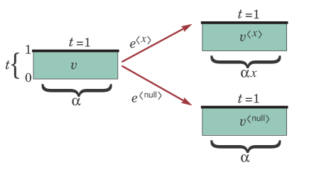
Figure 4.1. Atlas edges of two types:  $\operatorname{\text{\it e}}^{\langle x\rangle}=\bigl{(}\operatorname{{\text{\it\hskip 0.42677ptv}}},\operatorname{{\text{\it\hskip 0.42677ptv}}}^{\langle x\rangle}\bigr{)}$, where  $v=(\alpha,m,t)$  and  $\operatorname{{\text{\it\hskip 0.42677ptv}}}^{\langle x\rangle}=(\alpha x,m-1,1)$, and  $\operatorname{\text{\it e}}^{\langle\textsf{null}\rangle}=\bigl{(}\operatorname{{\text{\it\hskip 0.42677ptv}}},\operatorname{{\text{\it\hskip 0.42677ptv}}}^{\langle\textsf{null}\rangle}\bigr{)}$, where  $v=(\alpha,m,t)$  and  $\operatorname{{\text{\it\hskip 0.42677ptv}}}^{\langle\textsf{null}\rangle}=(\alpha,m-1,1)$.

For every word  $\alpha\in X^{*}$  of length  $\ell=|\alpha|$, and for every  $1\leq m\leq\textnormal{rk}(\mathscr{M})-\ell-1$, denote by  $\textbf{{A}}\hskip-0.85355pt{}(\alpha,m):=(\textrm{A}_{x\hskip 0.85355pty})_{x,y\in{\widehat{X}}}$  the symmetric  $\textnormal{d}\times\textnormal{d}$  matrix defined as follows:

(4.2) $$\ \begin{aligned} \ &\ \textrm{A}_{x\hskip 0.85355pty}\,:=\,\bigl{|}\operatorname{\textnormal{Cont}}_{m-1}(\alpha xy)\bigr{|}\qquad\text{for \ $x,y\in\operatorname{\textnormal{Cont}}(\alpha)$,}\\ \ &\ \textrm{A}_{x\hskip 1.70709pt\textsf{null}}\,=\,\textrm{A}_{\textsf{null}\hskip 1.70709ptx}\,:=\,\bigl{|}\operatorname{\textnormal{Cont}}_{m-1}(\alpha x)\bigr{|}\qquad\text{for \ \ $x\in\operatorname{\textnormal{Cont}}(\alpha)$,}\\ \ &\ \textrm{A}_{\textsf{null}\hskip 1.70709pt\textsf{null}}\,:=\,\bigl{|}\operatorname{\textnormal{Cont}}_{m-1}(\alpha)\bigr{|}\hskip 0.85355pt.\end{aligned}$$

For the first line, note that  $\textrm{A}_{x\hskip 0.85355pty}=\textrm{A}_{y\hskip 0.85355ptx}$  by matroid symmetry property. Note also that  $\textrm{A}_{x\hskip 0.85355ptx}=0$  for $x\in X$ since  $\alpha\beta xx$  is not simple. Next, observe that  $\textrm{A}_{x\hskip 0.85355pty}=0$  whenever  $x\notin\operatorname{\textnormal{Cont}}(\alpha)\cup\{\textsf{null}\}$  or  $y\notin\operatorname{\textnormal{Cont}}(\alpha)\cup\{\textsf{null}\}$. Finally, we have  $\textrm{A}_{x\hskip 1.70709pt\textsf{null}}>0$  whenever  $x\in\operatorname{\textnormal{Cont}}(\alpha)$, since by the exchange property the word  $\alpha x\in\operatorname{\mathcal{L}}$  can be extended to  $\alpha x\beta\in\operatorname{\mathcal{L}}$  for some  $\beta\in X^{*}$  with  $|\beta|\leq\textnormal{rk}(\mathscr{M})-\ell-1$.

For each vertex  $\operatorname{{\text{\it\hskip 0.42677ptv}}}=(\alpha,m,t)\in\operatorname{\Omega}$, define the associated matrix as follows:

$$\textbf{{M}}\hskip-0.85355pt{}\,=\,\textbf{{M}}\hskip-0.85355pt{}_{(\alpha,m,t)}\ :=\ t\,\textbf{{A}}\hskip-0.85355pt{}(\alpha,m+1)\ +\ (1-t)\,\textbf{{A}}\hskip-0.85355pt{}(\alpha,m).$$

Similarly, define the associated vector  $\operatorname{\mathbf{h}}=\operatorname{\mathbf{h}}_{(\alpha,m,t)}\in\operatorname{\mathbb{R}}^{\textnormal{d}}$  with coordinates

$$\textrm{h}_{x}\ :=\ \begin{cases}\,t&\text{ if }\ x\in X,\\ \,1-t&\text{ if }\ x=\textsf{null}.\end{cases}$$

Finally, define the linear transformation  $\mathbf{T}^{\langle x\rangle}:\operatorname{\mathbb{R}}^{\textnormal{d}}\to\operatorname{\mathbb{R}}^{\textnormal{d}}$  associated to the edge  $(\operatorname{{\text{\it\hskip 0.42677ptv}}},\operatorname{{\text{\it\hskip 0.42677ptv}}}^{\langle x\rangle})$ to be the identity map.

4.4. Properties of the atlas

We now show that our combinatorial atlas  $\mathbb{A}$  satisfies the conditions in Theorem 3.4, in the following series of lemmas.

Lemma 4.2.

For every vertex  $\operatorname{{\text{\it\hskip 0.42677ptv}}}\hskip 0.85355pt=\hskip 0.85355pt(\alpha,m,t)\in\operatorname{\Omega}$, we have:

1. the support  $\textnormal{supp}(\textbf{{\em M}}\hskip-0.85355pt{}_{\operatorname{{\text{\it\hskip 0.42677ptv}}}}\,)$  of the associated matrix  $\textbf{{\em M}}\hskip-0.85355pt{}_{\operatorname{{\text{\it\hskip 0.42677ptv}}}}$  is given by

   $$\textnormal{supp}\big{(}\textbf{{\em A}}\hskip-0.85355pt{}\,(\alpha,m+1)\big{)}\ =\ \textnormal{supp}\big{(}\textbf{{\em A}}\hskip-0.85355pt{}\,(\alpha,m)\big{)}\ =\ \begin{cases}\operatorname{\textnormal{Cont}}(\alpha)\hskip 0.85355pt\cup\hskip 0.85355pt\{{\textsf{\em null}}\}&\text{ if }\ \alpha\in\operatorname{\mathcal{L}}\\ \varnothing&\text{ if }\ \alpha\notin\operatorname{\mathcal{L}}\end{cases}$$

2. vertex  $\operatorname{{\text{\it\hskip 0.42677ptv}}}$  satisfies (Irr), and

3. vertex  $\operatorname{{\text{\it\hskip 0.42677ptv}}}$  satisfies (h-Pos)  for all  $t\in(0,1)$.

Proof.

Part (i) follows directly from the definition of matrices  M,  $\textbf{{A}}\hskip-0.85355pt{}(\alpha,m+1)$  and  $\textbf{{A}}\hskip-0.85355pt{}(\alpha,m)$. For part (ii), observe that if  $\alpha\notin\operatorname{\mathcal{L}}$, then M is a zero matrix and  $\operatorname{{\text{\it\hskip 0.42677ptv}}}$  trivially satisfies (Irr). On the other hand, if  $\alpha\in\operatorname{\mathcal{L}}$, then it follows from the definition of  $\textbf{{M}}\hskip-0.85355pt{}=\bigl{(}\textrm{M}_{x\hskip 0.85355pty}\bigr{)}$, that  $\textrm{M}_{x\hskip 1.70709pt\textsf{null}}>0$  for every  $x\in\operatorname{\textnormal{Cont}}(\alpha)$. Since the support of M  is  $\operatorname{\textnormal{Cont}}(\alpha)\hskip 0.85355pt\cup\hskip 0.85355pt\{\textsf{null}\}$, this proves (Irr). Finally, part (iii) follows from the fact that  $\operatorname{\mathbf{h}}_{\operatorname{{\text{\it\hskip 0.42677ptv}}}}$  is a strictly positive vector when  $t\in(0,1)$, and that M is a nonnegative matrix. ∎

Lemma 4.3.

For every matroid  $\mathscr{M}=(X,\operatorname{\mathcal{I}})$, the atlas  $\mathbb{A}$  satisfies (Inh).

Proof.

Let $\operatorname{{\text{\it\hskip 0.42677ptv}}}=(\alpha,m,t)\in\operatorname{\Omega}^{m}$, $m\geq 1$, be a non-sink vertex of $\operatorname{{\Gamma}}$. Let  $x\in{\widehat{X}}$. By the linearity of $\mathbf{T}^{\langle x\rangle}$, it suffices to show that for every  $y\in{\widehat{X}}$, we have:

$$\textrm{M}_{xy}\ =\ \big{\langle}\mathbf{T}^{\langle x\rangle}\operatorname{\mathbf{e}}_{y}\hskip 0.85355pt,\hskip 0.85355pt\textbf{{M}}\hskip-0.85355pt{}^{\langle x\rangle}\,\mathbf{T}^{\langle x\rangle}\operatorname{\mathbf{h}}\big{\rangle},$$

where  $\big{\{}\operatorname{\mathbf{e}}_{y},\hskip 1.70709pty\in{\widehat{X}}\big{\}}$  is the standard basis in  $\operatorname{\mathbb{R}}^{\textnormal{d}}$. We present only the proof for the case  $x,y\in\operatorname{\textnormal{Cont}}(\alpha)$, as the proof of the other cases are analogous.

First suppose that  $x,y\in\operatorname{\textnormal{Cont}}(\alpha)$  are distinct. Then:

$$\big{\langle}\mathbf{T}^{\langle x\rangle}\operatorname{\mathbf{e}}_{y}\hskip 0.85355pt,\hskip 0.85355pt\textbf{{M}}\hskip-0.85355pt{}^{\langle x\rangle}\,\mathbf{T}^{\langle x\rangle}\operatorname{\mathbf{h}}\big{\rangle}\quad=\ \ \sum_{z\hskip 0.85355pt\in\hskip 0.85355pt{\widehat{X}}}\textrm{M}^{\langle x\rangle}_{yz}\,\big{(}\mathbf{T}^{\langle x\rangle}\operatorname{\mathbf{h}}\big{)}_{z}\ =\ \sum_{z\hskip 0.85355pt\in\hskip 0.85355ptX}\,t\hskip 1.70709pt\textbf{{A}}\hskip-0.85355pt{}(\alpha x,m)_{yz}\ +\ (1-t)\hskip 1.70709pt\textbf{{A}}\hskip-0.85355pt{}(\alpha x,m)_{y\hskip 0.85355pt\textsf{null}}.$$

Let  $\ell:=|\alpha|$. By the definition of  $\textbf{{A}}\hskip-0.85355pt{}(\alpha x,m)$, this is equal to

(4.3) $$\begin{split}&\ \sum_{z\hskip 0.85355pt\in\hskip 0.85355ptX}\,t\,|\operatorname{\textnormal{Cont}}_{m-1}(\alpha xyz)|\ +\ (1-t)\,|\operatorname{\textnormal{Cont}}_{m-1}(\alpha xy)|\\ &\qquad\ =\ t\,|\operatorname{\textnormal{Cont}}_{m}(\alpha xy)|\ +\ (1-t)\,|\operatorname{\textnormal{Cont}}_{m-1}(\alpha xy)|.\end{split}$$

By the definition of  $\textbf{{A}}\hskip-0.85355pt{}(\alpha,m+1)$  and  $\textbf{{A}}\hskip-0.85355pt{}(\alpha,m)$, this is equal to

$$t\,\textbf{{A}}\hskip-0.85355pt{}(\alpha,m+1)_{xy}\ +\ (1-t)\,\textbf{{A}}\hskip-0.85355pt{}(\alpha,m)_{xy}\ =\ \textrm{M}_{xy}\hskip 1.70709pt,$$

which proves (Inh) for this case. This completes the proof. ∎

Lemma 4.4.

For every matroid  $\mathscr{M}=(X,\operatorname{\mathcal{I}})$, the atlas  $\mathbb{A}$  satisfies (T-Inv).

Proof.

Let $\operatorname{{\text{\it\hskip 0.42677ptv}}}=(\alpha,m,t)\in\operatorname{\Omega}^{m}$, $m\geq 1$, be a non-sink vertex of $\operatorname{{\Gamma}}$, and let  $x,y,z\in{\widehat{X}}$. We present only the proof of (T-Inv) for the case when  $x,y,z\in X$, as other cases follow analogously. We have:

(4.4) $$\textrm{M}_{yz}^{\langle x\rangle}\ =\ \textbf{{A}}\hskip-0.85355pt{}(\alpha x,m)_{yz}\ =\ |\operatorname{\textnormal{Cont}}_{m-1}(\alpha xyz)|\hskip 0.85355pt.$$

By the matroid symmetry property, the right side of the equation above is invariant under every permutation of $\{x,y,z\}$. This shows that  $\textrm{M}_{yz}^{\langle x\rangle}$  is invariant under every permutation of $\{x,y,z\}$, and the proof is complete. ∎

Lemma 4.5.

For every matroid  $\mathscr{M}=(X,\operatorname{\mathcal{I}})$, the atlas  $\mathbb{A}$  satisfies (DecSupp).

Proof.

Let $\operatorname{{\text{\it\hskip 0.42677ptv}}}=(\alpha,m,t)\in\operatorname{\Omega}^{m}$, $m\geq 1$, be a non-sink vertex of $\operatorname{{\Gamma}}$, and let $x\in{\widehat{X}}$. We need to show that  $\textnormal{supp}(\textbf{{M}}\hskip-0.85355pt{})\supseteq\textnormal{supp}(\textbf{{M}}\hskip-0.85355pt{}^{\langle x\rangle})$. First suppose that $\alpha\notin\operatorname{\mathcal{L}}$. Then by Lemma 4.2(i)  $\textnormal{supp}(\textbf{{M}}\hskip-0.85355pt{})=\textnormal{supp}\big{(}\textbf{{M}}\hskip-0.85355pt{}^{\langle x\rangle}\big{)}=\varnothing$, and the lemma hold trivially.

Now suppose that $\alpha\in\operatorname{\mathcal{L}}$. By Lemma 4.2(i), it suffices to show that  $\operatorname{\textnormal{Cont}}(\alpha)\supseteq\operatorname{\textnormal{Cont}}(\alpha x)$. Recall that for every  $\alpha xy\in\operatorname{\mathcal{L}}$  we have  $\alpha y\in\operatorname{\mathcal{L}}$  by the matroid symmetry and hereditary properties. This implies the result. ∎

4.5. Proof of Theorem 4.8

We first show that every sink vertex in  $\operatorname{{\Gamma}}$  is hyperbolic.

Lemma 4.6.

Let  $\mathscr{M}=(X,\operatorname{\mathcal{I}})$  be a matroid on  $|X|=n$ elements, and let  $1\leq k<\textnormal{rk}(\mathscr{M})$. Then every vertex in  $\operatorname{\Omega^{0}}$  satisfies (Hyp).

Proof.

Let  $\operatorname{{\text{\it\hskip 0.42677ptv}}}=(\alpha,0,1)\in\operatorname{\Omega^{0}}$  be a sink vertex, and let  $\ell:=|\alpha|$. It suffices to show that  $\textbf{{A}}\hskip-0.85355pt{}(\alpha,1)$  satisfies (Hyp). First note that if  $\alpha\notin\operatorname{\mathcal{L}}$, then  $\textbf{{A}}\hskip-0.85355pt{}(\alpha,1)$  is a zero matrix, and (Hyp) is trivially true. Thus, we can assume that  $\alpha\in\operatorname{\mathcal{L}}$. We write  $\textrm{A}_{x,y}\hskip 0.85355pt:=\hskip 0.85355pt\textbf{{A}}\hskip-0.85355pt{}(\alpha,1)_{xy}$  for every  $x,y\in X$.

We define an equivalence relation on $\operatorname{\textnormal{Cont}}(\alpha)$ by writing  $x\sim y$  if  $\alpha xy\not\in\operatorname{\mathcal{L}}$. Note that reflexivity of the relation follows from the fact that $\alpha xx$ is not a simple word, symmetry follows from the matroid symmetry property, and transitivity follows from the exchange property. Note that the number of equivalence classes  $r$  of this relation is at most

(4.5) $$r\ \leq\ |\operatorname{\textnormal{Cont}}(\alpha)|\ \leq\ n-\ell\ \leq\ n-k+1.$$

Now, for every  $x\in\textnormal{supp}(\textbf{{A}}\hskip-0.85355pt{})\setminus\{\textsf{null}\}$  and $y\in\textnormal{supp}(\textbf{{A}}\hskip-0.85355pt{})$, we have:

(4.6) $$\textrm{A}_{xy}\ =\ \begin{cases}1&\text{ if \hskip 1.70709pt$y\in X$ \hskip 1.70709ptand \hskip 1.70709pt$y\not\sim x$},\\ 0&\text{ if \hskip 1.70709pt$y\in X$ \hskip 1.70709ptand \hskip 1.70709pt$y\sim x$},\\ 1&\text{ if \hskip 1.70709pt$y=\textsf{null}$}.\end{cases}$$

In particular, this shows that the $x$-row (respectively, $x$-column) of  $\textbf{{A}}\hskip-0.85355pt{}(\alpha,1)$  is identical to the $y$-row (respectively, $y$-column) of  $\textbf{{A}}\hskip-0.85355pt{}(\alpha,1)$  whenever  $x\sim y$. In this case, deduct the $y$-row and $y$-column of  $\textbf{{A}}\hskip-0.85355pt{}(\alpha,1)$  by the $x$-row and $x$-column of  $\textbf{{A}}\hskip-0.85355pt{}(\alpha,1)$. It then follows from the claim that the resulting matrix has $y$-row and $y$-column is equal to zero. Note that (Hyp) is preserved under this transformation.

Now, apply the above linear transformation repeatedly, and by restricting to the support of resulting matrix. Since this preserves (Hyp), it suffices to prove that the following  $(r+1)\times(r+1)$  matrix satisfies (Hyp):

(4.7) $$\textbf{{B}}\hskip-0.85355pt{}\ =\ \begin{pmatrix}0&1&\hskip 3.0pt\cdots\hskip 3.0pt&1&1\\[2.0pt] 1&0&\cdots&1&1\\[2.0pt] \vdots&\vdots&\ddots&\vdots&\vdots\\[3.0pt] 1&1&\cdots&0&1\\[3.0pt] 1&1&\cdots&1&1\end{pmatrix}\hskip 0.85355pt.$$

Note that  B  has eigenvalue  $\lambda=-1$  with multiplicity $(r-1)$. Since  $\det(\textbf{{B}}\hskip-0.85355pt{})=(-1)^{r}$, we conclude that B has exactly one positive eigenvalue. By Lemma 3.5, this implies the result. ∎

We can now prove that every vertex in  $\operatorname{{\Gamma}}$  is hyperbolic.

Lemma 4.7.

Let  $\mathscr{M}=(X,\operatorname{\mathcal{I}})$  be a matroid on  $|X|=n$  elements, and let  $1\leq k<\textnormal{rk}(\mathscr{M})$. Then every vertex in  $\operatorname{\Omega}$  satisfies (Hyp).

Proof.

We induction on $m$ to show that every vertex in  $\operatorname{\Omega}^{m}$  satisfies (Hyp), for all  $m\leq k-1$. The claim is true for  $m=0$  by Lemma 4.6. Suppose that the claim is true for  $\operatorname{\Omega}^{m-1}$. Now note that the atlas  $\mathbb{A}$  satisfies all the necessary properties:  (Inh) by Lemma 4.3,  (T-Inv) by Lemma 4.4,  (DecSupp) by Lemma 4.5, and  (Iden) by definition. It then follows from Theorem 3.4 that every regular vertex in  $\operatorname{\Omega}^{m}$  satisfies (Hyp).

On the other hand, by Lemma 4.2, the regular vertices of  $\operatorname{\Omega}^{m}$  are those of the form  $\operatorname{{\text{\it\hskip 0.42677ptv}}}=(\alpha,m,t)$  with  $t\in(0,1)$. Since (Hyp) is preserved under taking the limits  $t\to 0$  and  $t\to 1$, it then follows that every vertex in $\operatorname{\Omega}^{m}$ satisfies (Hyp). This completes the proof. ∎

Proof of Theorem 4.1.

Let  $\textbf{{M}}\hskip-0.85355pt{}=\textbf{{M}}\hskip-0.85355pt{}_{\operatorname{{\text{\it\hskip 0.42677ptv}}}}$  be the matrix associated with the vertex  $\operatorname{{\text{\it\hskip 0.42677ptv}}}=(\varnothing,k-1,1)$. Let  $\operatorname{\mathbf{v}}$  and $\hskip 0.85355pt\operatorname{\mathbf{w}}$  be the characteristic vectors of  $X$  and  $\{\textsf{null}\}$, respectively. Then:

(4.8) $$\langle\operatorname{\mathbf{v}},\textbf{{M}}\hskip-0.85355pt{}\operatorname{\mathbf{v}}\rangle\ =\ (k+1)!\,\,{\textrm{I}}(k+1)\hskip 0.85355pt,$$

$$\langle\operatorname{\mathbf{v}},\textbf{{M}}\hskip-0.85355pt{}\operatorname{\mathbf{w}}\rangle\ =\ k!\,\hskip 1.70709pt{\textrm{I}}(k)\qquad\text{and}\qquad\langle\operatorname{\mathbf{w}},\textbf{{M}}\hskip-0.85355pt{}\operatorname{\mathbf{w}}\rangle\ =\ (k-1)!\,\hskip 1.70709pt{\textrm{I}}(k-1).$$

By Lemma 4.7, vertex  $\operatorname{{\text{\it\hskip 0.42677ptv}}}$  satisfies (Hyp). Substituting (4.8) into (Hyp), gives the inequality in the theorem. ∎

4.6. Ultra-log-concavity

In this section we extend the proof above to the obtain the strong Mason conjecture [Mas72], which was recently established independently by Anari et. al [ALOV18] and Brändén–Huh [BH20].

Theorem 4.8 (Ultra-log-concavity for matroids, [ALOV18, Thm 1.2] and [BH20, Thm 4.14], formerly strong Mason conjecture).

For a matroid  $\mathscr{M}=(X,\operatorname{\mathcal{I}})$,  $|X|=n$,  and integer  $1\leq k<\textnormal{rk}(\mathscr{M})$, we have:

(4.9) $${\text{\sc I}}(k)^{2}\,\geq\,\left(1\hskip 1.70709pt+\,\frac{1}{k}\right)\left(1\hskip 1.70709pt+\,\frac{1}{n-k}\right)\,\hskip 1.70709pt{\text{\sc I}}(k-1)\ {\text{\sc I}}(k+1)\hskip 0.85355pt.$$

Note that in [CP21], we used the same this proof technique to obtain an even stronger version of (4.9), see [CP21, §1.4] for details. In this paper we present only the proof of (4.9) for simplicity.

Proof of Theorem 4.8.

We proceed verbatim the proof above with minor changes. First, we modify the definition (4.2) of the symmetric  $\textnormal{d}\times\textnormal{d}$  matrix  $\textbf{{A}}\hskip-0.85355pt{}(\alpha,m)$  as follows:

$$\textrm{A}_{x\hskip 0.85355pty}\,:=\,c_{\ell+m+1}\,\bigl{|}\operatorname{\textnormal{Cont}}_{m-1}(\alpha xy)\bigr{|}\qquad\text{for \ $x,y\in\operatorname{\textnormal{Cont}}(\alpha)$,}$$

$$\textrm{A}_{x\hskip 1.70709pt\textsf{null}}\,=\,\textrm{A}_{\textsf{null}\hskip 1.70709ptx}\,:=\,c_{\ell+m}\,\bigl{|}\operatorname{\textnormal{Cont}}_{m-1}(\alpha x)\bigr{|}\qquad\text{for \ \ $x\in\operatorname{\textnormal{Cont}}(\alpha)$,}$$

$$\textrm{A}_{\textsf{null}\hskip 1.70709pt\textsf{null}}\,:=\,c_{\ell+m-1}\,\bigl{|}\operatorname{\textnormal{Cont}}_{m-1}(\alpha)\bigr{|},$$

where  $c_{i}:=1+\frac{1}{n-k}$  if  $i=k+1$, and  $c_{i}:=1$  otherwise. Then the intermediate equation (4.3) becomes

$$\begin{split}&\ \sum_{z\hskip 0.85355pt\in\hskip 0.85355ptX}\,t\,c_{\ell+m+2}\,|\operatorname{\textnormal{Cont}}_{m-1}(\alpha xyz)|\ +\ (1-t)\,c_{\ell+m+1}\,|\operatorname{\textnormal{Cont}}_{m-1}(\alpha xy)|\\ &\quad=\ t\,c_{\ell+m+2}\,|\operatorname{\textnormal{Cont}}_{m}(\alpha xy)|\ +\ (1-t)\,c_{\ell+m+1}\,|\operatorname{\textnormal{Cont}}_{m-1}(\alpha xy)|.\end{split}$$

but the conclusion of Lemma 4.3 remains valid.

Similarly, the equation (4.4) becomes

$$\textrm{M}_{yz}^{\langle x\rangle}\ =\ \textbf{{A}}\hskip-0.85355pt{}(\alpha x,m)_{yz}\ =\ c_{|\alpha|+m+2}\,|\operatorname{\textnormal{Cont}}_{m-1}(\alpha xyz)|\hskip 0.85355pt.$$

and the conclusion of Lemma 4.4 remains valid.

Finally, the proof of Lemma 4.6 is more technical in this case. First, the equation (4.6) becomes:

(4.10) $$\textrm{A}_{xy}\ =\ \begin{cases}c_{\ell+2}&\text{ if \hskip 1.70709pt$y\in X$ \hskip 1.70709ptand \hskip 1.70709pt$y\not\sim x$},\\ 0&\text{ if \hskip 1.70709pt$y\in X$ \hskip 1.70709ptand \hskip 1.70709pt$y\sim x$},\\ c_{\ell+1}&\text{ if \hskip 1.70709pt$y=\textsf{null}$}.\end{cases}$$

Next, matrix  B  in (4.7) is now

(4.11) $$\textbf{{B}}\hskip-0.85355pt{}\ =\ \begin{pmatrix}0&c_{\ell+2}&\hskip 3.0pt\cdots\hskip 3.0pt&c_{\ell+2}&c_{\ell+1}\\[2.0pt] c_{\ell+2}&0&&\vdots&\vdots\\[2.0pt] \vdots&&\ddots&c_{\ell+2}&c_{\ell+1}\\[3.0pt] c_{\ell+2}&\cdots&c_{\ell+2}&0&c_{\ell+1}\\[3.0pt] c_{\ell+1}&\ldots&c_{\ell+1}&c_{\ell+1}&c_{\ell}\end{pmatrix}.$$

Rescale the $i$-th row and $i$-th column ($i\leq r$) by  $\frac{1}{\sqrt{c_{\ell+2}}}$, and the $(r+1)$-th row and $(r+1)$-th column by $\frac{\sqrt{c_{\ell+2}}}{c_{\ell+1}}$. Note that (Hyp) is preserved under this transformation. The matrix becomes

$$\textbf{{B}}\hskip-0.85355pt{}^{\prime}\ =\ \begin{pmatrix}0&1&\hskip 3.0pt\cdots\hskip 3.0pt&1&1\\[2.0pt] 1&0&&\vdots&\vdots\\[2.0pt] \vdots&&\ddots&1&1\\[3.0pt] 1&\cdots&1&0&1\\[3.0pt] 1&\ldots&1&1&\frac{c_{\ell+2}\,c_{\ell}}{c_{\ell+1}^{2}}\end{pmatrix}.$$

By Lemma 3.5, it suffices to show that  $\textbf{{B}}\hskip-0.85355pt{}^{\prime}$  has exactly one positive eigenvalue. Indeed, observe that  $\lambda=-1$  is an eigenvalue of this matrix with multiplicity  $(r-1)$. So this matrix has exactly one positive eigenvalue if and only if the determinant of the matrix has sign  $(-1)^{r}$. On the other hand, the determinant of this matrix is equal to

$$(-1)^{r}\,\bigg{[}\frac{c_{\ell+2}\,c_{\ell}}{c_{\ell+1}^{2}}(1-r)+r\bigg{]}.$$

Now note that

$$\frac{c_{\ell+2}\,c_{\ell}}{c_{\ell+1}^{2}}\ =\ \left\{\begin{aligned} 1\qquad\ &\text{if \ \ $\ell<k-1$,}\\ 1+\frac{1}{n-k}\quad\ &\text{if \ \ $\ell=k-1$.}\end{aligned}\right.$$

In both cases, the determinant above has sign  $(-1)^{r}$  since  $r\leq n-k+1$  by (4.5). This completes the proof of Lemma 4.6 in this case ad finished the proof of property (Hyp).

Finally, in the proof of Theorem 4.8, equation (4.8) is modified as

(4.12) $$\langle\operatorname{\mathbf{v}},\textbf{{M}}\hskip-0.85355pt{}\operatorname{\mathbf{v}}\rangle\ =\ \left(1+\frac{1}{n-k}\right)\,(k+1)!\,\,{\textrm{I}}(k+1)\hskip 0.85355pt,$$

$$\langle\operatorname{\mathbf{v}},\textbf{{M}}\hskip-0.85355pt{}\operatorname{\mathbf{w}}\rangle\ =\ k!\,\hskip 1.70709pt{\textrm{I}}(k)\qquad\text{and}\qquad\langle\operatorname{\mathbf{w}},\textbf{{M}}\hskip-0.85355pt{}\operatorname{\mathbf{w}}\rangle\ =\ (k-1)!\,\hskip 1.70709pt{\textrm{I}}(k-1).$$

The rest of the proof is unchanged again. ∎

4.7. Abstract simplicial complex

An abstract simplicial complex is a pair $(X,\Delta)$, where $X$ is the ground set and  $\Delta\subseteq 2^{X}$  is a collection of subsets of $X$ that satisfies hereditary property:  $S\subset T$,  $T\in\Delta$   $\Rightarrow$   $S\in\Delta$ . The subsets in  $\Delta$  are called the faces of the simplicial complex. Note that a matroid is an abstract simplicial complex that additionally satisfies the exchange property. The rank of  $\Delta$, denoted by  $\textnormal{rk}(\Delta)$, is the largest cardinality of any of its faces. Note that the dimension $\dim(\Delta)$ of $\Delta$ is equal to $\textnormal{rk}(\Delta)-1$.

Let $k\in\{1,\ldots,\textnormal{rk}(\Delta)-1\}$. We now define the combinatorial atlas  $\mathbb{A}(\Delta,k)$  verbatim the same way combinatorial atlas for a matroid is defined in $\S$4.3. Note that the exchange property is never used in the definition, so when  $\Delta$  is a matroid  $\mathscr{M}$, the atlas  $\mathbb{A}(\Delta,k)$  is equal to the atlas  $\mathbb{A}(\mathscr{M},k)$.

Theorem 4.9.

Let  $\Delta$  be a simplicial complex. Suppose that every vertex in  $\mathbb{A}(\Delta,k)$  satisfies (Hyp), for all  $1\leq k<\textnormal{rk}(\Delta)$. Then  $\Delta$  is a matroid.

In other words, we show that the exchange property is necessary for the proof of Lemma 4.7, so Theorem 4.9 can be viewed as a converse to Lemma 4.7. The proof is based on he following quick calculation.

Lemma 4.10.

In conditions of the theorem, let  $U\in\Delta$, and let  $x\in X\setminus U$  such that  $U\cup\{x\}\in\Delta$. Then, for every distinct  $y,z\in X\setminus U$  such that  $U\cup\{y,z\}\in\Delta$, we have either  $U\cup\{x,y\}\in\Delta$  or  $U\cup\{x,z\}\in\Delta$.

Proof.

The claim is trivial when  $x=y$  or  $x=z$, so we can assume that  $x,y,z\in X\setminus U$  are all distinct. Let  $\alpha=x_{1}\ldots x_{\ell}\in\operatorname{\mathcal{L}}$  be any feasible word such that  $U=\{x_{1},\ldots,x_{\ell}\}$, and let $\textbf{{A}}\hskip-0.85355pt{}:=\textbf{{A}}\hskip-0.85355pt{}(\alpha,1)$. It follows from the assumption of the theorem that A satisfies (Hyp). Let $\textbf{{A}}\hskip-0.85355pt{}^{\prime}$ be the restriction of A to the rows and columns indexed by  $\{x,y,z,\textsf{null}\}$. Then  $\textbf{{A}}\hskip-0.85355pt{}^{\prime}$  also satisfies (Hyp). Now, suppose to the contrary that  $U\cup\{x,y\}\notin\Delta$  and  $U\cup\{x,z\}\notin\Delta$. Then

$$\textbf{{A}}\hskip-0.85355pt{}^{\prime}\ =\ \begin{bmatrix}0&0&0&1\\ 0&0&1&1\\ 0&1&0&1\\ 1&1&1&1\end{bmatrix}\qquad\text{ or }\qquad\textbf{{A}}\hskip-0.85355pt{}^{\prime}\ =\ \begin{bmatrix}0&0&0&1\\ 0&0&\frac{1}{n-1}&1\\ 0&\frac{1}{n-1}&0&1\\ 1&1&1&1\end{bmatrix},$$

where $n:=|X|>1$. In both cases, matrix  $\textbf{{A}}\hskip-0.85355pt{}^{\prime}$  has more than one positive eigenvalue. Now Lemma 3.5 gives a contradiction. ∎

Proof of Theorem 4.9.

Recall the statement of the exchange property:  for all  $S,T\in\Delta$  such that  $|S|<|T|$, there exists  $y\in T\setminus S$  such that  $S\cup\{y\}\in\Delta$. We this by induction on  $i:=|S\setminus T|$. The base case  $i=0$  is trivial, so suppose that  $i\geq 1$.

Let  $x\in S\setminus T$, and let  $U:=S\setminus x$. Since  $|U\setminus T|=i-1$, by the induction assumption there exists distinct  $y,z\in T\setminus U$  such that  $U\cup\{y,z\}\in\Delta$. By the lemma above, it then follows that either  $U\cup\{x,y\}\in\Delta$  or  $U\cup\{x,z\}\in\Delta$. By relabeling if necessary, we can assume that  $U\cup\{x,y\}\in\Delta$. Then we have  $S\cup\{y\}=U\cup\{x,y\}$, which proves the exchange property, as desired. ∎

5. Lorentzian polynomials

In this section we will show that the theory of Lorentzian polynomials introduced by Brändén and Huh in [BH20], can be expressed as a special case of our theory of the combinatorial atlas. We refer to the aforementioned paper for further references on this topic.

5.1. Background

Let  $n,\textnormal{r}\geq 0$  be nonnegative integers. We denote  $H_{n}^{\textnormal{r}}$  the set of degree r homogeneous polynomials in  $\operatorname{\mathbb{R}}[w_{1},\ldots,w_{n}]$. The Hessian of $f\in\operatorname{\mathbb{R}}[w_{1},\ldots,w_{n}]$ is the symmetric matrix

$$\operatorname{\mathscr{H}}_{f}(w)\ :=\ \big{(}\partial_{i}\partial_{j}f\big{)}_{i,j=1}^{n},$$

where $\partial_{i}$ stands for the partial derivative  $\frac{\partial}{\partial w_{i}}$.

For every $\operatorname{{\textbf{m}}}=(m_{1},\ldots,m_{n})\in\mathbb{N}^{n}$, we write

$$w^{\operatorname{{\textbf{m}}}}\ :=\ w_{1}^{m_{1}}\ldots w_{n}^{m_{n}}\quad\text{ and }\quad\partial^{\operatorname{{\textbf{m}}}}\ :=\ \partial_{1}^{\operatorname{{\textbf{m}}}_{1}}\ldots\partial_{n}^{\operatorname{{\textbf{m}}}_{n}}.$$

The r-th discrete simplex $\Delta_{n}^{\textnormal{r}}\subseteq\mathbb{N}^{n}$ is

$$\Delta_{n}^{\textnormal{r}}\ :=\ \bigl{\{}\operatorname{{\textbf{m}}}\in\mathbb{N}^{n}\,:\,m_{1}+\ldots+m_{n}=\textnormal{r}\bigr{\}}.$$

The support of a polynomial $f$ is the subset of $\mathbb{N}^{n}$ defined by

$$\textnormal{supp}(f)\ :=\ \{\operatorname{{\textbf{m}}}\in\mathbb{N}\,:\,\text{the coefficient of $w^{\operatorname{{\textbf{m}}}}$ in $f$ is nonzero}\}.$$

A subset $J\subseteq\mathbb{N}^{n}$ is M-convex if, for every $\operatorname{{\textbf{m}}},\operatorname{\mathbf{n}}\in J$ and every  $i\in[n]$  s.t. $m_{i}>n_{i}$, there exists  $j\in[n]$  s.t.   $m_{j}<n_{j}$  and  $\operatorname{{\textbf{m}}}-\operatorname{\mathbf{e}}_{i}+\operatorname{\mathbf{e}}_{j}\in J$, where $\operatorname{\mathbf{e}}_{1},\ldots,\operatorname{\mathbf{e}}_{n}$ is the standard basis in $\operatorname{\mathbb{R}}^{n}$.

Definition 5.1.

Let $f$ be a homogeneous polynomial of degree r with nonnegative coefficients. Then $f$ is Lorentzian if the support of $f$ is M-convex, and the Hessian of  $\partial^{\operatorname{{\textbf{m}}}}f$  has at most one positive eigenvalue, for every  $\operatorname{{\textbf{m}}}\in\Delta_{n}^{\textnormal{r}-2}$.

5.2. Combinatorial atlas for Lorentzian polynomials

In this section, we define a combinatorial atlas that arises naturally from Lorentzian polynomials. As a byproduct of this identification, we recover the following basic fact of Lorentzian polynomials.

Theorem 5.2 (cf. [BH20, Theorem 2.16(2)]).

Let $f$ be a Lorentzian polynomial. Then the Hessian of $f$ satisfies (Hyp) for every $(w_{1},\ldots,w_{n})\in\operatorname{\mathbb{R}}^{n}_{>0}$.

Let $f\in H_{n}^{\textnormal{r}}$ be a Lorentzian polynomial with $\textnormal{r}\geq 3$, and let $(w_{1},\ldots,w_{n})\in\operatorname{\mathbb{R}}^{n}_{>0}$. We define a combinatorial atlas  $\mathbb{A}:=\mathbb{A}(f,w_{1},\ldots,w_{n})$  as follows. Let  $\textnormal{d}:=n$  be the dimension of the atlas, and let  $X=[n]$. Let  $\operatorname{{\Gamma}}:=(\operatorname{\Omega},\operatorname{\Theta})$  be the acyclic digraph where the set of vertices  $\operatorname{\Omega}\hskip 0.85355pt:=\operatorname{\Omega^{0}}\cup\operatorname{\Omega}^{1}\cup\ldots\cup\operatorname{\Omega}^{\textnormal{r}-2}$  is given by

$$\operatorname{\Omega}^{m}\, :=\ \big{\{}\hskip 0.85355pt\alpha\in X^{*}\ :\ |\alpha|\hskip 0.85355pt=\hskip 0.85355pt\textnormal{r}-2-m\hskip 0.85355pt\big{\}},\quad\text{for}\ \ 0\leq m\leq\textnormal{r}-2\hskip 0.85355pt.$$

Each vertex  $\operatorname{{\text{\it\hskip 0.42677ptv}}}=\alpha\in\operatorname{\Omega}^{m}$,  $m\geq 1$, has exactly $n$ outgoing edges we label  $\bigl{(}\operatorname{{\text{\it\hskip 0.42677ptv}}},\operatorname{{\text{\it\hskip 0.42677ptv}}}^{\langle x\rangle}\bigr{)}\in\operatorname{\Theta}$, where  $\operatorname{{\text{\it\hskip 0.42677ptv}}}^{\langle x\rangle}=\alpha x$  for every  $x\in X$.

For each vertex  $\operatorname{{\text{\it\hskip 0.42677ptv}}}=\alpha$, where  $\alpha=x_{1}\hskip 0.85355pt\cdots\hskip 0.85355ptx_{\textnormal{r}-2-m}\in\operatorname{\Omega}^{m}$,  $m\geq 0$, define the associated matrix  $\textbf{{M}}\hskip-0.85355pt{}_{v}$  as follows:

$$\textbf{{M}}\hskip-0.85355pt{}_{v}\ :=\ \operatorname{\mathscr{H}}_{f}(\partial^{\alpha}w),\qquad\text{ where }\qquad\partial^{\alpha}\ :=\ \partial_{x_{1}}\ldots\partial_{x_{\textnormal{r}-2-m}}.$$

Define the associated vector  $\operatorname{\mathbf{h}}_{v}$  for $m\geq 1$, as follows:

$$\operatorname{\mathbf{h}}_{v}\ :=\ \,\Bigl{(}\frac{w_{1}}{m}\hskip 1.70709pt,\hskip 1.70709pt\ldots\hskip 1.70709pt,\hskip 1.70709pt\frac{w_{n}}{m}\Bigr{)}.$$

Finally, define the linear transformation  $\mathbf{T}^{\langle x\rangle}:\operatorname{\mathbb{R}}^{n}\to\operatorname{\mathbb{R}}^{n}$  associated to the edge  $\bigl{(}\operatorname{{\text{\it\hskip 0.42677ptv}}},\operatorname{{\text{\it\hskip 0.42677ptv}}}^{\langle x\rangle}\bigr{)}$, to be the identity map.

5.3. Proof of Theorem 5.2

We first verify that $\mathbb{A}$ satisfies all conditions in Theorem 3.4.

Lemma 5.3.

For every vertex  $\operatorname{{\text{\it\hskip 0.42677ptv}}}\hskip 0.85355pt=\hskip 0.85355pt\alpha\in\operatorname{\Omega}$, we have:

1. the support of the associated matrix  $\textbf{{\em M}}\hskip-0.85355pt{}_{\operatorname{{\text{\it\hskip 0.42677ptv}}}}$  is given by

   $$\textnormal{supp}(\textbf{{\em M}}\hskip-0.85355pt{}_{\operatorname{{\text{\it\hskip 0.42677ptv}}}}\,)\ =\ \bigl{\{}\hskip 0.85355pti\in[n]\,:\,\partial_{i}\partial^{\alpha}f\neq 0\hskip 0.85355pt\bigr{\}},$$

2. vertex  $\operatorname{{\text{\it\hskip 0.42677ptv}}}$  satisfies (Irr), and

3. vertex  $\operatorname{{\text{\it\hskip 0.42677ptv}}}\in\operatorname{\Omega}^{m}$  satisfies (h-Pos), for  $m\geq 1$.

Proof.

For part (i), note that $i\in[n]$ is not contained in  $\textnormal{supp}(\textbf{{M}}\hskip-0.85355pt{}_{v})$  if and only if  $\partial_{i}\partial_{j}\partial^{\alpha}f=0$  for every  $j\in[n]$ by definition. Since $f$ is a homogeneous polynomial with nonnegative coefficients, the latter is equivalent to $\partial_{i}\partial^{\alpha}f=0$, and the claim follows.

For part (ii), denote by  “$\sim$”  the equivalence relation on the support of  $\textbf{{M}}\hskip-0.85355pt{}=\textbf{{M}}\hskip-0.85355pt{}_{v}$, where two elements are equal if they are contained in the same irreducible component of M. Let us show that  $i\sim j$, for all  $i,j\in\textnormal{supp}(\textbf{{M}}\hskip-0.85355pt{})$. By part (i), there exist  $\operatorname{{\textbf{m}}},\operatorname{\mathbf{n}}\in\mathbb{N}^{n}$  in the support of $\partial^{\alpha}f$, such that  $\textrm{m}_{i}>0$  and  $\textrm{n}_{j}>0$.

Claim:  Every element $k$ in the support of  $\operatorname{{\textbf{m}}}$  satisfies  $k\sim i$.

Proof of Claim.

The claim is clear for  $k=i$, so suppose that  $k\neq i$. Then  $\partial_{i}\partial_{k}w^{\operatorname{{\textbf{m}}}}>0$. Since $\operatorname{{\textbf{m}}}$ is contained in the support of  $\partial^{\alpha}f$, this implies that $\textrm{M}_{ik}>0$, and the claim now follows. ∎

If  $\operatorname{{\textbf{m}}}=\operatorname{\mathbf{n}}$, then $i\sim j$ by the claim, so suppose to the contrary that  $\operatorname{{\textbf{m}}}\neq\operatorname{\mathbf{n}}$. Then there exists $k\in[n]$ such that  $\textrm{m}_{k}>\textrm{n}_{k}\geq 0$. Since $f$ is M-convex, there exists $\ell\in[n]$, such that  $\textrm{n}_{\ell}>\textrm{m}_{\ell}\geq 0$  and  $\operatorname{{\textbf{m}}}-\operatorname{\mathbf{e}}_{k}+\operatorname{\mathbf{e}}_{\ell}$  is contained in the support of $f$. We now show that  $i\sim\ell$. Indeed, If  $k\neq i$, then  $i\in\textnormal{supp}(\operatorname{{\textbf{m}}}-\operatorname{\mathbf{e}}_{k}+\operatorname{\mathbf{e}}_{\ell})$, which by the claim implies that $i\sim\ell$. If  $k=i$, then there exists  $h\in\textnormal{supp}(\operatorname{{\textbf{m}}}-\operatorname{\mathbf{e}}_{k})$  since the $\deg(w^{\operatorname{{\textbf{m}}}})=\deg(\partial^{\alpha}f)$ is at least 2. Then  $i\sim h$  and  $h\sim\ell$, by applying the claim to  $\operatorname{{\textbf{m}}}$  and  $\operatorname{{\textbf{m}}}-\operatorname{\mathbf{e}}_{k}+\operatorname{\mathbf{e}}_{\ell}$, respectively. By transitivity, we then have  $i\sim\ell$, as desired.

On the other hand, we have  $\ell\sim j$  by the claim applied to $\operatorname{\mathbf{n}}$. By transitivity, it then follows that  $i\sim j$, as desired. Since $i$ and $j$ are arbitrarily chosen, this shows that M is irreducible when restricted to its support, as desired.

Finally, part (iii) follows directly from the fact that $\operatorname{\mathbf{h}}_{v}$ is strictly positive by definition, and the fact that M is nonnegative. ∎

Lemma 5.4.

For every Lorentzian polynomial  $f$, the atlas  $\mathbb{A}$  satisfies (Inh), (T-Inv), (Iden), and (DecSupp).

Proof.

Let $\operatorname{{\text{\it\hskip 0.42677ptv}}}=\alpha\in\operatorname{\Omega}^{m}$, $m\geq 1$, be a non-sink vertex of $\operatorname{{\Gamma}}$. Note that (Iden) follows directly from definition. For (T-Inv), let  $i,j,k\in[n]$  be arbitrary elements. Then:

$$\textrm{M}^{(i)}_{jk}\ =\ \partial_{i}\partial_{j}\partial_{k}\partial^{\alpha}f,\quad\textrm{M}^{(j)}_{ki}\ =\ \partial_{j}\partial_{k}\partial_{i}\partial^{\alpha}f,\quad\textrm{M}^{(k)}_{ij}\ =\ \partial_{k}\partial_{i}\partial_{j}\partial^{\alpha}f,$$

which are all equal since partial derivatives commute with each other. This proves (T-Inv).

For (DecSupp), let  $i\in[n]$. By Lemma 5.3(i), the condition states that  $\partial_{j}\partial^{\alpha}f=0$  implies  $\partial_{j}\partial_{i}\partial^{\alpha}f=0$, for every $j\in[n]$. This is clear by commutativity again.

It remains to verify (Inh). First note that for every homogeneous polynomial  $g$  of degree  $m\geq 1$, we have:

(5.1) $$g\ =\ \frac{1}{m}\hskip 1.70709pt\sum_{i=1}^{n}\hskip 1.70709ptw_{i}\hskip 0.85355pt\partial_{i}g.$$

Let  $i\in[n]$  and  $\operatorname{\mathbf{v}}\in\operatorname{\mathbb{R}}^{n}$. We have:

$$\big{\langle}\mathbf{T}^{\langle i\rangle}\operatorname{\mathbf{v}},\,\textbf{{M}}\hskip-0.85355pt{}^{\langle i\rangle}\,\mathbf{T}^{\langle i\rangle}\operatorname{\mathbf{h}}\big{\rangle}\ =_{\eqref{eq:Iden}}\big{\langle}\operatorname{\mathbf{v}},\,\textbf{{M}}\hskip-0.85355pt{}^{\langle i\rangle}\,\operatorname{\mathbf{h}}\big{\rangle}\ =\ \sum_{j=1}^{n}\hskip 1.70709pt\sum_{k=1}^{n}\hskip 1.70709pt\textrm{v}_{j}\hskip 1.70709pt\frac{w_{k}}{m}\,\partial_{j}\partial_{k}\partial_{i}\partial^{\alpha}f$$

$$\qquad=\ \sum_{j=1}^{n}\hskip 1.70709pt\textrm{v}_{j}\hskip 1.70709pt\frac{1}{m}\hskip 1.70709pt\sum_{k=1}^{n}\hskip 1.70709ptw_{k}\,\partial_{k}\,\Bigl{(}\partial_{i}\partial_{j}\partial^{\alpha}f\Bigr{)}\ =_{\eqref{eqmike 1}}\ \sum_{j=1}^{k}\hskip 1.70709pt\textrm{v}_{j}\,\partial_{j}\partial_{i}\partial^{\alpha}f\ =\ \big{(}\textbf{{M}}\hskip-0.85355pt{}\operatorname{\mathbf{v}}\big{)}_{i}\hskip 1.70709pt.$$

This proves (Inh). ∎

Proof of Theorem 5.2.

Note that the atlas $\mathbb{A}$ satisfies every condition of Theorem 3.4 by Lemma 5.4. Note also that every non-sink vertex of $\mathbb{A}$ is regular by Lemma 5.3. Applying Theorem 3.4 iteratively, it suffices to show that the Hessian of  $\partial^{\alpha}f$  satisfies (Hyp) for every  $|\alpha|=\textnormal{r}-2$. However, this is the assumption of Lorentzian polynomial, and the theorem now follows. ∎

6. Alexandrov–Fenchel inequality

In this section we give an elementary self-contained proof of the classical Alexandrov–Fenchel inequality. As we mentioned in the introduction, despite the difference in presentation, the heart of the argument follows the proof in [SvH19, Thm 5.2] combined with a few geometric arguments based on the presentation in [Sch14].

6.1. Mixed volumes

Fix  $n\geq 1$. For two sets  $A,B\subset\operatorname{\mathbb{R}}^{n}$  and constants  $a,b>0$, denote by

$$aA+bB\ :=\ \bigl{\{}\hskip 0.85355pta\operatorname{\mathbf{x}}+b\operatorname{\mathbf{y}}\,:\,\operatorname{\mathbf{x}}\in A,\operatorname{\mathbf{y}}\in B\hskip 0.85355pt\bigr{\}}$$

the Minkowski sum of these sets. For a convex body  $K\subset\operatorname{\mathbb{R}}^{n}$, denote by  $\textnormal{Vol}_{n}(K)$  the volume of $K$. One of the basic result in convex geometry is Minkowski’s theorem that the volume of convex bodies in $\operatorname{\mathbb{R}}^{n}$ behaves as a homogeneous polynomial of degree $n$ with nonnegative coefficients:

Theorem 6.1 (Minkowski, see e.g. [BuZ88, $\S$19.1]).

For all convex bodies  $\textnormal{K}_{1},\ldots,\textnormal{K}_{r}\subset\operatorname{\mathbb{R}}^{n}$  and  $\lambda_{1},\ldots,\lambda_{r}>0$, we have:

(6.1) $$\textnormal{Vol}_{n}(\lambda_{1}\textnormal{K}_{1}+\ldots+\lambda_{r}\textnormal{K}_{r})\ =\ \sum_{1\hskip 0.85355pt\leq\hskip 0.85355pti_{1}\hskip 0.85355pt,\hskip 0.85355pt\ldots\hskip 0.85355pt,\hskip 0.85355pti_{n}\hskip 0.85355pt\leq\hskip 0.85355ptr}\hskip 1.70709pt\textnormal{V}\bigl{(}\textnormal{K}_{i_{1}},\ldots,\textnormal{K}_{i_{n}}\bigr{)}\,\lambda_{i_{1}}\hskip 0.85355pt\cdots\hskip 0.85355pt\lambda_{i_{n}},$$

where the functions  $\textnormal{V}(\cdot)$  are nonnegative and symmetric.

The coefficients  $\textnormal{V}(\textnormal{K}_{i_{1}},\ldots,\textnormal{K}_{i_{n}})$  are called mixed volumes of  $\textnormal{K}_{i_{1}},\ldots,\textnormal{K}_{i_{n}}$. They are invariant under translations:

$$\textnormal{V}(\textnormal{K}_{1}+\textbf{{a}}_{1},\ldots,\textnormal{K}_{n}+\textbf{{a}}_{n})\ =\ \textnormal{V}(\textnormal{K}_{1},\ldots,\textnormal{K}_{n})\quad\,\text{for every \ \hskip 1.70709pt$\textbf{{a}}_{1},\ldots,\textbf{{a}}_{n}\in\operatorname{\mathbb{R}}^{n}$.}$$

From this point on, every convex body in this section is assumed to be equivalent under translations. Note also that  $\textnormal{V}(\textnormal{K},\ldots,\textnormal{K})=\textnormal{Vol}_{n}(\textnormal{K})$  for every convex body  $K\subset\operatorname{\mathbb{R}}^{n}$, and that  $\textnormal{V}(\cdot)$  is multilinear:

$$\textnormal{V}(\lambda\textnormal{K}+\lambda^{\prime}\textnormal{K}^{\prime},\textnormal{K}_{2},\ldots,\textnormal{K}_{n})\ =\ \lambda\hskip 1.70709pt\textnormal{V}(\textnormal{K},\textnormal{K}_{2},\ldots,\textnormal{K}_{n})\hskip 1.70709pt+\hskip 1.70709pt\lambda^{\prime}\hskip 1.70709pt\textnormal{V}(\textnormal{K}^{\prime},\textnormal{K}_{2},\ldots,\textnormal{K}_{n})\quad\text{for every \ $\lambda,\lambda^{\prime}>0$.}$$

Finally, mixed volumes are monotone:

$$\textnormal{V}(\textnormal{K}_{1},K_{2},\ldots,\textnormal{K}_{n})\,\geq\,\textnormal{V}(\textnormal{K}_{1}^{\prime},\textnormal{K}^{\prime}_{2},\ldots,\textnormal{K}^{\prime}_{n})\quad\text{for all}\ \ \textnormal{K}_{i}\supseteq\textnormal{K}_{i}^{\prime}\hskip 1.70709pt,\ 1\leq i\leq n.$$

We will not prove Minkowski’s theorem which is elementary and well presented in a number of textbooks, such as [Ale50, $\S$8.3], [BuZ88, $\S$19.1], [Sch14, $\S$5.1], and most recently in [HG20, $\S$3.3]. Instead, we will be concerned with the following classical inequality:

Theorem 6.2 (Alexandrov–Fenchel inequality, see e.g. [BjZ92, $\S$20] ).

For convex bodies  A, B, $\textnormal{K}_{1}$,  $\ldots$  , $\textnormal{K}_{n-2}\subset\operatorname{\mathbb{R}}^{n}$, we have:

(AF) $$\textnormal{V}(\textnormal{A},\textnormal{B},\textnormal{K}_{1},\ldots,\textnormal{K}_{n-2})^{2}\ \geq\ \textnormal{V}(\textnormal{A},\textnormal{A},\textnormal{K}_{1},\ldots,\textnormal{K}_{n-2})\hskip 1.70709pt\cdot\hskip 1.70709pt\textnormal{V}(\textnormal{B},\textnormal{B},\textnormal{K}_{1},\ldots,\textnormal{K}_{n-2}).$$

The way our proof works is by establishing hyperbolicity of a certain matrix (Theorem 6.15), which is where our combinatorial atlas technology comes in. Unfortunately, both the matrix and the proof emerge in the middle of a technical calculations some of which are standard, which go back to Minkowski and Alexandrov, and are widely available in the literature. In an effort to make the proof self-contained, we made a choice to include them all, sticking as much as possible to the presentation in Chapters 2 and 5 of [Sch14].

6.2. Mixed volume preliminaries

In this section we collect basic properties of mixed volumes that will be used in the proof of Theorem 6.2. The reader well versed with mixed volumes can skip this subsection.

Let  $\textnormal{W}\subseteq\operatorname{\mathbb{R}}^{n}$  be a linear subspace of dimension  $\dim(\textnormal{W})=m\geq 1$. All polytopes in this paper are assumed to be convex. A convex polytope  $P\subset W$  is called $m$-dimensional if it has nonempty interior. An $m$-dimensional polytope $\textnormal{P}\subset\textnormal{W}$ is simple if each vertex is contained in exactly $m$ facets. The following easy lemma proves positivity of mixed volumes of simple polytopes.

Lemma 6.3 (cf. [Sch14, Thm 5.1.8]).

Let  $\textnormal{P}_{1},\ldots,\textnormal{P}_{m}\subset\textnormal{W}$  be convex $m$-dimensional polytopes. Then  $\textnormal{V}(\textnormal{P}_{1},\ldots,\textnormal{P}_{m})>0$.

Proof.

Since $\textnormal{P}_{1},\ldots,\textnormal{P}_{m}$ are $m$-dimensional, there exists line segments  $\textnormal{S}_{i}\subset\textnormal{P}_{i}$ ,  $1\leq i\leq m$, such that  $\textnormal{S}_{1},\ldots,\textnormal{S}_{m}$  span W. By the monotonicity of mixed volumes, we have:

$$\textnormal{V}(\textnormal{P}_{1},\ldots,\textnormal{P}_{m})\ \geq\ \textnormal{V}(\textnormal{S}_{1},\ldots,\textnormal{S}_{m}).$$

On the other hand, by direct calculation, we have:

$$\textnormal{V}(\textnormal{S}_{1},\ldots,\textnormal{S}_{m})\ =\ \frac{1}{m!}\,\textnormal{Vol}_{m}(\textnormal{S}_{1}+\ldots+\textnormal{S}_{m})\ >\ 0.$$

since  $\textnormal{S}_{1}+\ldots+\textnormal{S}_{m}$  is an $m$-dimensional parallelepiped with positive volume. ∎

Denote by  $\textnormal{F}(\textnormal{P},\operatorname{\mathbf{u}})$  the face of the polytope P with normal direction  $\operatorname{\mathbf{u}}\in\operatorname{\mathbb{S}}^{n-1}$. We say that polytopes  $\textnormal{P},\textnormal{P}^{\prime}\subset\textnormal{W}$  are strongly isomorphic if

$$\dim\textnormal{F}(\textnormal{P},\operatorname{\mathbf{u}})\ =\ \dim\textnormal{F}(\textnormal{P}^{\prime},\operatorname{\mathbf{u}})\quad\text{ for all }\operatorname{\mathbf{u}}\in\operatorname{\mathbb{S}}^{n-1}\hskip 0.85355pt\cap\hskip 0.85355pt\textnormal{W}.$$

This is a very strong condition which implies that polytopes P and $\textnormal{P}^{\prime}$ are combinatorially equivalent (have isomorphic face lattices), with the corresponding faces parallel to each other. Being strongly isomorphic is an equivalence relation on polytopes in W, and the equivalence classes of this relation are called $a$-types.

For the rest of this section, let  $\operatorname{\mathcal{A}}$  be a fixed $a$-type of W. Let  $\operatorname{\mathbf{u}}^{\langle 1\rangle},\operatorname{\mathbf{u}}^{\langle 2\rangle},\ldots$  be the unit vectors in W normals to facets of polytopes in $\operatorname{\mathcal{A}}$, so we have:

$$\dim\textnormal{F}\big{(}\textnormal{P},\operatorname{\mathbf{u}}^{\langle i\rangle}\big{)}\ =\ m-1\quad\text{ for all }\ \textnormal{P}\in\operatorname{\mathcal{A}}.$$

Denote by  $\textnormal{W}^{\langle i\rangle}$  the hyperplane in W that contains the origin  ${\mathbf{0}}\in\textnormal{W}$, and is orthogonal to  $\operatorname{\mathbf{u}}^{\langle i\rangle}.$

For a polytope  $\textnormal{P}\in\operatorname{\mathcal{A}}$, the support vector  $\operatorname{\mathbf{h}}_{\textnormal{P}}\in\operatorname{\mathbb{R}}^{\textnormal{d}}$  is given by

$$\big{(}\operatorname{\mathbf{h}}_{\textnormal{P}}\big{)}_{i}\ :=\ \sup_{\operatorname{\mathbf{x}}\in\textnormal{P}}\ \langle\operatorname{\mathbf{u}}^{\langle i\rangle},\operatorname{\mathbf{x}}\rangle,$$

the distance to the origin ${\mathbf{0}}$ of the supporting hyperplane of P whose normal direction is $\operatorname{\mathbf{u}}^{\langle i\rangle}$. Note that the polytope  $\textnormal{P}\in\operatorname{\mathcal{A}}$  is uniquely determined by the support vector  $\operatorname{\mathbf{h}}_{\textnormal{P}}$. Note also that  $\operatorname{\mathbf{h}}_{\textnormal{P}}$  is strictly positive if and only if ${\mathbf{0}}$ is contained in the interior of  P. Finally, note that support vectors convert Minkowski sum into scalar sum, i.e.  $\operatorname{\mathbf{h}}_{a\textnormal{A}+b\textnormal{B}}\hskip 1.70709pt=\hskip 1.70709pta\operatorname{\mathbf{h}}_{\textnormal{A}}\hskip 0.85355pt+\hskip 1.70709ptb\operatorname{\mathbf{h}}_{\textnormal{B}}$  for all  $a,b\geq 0$.

The next lemma shows that every vector in  $\operatorname{\mathbb{R}}^{\textnormal{d}}$  can be expressed as a linear combination of support vectors.

Lemma 6.4 (cf. [Sch14, Lem. 2.4.13]).

Let  $\textnormal{P}\in\operatorname{\mathcal{A}}$  be a simple polytope. Then there exists  $\varepsilon>0$, such that for every  $\operatorname{\mathbf{v}}\in\operatorname{\mathbb{R}}^{\textnormal{d}}$  with $|\operatorname{\mathbf{v}}|<\varepsilon$, we have:

$$\operatorname{\mathbf{v}}\ =\ \operatorname{\mathbf{h}}_{\textnormal{Q}}-\operatorname{\mathbf{h}}_{\textnormal{P}}\hskip 0.85355pt,$$

for some simple polytope  $\textnormal{Q}\in\operatorname{\mathcal{A}}$  strongly isomorphic to P.

Proof.

Let

$$\textnormal{Q}\ :=\ \bigl{\{}\hskip 1.70709pt\operatorname{\mathbf{x}}\in\textnormal{W}\,:\,\langle\operatorname{\mathbf{u}}^{\langle i\rangle},\operatorname{\mathbf{x}}\rangle\leq\big{(}\operatorname{\mathbf{h}}_{\textnormal{P}}+\operatorname{\mathbf{v}}\big{)}_{i}\ \text{ for every }i\in[\textnormal{d}]\hskip 1.70709pt\bigr{\}}$$

be a polytope formed by translating the supporting hyperplanes of P. Note that the property of being simple and being contained in $\operatorname{\mathcal{A}}$ is preserved under small enough pertubations. The conclusion of the lemma now follows. ∎

For every distinct  $i,j\in[\textnormal{d}]$ , denote by  $\theta^{\langle ij\rangle}\in[0,\pi]$  the angle between $\operatorname{\mathbf{u}}^{\langle i\rangle}$ and $\operatorname{\mathbf{u}}^{\langle j\rangle}$, so we have  $\cos\theta^{\langle ij\rangle}\hskip 1.70709pt=\hskip 1.70709pt\big{\langle}\operatorname{\mathbf{u}}^{\langle i\rangle},\operatorname{\mathbf{u}}^{\langle j\rangle}\big{\rangle}$. Let  $\textnormal{P}_{1},\ldots,\textnormal{P}_{r}\in\operatorname{\mathcal{A}}$  be simple, strongly isomorphic polytopes. For every  $k\in[r]$, we write

(6.2) $$\textnormal{F}_{k}^{\langle i\rangle}\ :=\ \textnormal{F}\big{(}\textnormal{P}_{k},\operatorname{\mathbf{u}}^{\langle i\rangle}\big{)}\quad\text{and}\quad\textnormal{F}_{k}^{\langle ij\rangle}\ :=\ \textnormal{F}_{k}^{\langle i\rangle}\cap\textnormal{F}_{k}^{\langle j\rangle},$$

for the faces of $\textnormal{P}_{k}$ that corresponds to the normal direction  $\operatorname{\mathbf{u}}^{\langle i\rangle}$  and for the pair of directions  $\bigl{\{}\operatorname{\mathbf{u}}^{\langle i\rangle},\operatorname{\mathbf{u}}^{\langle j\rangle}\bigr{\}}$, respectively. By definition, we have  $\theta^{\langle ij\rangle}=\theta^{\langle ji\rangle}$  and  $\textnormal{F}_{k}^{\langle ij\rangle}\hskip 1.70709pt=\hskip 1.70709pt\textnormal{F}_{k}^{\langle ji\rangle}$. When  $r=1$, i.e. there is only one polytope  $\textnormal{P}=\textnormal{P}_{1}$, we omit subscript $1$ from the notation.

The next lemma show that the properties of being simple and strongly isomorphic are inherited by the facets of the polytopes.

Lemma 6.5 (cf. [Sch14, Lemma 2.4.10]).

Let  $\textnormal{P}_{1},\textnormal{P}_{2}\in\operatorname{\mathcal{A}}$  be simple strongly isomorphic $m$-dimensional polytopes. Suppose  $\textnormal{F}_{1}$  and  $\textnormal{F}_{2}$  are facets of  $\textnormal{P}_{1}$  and $\textnormal{P}_{2}$  corresponding to the same normal direction. Then  $\textnormal{F}_{1}$  and  $\textnormal{F}_{2}$  are simple, strongly isomorphic $(m-1)$-dimensional polytopes.

Proof.

The case $m=1$ is trivial, so we assume that $m\geq 2$. By definition, the facets of a simple $m$-dimensional polytope are again simple $(m-1)$-dimensional polytopes. It thus suffices to show that  $\textnormal{F}_{1}$  and  $\textnormal{F}_{2}$  are strongly isomorphic polytopes. Let  $\textnormal{F}_{1}^{\prime}$  and  $\textnormal{F}_{2}^{\prime}$  be faces of  $\textnormal{F}_{1}$  and  $\textnormal{F}_{2}$  with the same unit normal direction. Then there exists  $\operatorname{\mathbf{u}}\in\operatorname{\mathbb{S}}^{n-1}$, such that  $\textnormal{F}_{1}^{\prime}$  and  $\textnormal{F}_{2}^{\prime}$  are faces of  $\textnormal{P}_{1}$  and  $\textnormal{P}_{2}$  with the normal direction $\operatorname{\mathbf{u}}$. Since  $\textnormal{P}_{1}$  and  $\textnormal{P}_{2}$  are strongly isomorphic, it then follows that

$$\dim\textnormal{F}_{1}^{\prime}\ =\ \dim\hskip 0.85355pt\textnormal{F}(\textnormal{P}_{1},\operatorname{\mathbf{u}})\ =\ \dim\hskip 0.85355pt\textnormal{F}(\textnormal{P}_{2},\operatorname{\mathbf{u}})\ =\ \dim\textnormal{F}_{2}^{\prime}\hskip 1.70709pt,$$

as desired. ∎

Now let  $m\geq 2$, let  $\textnormal{P}\in\operatorname{\mathcal{A}}$  be a simple polytope, and and let  $\textnormal{J}=\textnormal{J}(\operatorname{\mathcal{A}})$  be given by

$$\textnormal{J}\ :=\ \bigl{\{}\hskip 0.85355pt(i,j)\in[\textnormal{d}]^{2}\ \ \ \text{s.t.}\ \ \dim\textnormal{F}^{\langle ij\rangle}\ =\ m-2\bigr{\}}.$$

Note that  J  does not depend on the choice of  $\textnormal{P}\in\operatorname{\mathcal{A}}$  since the facets of polytopes in  $\operatorname{\mathcal{A}}$  are strongly isomorphic by Lemma 6.5. Also note that  $\theta^{\langle ij\rangle}\notin\{0,\pi\}$  for all  $(i,j)\in\textnormal{J}$, so both  $\csc\theta^{\langle ij\rangle}$  and  $\cot\theta^{\langle ij\rangle}$  are well defined.

The next lemma relates the support vector of a polytope to the support vector of its facets.

Lemma 6.6 (cf. [Sch14, Eq. (5.4)]).

Let $m\geq 2$, let  $\textnormal{P}\in\operatorname{\mathcal{A}}$  be an $m$-dimensional polytope. Then, for all $(i,j)\in\textnormal{J}$,

$$\big{(}\operatorname{\mathbf{h}}_{\textnormal{F}^{\langle i\rangle}}\big{)}_{j}\ =\ \big{(}\operatorname{\mathbf{h}}_{\textnormal{P}}\big{)}_{j}\csc\theta^{\langle ij\rangle}\ -\ \big{(}\operatorname{\mathbf{h}}_{\textnormal{P}}\big{)}_{i}\cot\theta^{\langle ij\rangle}.$$

Proof.

Let  $\operatorname{\mathbf{u}}^{\langle ij\rangle}\perp\operatorname{\mathbf{u}}^{\langle i\rangle}$  be the unit normal vector of the $(m-1)$-polytope  $\textnormal{F}^{\langle i\rangle}$  at its $(m-2)$-face  $\textnormal{F}^{\langle ij\rangle}$. Note that

$$\operatorname{\mathbf{u}}^{\langle j\rangle}\ =\ \operatorname{\mathbf{u}}^{\langle i\rangle}\hskip 1.70709pt\cos\theta^{\langle ij\rangle}\ +\ \operatorname{\mathbf{u}}^{\langle ij\rangle}\hskip 1.70709pt\sin\theta^{\langle ij\rangle}.$$

This implies that

(6.3) $$\big{(}\operatorname{\mathbf{h}}_{\textnormal{F}^{\langle i\rangle}}\big{)}_{j}\ =\ \sup_{\operatorname{\mathbf{x}}\in\textnormal{F}^{\langle i\rangle}}\langle\operatorname{\mathbf{u}}^{\langle ij\rangle},\operatorname{\mathbf{x}}\rangle\ =\ \sup_{\operatorname{\mathbf{x}}\in\textnormal{F}^{\langle i\rangle}}\langle\operatorname{\mathbf{u}}^{\langle j\rangle},\operatorname{\mathbf{x}}\rangle\hskip 1.70709pt\csc\theta^{\langle ij\rangle}\ -\ \langle\operatorname{\mathbf{u}}^{\langle i\rangle},\operatorname{\mathbf{x}}\rangle\hskip 1.70709pt\cot\theta^{\langle ij\rangle}.$$

On the other hand, we have

(6.4) $$\sup_{\operatorname{\mathbf{x}}\in\textnormal{F}^{\langle i\rangle}}\langle\operatorname{\mathbf{u}}^{\langle j\rangle},\operatorname{\mathbf{x}}\rangle\ =\ \big{(}\operatorname{\mathbf{h}}_{\textnormal{P}}\big{)}_{j}\qquad\text{ and }\qquad\langle\operatorname{\mathbf{u}}^{\langle i\rangle},\operatorname{\mathbf{x}}\rangle\ =\ \big{(}\operatorname{\mathbf{h}}_{\textnormal{P}}\big{)}_{i}\ \ \text{ for all }\operatorname{\mathbf{x}}\in\textnormal{F}^{\langle i\rangle},$$

where the first equality hold because we have  $\textnormal{F}^{\langle i\rangle}\cap\textnormal{F}^{\langle j\rangle}\neq\varnothing$  by the assumption that  $(i,j)\in\textnormal{J}$. The lemma now follows by combining equations (6.3) and (6.4). ∎

The next lemma relates the volume of a polytope to the volumes of its facets.

Lemma 6.7 (cf. [Sch14, Lemma 5.1.1]).

Let  $\textnormal{P}\in\operatorname{\mathcal{A}}$  be an $m$-dimensional polytope. Then

(6.5) $$\textnormal{Vol}_{m}(\textnormal{P})\ =\ \frac{1}{m}\hskip 1.70709pt\sum_{i=1}^{\textnormal{d}}\hskip 1.70709pt\big{(}\operatorname{\mathbf{h}}_{\textnormal{P}}\big{)}_{i}\hskip 1.70709pt\textnormal{Vol}_{m-1}\big{(}\textnormal{F}^{\langle i\rangle}\big{)}.$$

Proof.

The case $m=1$ is trivial, so we assume that $m\geq 2$. We first show that

(6.6) $$\sum_{i=1}^{\textnormal{d}}\hskip 1.70709pt\textnormal{Vol}_{m-1}\big{(}\textnormal{F}^{\langle i\rangle}\big{)}\hskip 1.70709pt\operatorname{\mathbf{u}}^{\langle i\rangle}\ =\ {\mathbf{0}}.$$

Let  $\operatorname{\mathbf{z}}\in\textnormal{W}\cap\operatorname{\mathbb{S}}^{n-1}$  be an arbitrary unit vector in  W, and let  $\textnormal{P}^{\prime}$  be the orthogonal projection of  P  onto  $\operatorname{\mathbf{z}}^{\perp}$. Then:

$$\textnormal{Vol}_{m-1}(\textnormal{P}^{\prime})\ =\ \sum_{\langle\operatorname{\mathbf{z}},\operatorname{\mathbf{u}}^{\langle i\rangle}\rangle\geq 0}\hskip 1.70709pt\langle\operatorname{\mathbf{z}},\operatorname{\mathbf{u}}^{\langle i\rangle}\rangle\,\textnormal{Vol}_{m-1}\big{(}\textnormal{F}^{\langle i\rangle}\big{)}\ =\ -\sum_{\langle\operatorname{\mathbf{z}},\operatorname{\mathbf{u}}^{\langle i\rangle}\rangle<0}\hskip 1.70709pt\langle\operatorname{\mathbf{z}},\operatorname{\mathbf{u}}^{\langle i\rangle}\rangle\,\textnormal{Vol}_{m-1}\big{(}\textnormal{F}^{\langle i\rangle}\big{)}.$$

This implies that

$$\sum_{i=1}^{\textnormal{d}}\hskip 1.70709pt\langle\operatorname{\mathbf{z}},\operatorname{\mathbf{u}}^{\langle i\rangle}\rangle\,\textnormal{Vol}_{m-1}\big{(}\textnormal{F}^{\langle i\rangle}\big{)}\ =\ 0.$$

Since  $\operatorname{\mathbf{z}}$  is arbitrary, the equation (6.6) follows.

From (6.6), we see that the right side of (6.5) does not change under translations of P. Since this is also true for the left side of (6.5), we may assume that the origin ${\mathbf{0}}$ is contained in the interior of P. Then  P  is the union of the pyramids  $\text{conv}\big{(}\textnormal{F}^{\langle i\rangle}\cup\{{\mathbf{0}}\}\big{)}$,  $1\leq i\leq\textnormal{d}$, which have disjoint interiors. This implies the equation (6.5). ∎

Let $\textnormal{P}_{1},\ldots,\textnormal{P}_{m}\in\operatorname{\mathcal{A}}$. By a slight abuse of notation, we write  $\textnormal{V}\big{(}\textnormal{F}_{1}^{\langle i\rangle},\ldots,\textnormal{F}_{m-1}^{\langle i\rangle}\big{)}$  to denote the  $(m-1)$-dimensional mixed volume of the facets translated into the  $(m-1)$-dimensional subspace  $\textnormal{W}^{\langle i\rangle}$. Similarly, for every  $(i,j)\in\textnormal{J}$, we write  $\textnormal{V}\big{(}\textnormal{F}_{1}^{\langle ij\rangle},\ldots,\textnormal{F}_{m-2}^{\langle ij\rangle}\big{)}$  to denote the  $(m-2)$-dimensional mixed volume of the faces translated into the  $(m-2)$-dimensional subspace  $\textnormal{W}^{\langle i\rangle}\cap\textnormal{W}^{\langle j\rangle}$.

The next lemma relates the mixed volumes of polytopes to the mixed volumes of their facets.

Lemma 6.8 (cf. [Sch14, Lemma 5.1.1]).

Let $m\geq 1$, let  $\operatorname{\mathcal{A}}$  be an $a$-type of W, and let  $\textnormal{P}_{1},\ldots,\textnormal{P}_{m}\in\operatorname{\mathcal{A}}$. Then

(6.7) $$\textnormal{V}\big{(}\textnormal{P}_{1},\ldots,\textnormal{P}_{m}\big{)}\ =\ \frac{1}{m}\hskip 1.70709pt\sum_{i=1}^{\textnormal{d}}\hskip 1.70709pt\big{(}\operatorname{\mathbf{h}}_{\textnormal{P}_{1}}\big{)}_{i}\hskip 1.70709pt\textnormal{V}\big{(}\textnormal{F}^{\langle i\rangle}_{2},\ldots,\textnormal{F}^{\langle i\rangle}_{m}\big{)}.$$

Proof.

We use induction over  $m\geq 1$. The case $m=1$ is trivial, so we assume that  $m\geq 2$, and that the lemma holds for $(m-1)$. Denote the RHS of (6.7) by  $\textnormal{U}(\textnormal{P}_{1},\ldots,\textnormal{P}_{m})$. By Lemma 6.7, for all  $\lambda_{1},\ldots,\lambda_{m}>0$, we have:

$$\textnormal{Vol}_{m}(\lambda_{1}\textnormal{P}_{1}+\ldots+\lambda_{m}\textnormal{P}_{m})\ =\ \frac{1}{m}\hskip 1.70709pt\sum_{i=1}^{\textnormal{d}}\hskip 1.70709pt\big{(}\lambda_{1}\operatorname{\mathbf{h}}_{\textnormal{P}_{1}}+\ldots+\lambda_{m}\operatorname{\mathbf{h}}_{\textnormal{P}_{m}}\big{)}_{i}\,\textnormal{Vol}_{m-1}\big{(}\lambda_{1}\textnormal{F}_{1}^{\langle i\rangle}+\ldots+\lambda_{m}\textnormal{F}_{m}^{\langle i\rangle}\big{)}.$$

Applying (6.1) to every term in the RHS of this equation, we obtain:

$$\textnormal{Vol}_{m}(\lambda_{1}\textnormal{P}_{1}+\ldots+\lambda_{m}\textnormal{P}_{m})\ =\ \frac{1}{m}\hskip 1.70709pt\sum_{i=1}^{\textnormal{d}}\hskip 1.70709pt\sum_{r=1}^{m}\lambda_{r}\big{(}\operatorname{\mathbf{h}}_{\textnormal{P}_{r}}\big{)}_{i}\hskip 1.70709pt\sum_{j_{2},\ldots,j_{m}=1}^{m}\textnormal{V}\big{(}\textnormal{F}^{\langle i\rangle}_{j_{2}},\ldots,\textnormal{F}^{\langle i\rangle}_{j_{m}}\big{)}\hskip 1.70709pt\lambda_{j_{2}}\cdots\lambda_{j_{m}}$$

$$=\ \sum_{j_{1},\ldots,j_{m}=1}^{m}\textnormal{U}\big{(}\textnormal{P}_{j_{1}},\ldots,\textnormal{P}_{j_{m}}\big{)}\hskip 1.70709pt\lambda_{j_{1}}\cdots\lambda_{j_{m}}.$$

Hence it suffices to show that  $\textnormal{U}(\textnormal{P}_{1},\ldots,\textnormal{P}_{m})$  is symmetric in its arguments.

Let  $\operatorname{\mathbf{h}}_{\textnormal{P}_{1}}=(\textrm{h}_{1},\ldots,\textrm{h}_{\textnormal{d}})$  be the support vector of  $\textnormal{P}_{1}$. By the induction hypothesis, we have:

$$\textnormal{U}(\textnormal{P}_{1},\textnormal{P}_{2},\textnormal{P}_{3},\ldots,\textnormal{P}_{m})\ =\ \frac{1}{m}\hskip 1.70709pt\sum_{i=1}^{\textnormal{d}}\hskip 1.70709pt\textrm{h}_{i}\hskip 1.70709pt\textnormal{V}(\textnormal{F}^{\langle i\rangle}_{2},\ldots,\textnormal{F}^{\langle i\rangle}_{m})$$

$$=\ \frac{1}{m(m-1)}\hskip 1.70709pt\sum_{i=1}^{\textnormal{d}}\,\textrm{h}_{i}\sum_{(i,j)\in\textnormal{J}}\hskip 1.70709pt\Big{(}\operatorname{\mathbf{h}}_{\textnormal{F}_{2}^{\langle i\rangle}}\Big{)}_{j}\hskip 1.70709pt\textnormal{V}(\textnormal{F}^{\langle ij\rangle}_{3},\ldots,\textnormal{F}^{\langle ij\rangle}_{m}).$$

This implies:

(6.8) $$\textnormal{U}(\textnormal{P}_{1},\textnormal{P}_{2},\textnormal{P}_{3},\ldots,\textnormal{P}_{m})\ =\ \frac{1}{m(m-1)}\hskip 1.70709pt\sum_{\begin{subarray}{c}(i,j)\in\textnormal{J}\\ i<j\end{subarray}}\bigg{[}\textrm{h}_{i}\Big{(}\operatorname{\mathbf{h}}_{\textnormal{F}_{2}^{\langle i\rangle}}\Big{)}_{j}\hskip 1.70709pt+\hskip 1.70709pt\textrm{h}_{j}\Big{(}\operatorname{\mathbf{h}}_{\textnormal{F}_{2}^{\langle j\rangle}}\Big{)}_{i}\bigg{]}\hskip 1.70709pt\textnormal{V}\big{(}\textnormal{F}^{\langle ij\rangle}_{3},\ldots,\textnormal{F}^{\langle ij\rangle}_{m}\big{)}.$$

Now let  $\operatorname{\mathbf{g}}:=\operatorname{\mathbf{h}}_{\textnormal{P}_{2}}$  be the support vector of  $\textnormal{P}_{2}$. It follows from Lemma 6.6 that

$$\textrm{h}_{i}\Big{(}\operatorname{\mathbf{h}}_{\textnormal{F}_{2}^{\langle i\rangle}}\Big{)}_{j}\hskip 1.70709pt+\hskip 1.70709pt\textrm{h}_{j}\Big{(}\operatorname{\mathbf{h}}_{\textnormal{F}_{2}^{\langle j\rangle}}\Big{)}_{i}\ =\ \big{(}\textrm{h}_{i}\textrm{g}_{j}+\textrm{h}_{j}\textrm{g}_{i}\big{)}\csc\theta^{\langle ij\rangle}\ -\ \big{(}\textrm{h}_{i}\textrm{g}_{i}+\textrm{h}_{j}\textrm{g}_{j}\big{)}\cot\theta^{\langle ij\rangle},$$

and this expression is symmetric in  $\operatorname{\mathbf{h}}$  and  $\operatorname{\mathbf{g}}$. Together with (6.8), this implies that

$$\textnormal{U}\big{(}\textnormal{P}_{1},\textnormal{P}_{2},\textnormal{P}_{3},\ldots,\textnormal{P}_{m}\big{)}\ =\ \textnormal{U}\big{(}\textnormal{P}_{2},\textnormal{P}_{1},\textnormal{P}_{3},\ldots,\textnormal{P}_{m}\big{)}.$$

Since  $\textnormal{U}(\textnormal{P}_{1},\ldots,\textnormal{P}_{m})$  is symmetric in  $\textnormal{P}_{2},\ldots,\textnormal{P}_{m}$  by definition, this implies the induction claim and finishes the proof of the lemma. ∎

We remark that Lemma 6.8 can be extended to all convex bodies by continuity, see e.g. [Sch14, Eq. (5.19)] for details.

6.3. Mixed volume matrices

In notation above, let  $m\geq 2$, and let  $\textnormal{P}_{1},\ldots,\textnormal{P}_{m-2}\in\operatorname{\mathcal{A}}$  be simple, strongly isomorphic $m$-dimensional polytopes. The mixed volume matrix  $\textbf{{M}}\hskip-0.85355pt{}=(\textrm{M}_{ij})_{i,j\in[\textnormal{d}]}$  is the $\textnormal{d}\times\textnormal{d}$ matrix given by

$$\textrm{M}_{ii}\ :=\ -\hskip 0.85355pt(m-2)!\hskip 1.70709pt\sum_{(i,j)\in\textnormal{J}}\hskip 1.70709pt\cot\theta^{\langle ij\rangle}\ \textnormal{V}\big{(}\textnormal{F}_{1}^{\langle ij\rangle},\ldots,\textnormal{F}_{m-2}^{\langle ij\rangle}\big{)}\qquad 1\leq i\leq\textnormal{d}$$ for  ,

$$\textrm{M}_{ij}\ :=\ (m-2)!\,\hskip 0.85355pt\csc\theta^{\langle ij\rangle}\,\textnormal{V}\big{(}\textnormal{F}_{1}^{\langle ij\rangle},\ldots,\textnormal{F}_{m-2}^{\langle ij\rangle}\big{)}\qquad i\neq j (i,j)\in\textnormal{J}$$ for  ,  ,

$$\textrm{M}_{ij}\ :=\ 0\qquad i\neq j (i,j)\notin\textnormal{J}$$ for  ,   .

Note that  $\textbf{{M}}\hskip-0.85355pt{}\hskip 0.85355pt=\hskip 0.85355pt\textbf{{M}}\hskip-0.85355pt{}(\textnormal{W},\operatorname{\mathcal{A}},\textnormal{P}_{1},\ldots,\textnormal{P}_{m-2})$  is a symmetric matrix with nonnegative nondiagonal entries.

The next lemma relates the mixed volume matrix to the mixed volume of the corresponding polytopes. Following the notation above, for a polytope  $\textnormal{A}\in\operatorname{\mathcal{A}}$, denote by  $\textnormal{F}^{\langle i\rangle}_{\textnormal{A}}$  the facet of A that corresponds to the normal direction $\operatorname{\mathbf{u}}^{\langle i\rangle}$, for all  $1\leq i\leq\textnormal{d}$.

Lemma 6.9.

Let $m\geq 2$, and let $\textnormal{A},\textnormal{B}\in\operatorname{\mathcal{A}}$ be simple strongly isomorphic  $m$-dimensional polytopes. Then:

(6.9) $$\big{(}\textbf{{\em M}}\hskip-0.85355pt{}\operatorname{\mathbf{h}}_{\textnormal{A}}\big{)}_{i}\ =\ (m-1)!\,\hskip 0.85355pt\textnormal{V}\big{(}\textnormal{F}_{\textnormal{A}}^{\langle i\rangle},\textnormal{F}_{1}^{\langle i\rangle},\ldots,\textnormal{F}_{m-2}^{\langle i\rangle}\big{)}\quad\text{ for all }\ 1\leq i\leq\textnormal{d},\hskip 1.70709pt\text{ and }$$

(6.10) $$\hskip 1.70709pt\big{\langle}\operatorname{\mathbf{h}}_{\textnormal{A}},\textbf{{\em M}}\hskip-0.85355pt{}\operatorname{\mathbf{h}}_{\textnormal{B}}\big{\rangle}\ =\ m!\,\hskip 0.85355pt\textnormal{V}(\textnormal{A},\textnormal{B},\textnormal{P}_{1},\ldots,\textnormal{P}_{m-2}).$$

Proof.

For the first part, we have:

$$\big{(}\textbf{{M}}\hskip-0.85355pt{}\operatorname{\mathbf{h}}_{\textnormal{A}}\big{)}_{i}\ =\ (m-2)!\,\sum_{(i,j)\in\textnormal{J}}\hskip 1.70709pt\bigg{[}\big{(}\operatorname{\mathbf{h}}_{\textnormal{A}}\big{)}_{j}\hskip 1.70709pt\csc\theta^{\langle ij\rangle}\ -\ \big{(}\operatorname{\mathbf{h}}_{\textnormal{A}}\big{)}_{i}\hskip 1.70709pt\cot\theta^{\langle ij\rangle}\bigg{]}\hskip 1.70709pt\textnormal{V}\big{(}\textnormal{F}^{\langle ij\rangle}_{1},\ldots,\textnormal{F}^{\langle ij\rangle}_{m-2}\big{)}$$

$$=_{\text{Lem}~{}\ref{lem:h-vector hereditary}}\ (m-2)!\,\hskip 1.70709pt\sum_{(i,j)\in\textnormal{J}}\hskip 1.70709pt\Big{(}\operatorname{\mathbf{h}}_{\textnormal{F}^{\langle i\rangle}_{\textnormal{A}}}\Big{)}_{j}\,\textnormal{V}\big{(}\textnormal{F}^{\langle ij\rangle}_{1},\ldots,\textnormal{F}^{\langle ij\rangle}_{m-2}\big{)}$$

$$=_{\text{Lem}~{}\ref{lem:mixed volume decomposition}}\ (m-1)!\,\hskip 1.70709pt\textnormal{V}\big{(}\textnormal{F}_{\textnormal{A}}^{\langle i\rangle},\textnormal{F}_{1}^{\langle i\rangle},\ldots,\textnormal{F}_{m-2}^{\langle i\rangle}\big{)}.$$

For the second part, we similarly have:

$$\big{\langle}\operatorname{\mathbf{h}}_{\textnormal{A}},\textbf{{M}}\hskip-0.85355pt{}\operatorname{\mathbf{h}}_{\textnormal{B}}\big{\rangle}\ =\ \sum_{i=1}^{\textnormal{d}}\big{(}\operatorname{\mathbf{h}}_{\textnormal{A}}\big{)}_{i}\hskip 1.70709pt\big{(}\textbf{{M}}\hskip-0.85355pt{}\operatorname{\mathbf{h}}_{\textnormal{B}}\big{)}_{i}\ =_{\eqref{eq:mv inner product 1}}\ (m-1)!\,\hskip 1.70709pt\sum_{i=1}^{\textnormal{d}}\hskip 1.70709pt\big{(}\operatorname{\mathbf{h}}_{\textnormal{A}}\big{)}_{i}\hskip 1.70709pt\textnormal{V}\big{(}\textnormal{F}_{\textnormal{B}}^{\langle i\rangle},\textnormal{F}_{1}^{\langle i\rangle},\ldots,\textnormal{F}_{m-2}^{\langle i\rangle}\big{)}$$

$$=_{\text{Lem}~{}\ref{lem:mixed volume decomposition}}\ m!\,\hskip 1.70709pt\textnormal{V}\big{(}\textnormal{A},\textnormal{B},\textnormal{P}_{1},\ldots,\textnormal{P}_{m-2}\big{)},$$

as desired. ∎

6.4. Combinatorial atlas for the Alexandrov–Fenchel inequality

Let  $m\geq 3$. By translating the polytopes  $\textnormal{P}_{1},\ldots,\textnormal{P}_{m-2}\in\operatorname{\mathcal{A}}$  if necessary, without loss of generality we can assume that all  $\textnormal{P}_{i}$  contain the origin ${\mathbf{0}}$ in the interior. We associate to this data a combinatorial atlas  $\mathbb{A}:=\mathbb{A}(\textnormal{W},\operatorname{\mathcal{A}},\textnormal{P}_{1},\ldots,\textnormal{P}_{m-2})$  of dimension  d, as follows. Consider an acyclic digraph  $\operatorname{{\Gamma}}=(\operatorname{\Omega},\operatorname{\Theta})$, where

$$\operatorname{\Omega}^{+}\,:=\,\{\operatorname{{\text{\it\hskip 0.42677ptv}}}\hskip 1.70709pt\},\qquad\operatorname{\Omega}^{0}\,:=\,\big{\{}\operatorname{{\text{\it\hskip 0.42677ptv}}}^{\langle 1\rangle},\ldots,\operatorname{{\text{\it\hskip 0.42677ptv}}}^{\langle\textnormal{d}\rangle}\big{\}},\quad\text{and}\quad\operatorname{\Theta}\,:=\,\big{\{}(\operatorname{{\text{\it\hskip 0.42677ptv}}},\operatorname{{\text{\it\hskip 0.42677ptv}}}^{\langle 1\rangle}),\ldots,(\operatorname{{\text{\it\hskip 0.42677ptv}}},\operatorname{{\text{\it\hskip 0.42677ptv}}}^{\langle\textnormal{d}\rangle})\big{\}}.$$

In other words, the digraph $\operatorname{{\Gamma}}$ has one source vertex  $\operatorname{{\text{\it\hskip 0.42677ptv}}}$  connected to  d  sink vertices  $\operatorname{{\text{\it\hskip 0.42677ptv}}}^{\langle 1\rangle},\ldots\operatorname{{\text{\it\hskip 0.42677ptv}}}^{\langle\textnormal{d}\rangle}$. Let the associated matrix and associated vector of the source vertex  $\operatorname{{\text{\it\hskip 0.42677ptv}}}$  be given by

$$\textbf{{M}}\hskip-0.85355pt{}\,=\,\textbf{{M}}\hskip-0.85355pt{}_{\operatorname{{\text{\it\hskip 0.42677ptv}}}}\ :=\ \textbf{{M}}\hskip-0.85355pt{}(\textnormal{W},\operatorname{\mathcal{A}},\textnormal{P}_{1},\ldots,\textnormal{P}_{m-2}),\qquad\operatorname{\mathbf{h}}\,=\,\operatorname{\mathbf{h}}_{\operatorname{{\text{\it\hskip 0.42677ptv}}}}\ :=\ \operatorname{\mathbf{h}}_{\textnormal{P}_{1}}.$$

Similarly, let associated matrix of sink vertices  $\operatorname{{\text{\it\hskip 0.42677ptv}}}^{\langle i\rangle}$  be given by

$$\textbf{{M}}\hskip-0.85355pt{}^{\langle i\rangle}\,=\,\textbf{{M}}\hskip-0.85355pt{}_{\operatorname{{\text{\it\hskip 0.42677ptv}}}^{\langle i\rangle}}\ :=\ \textbf{{M}}\hskip-0.85355pt{}\bigl{(}\textnormal{W}^{\langle i\rangle},\operatorname{\mathcal{A}}^{\langle i\rangle},\textnormal{F}_{2}^{\langle i\rangle},\ldots,\textnormal{F}_{m-2}^{\langle i\rangle}\bigr{)},$$

where  $\textnormal{W}^{\langle i\rangle}\subset\textnormal{W}$  is the hyperplane s.t.  $\textnormal{W}^{\langle i\rangle}\bot\operatorname{\mathbf{u}}^{\langle i\rangle}$, and where  $\operatorname{\mathcal{A}}^{\langle i\rangle}$  is the $a$-type for $(m-1)$-dimensional polytopes  $\textnormal{F}_{2}^{\langle i\rangle},\ldots,\textnormal{F}_{m-2}^{\langle i\rangle}$  which are strongly isomorphic by Lemma 6.5. Note that polytopes  $\textnormal{F}_{j}^{\langle i\rangle}$  can be assumed to be contained in  $\textnormal{W}^{\langle i\rangle}$  by translating them if necessary. Note also that  M,  $\operatorname{\mathbf{h}}$  and  $\textbf{{M}}\hskip-0.85355pt{}^{\langle i\rangle}$  are well-defined since  $m\geq 3$.

For each edge $(\operatorname{{\text{\it\hskip 0.42677ptv}}},\operatorname{{\text{\it\hskip 0.42677ptv}}}^{\langle i\rangle})$, the associated linear transformation $\mathbf{T}^{\langle i\rangle}:\hskip 0.85355pt\operatorname{\mathbb{R}}^{\textnormal{d}}\to\operatorname{\mathbb{R}}^{\textnormal{d}}$ is given by

$$\big{(}\mathbf{T}^{\langle i\rangle}\operatorname{\mathbf{v}}\big{)}_{j}\ :=\ \begin{cases}\textrm{v}_{j}\,\csc\theta^{\langle ij\rangle}\ -\ \textrm{v}_{i}\,\cot\theta^{\langle ij\rangle}&\ \text{ if }\ (i,j)\in\textnormal{J},\\ 0&\ \text{ otherwise}.\end{cases}$$

We now verify conditions in Theorem 3.4 through the following series of lemmas.

Lemma 6.10.

Let  $\textnormal{A},\textnormal{B}\in\operatorname{\mathcal{A}}$  be simple strongly isomorphic  $m$-dimensional polytopes. Then:

(6.11) $$\big{\langle}\hskip 0.85355pt\mathbf{T}^{\langle i\rangle}\operatorname{\mathbf{h}}_{\textnormal{A}},\hskip 0.85355pt\textbf{{\em M}}\hskip-0.85355pt{}^{\langle i\rangle}\mathbf{T}^{\langle i\rangle}\operatorname{\mathbf{h}}_{\textnormal{B}}\big{\rangle}\ =\ (m-1)!\,\hskip 1.70709pt\textnormal{V}\big{(}\textnormal{F}_{\textnormal{A}}^{\langle i\rangle},\textnormal{F}_{\textnormal{B}}^{\langle i\rangle},\textnormal{F}_{2}^{\langle i\rangle},\ldots,\textnormal{F}_{m-2}^{\langle i\rangle}\big{)},$$

for every  $1\leq i\leq\textnormal{d}$.

Proof.

It follows from Lemma 6.6 and the definition of  $\mathbf{T}^{\langle i\rangle}$, that

$$\mathbf{T}^{\langle i\rangle}\operatorname{\mathbf{h}}_{\textnormal{A}}\ =\ \operatorname{\mathbf{h}}_{\textnormal{F}^{\langle i\rangle}_{\textnormal{A}}}\qquad\text{ and }\qquad\mathbf{T}^{\langle i\rangle}\operatorname{\mathbf{h}}_{\textnormal{B}}\ =\ \operatorname{\mathbf{h}}_{\textnormal{F}^{\langle i\rangle}_{\textnormal{B}}}.$$

The conclusion of the lemma now follows by applying (6.10) to $\textbf{{M}}\hskip-0.85355pt{}^{\langle i\rangle}$. ∎

Lemma 6.11.

Combinatorial atlas  $\mathbb{A}$  defined above satisfies (Inh).

Proof.

By linearity and by Lemma 6.4, it suffices to prove (Inh) when  $\operatorname{\mathbf{v}}=\operatorname{\mathbf{h}}_{\textnormal{A}}$  is the support vector of some simple polytope  $\textnormal{A}\in\operatorname{\mathcal{A}}$. For every  $i\in[\textnormal{d}]$, we have:

$$(\textbf{{M}}\hskip-0.85355pt{}\operatorname{\mathbf{v}})_{i}\ =\ (\textbf{{M}}\hskip-0.85355pt{}\operatorname{\mathbf{h}}_{\textnormal{A}})_{i}\ =_{\eqref{eq:mv inner product 1}}\ (m-1)!\,\hskip 0.85355pt\textnormal{V}\big{(}\textnormal{F}_{\textnormal{A}}^{\langle i\rangle},\textnormal{F}_{1}^{\langle i\rangle},\ldots,\textnormal{F}_{m-2}^{\langle i\rangle}\big{)}.$$

On the other hand, we also have

$$\big{\langle}\mathbf{T}^{\langle i\rangle}\operatorname{\mathbf{v}},\,\textbf{{M}}\hskip-0.85355pt{}^{\langle i\rangle}\mathbf{T}^{\langle i\rangle}\operatorname{\mathbf{h}}\big{\rangle}\ =\ \big{\langle}\mathbf{T}^{\langle i\rangle}\operatorname{\mathbf{h}}_{\textnormal{A}},\textbf{{M}}\hskip-0.85355pt{}^{\langle i\rangle}\mathbf{T}^{\langle i\rangle}\operatorname{\mathbf{h}}_{\textnormal{P}_{1}}\big{\rangle}\ =_{\eqref{eq:mv inner product 3}}\ (m-1)!\,\hskip 0.85355pt\textnormal{V}\big{(}\textnormal{F}_{\textnormal{A}}^{\langle i\rangle},\textnormal{F}_{1}^{\langle i\rangle},\ldots,\textnormal{F}_{m-2}^{\langle i\rangle}\big{)},$$

as desired. ∎

Lemma 6.12.

The associated matrix  $\textbf{{\em M}}\hskip-0.85355pt{}=\textbf{{\em M}}\hskip-0.85355pt{}_{\operatorname{{\text{\it\hskip 0.42677ptv}}}}$  in the atlas  $\mathbb{A}$  is irreducible.

Proof.

It follows from Lemma 6.3 and the definition of M that, for every distinct $i,j\in[\textnormal{d}]$, we have  $\textrm{M}_{ij}>0$  if and only if $(i,j)\in\textnormal{J}$. The lemma now states that the graph  $G=([\textnormal{d}],\textnormal{J})$  is connected. To see this, observe that  $G$  is the facet graph of every polytope  $A\in\operatorname{\mathcal{A}}$, and thus connected. ∎

Lemma 6.13.

Vectors  $\operatorname{\mathbf{h}}_{\operatorname{{\text{\it\hskip 0.42677ptv}}}}$  and  $\textbf{{\em M}}\hskip-0.85355pt{}_{\operatorname{{\text{\it\hskip 0.42677ptv}}}}\operatorname{\mathbf{h}}_{\operatorname{{\text{\it\hskip 0.42677ptv}}}}$  are strictly positive.

Proof.

The strict positivity of  $\operatorname{\mathbf{h}}_{v}=\operatorname{\mathbf{h}}_{\textnormal{P}_{1}}$  follows from the assumption that the origin is contained in the interior of $\textnormal{P}_{1}$. Now, by (6.9), we have:

$$\big{(}\textbf{{M}}\hskip-0.85355pt{}_{v}\operatorname{\mathbf{h}}_{v}\big{)}_{i}\ =\ (m-1)!\,\hskip 1.70709pt\textnormal{V}\big{(}\textnormal{F}_{1}^{\langle i\rangle},\textnormal{F}_{1}^{\langle i\rangle},\textnormal{F}_{2}^{\langle i\rangle},\ldots,\textnormal{F}_{m-2}^{\langle i\rangle}\big{)}$$

for every  $1\leq i\leq\textnormal{d}$. By Lemma 6.3, the RHS is strictly positive. ∎

In particular, Lemma 6.13 implies that  $\textnormal{supp}(\textbf{{M}}\hskip-0.85355pt{}_{v})=[\textnormal{d}]$.

Lemma 6.14.

Combinatorial atlas  $\mathbb{A}$  satisfies (PullEq).

Proof.

Let us to show that

(6.12) $$\sum_{i=1}^{\textnormal{d}}\hskip 1.70709pt\textrm{h}_{i}\,\big{\langle}\mathbf{T}^{\langle i\rangle}\operatorname{\mathbf{v}},\,\textbf{{M}}\hskip-0.85355pt{}^{\langle i\rangle}\,\mathbf{T}^{\langle i\rangle}\operatorname{\mathbf{w}}\big{\rangle}\ =\ \langle\operatorname{\mathbf{v}},\textbf{{M}}\hskip-0.85355pt{}\operatorname{\mathbf{w}}\rangle\qquad\text{ for every }\operatorname{\mathbf{v}},\operatorname{\mathbf{w}}\in\operatorname{\mathbb{R}}^{\textnormal{d}},$$

Then, by substituting  $\operatorname{\mathbf{w}}\leftarrow\operatorname{\mathbf{v}}$  and the fact that  $\textnormal{supp}(\textbf{{M}}\hskip-0.85355pt{})=[\textnormal{d}]$, the equation (PullEq) follows.

By bilinearity and Lemma 6.4, it suffices to prove (6.12) for  $\operatorname{\mathbf{v}}=\operatorname{\mathbf{h}}_{\textnormal{A}}$  and  $\operatorname{\mathbf{w}}=\operatorname{\mathbf{h}}_{\textnormal{B}}$, where  $\textnormal{A},\textnormal{B}\in\operatorname{\mathcal{A}}$  are simple strongly isomorphic polytopes. We have:

$$\sum_{i=1}^{\textnormal{d}}\hskip 1.70709pt\textrm{h}_{i}\,\big{\langle}\mathbf{T}^{\langle i\rangle}\operatorname{\mathbf{v}},\,\textbf{{M}}\hskip-0.85355pt{}^{\langle i\rangle}\,\mathbf{T}^{\langle i\rangle}\operatorname{\mathbf{w}}\big{\rangle}\ =\ \sum_{i=1}^{\textnormal{d}}\hskip 1.70709pt\big{(}\operatorname{\mathbf{h}}_{\textnormal{P}_{1}}\big{)}_{i}\,\big{\langle}\mathbf{T}^{\langle i\rangle}\operatorname{\mathbf{h}}_{\textnormal{A}},\,\textbf{{M}}\hskip-0.85355pt{}^{\langle i\rangle}\,\mathbf{T}^{\langle i\rangle}\operatorname{\mathbf{h}}_{\textnormal{B}}\big{\rangle}$$

$$\hskip 28.45274pt=_{\eqref{eq:mv inner product 3}}\ (m-1)!\,\hskip 0.85355pt\sum_{i=1}^{\textnormal{d}}\hskip 1.70709pt\big{(}\operatorname{\mathbf{h}}_{\textnormal{P}_{1}}\big{)}_{i}\,\textnormal{V}\big{(}\textnormal{F}_{\textnormal{A}}^{\langle i\rangle},\textnormal{F}_{\textnormal{B}}^{\langle i\rangle},\textnormal{F}_{2}^{\langle i\rangle},\ldots,\textnormal{F}_{m-2}^{\langle i\rangle}\big{)}.$$

On the other hand, we also have

$$\langle\operatorname{\mathbf{v}},\textbf{{M}}\hskip-0.85355pt{}\operatorname{\mathbf{w}}\rangle\ =\ \langle\operatorname{\mathbf{h}}_{\textnormal{A}},\textbf{{M}}\hskip-0.85355pt{}\operatorname{\mathbf{h}}_{\textnormal{B}}\rangle\ =_{\eqref{eq:mv inner product 1}}\ m!\hskip 1.70709pt\textnormal{V}(\textnormal{A},\textnormal{B},\textnormal{P}_{1},\ldots,\textnormal{P}_{m-2}).$$

By Lemma 6.8, the RHS of the two equations above are equal. Thus so are the LHS, as desired. ∎

6.5. Hyperbolicity of the mixed volume matrix

It follows from (6.10) that the Alexandrov–Fenchel inequality is a special case of the following theorem.

Theorem 6.15.

Let  $\textnormal{W}\subseteq\operatorname{\mathbb{R}}^{n}$  be a linear subspace of dimension  $m\geq 2$, let  $\operatorname{\mathcal{A}}$  be an $a$-type of W, and let  $\textnormal{P}_{1},\ldots,\textnormal{P}_{m-2}\subset\textnormal{W}$  be simple, strongly isomorphic polytopes in $\operatorname{\mathcal{A}}$. Then

$$\text{the matrix }\ \textbf{{\em M}}\hskip-0.85355pt{}(\textnormal{W},\operatorname{\mathcal{A}},\textnormal{P}_{1},\ldots,\textnormal{P}_{m-2})\ \text{satisfies \eqref{eq:Hyp}.}$$

We build toward the proof of Theorem 6.15. Our first step is built on the Brunn–Minkowski inequality for $\operatorname{\mathbb{R}}^{2}$ (note that this inequality does not assume that the polytopes are convex).

Theorem 6.16 (Brunn–Minkowski inequality in $\operatorname{\mathbb{R}}^{2}$).

Let  $\textnormal{A},\hskip 0.85355pt\textnormal{B}\subset\mathbb{R}^{2}$  be two convex polygons in the plane. Then

$$\sqrt{{\text{\rm area}}(\textnormal{A}+\textnormal{B})}\ \geq\ \sqrt{{\text{\rm area}}(\textnormal{A})}\,+\,\sqrt{{\text{\rm area}}(\textnormal{B})}.$$

This inequality is classical and is especially easy to prove in the plane. For completeness, we include a short proof below, in $\S$6.6.

Lemma 6.17.

Theorem 6.15 holds for  $m=2$.

Proof.

First, observe that the Brunn–Minkowski inequality implies the Alexandrov–Fenchel inequality in the plane. Indeed, let  $\textnormal{A},\textnormal{B}\subset\mathbb{R}^{2}$  be convex polygons. Then:

(6.13) $${\text{\rm area}}(\lambda\hskip 0.85355pt\textnormal{A}\hskip 1.70709pt+\hskip 1.70709pt\mu\hskip 0.85355pt\textnormal{B})\ =_{\eqref{eq:mixed volume definition}}\ \lambda^{2}\hskip 1.70709pt\textnormal{V}(\textnormal{A},\textnormal{A})\ +\ 2\hskip 0.85355pt\lambda\hskip 0.85355pt\mu\hskip 1.70709pt\textnormal{V}(\textnormal{A},\textnormal{B})\ +\ \mu^{2}\hskip 1.70709pt\textnormal{V}(\textnormal{B},\textnormal{B}).$$

On the other hand,

(6.14) $$\Big{[}\sqrt{{\text{\rm area}}(\lambda\hskip 0.85355pt\textnormal{A})}\,+\,\sqrt{{\text{\rm area}}(\mu\hskip 0.85355pt\textnormal{B})}\Big{]}^{2}\ =\ \lambda^{2}\hskip 1.70709pt{\text{\rm area}}(\textnormal{A})\ +\ 2\hskip 0.85355pt\lambda\hskip 0.85355pt\mu\hskip 1.70709pt\sqrt{{\text{\rm area}}(\textnormal{A})\hskip 1.70709pt{\text{\rm area}}(\textnormal{B})}\ +\ \mu^{2}\hskip 1.70709pt{\text{\rm area}}(\textnormal{B}).$$

Taking the difference of (6.13) and (6.14) and applying Theorem 6.16, we conclude that

(6.15) $$\textnormal{V}(\textnormal{A},\textnormal{B})^{2}\ \geq\ \textnormal{V}(\textnormal{A},\textnormal{A})\,\textnormal{V}(\textnormal{B},\textnormal{B}),$$

as desired.

Now, let us show that the associated matrix  $\textbf{{M}}\hskip-0.85355pt{}:=\textbf{{M}}\hskip-0.85355pt{}(\textnormal{W},\operatorname{\mathcal{A}})$  satisfies (NDC). By Lemma 3.5, this implies (Hyp) and proves the result. Let  $\operatorname{\mathbf{g}}=\operatorname{\mathbf{h}}_{\textnormal{P}}$  for some convex polygon  $\textnormal{P}\in\operatorname{\mathcal{A}}$  with  d  edges. Note that  $\langle\operatorname{\mathbf{g}},\textbf{{M}}\hskip-0.85355pt{}\operatorname{\mathbf{g}}\rangle\ =\ 2\hskip 1.70709pt{\text{\rm area}}(\textnormal{P})>0$ by (6.10). Let  $\operatorname{\mathbf{v}}\in\operatorname{\mathbb{R}}^{\textnormal{d}}$  be an arbitrary vector satisfying  $\langle\operatorname{\mathbf{v}},\textbf{{M}}\hskip-0.85355pt{}\operatorname{\mathbf{g}}\rangle=0$. By Lemma 6.4, there exists  $c\in\operatorname{\mathbb{R}}$  and a convex polygon Q strongly isomorphic to P, such that  $\operatorname{\mathbf{v}}=c(\operatorname{\mathbf{h}}_{\textnormal{Q}}-\operatorname{\mathbf{h}}_{\textnormal{P}})$. Note that polygon  Q  has  d  edges parallel to the corresponding edges of P.

Now observe that  $\langle\operatorname{\mathbf{v}},\textbf{{M}}\hskip-0.85355pt{}\operatorname{\mathbf{g}}\rangle=0$  is equivalent to  $\langle\operatorname{\mathbf{h}}_{\textnormal{P}},\textbf{{M}}\hskip-0.85355pt{}\operatorname{\mathbf{h}}_{\textnormal{P}}\rangle\ =\ \langle\operatorname{\mathbf{h}}_{\textnormal{Q}},\textbf{{M}}\hskip-0.85355pt{}\operatorname{\mathbf{h}}_{\textnormal{P}}\rangle$, which by (6.10) is equivalent to

(6.16) $$\textnormal{V}(\textnormal{P},\textnormal{P})\ =\ \textnormal{V}(\textnormal{P},\textnormal{Q}).$$

Together with (6.15), this implies that

(6.17) $$\textnormal{V}(\textnormal{P},\textnormal{Q})\ \geq\ \textnormal{V}(\textnormal{Q},\textnormal{Q}).$$

Now note that

$$\langle\operatorname{\mathbf{v}},\textbf{{M}}\hskip-0.85355pt{}\operatorname{\mathbf{v}}\rangle\ =\ c^{2}\big{(}\langle\operatorname{\mathbf{h}}_{\textnormal{P}},\textbf{{M}}\hskip-0.85355pt{}\operatorname{\mathbf{h}}_{\textnormal{P}}\rangle\ +\ \langle\operatorname{\mathbf{h}}_{\textnormal{Q}},\textbf{{M}}\hskip-0.85355pt{}\operatorname{\mathbf{h}}_{\textnormal{Q}}\rangle\ -\ 2\hskip 1.70709pt\langle\operatorname{\mathbf{h}}_{\textnormal{P}},\textbf{{M}}\hskip-0.85355pt{}\operatorname{\mathbf{h}}_{\textnormal{Q}}\rangle\big{)}$$

$$=_{\eqref{eq:mv inner product 2}}\ c^{2}\big{(}\textnormal{V}(\textnormal{P},\textnormal{P})\ +\ \textnormal{V}(\textnormal{Q},\textnormal{Q})\ -\ 2\textnormal{V}(\textnormal{P},\textnormal{Q})\big{)}.$$

The RHS is nonpositive by (6.16) and (6.17), and the proof is complete. ∎

Proof of Theorem 6.15.

We prove the theorem by induction on $m$. The case $m=2$ has been proved in Lemma 6.17, so we can assume that  $m\geq 3$. The atlas  $\mathbb{A}=\mathbb{A}(\textnormal{W},\operatorname{\mathcal{A}},\textnormal{P}_{1},\ldots,\textnormal{P}_{m-2})$  satisfies (Inh) and (PullEq) by Lemma 6.11 and Lemma 6.14, respectively. Note that $\operatorname{{\text{\it\hskip 0.42677ptv}}}$ is a regular vertex by Lemma 6.12 and Lemma 6.13, and that every out-neighbor  $\operatorname{{\text{\it\hskip 0.42677ptv}}}^{\langle i\rangle}$  of  $\operatorname{{\text{\it\hskip 0.42677ptv}}}$  satisfies (Hyp) by the induction assumption. The conclusion of the theorem now follows from Theorem 3.4. ∎

Lemma 6.18 (cf. [Sch14, Lemma 2.4.12]).

Let  $\textnormal{P},\textnormal{Q}\in\operatorname{\mathbb{R}}^{n}$  be convex polytopes, and suppose we have  $\lambda,\lambda^{\prime},\mu,\mu^{\prime}>0$. Then polytopes  $\lambda\hskip 0.85355pt\textnormal{P}\hskip 1.70709pt+\hskip 1.70709pt\mu\hskip 0.85355pt\textnormal{Q}$  and  $\lambda^{\prime}\hskip 0.85355pt\textnormal{P}\hskip 1.70709pt+\hskip 1.70709pt\mu^{\prime}\hskip 0.85355pt\textnormal{Q}$  are strongly isomorphic.

Proof.

By the definition of the Minkowski sum, observe that

$$\dim\textnormal{F}(\textnormal{A}\hskip 0.85355pt+\hskip 0.85355pt\textnormal{B},\operatorname{\mathbf{u}})\ =\ \dim\hskip 0.85355pt\bigl{(}\hskip 0.85355pt\textnormal{F}(\textnormal{A},\operatorname{\mathbf{u}})+\textnormal{F}(\textnormal{B},\operatorname{\mathbf{u}})\hskip 0.85355pt\bigr{)}\ =\ \dim\mathbb{R}\big{\langle}\textnormal{F}(\textnormal{A},\operatorname{\mathbf{u}}),\textnormal{F}(\textnormal{B},\operatorname{\mathbf{u}})\big{\rangle},$$

for all convex polytopes  $\textnormal{A},\textnormal{B}\in\mathbb{R}^{n}$  and for all unit vectors  $\operatorname{\mathbf{u}}\in\operatorname{\mathbb{S}}^{n-1}$. Note that the last equality holds only if both  $\textnormal{F}(\textnormal{A},\operatorname{\mathbf{u}})$  and  $\textnormal{F}(\textnormal{B},\operatorname{\mathbf{u}})$  contain the origin, which we can assume without loss of generality by translating the polytopes. Since the dimension of the subspace is invariant under scaling of the vectors, the result follows. ∎

Proof of Theorem 6.2.

Let  $\textnormal{A},\textnormal{B},\textnormal{P}_{1},\ldots,\ldots\textnormal{P}_{n-2}\in\operatorname{\mathbb{R}}^{n}$  be arbitrary simple strongly isomorphic polytopes with $a$-type $\operatorname{\mathcal{A}}$. By Theorem 6.15 with  $m=n$  and  $\textnormal{W}\ =\operatorname{\mathbb{R}}^{n}$, combined with (6.10), we obtain the Alexandrov–Fenchel inequality (AF) in this case:

(6.18) $$\textnormal{V}(\textnormal{A},\textnormal{B},\textnormal{P}_{1},\ldots,\textnormal{P}_{n-2})^{2}\ \geq\ \textnormal{V}(\textnormal{A},\textnormal{A},\textnormal{P}_{1},\ldots,\textnormal{P}_{n-2})\,\textnormal{V}(\textnormal{B},\textnormal{B},\textnormal{P}_{1},\ldots,\textnormal{P}_{n-2}).$$

Suppose now that  $\textnormal{A},\textnormal{B},\textnormal{P}_{1},\ldots,\ldots\textnormal{P}_{n-2}\in\operatorname{\mathbb{R}}^{n}$  are general simple convex polytopes. Let  $\varepsilon>0$, and define

$$\textnormal{Q}\ :=\ \textnormal{A}\hskip 1.70709pt+\hskip 1.70709pt\textnormal{B}\hskip 1.70709pt+\hskip 1.70709pt\textnormal{P}_{1}\hskip 1.70709pt+\hskip 1.70709pt\ldots\hskip 1.70709pt+\hskip 1.70709pt\textnormal{P}_{n-2}\hskip 1.70709pt.$$

By Lemma 6.18, polytopes  $\textnormal{A}+\varepsilon\hskip 0.85355pt\textnormal{Q}$,  $\textnormal{B}+\varepsilon\hskip 0.85355pt\textnormal{Q}$,  $\textnormal{P}_{1}+\varepsilon\hskip 0.85355pt\textnormal{Q}$, …,  $\textnormal{P}_{n-2}+\varepsilon\hskip 0.85355pt\textnormal{Q}$  are all strongly isomorphic. Note that they are not necessarily simple; in that case use  $\textnormal{Q}\leftarrow\textnormal{Q}+\textnormal{Q}^{\prime}$  where  $\textnormal{Q}^{\prime}$  is a generic polytope obtained as a Minkowski sum of vectors orthogonal to unit vectors  $\operatorname{\mathbf{u}}$  for which  $\textnormal{F}(\textnormal{Q},\operatorname{\mathbf{u}})$  is a non-simple vertex. Taking the limit  $\varepsilon\to 0$  and using monotonicity of mixed volumes, we obtain (6.18) for general polytopes. We omit the details.

Finally, recall that general convex bodies can be approximated to an arbitrary precision by collections of convex polytopes. The theorem now follows by taking continuous limits of (6.18). ∎

6.6. Proof of the Brunn–Minkowski inequality in the plane

For completeness, we include a simple proof of Theorem 6.16 by induction which goes through non-convex regions and uses a limit argument at the end.

A brick is an axis-parallel rectangle  $[x_{1},x_{2}]\times[y_{1},y_{2}]$, for some  $x_{1}<x_{2}$  and  $y_{1}<y_{2}$. A brick region is a union of finitely many brick, disjoint except at the boundary. Note that brick regions are not necessarily convex.

Lemma 6.19.

Brunn–Minkowski inequality holds for bricks in the plane.

Proof.

Let  $\textnormal{A},\textnormal{B}\subset\mathbb{R}^{2}$  be bricks with side lengths  $(a_{1},a_{2})$  and  $(b_{1},b_{2})$, respectively. The Brunn–Minkowski inequality in this case states:

(6.19) $$\sqrt{(a_{1}\hskip 0.85355pt+\hskip 0.85355ptb_{1})(a_{2}\hskip 0.85355pt+\hskip 0.85355ptb_{2})}\ \geq\ \sqrt{a_{1}\hskip 0.85355ptb_{1}}\,+\,\sqrt{a_{2}\hskip 0.85355ptb_{2}}\,.$$

Squaring both sides gives

$$(a_{1}\hskip 0.85355pt+\hskip 0.85355ptb_{1})(a_{2}\hskip 0.85355pt+\hskip 0.85355ptb_{2})\ \geq\ a_{1}\hskip 0.85355ptb_{1}\,+\,a_{2}\hskip 0.85355ptb_{2}\,+\,2\hskip 1.70709pt\sqrt{a_{1}\hskip 0.85355ptb_{1}\hskip 0.85355pta_{2}\hskip 0.85355ptb_{2}}\,,$$

which in turn follows from the AM-GM inequality:

$$a_{1}\hskip 0.85355ptb_{2}\,+\,b_{1}\hskip 0.85355pta_{2}\ \geq\ 2\hskip 1.70709pt\sqrt{a_{1}\hskip 0.85355ptb_{1}\hskip 0.85355pta_{2}\hskip 0.85355ptb_{2}}\,.$$

∎

Lemma 6.20.

Brunn–Minkowski inequality holds for brick regions in the plane.

Proof.

Let  $\textnormal{A},\textnormal{B}\subset\mathbb{R}^{2}$  be brick regions. We use induction on the total number  $k\geq 2$  of the bricks in both regions. When $k=2$ the result is given by Lemma 6.19, so we can assume $k\geq 3$. Then one of the regions, say A, has at least two bricks.

Denote by  $H$  the axis-parallel line which separates some bricks in A. Denote by  $\textnormal{A}_{1}$  and  $\textnormal{A}_{2}$  brick regions of A separated by $H$, and let  $\theta:={\text{\rm area}}(\textnormal{A}_{1})/{\text{\rm area}}(\textnormal{A})$. We can always move  A  so that  $H$  contains the origin, and then move  B  so that  $H$  separates  B  into two brick regions  $\textnormal{B}_{1}$  and  $\textnormal{B}_{2}$  with the same ratio:  ${\text{\rm area}}(\textnormal{B}_{1})/{\text{\rm area}}(\textnormal{B})=\theta$. See an example in Figure 6.1.

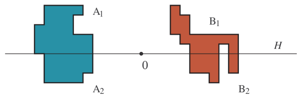
Figure 6.1. Two brick regions  A  and  B  divided by a line $H$ with the same area ratios.

Observe that the combined number of bricks in  $(\textnormal{A}_{1},\textnormal{B}_{1})$  is smaller than $k$, so inductive assumption applies. The same holds for  $(\textnormal{A}_{2},\textnormal{B}_{2})$. We then have:

$${\text{\rm area}}(\textnormal{A}+\textnormal{B})\ \geq\ {\text{\rm area}}(\textnormal{A}_{1}+\textnormal{B}_{1})\hskip 1.70709pt+\hskip 1.70709pt{\text{\rm area}}(\textnormal{A}_{2}+\textnormal{B}_{2})$$

$$\qquad\geq\ \left[\sqrt{{\text{\rm area}}(\textnormal{A}_{1})}\hskip 1.70709pt+\hskip 1.70709pt\sqrt{{\text{\rm area}}(\textnormal{B}_{1})}\right]^{2}\,+\,\left[\sqrt{{\text{\rm area}}(\textnormal{A}_{2})}\hskip 1.70709pt+\hskip 1.70709pt\sqrt{{\text{\rm area}}(\textnormal{B}_{2})}\right]^{2}$$

$$\qquad\geq\ \left[\sqrt{\theta\hskip 0.85355pt{\text{\rm area}}(\textnormal{A})}\hskip 1.70709pt+\hskip 1.70709pt\sqrt{\theta\hskip 0.85355pt{\text{\rm area}}(\textnormal{B})}\right]^{2}\,+\,\left[\sqrt{(1-\theta)\hskip 0.85355pt{\text{\rm area}}(\textnormal{A})}\hskip 1.70709pt+\hskip 1.70709pt\sqrt{(1-\theta)\hskip 0.85355pt{\text{\rm area}}(\textnormal{B})}\right]^{2}$$

$$\qquad\geq\ \bigl{[}\theta\hskip 0.85355pt+\hskip 0.85355pt(1-\theta)\bigr{]}\hskip 1.70709pt\left[\sqrt{{\text{\rm area}}(\textnormal{A})}\hskip 1.70709pt+\hskip 1.70709pt\sqrt{{\text{\rm area}}(\textnormal{B})}\right]^{2}\ =\ \sqrt{{\text{\rm area}}(\textnormal{A})}\hskip 1.70709pt+\hskip 1.70709pt\sqrt{{\text{\rm area}}(\textnormal{B})}\,.$$

Here the first inequality follows since sets  $\textnormal{A}_{1}+\textnormal{B}_{1}$  and  $\textnormal{A}_{2}+\textnormal{B}_{2}$  lie on different sides of $H$. The second inequality follows from induction assumption. The remaining inequalities are trivial equalities. This completes the proof. ∎

Proof of Theorem 6.16.

Let  $\textnormal{A},\textnormal{B}\subset\mathbb{R}^{2}$ be two convex polygons and let  $\varepsilon>0$. Consider the scaled square grid  $\varepsilon\hskip 0.85355pt\mathbb{Z}^{2}$  and denote by  $\textnormal{A}_{\varepsilon},\textnormal{B}_{\varepsilon}$  the unions of  $\varepsilon\times\varepsilon$  squares completely inside  $\textnormal{A},\textnormal{B}$. Observe that  ${\text{\rm area}}(\textnormal{A}_{\varepsilon})\to{\text{\rm area}}(\textnormal{A})$,  ${\text{\rm area}}(\textnormal{B}_{\varepsilon})\to{\text{\rm area}}(\textnormal{B})$,  and  ${\text{\rm area}}(\textnormal{A}_{\varepsilon}+\textnormal{B}_{\varepsilon})\to{\text{\rm area}}(\textnormal{A}+\textnormal{B})$,  as  $\varepsilon\to 0$. The result now follows by applying Lemma 6.20 to brick regions  $(\textnormal{A}_{\varepsilon},\textnormal{B}_{\varepsilon})$  and taking the limit. ∎

7. Final remarks

7.1. Our sources

As we mentioned in the introduction, this paper is written with expository purposes. We present no new results except for the tangential Theorem 4.9 which can only be understood in the context of the proof of Theorem 4.8 in Section 4. While the majority of the presentation is new, some of it borrows more or less directly from other sources. Here is a quick reference guide.

Section 3 is almost directly lifted from [CP21]. Parts of it are strongly influenced by [BH20] and [SvH19], notably the proof of Lemma 3.5. Section 4 is adapted and substantially simplified from [CP21], so much that it appears unrecognizable. Note that we omit the equality conditions which can be similarly adapted.

Section 5 was originally intended to be included in [CP21], but was left out when that paper exploded in size. The aim of that section is to emphasize that the Lorentzian polynomial approach in [ALOV18, BH20] is a special case of ours. There are many indirect connections to all three papers, but the presentation here seems novel. Note that there are several equivalent definitions of Lorentzian polynomials (see [BH20, §2]), and we choose the one closest to our context for convenience.

Section 6 came largely as a byproduct of our original effort in [CP21] to understand Stanley’s inequality via the proof of the Alexandrov–Fenchel inequality in [SvH19] and Stanley’s original paper [Sta81]. In an effort to make the presentation self-contained, we borrow liberally from [Sch14]. Our presentation of the Brunn–Minkowski inequality is standard and follows [Mat02, $\S$12.2] and [Pak09, $\S$7.7, §41.4].

Note that in our presentation, the totality of the proof of the Alexandrov–Fenchel inequality is a rather lengthy union of Section 3 and Section 6. There are several other relatively recent proofs [CKMS19, KK12, SvH19, Wang18] based on different ideas and which employ existing technologies to a different degree. Obviously, the notions of “simple” and “self-contained” we used in the introductions are subjective, so we can only state our own view. Similarly, we challenge the assessment in [KK12] which call their proof “elementary”.

Let us single out [CKMS19] which relates the proof of the Alexandrov–Fenchel inequality in [SvH19] and (implicitly) the polynomial method in [BH20]. Although our work is independent of [CKMS19], it would be curious to see if that method can be extended to the full power of the combinatorial atlas technology in [CP21].

Finally, let us mention that in the special case of brick polytopes, our proof of the Alexandrov–Fenchel inequality simplifies so much that it becomes known and elegantly presented in [vL81]. See also [Gur08] for a generalization and a modern treatment from the Lorentzian polynomial point of view.

7.2. Stanley’s inequality

Recall the straightforward derivation of Stanley’s inequality (for the number of certain linear extensions in posets) from the Alexandrov–Fenchel inequality given in [Sta81]. Given the linear algebraic proof of the latter in Section 6, one can ask why do we have such a lengthy proof of them in [CP21, $\S$14]. There are two reasons for this, one technical and one structural.

The technical reason is that our approach allows us to obtain $q$-analogues and more general deformations of Stanley’s inequality, which do not seem to follow directly from the Alexandrov–Fenchel inequality. The structural reason is that we really aim to rederive the equality conditions for Stanley’s inequality which were recently obtained by a difficult argument in a breakthrough paper [SvH20+].

In a nutshell, we employ self-similarity inherent to the problem, in terms of faces of order polytopes used to translate the problem into geometry. Applying iteratively the argument in our proof of the Alexandrov–Fenchel inequality, allowed us to streamline the construction and make it completely explicit if rather lengthy. This, in turn, gave both the equality conditions and the deformations mentions above.

It would be interesting to see if the argument along these lines can be replicated in other cases. In particular, the Kahn–Saks inequality in [KS84] is the closest to Stanley’s inequality, and yet does not have a combinatorial atlas proof. Note that the equality conditions are also harder to obtain in this case, and they are not even conjectured at this point, see [CPP21, $\S$8.3].

Finally, let us emphasize that our proof of the Alexandrov–Fenchel inequality does not extend to give the equality conditions in full generality. There are two reasons for this: parallel translations of the facets and the need to take limits. While the former is “combinatorial” and is an obstacle to making the equality characterization explicit, the latter is more critical as taking limits can create equalities.

To appreciate the distinction, the reader can think of convex polygons in the plane, where the usual isoperimetric inequality is always strict vs. the circle which is the limit of such polygons, and where the isoperimetric inequality is an equality. While the equality conditions are classically understood for the Brunn–Minkowski inequality [BuZ88, $\S$8] and for the polytopal case of the Alexandrov–Fenchel inequality [SvH20+], for general convex bodies new ideas are needed.

7.3. Simplicial complexes

Theorem 4.7 shows that an abstract simplicial complex is necessarily a matroid if the corresponding combinatorial atlas satisfies (Hyp). In a way, this result is comparable to the equivalence between Lorentzian polynomials and $M$-convexity in [BH20, Thm 3.10 (1)–(7)].

In fact, there are many simplicial complexes for which the sequence  $({\textrm{I}}_{k})_{k\geq 0}$  of number of faces of cardinality $k$, is not unimodal, let alone log-concave. The face lattice of simplicial complexes is especially interesting and well studied. In this case, unimodality was known as the Motzkin conjecture (1961), which was disproved in [Bjö81]. There, Björner gave an example of a $24$-dimensional simplicial polytopes for which the  $f$-vector is not unimodal. See also smaller examples in [BL81, Bjö94] of $20$-dimensional simplicial polytopes, and [Eck06] which proved that this dimension cannot be lowered.

Finally, let us mention that in Section 4 we start with a simplicial complex and then we build an atlas, while in Section 5 we build an atlas starting with a Lorentzian polynomial. On the other hand, in [ALOV19], the authors start with a Lorentzian polynomial and then build a simplicial complex. The connection between these approaches is yet to be fully understood.

Acknowledgements

We are grateful to Matt Baker, June Huh, Jeff Kahn, Gaiane Panina, Greta Panova, Yair Shenfeld, Hunter Spink, Ramon van Handel and Cynthia Vinzant for helpful discussions and remarks on the subject. The first author was partially supported by the Simons Foundation. The second author was partially supported by the NSF.

References

• [AHK18] Karim Adiprasito, June Huh and Eric Katz, Hodge theory for combinatorial geometries, Annals of Math. 188 (2018), 381–452.
• [Ale50] Alexander D. Alexandrov, Convex polyhedra (translated from the 1950 Russian original), Springer, Berlin, 2005, 539 pp.
• [ALOV18] Nima Anari, Kuikui Liu, Shayan Oveis Gharan and Cynthia Vinzant, Log-concave polynomials III: Mason’s Ultra-log-concavity conjecture for independent sets of matroids, preprint (2018), 11 pp.;  arXiv:1811.01600.
• [ALOV19] Nima Anari, Kuikui Liu, Shayan Oveis Gharan and Cynthia Vinzant, Log-concave polynomials II: High-dimensional walks and an FPRAS for counting bases of a matroid, in Proc. 51-st STOC, ACM, New York, 2019, 1–12.
• [BL81] Louis J. Billera and Carl W. Lee, A proof of the sufficiency of McMullen’s conditions for $f$-vectors of simplicial convex polytopes, J. Combin. Theory, Ser. A 31 (1981), 237–255.
• [Bjö81] Anders Björner, The unimodality conjecture for convex polytopes, Bull. AMS 4 (1981), 187–188.
• [Bjö94] Anders Björner, Partial unimodality for $f$-vectors of simplicial polytopes and spheres, Contemp. Math. 178 (1994), 45–54.
• [BjZ92] Anders Björner and Günter M. Ziegler, Introduction to greedoids, in Matroid applications, Cambridge Univ. Press, Cambridge, UK, 1992, 284–357.
• [BH20] Petter Brändén and June Huh, Lorentzian polynomials, Annals of Math. 192 (2020), 821–891.
• [BuZ88] Yuri D. Burago and Victor A. Zalgaller, Geometric inequalities, Springer, Berlin, 1988, 331 pp.
• [CP21] Swee Hong Chan and Igor Pak, Log-concave poset inequalities, preprint (2021), 71 pp; arXiv: 2110.10740.
• [CPP21] Swee Hong Chan, Igor Pak and Greta Panova, Extensions of the Kahn–Saks inequality for posets of width two, preprint (2021), 25 pp.;  arXiv:2106.07133.
• [COSW04] Young-Bin Choe, James G. Oxley, Alan D. Sokal and David G. Wagner, Homogeneous multivariate polynomials with the half-plane property, Adv. Appl. Math. 32 (2004), 88–187.
• [CKMS19] Dario Cordero-Erausquin, Bo’az Klartag, Quentin Merigot and Filippo Santambrogio, One more proof of the Alexandrov–Fenchel inequality, C. R. Math. Acad. Sci. Paris 357 (2019), no. 8, 676–680.
• [Eck06] Jürgen Eckhoff, Combinatorial properties of $f$-vectors of convex polytopes, Normat 54 (2006), 146–159.
• [Gre81] Jiří Gregor, On quadratic Hurwitz forms, Apl. Mat. 26 (1981), 142–153.
• [Gur08] Leonid Gurvits, Van der Waerden/Schrijver-Valiant like conjectures and stable (aka hyperbolic) homogeneous polynomials: one theorem for all, Electron. J. Combin. 15 (2008), no. 1, RP 66, 26 pp.
• [HG20] Daniel Hug and Wolfgang Weil, Lectures on convex geometry, Springer, Cham, 2020, 287 pp.
• [HSW22] June Huh, Benjamin Schröter and Botong Wang, Correlation bounds for fields and matroids, Jour.  EMS 24 (2022), 1335–1351.
• [KS84] Jeff Kahn and Michael Saks, Balancing poset extensions, Order 1 (1984), 113–126.
• [KK12] Kiumars Kaveh and Askold Khovanskii, Algebraic equations and convex bodies, in Perspectives in analysis, geometry, and topology, Birkhäuser, New York, 2012, 263–282.
• [KLS91] Bernhard Korte, László Lovász and Rainer Schrader, Greedoids, Springer, Berlin, 1991, 211 pp.
• [Mas72] John H. Mason, Matroids: unimodal conjectures and Motzkin’s theorem, in Proc. Conf. Combin. Math., Inst. Math. Appl., Southend-on-Sea, UK, 1972, 207–220; available at  tinyurl.com/7w7wjz6v
• [Mat02] Jiří Matoušek, Lectures on Discrete Geometry, Springer, New York, 2002, 481 pp.
• [Pak09] Igor Pak, Lectures on discrete and polyhedral geometry, monograph draft (2009), 440 pp.; available at
math.ucla.edu/~pak/book.htm
• [Sch14] Rolf Schneider, Convex bodies: the Brunn–Minkowski theory (second ed.), Cambridge Univ. Press, Cambridge, UK, 2014, 736 pp.
• [SvH19] Yair Shenfeld and Ramon van Handel, Mixed volumes and the Bochner method, Proc. AMS 147 (2019), 5385–5402.
• [SvH20+] Yair Shenfeld and Ramon van Handel, The extremals of the Alexandrov–Fenchel inequality for convex polytopes, Acta Math., to appear, 82 pp.;  arXiv:2011.04059.
• [Sta81] Richard P. Stanley, Two combinatorial applications of the Aleksandrov–Fenchel inequalities, J. Combin. Theory, Ser. A 31 (1981), 56–65.
• [vL81] Jacobus H. van Lint, Notes on Egoritsjev’s proof of the van der Waerden conjecture, Linear Algebra Appl. 39 (1981), 1–8.
• [Wang18] Xu Wang, A remark on the Alexandrov–Fenchel inequality, J. Funct. Anal. 274 (2018), 2061–2088.