CAFE: Learning to Condense Dataset by Aligning Features

Abstract

Dataset condensation aims at reducing the network training effort through condensing a cumbersome training set into a compact synthetic one. State-of-the-art approaches largely rely on learning the synthetic data by matching the gradients between the real and synthetic data batches. Despite the intuitive motivation and promising results, such gradient-based methods, by nature, easily over-fit to a biased set of samples that produce dominant gradients, and thus lack a global supervision of data distribution. In this paper, we propose a novel scheme to Condense dataset by Aligning FEatures (CAFE), which explicitly attempts to preserve the real-feature distribution as well as the discriminant power of the resulting synthetic set, lending itself to strong generalization capability to various architectures. At the heart of our approach is an effective strategy to align features from the real and synthetic data across various scales, while accounting for the classification of real samples. Our scheme is further backed up by a novel dynamic bi-level optimization, which adaptively adjusts parameter updates to prevent over-/under-fitting. We validate the proposed CAFE across various datasets, and demonstrate that it generally outperforms the state of the art: on the SVHN dataset, for example, the performance gain is up to 11%. Extensive experiments and analysis verify the effectiveness and necessity of proposed designs.

1 Introduction

Deep neural networks (DNNs) have demonstrated unprecedented results in many if not all applications in computer vision [9, 21, 39, 27, 10, 23, 29, 8, 46, 49, 28, 38, 37, 36]. These gratifying results, nevertheless, come with costs: the training of DNNs heavily rely on the sheer amount of data, sometimes up to tens of millions of samples, which consequently requires enormous computational resources.

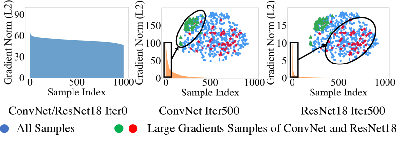
(a)

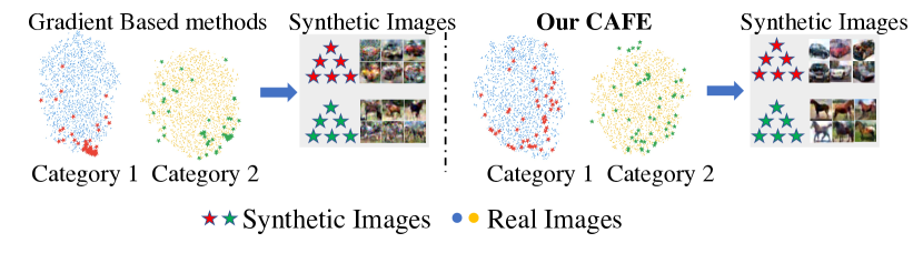
(b)

Figure 1: (a) At the later training stage, most examples do not contribute meaningful gradients, making the synthetic set learned by gradient matching extremely bias towards those large-gradient samples, which downgrades its generalization to unseen architectures. (b) Compared with gradient-based method [53], the synthetic set learned by our approach effectively captures the whole distribution thus generalizes well to other network architectures.

Numerous research endeavours have, therefore, focused on alleviating the cumbersome training process through constructing small training sets [1, 14, 7, 13, 42, 31, 33, 44, 45, 50]. One classic approach is known as coreset or subset selection [1, 31, 12], which aims to obtain a subset of salient data points to represent the original dataset of interest. Nevertheless, coreset selection is typically a NP-hard problem [19], making it computationally intractable over large-scale datasets. Most existing approaches have thus resorted to greedy algorithms with heuristics [7, 31, 2, 47, 35] to speed up the process by trading-off the optimality.

Recently, dataset condensation [40, 53, 6] has emerged as a competent alternative with promising results. The goal of dataset condensation is, as its name indicates, to condense a large training set into a small synthetic one, upon which DNNs are trained and expected to preserve the performances. Along this line, the pioneering approach of [40] proposed a meta-learning-based strategy; however, the nest-loop optimization precludes its scaling up to large-scale in-the-wild datasets. The work of [53] alleviates this issue by enforcing the batch gradients of the synthetic samples to approach those of the original ones, which bypasses the recursive computations and achieves impressive results. The optimization of the synthetic examples is explicitly supervised by minimizing the distance between the gradients produced by the synthetic dataset and the real dataset.

However, gradient matching method has two potential problems. First, due to the memorization effect of deep neural networks [48], only a small number of hard examples or noises produce dominant gradients over the network parameters. Thus, gradient matching may overlook those representative but easy samples, while overfit to those hard samples or noises. Second, these hard examples that produce large gradients may vary across different architectures; relying solely on gradients, therefore, will yield poor generalization performance to unseen architectures. The distributions of gradients and hard examples are illustrated in Fig. 1(a). The synthetic data learned by gradient matching may be highly biased towards a small number of unrepresentative data points, which is illustrated in Fig. 1(b).

To go beyond the learning bias and better capture the whole dataset distribution, in this paper, we propose a novel strategy to Condense dataset by Aligning FEatures, termed as CAFE. Unlike the approach of [53], we account for the distribution consistency between synthetic and real datasets by applying distribution-level supervision. Our approach, through matching the features that involve all intermediary layers, expands the attention across all samples and hence provides a much more comprehensive characterization of the distribution while avoiding over-fitting on hard or noisy samples. Such distribution-level supervision will, in turn, endow CAFE with stronger generalization power than gradient-based methods, since the hard examples may easily vary across different architectures.

Specifically, we impose two complementary losses into the objective of CAFE. The first one concerns capturing the data distribution, in which the layer-wise alignment between the features of the real and synthetic samples is enforced and further the distribution is preserved. The second loss, on the other hand, concerns discrimination. Intuitively, the learned synthetic samples from one class should well represent the corresponding clusters of the real samples. Hence, we may treat each real sample as a testing sample, and classify it based on its affinity to the synthetic clusters. Our second loss is then defined upon the classification result of the real samples, which, effectively, injects the discriminant capabilities into the synthetic samples.

The proposed CAFE is further backed up by a novel bi-level optimization scheme, which allows our network and synthetic data to be updated through a customized number of SGD steps. Such a dynamic optimization strategy, in practice, largely alleviates the under- and over-fitting issues of prior methods. We conduct experiments on several popular benchmarks and demonstrate that, the results yielded by CAFE are significantly superior to the state of the art: on the SVHN dataset, for example, our method outperforms the runner-up by $11\%$ when learning 1 image/class synthetic set. We also especially prove that synthetic set learned by our method has better generalization ability than that learned by [53].

In summary, our contribution is a novel and effective approach for condensing datasets, achieved through aligning layer-wise features between the real and synthetic data, and meanwhile explicitly encoding the discriminant power into the synthetic clusters. In addition, a new bi-level optimization scheme is introduced, so as to adaptively alter the number of SGD steps. These strategies jointly enable the proposed CAFE to well characterize the distribution of the original samples, yielding state-of-the-art performances with strong generalization and robustness across various learning settings.

2 Related Work

Dataset Condensation.

Several methods have been proposed to improve the performance, scalability and efficiency of dataset condensation. Based on the meta-learning method proposed in [40], some works [4, 25, 26] try to simplify the inner-loop optimization of a classification model by training with ridge regression which has a closed-form solution. [34] trains a generative network to produce the synthetic set. The generative network is trained using the same objective as [40]. To improve the data efficiency of [53], differentiable Siamese augmentation is proposed in [51]. They enable the synthetic data to train neural networks with data augmentation effectively.

A recent work [52] also learns synthetic set with feature distribution matching. Our method is different from it in three main aspects: 1) we match layer-wise features while [52] only uses final-layer features; 2) we further explicitly enable the synthetic images to be discriminative as the classifier (Sec. 3.3); 3) our method includes a dynamic bi-level optimization which can boost the performance with adaptive SGD steps, while [52] tries to reduce the training cost by dropping the bi-level optimization.

Coreset Selection.

The classic technique to condense the training set size is coreset or subset selection [1, 7, 15, 41]. Most of these methods incrementally select important data points based on heuristic selection criteria. For example, [31] selects data points that can approach the cluster centers. [2] tries to maximize the diversity of samples in the gradient space. [35] measures the forgetfulness of trained samples during network training and drops those that are not easy to forget. However, these heuristic selection criteria cannot ensure that the selected subset is optimal for training models, especially for deep neural networks. In addition, greedy sample selection algorithms are unable to guarantee that the selected subset is optimal to satisfy the criterion.

Generative Models

Our work is also closely related to generative model such as auto-encoder [18] and generative adversarial networks (GANs) [16, 24]. The difference is that image generation aims to synthesize real-looking images that can fool human beings, while our goal is to generate informative training samples that can be used to train deep neural networks more efficiently. As shown in [53], concerning training models, the efficiency of these images generated by GANs closes to that of randomly sampled real images. In contrast, our method can synthesize better training images that significantly outperform those selected real images in terms of model training.

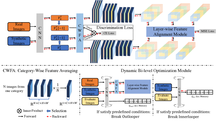
Figure 2: Illustration of the proposed CAFE method. The CAFE consists of a layer-wise feature alignment module to capture the accurate distribution of the original large-scale dataset, a discrimination loss for mining the discriminate samples from real dataset, and a dynamic bi-level optimization module to reduce the influence of under- and over-fitting on synthetic images.

3 Method

In this section, we first briefly overview the proposed CAFE. Then, we introduce three carefully designed modules: layer-wise feature alignment module, discrimination loss, and dynamic bi-level optimization module.

3.1 Overview

Dataset condensation aims to condense a large-scale dataset $\mathcal{T}=\{(\bm{x}_{i},y_{i})\}|^{|\mathcal{T}|}_{i=1}$ into small (synthetic) dataset $\mathcal{S}=\{(\bm{s}_{j},y_{j})\}|^{|\mathcal{S}|}_{j=1}$ while achieving similar generalization performance. Fig. 2 illustrates the proposed method. First, we sample two data batches from the large-scale dataset $\mathcal{T}$ and the learnable synthetic set $\mathcal{S}$ respectively, and then extract the features using neural network $\phi_{\bm{\theta}}(\cdot)$ which is parameterized with $\bm{\theta}$. To capture the distribution of $\mathcal{T}$ accurately, layer-wise feature alignment module is designed, in which we minimize the difference of layer-wise feature maps of real and synthetic images using Mean Square Error (MSE). To enable learning discriminative synthetic images, we use the feature centers of synthetic images of each class to classify the real images by computing their inner-product and cross-entropy loss. The synthetic images are updated by minimizing the above two losses, which is the outer-loop. Then, we update the network $\phi_{\bm{\theta}}(\cdot)$ by minimizing the cross-entropy loss on synthetic images, which is the inner-loop. The synthetic images and network are alternatively using a novel dynamic bi-level optimization algorithm which avoids the over- or under-fitting on synthetic dataset and breaks the outer- and inner-loop automatically.

3.2 Layer-wise Features Alignment

As mentioned above, previous works [53, 51] compare the differences of gradients between real and synthetic data. Such objective produces samples with large gradients, but these samples fail to capture the distribution of the original dataset (illustrated in Fig. 5). Thus, it may have poor performance when generalizing to unseen architectures. To tackle this issue, we design Category-Wise Feature Averaging (CWFA), illustrated in Fig. 2, to measure the feature difference between $\mathcal{T}$ and $\mathcal{S}$ at each convolutional layer. Specifically, we sample a batch of real data $\mathcal{T}_{k}$ and synthetic data $\mathcal{S}_{k}$ with the same label $k$ and the batch size $N$ and $M$, from $\mathcal{T}$ and $\mathcal{S}$ respectively. We embed each real and synthetic datum using network $\phi_{\bm{\theta}}(\cdot)$ with $L$ layers (except the output layer) and obtain the layer-wise features $\bm{F}^{\mathcal{T}}_{k}=[\bm{f}^{\mathcal{T}}_{k,1},\bm{f}^{\mathcal{T}}_{k,2},...,\bm{f}^{\mathcal{T}}_{k,L}]=\phi_{\bm{\theta}}(\mathcal{T}_{k})$ and $\bm{F}^{\mathcal{S}}_{k}=[\bm{f}^{\mathcal{S}}_{k,1},\bm{f}^{\mathcal{S}}_{k,2},...,\bm{f}^{\mathcal{S}}_{k,L}]=\phi_{\bm{\theta}}(\mathcal{S}_{k})$. The $l^{\text{th}}$ layer feature $\bm{f}^{\mathcal{T}}_{k,l}\in\mathbb{R}^{N\times C^{\prime}}$ is reduced to ${\bar{\bm{f}}^{\mathcal{T}}_{k,l}}\in\mathbb{R}^{1\times C^{\prime}}$ by averaging the $N$ samples in the real data batch, where $C^{\prime}=C\times H\times W$ and it refers to the feature size of corresponding layer. Similarly, we obtain ${\bar{\bm{f}}^{\mathcal{S}}_{k,l}}$ for synthetic data batch.

Then, MSE is applied to calculate the feature distribution matching loss $\mathcal{L}_{\text{f}}$ for every layer, which is formulated as

$$\mathcal{L}_{\text{f}}=\sum_{k=1}^{K}\sum_{l=1}^{L}|{\bar{\bm{f}}^{\mathcal{S}}_{k,l}}-{\bar{\bm{f}}^{\mathcal{T}}_{k,l}}|^{2},$$ (1)

where $K$ is the number of categories in a dataset.

3.3 Discrimination Loss

Though the layer-wise feature alignment can capture the distribution of original dataset, it may overlook the discriminative sample mining. We hold the view that an informative synthetic set could be used as a classifier to classify real samples. Based on this, we calculate the classification loss in the last-layer feature space. we obtain the synthetic feature center $\bar{\bm{f}}^{\mathcal{S}}_{k,L}\in\mathbb{R}^{1\times C^{\prime}}$ of each category $k$ by averaging the batch. We concatenate the feature centers $\bar{\bm{F}}^{\mathcal{S}}_{L}=[\bar{\bm{f}}^{\mathcal{S}}_{1,L},\bar{\bm{f}}^{\mathcal{S}}_{2,L},...,\bar{\bm{f}}^{\mathcal{S}}_{K,L}]$ and also real data $\bm{F}^{\mathcal{T}}_{L}=[\bm{f}^{\mathcal{T}}_{1,L},\bm{f}^{\mathcal{T}}_{2,L},...,\bm{f}^{\mathcal{T}}_{K,L}]$ from all classes. The real data is classified using the inner-product between real data and the synthetic centers

$$\mathbf{O}=\left<\bm{F}^{\mathcal{T}}_{L},{(\bar{\bm{F}}^{\mathcal{S}}_{L})}^{\text{T}}\right>,$$ (2)

where $\mathbf{O}\in\mathbb{R}^{N^{\prime}\times K}$ contains the logists of $N^{\prime}=K\times N$ real data points. The classification loss is

$$\mathcal{L}_{\text{d}}=-\frac{1}{N^{\prime}}\Sigma_{i=1}^{N^{\prime}}\log p_{i},$$ (3)

where the probability $p_{i}$ is the softmax value corresponding to its ground-truth label over all classes $p_{i}=\text{softmax}(\mathbf{O}_{i})$. The total loss for learning synthetic images is

$$\mathcal{L}_{\text{total}}=\mathcal{L}_{\text{f}}+\beta\mathcal{L}_{\text{d}},$$ (4)

where $\beta$ is a positive scalar weight of $\mathcal{L}_{\text{d}}$. We study the influence of $\beta$ in Sec. 4.3. The synthetic set is updated by minimizing $\mathcal{L}_{\text{total}}$:

$$\mathcal{S}\leftarrow\operatorname*{arg\,min}_{\mathcal{S}}\mathcal{L}_{\text{total}}$$ (5)

Algorithm 1 Dynamic Bi-level Optimization

$\mathcal{T}$ and $\mathcal{S}$ are the real the synthetic datasets. $\epsilon$ is a random sampling function for selecting $N$ images from $K$ categories. $Q_{out}$ and $Q_{in}$ are the queues to save the performance on real dataset in outer- and inner-loop, respectively. div($\cdot$) is a function that calculates the difference between maximum and minimum values of $Q_{out}$ and $Q_{in}$. $\gamma$ is the maximum length of queues. The default loop numbers of DC are $l_{out}$ and $l_{in}$. $l_{c}^{\cdot}$ represents the loop number of CAFE.

1:  while not converged do

2:     randomly initialize $\bm{\theta}$, $Q_{out}$ = []; $Q_{in}$ = []; $l_{c}^{out}$=$l_{c}^{in}$ = 0.

3:     while True do

4:        updating $\mathcal{S}$ using Eq. 5; $l_{c}^{out}$ += 1. {outer-loop}

5:        acc. = get$\_$acc$(\epsilon(K,N))$; $Q_{out}$.append(acc.).

6:        if  $|Q_{out}|$ == $\gamma$ and div($Q_{out}$)$<\lambda_{1}$ or $l_{c}^{out}>l_{out}$   then

7:           $l_{c}^{out}$ = 0, $Q_{out}$ = [].

8:           Break

9:        else

10:           $Q_{out}$.pop[0].

11:        end if

12:        while True do

13:           updating $\bm{\theta}$ using Eq. 6. {inner-loop}

14:           acc. = get$\_$acc$(\epsilon(K,N))$; $Q_{in}$.append(acc.)

15:           if  $|Q_{in}|$ == $\gamma$ and div($Q_{in}$)$>\lambda_{2}$ or $l_{c}^{in}>l_{in}$   then

16:              $l_{c}^{in}$ = 0, $Q_{in}$ = [].

17:              Break

18:           else

19:              $Q_{in}$.pop[0].

20:           end if

21:        end while

22:     end while

23:  end while

3.4 Dynamic Bi-level Optimization

Similar to previous work [40, 53], we also learn the synthetic set with a bi-level optimization, in which the synthetic set $\mathcal{S}$ is updated using Eq. 5 in the outer-loop and network parameters $\bm{\theta}$ is updated using

$$\bm{\theta}\leftarrow\operatorname*{arg\,min}_{\bm{\theta}}J(\mathcal{S},\bm{\theta})$$ (6)

in the inner-loop alternatively. $J(\mathcal{S},\bm{\theta})$ calculates the cross-entropy classification loss on the synthetic set $\mathcal{S}$. In this way, the synthetic set can be trained on many different $\bm{\theta}$ so that it can generalize to them. We initialize $\mathcal{S}$ and $\bm{\theta}$ from random noise and standard network random initialization [17]. Previous work [53, 51] sets a fixed number of outer-loop and inner-loop optimization steps, which takes too much time to adjust the hyper-parameters and may lead to networks’ over- or under-fitting on synthetic set. To address these issues, we design a new bi-level optimization algorithm that can break the outer- and inner-loop automatically. Fig. 2 illustrates the proposed dynamic bi-level optimization module. To monitor the changing of network parameters $\bm{\theta}$, we randomly sample some images from real training set as a query set to evaluate the network. Then, a queue $Q$ is used to store the performance on the query set. We expect to learn synthetic data on more diverse network parameters. Hence, we sample inner-loop networks to optimize synthetic images when remarkable performance improvement is achieved on the query set. The optimization will be stopped when the performance on the query set is converged. $\lambda_{1}$ and $\lambda_{2}$ are two hyper parameters of dynamic bi-level optimization. We implement ablation study to show that the performance is not sensitive to $\lambda_{1}$ and $\lambda_{2}$. The training algorithm is summarized in Alg. 1.

Table 1: The performance (testing accuracy %) comparison to state-of-the-art methods. LD^† and DD^† use LeNet for MNIST and AlexNet for CIFAR10, while the rest use ConvNet for training and testing. IPC: Images Per Class, Ratio (%): the ratio of condensed images to whole training set.

	IPC	Ratio %	Coreset Selection				Condensation						Whole Dataset
			Random	Herding	K-Center	Forgetting	DD†	LD†	DC	DSA	CAFE	CAFE+DSA
MNIST	1	0.017	64.9$\pm$3.5	89.2$\pm$1.6	89.3$\pm$1.5	35.5$\pm$5.6	-	60.9$\pm$3.2	91.7$\pm$0.5	88.7$\pm$0.6	93.1$\pm$0.3	90.8$\pm$0.5	99.6$\pm$0.0
	10	0.17	95.1$\pm$0.9	93.7$\pm$0.3	84.4$\pm$1.7	68.1$\pm$3.3	79.5$\pm$8.1	87.3$\pm$0.7	97.4$\pm$0.2	97.8$\pm$0.1	97.2$\pm$0.2	97.5$\pm$0.1
	50	0.83	97.9$\pm$0.2	94.8$\pm$0.2	97.4$\pm$0.3	88.2$\pm$1.2	-	93.3$\pm$0.3	98.8$\pm$0.2	99.2$\pm$0.1	98.6$\pm 0.2$	98.9$\pm 0.2$
FashionMNIST	1	0.017	51.4$\pm$3.8	67.0$\pm$1.9	66.9$\pm$1.8	42.0$\pm$5.5	-	-	70.5$\pm$0.6	70.6$\pm$0.6	77.1$\pm$0.9	73.7$\pm$0.7	93.5$\pm$0.1
	10	0.17	73.8$\pm$0.7	71.1$\pm$0.7	54.7$\pm$1.5	53.9$\pm$2.0	-	-	82.3$\pm$0.4	84.6$\pm$0.3	83.0$\pm$0.4	83.0$\pm$0.3
	50	0.83	82.5$\pm$0.7	71.9$\pm$0.8	68.3$\pm$0.8	55.0$\pm$1.1	-	-	83.6$\pm$0.4	88.7$\pm$0.2	84.8$\pm$0.4	88.2$\pm$0.3
SVHN	1	0.014	14.6$\pm$1.6	20.9$\pm$1.3	21.0$\pm$1.5	12.1$\pm$1.7	-	-	31.2$\pm$1.4	27.5$\pm$1.4	42.6$\pm$3.3	42.9$\pm$3.0	95.4$\pm$0.1
	10	0.14	35.1$\pm$4.1	50.5$\pm$3.3	14.0$\pm$1.3	16.8$\pm$1.2	-	-	76.1$\pm$0.6	79.2$\pm$0.5	75.9$\pm$0.6	77.9$\pm$0.6
	50	0.7	70.9$\pm$0.9	72.6$\pm$0.8	20.1$\pm$1.4	27.2$\pm$1.5	-	-	82.3$\pm$0.3	84.4$\pm$0.4	81.3$\pm$0.3	82.3$\pm$0.4
CIFAR10	1	0.02	14.4$\pm$2.0	21.5$\pm$1.2	21.5$\pm$1.3	13.5$\pm$1.2	-	25.7$\pm$0.7	28.3$\pm$0.5	28.8$\pm$0.7	30.3$\pm$1.1	31.6$\pm$0.8	84.8$\pm$0.1
	10	0.2	26.0$\pm$1.2	31.6$\pm$0.7	14.7$\pm$0.9	23.3$\pm$1.0	36.8$\pm$1.2	38.3$\pm$0.4	44.9$\pm$0.5	52.1$\pm$0.5	46.3$\pm$0.6	50.9$\pm$0.5
	50	1	43.4$\pm$1.0	40.4$\pm$0.6	27.0$\pm$1.4	23.3$\pm$1.1	-	42.5$\pm$0.4	53.9$\pm$0.5	60.6$\pm$0.5	55.5$\pm$0.6	62.3$\pm$0.4
CIFAR100	1	0.2	4.2$\pm$0.3	8.4$\pm$0.3	8.3$\pm$0.3	4.5$\pm$0.3	-	11.5$\pm$0.4	12.8$\pm$0.3	13.9$\pm$0.3	12.9$\pm$0.3	14.0$\pm$0.3	56.17$\pm$0.3
	10	2	14.6$\pm$0.5	17.3$\pm$0.3	7.1$\pm$0.2	9.8$\pm$0.2	-	-	25.2$\pm$0.3	32.3$\pm$0.3	27.8$\pm$0.3	31.5$\pm$0.2
	50	10	30.0$\pm$0.4	33.7$\pm$0.5	30.5$\pm$0.3	-	-	-	-	42.8$\pm$0.4	37.9$\pm$0.3	42.9$\pm$0.2

4 Experiments

In this section, we first introduce the used datasets and implementation details. Then, we compare the proposed method to the state-of-the-art methods. After that, we conduct sufficient ablation studies to analyze the significant components and the influence of hyper parameters. Finally, the visualizations of synthetic images and feature distributions are provided to show the superiority of our CAFE.

4.1 Datasets & Implementation Details

MNIST [22]. The MNIST is a handwritten digits dataset that is commonly used for validating image recognition models. It contains 60,000 training images and 10,000 testing images with the size of 28$\times$28.

FashionMNIST [43]. FashionMNIST is a dataset of Zalando’s article images, consisting of a training set of 60,000 examples and a test set of 10,000 examples. Each example is a 28$\times$28 gray-scale image, associated with a label from 10 classes.

SVHN [32]. SVHN is a real-world image dataset for developing machine learning and object recognition algorithms. It consists of over 600,000 digit images coming from real world data. The images are cropped to 32$\times$32.

CIFAR10/100 [20]. The two CIFAR datasets consist of tiny colored natural images with the size of 32$\times$32 from 10 and 100 categories, respectively. In each dataset, 50,000 images are used for training and 10,000 images for testing.

Implementation Details.

We present the experiments details of the outer-loop and inner-loop, respectively. In outer-loop, we optimize 1/10/50 Images Per Class (IPC) synthetic sets for all the five datasets using three-layer Convolutional Network (ConvNet) as same as [53]. The ConvNet includes three repeated “Conv-InstNorm-ReLU-AvgPool” blocks. The channel number of each convolutional layer is 128. The initial learning rate of synthetic images is 0.1, which is divided by 2 in 1,200, 1,400, and 1,800 iterations. We stop training in 2,000 iterations. For inner-loop, we train the ConvNet on synthetic sets for 300 epochs and evaluate the performances on 20 randomly initialized networks. The initial learning rate of network is 0.01. Following [53], we perform 5 experiments and report the mean and standard deviation on 100 networks. The default $N$ is 256, $\lambda_{1}$ is 0.05 and $\lambda_{2}$ is 0.05. We assess the sensitiveness of $\lambda_{1}$ and $\lambda_{2}$ in the Sec. 4.3.

4.2 Comparison to the State-of-the-art Methods

We compare our method to four coreset selection methods, namely Random [7, 30], Herding [5, 3], K-Center [11, 31] and Forgetting [35]. We also make comparisons to recent state-of-the-art condensation methods, namely Dataset Distillation (DD) [40], LD [4], Dataset Condensation (DC) [53] and DSA (adding differentiable Siamese augmentation for DC) [51]. Although state-of-the-art performances are achieved in [25, 26], we do not compare to them due to the remarkable difference in training scheme and cost. We report the performances of our method and competitors on five datasets in Tab. 1. When learning 1 image per class, our method achieves the best results on all the 5 datasets. In particular, the improvements on SVHN and FashionMNIST are 11% and 6.5% over other methods. Condensation-based methods outperforms than coreset selection methods with a large margin. Among coreset selection methods, Herding and K-Center outperform Random and Forgetting with a large margin. When learning 10 and 50 images/class, the performance of our method exceeds DC with 0.7%$\sim$2.6% on most datasets. Compared with DSA, Our CAFE+DSA achieves comparable results with DSA on most datasets on CIFAR10/100. For 50 images/class learning on CIFAR10, our CAFE+DSA outperforms DSA by 1.7%.

Table 2: Evaluation of the three components in CAFE

DL	LFA	Dynamic Bi-level Opt.	Performance
✓			49.78
	✓		53.96
✓	✓		54.53
✓		✓	50.92
	✓	✓	54.98
✓	✓	✓	55.50

4.3 Ablation Studies

In this subsection, we study ablations using CIFAR10 (IPC = 50) to investigate the effectiveness of each module and the influence of the hyper parameters.

Evaluation of the three components in CAFE.

To explore the effect of each component in our method, we design ablation studies of Discrimination Loss (DL), Layer-wise Feature Alignment (LFA) and Dynamic Bi-level Optimization on CIFAR10. As shown in Tab. 2, DL, LFA and Dynamic Bi-level Opt. are complementary with each other. CAFE performs poorly when using DL individually (49.78%), as DL focuses more on classifying the real samples but ignores the distribution consistency with real images. The result of using LFA individually outperforms DL with 4.18%, which implies considering of distribution consistency is more important for dataset condensation. However, utilizing LFA independently means the importance of all the images in real dataset are equal, which may overlook the information from discriminative samples (i.e. samples nearby the decision boundaries). Jointly using DL and LFA can obtain better result than using DC on CIFAR10 testing set. Adding the Dynamic Bi-level Opt. can further improve the performance of DL and LFA, which indicates breaking out-/inner-looper automatically can reduce the over-/under-fitting effectively. Using these three components together achieves the highest result. To understand the effect of DL and LFA more intuitively, we also visualize the synthetic images feature distributions of using DL or LFA independently in Sec. 4.4.

Table 3: Evaluation of the importance of layer-wise feature alignment. The layer1 is closest to the output layer while layer4 is closest to input layer. Note that, layer4 represents the last average pooling layer in ConvNet.

Layer1	Layer2	Layer3.	Layer4	Performance/+DL
✓				50.74/52.78
	✓			43.45/49.30
		✓		44.52/49.08
			✓	51.30/52.05

Exploring the importance of layer-wise feature alignment in each layer.

To investigate the importance of feature alignment, we apply the feature alignment operation to each layer individually. As shown in Tab. 3, the performances of different layers vary remarkably. Applying feature alignment operation in layer1 or layer4 obtains better results than in layer2 or layer3, as the supervision in layer2 or layer3 is far from the input and output layers. Applying feature alignment in each layer individually can not obtain promising results. To demonstrate the effectiveness of DL in each layer, we also show the results of adding DL loss. The addition of DL can consistently improve the performances in all layers.

Table 4: Evaluation of complementarity of layer-wise feature alignment. The indexes of layers are same as Tab. 3.

Layer1	Layer2	Layer3.	Layer4	Performance/+DL
✓				50.74/52.78
✓	✓			51.27/53.28
✓	✓	✓		53.16/53.96
✓	✓	✓	✓	54.98/55.50

(a) Ablation of $\lambda_{1}$.

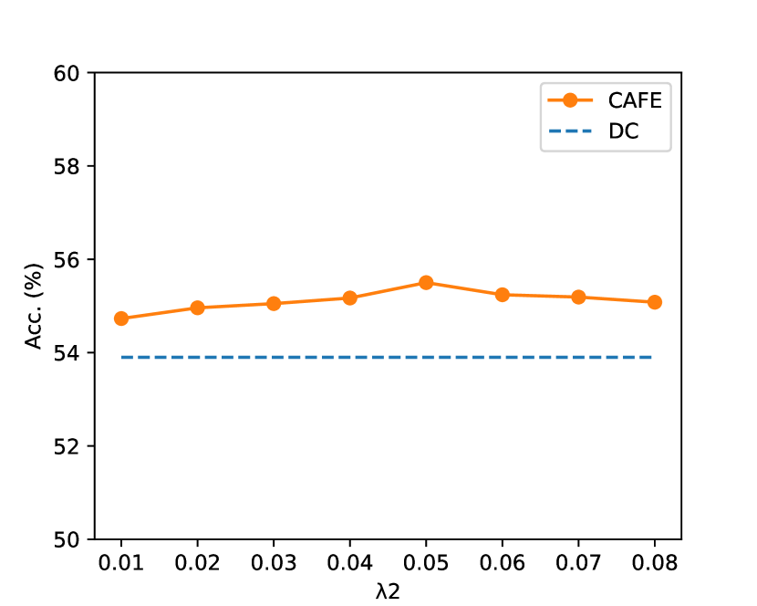
(b) Ablation of $\lambda_{2}$.

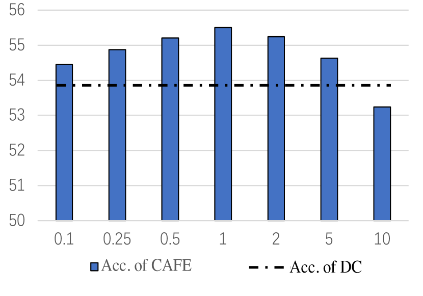
(c) Ablation of $\beta$.

Figure 3: $\lambda_{1}$ and $\lambda_{2}$ are the hyper-parameters in dynamic bi-level optimization module. $\beta$ is the ratio between $\mathcal{L}_{\text{f}}$ and $\mathcal{L}_{\text{d}}$.

Exploring the complementarity of layer-wise feature alignment among all layers.

After evaluating the importance of the LFA in each layer, exploring the complementarity of LFA in all layers is also very important. We first utilize the feature alignment in the layer1 to update the synthetic images. Then, we apply the same feature alignment to other layers (i.e. layer2, layer3, layer4). Here, we also consider the effect of DL and report the results with and without using DL in Tab. 4. When adding feature alignment to more layers, the performances on testing set become better. Meanwhile, the DL can further improve the performance in all cases. Specifically, the performance difference between using LFA in all layers and using in the first layer is about 4% (w/o DL) and 3% (with DL). The average performance boost of adding each layer is about 1% (w/o DL) and 0.7% (with DL), which indicates the strong complementarity of layer-wise feature alignment in all layers.

Table 5: Evaluation of $\gamma$ and the training time.

$\gamma$	5	10	15	20	DC
Accuracy (%)	53.16	55.50	54.10	53.63	53.9
Time (minutes)	$\approx$117	$\approx$367	$\approx$463	$\approx$463	$\approx$460

Evaluation of $\lambda_{1}$ and $\lambda_{2}$.

$\lambda_{1}$ and $\lambda_{2}$ are the thresholds to control whether break the out-looper and inner-looper or not. As shown in Fig. 3(a) and 3(b), we study different values of $\lambda_{1}$ and $\lambda_{2}$ ranging from 0.01 to 0.08. Our default $\lambda_{1}$ = 0.05 and $\lambda_{2}$ = 0.05 achieve the best results, which outperforms DC 1.6%. For out-looper, too large $\lambda_{1}$ may reduce the iterations of updating the synthetic images, which leads to the worse results. Too small $\lambda_{1}$ increases the optimization difficulties and even makes the model unable to break the out-looper normally. As for inner-looper, the model diversity is not large enough when $\lambda_{2}$ is too small, whereas it would be tricky to break the inner-looper when $\lambda_{2}$ is very large. Furthermore, it is worth noting that our method outperforms DC with a large margin at almost all settings. Meanwhile, the performance is not sensitive to $\lambda_{1}$ and $\lambda_{2}$.

Evaluation of the ratio $\beta$.

In Fig. 3(c), we evaluate the effect of different ratios between the $\mathcal{L}_{\text{f}}$ and $\mathcal{L}_{\text{d}}$. We find that setting equal weight for each loss achieves the best results. The performance gets promoted as $\beta$ increase from 0.1 to 1, while increasing the weight of $\mathcal{L}_{\text{d}}$ from 1 to 10 dramatically degrades performance.

Evaluation of $\gamma$ and the training time.

$\gamma$ is hyper parameter of the maximum length of queues in dynamic bi-level optimization. We show the performances and training time of different $\gamma$ in Tab. 5. One can find the default $\gamma=10$ achieves the best result and requires less time than DC. Too small and too large $\gamma$ may lead to under- or over-fitting.

Evaluation of the generalization to unseen architectures

To evaluate the generalization ability of synthetic data on unseen architectures, we first condense CIFAR10 dataset with ConvNet to generate synthetic images. Then, we train different architectures, including AlexNet, VGG11, ResNet18, and MLP (3 layers), on the synthetic images. As shown in Tab. 6, our method achieves better generalization performance than DC obviously. Specifically, our method outperforms DC with 5.25%, 1.79%, 4.42%, and 7.96% when testing on AlexNet, VGG11, ResNet18, and MLP (3 layers).

Table 6: The testing performance (%) on unseen architectures. The 50 IPC synthetic set is learned on one architecture (C), and then tested on another architecture (T).

	C\T	ConvNet	AlexNet	VGG11	ResNet18	MLP
DC	ConvNet	53.9$\pm$0.5	28.77$\pm$0.7	38.76$\pm$1.1	20.85$\pm$1.0	28.71$\pm$0.7
CAFE	ConvNet	55.50$\pm$0.4	34.02$\pm$0.6	40.55$\pm$0.8	25.27$\pm$0.9	36.67$\pm$0.6

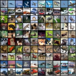
(a)

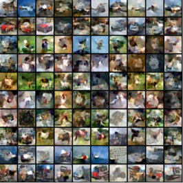
(b)

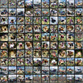
(c)

Figure 4: Visualizations of original images, and synthetic images generated by CAFE and DC. Both CAFE and DC are initialized from random noise.

4.4 Visualizations

In this subsection, we visualize the synthetic images as well as data distribution to show the effectiveness of CAFE.

Synthetic images.

To make fair comparison, the synthetic set is initialized by the same random noise (IPC = 50). After that, we apply DC and CAFE to optimize the synthetic set on CIFAR10 dataset. Finally, the partial (only show 10 images per class) optimized synthetic images and original images of CIFAR10 are shown in Fig. 4. There are several observations can be summarized as follows: 1). It is easy to find that the synthetic images generated by our method is more visually similar to original CIFAR10 images than DC. 2). The synthetic images have more semantic information than DC, which illustrates the effectiveness of LFA and DL modules. 3). A certain ratio of images generated by DC are not very clear, which could not provide enough discriminative features for classification.

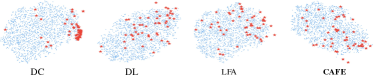
Figure 5: The data distribution of real images and synthetic images learned by DC [53], DL, LFA, and CAFE for one category in CIFAR10.

Data distribution.

To evaluate whether the synthetic images using our method can capture more accurate distribution from original dataset, we utilize t-SNE to visualize the features of real set and synthetic sets generated by DC, DL, LFA and CAFE. As shown in Fig. 5, the “points” and “stars” represent the real and synthetic features. The synthetic images of DC gather around a small area of decision boundary, which indicates using DC can not capture the original distribution well. Our methods DL, LFA, and CAFE effectively capture useful information across the whole real dataset, which possesses a good generalization among different CNN architectures.

5 Conclusion

In this work, we propose a novel scheme to Condense dataset by Aligning FEatures (CAFE), which explicitly attempts to preserve the real-feature distribution as well as the discriminant power of the resulting synthetic data, lending itself to strong generalization capability to unseen architectures. The CAFE consists of three carefully designed modules, namely layer-wise feature alignment module, discrimination loss, and dynamic bi-level optimization module. The feature alignment module and discrimination loss concern capturing distribution consistency between synthetic and real sets, while bi-level optimization enables CAFE to learn customized SGD steps to avoid over-/under-fitting. Experimental results across various datasets demonstrate that, CAFE consistently outperforms the state of the art with less computation cost, making it readily applicable to in-the-wild scenarios. As the future work, we plan to explore the use of dataset condensation on more challenging datasets such as ImageNet [9].

Acknowledge. This research is supported by the National Research Foundation, Singapore under its AI Singapore Programme (AISG Award No: AISG2-PhD-2021-08-008), NUS ARTIC Project (ECT-RP2), China Scholarship Council 201806010331 and the EPSRC programme grant Visual AI EP/T028572/1. We thank Google TFRC for supporting us to get access to the Cloud TPUs. We thank CSCS (Swiss National Supercomputing Centre) for supporting us to get access to the Piz Daint supercomputer. We thank TACC (Texas Advanced Computing Center) for supporting us to get access to the Longhorn supercomputer and the Frontera supercomputer. We thank LuxProvide (Luxembourg national supercomputer HPC organization) for supporting us to get access to the MeluXina supercomputer.

References

- [1] Pankaj K Agarwal, Sariel Har-Peled, and Kasturi R Varadarajan. Approximating extent measures of points. Journal of the ACM, 2004.
- [2] Rahaf Aljundi, Min Lin, Baptiste Goujaud, and Yoshua Bengio. Gradient based sample selection for online continual learning. In NeurIPS, 2019.
- [3] Eden Belouadah and Adrian Popescu. Scail: Classifier weights scaling for class incremental learning. In WACV, 2020.
- [4] Ondrej Bohdal, Yongxin Yang, and Timothy Hospedales. Flexible dataset distillation: Learn labels instead of images. NeurIPS Workshop, 2020.
- [5] Francisco M Castro, Manuel J Marín-Jiménez, Nicolás Guil, Cordelia Schmid, and Karteek Alahari. End-to-end incremental learning. In ECCV, 2018.
- [6] George Cazenavette, Tongzhou Wang, Antonio Torralba, Alexei A Efros, and Jun-Yan Zhu. Dataset distillation by matching training trajectories. arXiv preprint arXiv:2203.11932, 2022.
- [7] Yutian Chen, Max Welling, and Alex Smola. Super-samples from kernel herding. UAI, 2010.
- [8] Dima Damen, Hazel Doughty, Giovanni Farinella, Sanja Fidler, Antonino Furnari, Evangelos Kazakos, Davide Moltisanti, Jonathan Munro, Toby Perrett, Will Price, et al. The epic-kitchens dataset: Collection, challenges and baselines. IEEE TPAMI, 2020.
- [9] Jia Deng, Wei Dong, Richard Socher, Li-Jia Li, Kai Li, and Li Fei-Fei. Imagenet: A large-scale hierarchical image database. In CVPR, 2009.
- [10] M. Everingham, L. Van Gool, C. K. I. Williams, J. Winn, and A. Zisserman. The PASCAL Visual Object Classes Challenge 2012 (VOC2012) Results. http://www.pascal-network.org/challenges/VOC/voc2012/workshop/index.html.
- [11] Reza Zanjirani Farahani and Masoud Hekmatfar. Facility location: concepts, models, algorithms and case studies. Springer Science & Business Media, 2009.
- [12] Dan Feldman. Introduction to core-sets: an updated survey. arXiv preprint arXiv:2011.09384, 2020.
- [13] Dan Feldman, Matthew Faulkner, and Andreas Krause. Scalable training of mixture models via coresets. In NeurIPS, 2011.
- [14] Dan Feldman, Morteza Monemizadeh, and Christian Sohler. A ptas for k-means clustering based on weak coresets. In SoCG, 2007.
- [15] Dan Feldman, Melanie Schmidt, and Christian Sohler. Turning big data into tiny data: Constant-size coresets for k-means, pca and projective clustering. In SODA, 2013.
- [16] Ian Goodfellow, Jean Pouget-Abadie, Mehdi Mirza, Bing Xu, David Warde-Farley, Sherjil Ozair, Aaron Courville, and Yoshua Bengio. Generative adversarial nets. In NeurIPS, 2014.
- [17] Kaiming He, Xiangyu Zhang, Shaoqing Ren, and Jian Sun. Delving deep into rectifiers: Surpassing human-level performance on imagenet classification. In ICCV, 2015.
- [18] Diederik P Kingma and Max Welling. Auto-encoding variational bayes. arXiv preprint arXiv:1312.6114, 2013.
- [19] Jeremias Knoblauch, Hisham Husain, and Tom Diethe. Optimal continual learning has perfect memory and is np-hard. In ICML, 2020.
- [20] Alex Krizhevsky, Geoffrey Hinton, et al. Learning multiple layers of features from tiny images. Technical report, 2009.
- [21] Alina Kuznetsova, Hassan Rom, Neil Alldrin, Jasper Uijlings, Ivan Krasin, Jordi Pont-Tuset, Shahab Kamali, Stefan Popov, Matteo Malloci, Alexander Kolesnikov, Tom Duerig, and Vittorio Ferrari. The open images dataset v4: Unified image classification, object detection, and visual relationship detection at scale. IJCV, 2020.
- [22] Yann LeCun, Léon Bottou, Yoshua Bengio, Patrick Haffner, et al. Gradient-based learning applied to document recognition. Proceedings of the IEEE, 1998.
- [23] Tsung-Yi Lin, Michael Maire, Serge Belongie, James Hays, Pietro Perona, Deva Ramanan, Piotr Dollár, and C Lawrence Zitnick. Microsoft coco: Common objects in context. In ECCV, 2014.
- [24] Mehdi Mirza and Simon Osindero. Conditional generative adversarial nets. arXiv preprint arXiv:1411.1784, 2014.
- [25] Timothy Nguyen, Zhourong Chen, and Jaehoon Lee. Dataset meta-learning from kernel-ridge regression. In ICLR, 2021.
- [26] Timothy Nguyen, Roman Novak, Lechao Xiao, and Jaehoon Lee. Dataset distillation with infinitely wide convolutional networks. In Advances in Neural Information Processing Systems, 2021.
- [27] Xiaojiang Peng, Kai Wang, Zhaoyang Zeng, Qing Li, Jianfei Yang, and Yu Qiao. Suppressing mislabeled data via grouping and self-attention. In European Conference on Computer Vision, pages 786–802. Springer, 2020.
- [28] Xiangyu Peng, Kai Wang, Zheng Zhu, and Yang You. Crafting better contrastive views for siamese representation learning. arXiv preprint arXiv:2202.03278, 2022.
- [29] Esteban Real, Jonathon Shlens, Stefano Mazzocchi, Xin Pan, and Vincent Vanhoucke. Youtube-boundingboxes: A large high-precision human-annotated data set for object detection in video. In CVPR, 2017.
- [30] Sylvestre-Alvise Rebuffi, Alexander Kolesnikov, Georg Sperl, and Christoph H Lampert. icarl: Incremental classifier and representation learning. In CVPR, 2017.
- [31] Ozan Sener and Silvio Savarese. Active learning for convolutional neural networks: A core-set approach. ICLR, 2018.
- [32] Pierre Sermanet, Soumith Chintala, and Yann LeCun. Convolutional neural networks applied to house numbers digit classification. In ICPR, 2012.
- [33] Samarth Sinha, Han Zhang, Anirudh Goyal, Yoshua Bengio, Hugo Larochelle, and Augustus Odena. Small-gan: Speeding up gan training using core-sets. In ICML, 2020.
- [34] Felipe Petroski Such, Aditya Rawal, Joel Lehman, Kenneth O Stanley, and Jeff Clune. Generative teaching networks: Accelerating neural architecture search by learning to generate synthetic training data. ICML, 2020.
- [35] Mariya Toneva, Alessandro Sordoni, Remi Tachet des Combes, Adam Trischler, Yoshua Bengio, and Geoffrey J Gordon. An empirical study of example forgetting during deep neural network learning. ICLR, 2019.
- [36] Kai Wang, Xiaojiang Peng, Jianfei Yang, Shijian Lu, and Yu Qiao. Suppressing uncertainties for large-scale facial expression recognition. In Proceedings of the IEEE/CVF Conference on Computer Vision and Pattern Recognition, pages 6897–6906, 2020.
- [37] Kai Wang, Xiaojiang Peng, Jianfei Yang, Debin Meng, and Yu Qiao. Region attention networks for pose and occlusion robust facial expression recognition. IEEE Transactions on Image Processing, 29:4057–4069, 2020.
- [38] Kai Wang, Shuo Wang, Jianfei Yang, Xiaobo Wang, Baigui Sun, Hao Li, and Yang You. Mask aware network for masked face recognition in the wild. In Proceedings of the IEEE/CVF International Conference on Computer Vision, pages 1456–1461, 2021.
- [39] Kai Wang, Shuo Wang, Zhipeng Zhou, Xiaobo Wang, Xiaojiang Peng, Baigui Sun, Hao Li, and Yang You. An efficient training approach for very large scale face recognition. arXiv preprint arXiv:2105.10375, 2021.
- [40] Tongzhou Wang, Jun-Yan Zhu, Antonio Torralba, and Alexei A Efros. Dataset distillation. arXiv preprint arXiv:1811.10959, 2018.
- [41] Kai Wei, Rishabh Iyer, and Jeff Bilmes. Submodularity in data subset selection and active learning. In ICML, 2015.
- [42] G W Wolf. Facility location: concepts, models, algorithms and case studies. 2011.
- [43] Han Xiao, Kashif Rasul, and Roland Vollgraf. Fashion-mnist: a novel image dataset for benchmarking machine learning algorithms. arXiv preprint arXiv:1708.07747, 2017.
- [44] Shuo Yang, Lu Liu, and Min Xu. Free lunch for few-shot learning: Distribution calibration. In ICLR, 2021.
- [45] Shuo Yang, Songhua Wu, Tongliang Liu, and Min Xu. Bridging the gap between few-shot and many-shot learning via distribution calibration. IEEE Transactions on Pattern Analysis and Machine Intelligence, 2021.
- [46] Shuo Yang, Min Xu, Haozhe Xie, Stuart Perry, and Jiahao Xia. Single-view 3d object reconstruction from shape priors in memory. In CVPR, 2021.
- [47] Jaehong Yoon, Divyam Madaan, Eunho Yang, and Sung Ju Hwang. Online coreset selection for rehearsal-based continual learning. arXiv preprint arXiv:2106.01085, 2021.
- [48] Chiyuan Zhang, Samy Bengio, Moritz Hardt, Benjamin Recht, and Oriol Vinyals. Understanding deep learning requires rethinking generalization. In ICLR, 2017.
- [49] Junhao Zhang, Yali Wang, Zhipeng Zhou, Tianyu Luan, Zhe Wang, and Yu Qiao. Learning dynamical human-joint affinity for 3d pose estimation in videos. IEEE Transactions on Image Processing, 30:7914–7925, 2021.
- [50] Ruiheng Zhang, Shuo Yang, Qi Zhang, Lixin Xu, Yang He, and Fan Zhang. Graph-based few-shot learning with transformed feature propagation and optimal class allocation. Neurocomputing, 2022.
- [51] Bo Zhao and Hakan Bilen. Dataset condensation with differentiable siamese augmentation. In ICML, 2021.
- [52] Bo Zhao and Hakan Bilen. Dataset condensation with distribution matching. arXiv preprint arXiv:2110.04181, 2021.
- [53] Bo Zhao, Konda Reddy Mopuri, and Hakan Bilen. Dataset condensation with gradient matching. In ICLR, 2021.