March, 2022

Observing Axion Emission from Supernova
with Collider Detectors

Shoji Asai^(a,b), Yoshiki Kanazawa^(a), Takeo Moroi^(a)
and Thanaporn Sichanugrist^(a)

^(a) Department of Physics, The University of Tokyo, Tokyo 113-0033, Japan

^(b) International Center for Elementary Particle Physics, The University of Tokyo,
Tokyo 113-0033, Japan

We consider a possibility to observe the axion emission from a nearby supernova (SN) in the future, which can be known in advance by the pre-SN alert system, by collider detectors like the LHC detectors (i.e., the ATLAS and the CMS) and the ILC detectors (i.e., the ILD and SiD). The axion from the SN can be converted to the photon by the strong magnetic field in the detector and the photon can be detected by electromagnetic calorimeter. We estimate the numbers of signal and background events due to a nearby SN and show that the number of signal may be sizable. The axion emission from a nearby SN may be observed if, at the time of the SN, the beam is stopped and the detector operation is switched to the one for the SN axion search.

1 Introduction

Axions, including the QCD axion in association with the spontaneous breaking of the Peccei-Quinn symmetry [1, 2, 3, 4] as well as so-called axion like particles (ALPs) arising from string theory [5, 6, 7], have been attracted many attentions. They are regarded as well-motivated candidates of physics beyond the standard model and are important targets of present and future experiments. Axions are very weakly interacting and the collider experiments (including beamdump and fixed-target ones) can cover a very limited part of the parameter space of the models.

In acquiring information about axions, astrophysical and cosmological arguments are very powerful (for review, see, for example, Ref. [8] and references therein). Particularly, paying attention to the coolings, various constraints on axion parameters have been derived by the studies of the axion emissions from stellar objects, like SN1987A [9, 10, 11, 12], and neutron stars [13, 14, 15]. The cooling of other stellar objects, like white dwarfs, horizontal-branch stars, and red giant branch stars, have also provided astrophysical hints on the axion model [16, 17, 18, 19, 20, 21]. Many of these have accessed parameter regions which are out of the reaches of collider experiments.

Because a significant amount of the axion may be emitted from stellar objects, it is desirable to directly confirm the axion emission. Such possibilities have been considered in earlier literatures. Ref. [22] pointed out that the axion from supernovae (SNe) can excite the oxygen as ${}^{16}{\rm O}+a\rightarrow{{}^{16}{\rm O}}^{*}$ (with $a$ being the axion) in water Cěrenkov detectors and that the photon emitted by the deexitation of ${{}^{16}{\rm O}}^{*}$ can be observed; negative observation in the Kamiokande detector at the time of SN1987A ruled out a range of axion-nucleon-nucleon coupling. Then, in Ref. [23], it was claimed that, if a new SN occurs in the future, a class of axion models predict significant number of such signal events in SuperKamiokande detector to confirm the model. Another idea of the axion detection, so called axion helioscope, is to convert solar axion to photon by using strong magnetic field. Currently, the most stringent bound on the axion-photon-photon coupling is obtained by one of the axion helioscope experiments, CERN Axion Solar Telescope (CAST) [24]. In addition, recently, Ref. [25] argued that, if a detector sensitive to $\sim 100\ {\rm MeV}$ photon is installed on a helioscope, detection of the axion from a nearby SN in the future may be possible with the help of the pre-SN neutrino alert [26, 27].

In this article, we propose a new idea to detect axion emitted from a SN in the future. Our idea is to use particle detectors of collider experiments for the detection of axion emitted from a nearby SN. In the central tracker region of collider detector, strong magnetic field is applied. Axion going through such a magnetic field can be converted to the photon via the axion-photon-photon coupling. The SN axion has energy of $\sim O(10-100)\ {\rm MeV}$, so does the photon of our interest. Such photons can be detected particularly by the electromagnetic calorimeter (ECAL) surrounding the tracker region. We will show that, if a new SN occurs within $\sim O(100)\ {\rm pc}$, a sizable number of axions are converted to the photons in collider detectors. There are SN progenitor candidates nearby; candidates closer than $\sim 400\ {\rm pc}$ are listed in Table 1 [26]. The occurrence of a nearby SN can be alerted in advance.

The signal of the SN axion may be observed by collider detectors with adopting special procedures at the time of the alert (which include the turn off of the beam and the change of the detector operation to the one dedicated for the SN axion search). We propose each detector collaboration to prepare in advance a detailed procedure for a nearby SN. Our proposal is low cost. No new hardware component is necessary, provided that the dedicated detector operation can be realized at the software level. The collider experiment can be performed normally when there is no alert.

HIP	Common Name	Distance (pc)
65474	Spica / $\alpha$ Virginis	$77(4)$ [28]
81377	$\zeta$ Ophiuchi	$112(2)$ [28]
71860	$\alpha$ Lupi	$143(3)$ [28]
80763	Antares / $\alpha$ Scorpii	$169(30)$ [28]
107315	Enif / $\epsilon$ Pegasi	$211(6)$ [28]
27989	Betelgeuse / $\alpha$ Orionis	$222_{-34}^{+48}$ [29]
109492	$\zeta$ Cephei	$256(6)$ [30]
24436	Rigel / $\beta$ Orionis	$264(24)$ [28]
31978	S Monocetotis A(B)	$282(40)$ [28]
25945	CE Tauri / 119 Tauri	$326(70)$ [30]

Table 1: Candidates of SN progenitor, which are both red- and blue-supergiants with a mass larger than $\sim 10~{}M_{\odot}$ [26]. The Hipparcos catalog number is shown in the first column.

This article is organized as follows. In Section 2, we summarize the axion emission from the SN. In Section 3, we discuss the axion conversion to photon in collider detectors. The procedure to detect the signal of the SN axion at collider detectors is discussed in Section 4. Section 5 is dedicated for conclusions and discussion.

2 Axion and SN

In this Section, we overview basic properties of the axion and its emission from the SN. The relevant part of the Lagrangian for our discussion is given by

$${\cal L}={\cal L}_{\rm SM}+\frac{1}{2}\partial_{\mu}a\partial^{\mu}a-\frac{1}{2}m_{a}^{2}a^{2}+\frac{1}{4}g_{a\gamma\gamma}aF_{\mu\nu}\tilde{F}^{\mu\nu}+\sum_{N=p,n}\frac{g_{aNN}}{2m_{N}}\bar{N}\gamma^{\mu}\gamma_{5}N\partial_{\mu}a,$$ (2.1)

where ${\cal L}_{\rm SM}$ is the standard-model Lagrangian, $F_{\mu\nu}\equiv\partial_{\mu}A_{\mu}-\partial_{\nu}A_{\mu}$ (with $A_{\mu}$ being the vector potential of the photon) is the field strength tensor of the electromagnetic field, and $m_{N}$ is the nucleon mass. The coupling constants $g_{a\gamma\gamma}$, $g_{app}$, and $g_{ann}$ are model-dependent. Because we consider a wide class of axion models, we treat $g_{a\gamma\gamma}$, $g_{app}$, and $g_{ann}$ as free parameters. For the case of the QCD axion, for example, these parameters are inversely proportional to the axion decay constant $f_{a}$ as

$$g_{a\gamma\gamma}=\frac{1}{f_{a}}C_{a\gamma\gamma},~{}~{}~{}g_{app}=\frac{m_{N}}{f_{a}}C_{app},~{}~{}~{}g_{ann}=\frac{m_{N}}{f_{a}}C_{ann}.$$ (2.2)

The coefficients, as well as the mass of the QCD axion, are precisely calculated in Ref. [31]. The coefficient of the axion-photon-photon coupling is given by

$$C_{a\gamma\gamma}\simeq\frac{\alpha}{2\pi}\left(\frac{E}{N}-1.92\right),$$ (2.3)

where $\alpha$ is the fine structure constant and $E/N$ is the ratio of the the electromagnetic and color anomalies of the axial current associated with the axion. The coefficients of the axion-nucleon-nucleon coupling for the KSVZ axion [32, 33] is given by

$$C_{app}^{\rm(KSVZ)}\simeq 0.47,~{}~{}~{}C_{ann}^{\rm(KSVZ)}\simeq 0.02,$$ (2.4)

while for the case of DFSZ axion [34, 35], the coefficients are

$$C_{app}^{\rm(DFSZ)}\simeq-0.617+0.435\sin^{2}\beta,~{}~{}~{}C_{ann}^{\rm(DFSZ)}\simeq 0.254-0.414\sin^{2}\beta,$$ (2.5)

with $\tan\beta$ being the ratio of the vacuum expectation values of two Higgs doublets. The mass of the QCD axion is related to $f_{a}$ as

$$m_{a}^{\rm(QCD)}\simeq 5.70\ {\rm meV}\times\left(\frac{f_{a}}{10^{9}\ {\rm GeV}}\right)^{-1}.$$ (2.6)

In the core of the SN, the axion can be produced by the scattering processes. We mostly consider the case that the axion emission is so ineffective that it does not significantly affect the cooling of the SN. Then, the cooling process is dominated by the neutrino emission. In the following, the axion emission rate for such a case will be considered adopting the results of Refs. [12, 36]. We will comment on the case that the axion emission rate becomes comparable to the neutrino emission rate later.

One of the important axion emission processes is the $NN$ bremsstrahlung process:

$$N_{1}+N_{2}\rightarrow N_{1}+N_{2}+a,$$ (2.7)

where $N_{i}$ ($i=1,2$) are nucleons (i.e., proton $p$ or neutron $n$). We adopt the analysis of Ref. [12] to estimate the axion emission rate due to the $NN$ bremsstrahlung process. The axion luminosity mildly depends on time when $t_{\rm pb}\lesssim 10\ {\rm sec}$ (with $t_{\rm pb}$ being the post-bounce time). At $t_{\rm pb}=1\ {\rm sec}$, the axion luminosity due to the $NN$ bremsstrahlung process is given by $2.42\times 10^{70}\ {\rm erg/sec}\times\tilde{g}_{aNN}^{2}$, where $\tilde{g}_{aNN}$ is the effective axion-nucleon-nucleon coupling constant defined as

$$\tilde{g}_{aNN}^{2}\equiv g_{ann}^{2}+0.61g_{app}^{2}+0.53g_{ann}g_{app}.$$ (2.8)

Then, the luminosity due to the bremsstrahlung process gradually increases with time until $t_{\rm pb}\sim 5\ {\rm sec}$ and is a few times larger than that at $t_{\rm pb}=1\ {\rm sec}$ when $t_{\rm pb}\lesssim 10\ {\rm sec}$. Based on these observations, we parameterize the time-averaged axion luminosity due to the bremsstrahlung process as

$$L_{a}^{(NN)}=\int d\omega\omega\Phi_{a}^{(NN)}(\omega)=2.42\times 10^{70}\ {\rm erg/sec}\times\tilde{g}_{aNN}^{2}\kappa_{\rm SN},$$ (2.9)

where $\Phi_{a}^{(NN)}$ is the time-averaged axion flux, and $\kappa_{\rm SN}$, which is expected to be a few, is a numerical factor to take into account the effect of the increase of the luminosity after $t_{\rm pb}=1\ {\rm sec}$. For the calculation of $\Phi_{a}^{(NN)}$, we follow the analysis of Ref. [12] to determine the shape of the spectrum while the normalization is fixed by Eq. (2.9). We adopt the simple uniform SN model with the proton fraction $Y_{p}=0.3$, the density $\rho=1.3\times 10^{14}~{}\rm{g/cm^{3}}$, and the temperature $T_{\rm SN}=35~{}\rm{MeV}$ for the KSVZ axion model. The calculation is performed beyond one-pion-exchange approximation including medium corrections. In Fig. 1, we plot the axion spectrum $\Phi_{a}^{(NN)}(\omega)$ as a function of $\omega$, taking $\tilde{g}_{aNN}=5\times 10^{-10}$ and $\kappa_{\rm SN}=3$ (blue line). The peak of the axion spectrum due to the $NN$ scattering is at $\omega\sim 70\ \rm{MeV}$.

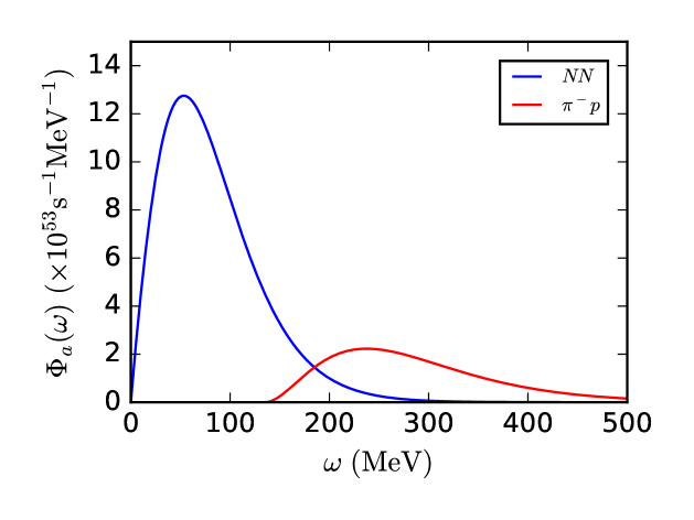
Figure 1: The spectra of the axion emitted from a SN, taking $\tilde{g}_{aNN}=5\times 10^{-10}$, $\kappa_{\rm SN}=3$, and $L_{a}^{(\pi^{-}p)}=L_{a}^{(NN)}$. The blue line is for the $NN$ process, which is calculated in our SN model. The red line is for the $\pi^{-1}p$ process, which is obtained from the fitting formula shown in Eq. (2.11).

As well as the $NN$ bremsstrahlung process, the $\pi^{-}p$ scattering process also produces the axion efficiently:

$$\pi^{-}+p\rightarrow n+a.$$ (2.10)

In many literatures, it has been expected that the axion production in the SN is dominated by the $NN$ bremsstrahlung process. However, recently, Refs. [36, 37] pointed out that the $\pi^{-}p$ scattering process is also important. The axion emissivity due to the $\pi^{-}p$ scattering process is comparable to that due to the $NN$ bremsstrahlung process and the axion spectrum from the $\pi^{-}p$ process is harder than that from the $NN$ bremsstrahlung process. For the $\pi^{-}p$ process, we assume that the axion spectrum is proportional to the one given in Ref. [36], which we found can be well approximated as

$$\Phi_{a}^{(\pi^{-}p)}(\omega)\propto(\omega-135\ {\rm MeV})^{2.07}\,e^{-0.0202\,(\omega/1\ {\rm MeV})}.$$ (2.11)

Because the axion luminosities due to the $NN$ and $\pi^{-}p$ processes are expected to be of the same order [36], we simply assume that the time-averaged luminosity due to the $\pi^{-}p$ process, denoted as $L_{a}^{(\pi^{-}p)}$, is equal to that due to the $NN$ bremsstrahlung process to determine the normalization of $\Phi_{a}^{(\pi^{-}p)}$. We use Eq. (2.11) to determine the (time-averaged) spectrum of the axion from the $\pi^{-}p$ process. In Fig. 1, we also show $\Phi_{a}^{(\pi^{-}p)}$, taking $L_{a}^{(\pi^{-}p)}=L_{a}^{(NN)}$. We can see that the spectrum is peaked at $\omega\sim 240\ {\rm MeV}$. Notice that, because the axion from the $\pi^{-}p$ process has harder spectrum, the number of axion from the $\pi^{-}p$ process is smaller than that from the $NN$ bremsstrahlung process if $L_{a}^{(\pi^{-}p)}\sim L_{a}^{(NN)}$.

The total number of axion emitted from the SN is calculated as

$$N_{a}=\dot{N}_{a}\Delta t_{\rm SN},$$ (2.12)

where $\Delta t_{\rm SN}$ is the post-bounce time when the axion emission becomes ineffective, and $\dot{N}_{a}$ is the axion emission rate:

$$\dot{N}_{a}\equiv\int d\omega\Phi_{a}(\omega),$$ (2.13)

with $\Phi_{a}\equiv\Phi_{a}^{(NN)}+\Phi_{a}^{(\pi^{-}p)}$.

Before closing this section, we summarize constraints on the axion couplings which will be used in the following discussion. In order not to affect the SN cooling too much, the effective axion-nucleon-nucleon coupling is bounded from above. In Ref. [12], the bound is given by $\tilde{g}_{aNN}\lesssim 9.1\times 10^{-10}$, assuming that the axion production is dominated by the $NN$ bremsstrahlung process. Here, because we also consider the $\pi^{-}p$ process with taking $L_{a}^{(\pi^{-}p)}\sim L_{a}^{(NN)}$, we adopt the following bound:

$$\tilde{g}_{aNN}\lesssim 6.4\times 10^{-10}.$$ (2.14)

The axion-photon-photon coupling $g_{a\gamma\gamma}$ is also bounded from above. The most stringent constraint on the axion-photon-photon coupling is given by the non-observation of the axion emission from the sun. The CAST experiment provides the upper bound on $g_{a\gamma\gamma}$ as [24]

$$g_{a\gamma\gamma}\lesssim 0.66\times 10^{-10}\ {\rm GeV}^{-1}.$$ (2.15)

3 Axion Conversion to Photon

Next, let us briefly review the conversion of the axion to photon in the presence of magnetic field [38, 39, 40]. Such a conversion process plays an essential role in observing the SN axion with collider detectors.

We are interested in the propagation of plane-wave axion and photon under the influence of static and uniform magnetic field. In such a situation, axion mixes with the photon whose polarization vector is in the plane containing the propagation direction and the direction of the magnetic field. (The amplitude of the photon with such a polarization is denoted as $A_{||}$). Considering the mode with the oscillation frequency $\omega$, Lagrangian given in Eq. (2.1) results in the following evolution equation of the axion $a$ and $A_{||}$ [40]:

$$\left(\begin{array}[]{cc}\omega^{2}+\partial_{L}^{2}&g_{a\gamma\gamma}B_{T}\omega\\ g_{a\gamma\gamma}B_{T}\omega&\omega^{2}+\partial_{L}^{2}-m_{a}^{2}\end{array}\right)\left(\begin{array}[]{c}A_{||}\\ a\end{array}\right)=0,$$ (3.5)

where $L$ denotes the propagation distance, and $B_{T}\equiv B\sin\theta$ with $\theta$ being the angle between the propagation direction and the direction of the magnetic field. (In collider detectors, the magnetic field is parallel to the beam axis and hence $\theta$ is the angle between the beam axis and the direction of the SN from the earth.) Using the fact that the dispersion relations of $a$ and $A_{||}$ are well approximated by $k\simeq\omega$ (with $k$ being the wave number), the above equation can be expressed as

$$i\partial_{L}\left(\begin{array}[]{c}A_{||}\\ a\end{array}\right)=\left(\begin{array}[]{cc}\omega&g_{a\gamma\gamma}B_{T}/2\\ g_{a\gamma\gamma}B_{T}/2&\omega-q\end{array}\right)\left(\begin{array}[]{c}A_{||}\\ a\end{array}\right),$$ (3.12)

where

$$q\equiv\frac{m_{a}^{2}}{2\omega}.$$ (3.13)

Numerically, $q^{-1}\simeq 4\ {\rm m}\times(\omega/10\ {\rm MeV})(m_{a}/1\ {\rm eV})^{-2}$.

Solving the above differential equation, the conversion probability from the axion to the photon is given by

$$P(L)=\frac{1}{4}(g_{a\gamma\gamma}B_{T}L)^{2}\left(\frac{\sin(qL/2)}{qL/2}\right)^{2}.$$ (3.14)

Notice that the conversion probability grows as $L^{2}$ as far as $L\lesssim q^{-1}$.

Now, we consider the conversion of the SN axion to the photon in collider detectors. Hereafter, we consider a detector with the conventional design such that a strong magnetic field is applied in the central region where detectors for the tracking are installed. We estimate the number of the photon converted from the SN axion assuming that the density of the material in the central region is so small that the scattering probability of $O(10-100)\ {\rm MeV}$ photon is negligible. Thus, in the central region of the detector, the photon is assumed to propagate (almost) freely; validity of this assumption will be considered later. The photon converted from the SN axion is expected to be observed by the ECAL surrounding the central region.

In calculating the number of photon converted from the SN axion, for simplicity, we approximate that the shape of the central region as a cylinder with the radius of $R$ and the length of $Z$ and that the magnetic field in the central region is uniform. Here, we consider the ATLAS and the CMS detectors of the LHC experiment and the ILD and the SiD detectors of the ILC experiment. The parameters characterizing these detectors are summarized in Table 2.

	$R$	$Z$	$B$	$\bar{L}(\theta=\frac{\pi}{6})$	$\bar{L}(\theta=\frac{\pi}{3})$	$\bar{L}(\theta=\frac{\pi}{2})$
ATLAS (LHC) [41]	$1.1\ {\rm m}$	$6.7\ {\rm m}$	$2.0\ {\rm T}$	$1.2\ {\rm m}$	$1.4\ {\rm m}$	$1.8\ {\rm m}$
CMS (LHC) [42]	$1.3\ {\rm m}$	$5.8\ {\rm m}$	$3.8\ {\rm T}$	$1.3\ {\rm m}$	$1.9\ {\rm m}$	$2.1\ {\rm m}$
ILD (ILC) [43]	$1.8\ {\rm m}$	$4.9\ {\rm m}$	$3.5\ {\rm T}$	$1.6\ {\rm m}$	$2.6\ {\rm m}$	$2.9\ {\rm m}$
SiD (ILC) [43]	$1.2\ {\rm m}$	$3.3\ {\rm m}$	$5.0\ {\rm T}$	$1.1\ {\rm m}$	$1.7\ {\rm m}$	$2.0\ {\rm m}$

Table 2: Detector parameters adopted in our analysis. The magnetic field of the ATLAS detector in the tracking volume deviates significantly from uniformity [41]; we take $B=2.0\ {\rm T}$ as an averaged magnetic field. We also show the effective path length for $\theta=\frac{\pi}{6}$, $\frac{\pi}{3}$, and $\frac{\pi}{2}$, for the case of $q\bar{L}\ll 1$.

For a given SN, the spectrum of the photon converted from the SN axion is given in the following form:

$$F_{\gamma}(\omega)=\frac{\Delta t_{\rm SN}}{4\pi d_{\rm SN}^{2}}\Phi_{a}(\omega)\int dAP(L_{A}).$$ (3.15)

The integration is over the cross-section area. The propagation length of the path inside the cylinder (i.e., the central region of the detector) is dependent on the cross-section area and is denoted as $L_{A}$; $P(L_{A})$ is the conversion probability for such a path.

In order to discuss the axion-photon conversion in detectors, we define the “effective path length” as follows:

$$\bar{L}\equiv\left[\frac{1}{2RZ}\int dA\,L_{A}^{2}\left(\frac{\sin(qL_{A}/2)}{qL_{A}/2}\right)^{2}\right]^{1/2}\sin\theta.$$ (3.16)

Notice that $2RZ$ is the total cross section area for $\theta=\frac{\pi}{2}$. In Table 2, $\bar{L}$ is also shown for several values of $\theta$ taking $q\rightarrow 0$. Using $\bar{L}$, the number of photon converted from the SN axion can be expressed as

$$N_{\gamma}=\,\frac{\dot{N}_{a}\Delta t_{\rm SN}}{8\pi d_{\rm SN}^{2}}RZ(g_{a\gamma\gamma}B\bar{L})^{2}.$$ (3.17)

Numerically, we find

$$N_{\gamma}\simeq \,25\times\left(\frac{2RZ}{15\ {\rm m^{2}}}\right)\left(\frac{\bar{L}}{2\ {\rm m}}\right)^{2}\left(\frac{B}{4\ {\rm T}}\right)^{2}$$

$$\,\times\left(\frac{\kappa_{\rm SN}}{3}\right)\left(\frac{d_{\rm SN}}{100\ {\rm pc}}\right)^{-2}\left(\frac{\Delta t_{\rm SN}}{10\ {\rm sec}}\right)\left(\frac{g_{a\gamma\gamma}}{7\times 10^{-11}\ {\rm GeV}^{-1}}\right)^{2}\left(\frac{\tilde{g}_{aNN}}{6\times 10^{-10}}\right)^{2}.$$ (3.18)

From Eq. (3.18), we can see that the number of the photon converted from the SN axion may be significant. Taking $g_{ann}=6.4\times 10^{-10}$, $g_{a\gamma\gamma}=6.6\times 10^{-11}\ {\rm GeV}^{-1}$, which correspond to the maximal possible values of the effective axion-nucleon-nucleon coupling and axion-photon-photon coupling, respectively (see Eqs. (2.14) and (2.15)), $d_{\rm SN}=77\ {\rm pc}$ (corresponding to the distance to Spica), $\kappa_{\rm SN}=3$, $\Delta t_{\rm SN}=10\ {\rm sec}$, and $\theta=\frac{\pi}{6}-\frac{\pi}{2}$, $N_{\gamma}$ can be as large as $4-8$, $16-43$, $25-81$, and $11-35$ for the ATLAS, CMS, ILD, and SiD setups, respectively. (For the case of the CMS, however, the axion-photon conversion may be affected by the materials in the central region, resulting in the suppression of the number of the signal; see the discussion below.)

We comment here that the signal photon converted from the SN axion enters only into (almost) a half of the ECAL. In our procedure, the ECAL can be geometrically divided into “upper” and “lower” halfs. The upper half is defined as the ECAL where the SN axion passes before entering into the central region, while the lower half is the rest of the ECAL. Then, the signal photon converted from the SN axion can be detected only in the lower half. This can be used to understand the background properties as we will discuss later.

4 Detection of the Signal of SN Axion

Now, we study the possibility of detecting the signal of the SN axion at collider detectors. It is highly non-trivial to identify the SN axion signal during the normal operation of the collier experiments. The signal photon may not be distinguished from photon (and other particles) produced by the beam collision. Thus a special procedure is necessary for the detection of the SN axion at the time of the SN, including the turn off of the beam.

For the detection of the SN axion signal, we use the fact that nearby SNe are expected to be alerted well in advance by the pre-SN neutrino alert. A large number of neutrinos are emitted at the time of the core collapse SN. The neutrino flux is regularly monitored by detectors which are sensitive to the SN neutrino, like KamLAND [44], SNO+ [45], and SuperKamiokande [46]. In the future, sensitivity to the nearby SNe can be strengthened by observatories like JUNO [47], Hyper-Kamiokande [48], and DUNE [49, 50, 51, 52]. These observatories form a global network to provide a prompt warning of a nearby SN when an anomalous increase of the neutrino flux, which indicates a nearby SN, is found. This global network is called the Supernova Early Warning System (SNEWS) [53, 54, 55]. The calculation of the neutrino flux [27, 56, 57, 58, 59, 60, 61, 62, 63, 64, 65] shows that, if a SN progenitor is located within $\sim 1~{}\rm{kpc}$, the neutrino emission is large enough to be detected even before the SN core collapse. Such an increase of the pre-SN neutrino makes it possible to forecast the SN which occur within $\sim O(100)\ {\rm pc}$; for $d_{\rm SN}\lesssim 200\ {\rm pc}$, an alert is possible $O(1-10)\ {\rm hours}$ before the core collapse [26, 27]. With the help of the pre-SN alert, we may know when the collider operation should be switched to the special one for the SN axion.

In the following, we first consider backgrounds. Then, we discuss the detectability of the signal at the ILC and LHC detectors.

4.1 Backgrounds

The most serious source of the background is expected to be the neutrino emitted by the SN of our interest. The neutrino emitted by the nearby SN should arrive simultaneously with the SN axion and it interacts with the material in the detector. Most importantly, the electron neutrino $\nu_{e}$ emitted from the SN interacts with heavy nuclei in the calorimeter via the charged current interaction and becomes electron. Such electron produced in the ECAL may mimic the signal photon.

For the estimation of the background rate, we use the fitting formula for the electron neutrino flux given in Ref. [66]:

$$f_{\nu_{e}}(E_{\nu})=\frac{L_{\nu_{e}}}{4\pi d_{\rm SN}^{2}\bar{E}_{\nu_{e}}^{2}}\frac{(\alpha_{e}+1)^{\alpha_{e}+1}}{\Gamma(\alpha_{e}+1)}\left(\frac{E_{\nu}}{\bar{E}_{\nu_{e}}}\right)^{\alpha_{e}}e^{-(\alpha_{e}+1)E_{\nu}/\bar{E}_{\nu_{e}}}.$$ (4.1)

Here, $L_{\nu_{e}}$ is the total luminosity, $\alpha_{e}$ is a positive constant of $O(1)$, and $\bar{E}_{\nu_{e}}$ is the averaged energy which is $\sim 10-15\ {\rm MeV}$. These parameters depend on time and we adopt the parameters for $t_{\rm pb}=1.991\ {\rm sec}$, i.e., $L_{\nu_{e}}=4.8\times 10^{51}\ {\rm erg/sec}$, $\alpha_{e}=2.92$, and $\bar{E}_{\nu_{e}}=10.01\ {\rm MeV}$, to evaluate the background rate.

As we will see below, the scattering rate due to the SN neutrino is much higher than the signal rate (which is at most $O(10)\ {\rm Hz}$). Thus, we should somehow remove the background due to the SN neutrino. For this purpose, we propose to use the difference of energy distributions of the SN axion and the SN neutrino. The signal photon and the background electron inherit the energy of the parent axion and neutrino, respectively. (In our analysis, for simplicity, the energy of the electron produced by the charged current process is approximated to be equal to that of the parent SN neutrino.) The energy of the electron produced by the SN neutrino is typically $\sim 10\ {\rm MeV}$, while the typical energy of the signal photon is higher. With imposing a cut on the energy deposit in the ECAL, we may remove the background.

The cosmic-ray muons may also leave some activity in the calorimeter. We expect that the muon detector, which is located at the most outer region of the detector, can be used as the veto counter to remove the cosmic-ray background. Thus, we neglect such a background.

4.2 Detection at the ILC detectors

First, we consider the ILC detectors which provide better environment for the SN axion detection than the LHC ones. In particular, we consider the case with the ILD, which has longer effective path length than the SiD, in detail. In the case of the ILD, the total radiation length up to the outside of the central tracker region is $\sim 0.1$ [43], and we may regard the photon as a freely propagating particle in the central region.

The ILC detectors are planned to have tungsten-based ECALs. For the ILD setup, the total depth of the tungsten is $8.4\ {\rm cm}$ (i.e., $24$ radiation length) to the radial direction, corresponding to the total weight of $\sim 120\ {\rm t}$ (equivalent to $\sim 4\times 10^{29}$ of tungsten atom). The SN neutrino, in particular, $\nu_{e}$, interacts with the tungsten in the ECAL via the charged current interaction. We could not find the cross section for such a background process, $\nu_{e}({\rm W},e^{-})X$, while the cross section of $\nu_{e}$ with lead, $\nu_{e}({\rm Pb},e^{-})X$, can be found in Ref. [66, 67] and is of order $10^{-41}-10^{-39}\ {\rm cm}^{2}$ for the neutrino energy of our interest. Based on the observation that the neutrino scattering cross section with nuclei tends to increase as the atomic number becomes larger, we presume that the scattering cross section for $\nu_{e}({\rm W},e^{-})X$ is at most comparable to (or smaller than) that for $\nu_{e}({\rm{}^{208}Pb},e^{-})X$. In estimating the background rate, we take the cross section for $\nu_{e}({\rm W},e^{-})X$ to be equal to that for $\nu_{e}({\rm{}^{208}Pb},e^{-})X$. We expect that such an approximation gives a conservative estimation of the background rate.

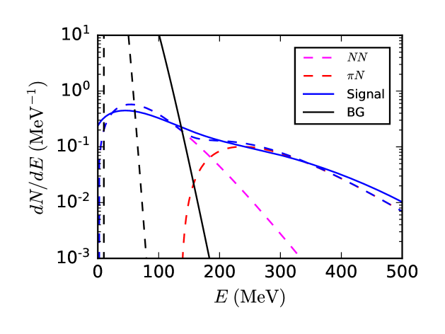
Figure 2: The spectrum of the signal and background events for the setup of the ILD, taking $\tilde{g}_{aNN}=6.4\times 10^{-10}$, $g_{a\gamma\gamma}=6.6\times 10^{-11}\ {\rm GeV}^{-1}$, $d_{\rm SN}=77\ {\rm pc}$, $\Delta t_{\rm SN}=10\ {\rm sec}$, $\kappa_{\rm SN}=3$, $\theta=\frac{\pi}{2}$, and $q^{-1}\gg\bar{L}$. Signal and background spectrum are shown in blue and gray lines, respectively. Solid lines represent the spectrum with taking into account the detector effect, while dashed lines represent non-smeared spectra.

In Fig. 2, we show in dashed lines the spectrum of the photon converted from the SN axion, as well as that of the electron due to the SN neutrino, for the ILD setup. We show the total signal with blue (dashed) line and the backgrounds with gray (dashed) line, while separately show the contribution from $NN$ bremsstrahlung process and pion-induced process. Here, we use the maximal possible values of $\tilde{g}_{aNN}=6.4\times 10^{-10}$ and $g_{a\gamma\gamma}=6.6\times 10^{-11}\ {\rm GeV}^{-1}$, and take $d_{\rm SN}=77\ {\rm pc}$, $\Delta t_{\rm SN}=10\ {\rm sec}$, $\kappa_{\rm SN}=3$ with $\theta=\pi/2$. With such a choice of parameters, the total number of the scattering event by the SN neutrino is $\sim 10^{5}$ and hence the rate is $\sim 10\ {\rm kHz}$.

Even though the number of the electron produced by the SN neutrino exponentially decreases when $E\gtrsim 10\ {\rm MeV}$ (with $E$ being the energy deposit in the ECAL), the observed background spectrum should have longer high energy tail because of the energy resolution of the ECAL. Here, we estimate the observed spectrum adopting the following energy resolution of the ILD detector [43]:

$$\frac{\delta E}{E}=\frac{15\%}{\sqrt{E_{\rm GeV}}},$$ (4.2)

where $E_{\rm GeV}$ is the energy in units of GeV. The smeared signal and background spectra are also shown in Fig. 2. We can see that the number of background can be significantly reduced if we require large enough $E$. We introduce $E_{\rm cut}$ such that

$$\int_{E_{\rm cut}}^{\infty}dE\left[\frac{dN_{\rm BG}}{dE}\right]_{\rm smeared}=1,$$ (4.3)

where $[dN_{\rm BG}/dE]_{\rm smeared}$ is the background spectrum after taking into account the detector resolution; for the present choice of parameters, $E_{\rm cut}\simeq 145\ {\rm MeV}$. Then, we regard the region $E>E_{\rm cut}$ as the signal region and define the number of signal as

$$N_{\rm signal}\equiv\int_{E_{\rm cut}}^{\infty}dE\left[\frac{dN_{\rm signal}}{dE}\right]_{\rm smeared},$$ (4.4)

with $[dN_{\rm signal}/dE]_{\rm smeared}$ being the photon spectrum with the effect of the detector resolution included.

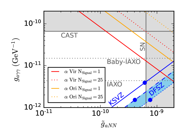
Figure 3: Contours of constant $N_{\rm signal}$ on $\tilde{g}_{ann}$ vs. $g_{a\gamma\gamma}$ plane for Spica ($\alpha$ Vir, red) and Betelgeuse ($\alpha$ Ori, orange), for the ILD setup. Here, we take $\Delta t_{\rm SN}=10\ {\rm sec}$, $\kappa_{\rm SN}=3$, $\theta=\frac{\pi}{2}$, and assume that $q^{-1}\gg\bar{L}$. The vertical line shows the upper bound on $\tilde{g}_{aNN}$ from the SN cooling [12] (See Eq. (2.14)). The solid and dotted horizontal lines indicate the CAST bound [24] and expected sensitivities of Baby-IAXO [68] and and IAXO [68], respectively, assuming $m_{a}\lesssim 10\ {\rm meV}$. The predictions of the QCD axion models in Eqs. (2.2) – (2.5) are shown in blue lines. (The solid line is for the KSVZ model, and dashed and dotted lines are for DFSZ model with $\tan\beta=0$ and $\infty$, respectively. The band in skyblue indicates the region predicted by the DFSZ model. The blobs on the blue lines indicate the point at which $m_{a}=10\ {\rm meV}$.)

In Fig. 3, we show the contour of constant $N_{\rm signal}$. On the same figure, we also show the parameter region excluded by the SN cooling or by the CAST experiment. We can see that, if $d_{\rm SN}\lesssim 200\ {\rm pc}$ (roughly corresponding to the distance to Betelgeuse), the number of signal can become $O(1)$ or larger in the parameter region which is still viable. We can see that, with the setup adopted in Fig. 3, it is difficult to reach the parameter region suggested by the QCD axion. However, wide variety of ALPs may show up in the string theory and the SN axion search of our proposal may be able to access some of those. In addition, the SN axion search of our proposal may also reach a part of parameter region covered by Baby-IAXO (and IAXO) experiment. Thus, if an ALP signal is found by Baby-IAXO, a joint analysis of the results of Baby-IAXO and the SN axion search (if performed) will give us deeper understanding of the ALP.

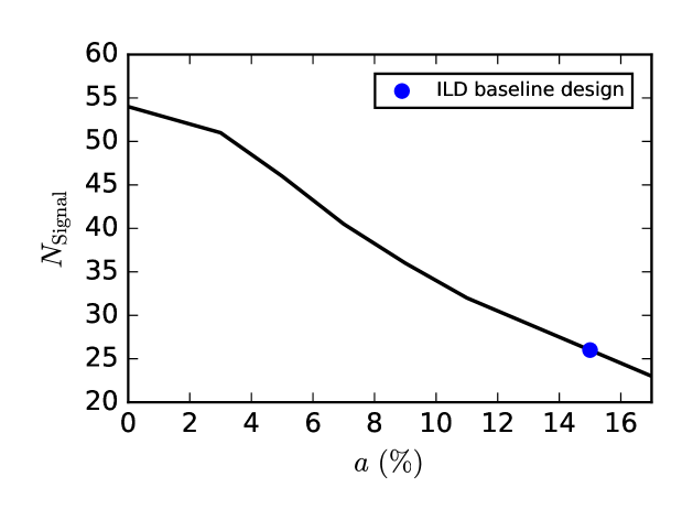
Figure 4: Number of signal as a function of the detector-resolution parameter $a$ (see Eq. (4.5)) for the case of the ILD setup except for the ECAL resolution. Here, we take $\tilde{g}_{aNN}=6.4\times 10^{-10}$, $g_{a\gamma\gamma}=6.6\times 10^{-11}\ {\rm GeV}^{-1}$, $d_{\rm SN}=77\ {\rm pc}$, $\Delta t_{\rm SN}=10\ {\rm sec}$, $\kappa_{\rm SN}=3$ and $\theta=\pi/2$.

As we have seen, the background spectrum is strongly affected by the detector resolution. If a better resolution than the one given in Eq. (4.2) is realized, we may reduce the number of background with lower $E_{\rm cut}$. We assume the following form of the detector resolution:

$$\frac{\delta E}{E}=\frac{a}{\sqrt{E_{\rm GeV}}},$$ (4.5)

and see how $N_{\rm signal}$ depends on the detector resolution with determining $E_{\rm cut}$ by solving Eq. (4.3). The number of signal increases with an ECAL with better resolution. With the ECAL based on ${\rm PbWO_{4}}$, which is used in the CMS, $a\sim 3\ \%$ can be realized [69]. With such an ECAL, for example, the number of signal can be increased by the factor of $\sim 2$ compared to the case with the tungsten-based ECAL.

So far, we have adopted axion and neutrino spectra calculated with assuming that the axion emission is subdominant for the SN cooling. If the axion-nucleon-nucleon coupling becomes large, significant amount of the energy is carried away by the axion and the cooling process of the SN is affected. The axion and neutrino spectra for the case of $L_{a}\sim L_{\nu}$ has been studied in Ref. [37]; if $L_{a}\sim L_{\nu}$, the axion spectrum may become softer than the one we adopt. With such a softer spectrum, the number of photon after imposing the cut may be reduced compared to our previous estimation. We have checked that, even if we use the axion spectrum given in Ref. [37], the number of signal event with $E\gtrsim E_{\rm cut}$ can be as large as a few for $d_{\rm SN}\sim 100\ {\rm pc}$.

One caveat for the case with the ILC is on the detector operation. In the ILC experiment, the bunches of $e^{+}$ and $e^{-}$ collide every $\sim 200\ {\rm millisec}$ and the bunch train is about $1\ {\rm millisec}$ long. For $\sim 199$ out of $200\ {\rm millisec}$, the detector is planned to be turned off in the normal operation (so-called “power-pulsing”). The SN axion search is hardly performed if the livetime is reduced down to $\sim 0.5\ \%$ as in the case of the normal operation. Thus, a special detector operation dedicated for the SN axion search is necessary. In particular, the detector (at least the ECAL) should be continuously turned on during the time window of the SN. In addition, the energy of the photon of our interest is $\sim 100\ {\rm MeV}$; the energy threshold of the ECAL should be low enough to detect such a photon. With the continuous operation of the detector, the power consumption may be an issue [43]. For the detection of the SN axion, the vertex and tracking detectors are irrelevant and they can be fully turned off, which may help to reduce the power consumption during the SN axion search.

4.3 Detection at the LHC detectors

Next, we comment on the LHC detectors, i.e., the ATLAS and the CMS.

As shown in Table 2, the ATLAS has weaker magnetic field and shorter effective path length than the CMS. The expected number of the signal event is small and the discovery of the signal of the axion emission is challenging at the ATLAS even with the most optimistic choices of the axion couplings and $d_{\rm SN}$. The CMS has stronger magnetic field than the ATLAS. A naive estimation of the number of signal based on Eq. (3.17) gives $N_{\gamma}\sim O(10)$ with the most optimistic choices of parameters. For the detection of the SN axion by the ATLAS or the CMS detector, if performed, a new trigger dedicated for the SN axion signal is necessary; the trigger should be replaced at the time of the pre-SN alert.

However, for the cases of the LHC detectors, the total amount of the material in the tracker region is sizable. From the beam pipe to the outside of the tracker region, the total material budget of the ATLAS detector is $\sim 0.3-2$ radiation length for $|\eta|=0-4$ (with $\eta$ being the pseudorapidity) in the high luminosity scenario of the LHC (HL-LHC) [70]. For the case of the CMS, it is $\sim 0.3-1.6$ radiation length for $|\eta|=0-1.5$ and $\sim 1.6-0.8$ radiation length for $|\eta|=1.5-3$ [71]. Thus, the photon may not be regarded as a free particle in the central region and the conversion rate of the SN axion to the photon is suppressed.

Another possibility to use the LHC detectors for the SN axion detection is to look for the photon originating from the SN axion using the $e^{+}e^{-}$ pair converted from the photon by the tracker material. Because of the relatively large material budget of the LHC inner detectors, the photon from the SN axion is, if produced, converted to the $e^{+}e^{-}$ pair with high probability, which may be regarded as a signal of the SN axion. The detailed calculation of the event rate of such $e^{+}e^{-}$ process is beyond the scope of this article and we leave it as future project.

5 Conclusions and Discussion

We have discussed the possibility to observe the axion emission from a nearby SN, which may occur in the future, using collider detectors. The axion produced in association with the SN event can be converted to the photon by the strong magnetic field in the central region of the detector and the photon can be detected by the ECAL surrounding the central region. We have calculated the number of signal event in existing and proposed detectors in the LHC and the ILC experiments. For the detection of the signal, a special collider operation dedicated for the SN axion signal is necessary at the time of a nearby SN which can be known in advance by the pre-SN alert:

1. At the time of the pre-SN alert, the beam should be stopped to make the detector environment quite.

2. The detector operation should be switched to the one dedicated for the SN axion search.

3. Then, we just have to wait for the SN axion to come. If a sizable number of photons are observed during the time window of the SN, it is an evidence of the axion emission from the SN.

We have seen that, with an optimistic choices of parameters, the ILC detectors may be used to observe the axion from a nearby SN. The SN axion search of our proposal may access ALPs suggested by string models, which are not excluded yet, while it is difficult to reach the parameter region of the QCD axion.

Several comments are in order:

• In the SN axion search of our proposal, only the “lower” half of the ECAL is used for the signal detection, and no signal is expected in the “upper” half. Thus, the study of the number of event in the “upper” half of ECAL will provide a reliable estimation of the background.

• So far, we have concentrated on the detection of the SN axion from a nearby SN. For such a purpose, the neutrino-induced event are regarded as background. However, the study of the neutrino-induced events may be also interesting. For example, with the collider detectors, we may obtain information about the energy spectrum of the neutrino (in particular, $\nu_{e}$). We may also learn the time-dependence of the neutrino emissivity from the SN. Such information, if obtained, can be used to acquire deep insights into the physics of the SN.

Our proposal of the SN axion detection is low-cost assuming that the change of the detector operation can be done at the software level. There is (almost) no effect on the regular program of the collider experiment. Thus, we suggest each detector collaboration to prepare in advance a detailed procedure for a nearby SN even though it rarely happens.

Acknowledgments: The authors are grateful to Yutaro Iiyama, Toshio Namba and Taikan Suehara for useful discussion and comments. This work was supported by JSPS KAKENHI Grant Nos. 20H01911 (SA), 16H06490 (TM), 18K03608 (TM), and 22H01215 (TM), and also by the JSPS Fellowship No. 21J20445 (YK).

References

- [1] R.D. Peccei and H.R. Quinn, CP Conservation in the Presence of Instantons, Phys. Rev. Lett. 38 (1977) 1440.
- [2] R.D. Peccei and H.R. Quinn, Constraints Imposed by CP Conservation in the Presence of Instantons, Phys. Rev. D 16 (1977) 1791.
- [3] S. Weinberg, A New Light Boson?, Phys. Rev. Lett. 40 (1978) 223.
- [4] F. Wilczek, Problem of Strong and Invariance in the Presence of Instantons, Phys. Rev. Lett. 40 (1978) 279.
- [5] P. Svrcek and E. Witten, Axions In String Theory, JHEP 06 (2006) 051 [hep-th/0605206].
- [6] A. Arvanitaki, S. Dimopoulos, S. Dubovsky, N. Kaloper and J. March-Russell, String Axiverse, Phys. Rev. D 81 (2010) 123530 [0905.4720].
- [7] M. Cicoli, M. Goodsell and A. Ringwald, The type IIB string axiverse and its low-energy phenomenology, JHEP 10 (2012) 146 [1206.0819].
- [8] Particle Data Group collaboration, Review of Particle Physics, PTEP 2020 (2020) 083C01.
- [9] M.S. Turner, Axions from SN 1987a, Phys. Rev. Lett. 60 (1988) 1797.
- [10] G.G. Raffelt, Astrophysical axion bounds, Lect. Notes Phys. 741 (2008) 51 [hep-ph/0611350].
- [11] J.H. Chang, R. Essig and S.D. McDermott, Supernova 1987A Constraints on Sub-GeV Dark Sectors, Millicharged Particles, the QCD Axion, and an Axion-like Particle, JHEP 09 (2018) 051 [1803.00993].
- [12] P. Carenza, T. Fischer, M. Giannotti, G. Guo, G. Martínez-Pinedo and A. Mirizzi, Improved axion emissivity from a supernova via nucleon-nucleon bremsstrahlung, JCAP 10 (2019) 016 [1906.11844].
- [13] K. Hamaguchi, N. Nagata, K. Yanagi and J. Zheng, Limit on the Axion Decay Constant from the Cooling Neutron Star in Cassiopeia A, Phys. Rev. D 98 (2018) 103015 [1806.07151].
- [14] L.B. Leinson, Impact of axions on the Cassiopea A neutron star cooling, JCAP 09 (2021) 001 [2105.14745].
- [15] M. Buschmann, C. Dessert, J.W. Foster, A.J. Long and B.R. Safdi, Upper Limit on the QCD Axion Mass from Isolated Neutron Star Cooling, 2111.09892.
- [16] G.G. Raffelt, J. Redondo and N. Viaux Maira, The meV mass frontier of axion physics, Phys. Rev. D 84 (2011) 103008 [1110.6397].
- [17] A. Ayala, I. Domínguez, M. Giannotti, A. Mirizzi and O. Straniero, Revisiting the bound on axion-photon coupling from Globular Clusters, Phys. Rev. Lett. 113 (2014) 191302 [1406.6053].
- [18] M. Giannotti, I. Irastorza, J. Redondo and A. Ringwald, Cool WISPs for stellar cooling excesses, JCAP 05 (2016) 057 [1512.08108].
- [19] M. Giannotti, I.G. Irastorza, J. Redondo, A. Ringwald and K. Saikawa, Stellar Recipes for Axion Hunters, JCAP 10 (2017) 010 [1708.02111].
- [20] K. Saikawa and T.T. Yanagida, Stellar cooling anomalies and variant axion models, JCAP 03 (2020) 007 [1907.07662].
- [21] L. Di Luzio, M. Fedele, M. Giannotti, F. Mescia and E. Nardi, Stellar evolution confronts axion models, JCAP 02 (2022) 035 [2109.10368].
- [22] J. Engel, D. Seckel and A.C. Hayes, Emission and detectability of hadronic axions from SN1987A, Phys. Rev. Lett. 65 (1990) 960.
- [23] T. Moroi and H. Murayama, Axionic hot dark matter in the hadronic axion window, Phys. Lett. B 440 (1998) 69 [hep-ph/9804291].
- [24] CAST collaboration, New CAST Limit on the Axion-Photon Interaction, Nature Phys. 13 (2017) 584 [1705.02290].
- [25] S.-F. Ge, K. Hamaguchi, K. Ichimura, K. Ishidoshiro, Y. Kanazawa, Y. Kishimoto et al., Supernova-scope for the Direct Search of Supernova Axions, JCAP 11 (2020) 059 [2008.03924].
- [26] M. Mukhopadhyay, C. Lunardini, F.X. Timmes and K. Zuber, Presupernova neutrinos: directional sensitivity and prospects for progenitor identification, Astrophys. J. 899 (2020) 153 [2004.02045].
- [27] C. Kato, K. Ishidoshiro and T. Yoshida, Theoretical prediction of presupernova neutrinos and their detection, Ann. Rev. Nucl. Part. Sci. 70 (2020) 121 [2006.02519].
- [28] F. van Leeuwen, Validation of the new Hipparcos reduction, Astron. Astrophys. 474 (2007) 653 [0708.1752].
- [29] G.M. Harper, A. Brown, E.F. Guinan, E. O’Gorman, A.M.S. Richards, P. Kervella et al., An updated 2017 astrometric solution for betelgeuse, The Astronomical Journal 154 (2017) 11.
- [30] A.G.A. Brown, A. Vallenari, T. Prusti, J. de Bruijne, C. Babusiaux, C.A.L. Bailer-Jones et al., Gaia data release 2, Astronomy & Astrophysics (2018) .
- [31] G. Grilli di Cortona, E. Hardy, J. Pardo Vega and G. Villadoro, The QCD axion, precisely, JHEP 01 (2016) 034 [1511.02867].
- [32] J.E. Kim, Weak Interaction Singlet and Strong CP Invariance, Phys. Rev. Lett. 43 (1979) 103.
- [33] M.A. Shifman, A.I. Vainshtein and V.I. Zakharov, Can Confinement Ensure Natural CP Invariance of Strong Interactions?, Nucl. Phys. B 166 (1980) 493.
- [34] M. Dine, W. Fischler and M. Srednicki, A Simple Solution to the Strong CP Problem with a Harmless Axion, Phys. Lett. B 104 (1981) 199.
- [35] A.R. Zhitnitsky, On Possible Suppression of the Axion Hadron Interactions. (In Russian), Sov. J. Nucl. Phys. 31 (1980) 260.
- [36] P. Carenza, B. Fore, M. Giannotti, A. Mirizzi and S. Reddy, Enhanced Supernova Axion Emission and its Implications, Phys. Rev. Lett. 126 (2021) 071102 [2010.02943].
- [37] T. Fischer, P. Carenza, B. Fore, M. Giannotti, A. Mirizzi and S. Reddy, Observable signatures of enhanced axion emission from protoneutron stars, Phys. Rev. D 104 (2021) 103012 [2108.13726].
- [38] P. Sikivie, Experimental Tests of the Invisible Axion, Phys. Rev. Lett. 51 (1983) 1415.
- [39] P. Sikivie, Detection Rates for ’Invisible’ Axion Searches, Phys. Rev. D 32 (1985) 2988.
- [40] G. Raffelt and L. Stodolsky, Mixing of the Photon with Low Mass Particles, Phys. Rev. D 37 (1988) 1237.
- [41] ATLAS collaboration, ATLAS: Detector and physics performance technical design report. Volume 1, .
- [42] CMS collaboration, CMS Physics: Technical Design Report Volume 1: Detector Performance and Software, .
- [43] H. Abramowicz et al., The International Linear Collider Technical Design Report - Volume 4: Detectors, 1306.6329.
- [44] KamLAND collaboration, KamLAND Sensitivity to Neutrinos from Pre-Supernova Stars, Astrophys. J. 818 (2016) 91 [1506.01175].
- [45] SNO+ collaboration, Current Status and Future Prospects of the SNO+ Experiment, Adv. High Energy Phys. 2016 (2016) 6194250 [1508.05759].
- [46] Super-Kamiokande collaboration, Sensitivity of Super-Kamiokande with Gadolinium to Low Energy Anti-neutrinos from Pre-supernova Emission, Astrophys. J. 885 (2019) 133 [1908.07551].
- [47] JUNO collaboration, JUNO Conceptual Design Report, 1508.07166.
- [48] Hyper-Kamiokande collaboration, Hyper-Kamiokande Design Report, 1805.04163.
- [49] DUNE collaboration, Long-Baseline Neutrino Facility (LBNF) and Deep Underground Neutrino Experiment (DUNE): Conceptual Design Report, Volume 1: The LBNF and DUNE Projects, 1601.05471.
- [50] DUNE collaboration, Long-Baseline Neutrino Facility (LBNF) and Deep Underground Neutrino Experiment (DUNE): Conceptual Design Report, Volume 2: The Physics Program for DUNE at LBNF, 1512.06148.
- [51] DUNE collaboration, Long-Baseline Neutrino Facility (LBNF) and Deep Underground Neutrino Experiment (DUNE): Conceptual Design Report, Volume 3: Long-Baseline Neutrino Facility for DUNE June 24, 2015, 1601.05823.
- [52] DUNE collaboration, Long-Baseline Neutrino Facility (LBNF) and Deep Underground Neutrino Experiment (DUNE): Conceptual Design Report, Volume 4 The DUNE Detectors at LBNF, 1601.02984.
- [53] P. Antonioli et al., SNEWS: The Supernova Early Warning System, New J. Phys. 6 (2004) 114 [astro-ph/0406214].
- [54] K. Scholberg, The SuperNova Early Warning System, Astron. Nachr. 329 (2008) 337 [0803.0531].
- [55] SNEWS collaboration, SNEWS: The supernova early warning system, J. Phys. Conf. Ser. 309 (2011) 012026.
- [56] A. Odrzywolek, M. Misiaszek and M. Kutschera, Detection possibility of the pair - annihilation neutrinos from the neutrino - cooled pre-supernova star, Astropart. Phys. 21 (2004) 303 [astro-ph/0311012].
- [57] A. Odrzywolek, M. Misiaszek and M. Kutschera, Neutrinos from pre-supernova star, Acta Phys. Polon. B 35 (2004) 1981 [astro-ph/0405006].
- [58] M. Kutschera, A. Odrzywołek and M. Misiaszek, Presupernovae as Powerful Neutrino Sources, Acta Physica Polonica B 40 (2009) 3063.
- [59] A. Odrzywolek, Nuclear statistical equilibrium neutrino spectrum, Phys. Rev. C80 (2009) 045801 [0903.2311].
- [60] C. Kato, M.D. Azari, S. Yamada, K. Takahashi, H. Umeda, T. Yoshida et al., Pre-supernova neutrino emissions from ONe cores in the progenitors of core-collapse supernovae: are they distinguishable from those of Fe cores?, Astrophys. J. 808 (2015) 168 [1506.02358].
- [61] K.M. Patton, C. Lunardini and R.J. Farmer, Presupernova neutrinos: realistic emissivities from stellar evolution, Astrophys. J. 840 (2017) 2 [1511.02820].
- [62] T. Yoshida, K. Takahashi, H. Umeda and K. Ishidoshiro, Presupernova neutrino events relating to the final evolution of massive stars, Phys. Rev. D93 (2016) 123012 [1606.04915].
- [63] K.M. Patton, C. Lunardini, R.J. Farmer and F.X. Timmes, Neutrinos from beta processes in a presupernova: probing the isotopic evolution of a massive star, Astrophys. J. 851 (2017) 6 [1709.01877].
- [64] C. Kato, H. Nagakura, S. Furusawa, K. Takahashi, H. Umeda, T. Yoshida et al., Neutrino emissions in all flavors up to the pre-bounce of massive stars and the possibility of their detections, Astrophys. J. 848 (2017) 48 [1704.05480].
- [65] G. Guo, Y.-Z. Qian and A. Heger, Presupernova neutrino signals as potential probes of neutrino mass hierarchy, Phys. Lett. B796 (2019) 126 [1906.06839].
- [66] I. Tamborra, B. Muller, L. Hudepohl, H.-T. Janka and G. Raffelt, High-resolution supernova neutrino spectra represented by a simple fit, Phys. Rev. D 86 (2012) 125031 [1211.3920].
- [67] E. Kolbe and K. Langanke, The Role of neutrino induced reactions on lead and iron in neutrino detectors, Phys. Rev. C 63 (2001) 025802 [nucl-th/0003060].
- [68] IAXO collaboration, Physics potential of the International Axion Observatory (IAXO), JCAP 06 (2019) 047 [1904.09155].
- [69] CMS collaboration, Energy Calibration and Resolution of the CMS Electromagnetic Calorimeter in Collisions at TeV, JINST 8 (2013) P09009 [1306.2016].
- [70] C. Gemme, The ATLAS Tracker Detector for HL-LHC, ATL-ITK-PROC-2020-008.
- [71] CMS Tracker collaboration, The Upgrade of the CMS Tracker at HL-LHC, JPS Conf. Proc. 34 (2021) 010006 [2102.06074].