Spectral function of chiral one-dimensional Fermi liquid in the regime of strong interactions

Abstract

We study momentum-resolved tunneling into a system of spinless chiral one-dimensional fermions, such as electrons at the edge of an integer quantum Hall system. Interactions between particles give rise to broadening of the spectral function of the system. We develop an approach that enables one to obtain the shape of the peak in the spectral function in the regime of strong interaction. We apply our technique to the special cases of short-range and Coulomb interactions.

Low energy properties of one-dimensional systems of fermions are strongly affected by interactions between them. These systems are commonly described in terms of the Luttinger liquid theory [1, 2]. The signature feature of the Luttinger liquid is the power-law behavior of the tunneling density of states at low energies [3, 4]. A special kind of one-dimensional system—the chiral Luttinger liquid—has been predicted to emerge at the edge of the fractional quantum Hall system [5]. Its properties are controlled by the nature of the quantum Hall state; specifically, its occupation fraction $\nu$. For systems where $\nu^{-1}$ is odd integer, the tunneling density of states scales as a power of energy, $D(\epsilon)\propto\epsilon^{\alpha}$, with the exponent $\alpha=\nu^{-1}-1$ [5, 6]. Importantly, even though the interactions are crucial for the formation of the fractional quantum Hall state, their strength does not affect the value of the exponent $\alpha$.

In this paper we study the model of spinless chiral one-dimensional fermions, which can be realized experimentally as the edge mode of an integer quantum Hall system with occupation fraction $\nu=1$ [7]. The above results can be applied to this special case and yield the exponent $\alpha=0$, i.e., the density of states at the Fermi level assumes a constant value. This conclusion applies regardless of the strength of interaction between the fermions, and in this respect the system behaves as a Fermi rather than Luttinger liquid. The latter statement does not imply that the elementary excitations of the system are fermions. Their nature depends on momentum and interaction strength. In particular, in the case of Coulomb repulsion the low energy excitations are bosons [8].

Although interactions between fermions in this model do not lead to power-law scaling of the tunneling density of states, they manifest themselves in the spectral function of the system $A_{p}(\epsilon)$. The latter describes momentum-resolved tunneling into the system and provides more detailed information than the density of states $D(\epsilon)$. In the absence of interaction between particles, the spectral function has a sharp peak at the energy $\epsilon_{p}$ of the fermion of momentum $p$, i.e., $A_{p}(\epsilon)=\delta(\epsilon-\epsilon_{p})$. Interactions result in broadening of this peak. Our particular focus will be on the limit of strong interactions, where the elementary excitations with momenta of order $p$ are bosonic. Our main result is the exact shape of the peak in the spectral function in this regime.

Our approach to the evaluation of $A_{p}(\epsilon)$ is complementary to that developed for non-chiral systems in Ref. [9]. The latter applies at any interaction strength, but is limited to the evaluation of the spectral function only at the edge of support, where $A_{p}(\epsilon)$ exhibits power-law scaling. Our approach gives $A_{p}(\epsilon)$ for all energies, but is limited to the regime of strong interactions.

It is worth pointing out that the chiral nature of our problem ensures that for short-range interaction the spectral function vanishes outside of a finite interval of energies. Assuming that interactions are repulsive, the lower edge of support is analogous to that considered for the non-chiral case in Ref. [9], and there the results can be compared. On the other hand, the upper edge of support of $A_{p}(\epsilon)$ is qualitatively different and cannot be treated using the method of Ref. [9]. The fermion tunneling into the system near that energy generates a very large number of bosonic excitations. The corresponding physics is similar to that of the multiphonon spectrum of liquid helium [10] and multiparticle production in quantum field theory [11]. Finally, our approach is not limited to the case of short-range interactions. As an example, we also consider the case of Coulomb interactions, whose long-range nature changes the spectral function qualitatively.

We describe our system by the Hamiltonian $\hat{H}=\hat{H}_{0}+\hat{V}$, where

$$\hat{H}_{0} = \sum_{p}\epsilon_{p}c_{p}^{\dagger}c_{p},\quad\epsilon_{p}=vp+\frac{p^{2}}{2m}+\ldots,$$ (1)

$$\hat{V} = \frac{1}{L}\sum_{\begin{subarray}{c}p_{1}p_{2}\\ q>0\end{subarray}}V(q)c_{p_{1}+q}^{\dagger}c_{p_{1}}c_{p_{2}}^{\dagger}c_{p_{2}+q}.$$ (2)

Here $c_{p}$ is the fermion annihilation operator. The energy of the fermion $\epsilon_{p}$ is assumed to be a monotonic function of momentum $p$, which ensures that the fermions are chiral. The momentum and energy are measured from their values at the Fermi point. The system has a finite length $L$; we assume periodic boundary conditions. $V(q)$ is the Fourier transform of the interaction potential.

Our main interest is the spectral function of the system defined as

$$A_{p}(\epsilon)=\sum_{j}|\langle j|c_{p}^{\dagger}|0\rangle|^{2}\delta(\epsilon-E_{j}).$$ (3)

Here $|0\rangle$ denotes the eigenstate of $\hat{H}$ in which all single-particle states with $p<0$ are filled and those with $p\geq 0$ empty. The summation is over all the eigenstates $|j\rangle$ of the Hamiltonian $\hat{H}$, and $E_{j}$ is the energy of the state $|j\rangle$ measured from that of the vacuum state $|0\rangle$.

In the absence of interactions, the sum in Eq. (3) contains only one nonvanishing term, which corresponds to $|j\rangle=c_{p}^{\dagger}|0\rangle$. In this case we immediately obtain $A_{p}(\epsilon)=\delta(\epsilon-\epsilon_{p})$. In an interacting system, multiple eigenstates of the Hamiltonian $\hat{H}=\hat{H}_{0}+\hat{V}$ overlap with $c_{p}^{\dagger}|0\rangle$, and the spectral function $A_{p}(\epsilon)$ has the meaning of the distribution function of the energy of the system after a single fermion with momentum $p$ is added to it.

The width of the energy distribution can be quantified by evaluating its variance $\delta\epsilon^{2}=\overline{\epsilon^{2}}-\overline{\epsilon}^{2}$, where the averaging is performed by integrating with the weight $A_{p}(\epsilon)$. Using the definition (3), it can be expressed as

$$\delta\epsilon^{2}=\langle 0|c_{p}\hat{H}^{2}c_{p}^{\dagger}|0\rangle-\langle 0|c_{p}\hat{H}c_{p}^{\dagger}|0\rangle^{2}.$$ (4)

Substituting $\hat{H}=\hat{H}_{0}+\hat{V}$ given by Eqs. (1) and (2), in the thermodynamic limit $L\to\infty$ we find

$$\delta\epsilon^{2}=\frac{1}{8\pi^{2}\hbar^{2}}\int_{0}^{p}dq\int_{p-q}^{p}dq^{\prime}[V(q)-V(q^{\prime})]^{2}.$$ (5)

To illustrate our results, we will apply them to two types of interaction potential. First, we will consider short-range interactions that fall off with the distance fast enough to ensure that $V(q)$ and its second derivative $V^{\prime\prime}(q)$ are well defined at $q=0$. In this case we will approximate

$$V(q)=V(0)-\eta q^{2},\quad\eta=-\frac{1}{2}V^{\prime\prime}(0).$$ (6)

For simplicity, we will assume $\eta>0$, which corresponds to a typical repulsive interaction. Substituting this expression into Eq. (5), we obtain

$$\delta\epsilon^{2}=\frac{11}{720\pi^{2}\hbar^{2}}\eta^{2}p^{6}.$$ (7)

In addition, we will consider Coulomb interaction $e^{2}/|x|$ cut off at a short distance $w$. In this case we have

$$V(q)=2e^{2}\ln\frac{\hbar}{|q|w}$$ (8)

and

$$\delta\epsilon^{2}=\left(\frac{1}{\pi^{2}}-\frac{1}{12}\right)\frac{e^{4}p^{2}}{\hbar^{2}}.$$ (9)

It is worth mentioning that the expression (5) for the variance of the energy distribution and the subsequent results (7) and (9) are not pertubative in $\hat{V}$; they apply for any interaction strength.

Let us now discuss the effect of different parts of the Hamiltonian $\hat{H}$ on the spectral function. At small $p$ the largest contribution is $\sum_{p}vpc_{p}^{\dagger}c_{p}$, obtained from Eq. (1) by linearizing the energy spectrum, $\epsilon_{p}=vp$. This term is simply $v\hat{P}$, where $\hat{P}$ is the momentum operator. In our system, momentum is conserved, and $v\hat{P}$ commutes with the remaining terms of the Hamiltonian. Its effect on the spectral function (3) amounts to adding $vp$ to the energy of each state $|j\rangle$, and thus to the shift $vp$ of the peak in $A_{p}(\epsilon)$ as a function of energy at a given $p$. Importantly, this term does not affect the shape of the peak.

The leading term describing the curvature of the spectrum $\epsilon_{p}$ in Eq. (1) is $\delta\hat{H}_{0}=\sum_{p}(p^{2}/2m)c_{p}^{\dagger}c_{p}$. It does not commute with the interaction term $\hat{V}$. As a result, the evaluation of the spectral function in the regime where $\delta\hat{H}_{0}$ and $\hat{V}$ have comparable effects on it, is a challenging problem. To make further progress, we determine which of the two contributions to the Hamiltonian, $\delta\hat{H}_{0}$ or $\hat{V}$, is dominant at a given $p$ and interaction strength.

If the interactions are neglected, the effect of $\delta\hat{H}_{0}$ on the spectral function amounts to the additional shift of the peak by $\delta\epsilon_{p}=p^{2}/2m$. On the other hand, the interaction $\hat{V}$ results in broadening of the peak, with the characteristic width $\delta\epsilon$ given by Eq. (5). Comparison of $\delta\epsilon_{p}$ and $\delta\epsilon$ indicates which of the two perturbations gives the dominant contribution to $A_{p}(\epsilon)$. At $\delta\epsilon_{p}\gg\delta\epsilon$ the effect of interactions is small, and $\hat{V}$ can be accounted for in perturbation theory [12]. Below we study in detail the opposite case, $\delta\epsilon\gg\delta\epsilon_{p}$, in which the shape of the spectral function $A_{p}(\epsilon)$ is controlled by interactions. For short-range interactions, using Eq. (7) we find that the interaction dominated regime is achieved at $m\eta p/\hbar\gg 1$. For the Coulomb interaction, Eq. (9) yields the condition $me^{2}/\hbar p\gg 1$. Note that while for the short-range interactions the condition requires relatively high momentum $p\gg\hbar/m\eta$, in the Coulomb case interactions dominate at small momentum, $p\ll me^{2}/\hbar$.

The treatment of the problem in the limit of strong interactions is greatly simplified by bosonizing fermion operators. In the bosonic representation the state of the system is described by occupation numbers of bosonic states numbered by $l=1,2,\ldots$ and the total number of fermions $N$, which can be measured from that in the ground state $|0\rangle$. The fermion field operator is given by [1]

$$\Psi(x)=\frac{1}{\sqrt{L}}Ue^{ik_{F}x}e^{i\varphi^{\dagger}(x)}e^{i\varphi(x)}.$$ (10)

Here $k_{F}$ is the Fermi wavevector for a given number of particles $N$, the operator $U$ lowers $N$ by 1, and $\varphi(x)$ is related to the bosonic destruction operators $b_{l}$ by

$$\varphi(x)=-i\sum_{l=1}^{\infty}\frac{1}{\sqrt{l}}e^{iq_{l}x/\hbar}b_{l},\quad q_{l}=\frac{2\pi\hbar}{L}l.$$ (11)

The advantage of using bosonization is that for fermions with linear spectrum, $\epsilon_{p}=vp$, the Hamiltonian (1), (2) takes the simple form

$$\hat{H}_{b}=\sum_{l}\varepsilon_{l}b_{l}^{\dagger}b_{l},\qquad\varepsilon_{l}=\left(v+\frac{V(q_{l})}{2\pi\hbar}\right)q_{l}.$$ (12)

Importantly, $\hat{H}_{b}$ is quadratic in the bosonic operators, i.e., it describes a system of noninteracting bosonic elementary excitations with energies $\varepsilon_{l}$. The effects of the curvature of the spectrum would generate interactions of the bosons. From now on we limit ourselves to the strong interaction limit and thus neglect these interactions.

We start by rewriting the definition (3) of the spectral function in terms of the fermionic Green’s function,

$$A_{p_{k}}(\epsilon)=\int_{-\infty}^{\infty}\frac{dt}{2\pi\hbar}\int_{0}^{L}dx\,e^{-i(p_{k}x-\epsilon t)/\hbar}g(x,t),$$ (13)

where $g(x,t)=\langle 0|\Psi(x,t)\Psi^{\dagger}(0,0)|0\rangle$. To account for the finite size $L$ of the system, we replaced $p\to p_{k}=2\pi\hbar k/L$, where $k$ is integer. Given the simple quadratic form of the Hamiltonian (12) and the bosonized form (10) of the operator $\Psi$, the evaluation of the Green’s function is straightforward,

$$g(x,t)=\frac{1}{L}\exp\left(\sum_{l=1}^{\infty}\frac{1}{l}e^{i(q_{l}x-\varepsilon_{l}t)/\hbar}\right).$$ (14)

Expansion of the exponential in Eq. (14) in Taylor series upon substitution into Eq. (13) immediately yields

$$A_{p_{k}}(\epsilon) = 0,\quad k<0,$$ (15)

$$A_{p_{0}}(\epsilon) = \delta(\epsilon),$$ (16)

$$A_{p_{k}}(\varepsilon) = \sum_{\{N_{l}\}_{k}}\!\delta\Bigg{(}\epsilon-\sum_{l=1}^{\infty}N_{l}\varepsilon_{l}\Bigg{)}\!\prod_{l=1}^{k}\frac{1}{N_{l}!\,l^{N_{l}}},\quad k>0.\hskip 20.00003pt$$ (17)

Equation (15) is expected because in $|0\rangle$ all the fermion states with negative momenta are filled. The single $\delta$-function on the right-hand side of Eq. (16) accounts for the only possible state of the system with extra particle and momentum $0$. For $k>0$ the state $c_{p_{k}}^{\dagger}|0\rangle$ is a superposition of all possible states involving bosons with $l=1,2,\ldots,k$ and occupation numbers $N_{l}$, such that $\sum_{l}N_{l}l=k$, as required by momentum conservation. Thus, the summation in Eq. (17) is over all integer partitions of $k$.

As $k$ increases, the number of terms in Eq. (17), which is the number of integer partitions of $k$, grows exponentially [13]. Physically, we are interested in the thermodynamic limit, whereby $L\to\infty$ and $k\to\infty$ so that $p_{k}=2\pi\hbar k/L$ takes a fixed value $p$. It is not immediately clear how to take this limit in Eq. (17). Instead, we return to Eq. (13), replace $e^{-ip_{k}x/\hbar}\to(i\hbar/p_{k})\partial_{x}e^{-ip_{k}x/\hbar}$, and integrate by parts with respect to $x$. Using Eq. (14) we then find

$$A_{p_{k}}(\epsilon)=\frac{1}{k}\sum_{l=1}^{k}A_{p_{k-l}}(\epsilon-\varepsilon_{l}).$$ (18)

Here we limited the summation to $l\leq k$ because $A_{p_{k-l}}=0$ at $l>k$, see Eq. (15). Equation (18) is a recurrence relation that enables one to obtain the spectral function for any positive $k$, given known expressions for $k^{\prime}=0,1,\ldots,k-1$. In the thermodynamic limit we convert the sum in Eq. (18) into an integral and find

$$A_{p}(\epsilon)=\frac{1}{p}\int_{0}^{p}dqA_{p-q}(\epsilon-\varepsilon(q)),\quad\varepsilon(q)=\left(v+\frac{V(q)}{2\pi\hbar}\right)q.$$ (19)

For a given interaction $V(q)$, the spectral function can be found by solving the integral equation (19).

We now use Eq. (19) to evaluate $A_{p}(\epsilon)$ in the case of short-range interactions. Using Eq. (6), we get

$$\varepsilon(q)=\tilde{v}q-\frac{\eta}{2\pi\hbar}q^{3},\qquad q>0,$$ (20)

where $\tilde{v}=v+V(0)/2\pi\hbar$. Because the function $\varepsilon(q)$ is concave, the total energy $\epsilon$ of any set of bosonic excitations with the total momentum $p$ is in the range $\varepsilon(p)\leq\epsilon<\tilde{v}p$. Thus, it is convenient to look for a solution of the integral equation (19) in the form

$$A_{p}(\epsilon)=\frac{2\pi\hbar}{\eta p^{3}}a\left(\frac{2\pi\hbar}{\eta p^{3}}[\epsilon-\varepsilon(p)]\right),$$ (21)

where $a(\lambda)$ is a dimensionless function that vanishes outside the interval $0\leq\lambda<1$ and satisfies the normalization condition $\int_{0}^{1}a(\lambda)d\lambda=1$. Substitution of Eqs. (20) and (21) into Eq. (19) yields

$$a(\lambda)=\int_{0}^{1}\frac{d\zeta}{\zeta^{3}}a\left(\frac{\lambda-3\zeta(1-\zeta)}{\zeta^{3}}\right),$$ (22)

where introduced the integration variable $\zeta=(p-q)/p$.

A numerical solution of the integral equation (22) is shown in Fig. 1. A careful examination of Eq. (22) shows [14] that $a(0^{+})=1/3$, whereas at $\lambda\to 1$ the solution is suppressed exponentially,

$$\ln a(\lambda)\simeq-\frac{1}{2\sqrt{1-\lambda}}\ln\frac{1}{1-\lambda},\quad\lambda\to 1^{-}.$$ (23)

Near the lower edge of support the spectral function is expected to show power-law scaling with the exponent $\mu$, which depends on the interaction strength [9]. For the chiral system the result in the limit of strong interaction is $\mu=0$ [14], which is consistent with our conclusion that $a(\lambda)$ approaches a finite value at $\lambda\to 0^{+}$. In order for the state with momentum $p$ to have energy close to $\tilde{v}p$, corresponding to $\lambda=1$, the momentum must be distributed among a very large number of bosonic excitations. The amplitude of such processes is known [10, 11] to be exponentially suppressed in a way consistent with Eq. (23).

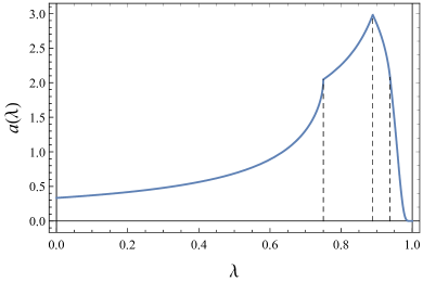
Figure 1: The dimensionless spectral function $a(\lambda)$ in the case of short-range interactions, obtained by solving the integral equation (22) numerically. The dashed lines are at $\lambda=\frac{3}{4},\frac{8}{9},\frac{15}{16}$.

In the case of Coulomb interaction, the energies of the bosonic excitations, obtained from Eqs. (8) and (19), are

$$\varepsilon(q)=\left(v+\frac{e^{2}}{\pi\hbar}\ln\frac{\hbar}{qw}\right)q,\qquad q>0.$$ (24)

Because of the long-range nature of the interaction, the velocity of the excitations diverges at $q\to 0$. As a result, while the energy of any state with the total momentum $p$ is limited by $\varepsilon(p)$ from below, it is not limited from above. The typical range of energies can be estimated as $2\varepsilon(p/2)-\varepsilon(p)\sim(e^{2}/\pi\hbar)p$. This suggests the following rescaling of the spectral function

$$A_{p}(\epsilon)=\frac{\pi\hbar}{e^{2}p}a\left(\frac{\pi\hbar}{e^{2}p}[\epsilon-\varepsilon(p)]\right),$$ (25)

where the new dimensionless function $a(\lambda)$ vanishes at $\lambda<0$ and satisfies the normalization condition $\int_{0}^{\infty}a(\lambda)d\lambda=1$. Substitution of Eq. (25) into the integral equation (19) yields

$$a(\lambda)=\int_{0}^{1}\frac{d\zeta}{\zeta}a\Bigg{(}\frac{1}{\zeta}\Bigg{(}\lambda-\zeta\ln\frac{1}{\zeta}-(1-\zeta)\ln\frac{1}{1-\zeta}\Bigg{)}\Bigg{)}.$$ (26)

A numerical solution of the integral equation (26) is shown in Fig. 2. In contrast to short-range interactions, the spectral function vanishes at the lower bound [14],

$$a(\lambda)\simeq\frac{1}{\ln\frac{1}{\lambda}},\qquad\lambda\to 0^{+}.$$ (27)

At $\lambda\gg 1$ the solution $a(\lambda)$ is exponentially small, with $\ln a(\lambda)\simeq-\lambda e^{\lambda}$ [14].

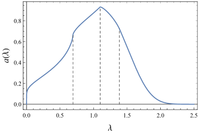
Figure 2: The dimensionless spectral function $a(\lambda)$ in the case of Coulomb interactions, obtained by solving the integral equation (26) numerically. The dashed lines are at $\lambda=\ln 2$, $\ln 3$, and $\ln 4$.

The most striking feature of the spectral functions in Figs. 1 and 2 is the presence of a series of singularities shown by the dashed lines at $\lambda=1-n^{-2}$ and $\lambda=\ln n$, respectively. The features with $n=2$ and $3$ are most prominent, but features with $n$ up to 6 can still be seen in the plots of first and second derivatives of $a(\lambda)$. In both cases these positions correspond to the energies $\epsilon=n\varepsilon(p/n)$ of the states in which the total momentum $p$ is distributed equally among $n$ bosonic excitations. These features can be understood from Eq. (19) using the fact that $A_{p}(\epsilon)=0$ at $\epsilon<\varepsilon(p)$. The latter condition means that the integrand in Eq. (19) vanishes for $\epsilon-\varepsilon(q)<\varepsilon(p-q)$. Since the maximum value of $\varepsilon(q)+\varepsilon(p-q)$ is $2\varepsilon(p/2)$, the integration region effectively changes when $\epsilon$ crosses this value, and the spectral function has a singularity. To understand the feature for $n=3$, one can iterate Eq. (19) to express $A_{p}(\epsilon)$ as a double integral of $A_{p-q-q^{\prime}}(\epsilon-\varepsilon(q)-\varepsilon(q^{\prime}))$ over $q$ and $q^{\prime}$ and repeat the above argument. Successive iterations of Eq. (19) demonstrate the existence of the features at $\epsilon=n\varepsilon(p/n)$ with $n=4,5,\ldots$. Finally, we mention that in both cases of the short-range and Coulomb interactions, the second singularity coincides with the maximum of $a(\lambda)$, i.e., the maximum of $A_{p}(\epsilon)$ is at $\epsilon=3\varepsilon(p/3)$.

Although the exact shape of the spectral function shown in Figs. 1 and 2 was obtained only for the short-range and Coulomb interactions, the above argument does not rely on the specific form of the interaction potential. A similar sequence of singularities is therefore expected for other interactions, including the experimentally relevant case of Coulomb interaction screened by a nearby gate. Experimental observation of these singularities would thus show explicitly the existence of the bosonic excitations and measure their spectrum $\varepsilon(q)$.

To summarize, we have reduced the problem of the evaluation of the spectral function $A_{p}(\epsilon)$ of a system of chiral one-dimensional fermions in the regime of strong interactions to solving the integral equation (19). Although analytical solution of Eq. (19) is not feasible, the numerical solution for a given interaction $V(q)$ is straightforward, see Figs. 1 and 2 for the short-range and Coulomb interactions. The solutions show sharp features at the energies $\epsilon$ at which the momentum of the fermion is transferred to $n$ bosonic excitations with momenta $p/n$ for $n=2,3,4,\ldots$. For the above two types of interactions, the position of the maximum of $A_{p}(\epsilon)$, is determined exactly.

S1 I.  Asymptotic properties of the spectral function in the case of short-range interactions

Here we use the form of the integral equation (22), the normalization condition

$$\int_{0}^{1}a(z)dz=1,$$ (S1)

and the property that $a(\lambda)$ vanishes at $\lambda<0$ and $\lambda>1$ to obtain the behavior of $a(\lambda)$ at the edges of support, $\lambda=0$ and 1.

S1.1 A.  Behavior of $a(\lambda)$ at $\lambda\to 0^{+}$.

Because $a(\lambda)=0$ for negative $\lambda$, at $\lambda<3/4$ the integral in Eq. (22) can be split into two,

$$a(\lambda) = \int_{0}^{\eta}\frac{d\zeta}{\zeta^{3}}a\left(\frac{\lambda-3\zeta(1-\zeta)}{\zeta^{3}}\right)$$ (S2)

$$+\int_{1-\eta}^{1}\frac{d\zeta}{\zeta^{3}}a\left(\frac{\lambda-3\zeta(1-\zeta)}{\zeta^{3}}\right),$$

where

$$\eta(1-\eta)=\frac{\lambda}{3},\quad\eta<\frac{1}{2}.$$

To leading order at $\lambda\to 0$ we have $\eta=\lambda/3$. Since $a(\lambda)\sim 1$, the second term in Eq. (S2) is of the order of $\eta\sim\lambda$. We will see below that this is smaller than the contribution of the first term, i.e., to leading order the behavior of $a(\lambda)$ at $\lambda\to 0$ can be obtained from

$$a(\lambda)=\int_{0}^{\eta}\frac{d\zeta}{\zeta^{3}}a\left(\frac{\lambda-3\zeta(1-\zeta)}{\zeta^{3}}\right).$$

Introducing a new integration variable

$$z=\frac{\lambda-3\zeta(1-\zeta)}{\zeta^{3}},\quad\frac{dz}{d\zeta}=-\frac{3\lambda}{\zeta^{4}}+\frac{6}{\zeta^{3}}-\frac{3}{\zeta^{2}},$$

we obtain

$$a(\lambda)=\int_{0}^{1}\frac{a(z)dz}{\frac{3\lambda}{\zeta}-6+3\zeta}.$$ (S3)

Here we used the fact that $a(\zeta)=0$ at $\zeta>1$ and limited the range of integration accordingly. At this point we notice that at $\lambda\to 0^{+}$ the condition $0<z<1$ requires $\zeta/\lambda\to 1/3$. Substituting this result into Eq. (S3) we find

$$a(0^{+})=\frac{1}{3}\int_{0}^{1}a(z)dz=\frac{1}{3},$$ (S4)

where we used the normalization condition (S1). The numerical solution shown in Fig. 1 is consistent with Eq. (S4).

S1.2 B.  Comparison with the results of Ref. [9]

The behavior of the spectral function at $\epsilon\to\varepsilon(p)$ can be studied using the approach of Ref. [9]. The latter applies to nonchiral systems of fermions and, in addition, it assumes Galilean invariance. To apply their results to our chiral system, one must exclude all effects related to the second (left) Fermi point, which in practice means setting

$$V_{L}=0,\quad\delta_{-}=0,\quad K=1.$$ (S5)

Under these simplifying assumptions, their result is that near the edge of support the spectral function scales as a power of $\epsilon-\varepsilon(p)$ with the exponent

$$\mu=1-\left(\frac{\delta_{+}}{2\pi}\right)^{2}.$$ (S6)

This expression is obtained from Eq. (14) of Ref. [9], where one should choose $\{n,\pm\}\to\{0,-\}$ branch of hole excitations. (The other branches are affected by the second Fermi point.) The phase shift $\delta_{+}$ can be obtained by applying the conditions (S5) to Eqs. (8) and (10) of Ref. [9], which do not rely on Galilean invariance,

$$\delta_{+}=2\pi\frac{\frac{\partial\varepsilon(k)}{\partial k_{F}}+v}{v_{d}-v}.$$ (S7)

Here we have replaced the particle density $\rho$ with $k_{F}/\pi$. In the above expression, $\varepsilon(k)$ is the energy of the hole measured from the Fermi energy which in our case is the energy of the bosonic excitation $\varepsilon(p)$. An important difference is that unlike $k$, our $p$ is measured from the Fermi momentum $k_{F}$. Thus one should substitute into Eq. (S7) the energy $\varepsilon(k)\to\varepsilon(k-k_{F})$. The denominator of Eq. (S7) contains velocity of the hole $v_{d}$, which in our case is simply $\varepsilon^{\prime}(p)=\varepsilon^{\prime}(k-k_{F})$. As a result, in the case of strongly interacting chiral fermions considered in this paper, Eq. (S7) yields $\delta_{+}=-2\pi$.

According to Eq. (S6), this value of $\delta_{+}$ yields power-law scaling of the spectral function with the exponent $\mu=0$ at $\epsilon\to\varepsilon(p)$. This limit corresponds to $\lambda\to 0^{+}$. Thus, our result (S4) also gives $\mu=0$.

S1.3 C.  Behavior of $a(\lambda)$ at $\lambda\to 1^{-}$.

The behavior shown in Fig. 1 suggests that in the limit $\lambda\to 1^{-}$ the dimensionless spectral function $a(\lambda)$ approaches zero exponentially. We will therefore write it in the form

$$a(\lambda)=e^{-\alpha(\chi)},\qquad\chi=1-\lambda$$ (S8)

and study the behavior of $\alpha(\chi)$ at $\chi\to 0^{+}$. We start by defining the function

$$z(\zeta)=\frac{\lambda-3\zeta(1-\zeta)}{\zeta^{3}}=\frac{1-\chi-3\zeta(1-\zeta)}{\zeta^{3}},$$ (S9)

cf. Eq. (22). $z(\zeta)$ has a minimum at $\tilde{\zeta}=1-\sqrt{\chi}$, near which it behaves as

$$z(\zeta)\simeq 1-\tilde{\chi}+3\sqrt{\chi}\,(\zeta-\tilde{\zeta})^{2},\quad\tilde{\chi}=\frac{\chi}{(1-\sqrt{\chi})^{2}}$$ (S10)

where the coefficient of the term $(\zeta-\tilde{\zeta})^{2}$ is written to leading order in $\chi\ll 1$.

We now substitute Eqs. (S8), (S9) and (S10) into Eq. (22),

$$e^{-\alpha(\chi)} \simeq \int_{0}^{1}\frac{d\zeta}{\zeta^{3}}e^{-\alpha(\tilde{\chi}-3\sqrt{\chi}(\zeta-\tilde{\zeta})^{2})}$$

$$\simeq e^{-\alpha(\tilde{\chi})}\int_{0}^{1}\frac{d\zeta}{\zeta^{3}}e^{3\alpha^{\prime}(\tilde{\chi})\sqrt{\chi}(\zeta-\tilde{\zeta})^{2}}$$

We now assume that the derivative $\alpha^{\prime}(\tilde{\chi})$ is negative and sufficiently large to justify applying the saddle point approximation to the above integral. The latter yields

$$e^{\alpha(\tilde{\chi})-\alpha(\chi)}\simeq\sqrt{\frac{\pi}{3|\alpha^{\prime}(\tilde{\chi})|\sqrt{\chi}}}.$$ (S11)

This approximation is applicable provided that $|\zeta-\tilde{\zeta}|\sim 1/\sqrt{|\alpha^{\prime}|\sqrt{\chi}}\ll 1-\tilde{\zeta}=\sqrt{\chi}$, i.e.,

$$\chi^{3/2}|\alpha^{\prime}(\tilde{\chi})|\gg 1,$$ (S12)

which will be verified later. To leading order one can expand the exponent in the left-hand side of Eq. (S11) and obtain

$$|\alpha^{\prime}(\tilde{\chi})|(\chi-\tilde{\chi})=\frac{1}{2}\ln\frac{\pi}{3|\alpha^{\prime}(\tilde{\chi})|\sqrt{\chi}}$$

or, substituting $\tilde{\chi}\simeq\chi+2\chi^{3/2}$ from Eq. (S10),

$$4\chi^{3/2}|\alpha^{\prime}(\tilde{\chi})|=\ln\frac{3|\alpha^{\prime}(\tilde{\chi})|\sqrt{\chi}}{\pi}.$$ (S13)

We now present $|\alpha^{\prime}(\tilde{\chi})|$ as

$$|\alpha^{\prime}(\tilde{\chi})|=\frac{\xi}{4\chi^{3/2}}.$$ (S14)

Equation (S13) then takes the form

$$\xi=\ln\frac{3\xi}{4\pi\chi}.$$ (S15)

To leading order at $\chi\to 0^{+}$, we find

$$\xi\simeq\ln\frac{3}{4\pi\chi}.$$ (S16)

Note that this guarantees $\xi\gg 1$, i.e., the condition (S12) for the applicability of the saddle point approximation (S11) is satisfied. Using Eqs. (S14) and (S16) and keeping in mind that $\alpha^{\prime}<0$, we obtain

$$\alpha(\chi)\simeq\frac{1}{2\sqrt{\chi}}\left(\ln\frac{3}{4\pi\chi}-2\right).$$ (S17)

The error in the approximate solution (S16) of Eq. (S15) is of the order of $\ln(\ln(1/\chi))$. Thus the coefficient in the argument of the logarithm in Eq. (S17) must be omitted. This yields

$$\alpha(\chi)\simeq\frac{1}{2\sqrt{\chi}}\ln\frac{1}{\chi},$$ (S18)

which is equivalent to Eq. (23) of the main text.

S2 2.  Asymptotic properties of the spectral function in the case of Coulomb interactions

Here we study the asymptotic properties of the solution of the integral equation (26) at $\lambda\to 0^{+}$ and $\lambda\to\infty$. For convenience, we rewrite Eq. (26) as

$$a(\lambda)=\int_{0}^{1}\frac{d\zeta}{\zeta}a\left(\frac{\lambda-f(\zeta)}{\zeta}\right),$$ (S19)

where

$$f(\zeta)=\zeta\ln\frac{1}{\zeta}+(1-\zeta)\ln\frac{1}{1-\zeta}.$$ (S20)

We are interested in the solution that satisfies the normalization condition

$$\int_{0}^{\infty}a(z)dz=1$$ (S21)

and vanishes at $\lambda<0$.

S2.1 A.  Behavior of $a(\lambda)$ at $\lambda\to 0^{+}$

Because $a(\lambda)=0$ at negative $\lambda$, under the conditions $0<\lambda<{\rm max}f(\zeta)=\ln 2$ one can rewrite Eq. (S19) as

$$a(\lambda)=\int_{0}^{\eta}\frac{d\zeta}{\zeta}a\left(\frac{\lambda-f(\zeta)}{\zeta}\right)+\int_{1-\eta}^{1}\frac{d\zeta}{\zeta}a\left(\frac{\lambda-f(\zeta)}{\zeta}\right),$$

where $\eta$ is defined by

$$f(\eta)=\lambda,\quad 0<\eta<\frac{1}{2}.$$ (S22)

We are interested in the regime $\lambda\ll 1$, which corresponds to $\eta\ll 1$. In this case the second integral, in which $\zeta$ is close to 1, is much smaller than the first one, where $\zeta\leq\eta$. Omitting it and replacing $\zeta=(1-u)\eta$, we obtain

$$a(\lambda)=\int_{0}^{1}\frac{du}{1-u}a\left(\frac{f(\eta)-f((1-u)\eta)}{(1-u)\eta}\right).$$ (S23)

At small $\zeta$ one can approximate

$$f(\zeta)\simeq\zeta\ln\frac{1}{\zeta}$$ (S24)

and obtain

$$f(\eta)-f((1-u)\eta)\simeq u\eta\ln\frac{1}{\eta}-\eta(1-u)\ln\frac{1}{1-u}\simeq u\eta\ln\frac{1}{\eta}.$$

The argument of the function $a(\lambda)$ in the integrand of Eq. (S23) is then

$$\frac{f(\eta)-f((1-u)\eta)}{(1-u)\eta}\simeq\frac{u\ln\frac{1}{\eta}}{1-u}.$$

Since $a(\lambda)$ falls off rapidly at $\lambda\gg 1$, the integral (S23) is dominated by the values of $u\sim 1/\ln\frac{1}{\eta}\ll 1$. This enables us to approximate $1-u\simeq 1$ and to extend the integration over $u$ to infinity,

$$a(\lambda)\simeq\int_{0}^{\infty}du\,a\left(u\ln\frac{1}{\eta}\right).$$ (S25)

Using the normalization condition (S21), we obtain

$$a(\lambda)\simeq\frac{1}{\ln\frac{1}{\eta}},$$ (S26)

where $\eta$ should be obtained by solving the equation

$$\eta\ln\frac{1}{\eta}=\lambda,$$ (S27)

obtained from Eqs. (S22) and (S24). Taking the logarithm of both sides of Eq. (S27), we obtain

$$\ln\frac{1}{\eta}-\ln\left(\ln\frac{1}{\eta}\right)=\ln\frac{1}{\lambda},$$ (S28)

At very small $\eta$ one can neglect the second term in the left-hand side of Eq. (S28) and obtain

$$a(\lambda)\simeq\frac{1}{\ln\frac{1}{\lambda}},$$ (S29)

cf. Eq. (27) of the main text. A more accurate result

$$a(\lambda)\simeq\frac{1}{\ln\frac{1}{\lambda}+\ln\big{(}\ln\frac{1}{\lambda}\big{)}}.$$ (S30)

is obtained by iterating Eq. (S28) once.

S2.2 B.  Behavior of $a(\lambda)$ at $\lambda\to\infty$

Figure 2 suggests that at $\lambda\to\infty$ the spectral function falls off exponentially. We thus present it in the form

$$a(\lambda)=e^{-\beta(\lambda)}$$ (S31)

where the function $\beta(\lambda)$ is expected to approach infinity at large $\lambda$. We now examine the integral equation (S19) to obtain asymptotic behavior of $\beta(\lambda)$ at $\lambda\to\infty$.

To this end we introduce the function

$$\Lambda(\zeta)=\frac{\lambda-f(\zeta)}{\zeta}.$$ (S32)

The latter has a minimum at $\tilde{\zeta}=1-e^{-\lambda}$, near which it behaves as

$$\Lambda(\zeta)\simeq\tilde{\lambda}+\frac{e^{\lambda}}{2\tilde{\zeta}^{2}}(\zeta-\tilde{\zeta})^{2},\qquad\tilde{\lambda}=\lambda+\ln(1-e^{-\lambda}).$$ (S33)

Assuming that not only $\beta(\lambda)$, but also its derivative is large at $\lambda\to\infty$, the integral in Eq. (S19) can be evaluated using the saddle point approximation:

$$e^{-\beta(\lambda)} \simeq e^{-\beta(\tilde{\lambda})}\int_{0}^{1}\frac{d\zeta}{\zeta}e^{-\beta^{\prime}(\tilde{\lambda})\frac{e^{\lambda}}{2\tilde{\zeta}^{2}}(\zeta-\tilde{\zeta})^{2}}$$ (S34)

$$\simeq e^{-\beta(\tilde{\lambda})}\sqrt{\frac{2\pi}{\beta^{\prime}(\tilde{\lambda})e^{\lambda}}}.$$

The condition of applicability of the saddle point approximation is that the typical $|\zeta-\tilde{\zeta}|$ in the integral is small compared to $1-\tilde{\zeta}$, i.e.,

$$\frac{1}{\sqrt{\beta^{\prime}(\tilde{\lambda})e^{\lambda}}}\ll e^{-\lambda},$$

is satisfied for our result (S36). Rewriting Eq. (S34) as

$$e^{\beta(\tilde{\lambda})-\beta(\lambda)}\simeq\sqrt{\frac{2\pi}{\beta^{\prime}(\tilde{\lambda})e^{-\lambda}}}\,e^{-\lambda}$$

and expanding $\beta(\tilde{\lambda})-\beta(\lambda)\simeq\beta^{\prime}(\tilde{\lambda})(\tilde{\lambda}-\lambda)$ we obtain

$$\beta^{\prime}(\tilde{\lambda})e^{-\lambda}\simeq\lambda+\frac{1}{2}\ln\frac{\beta^{\prime}(\tilde{\lambda})e^{-\lambda}}{2\pi}.$$ (S35)

To leading order at $\lambda\to\infty$ one can replace $\tilde{\lambda}\to\lambda$ and neglect the second term on the right-hand side. This yields

$$\beta^{\prime}(\lambda)\simeq\lambda e^{\lambda}$$ (S36)

and thus

$$\beta(\lambda)\simeq\lambda e^{\lambda}.$$ (S37)

Note that we have replaced $(\lambda-1)\to\lambda$ in the prefactor, because the leading order correction in Eq. (S36) is $\frac{1}{2}(\ln\lambda)e^{\lambda}\gg e^{\lambda}$. Equation (S37) is equivalent to $\ln a(\lambda)\simeq-\lambda e^{\lambda}$, as quoted in the main text.