A global bifurcation organizing rhythmic activity in a coupled network

Abstract

We study a system of coupled phase oscillators near a saddle-node on an invariant circle bifurcation and driven by random intrinsic frequencies. Under the variation of control parameters, the system undergoes a phase transition changing the qualitative properties of collective dynamics. Using the Ott-Antonsen reduction and geometric techniques for ordinary differential equations, we identify a heteroclinic bifurcation in a family of vector fields on a cylinder, which explains the change in collective dynamics. Specifically, we show that the heteroclinic bifurcation separates two topologically distinct families of limit cycles: contractible limit cycles before the bifurcation from noncontractibile ones after the bifurcation. Both families are stable for the model at hand.

The Kuramoto model (KM) of coupled phase oscillators provides an important paradigm for studying collective dynamics in systems ranging from neuronal networks to swarms of fireflies to power grids. The classical KM features a remarkable phase transition separating stable mixing dynamics from gradual build-up of synchronization. During the latter phase, the oscillators form a cluster whose coherence (measured by the order parameter) remains approximately constant and increases with the coupling strength. If the uniformly rotating phase oscillators in the KM are replaced by those close a saddle-node on invariant circle bifurcation, the order parameter does not stay constant anymore. Instead, it undergoes slow-fast oscillations. Furthermore, for larger values of the coupling strength the system undergoes a phase transition, which changes the character of oscillations qualitatively. Previous studies based in part on numerical bifurcation techniques revealed a rich bifurcation structure of the modified KM. In this paper, we use the Ott-Antonsen reduction and qualitative methods for ordinary differential equations to study collective dynamics in the modified model with an emphasis on the slow-fast oscillations of the order parameter. We analytically locate the Andronov-Hopf and Bogdanov-Takens bifurcations for the system of equations governing the order parameter and identify the relevant normal form for the Bogdanov-Takens bifurcations. Furthermore, we relate the phase transition in the modified model to a nonlocal bifurcation in one parameter families of vector fields on a cylinder. The results of this work show that the slow-fast oscillations of the order parameter in the modified KM are shaped by the proximity to both Bogdanov-Takens and heteroclinic bifurcations.

1 Introduction

The KM plays a special role in the theory synchronization. It provides a framework for studying synchronization and other forms of collective dynamics in systems of coupled oscillators with random parameters. Despite its analytical simplicity, studies of the KM revealed and helped to understand some very nontrivial phenomena in collective dynamics, which are relevant to a range of models in physics and biology (e.g., the onset of synchronization and chimera states [23, 22, 38]). Motivated by models featuring type I excitability in mathematical biology, we modify the KM by placing the individual oscillators close a saddle node on an invariant circle bifurcation. Specifically, we consider the following coupled system

$$\dot{\theta}_{i}=1+\omega_{i}-\cos\theta_{i}+Kn^{-1}\sum_{j=1}^{n}\sin\left(\theta_{j}-\theta_{i}\right),\quad i\in[n]:=\{1,2,\dots,n\},$$ (1.1)

where $\theta_{i}:{\mathbb{R}}^{+}\to\operatorname{\mathbb{T}}:={\mathbb{R}}/2\pi{\mathbb{R}}$ is the state of oscillator $i$ at time $t$ and $K\geq 0$ is the coupling strength. Parameter $\omega_{i}$ controls the frequency of oscillator $i$, if $\omega_{i}>0$, or defines the excitation threshold otherwise. We assume that $\omega_{i}$’s are sampled from a unimodal probability distribution with density $g(\omega)$. Equation (1.1) fits into the framework of the coupled active rotators model considered by Shinomoto and Kuramoto in [37]. In contrast to our setting, they used identical oscillators (i.e., $\omega_{i}=\operatorname{const}$) albeit forced by small noise. Different variants of the active rotators model with and without noise were studied more recently by other authors [1, 42, 44, 20, 21]. We comment on the relation of our findings to the results in these papers below.

To take a full advantage of the Ott-Antonsen Ansatz [33] below, we restrict to the Lorentzian distribution with density

$$g(\omega)=\frac{\delta}{\pi\left(\omega-\epsilon^{2}\right)^{2}+\delta^{2}},$$ (1.2)

where $\epsilon^{2}$ and $\delta>0$ are the location and scale parameters respectively. Lorentzian distribution is commonly used in the studies of the collective dynamics in the Kuramoto model and related systems, because it fits nicely into the Ott-Antonsen Ansatz (see, e.g., [34, 32]). There has been a concern that due to its special properties (lack of finite moments) models based on Lorentzian distribution may feature nongeneric scenarios [26]. We checked that in qualitative form the bifurcation scenarios reported in this paper hold for Gaussian distribution, and, thus, are relevant to a large class of models based on unimodal probability distributions. If typical realizations of $\omega_{i}$ are $O(1)$ and positive then the dynamics of (1.1) is practically the same as in the classical KM. Specifically, for small $K$ the oscillators are highly incoherent. Starting with a certain critical value of $K$, the coherence gradually increases [38]. Thus, in this paper, we focus on the regime when typical values of $\omega_{i}^{\prime}s$ are small, i.e., when the individual oscillators are close a saddle-node bifurcation.

To describe the collective dynamics of (1.1) we need to remind the reader the definition of the Kuramoto’s order parameter:

$$h_{n}=n^{-1}\sum_{j=1}^{n}e^{\mathrm{i}\mkern 1.0mu\theta_{j}},\quad h_{n}=\rho_{n}e^{\mathrm{i}\mkern 1.0mu\phi_{n}}.$$ (1.3)

The modulus, $\rho_{n}=|h_{n}|$, and the argument, $\phi_{n}=\operatorname{arg}h_{n}$, of the complex order parameter yield the degree of coherence and the position of the center of mass of the population of oscillators on the unit circle respectively. The combination of these two quantitates as functions of time provides a good description of the collective dynamics. In the classical Kuramoto, after some transients the modulus of the order parameter approaches a steady value (up to $O(n^{-1/2})$ fluctuations) while the argument drifts with approximately constant velocity. In contrast, in the simulations of the modified KM (1.1) we observe very nonuniform slow-fast oscillations in the modulus and the argument of the complex order parameter (Figure 1).

We now turn to describe the salient features of the collective dynamics of (1.1). There are three main regimes in the system dynamics:

I

For small values of $K$, the individual oscillators rotate in the counterclockwise direction but the overall distribution of oscillators on a unit circle remains practically stationary. The distribution has a peak at $\theta=0$ reflecting the fact that the oscillators slow down in a neighborhood of $\theta=0$ and thus spend more time there (see Figure 2a). The order parameter lies on the real axis very close to $1$ and stays approximately constant (see inset in Figure 2a).

II

There are two critical values of $K$: $0<K_{AH}<K_{HC}$, which will be shown below to correspond to an Andronov-Hopf bifurcation and a heteroclinic bifurcation respectively. For $K\in(K_{AH},K_{HC})$ the order parameter undergoes slow-fast oscillations (see Figure 1). Importantly, the argument of the order parameter stays between $\frac{-\pi}{2}$ and $\frac{\pi}{2}$ (see the insets in Figures 2b,c). This means that the center of mass of the population of oscillators oscillates around $\theta=0$. The modulus of the order parameter varies between values close to $0$ and $1$ spending more time in the region near $1$ (Figure 1). Two snapshots of the distribution of the oscillators on a unit circle are shown in Figure 2b (coherent phase) and Figure 2c (incoherent phase).

III

Two representative episodes of the system dynamics for larger values of $K$ are shown in Figure 2d and e. As before, the oscillators slow down and accumulate as they approach the origin and accelerate and spread around once they have passed it. However, there is an important distinction from the previous regime. It is quite pronounced in numerical simulations and can also be seen from the static snapshots in Figure 2. Recall that for small values of $K$ ($K<K_{HC}$) the order parameter never leaves the right half plane. For larger $K$ ($K>K_{HC}$), on the other hand, the order parameter makes a full revolution around the origin in one cycle of oscillations (see the insets in Figure 2 d,e). The change in the qualitative character of oscillations can be seen from the timeseries of $\phi_{n}$ for two different values of $K$ in Figure 1 b. Note that for small $K$, $\phi_{n}$ undergoes small oscillations, while for large values of $K$, the range of $\phi_{n}$ covers the entire circle. One can compare this to small oscillations versus full swing revolutions of the pendulum. Below, we show that indeed the two regimes are qualitatively (topologically) distinct and are separated by a bifurcation.

In contrast to the classical scenario of transition to synchronization in the original KM, where one observes the formation of a single coherent cluster drifting uniformly around the unit circle [23, 38], in the modified model (1.1), we see pronounced oscillations in the argument of the order parameter (Figure 2 b-e). The amplitude of these oscillations increases until the oscillations are transformed into a rotational motion of the center of mass of the population of the oscillators around the unit circle (Figure 2 d,e). Another salient feature of this transtion is the slow-fast character of the oscillations of the order parameter (Figure 1).

Periodic regimes in macroscopic dynamics in the model of active rotators were described already in [37]. These regimes were found by numerical simulations. Pulsating oscillations of the order parameter similar to those shown in Figure 1 were reported in the subsequent studies of the coupled active rotators with and without noise [20, 42, 44]. In [20, 42], the authors derived a system of differential equations for the modulus $\rho$ and the argument $\phi$ of the order parameter (1.3) in the limit as $n\to\infty$. Using the combination of self-consistent analysis and numerical bifurcation techniques, both studies revealed an Andronov-Hopf, Bogdanov-Takens, and homoclinic bifurcations in the parameter regime relevant to transition to synchronization. Similar results were obtained for a coupled system of noisy rotators in [44] albeit via a different approximation procedure. Previous studies reveal a rich bifurcation structure underlying macroscopic dynamics in the coupled model. In this paper, we focus on the origins of the slow-fast oscillations of the order parameters and, in particular, on the transition from the oscillatory to rotational motion of the order parameter. We use the qualitative methods for ordinary differential equations to elucidate the bifurcation structure of the coupled model. Specifically, we locate the Andronov-Hopf and Bogdanov-Takens bifurcations analitically and identify the relavant normal form for the Bogdanov-Takens bifurcation. Furthermore, we relate the transition to the rotational motion to a heteroclinic bifurcation of a family of vector fields on a cylinder. A related global bifurcation separating oscillations from rotations of the order parameter in the model of noisy active rotators was reported (but not analyzed) in [44]. In Section 4, we provide a detailed analysis of the heteroclinic bifurcation for the model at hand.

There is an extensive literature on the KM. Early papers were devoted mostly to synchronization (cf. [23, 39, 40, 38]). The scope of more recent contributions encompasses rigorous mathematical aspects of synchronization [6, 10, 7], complex spatiotemporal patterns [35, 31], generalizations or adaptations of the classical KM [8, 9, 27], as well as applications to physical and biochemical systems (see, e.g., [36, 30, 12]). Our work is close in spirit to [9, 43] where the modifications of the KM were used to tackle challenging questions about collective dynamics. Specifically, we wanted to understand collective dynamics in populations of type I excitable oscillators with randomly distributed intrinsic frequencies. Coupled networks of this type have been studied in computational neuroscience (see, e.g., [15, 14, 29]) albeit in settings that differ from that adopted here. In particular, methods for studying weakly coupled networks (cf. [17]) do not apply to systems with random parameters like (1.1). For coupled systems with different coupling type, collective dynamics in closely related models of coupled theta neurons was analyzed in [28, 19, 32]. We believe that the analysis of the modified KM used in this paper complements the previous studies of coupled active rotators in [20, 42, 44] and brings new insights to understanding collective dynamics of type I oscillators.

a b

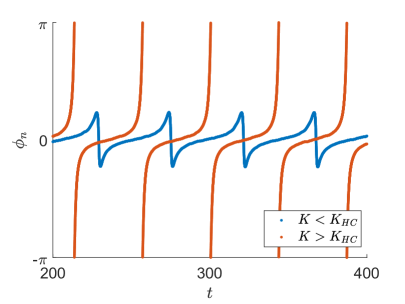
Figure 1: The time series of the modulus, $\rho_{n}$, and the argument, $\phi_{n}$, of the complex order parameter plotted for $K=0.23$ (blue) and $K=0.4$ (orange) with $n=2000$. Note that in b the oscillations of $|\phi_{n}|$ do not exceed $\pi/2$ for small $K$, whereas the oscillations of $\phi_{n}$ cover the entire range for $K$ sufficiently large. Intrinsic frequencies are sampled from the Lorentzian distribution (1.2) with $\epsilon=0.1$, $\delta=0.01$.

The paper is organized as follows. In the next section, we use the Ott-Antonsen Ansatz [33] to derive a system of two ordinary differential equations, which captures the long time dynamics of the coupled system. In Section 3, we analyze the reduced system. The analysis uses the unfolding of the Bogdanov-Takens bifurcation among other qualitative techniques for ordinary differential equations. Further, we identify a heteroclinic bifurcation, which explains the phase transition in the collective dynamics. The heteroclinic bifurcation is analyzed in Section 4. In Section 5, we relate the analysis of the reduced system to the collective dynamics of (1.1). We conclude with a brief discussion of the main results in Section 6.

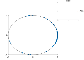
a  b 

c 

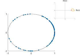
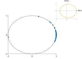
d  e 

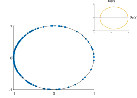
Figure 2: Plots in each row illustrate three distinct regimes in collective dynamics for three values of $K$: ($K=0.05$ in a), ($K=0.17$ in b,c) and ($K=0.4$ in d,e). The values of other parameters are $\delta=0.01$, $\epsilon=0.1$, and $n=2000$ (though for ease of visualization we plot a random sampling of $200$ oscillators). Snapshot a shows the equilibrium distribution (though we emphasize that individual oscillators travel around the circle). The snapshots in b, c show the location of the oscillators in phase space at two moments of time during one period of oscillations. Note that the coherence varies from high in b to low in c. The variation in coherence is also observed in the snapshots made for larger value of $K$ shown in d,e. However, in the former case the oscillations of the center of mass of the population are restricted to the left half-plane, whereas in the latter case the center of mass travels around the circle. This can be seen from the trajectories of the complex order parameter shown in the insets. Note that the orbit traced by the order parameter in d, e encircles the origin. In contrast, in b, c the argument of the order parameter remains between $(-\pi/2,\pi/2)$ for all times.

2 The mean field limit

In the large $n$ limit, the dynamics of (1.1) is described by the following Vlasov equation (cf. [11, 39])

$$\partial_{t}f(t,\theta,\omega)+\partial_{\theta}\left\{V(t,\theta,\omega)f(t,\theta,\omega)\right\}=0,$$ (2.1)

where $f(t,\theta,\omega)d\theta d\omega$ is the probability of $(\theta,\omega)\in(\theta,\theta+d\theta)\times(\omega,\omega+d\omega)$ at time $t\in{\mathbb{R}}^{+}$. The velocity field is defined by

$$V(t,\theta,\omega)=1+\omega-\frac{e^{\mathrm{i}\mkern 1.0mu\theta}+e^{-\mathrm{i}\mkern 1.0mu\theta}}{2}+{K\over 2\mathrm{i}\mkern 1.0mu}\left(h(t)e^{-\mathrm{i}\mkern 1.0mu\theta}-\overline{h(t)e^{-\mathrm{i}\mkern 1.0mu\theta}}\right),$$ (2.2)

where

$$h(t):=h[f(t,\cdot)]=\int_{\operatorname{\mathbb{T}}\times{\mathbb{R}}}e^{\mathrm{i}\mkern 1.0mu\theta}f(t,\theta,\omega)d\theta d\omega,$$ (2.3)

is the continuum order parameter.

From (1.1) with $K=0$ one can determine the stationary distribution of the oscillators in the phase space:

$$f_{st}(\theta,\omega)=\frac{j(\omega)}{1+\omega-\cos\theta},$$

where $j(\omega)$ is subject to the following equation

$$j(\omega)\int_{\operatorname{\mathbb{T}}}\frac{d\theta}{1+\omega-\cos\theta}=g(\omega).$$

To investigate (2.1) for $K\geq 0$, we invoke the Ott-Antonsen Ansatz [33]

$$f(t,\theta,\omega)=\frac{g(\omega)}{2\pi}\left\{1+\sum_{k=1}^{\infty}\left[\alpha(t,\omega)^{k}e^{\mathrm{i}\mkern 1.0muk\theta}+\overline{\alpha(t,\omega)}^{k}e^{-\mathrm{i}\mkern 1.0muk\theta}\right]\right\}.$$ (2.4)

Previous studies of the KM suggest that the Ott-Antonsen Ansatz correctly describes the long time asymptotic behavior of solutions of this model. It has been used to study chimera states [31] among many other spatiotemporal patterns in the KM and related models [34, 27, 20, 42, 32]. There is a convincing albeit not completely rigorous mathematical argument justifying the use of this Ansatz for studying the long time behavior of solutions of the Kuramoto model. The analysis in the remainder of this paper relies on the validity of the Ott-Antonsen Ansatz.

By plugging (2.4) into (2.1), we obtain

$$\partial_{t}\alpha=\frac{K}{2}\left(\bar{h}-h\alpha^{2}\right)+\mathrm{i}\mkern 1.0mu\left(\frac{1}{2}-\alpha\omega+\frac{\alpha^{2}}{2}\right).$$ (2.5)

Multiplying both sides by $2$ and rescaling time in (2.5) yields

$$\partial_{t}\alpha=K\left(\bar{h}-h\alpha^{2}\right)+\mathrm{i}\mkern 1.0mu\left(1-2\alpha\omega+\alpha^{2}\right).$$ (2.6)

Equation (2.6) is simpler than the Vlasov equation (2.1), but it is still an integro-partial differential equation. For the Lorentzian density $g(\omega)$ given in (1.2), one can further reduce (2.6) to the following ordinary differential equation (cf. [33])

$$\alpha^{\prime}=-2\alpha\delta+K\left(\alpha-\alpha|\alpha|^{2}\right)+\mathrm{i}\mkern 1.0mu\left(1-2\alpha\left(1+\epsilon^{2}\right)+\alpha^{2}\right),$$ (2.7)

where by abuse of notation we continue to denote $\alpha(t,\epsilon^{2}-\mathrm{i}\mkern 1.0mu\delta)$ by $\alpha(t)$. Furthermore, the order parameter $h$ can now be expressed through $\alpha$:

$$h(t)=\overline{\alpha(t)}.$$ (2.8)

Equation (2.7) can be written as an ordinary differential equation on ${\mathbb{R}}^{2}$:

$$\begin{pmatrix}x^{\prime}\\ y^{\prime}\end{pmatrix}=\begin{pmatrix}0\\ 1\end{pmatrix}+\begin{pmatrix}K-2\delta&2(1+\epsilon^{2})\\ -2(1+\epsilon)&K-2\delta\end{pmatrix}\begin{pmatrix}x\\ y\end{pmatrix}+(x^{2}+y^{2})\begin{pmatrix}x\\ -1-y\end{pmatrix},$$ (2.9)

where $\alpha=x+\mathrm{i}\mkern 1.0muy$. Since we are interested in the macroscopic dynamics of (1.1), we want to track the changes the qualitative behavior of the modulus and the argument of the order parameter. To this end, we rewrite (2.7) in polar coordinates $\alpha=\rho e^{\mathrm{i}\mkern 1.0mu\phi}$:

$$\begin{split}\rho^{\prime}&=\left(1-\rho^{2}\right)\left(\sin\phi+K\rho\right)-2\delta\rho,\\ \phi^{\prime}&=\rho^{-1}\left(1+\rho^{2}\right)\cos\phi-2\left(1+\epsilon^{2}\right).\end{split}$$ (2.10)

The polar coordinate transformation blows up the origin in the $x-y$ plane to a $\rho=0$ circle. This singular change preserves a $1-1$ correspondence between the trajectories of (2.9) and (2.10) lying in ${\mathbb{R}}^{2}/\{0\}$ and $R^{+}\times\operatorname{\mathbb{T}}$ respectively (cf. [4, §2.8]). The two systems are topologically equivalent in these domains. The right-hand side of (2.10) has a singularity at $\rho=0$. To resolve this singularity, we multiply both sides of the equations in (2.10) by $\rho$ and rescale time to obtain

$$\begin{split}\dot{\rho}&=\rho\left(1-\rho^{2}\right)\left(\sin\phi+K\rho\right)-2\delta\rho^{2},\\ \dot{\phi}&=\left(1+\rho^{2}\right)\cos\phi-2\left(1+\epsilon^{2}\right)\rho.\end{split}$$ (2.11)

Systems (2.10) and (2.11) are topologically equivalent on ${\mathbb{R}}^{+}\times\operatorname{\mathbb{T}}$. However, the latter defines a smooth vector field over ${\mathbb{R}}\times\operatorname{\mathbb{T}}$. It can be studied by standard methods of the qualitative theory for differential equations. In particular, this allows us to resolve the singularity of (2.10) at $\rho=0$, which is important for understanding the macroscopic dynamics of the coupled system.

3 Qualitative analysis of the planar system

In this section, we analyze (2.11) when $K,\delta,\epsilon$ are nonnegative and small.

There are two fixed points of (2.11):

$$\left(0,\frac{\pi}{2}\right),\left(0,\frac{-\pi}{2}\right).$$ (3.1)

Additionally, when $\delta=\epsilon=0$ we can explicitly calculate a third fixed point at $(1,0)$. We begin with the local analysis around $\left(1,0\right)$. This is followed by the linearization about the other two fixed points. After that we combine this information and identify a nonlocal bifurcation of the vector field responsible for the transformation of the collective dynamics in (1.1).

3.1 The Bogdanov-Takens singularity

Let $\rho=1-r$ and rewrite (2.11) in the neighborhood of $(1,0)$ keeping terms up to and including order $2$ to obtain

$$\begin{split}\dot{r}&=-2r\phi-2rK+2\delta+O(3),\\ \dot{\phi}&=-\phi^{2}+r^{2}-2\epsilon^{2}+O(3).\end{split}$$ (3.2)

With $\epsilon=\delta=K=0$ (3.2) fits into the normal form of the Bogdanov-Takens bifurcation [2, 5, 41]:

$$\begin{split}\dot{r}&=-2r\phi,\\ \dot{\phi}&=-\phi^{2}+r^{2}.\end{split}$$ (3.3)

Rewriting (3.3) in polar coordinates $r=a\cos\psi,\;\phi=a\sin\psi$, we obtain

$$\begin{split}\dot{a}&=-a^{2}\sin\psi,\\ \dot{\psi}&=a\cos\psi.\end{split}$$ (3.4)

From (3.4) one can plot the phase portrait of (3.3) (see Figure 3a).

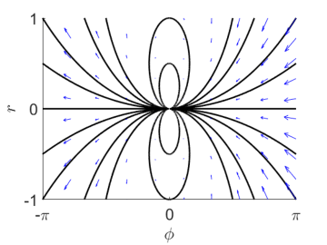
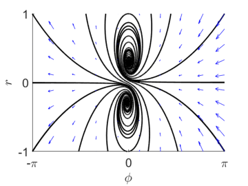
a   b 
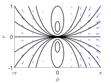
c   d 

Figure 3: Phase portraits for (3.2). a) For $K=\delta=\epsilon=0$, the system is at the Bogdanov-Takens bifurcation. b) Upon increasing $\epsilon$, it becomes an integrable system with two centers (see (3.5); $K=\delta=0$, $\epsilon=0.2$). c) Further, increasing $K$ and $\delta$ transforms the two centers into foci ($K=\delta=0.01$, $\epsilon=0.2$). d) For larger $K$, the system undergoes an Andronov-Hopf bifurcation, which gives birth to a stable limit cycle ($K=0.09$, $\delta=0.01$, $\epsilon=0.2$).

Next, we keep $\delta=K=0$ and let $0<\epsilon\ll 1$. By increasing $\epsilon$ from $0$, we observe that the fixed point at the origin bifurcates into two fixed points: $(0,\sqrt{2}\epsilon)$ and $(0,-\sqrt{2}\epsilon)$. Furthermore, the system has an integral (cf. [16])

$$J(r,\phi)=\frac{r^{2}+\phi^{2}+\epsilon^{2}}{r}.$$ (3.5)

Thus, the trajectories are given by two families of circles:

$$(r-c)^{2}+\phi^{2}=c^{2}-\epsilon^{2}$$

for $c\geq\epsilon$ and $c\leq-\epsilon$. As $c^{2}\to\infty$ they limit onto $r$-axis (Fig. 3b).

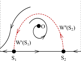
a  b  c 

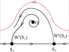
Figure 4: Schematic phase portraits just before, at, and right after the heteroclinic bifurcation. The periodic orbits in a and c (plotted in red) bifurcate from the heteroclinic loops shown in b. Here and below, the phase portraits are identified along lateral sides (see dashed lines).

Next suppose $\epsilon,\delta,$ and $K$ are positive and small. To study this case we use the following scaling:

$$\delta=\nu\epsilon,K=\mu\epsilon,r:=\epsilon\tilde{r},\phi=\epsilon\tilde{\phi}.$$ (3.6)

By plugging (3.6) into (3.2), we have

$$\begin{split}\epsilon^{-1}\dot{\tilde{r}}&=-2\tilde{r}\tilde{\phi}-2\mu\tilde{r}+2\nu,\\ \epsilon^{-1}\dot{\tilde{\phi}}&=-\tilde{\phi}^{2}+\tilde{r}^{2}-1.\end{split}$$ (3.7)

Treating $\nu$ and $\mu$ as positive and small parameters of the same order, we locate the fixed point of (3.7) $(\bar{r},\bar{\phi})$ with positive $\bar{r}$:

$$\bar{\phi}\approx\nu-\mu,\bar{r}\approx 1.$$

Linearization about $(\bar{r},\bar{\phi})$ yields:

$$\epsilon^{-1}\dot{\xi}=A\xi,\quad A=-2\begin{pmatrix}\bar{\phi}+\mu&\bar{r}\\ -\bar{r}&\bar{\phi}\end{pmatrix}.$$

Note

$$\operatorname{Tr}A=-4\nu+2\mu,\quad\det A=4\left(\bar{\phi}^{2}+\bar{r}^{2}+\bar{\phi}\mu\right).$$

The determinant of $A$ is positive for sufficiently small $\mu\geq 0$ (recall that $\bar{r}=O(1)$). For $0\leq\mu<2\nu$ the fixed point $(\bar{r},\bar{\phi})$ is a stable focus. It becomes unstable for $\mu>2\nu$. At $\mu=2\nu$ the system undergoes a supercritical Andronov-Hopf bifurcation (see Figure 3d).

3.2 The heteroclinic bifurcation

We now turn to the remaining two fixed points: $S_{1}=(0,-\pi/2)$ and $S_{2}=(0,\pi/2)$. Linearization about $S_{1}$ yields

$$\begin{pmatrix}\dot{\xi}\\ \dot{\eta}\end{pmatrix}=\begin{pmatrix}-1&0\\ -2(1+\epsilon^{2})&1\end{pmatrix}\begin{pmatrix}\xi\\ \eta\end{pmatrix}+\begin{pmatrix}(K-2\delta)\xi^{2}+O(3)\\ O(3)\end{pmatrix}.$$

The eigenvalues are $\lambda_{1}=1$ and $\lambda_{2}=-1$ with the corresponding eigenvectors $v_{1}=(1,0)$ and $v_{2}=(1,1+\epsilon^{2})$.

Similarly, linearization about $S_{2}$ yields

$$\begin{pmatrix}\dot{\xi}\\ \dot{\eta}\end{pmatrix}=\begin{pmatrix}1&0\\ -2(1+\epsilon^{2})&-1\end{pmatrix}\begin{pmatrix}\xi\\ \eta\end{pmatrix}+\begin{pmatrix}(K-2\delta)\xi^{2}+O(3)\\ O(3)\end{pmatrix}.$$

The eigenvalues are $\lambda_{1}=1$ and $\lambda_{2}=-1$ with the corresponding eigenvectors $v_{1}=(1,-1-\epsilon^{2})$ and $v_{2}=(1,0)$. Consider $D=[-1,1]\times\operatorname{\mathbb{T}}$. In the parameter regime of interest, $D$ is positively invariant. Denote the branches of stable and unstable manifolds of $S_{1}$ and $S_{2}$ lying in $D$ by $W^{s}(S_{1,2})$ and $W^{u}(S_{1,2})$ respectively.

In the remainder of this section, we assume that $0<\epsilon\ll 1$ is fixed. Both $K$ and $\delta$ are also nonnegative and $O(\epsilon)$. Further, we fix $\delta$ and treat $K$ as a control parameter. The linearization about $S_{1}$ and $S_{2}$ shows that both are saddles. The unstable manifold of $S_{1}$ and the stable manifold of $S_{2}$ lie in $\{\rho=0\}$ (Fig. 4). The unstable manifold of $S_{2}$ and the stable manifold of $S_{1}$ are tangent to $(1,-1-\epsilon^{2})$ and $(1,1+\epsilon^{2})$ respectively. Recall that there is another fixed point in $D$: $O\approx(1-\epsilon,\delta-K)$. For $K>2\delta$, $O$ is an unstable focus. Denote the stable limit cycle born at the Andronov-Hopf bifurcation by $\mathcal{P}^{-}_{K}$. Note that $W^{u}(O)$ and $W^{u}(S_{2})$ limit onto $\mathcal{P}^{-}_{K}$ (Fig. 4a).

As $K$ is increased from the Andronov-Hopf bifurcation, $K_{AH}$, the following transformations of the phase portrait take place. The periodic orbit $\mathcal{P}^{-}_{K}$ grows in size. $W^{u}(S_{2})$ moves up while $W^{s}(S_{1})$ moves down (Figure 4a). At $K=K_{HC}$ they intersect forming a heteroclinic orbit $\Gamma^{0}$ connecting $S_{2}$ and $S_{1}$ (Figure 4b). After the heteroclinic bifurcation, the limit cycle born at the Andronov-Hopf bifurcation disappears blending into a heteroclinc loop. A new limit cycle, $\mathcal{P}^{+}_{K}$, is born at $K=K_{HC}+0$ (Figure 4c). In contrast to $\mathcal{P}^{-}_{K}$, $\mathcal{P}^{+}_{K}$ is noncontractible. Thus, the heteroclinic bifurcation produces a limit cycle on each side of the bifurcation, i.e., both at $K=K_{HC}-0$ and $K=K_{HC}+0$. The bifurcation diagram in Figure 5 summarizes this information.

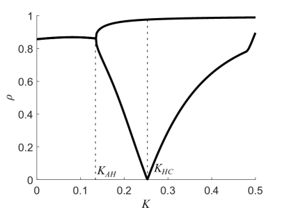
Figure 5: The bifurcation diagram for (3.3) with $0<\delta,\epsilon\ll 1$ (here, $\epsilon=0.1,\delta=0.01$). For families of periodic orbit, the largest and the smallest values of $\rho$ are indicated.

To get a first insight into the heteroclinic bifurcation, we numerically computed a Poincaré map for (2.11). Specifically, for values of $K$ near $K_{HC}$, we set up a cross section, $\Sigma$, intersecting the heteroclinic orbit (see a dashed line in plots a and b in Figure 6). Then we sampled initial conditions from the appropriate region of $\Sigma$ (around the point of intersection with $\Gamma^{0}$) and followed the corresponding trajectories until their first return to the chosen region of $\Sigma$ (see trajectories plotted in red of Figure 6a,b). Note that after the bifurcation the red trajectory makes a full revolution around the cylinder before returning back to $\Sigma$ (see Figure 6b). The Poincaré maps computed before and after the bifurcation are practically identical (see Figure 6c,d). Furthermore, the map shows a strong contraction of the vector field near the heteroclinic loops. The periodic orbits corresponding to the fixed points of the map shown in Figure 6c and d are shown in Figure 6e and f respectively. The two limit cycles approach heteroclinic loops $\overline{\Gamma^{0}\bigcup\Gamma^{-}}$ and $\overline{\Gamma^{0}\bigcup\Gamma^{+}}$ in Hausdorff distance as $K\to K_{HC}-0$ and $K\to K_{HC}+0$ respectively (see Figure 7). Both limit cycles are stable. Furthermore, numerically computed Poincaré maps do not show any effect of the heteroclinic bifurcation. These counterintuitive observations will be explained in the next section by the analysis of the nonlocal bifurcation taking place in (2.11).

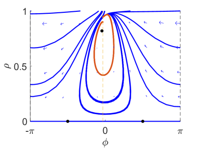
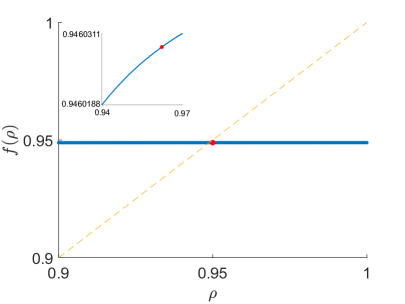
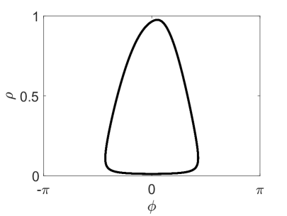
a  b 
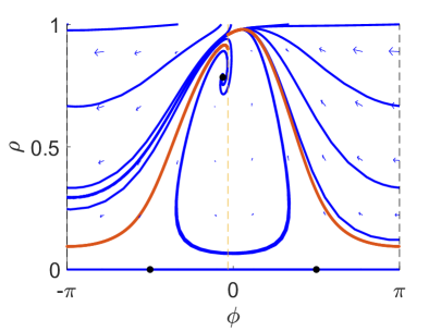
c  d 
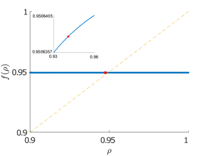
e  f 

Figure 6: a,b) The flow before and after the heteroclinic bifurcation ($K=0.23$ and $K=0.3$). The Poincaré section, $\phi=-0.1$, is indicated by the dashed line. The red trajectories illustrate the construction of the Poincaré map from $\rho=0.9$. c,d) The Poincaré map before and after the bifurcation: $K=0.251$ and $0.253$. The red dot on the Poincaré section marks the point of intersection with $W^{s}(S_{1})$. The Poincaré map is not defined at this point. e,f) The periodic solutions corresponding to the fixed points of the Poincaré map before $(K=0.251)$ and after $(K=0.253)$ the bifurcations. Both orbits are stable. In all figures, $\epsilon=0.1$ and $\delta=0.01$.

4 The boa constrictor bifurcation

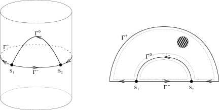
Figure 7: At at the heteroclinic bifurcation, two saddles, $S_{1}$ and $S_{2}$, are connected by three heteroclinic orbits $\Gamma^{0}$, $\Gamma^{-}$, and $\Gamma^{+}$. The sketch on the right explains the topology of the heteroclinic loops.

The main result of this section is given in the following theorem.

Theorem 4.1.

Consider a two-dimensional system on a cylinder

$$\dot{x}=f(x,\alpha),\;x\in({\mathbb{R}}/2\pi{\mathbb{Z}})\times{\mathbb{R}},\alpha\in{\mathbb{R}},$$ (4.1)

with smooth $f$. Suppose that for all $\alpha\in{\mathbb{R}}$ there are two saddles $S_{1}$ and $S_{2}$ connected with heteroclinic orbits $\Gamma^{+}$ and $\Gamma^{-}$ such that $\overline{\Gamma^{-}\bigcup\Gamma^{+}}$ is a noncontractible simple closed curve. In addition, for $\alpha=0$ there is another heteroclinic orbit $\Gamma_{0}$ connecting $S_{1}$ and $S_{2}$ such that $\overline{\Gamma^{-}\bigcup\Gamma_{0}}$ is a contractible simple closed curve (see Figure 7).

Let $\lambda_{1,2}^{s}:=\lambda_{1,2}^{s}(0)<0<\lambda_{1,2}^{u}:=\lambda_{1,2}^{u}(0)$ be the eigenvalues of the Jacobian $Df(S_{1,2},0)$. Recall that $\sigma_{1,2}=|\lambda_{1,2}^{s}|/\lambda^{u}_{1,2}$ is called the saddle number. Further, we assume

1. $\sigma:=\sigma_{1}\sigma_{2}\neq 1$,

2. $\beta^{\prime}(0)\neq 0$, where $\beta(\alpha)$ is a suitably defined split function (see below).

   Then for sufficiently small $|\alpha|$, there exists a small neighborhood of

   $$\Gamma:=\overline{\Gamma^{-}\bigcup\Gamma_{0}\bigcup\Gamma^{+}},$$

   which contains a unique limit cycle $\mathcal{P}_{\beta}$ bifurcating from $\Gamma$. Moreover, $\mathcal{P}_{\beta}$ is contractible for $\beta>0$ and noncontractible for $\beta<0$. It is stable if $\sigma>1$ and unstable otherwise.

Proof.

The proof employs a standard scheme for analyzing global bifurcations, which goes back to the proof of Andronov-Leontovich Theorem (cf. [24, Theorem 6.1]).

First, we introduce local cross sections $\Sigma_{1,2}$ and $\Pi_{1,2}^{\pm}$ near the saddles (see Fig. 8). Next we construct the following flow-defined maps

$$P_{1}: \Sigma_{1}\to\Pi_{1}^{-}\cup\Pi_{1}^{+},$$

$$P_{2}: \Sigma_{2}\to\Pi_{2}^{-}\cup\Pi_{2}^{+},$$

$$Q^{-}: \Pi_{1}^{-}\to\Pi_{2}^{-},$$

$$Q^{+}: \Pi_{1}^{+}\to\Pi_{2}^{+},$$

$$R: \Sigma_{2}\to\Sigma_{1}.$$

The near-to-saddle maps $P_{1}$ and $P_{2}$ capture the local dynamics near $S_{1}$ and $S_{2}$. $P_{1}$ and $P_{2}$ do not depend on $\alpha$ to leading order for small $|\alpha|$. Maps $Q^{-}$ and $Q^{+}$ are defined by the flow near $\Gamma^{-}$ and $\Gamma^{+}$. These maps do not depend on $\alpha$. Finally, $R$ is defined by the flow in a small vicinity of $W^{u}(S_{2})$.

On $\Sigma_{1}$ we select a system of coordinates such that $\xi=0$ corresponds to the point of intersection of $\Sigma_{1}$ and $W^{s}(S_{1})$. Then the coordinate $\xi$ of the point of intersection of $W^{u}(S_{2})$ with $\Sigma_{1}$ defines the split function:

$$\beta(\alpha):=\xi.$$

The near-saddle map $P_{1}$ is computed from the following linear system after a suitable change of coordinates near $S_{1}$ (cf. [18, Chapter 9])

$$\begin{split}\dot{\xi}&=\lambda_{1}^{u}\xi,\\ \dot{\eta}&=\lambda_{2}^{s}\eta.\end{split}$$ (4.2)

in the neighborhood of the origin with cross-sections $\Sigma_{1}=\{(\xi,1):\;\xi\in[-1,1]\}$, $\Pi_{1}^{-}=\{(1,\eta):\;\eta\in[0,1]\}$, and $\Pi_{1}^{+}=\{(-1,\eta):\;\eta\in[0,1]\}$ (see Fig. 9). A standard computation yields

$$P_{1}(\xi)=\xi^{\sigma_{1}}.$$

Similarly, we compute

$$P_{2}(\xi)=\xi^{\sigma_{2}}.$$

The global maps are given by

$$Q^{-}(\eta) =a^{-}\eta+O(\eta^{2}),$$ (4.3)

$$Q^{+}(\eta) =a^{+}\eta+O(\eta^{2}),$$ (4.4)

$$R(\xi) =\beta+a\xi+O(\xi^{2}),$$ (4.5)

where coefficients $a^{-},a^{+},$ and $a$ are positive and $\beta$ is the split function.

We can now compute the first return map

$$P=\left\{\begin{array}[]{ll}R\circ P_{2}\circ Q^{-}\circ P_{1},&\beta>0,\\ R\circ P_{2}\circ Q^{+}\circ P_{1},&\beta<0.\end{array}\right.$$ (4.6)

The combination of (4.3) and (4.6) yields

$$P(\xi)=\left\{\begin{array}[]{ll}\beta+a(a^{-})^{\sigma_{2}}\xi^{\sigma}+\mbox{higher order terms},&\beta>0,\\ \beta+a(a^{+})^{\sigma_{2}}\xi^{\sigma}+\mbox{higher order terms},&\beta<0.\end{array}\right.$$ (4.7)

From (4.7), one can see that $P$ has a fixed point $\bar{\xi}_{\beta}$ in a neighborhood of the origin for small $|\beta|\neq 0$. Further, $\bar{\xi}_{\beta}\beta>0$ for $\beta\neq 0$. Finally, $\bar{\xi}_{\beta}$ is stable if $\sigma>1$ (dissipative case) and is unstable if $\sigma<1$. ∎

Remark 4.2.

If $\sigma=1$ as in the case of (2.11) the stability of the bifurcating orbits is determined by the positive coefficients $a$, $a^{-}$, and $a^{+}$. Specifically, $\mathcal{P}_{\beta}$ is stable if $a(a^{-})^{\sigma_{2}}<1$ for $\beta>0$ and $a(a^{+})^{\sigma_{2}}$ for $\beta<0$. In this case, the stability of the orbit is determined by the degree of contraction produced by the global maps defined by the flow along the heteroclinic loops rather than by that of the local near-to-saddle maps. While obtaining analytical estimates of the contraction of the global maps requires tedious calculations, numerical first return maps in Figure 6c,d unequivocally demonstrate strong contraction.

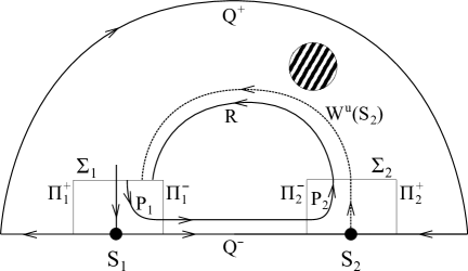
Figure 8: The first return map (see text for details).

Figure 9: The local (near the saddle) component of the first return map.

5 Collective dynamics

a b

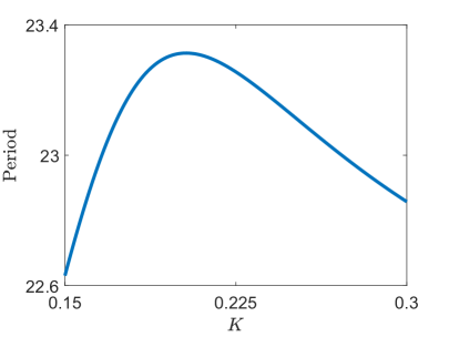
Figure 10: The period near the heteroclinic bifurcation for the systems with rescaled and original time (plots a and b respectively; cf. (2.11) and (2.10)). Parameters are $\epsilon=0.1$ and $\delta=0.01$.

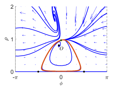
a  b 

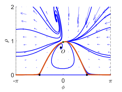
Figure 11: The phase portraits before (a) ($K=0.251$) and after (b) ($K=0.253$) the heteroclinic bifurcation show that the periodic trajectory (shown in red) passes near the unstable focus $O$ in each case. $O$ is close to $\{\rho=1\}$ because the system is still close to the Bogdanov-Takens bifurcation. The green dot indicates the region where the periodic trajectory spends most of the period. Other parameters are chosen as above: $\epsilon=0.1$, $\delta=0.01$.

Having analyzed the reduced system (2.11), we now return to the description of the collective dynamics of (1.1). The analysis in the previous two sections shows that the heteroclinic bifurcation separates two topologically distinct families of the limit cycles of (2.11) ${\mathcal{P}}_{K}$ for $K<K_{HC}$ and $K>K_{HC}$. In either case, ${\mathcal{P}}_{K}$ consists of a segment lying in $V_{c}=\{0\leq\rho<c\}$ for some $0<c\ll 1$ and an arc outside $V_{c}$ (see Fig. 7). Thus, in one cycle of oscillations the composition of the population of oscillators changes from high incoherence ($\rho\approx 0$) to high coherence ($\rho\approx 1$).

To estimate the duration of each of these phases and the period of oscillations note that the incoherent phase is determined by the time the periodic trajectory spends near the saddles, which can be easily estimated from (4.2). The trajectory of (4.2) starting from $(\beta,1)$ leaves the strip $|\xi|\leq 1$ after time

$$T_{1}\simeq\frac{1}{\lambda_{1}^{u}}\ln\frac{1}{|\beta|}.$$ (5.8)

Furthermore, at the time of exit

$$\eta=|\beta|^{\sigma_{1}}.$$ (5.9)

Thus, the trajectory enters the neighborhood of $S_{2}$ with $\eta=O\left(|\beta|^{\sigma_{1}}\right).$ From this, we can estimate the time it spends in the vicinity of $S_{2}$:

$$T_{2}\simeq\frac{\sigma_{1}}{\lambda_{1}^{u}}\ln\frac{1}{|\beta|}.$$ (5.10)

From (5.8) and (5.10), we estimate the period of oscillations near the heteroclinic bifurcation:

$$T\simeq\max\left\{\frac{1}{\lambda_{1}^{u}}\ln\frac{1}{|\beta|},\frac{\sigma_{1}}{\lambda_{2}^{u}}\ln\frac{1}{|\beta|}\right\}.$$ (5.11)

(see Fig. 10a).

After going back to the original time, for the oscillations in (2.10) we obtain:

$$T_{1}^{\prime} =\int_{0}^{T_{1}}\rho(\tau)d\tau\simeq\int_{0}^{T_{1}}e^{\lambda_{1}^{s}\tau}d\tau$$

$$\simeq\frac{1-C_{1}|\beta|^{\sigma_{1}}}{|\lambda_{1}^{s}|},$$

and similarly

$$T_{2}^{\prime}\simeq\frac{1-C_{1}|\beta|^{\sigma}}{|\lambda_{2}^{s}|}.$$

Thus, in the original time the period of oscillations remains finite (see Fig. 10 b). Furthermore, since the points on $W^{s}(S_{1})$ hit $S_{1}$ in finite time, the heteroclinic orbit reaches the saddle in finite time too. Recall that $\rho=0$ is the image of the origin in ${\mathbb{R}}^{2}$ under the polar coordinate transformation. The origin is not a fixed point of (2.9). Thus, the heteroclinic orbit of (2.11) for $K=K_{HC}$ corresponds to a periodic orbit of (2.9) passing through the origin in the cartesian coordinates (Figure 12). Thus, the family of periodic orbits $\mathcal{P}_{K},K>K_{AH}$ of (2.11) corresponds to a family of periodic orbits $\mathcal{Z}_{K}$ of (2.9). The period of $\mathcal{Z}_{K}$ achieves its maximum at $K=K_{HC}$ (see Fig. 10 b). The discrepancy in different locations of the maxima in plots a and b in Figure 10 is explained by the fact that we dropped higher order terms in (3.2).

Having described the ‘incoherent’ portion of the periodic orbit lying in a neighborhood of $\{\rho=0\}$, we now turn to the complimentary portion lying in a neighborhood of $\Gamma_{0}$ (see Fig. 11). First note that outside a small neighborhood of $\{\rho=0\}$ the rescaling of time no longer has a qualitative impact on the system’s dynamics. Further, on $\rho=1$ the vector field of (2.11) is pointed downward (see the $\rho$-equation in (2.11)). On the other hand, the unstable focus $O$ has not moved too far from $\{\rho=1\}$, where it emerged at the Bogdanov-Takens bifurcation (see Figure 11). Thus, $\Gamma_{0}$ has to pass in a region between $\{\rho=1\}$ and the unstable focus $O$ (Figure 11). This forces $\Gamma_{0}$ to pass close to $O$ where the vector field is very weak. Consequently, a significant portion of the period is spent near $\{\rho=1\}$, which correspond to the ‘coherent’ phase of oscillations. This results in an interesting scenario, for which the separation of the timescales in oscillations of the order parameter just before and after the heteroclinic bifurcation (Figure 1) is not due to the proximity of the heteroclinic bifurcation, as one would be tempted to assume, but rather to the proximity to the Bogdanov-Takens bifurcation. Thus, both the Bogdanov-Takens and the heteroclinic bifurcations have an impact on the qualitative features of the collective dynamics.

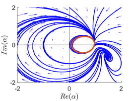
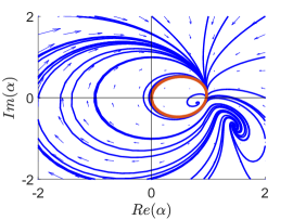
a  b  c 

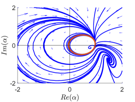
Figure 12: The phase portraits of (2.9) plotted in Cartesian coordinates. The middle plot (b) shows the periodic orbit passing through the origin. The two outer plots show the periodic orbits before (a) and after (c) this event. Parameters are chosen as above: $\epsilon=0.1$ and $\delta=0.01$, with $K=0.24,0.253,0.26$ from left to right.

We conclude with several remarks on the relation between (2.9) and (2.11). Recall that we switched to polar coordinates to be able to track the modulus and the argument of the order parameter, which capture macroscopic dynamics. The polar coordinate transformation is a diffeomorphism of ${\mathbb{R}}^{2}/\{(0,0)\}$ to ${\mathbb{R}}^{+}\times\operatorname{\mathbb{T}}$, but its is not a bijection at the origin. Consequently (2.9) and (2.11) are topologically equivalent only when restricted to ${\mathbb{R}}^{2}/\{(0,0)\}$ and ${\mathbb{R}}^{+}\times\operatorname{\mathbb{T}}$ respectively. In particular, the Andronov-Hopf and Bogdanov-Takens bifurcations describing local transformations of the vector field (2.11) in closed domains of ${\mathbb{R}}^{+}\times\operatorname{\mathbb{T}}$ translate automatically to the corresponding bifurcations of (2.9). On the other hand the heteroclinic bifurcation, which we analyzed for (2.11) involves the set $\rho=0$, which lies outside ${\mathbb{R}}^{+}\times\operatorname{\mathbb{T}}$. The heteroclinic orbit connecting $\Gamma^{0}$ (Figure 7) corresponds to a periodic orbit of (2.9) passing through the origin (Figure 12). This not a bifurcation of (2.9) as a vector field on ${\mathbb{R}}^{2}$, but it is a bifurcation on ${\mathbb{R}}^{2}/\{(0,0)\}$. This is a bifurcation, because a contractibe periodic orbit before hitting the origin becomes a noncontractibe one after this event. This is a border collision bifurcation. Clearly, this bifurcation is a consequence of our using the polar coordinate transformation, which is singular at the origin. Nonetheless, both the heteroclinic and the border collision bifurcations are relevant in the context of the macroscopic dynamics. While in the cartesian coordinates, the passing of the periodic orbit of (2.9) through the origin is a regular event, it represents a transition point in the description of the macroscopic dynamics. This is the point where the oscillations of the center of mass of the population of oscillators are transformed into rotations. At this point the amplitude and the period of the oscillations of the order parameter reach their respective maximal values, while the modulus of the order parameter reaches its minimal value. Note that the fast dips in the modulus of the order parameter can get arbitrarily close to $0$ provided that $n$ is large enough (Figure 7a). At the transition point, the oscillators are most dispersed as they undergo fast transitions between their successive stays near $\rho=1$ (Figure 7a). Therefore, the use of the polar coordinates in the analysis of (2.9) and the analysis of the heteroclinic bifurcation in the transformed system are essential for understanding macroscopic dynamics of the coupled system (1.1).

6 Discussion

In the present paper, we analyzed a modified KM with individual oscillators in the regime near a saddle-node on an invariant circle bifurcation. The modified model features a new type of collective dynamics with alternating phases of high and low coherence. Furthermore, the order parameter exhibits slow-fast oscillations, which reveal a pronounced separation of timescales in collective dynamics. For the most part of the period the value of the order parameter is close to $1$ corresponding to the coherent phase. The long periods of coherence are punctuated by brief intervals of highly incoherent collective dynamics. The Ott-Antonsen reduction and a careful analysis of the reduced system show that the salient features of the collective dynamics are explained by the model’s proximity to a local Bogdanov-Takens bifurcation and a nonlocal heteroclinic bifurcation. In contrast to previously studied cases, where one limit cycle or two limit cycles of opposite stability appear in a bifurcation of a homoclinic/heteroclinic contour (cf. [3, 24, 25, 13]), the heteroclinic bifurcation for the system at hand generates a limit cycles on each side of the bifurcation. These limit cycles are topologically distinct (contractible versus noncontractible) and are either both stable or both unstable.

Acknowledgements. This work grew out of AP’s Research Co-op at Drexel University. GSM and AP were supported in part by NSF grant DMS 2009233 (to GSM). MSM was supported by a Support of Scholarly Activities Grant at The College of New Jersey.

Data availability statement. Data sharing is not applicable to this article as no datasets were generated or analyzed during the current study.

References

- [1] J.A. Acebrón and L.L. Bonilla, Asymptotic description of transients and synchronized states of globally coupled oscillators, Physica D: Nonlinear Phenomena 114 (1998), no. 3, 296–314.
- [2] V. I. Arnold, Lectures on bifurcations and versal families, Uspehi Mat. Nauk 27 (1972), no. 5(167), 119–184, A series of articles on the theory of singularities of smooth mappings.
- [3] V. I. Arnold, V. S. Afrajmovich, Yu. S. Il′ yashenko, and L. P. Shil′ nikov, Bifurcation theory and catastrophe theory, Springer-Verlag, Berlin, 1999, Translated from the 1986 Russian original by N. D. Kazarinoff, Reprint of the 1994 English edition from the series Encyclopaedia of Mathematical Sciences [ıt Dynamical systems. V, Encyclopaedia Math. Sci., 5, Springer, Berlin, 1994; MR1287421 (95c:58058)].
- [4] D. K. Arrowsmith and C. M. Place, An introduction to dynamical systems, Cambridge University Press, Cambridge, 1990.
- [5] R. I. Bogdanov, Versal deformation of a singular point of a vector field on the plane in the case of zero eigenvalues, Funkcional Anal. i Priložen. 9 (1975), no. 2, 63.
- [6] Hayato Chiba, A proof of the Kuramoto conjecture for a bifurcation structure of the infinite-dimensional Kuramoto model, Ergodic Theory Dynam. Systems 35 (2015), no. 3, 762–834.
- [7] Hayato Chiba and Georgi S. Medvedev, The mean field analysis of the Kuramoto model on graphs I. The mean field equation and transition point formulas, Discrete Contin. Dyn. Syst. 39 (2019), no. 1, 131–155.
- [8] Hayato Chiba, Georgi S. Medvedev, and Matthew S. Mizuhara, Bifurcations in the Kuramoto model on graphs, Chaos 28 (2018), no. 7, 073109, 10.
- [9] Lauren M. Childs and Steven H. Strogatz, Stability diagram for the forced Kuramoto model, Chaos 18 (2008), no. 4, 043128, 9.
- [10] Helge Dietert, Stability and bifurcation for the Kuramoto model, J. Math. Pures Appl. (9) 105 (2016), no. 4, 451–489.
- [11] R. L. Dobrušin, Vlasov equations, Funktsional. Anal. i Prilozhen. 13 (1979), no. 2, 48–58, 96.
- [12] Dawid Dudkowski, Yuri Maistrenko, and Tomasz Kapitaniak, Occurrence and stability of chimera states in coupled externally excited oscillators, Chaos 26 (2016), no. 11, 116306, 9.
- [13] A. V. Dukov, Bifurcations of the ‘heart’ polycycle in generic 2-parameter families, Trans. Moscow Math. Soc. 79 (2018), 209–229.
- [14] Bard Ermentrout, Type I Membranes, Phase Resetting Curves, and Synchrony, Neural Computation 8 (1996), no. 5, 979–1001.
- [15] George Bard Ermentrout and Nancy Kopell, Parabolic bursting in an excitable system coupled with a slow oscillation, SIAM J. Appl. Math. 46 (1986), no. 2, 233–253.
- [16] John Guckenheimer and Philip Holmes, Nonlinear oscillations, dynamical systems, and bifurcations of vector fields, Applied Mathematical Sciences, vol. 42, Springer-Verlag, New York, 1990, Revised and corrected reprint of the 1983 original.
- [17] Frank C. Hoppensteadt and Eugene M. Izhikevich, Weakly connected neural networks, Applied Mathematical Sciences, vol. 126, Springer-Verlag, New York, 1997.
- [18] Yu. Ilyashenko and Weigu Li, Nonlocal bifurcations, Mathematical Surveys and Monographs, vol. 66, American Mathematical Society, Providence, RI, 1999.
- [19] Benjamin Jüttner, Christian Henriksen, and Erik A. Martens, Birth and destruction of collective oscillations in a network of two populations of coupled type 1 neurons, Chaos 31 (2021), no. 2, Paper No. 023141, 12.
- [20] Vladimir Klinshov and Igor Franović, Mean-field dynamics of a random neural network with noise, Phys. Rev. E 92 (2015), 062813.
- [21] Vladimir Klinshov and Igor Franović, Two scenarios for the onset and suppression of collective oscillations in heterogeneous populations of active rotators, Phys. Rev. E 100 (2019), 062211.
- [22] Y. Kuramoto and D. Battogtokh, Coexistence of coherence and incoherence in nonlocally coupled phase oscillators, Nonlinear Phenomena in Complex Systems 5 (2002), 380–385.
- [23] Yoshiki Kuramoto, Self-entrainment of a population of coupled non-linear oscillators, International Symposium on Mathematical Problems in Theoretical Physics (Kyoto Univ., Kyoto, 1975), Springer, Berlin, 1975, pp. 420–422. Lecture Notes in Phys., 39.
- [24] Yuri A. Kuznetsov, Elements of applied bifurcation theory, third ed., Applied Mathematical Sciences, vol. 112, Springer-Verlag, New York, 2004.
- [25] Yuri A. Kuznetsov and Joost Hooyman, Bifurcations of heteroclinic contours in two-parameter planar systems: Overview and explicit examples, International Journal of Bifurcation and Chaos 31 (2021), no. 12, 2130036.
- [26] Luis F. Lafuerza, Pere Colet, and Raul Toral, Nonuniversal results induced by diversity distribution in coupled excitable systems, Phys. Rev. Lett. 105 (2010), 084101.
- [27] Carlo R. Laing, The dynamics of chimera states in heterogeneous Kuramoto networks, Phys. D 238 (2009), no. 16, 1569–1588.
- [28] , Derivation of a neural field model from a network of theta neurons, Phys. Rev. E 90 (2014), 010901.
- [29] Georgi S. Medvedev and Svitlana Zhuravytska, The geometry of spontaneous spiking in neuronal networks, J. Nonlinear Sci. 22 (2012), no. 5, 689–725.
- [30] Simbarashe Nkomo, Mark R. Tinsley, and Kenneth Showalter, Chimera and chimera-like states in populations of nonlocally coupled homogeneous and heterogeneous chemical oscillators, Chaos 26 (2016), no. 9, 094826, 10.
- [31] O. E. Omel’chenko, The mathematics behind chimera states, Nonlinearity 31 (2018), no. 5, R121–R164.
- [32] Oleh Omel’chenko and Carlo R. Laing, Collective states in a ring network of theta neurons, Proc. A. 478 (2022), no. 2259, Paper No. 817, 23.
- [33] Edward Ott and Thomas M. Antonsen, Low dimensional behavior of large systems of globally coupled oscillators, Chaos 18 (2008), no. 3, 037113, 6.
- [34] , Long time evolution of phase oscillator systems, Chaos 19 (2009), no. 2, 023117, 5.
- [35] Mark J. Panaggio and Daniel M. Abrams, Chimera states: coexistence of coherence and incoherence in networks of coupled oscillators, Nonlinearity 28 (2015), no. 3, R67–R87.
- [36] Lennart Schmidt, Konrad Schönleber, Katharina Krischer, and Vladimir García-Morales, Coexistence of synchrony and incoherence in oscillatory media under nonlinear global coupling, Chaos 24 (2014), no. 1, 013102, 7.
- [37] Shigeru Shinomoto and Yoshiki Kuramoto, Phase Transitions in Active Rotator Systems, Progress of Theoretical Physics 75 (1986), no. 5, 1105–1110.
- [38] Steven H. Strogatz, From Kuramoto to Crawford: exploring the onset of synchronization in populations of coupled oscillators, Phys. D 143 (2000), no. 1-4, 1–20, Bifurcations, patterns and symmetry.
- [39] Steven H. Strogatz and Renato E. Mirollo, Stability of incoherence in a population of coupled oscillators, J. Statist. Phys. 63 (1991), no. 3-4, 613–635.
- [40] Steven H. Strogatz, Renato E. Mirollo, and Paul C. Matthews, Coupled nonlinear oscillators below the synchronization threshold: relaxation by generalized Landau damping, Phys. Rev. Lett. 68 (1992), no. 18, 2730–2733.
- [41] Floris Takens, Singularities of vector fields, Inst. Hautes Études Sci. Publ. Math. (1974), no. 43, 47–100.
- [42] C. J. Tessone, A. Sciré, R. Toral, and P. Colet, Theory of collective firing induced by noise or diversity in excitable media, Phys. Rev. E 75 (2007), 016203.
- [43] D.A. Wiley, S.H. Strogatz, and M. Girvan, The size of the sync basin, Chaos 16 (2006), no. 1, 015103, 8.
- [44] M. A. Zaks, A. B. Neiman, S. Feistel, and L. Schimansky-Geier, Noise-controlled oscillations and their bifurcations in coupled phase oscillators, Phys. Rev. E 68 (2003), 066206.