Enhancing Adversarial Robustness for Deep Metric Learning

Abstract

Owing to security implications of adversarial vulnerability, adversarial robustness of deep metric learning models has to be improved. In order to avoid model collapse due to excessively hard examples, the existing defenses dismiss the min-max adversarial training, but instead learn from a weak adversary inefficiently. Conversely, we propose Hardness Manipulation to efficiently perturb the training triplet till a specified level of hardness for adversarial training, according to a harder benign triplet or a pseudo-hardness function. It is flexible since regular training and min-max adversarial training are its boundary cases. Besides, Gradual Adversary, a family of pseudo-hardness functions is proposed to gradually increase the specified hardness level during training for a better balance between performance and robustness. Additionally, an Intra-Class Structure loss term among benign and adversarial examples further improves model robustness and efficiency. Comprehensive experimental results suggest that the proposed method, although simple in its form, overwhelmingly outperforms the state-of-the-art defenses in terms of robustness, training efficiency, as well as performance on benign examples.

1 Introduction

Given a set of data points, a metric gives a distance value between each pair of them. Deep Metric Learning (DML) aims to learn such a metric between two inputs (e.g., images) leveraging the representational power of deep neural networks. As an extensively studied task [27, 21], DML has a wide range of applications such as image retrieval [37] and face recognition [28, 6], and widely influences some other areas such as self-supervised learning [21].

Despite the advancements in this field thanks to deep learning, recent studies find DML models vulnerable to adversarial attacks, where imperceptible perturbations can incur unexpected retrieval result, or covertly change the rankings [53, 54]. Such vulnerability raises security, safety, and fairness concerns in the DML applications. For example, impersonation or recognition evasion are possible on a vulnerable DML-based face-identification system. To counter the attacks (i.e., mitigating the vulnerability), the adversarial robustness of DML models has to be improved via defense.

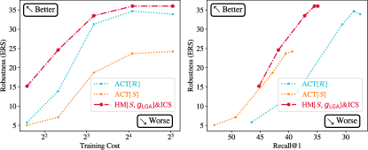
Figure 1: Comparison in robustness, training cost, and recall@1 between our method (i.e., “HM[$\mathcal{S},g_{\mathsf{LGA}}$]&ICS”) and the state-of-the-art method (i.e., “ACT[$\mathcal{R}$]” and “ACT[$\mathcal{S}$]”) on the CUB Dataset.

Existing defense methods [53, 55] are adversarial training-based, inspired by Madry’s min-max adversarial training [20] because it is consistently one of the most effective methods for classification task. Specifically, Madry’s method involves a inner problem to maximize the loss by perturbing the inputs into adversarial examples, and an outer problem to minimize the loss by updating the model parameters. However, in order to avoid model collapse due to excessively hard examples, the existing DML defenses refrain from directly adopting such min-max paradigm, but instead replace the inner problem to indirectly increase the loss value to a certain level, which suffers from low efficiency and weak adversary (and hence weak robustness). Since training cost is already a serious issue of adversarial training, the efficiency in gaining higher adversarial robustness under a lower budget is inevitable and important for DML defense.

Inspired by previous works [53, 55], we conjecture that an appropriate adversary for the inner maximization problem should increase the loss to an “intermediate” point between that of benign examples (i.e., unperturbed examples) and the theoretical upper bound. Such point should be reached by an efficient adversary directly. Besides, we speculate the triplet sampling strategy has a key impact in adversarial training, because it is also able to greatly influence the mathematical expectation of loss even without adversarial attack.

In this paper, we first define the “hardness” of a sample triplet as the difference between the anchor-positive distance and anchor-negative distance. Then, Hardness Manipulation (HM) is proposed to adversarially perturb a given sample triplet and increase its hardness into a specified destination hardness level for adversarial training. The objective of HM is to minimize the L-$2$ norm of the thresholded difference between the hardness of the given sample triplet and the specified destination hardness. HM is flexible as regular training and min-max adversarial training [20] can be expressed as its boundary cases, as shown in Fig. 2. Mathematically, when the HM objective is optimized using Projected Gradient Descent [20], the sign of its gradient with respect to the adversarial perturbation is the same as that of directly maximizing the loss. Thus, the optimization of HM objective can be interpreted as a direct and efficient maximization process of the loss which stops halfway at the specified destination hardness level, i.e., the aforementioned “intermediate” point.

Then, how hard should such “destination hardness” be? Recall that the model is already prone to collapse with excessively hard benign triplets [28], let alone adversarial examples. Thus, intuitively, the destination hardness can be the hardness of another benign triplet which is moderately harder than the given triplet (e.g., a Semihard [28] triplet). However, in the late phase of training, the expectation of the difference between such destination hardness and that of the given triplet will be small, leading to weak adversarial examples and inefficient adversarial learning. Besides, strong adversarial examples in the early phase of training may also hinder the model from learning good embeddings, and hence influence the performance on benign examples. In particular, a better destination hardness should be able to balance the training objectives in the early and late phases of training.

To this end, Gradual Adversary, a family of pseudo-hardness functions is proposed, which can be used as the destination hardness. A function that leads to relatively weak and relatively strong adversarial examples, respectively in the early and late phase of training belongs to this family. As an example, we design a “Linear Gradual Adversary” (LGA) function as the linearly scaled negative triplet margin, incorporating a strong prior that the destination hardness should remain Semihard based on our empirical observation.

Additionally, it is noted that a sample triplet will be augmented into a sextuplet (both benign and adversarial examples) during adversarial training. In this case, the intra-class structure can be enforced, which has been neglected by existing methods. Since some existing attacks aim to change the sample rankings in the same class [53], we propose a simple intra-class structure loss term for adversarial training, which is expected to further improve adversarial robustness.

Comprehensive experiments are conducted on three commonly used DML datasets, namely CUB-200-2011 [40], Cars-196 [14], and Stanford Online Product [22]. The proposed method overwhelmingly outperforms the state-of-the-art defense in terms of robustness, training efficiency, as well as the performance on benign examples.

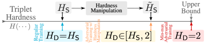
Figure 2: Flexibility of hardness manipulation. Regular training and min-max adversarial training are its boundary cases.

In summary, our contributions include proposing:

1. Hardness Manipulation (HM) as a flexible and efficient tool to create adversarial example triplets for subsequent adversarial training of a DML model.

2. Linear Gradual Adversary (LGA) as a Gradual Adversary, i.e., a pseudo-hardness function for HM, which incorporates our empirical observations and can balance the training objectives during the training process.

3. Intra-Class Structure (ICS) loss term to further improve model robustness and adversarial training efficiency, while such structure is neglected by existing defenses.

2 Related Works

Adversarial Attack. Szegedy et al. [31] find misclassification of DNN can be triggered by an imperceptible adversarial perturbation to the input image. Ian et al. [8] attribute the reason to DNN being locally linear with respect to the adversarial perturbation. Subsequent first-order gradient-based methods can compromise the DNNs more effectively under the white-box assumption [15, 20, 4, 46]. In contrast, black-box attacks have been explored by query-based methods [12, 35] and transferability-based methods [45], which are more practical for real-world scenarios.

Adversarial Defense. Various defenses are proposed to counter the attacks. However, defenses incurring gradient masking lead to a false sense of robustness [1]. Defensive distillation [24] is compromised in [3]. Ensemble of weak defenses is not robust [10]. Other defenses such as input preprocessing [25], or randomization [19] are proposed. But many of them are still susceptible to adaptive attacks [33]. Of all defenses, adversarial training [20] consistently remains to be one of the most effective methods [38, 51, 5, 30, 49, 11, 43, 48, 2, 44], but suffers from high training cost [29, 41, 47], performance drop on benign examples [34, 50, 18], and overfitting on adversarial examples [23, 26].

Deep Metric Learning. A wide range of applications such as image retrieval [37], cross-modal retrieval [52], and face recognition [28] can be formulated as a DML problem. A well-designed loss function and a proper sampling method are crucial for DML performance [21]. For instance, the classical triplet loss [28] could reach state-of-the-art performance with an appropriate sampling strategy [27].

Attacks in DML. DML has been found vulnerable to adversarial attacks as well [53, 54, 55], which raises concerns on safety, security, or fairness for a DML application. The existing attacks aim to completely subvert the image retrieval results [17, 36, 7, 39, 32, 16], or covertly alter the top-ranking results without being abnormal [53, 54].

Defenses in DML. Unlike attacks, defenses are less explored. Embedding Shifted Triplet (EST) [53] is an adversarial training method using adversarial examples with maximized embedding move distance off their original locations. The state-of-the-art method, i.e., Anti-Collapse Triplet (ACT) [55] forces the model to separate collapsed positive and negative samples apart in order to learn robust features. However, both EST and ACT suffer from low efficiency as the inner problem is replaced into an indirect adversary.

3 Our Approach

In DML [27, 21], a function $\phi:\mathcal{X}{\mapsto}\Phi\subseteq\mathbb{R}^{D}$ is learned to map data points ${\bm{X}}\in\mathcal{X}$ into an embedding space $\Phi$, which is usually normalized to the real unit hypersphere for regularization. With a predefined distance function $d(\cdot,\cdot)$, which is usually the Euclidean distance, we can measure the distance between ${\bm{X}}_{i}$ and ${\bm{X}}_{j}$ as $d_{\phi}({\bm{X}}_{i},{\bm{X}}_{j})=d(\phi({\bm{X}}_{i}),\phi({\bm{X}}_{j}))$. Typically, the triplet loss [28] can be used to learn the embedding function, and it could reach the state-of-the-art performance with an appropriate triplet sampling strategy [27].

Given a triplet of anchor, positive, negative images, i.e., ${\bm{A}},{\bm{P}},{\bm{N}}\in\mathcal{X}$, we can calculate their embeddings with $\phi(\cdot)$ as ${\bm{a}},{\bm{p}},{\bm{n}}$, respectively. Then triplet loss [28] is defined as:

$$L_{\text{T}}({\bm{a}},{\bm{p}},{\bm{n}};\gamma)=\max(0,d({\bm{a}},{\bm{p}})-d({\bm{a}},{\bm{n}})+\gamma),$$ (1)

where $\gamma$ is a predefined margin parameter. To attack the DML model, an imperceptible adversarial perturbation ${\bm{r}}\in\Gamma$ is added to the input image ${\bm{X}}$, where $\Gamma=\{{\bm{r}}|{\bm{X}}+{\bm{r}}\in\mathcal{X},\|{\bm{r}}\|_{p}\leq\varepsilon\}$, so that its embedding vector $\tilde{{\bm{x}}}=\phi({\bm{X}}+{\bm{r}})$ will be moved off its original location towards other positions to achieve the attacker’s goal. To defend against the attacks, the DML model can be adversarially trained to reduce the effect of attacks [53, 55]. The most important metrics for a good defense are adversarial robustness, training efficiency, and performance on benign examples.

3.1 Hardness Manipulation

Given an image triplet (${\bm{A}}$, ${\bm{P}}$, ${\bm{N}}$) sampled with a certain sampling strategy (e.g., Random) within a mini-batch, we define its “hardness” as a scalar which is within $[-2,2]$:

$$H({\bm{A}},{\bm{P}},{\bm{N}})=d_{\phi}({\bm{A}},{\bm{P}})-d_{\phi}({\bm{A}},{\bm{N}}).$$ (2)

Clearly, it is an internal part of the triplet loss. For convenience, we call this triplet (${\bm{A}}$, ${\bm{P}}$, ${\bm{N}}$) as “source triplet”, and its corresponding hardness value as “source hardness”, denoted as $H_{\mathsf{S}}$.

Then, Hardness Manipulation (HM) aims to increase the source hardness $H_{\mathsf{S}}$ into a specified “destination hardness” $H_{\mathsf{D}}$, by finding adversarial examples of the source triplet, i.e., $({\bm{A}}{+}{{\bm{r}}}_{a},{\bm{P}}{+}{{\bm{r}}}_{p},{\bm{N}}{+}{{\bm{r}}}_{n})$, where $({{\bm{r}}}_{a},{{\bm{r}}}_{p},{{\bm{r}}}_{n})$ are the adversarial perturbations. Denoting the hardness of the adversarially perturbed source triplet as $\tilde{H}_{\mathsf{S}}$, i.e., $\tilde{H}_{\mathsf{S}}=H({\bm{A}}{+}{{\bm{r}}}_{a},{\bm{P}}{+}{{\bm{r}}}_{p},{\bm{N}}{+}{{\bm{r}}}_{n})$, the HM is implemented as:

$$\hat{{\bm{r}}}_{a},\hat{{\bm{r}}}_{p},\hat{{\bm{r}}}_{n}=\operatorname*{arg\,min}_{{\bm{r}}_{a},{\bm{r}}_{p},{\bm{r}}_{n}}\big{\|}\max(0,H_{\mathsf{D}}-\tilde{H}_{\mathsf{S}})\big{\|}_{2}^{2}.$$ (3)

The $\max(0,\cdot)$ part in Eq. 3 truncates the gradient when $\tilde{H}_{\mathsf{S}}>H_{\mathsf{D}}$, automatically stopping the optimization, because $\tilde{H}_{\mathsf{S}}$ is not desired to be reduced once it exceeds $H_{\mathsf{D}}$. Eq. 3 is written in the L-$2$ norm form instead of the standard Mean Squared Error because HM can be directly extended into vector form for a mini-batch. The optimization problem can be solved by Projected Gradient Descent (PGD) [20]. And the resulting adversarial examples are used for adversarially training the DML model with $L_{\text{T}}(\phi({\bm{A}}+\hat{{\bm{r}}}_{a}),\phi({\bm{P}}+\hat{{\bm{r}}}_{p}),\phi({\bm{N}}+\hat{{\bm{r}}}_{n}))$. The overall procedure of HM is illustrated in Fig. 3. For convenience, we abbreviate the adversarial training with adversarial examples created through this way as “$\text{HM}[H_{\mathsf{S}},H_{\mathsf{D}}]$” in this paper.

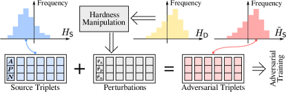
Figure 3: Illustration of hardness manipulation.

Note, in the PGD case, the sign of negative gradient of the HM objective w.r.t. an adversarial perturbation ${\bm{r}}$ is equivalent to the sign of gradient for directly maximizing $\tilde{H}_{\mathsf{S}}$ (hence maximizing $L_{\text{T}}$) when $H_{\mathsf{D}}>\tilde{H}_{\mathsf{S}}$, i.e.,

$$\Delta{\bm{r}}= \operatorname{sign}\big{\{}-\frac{\partial}{\partial{\bm{r}}}\big{\|}\max(0,H_{\mathsf{D}}-\tilde{H}_{\mathsf{S}})\big{\|}_{2}^{2}\big{\}}$$ (4)

$$= \operatorname{sign}\big{\{}2(H_{\mathsf{D}}-\tilde{H}_{\mathsf{S}})\frac{\partial}{\partial{\bm{r}}}\tilde{H}_{\mathsf{S}}\big{\}}=\operatorname{sign}\big{\{}\frac{\partial}{\partial{\bm{r}}}\tilde{H}_{\mathsf{S}}\big{\}}.$$ (5)

The perturbation ${\bm{r}}$ is updated as ${\bm{r}}\leftarrow\text{Proj}_{\Gamma}\{{\bm{r}}+\alpha\Delta{\bm{r}}\}$ by PGD for $\eta$ steps with a step size $\alpha$, where the “Proj” operator clips the result into the $\Gamma$ set. Thus, the optimization of HM objective can be interpreted as direct maximization of $\tilde{H}_{\mathsf{S}}$, which discontinues very early once it exceeds $H_{\mathsf{D}}$. With HM, the model can learn from an efficient adversary.

Since the same $\Delta{\bm{r}}$ can be used for both minimizing the HM objective and maximizing the triplet loss, one potential advantage of HM is that the gradients during the training process can be reused for creating adversarial examples for much faster adversarial training, according to Free Adversarial Training [29]. We leave this for future exploration.

Destination Hardness. $\text{HM}[H_{\mathsf{S}},H_{\mathsf{D}}]$ is flexible as various types of $H_{\mathsf{D}}$ can be specified, e.g., a constant, the hardness of another benign triplet, or a pseudo-hardness function. The case of maximizing the triplet loss is equivalent to $\text{HM}[H_{\mathsf{S}},2]$, where $2$ is the upper bound of hardness, while $\text{HM}[H_{\mathsf{S}},H_{\mathsf{S}}]$ is regular DML training, as shown in Fig. 2.

As pushing $\tilde{H}_{\mathsf{S}}$ towards the upper bound will easily render model collapse, a valid $H_{\mathsf{D}}$ should be chosen within the interval $[H_{\mathsf{S}},2]$. Thus, intuitively, $H_{\mathsf{D}}$ can be the hardness of another benign triplet (with the same anchor) sampled with a strategy with a higher hardness expectation, i.e., $E[H_{\mathsf{D}}]>E[H_{\mathsf{S}}]$. Or at least the $\text{Var}[H_{\mathsf{D}}]$ of another benign triplet has to be large enough (for a small portion of triplets $H_{\mathsf{D}}>H_{\mathsf{S}}$) in order to create a notable number of valid adversarial examples. For instance, $H_{\mathsf{D}}$ can be the hardness of a Semihard [28] triplet when the source triplet is sampled with Random sampler. Predictably, the model performance will be significantly influenced by the triplet sampling strategies we chose for $H_{\mathsf{D}}$ in this case. For convenience of further discussion, we denote the hardness of a Random, Semihard, and Softhard triplets as $\mathcal{R}$, $\mathcal{M}$, $\mathcal{S}$, respectively.

If we have a strong prior knowledge on what the destination hardness should be, then we can even use a pseudo-hardness function $g(\cdot)$, i.e., a customized scalar function.

3.2 Gradual Adversary

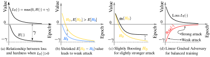
Figure 4: Illustration of (linear) gradual adversary.

Even if $H_{\mathsf{D}}$ is calculated from another triplet harder than the source triplet, the adversarial example may become weak in the late phase of training. The optimizer aims to reduce the expectation of loss $E[L_{\text{T}}]$ towards zero as possible over the distribution of triplets, and thus the $E[H]$ of any given triplet will tend to $-\gamma$, reducing the hardness of adversarial triplets from HM as $E[H_{\mathsf{D}}-H_{\mathsf{S}}]$ decreases accordingly. Weakened adversarial examples are insufficient for robustness.

Intuitively, such deficiency can be alleviated with a pseudo-hardness function that slightly increases the value of $H_{\mathsf{D}}$ in the late phase of training. Denoting the loss value from the previous training iteration as $\ell_{t-1}$, we first normalize it into $[0,1]$ as $\bar{\ell}_{t-1}=\min(u,\ell_{t-1})/u$, where $u$ is a manually specified constant. Then we can linearly shift the $E[H_{\mathsf{D}}]$ by a scaled constant $\xi$, i.e.,

$$g_{\mathsf{B}}(H_{\mathsf{D}};\xi,\bar{\ell}_{t-1})=H_{\mathsf{D}}+\xi\cdot(1-\bar{\ell}_{t-1}).$$ (6)

The deficiency can be alleviated in $\text{HM}[H_{\mathsf{S}},g_{\mathsf{B}}(H_{\mathsf{D}})]$.

Apart from the deficiency in the late phase of training, we speculate that relatively strong adversarial examples may hinder the model from learning good embedding space for the benign examples in the very early phase of training, hence influence the model performance on benign examples.

Thus, $H_{\mathsf{D}}$ should lead to (1) relatively weak adversarial examples in the early training phase (indicated by a large loss value), and (2) relatively strong adversarial examples in the late training phase (indicated by a small loss value), in order to automatically balance the training objectives (i.e., performance on benign examples v.s. robustness). A satisfactory pseudo-hardness function is a “Gradual Adversary”.

As an example, we propose a “Linear Gradual Adversary” (LGA) pseudo-hardness function that is independent to any benign triplets, incorporating our empirical observation that $H_{\mathsf{D}}$ should remain Semihard [28], as follows:

$$g_{\mathsf{LGA}}(\bar{\ell}_{t-1})=-\gamma\cdot\bar{\ell}_{t-1}~{}\in[-\gamma,0].$$ (7)

Our empirical observation is obtained from Sec. 4.1. And the training objectives, namely performance on benign examples and robustness will be automatically balanced in $\text{HM}[H_{\mathsf{S}},g_{\mathsf{LGA}}]$, leading to a better eventual overall performance, as illustrated in Fig. 4. More complicated or non-linear pseudo-hardness functions are left for future study.

3.3 Intra-Class Structure

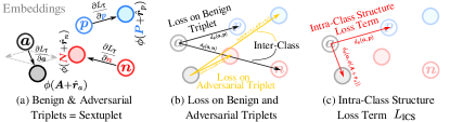
Figure 5: Illustration of intra-class structure loss term.

During adversarial training with HM, the adversarial counterpart of each given sample triplet is fed to the model, and the triplet loss will enforce a good inter-class structure. Since the anchor, positive sample, and their adversarial counterpart belongs to the same class, it should be noted that the intra-class structure can be enforced as well, but this has been neglected by the existing DML defenses. Intra-class structure is also important for robustness besides the inter-class structure, because the attack may attempt to change the rankings of samples in the same class [53].

We propose an additional loss function term to enforce such intra-class structure, as shown in Fig. 5. Specifically, the anchor ${\bm{a}}$ and its adversarial counterpart are separated from the positive sample ${\bm{p}}$ by reusing the triplet loss, i.e.,

$$L_{\text{ICS}}=\lambda\cdot L_{\text{T}}({\bm{a}},\phi({\bm{A}}+\hat{{\bm{r}}}_{a}),{\bm{p}};0),$$ (8)

where $\lambda$ is a constant weight for this loss term, and the margin is set as zero to avoid negative effect. The $L_{\text{ICS}}$ term can be appended to the loss function for adversarial training.

4 Experiments

To validate our defense method, we conduct experiments on three commonly used DML datasets: CUB-200-2011 (CUB) [40], Cars-196 (CARS) [14], and Stanford-Online-Product (SOP) [22]. We follow the same experimental setup as that used in the state-of-the-art defense work [55] and standard DML [27] for ease of comparison.

Statistics	Random	Semihard	Softhard	Distance	Hardest
$E[H]$	$-0.164$	$-0.126$	$-0.085$	$0.043$	$0.044$
$\text{Var}[H]$	$0.00035$	$0.00013$	$0.00122$	$0.00021$	$0.00021$

Table 1: Mean & variance of hardness w/ various triplet samplers. Calculated as the average statistics over $1000$ mini-batches from the CUB dataset with an imagenet-initialized RN18 model.

Specifically, we (adversarially) train ImageNet-initialized ResNet-18 (RN18) [9] with the output dimension of the last layer changed to $N{=}512$. The margin $\gamma$ in the triplet loss is $0.2$. Adam [13] optimizer is used for parameter updates, with a learning rate of $1.0{\times}10^{-3}$ for $150$ epochs, and a mini-batch size of $112$. Adversarial examples are created within $\Gamma$ with $\varepsilon{=}8/255$ and $p{=}\infty$, using PGD [20] with step size $\alpha{=}1/255$ and a default maximum step number $\eta{=}8$. The parameter $u$ is equal to $\gamma$, much less than the loss upper bound in order to avoid excessive hardness boost in $g_{\mathsf{B}}$ and $g_{\mathsf{LGA}}$. Parameter $\lambda$ for $L_{\text{ICS}}$ is $0.5$ by default ($0.05$ on SOP).

The model performance on the benign (i.e., unperturbed) examples is measured in terms of Recall@1 (R@1), Recall@2 (R@2), mAP and NMI following [27, 55]. The adversarial robustness of a model is measured in Empirical Robustness Score (ERS) [55], a normalized score (the higher the better) from a collection of (simplified white-box) attacks against DML, which are optimized with PGD ($\eta=32$ for strong attack). Since adversarial training is not “gradient masking” [1], the performance of white-box attack can be regarded as the upper bound of the black-box attacks, and thus a model that is empirically robust to the collection of white-box attacks is expected to be robust in general.

Concretely, the collection of attacks for ERS include: (1) CA+, CA-, QA+ and QA- [53], which move some selected candidates towards the topmost or bottommost part of ranking list; (2) TMA [32] which increases the cosine similarity between two arbitrary samples; (3) ES [53, 7], which moves the embedding of a sample off its original position as distant as possible; (4) LTM [36], which perturbs the ranking result by minimizing the distance of unmatched pairs while maximizing the distance of matched pairs; (5) GTM [55], which minimizes the distance between query and the closest unmatching sample. (6) GTT [55], aims to move the top-$1$ candidate out of the top-$4$ retrieval results, which is simplified from [17]. The setup of all the attacks for robustness evaluation is unchanged from [55] for fair comparison. Further details of these attacks can be found in [55].

4.1 Selection of Source & Destination Hardness

	Random		Semihard		Softhard		Distance		Hardest
	R@1	ERS	R@1	ERS	R@1	ERS	R@1	ERS	R@1	ERS
Random	53.9	3.8	27.0	35.1	Collapse		Collapse		Collapse
Semihard	43.9	5.4	44.0	5.0	Collapse		Collapse		Collapse
Softhard	48.3	13.7	38.4	29.6	55.7	6.2	Collapse		Collapse
Distance	52.7	4.8	50.7	4.8	Collapse		51.4	4.9	54.7	5.4
Hardest	51.0	4.7	52.2	4.8	Collapse		52.6	5.1	48.9	5.0

Table 2: Combinations of source & destination hardness. Evaluated on the CUB Dataset with RN18 model. The last-epoch performance is reported instead of the peak performance for alignment. Models on the diagonal are regularly (instead of adversarially) trained.

			Benign Example				White-Box Attacks for Robustness Evaluation
Dataset	Defense	$\eta$	R@1$\uparrow$	R@2$\uparrow$	mAP$\uparrow$	NMI$\uparrow$	CA+$\uparrow$	CA-$\downarrow$	QA+$\uparrow$	QA-$\downarrow$	TMA$\downarrow$	ES:D$\downarrow$	ES:R$\uparrow$	LTM$\uparrow$	GTM$\uparrow$	GTT$\uparrow$	ERS$\uparrow$
CUB	N/A[$\mathcal{R}$]	N/A	53.9	66.4	26.1	59.5	0.0	100.0	0.0	99.9	0.883	1.762	0.0	0.0	14.1	0.0	3.8
CUB	ACT[$\mathcal{R}$][55]	2	46.5	58.4	29.1	55.6	0.6	98.9	0.4	98.1	0.837	1.666	0.2	0.2	19.6	0.0	5.8
	ACT[$\mathcal{R}$][55]	4	38.4	49.8	22.8	49.7	4.6	81.9	2.8	80.5	0.695	1.366	2.9	2.3	18.8	0.1	13.9
	ACT[$\mathcal{R}$][55]	8	30.6	40.1	16.5	45.6	13.7	46.8	12.6	39.3	0.547	0.902	13.6	9.8	21.9	1.3	31.3
	ACT[$\mathcal{R}$][55]	16	28.6	38.7	15.1	43.7	15.8	37.9	16.0	31.5	0.496	0.834	11.3	9.8	21.2	2.1	34.7
	ACT[$\mathcal{R}$][55]	32	27.5	38.2	12.2	43.0	15.5	37.7	15.1	32.2	0.472	0.821	11.1	9.4	14.9	1.0	33.9
CUB	ACT[$\mathcal{S}$][55]	2	53.0	65.1	34.7	59.9	0.0	100.0	0.0	99.8	0.877	1.637	0.0	0.0	20.4	0.0	5.1
	ACT[$\mathcal{S}$][55]	4	49.3	61.0	31.5	56.6	0.6	97.6	0.2	98.1	0.799	1.485	0.3	0.2	18.9	0.0	7.1
	ACT[$\mathcal{S}$][55]	8	42.8	54.7	26.6	53.3	4.8	72.8	2.7	73.3	0.619	1.148	8.3	4.9	23.5	0.3	18.7
	ACT[$\mathcal{S}$][55]	16	40.5	51.6	24.8	51.7	6.7	62.1	4.9	60.6	0.566	1.014	12.4	8.6	22.5	0.9	23.7
	ACT[$\mathcal{S}$][55]	32	39.4	50.2	18.6	51.3	6.8	61.5	5.2	60.4	0.506	1.032	12.8	11.3	17.7	0.3	24.2
CUB	HM[$\mathcal{R},\mathcal{M}$]	2	34.3	44.9	19.5	47.4	7.7	77.5	6.5	70.8	0.636	1.281	4.3	2.6	21.1	0.2	18.1
	HM[$\mathcal{R},\mathcal{M}$]	4	30.7	40.3	16.4	45.3	13.9	60.4	13.5	48.1	0.582	1.041	6.6	6.6	20.2	1.2	27.1
	HM[$\mathcal{R},\mathcal{M}$]	8	27.0	36.0	13.2	42.5	19.4	48.0	22.2	32.0	0.535	0.867	11.6	10.4	19.3	2.9	35.1
	HM[$\mathcal{R},\mathcal{M}$]	16	23.8	32.6	11.6	40.6	20.9	45.0	24.6	28.6	0.494	0.805	15.6	11.3	22.1	3.2	38.0
	HM[$\mathcal{R},\mathcal{M}$]	32	23.1	31.9	11.3	40.3	22.8	46.0	24.3	28.3	0.495	0.800	14.2	11.7	19.7	3.8	38.0
CUB	HM[$\mathcal{S},\mathcal{M}$]	2	44.5	56.1	27.8	53.3	1.9	87.7	1.6	88.8	0.827	1.101	3.7	0.3	19.0	0.0	11.6
	HM[$\mathcal{S},\mathcal{M}$]	4	40.6	51.8	24.2	51.0	7.3	64.1	6.3	60.9	0.715	0.894	7.9	4.4	22.8	0.2	22.1
	HM[$\mathcal{S},\mathcal{M}$]	8	38.4	49.7	22.9	50.3	10.9	50.5	10.8	44.6	0.680	0.722	13.3	11.2	25.8	1.2	29.6
	HM[$\mathcal{S},\mathcal{M}$]	16	37.4	47.3	21.0	48.2	14.4	42.0	14.8	34.7	0.599	0.693	17.5	14.4	26.5	2.4	34.8
	HM[$\mathcal{S},\mathcal{M}$]	32	35.3	46.1	20.2	48.0	15.1	41.8	15.2	33.0	0.589	0.686	18.7	14.9	27.8	2.9	35.7

Table 3: Hardness manipulation in adversarial training. The “$\uparrow$” mark means “the higher the better”, while “$\downarrow$” means the opposite.

As discussed in Sec. 3.1, we start from the $H_{\mathsf{D}}$ calculated from a harder benign triplet sampled by a different strategy, such as Random, Semihard [28], Softhard [27], Distance-weighted [42] (abbr., Distance), or the within-batch Hardest negative sampling strategy, because we know these strategies do not result in model collapse in regular training.

HM is flexible so that any existing or future triplet sampling strategy can be used for the source triplet or calculating $H_{\mathsf{D}}$. But not all potential combinations are expected to be effective for HM, as it will not create an adversarial triplet when $H_{\mathsf{S}}\geqslant H_{\mathsf{D}}$. Thus, we sort the strategies based on the mean hardness of their outputs in Tab. 1. Then we adversarially train models on the CUB dataset with all combinations respectively, and summarize their R@1 and ERS in Tab. 2.

For cases in the upper triangular of Tab. 2 where $E[H_{\mathsf{S}}]\leqslant E[H_{\mathsf{D}}]$, most of the given triplets will be turned adversarial. Although almost all of these cases end up with model collapse, the $\text{HM}[\mathcal{R},\mathcal{M}]$ is still effective in improving the robustness, with an expected performance drop in R@1. The combination of Distance and Hardest triplets does not trigger model collapse due to the small $E[H_{\mathsf{D}}-H_{\mathsf{S}}]$, which leads to weak adversarial examples and a negligible robustness gain.

For cases in lower triangular of Tab. 2, where $E[H_{\mathsf{S}}]\geqslant E[H_{\mathsf{D}}]$, a large portion of given triplets will be unchanged according to Eq. 3, and hence lead to weak robustness. As an exception, $\text{HM}[\mathcal{S},\mathcal{M}]$ is still effective in improving adversarial robustness, where a notable number of adversarial examples are created due the high $\text{Var}[H]$ of Softhard. Although $E[H]$ of Softhard is less than that of Distance or Hardest, some hard adversarial examples are still created due to its large $\text{Var}[H]$, which still result in a slow collapse.

In practice, HM creates mini-batches mixing some unperturbed source triplets and some adversarial triplets. The $\text{HM}[\mathcal{R},\mathcal{M}]$ and $\text{HM}[\mathcal{S},\mathcal{M}]$ achieve such balanced mixtures. Subsequent experiments will be based on the two effective combinations. Empirically, the hardness range of Semihard strategy, i.e., $[-\gamma,0]$ is found appropriate for $H_{\mathsf{D}}$.

4.2 Effectiveness of Our Approach

I. Hardness Manipulation. To validate HM with $H_{\mathsf{D}}$ calculated from benign triplets, we adversarially train models using $\text{HM}[\mathcal{R},\mathcal{M}]$ and $\text{HM}[\mathcal{S},\mathcal{M}]$ on the CUB dataset, with varying PGD steps, i.e., $\eta\in\{2,4,8,16,32\}$, respectively. The results can be found in Tab. 3. The performance of the state-of-the-art defense, i.e., ACT [55] is provided as a baseline. ACT[$\mathcal{R}$] and ACT[$\mathcal{S}$] mean the training triplet is sampled using Random and Softhard strategy, respectively. We also plot curves in Fig. 6 based on the robustness, training cost, as well as the R@1 performance on benign examples.

As shown, ACT[$\mathcal{R}$] can achieve a high ERS, but with a significant performance drop in R@1, while ACT[$\mathcal{S}$] can retain a relative high R@1, but is much less efficient in gaining robustness under a fixed training cost. Notably, ACT relies on the attack that can successfully pull the adversarial positive and negative samples close to each other in order to learn robust features [55]. As a result, ACT’s ERS with a small $\eta$ (indicating a weak attack effect) is relatively low.

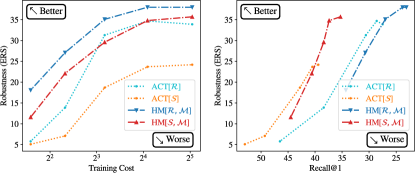
Figure 6: Performance of $\text{HM}[\mathcal{R},\mathcal{M}]$ & $\text{HM}[\mathcal{S},\mathcal{M}]$ in Tab. 3.

In contrast, HM[$\mathcal{R},\mathcal{M}$] achieves an even higher ERS under the same training cost, but with a larger penalty in R@1 compared to ACT[$\mathcal{R}$]. Compared to ACT[$\mathcal{S}$], HM[$\mathcal{S},\mathcal{M}$] is able to retain a relatively high R@1, but in a much higher efficiency. As can be seen from Fig. 6, HM[$\mathcal{R},\mathcal{M}$] achieves the highest ERS and efficiency but with the most significant drop in R@1, which is not acceptable in applications. Apart from that, HM[$\mathcal{S},\mathcal{M}$] achieves a promising result in every aspect. Its efficiency in gaining robustness is basically on par with ACT[$\mathcal{R}$], but can achieve a significantly higher R@1. It achieves a balance between ERS and R@1 on par with ACT[$\mathcal{S}$], but in a significantly higher efficiency.

			Benign Example				White-Box Attacks for Robustness Evaluation
Dataset	Defense	$\eta$	R@1$\uparrow$	R@2$\uparrow$	mAP$\uparrow$	NMI$\uparrow$	CA+$\uparrow$	CA-$\downarrow$	QA+$\uparrow$	QA-$\downarrow$	TMA$\downarrow$	ES:D$\downarrow$	ES:R$\uparrow$	LTM$\uparrow$	GTM$\uparrow$	GTT$\uparrow$	ERS$\uparrow$
	HM[$\mathcal{S},\mathcal{M}$]	8	38.4	49.7	22.9	50.3	10.9	50.5	10.8	44.6	0.680	0.722	13.3	11.2	25.8	1.2	29.6
	HM[$\mathcal{S},g_{\mathsf{B}}(\mathcal{M})$] ($\xi=0.1$)	8	36.5	48.0	21.4	48.4	13.0	44.0	13.2	35.6	0.667	0.628	20.3	13.2	26.7	2.8	33.8
	HM[$\mathcal{S},0$]	8	0.8	0.9	0.8	6.0	19.8	92.4	42.0	51.9	1.000	0.000	1.2	1.2	1.0	14.1	29.7
	HM[$\mathcal{S},-\gamma/2$]	8	36.8	47.9	21.7	48.5	12.7	41.5	12.2	35.7	0.668	0.633	18.1	14.3	28.4	2.9	33.8
	HM[$\mathcal{S},-\gamma$]	8	37.8	48.1	22.1	48.7	11.7	48.4	11.3	43.2	0.541	0.850	15.2	11.6	26.1	1.3	31.2
CUB	HM[$\mathcal{S},g_{\mathsf{LGA}}$]	8	38.0	48.3	21.8	49.3	12.7	46.4	11.6	39.9	0.567	0.783	16.8	11.9	27.9	1.4	32.4
CUB	HM[$\mathcal{S},-\gamma/2$]	2	44.5	55.9	27.6	53.3	2.4	86.1	1.3	87.7	0.809	1.091	1.5	1.8	22.1	0.1	12.4
	HM[$\mathcal{S},-\gamma/2$]	4	40.0	50.7	23.8	50.3	8.0	59.8	7.5	55.5	0.694	0.860	10.2	6.5	26.2	0.4	24.7
	HM[$\mathcal{S},-\gamma/2$]	8	36.8	47.9	21.7	48.5	12.7	41.5	12.2	35.7	0.668	0.633	18.1	14.3	28.4	2.9	33.8
	HM[$\mathcal{S},-\gamma/2$]	16	35.2	45.8	20.3	47.6	15.0	36.3	15.1	30.7	0.638	0.595	19.6	16.8	28.7	3.5	36.8
	HM[$\mathcal{S},-\gamma/2$]	32	34.7	45.5	20.0	47.5	15.0	36.7	15.1	29.9	0.631	0.611	20.1	17.2	29.3	3.5	37.0
CUB	HM[$\mathcal{S},g_{\mathsf{LGA}}$]	2	47.5	59.3	30.1	55.3	1.8	88.1	1.1	88.9	0.854	1.022	2.3	0.8	21.2	0.0	11.7
	HM[$\mathcal{S},g_{\mathsf{LGA}}$]	4	42.7	53.6	26.3	52.6	6.5	67.3	4.6	65.0	0.734	0.893	6.6	5.8	23.7	0.3	20.8
	HM[$\mathcal{S},g_{\mathsf{LGA}}$]	8	38.0	48.3	21.8	49.3	12.7	46.4	11.6	39.9	0.567	0.783	16.8	11.9	27.9	1.4	32.4
	HM[$\mathcal{S},g_{\mathsf{LGA}}$]	16	37.0	47.2	21.3	48.4	13.6	42.2	13.1	35.9	0.533	0.757	16.3	15.3	27.2	2.1	34.5
	HM[$\mathcal{S},g_{\mathsf{LGA}}$]	32	36.5	46.7	21.0	48.6	14.7	39.6	15.6	34.2	0.523	0.736	16.5	15.0	26.7	2.9	35.9

Table 4: Effectiveness of gradual adversary as $H_{\mathsf{D}}$ in hardness manipulation.

			Benign Example				White-Box Attacks for Robustness Evaluation
Dataset	Defense	$\eta$	R@1$\uparrow$	R@2$\uparrow$	mAP$\uparrow$	NMI$\uparrow$	CA+$\uparrow$	CA-$\downarrow$	QA+$\uparrow$	QA-$\downarrow$	TMA$\downarrow$	ES:D$\downarrow$	ES:R$\uparrow$	LTM$\uparrow$	GTM$\uparrow$	GTT$\uparrow$	ERS$\uparrow$
	HM[$\mathcal{R},\mathcal{M}$]	8	27.0	36.0	13.2	42.5	19.4	48.0	22.2	32.0	0.535	0.867	11.6	10.4	19.3	2.9	35.1
CUB	HM[$\mathcal{R},\mathcal{M}$]&ICS	8	25.6	34.3	12.5	41.8	21.9	41.0	23.6	26.4	0.497	0.766	14.5	13.0	21.8	4.7	39.0
	HM[$\mathcal{S},\mathcal{M}$]	8	38.4	49.7	22.9	50.3	10.9	50.5	10.8	44.6	0.680	0.722	13.3	11.2	25.8	1.2	29.6
CUB	HM[$\mathcal{S},\mathcal{M}$]&ICS	8	36.9	48.9	21.6	48.8	12.4	42.9	12.5	36.6	0.850	0.446	17.0	13.9	27.2	1.9	32.3
	HM[$\mathcal{R},g_{\mathsf{LGA}}$]	8	24.8	33.9	12.2	41.6	21.4	45.0	21.7	31.3	0.452	0.846	13.2	12.0	20.9	4.6	37.3
CUB	HM[$\mathcal{R},g_{\mathsf{LGA}}$]&ICS	8	25.7	35.2	12.8	41.7	22.1	37.1	23.4	23.7	0.464	0.725	14.5	13.3	21.1	5.3	40.2
	HM[$\mathcal{S},g_{\mathsf{LGA}}$]	8	38.0	48.3	21.8	49.3	12.7	46.4	11.6	39.9	0.567	0.783	16.8	11.9	27.9	1.4	32.4
	HM[$\mathcal{S},g_{\mathsf{LGA}}$]&ICS	8	37.2	47.8	21.4	48.4	12.9	40.9	14.7	33.7	0.806	0.487	17.1	13.2	26.3	2.3	33.5
CUB	HM[$\mathcal{S},g_{\mathsf{LGA}}$]&ICS($\lambda{=}1.0$)	8	36.0	46.7	20.7	48.0	14.2	41.0	15.1	31.7	0.907	0.329	17.0	14.2	24.5	2.1	33.7
	HM[$\mathcal{S},g_{\mathsf{LGA}}$]&ICS	2	45.2	57.2	28.5	53.7	3.0	79.9	2.4	78.9	0.936	0.609	3.6	1.2	19.9	0.0	15.2
	HM[$\mathcal{S},g_{\mathsf{LGA}}$]&ICS	4	41.8	53.0	25.3	52.0	8.1	57.3	7.9	54.1	0.892	0.514	9.8	6.7	22.9	0.5	24.6
	HM[$\mathcal{S},g_{\mathsf{LGA}}$]&ICS	8	37.2	47.8	21.4	48.4	12.9	40.9	14.7	33.7	0.806	0.487	17.1	13.2	26.3	2.3	33.5
	HM[$\mathcal{S},g_{\mathsf{LGA}}$]&ICS	16	35.5	46.4	20.4	47.5	14.9	37.2	17.1	30.3	0.771	0.495	18.2	15.3	28.7	2.8	36.0
CUB	HM[$\mathcal{S},g_{\mathsf{LGA}}$]&ICS	32	34.9	45.0	19.8	47.1	15.5	37.7	16.6	30.9	0.753	0.506	17.9	16.7	27.3	2.9	36.0

Table 5: Intra-class structure loss in conjunction with hardness manipulation for adversarial training of a DML Model.

Overall, as discussed in Sec. 3.1, HM uses the same projected gradient as to directly maximize the hardness, which endows this method a high efficiency in creating strong adversarial examples at a fixed training cost. Besides, unlike ACT, HM does not rely on the attack to successfully move the embeddings to some specific locations, and hence does not suffer from low efficiency when $\eta$ is small. HM[$\mathcal{R},\mathcal{M}$] creates training batches with some Random benign examples and a large portion of Semihard adversarial examples, and hence achieve a high ERS and a relatively low R@1 because the Random sampling strategy is not selective to benign samples on which the model does not generalize well. HM[$\mathcal{S},\mathcal{M}$] creates training batches with some Semihard adversarial examples and a large portion of Softhard benign examples, and hence achieve a relatively high ERS and a high R@1 because Softhard sampling strategy is selective. Further experiments will be based on HM[$\mathcal{S},\mathcal{M}$].

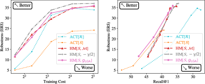
Figure 7: Performance of “HM[$\mathcal{S},g_{\mathsf{LGA}}$]” in Tab. 4.

II. Gradual Adversary. HM[$\mathcal{S},\mathcal{M}$] may still suffer from the imbalance between learning the embeddings and gaining adversarial robustness as discussed in Sec. 3.2. Hence, we conduct further experiments following the discussion, as shown in Tab. 4 and Fig. 7. Compared to HM[$\mathcal{S},\mathcal{M}$], slightly boosting the hardness with $g_{\mathsf{B}}(\cdot)$ benefits the ERS, but results in a notably lower R@1; A constant $H_{\mathsf{D}}$ at the upper bound of Semihard (i.e., $0$; too high for both the early and the late phase of training) renders model collapse; $H_{\mathsf{D}}$ at the lower bound (i.e., $-\gamma$; too low for the late phase) leads to insignificant ERS improvement; $H_{\mathsf{D}}{=}-\gamma/2$ provides a fair balance in training objectives, but still suffers from inflexibility. In contrast, being not susceptible to the mentioned problems of other choices, HM[$\mathcal{S},g_{\mathsf{LGA}}$] achieves an ERS on par with HM[$\mathcal{S},\mathcal{M}$], but is at the lowest R@1 performance penalty among all choices. Its ERS is marginally lower than HM[$\mathcal{S},{-}\gamma/2$] because the observed loss value converges around ${-}\gamma/2$ due to optimization difficulty, which means adversarial triplets with $H_{\mathsf{D}}{\in}[{-}\gamma/2,0]$ are seldom created.

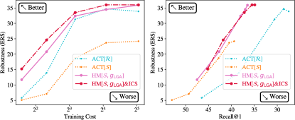
Figure 8: Performance of “HM[$\mathcal{S},g_{\mathsf{LGA}}$]&ICS” in Tab. 5.

III. Intra-Class Structure. $L_{\text{ICS}}$ is independent to HM, but is incompatible with ACT as it does not create adversarial anchor. Thus, we validate this loss term with HM. As shown in Tab. 5 and Fig. 8, $L_{\text{ICS}}$ consistently leads to a higher efficiency in gaining higher robustness at a low training cost, while retaining an acceptable trade-off in R@1.

IV. Summary. Eventually, HM[$\mathcal{S},g_{\mathsf{LGA}}$]&ICS outperforms the state-of-the-art defense in robustness, training efficiency, and R@1 performance, as shown in Fig. 1.

			Benign Example				White-Box Attacks for Robustness Evaluation
Dataset	Defense	$\eta$	R@1$\uparrow$	R@2$\uparrow$	mAP$\uparrow$	NMI$\uparrow$	CA+$\uparrow$	CA-$\downarrow$	QA+$\uparrow$	QA-$\downarrow$	TMA$\downarrow$	ES:D$\downarrow$	ES:R$\uparrow$	LTM$\uparrow$	GTM$\uparrow$	GTT$\uparrow$	ERS$\uparrow$
	N/A[$\mathcal{R}$]	N/A	53.9	66.4	26.1	59.5	0.0	100.0	0.0	99.9	0.883	1.762	0.0	0.0	14.1	0.0	3.8
	EST[$\mathcal{R}$] [53]	8	37.1	47.3	20.0	46.4	0.5	97.3	0.5	91.3	0.875	1.325	3.9	0.4	14.9	0.0	7.9
	ACT[$\mathcal{R}$] [55]	8	30.6	40.1	16.5	45.6	13.7	46.8	12.6	39.3	0.547	0.902	13.6	9.8	21.9	1.3	31.3
	HM[$\mathcal{S},g_{\mathsf{LGA}}$]	8	38.0	48.3	21.8	49.3	12.7	46.4	11.6	39.9	0.567	0.783	16.8	11.9	27.9	1.4	32.4
	HM[$\mathcal{S},g_{\mathsf{LGA}}$]&ICS	8	37.2	47.8	21.4	48.4	12.9	40.9	14.7	33.7	0.806	0.487	17.1	13.2	26.3	2.3	33.5
	EST[$\mathcal{R}$] [53]	32	8.5	13.0	2.6	25.2	2.7	97.9	0.4	97.3	0.848	1.576	1.4	0.0	4.0	0.0	5.3
	ACT[$\mathcal{R}$] [55]	32	27.5	38.2	12.2	43.0	15.5	37.7	15.1	32.2	0.472	0.821	11.1	9.4	14.9	1.0	33.9
	HM[$\mathcal{S},g_{\mathsf{LGA}}$]	32	36.5	46.7	21.0	48.6	14.7	39.6	15.6	34.2	0.523	0.736	16.5	15.0	26.7	2.9	35.9
CUB	HM[$\mathcal{S},g_{\mathsf{LGA}}$]&ICS	32	34.9	45.0	19.8	47.1	15.5	37.7	16.6	30.9	0.753	0.506	17.9	16.7	27.3	2.9	36.0
	N/A[$\mathcal{R}$]	N/A	62.5	74.0	23.8	57.0	0.2	100.0	0.1	99.6	0.874	1.816	0.0	0.0	13.4	0.0	3.6
	EST[$\mathcal{R}$] [53]	8	57.1	68.4	30.3	47.7	0.1	99.9	0.1	98.1	0.902	1.681	0.7	0.2	15.4	0.0	4.4
	ACT[$\mathcal{R}$] [55]	8	46.8	58.0	23.4	45.5	19.3	33.1	20.3	32.3	0.413	0.760	18.4	15.0	28.6	1.2	39.8
	HM[$\mathcal{S},g_{\mathsf{LGA}}$]	8	63.2	73.7	36.8	53.5	15.3	32.0	17.9	33.9	0.463	0.653	23.4	28.5	44.6	5.8	42.4
	HM[$\mathcal{S},g_{\mathsf{LGA}}$]&ICS	8	61.7	72.6	35.5	51.8	21.0	23.3	23.1	22.2	0.698	0.415	31.2	38.0	47.8	9.6	47.9
	EST[$\mathcal{R}$] [53]	32	30.7	41.0	5.6	31.8	1.2	98.1	0.4	91.8	0.880	1.281	2.9	0.7	8.2	0.0	7.3
	ACT[$\mathcal{R}$] [55]	32	43.4	54.6	11.8	42.9	18.0	32.3	17.5	30.5	0.383	0.763	16.3	15.3	20.7	1.6	38.6
	HM[$\mathcal{S},g_{\mathsf{LGA}}$]	32	62.3	72.5	35.3	52.7	17.4	28.2	18.2	28.8	0.426	0.613	27.1	30.7	42.3	7.9	44.9
CARS	HM[$\mathcal{S},g_{\mathsf{LGA}}$]&ICS	32	60.2	71.6	33.9	51.2	19.3	25.9	19.6	25.7	0.650	0.446	30.3	36.7	46.0	8.8	46.0
	N/A[$\mathcal{R}$]	N/A	62.9	68.5	39.2	87.4	0.1	99.3	0.2	99.1	0.845	1.685	0.0	0.0	6.3	0.0	4.0
	EST[$\mathcal{R}$] [53]	8	52.7	58.5	30.1	85.7	6.4	69.7	3.9	64.6	0.611	1.053	3.8	2.2	10.2	1.3	19.0
	ACT[$\mathcal{R}$] [55]	8	45.3	50.6	24.1	84.7	24.8	10.7	25.4	8.2	0.321	0.485	15.4	17.7	25.1	11.3	49.5
	HM[$\mathcal{S},g_{\mathsf{LGA}}$]	8	49.0	54.1	26.4	85.0	29.9	4.7	31.6	3.6	0.455	0.283	39.3	40.9	38.8	43.0	61.7
	HM[$\mathcal{S},g_{\mathsf{LGA}}$]&ICS	8	48.3	53.4	25.7	84.9	32.5	4.8	32.4	3.5	0.586	0.239	38.6	39.8	38.3	44.5	61.2
	EST[$\mathcal{R}$] [53]	32	46.0	51.4	24.5	84.7	12.5	43.6	10.6	34.8	0.468	0.830	9.6	7.2	17.3	3.8	31.7
	ACT[$\mathcal{R}$] [55]	32	47.5	52.6	25.5	84.9	24.1	10.5	22.7	9.4	0.253	0.532	21.2	21.6	27.8	15.3	50.8
	HM[$\mathcal{S},g_{\mathsf{LGA}}$]	32	47.7	52.7	25.3	84.8	30.6	4.7	31.2	3.5	0.466	0.266	38.6	40.3	38.6	44.3	61.8
SOP	HM[$\mathcal{S},g_{\mathsf{LGA}}$]&ICS	32	46.8	51.7	24.5	84.7	32.0	4.2	33.7	3.0	0.606	0.207	39.1	39.8	37.9	45.6	61.6

Table 6: Comparison of our defense with the state-of-the-art methods on commonly used DML datasets.

4.3 Comparison to State-of-The-Art Defense

After validating the effectiveness of our proposed method, we conduct experiments on CUB, CARS and SOP to compare our proposed method with the state-of-the-art defense methods, i.e., EST [53] and ACT [55]. The corresponding results are shown in Tab. 6. An ideal defense method should be able to achieve a high ERS and a high R@1 at a low training cost (i.e., $\eta+1$). The ability of a method to achieve a high ERS under a low training cost indicates a high efficiency.

According to the results, EST[$\mathcal{R}$] achieves a relatively high R@1 when $\eta{=}8$, but suffers from a drastic drop in R@1 when $\eta$ is increased to $32$. Nevertheless, EST[$\mathcal{R}$] only lead to a moderate robustness compared to other methods. Experiments for EST[$\mathcal{S}$] are omitted as EST has been greatly outperformed by ACT [55], and it is expected to result in even lower ERS based on the observations in previous subsections. Although ACT[$\mathcal{R}$] achieves a relatively high ERS, its R@1 performance drop is distinct on every dataset. According the previous subsections, ACT[$\mathcal{S}$] can lead to a high R@1, but along with a significantly lower ERS. Thus, results for ACT[$\mathcal{S}$] are omitted for being insufficiently robust.

Our method overwhelmingly outperforms the previous methods in terms of the overall performance. Namely, our method efficiently reaches the highest ERS with a very low decrement in R@1 under a fixed training cost. HM[$\mathcal{R},\mathcal{M}$] or HM[$\mathcal{R},g_{\mathsf{LGA}}$] can reach an even higher ERS, but are excluded from comparison due to significant drop in R@1.

It must be acknowledged that the high R@1 performance of our method largely stems from the source triplet sampling strategy, i.e., Softhard, instead of our contribution. Nevertheless, the state-of-the-art method, i.e., ACT could not reach the same level of robustness with the same sampling strategy.

It should be noted that the $L_{\text{ICS}}$ term improves robustness against most attacks involved in ERS, but also increases the tendency to collapse (observed during TMA [32] attack – high cosine similarity between two arbitrary benign examples). In some cases (e.g., on SOP), the robustness drop w.r.t TMA may neutralize the ERS gain from other attacks.

Conclusively, being selective on both benign and adversarial training samples is crucial for preventing model collapse, and achieving good performance on both types of samples. HM is a flexible tool for specifying such “selection” of adversarial examples, while LGA can be interpreted as a concrete “selection”. ICS loss further exploits the given sextuplet.

Further analysis, technical details, and limitations, etc., are presented in the supplementary document.

5 Conclusion

In this paper, HM efficiently and flexibly creates adversarial examples for adversarial training; LGA specifies an “intermediate” destination hardness for balancing robustness and performance on benign examples; ICS loss term further improves model robustness. The state-of-the-art defenses have been surpassed in terms of overall performance.

Supplementary Material

In this supplementary material, we provide more technical details and additional discussions that are excluded from the manuscript due to space limit.

Contents

1. 1 Introduction
2. 2 Related Works
3. 3 Our Approach
   1. 3.1 Hardness Manipulation
   2. 3.2 Gradual Adversary
   3. 3.3 Intra-Class Structure
4. 4 Experiments
   1. 4.1 Selection of Source & Destination Hardness
   2. 4.2 Effectiveness of Our Approach
   3. 4.3 Comparison to State-of-The-Art Defense
5. 5 Conclusion
6. A Additional Information
   1. A.1 Potential Societal Impact
   2. A.2 Limitations of Our Method
   3. A.3 Use of Existing Assets
7. B Technical Details & Minor Discussions
   1. B.1 Difference between Existing Defenses & HM
   2. B.2 Hardness Manipulation (HM)
   3. B.3 Gradual Adversary
   4. B.4 Intra-Class Structure (ICS)
   5. B.5 Experiments and Evaluation
   6. B.6 Potential Future Work

Appendix A Additional Information

A.1 Potential Societal Impact

I. Security.

Adversarial defenses alleviate the negative societal impact of adversarial attacks, and hence have positive societal impact.

A.2 Limitations of Our Method

I. Assumptions.

(1) Triplet Training Assumption.

Our method assumes sample triplets are used for training. Our method may not be compatible to other non-triplet DML loss functions. Adversarial training with other DML loss functions is left for future study.

(2) Embedding Space Assumption.

We follow the common setups [27, 55] on the embedding space. Namely, (1) the embedding vectors are normalized onto the real unit hypersphere; (2) the distance function $d(\cdot,\cdot)$ is Euclidean distance. Our formulations are developed upon the two assumptions. It is unknown whether our method method will be effective when embedding vectors are not normalized. And it is unknown whether our method will be effective when $d(\cdot,\cdot)$ is replaced as other distance metrics, e.g., cosine distance.

(3) Optimizer Assumption.

Our method assumes PGD [20] is used for optimizing the HM objective to create adversarial examples. The Eq. (4)-(5) may not necessarily hold with other possible optimizers.

II. Performance-Sensitive Factors.

(1) Maximum number of PGD iterations $\eta$.

Our method’s sensitivity to $\eta$ has been demonstrated by Tab. 3-6 and Fig. 6-8. A larger $\eta$ indicates higher training cost, and stronger adversarial examples are created for adversarial training. As a result, a larger $\eta$ leads to a higher robustness (ERS) and a lower R@1 performance. Our method consistently achieves a higher ERS under different $\eta$ settings compared to previous methods, and hence are the most efficient defense method. Experiments with $\eta$ larger than $32$ are not necessary because ERS plateaus according to Fig. 6-8.

(2) Source hardness $H_{\mathsf{S}}$ and destination hardness $H_{\mathsf{D}}$.

The $H_{\mathsf{S}}$ and $H_{\mathsf{D}}$ are the only two adjustable items in HM.

The source hardness $H_{\mathsf{S}}$ depends on triplet sampling strategy. We conduct experiments with existing triplet sampling strategies in order to focus on defense.

The choices for $H_{\mathsf{D}}$ are more flexible than those of $H_{\mathsf{S}}$, as discussed in Sec. 3.1. In the experiments, we study some possible choices following the discussion and design LGA based on the empirical observations.

(3) Parameters involved in $g_{\mathsf{LGA}}$.

Dataset	Defense	$\eta$	Benign Example				White-Box Attacks for Robustness Evaluation										ERS$\uparrow$
			R@1$\uparrow$	R@2$\uparrow$	mAP$\uparrow$	NMI$\uparrow$	CA+$\uparrow$	CA-$\downarrow$	QA+$\uparrow$	QA-$\downarrow$	TMA$\downarrow$	ES:D$\downarrow$	ES:R$\uparrow$	LTM$\uparrow$	GTM$\uparrow$	GTT$\uparrow$
CUB	HM[$\mathcal{S},g_{\mathsf{LGA}}$]	8	38.0	48.3	21.8	49.3	12.7	46.4	11.6	39.9	0.567	0.783	16.8	11.9	27.9	1.4	32.4
	HM[$\mathcal{S},g_{\mathsf{LGA}}$] ($u=2.2$)	8	34.8	45.5	15.2	47.1	13.4	36.0	17.2	26.1	0.934	0.244	20.1	15.9	27.3	3.8	36.1

Table 7: The efficacy of parameter $u$ for clipping loss value $\ell_{t-1}$. Stronger adversarial examples will be created for training if the loss value is not clipped (equivalent to setting $u$ to the theoretical upper bound of loss, i.e., 2.2).

A constant $u$ is used to normalize the loss value of the previous training iteration $\ell_{t-1}$ into $\bar{\ell}_{t-1}\in[0,1]$. The constant is empirically selected as $u=\gamma$ in our experiment. According to our observation, the loss value will quickly decrease below $\gamma$, and will remain in the $[0,\gamma]$ range for the whole training process. If we set $u$ to a larger constant than $\gamma$, the normalized loss $\bar{\ell}_{t-1}$ will be smaller, and results in stronger adversarial examples through HM[$\mathsf{S},g_{\mathsf{LGA}}$] and harms the model performance on benign examples, as shown in Tab. 7.

Another parameter in $g_{\mathsf{LGA}}$ is the triplet margin parameter $\gamma$ in order to align to the hardness range of Semihard triplets, i.e., $-\gamma<g_{\mathsf{LGA}}<0$. We follow the common setup [27] for this parameter.

(4) Constant parameter $\lambda$ for ICS loss term $L_{\text{ICS}}$.

The weight constant $\lambda$ is set as $0.5$ by default, and $0.05$ on the SOP dataset. As demonstrated in Tab. 5, there is a trade-off between robustness and performance on benign examples when tuning the $\lambda$ parameter.

Additional experiments with $\lambda=0.5$ on the SOP dataset can be found in Tab. 8. Our method is sensitive to this parameter. An excessively large $\lambda$ on the SOP datasets leads to worse performance on benign examples and worse robustness.

Dataset	Defense	$\eta$	Benign Example				White-Box Attacks for Robustness Evaluation										ERS$\uparrow$
			R@1$\uparrow$	R@2$\uparrow$	mAP$\uparrow$	NMI$\uparrow$	CA+$\uparrow$	CA-$\downarrow$	QA+$\uparrow$	QA-$\downarrow$	TMA$\downarrow$	ES:D$\downarrow$	ES:R$\uparrow$	LTM$\uparrow$	GTM$\uparrow$	GTT$\uparrow$
SOP	HM[$\mathcal{S},g_{\mathsf{LGA}}$]&ICS ($\lambda=0.5$)	8	42.4	47.1	10.2	84.2	34.9	3.8	36.7	2.3	0.879	0.093	35.3	36.5	35.2	49.1	60.1
	HM[$\mathcal{S},g_{\mathsf{LGA}}$]&ICS ($\lambda=0.5$)	32	41.5	46.1	9.9	84.1	36.1	3.1	37.6	2.1	0.873	0.086	35.7	36.8	34.7	50.2	60.8

Table 8: An excessively large $\lambda$ may lead to worse performance and robustness.

(5) Backbone deep neural network.

We adopt ResNet-18 following the state-of-the-art defense [55] for fair comparison. Since our proposed method is independent to the backbone choice, and hence is expected to be effective with different backbone models.

A.3 Use of Existing Assets

(1) Datasets.

All the datasets used in our paper are public datasets, and their corresponding papers are cited. The CUB [40] dataset includes images of birds. The CARS [14] dataset includes images of cars. The SOP [22] dataset includes images of online products.

(2) Code and Implementation.

Our implementation is built upon PyTorch and the public code of the state-of-the-art defense method ACT [55] (License: Apache-2.0).

Appendix B Technical Details & Minor Discussions

B.1 Difference between Existing Defenses & HM

I. Embedding-Shifted Triplet (EST). [53]

Embedding-Shifted Triplet (EST) [53] adopts adversarial counterparts of ${\bm{a}},{\bm{p}},{\bm{n}}$ with maximum embedding move distance off their original locations, i.e.,

$$L_{\text{EST}}=L_{\text{T}}(\tilde{{\bm{a}}},\tilde{{\bm{p}}},\tilde{{\bm{n}}};\gamma)$$ (9)

where $\tilde{{\bm{a}}}=\phi({\bm{A}}+{\bm{r}}^{*})$, and ${\bm{r}}^{*}=\arg\max_{{\bm{r}}}d_{\phi}({\bm{A}}+{\bm{r}},{\bm{A}})$. The $\tilde{{\bm{p}}}$ and $\tilde{{\bm{n}}}$ are obtained similarly.

(1) Relationship with HM:

Since EST only aims to maximize the embedding move distance off its original location without specifying any direction, it leads to a random hardness value. The expectation $E[H(\cdot)]$ of its resulting adversarial triplet is expected to be close to $E[H_{\mathsf{S}}]$. Because the perturbed triplet can be either harder or easier than the benign triplet. Namely, EST merely indirectly increase the hardness of the training triplet, and may even decrease its hardness. Thus, EST suffers from inefficiency in adversarial training compared to HM.

II. Anti-Collapse Triplet (ACT). [55]

Anti-Collapse Triplet (ACT) [55] “collapses” the embedding vectors of positive and negative sample, and enforces the model to separate them apart, i.e.,

$$L_{\text{ACT}} =L_{\text{T}}({\bm{a}},\overrightarrow{{\bm{p}}},\overleftarrow{{\bm{n}}};\gamma),$$ (10)

$$[\overrightarrow{{\bm{p}}},\overleftarrow{{\bm{n}}}] =[\phi({\bm{P}}+{\bm{r}}_{p}^{*}),\phi({\bm{N}}+{\bm{r}}_{n}^{*})]$$ (11)

$$[{\bm{r}}_{p}^{*},{\bm{r}}_{n}^{*}] =\operatorname*{arg\,min}_{{\bm{r}}_{p},{\bm{r}}_{n}}d_{\phi}({\bm{P}}+{\bm{r}}_{p},{\bm{N}}+{\bm{r}}_{n}).$$ (12)

(1) Relationship with HM:

When ACT successively “collapses” the positive and negative embedding vectors together, the hardness will be zero, i.e., $E[H(\cdot)]=0$. But ACT is not equivalent to $HM[\cdot,0]$ because the two methods have different objectives and use different gradients. Besides, in order to avoid the “misleading gradients” [55], ACT fixes the anchor and only perturb the positive and negative samples, which makes the objective for creating adversarial examples more difficult to optimize in practice. In brief, ACT is also indirectly increasing the loss value, suffering from inefficient adversarial learning.

Dataset	Defense	$\eta$	Benign Example				White-Box Attacks for Robustness Evaluation										ERS$\uparrow$
			R@1$\uparrow$	R@2$\uparrow$	mAP$\uparrow$	NMI$\uparrow$	CA+$\uparrow$	CA-$\downarrow$	QA+$\uparrow$	QA-$\downarrow$	TMA$\downarrow$	ES:D$\downarrow$	ES:R$\uparrow$	LTM$\uparrow$	GTM$\uparrow$	GTT$\uparrow$
CUB	HM[$\mathcal{S},g_{\mathsf{1/2}}$]	8	38.7	48.5	22.0	49.2	12.6	48.6	12.3	41.3	0.562	0.825	13.5	12.9	26.9	1.8	31.7
	HM[$\mathcal{S},g_{\mathsf{LGA}}$]	8	38.0	48.3	21.8	49.3	12.7	46.4	11.6	39.9	0.567	0.783	16.8	11.9	27.9	1.4	32.4
	HM[$\mathcal{S},g_{\mathsf{2}}$]	8	37.4	48.2	17.1	49.2	12.9	45.1	13.2	39.1	0.599	0.738	17.7	12.8	27.5	1.9	33.1

Table 9: Non-linear Gradual Adversary Examples.

III. Min-max Adversarial Training with Triplet Loss.

The direct formulation of min-max adversarial training [20] for triplet loss-based DML is:

$$\theta^{*}=\operatorname*{arg\,min}_{\theta}[\operatorname*{arg\,max}_{{\bm{r}}_{a},{\bm{r}}_{p},{\bm{r}}_{n}}L_{\text{T}}({\bm{A}}+{\bm{r}}_{a},{\bm{P}}+{\bm{r}}_{p},{\bm{N}}+{\bm{r}}_{n})]$$ (13)

Previous works [53, 55] point out this method will easily lead to model collapse. Our observation suggests the same.

(1) Relationship with HM:

Maximizing $L_{\text{T}}$ is equivalent to maximizing $\tilde{H}_{\mathsf{S}}$. This can be expressed as HM[$H_{\mathsf{S}},2$] as discussed in Sec. 3.1.

B.2 Hardness Manipulation (HM)

I. Adjustable Items

The only two adjustable items in HM are $H_{\mathsf{S}}$ and $H_{\mathsf{D}}$. They are discussed in the “Performance-Sensitive Factors” part of the previous section.

II. Extreme Values of Hardness.

As reflected in Sec. 3.1 and Fig. 2, the range of $H(\cdot)$ is $[-2,2]$. The embedding vectors have been normalized to the real unit hypersphere as pointed out in the manuscript. And the range of distance between any two points on the hypersphere is $[0,2]$. Hence the extreme values are:

$$\max H({\bm{A}},{\bm{P}},{\bm{N}})$$ (14)

$$= \max[d_{\phi}({\bm{A}},{\bm{P}})-d_{\phi}({\bm{A}},{\bm{N}})]$$ (15)

$$= \max[d_{\phi}({\bm{A}},{\bm{P}})]-\min[d_{\phi}({\bm{A}},{\bm{N}})]$$ (16)

$$= 2-0,$$ (17)

$$\min H({\bm{A}},{\bm{P}},{\bm{N}})$$ (18)

$$= \min[d_{\phi}({\bm{A}},{\bm{P}})-d_{\phi}({\bm{A}},{\bm{N}})]$$ (19)

$$= \min[d_{\phi}({\bm{A}},{\bm{P}})]-\max[d_{\phi}({\bm{A}},{\bm{N}})]$$ (20)

$$= 0-2.$$ (21)

Namely $H(\cdot)\in[-2,2]$. Meanwhile, since

$$L_{\text{T}}({\bm{A}},{\bm{P}},{\bm{N}};\gamma)=\max(0,H({\bm{A}},{\bm{P}},{\bm{N}})+\gamma),$$ (22)

we have $L_{\text{T}}\in[0,2+\gamma]$.

B.3 Gradual Adversary

I. Parameters

The parameters, namely $u$ and $\gamma$ are discussed in the previous section of this supplementary material, see “Performance-Sensitive Factors”.

The parameter $\xi$ in $g_{\mathsf{B}}$ is set as $0.1$, but it is not an important parameter. The function $g_{\mathsf{B}}$ is only used for demonstrating that “slightly boosting the destination hardness can further increase ERS” as discussed in Sec. 3.1.

II. Non-linear Gradual Adversary

In Sec. 3.2, more complicated designs are left for future work. We provide two Non-linear Gradual Adversary examples, namely $g_{\mathsf{2}}$ and $g_{\mathsf{1/2}}$, as follows:

$$g_{\mathsf{2}}(\cdot) =-\gamma\cdot(\bar{\ell}_{t-1})^{2} ~{}\in[-\gamma,0]$$ (23)

$$g_{\mathsf{1/2}}(\cdot) =-\gamma\cdot(\bar{\ell}_{t-1})^{1/2} ~{}\in[-\gamma,0]$$ (24)

Compared to LGA, $g_{\mathsf{2}}$ is more “eager” to result in strong adversarial examples in the early phase of training, while $g_{\mathsf{1/2}}$ is more “conservative” in creating strong adversarial examples in the early phase of training (adversarial examples from HM are stronger if the function value is closer to $0$). The corresponding experiments can be found in Tab. 9.

Dataset	Defense	$\eta$	Benign Example				White-Box Attacks for Robustness Evaluation										ERS$\uparrow$
			R@1$\uparrow$	R@2$\uparrow$	mAP$\uparrow$	NMI$\uparrow$	CA+$\uparrow$	CA-$\downarrow$	QA+$\uparrow$	QA-$\downarrow$	TMA$\downarrow$	ES:D$\downarrow$	ES:R$\uparrow$	LTM$\uparrow$	GTM$\uparrow$	GTT$\uparrow$
CUB	HM[$\mathcal{S},g_{\mathsf{LGA}}$]&ICS	8	37.2	47.8	21.4	48.4	12.9	40.9	14.7	33.7	0.806	0.487	17.1	13.2	26.3	2.3	33.5
	HM[$\mathcal{S},g_{\mathsf{LGA}}$]&$L_{\text{ICS}}(\cdots;\gamma=0.2)$	8	35.8	46.6	16.4	48.3	13.2	39.9	12.7	33.3	0.775	0.507	15.9	14.9	27.2	2.7	33.6

Table 10: The margin parameter is set to $0$ in order to avoid negative effect. R@1 performance drops with marginal robustness gain.

B.4 Intra-Class Structure (ICS)

I. Parameters

The ICS loss term can be appended to the loss for adversarial training. The only parameter for ICS loss term is the weight constant $\lambda$, and has been discussed in the “Performance-Sensitive Factors” part of the previous section.

The margin parameter is set to $0$ in order to avoid negative effect in $L_{\text{ICS}}$, as shown in Tab. 10.

II. Gradients in Fig. 5 (a) in Manuscript

According to [55], when the embedding vectors are normalized onto the real unit hypersphere and Euclidean distance is used, the gradients of the triplet loss with respect to the anchor, positive, and negative embedding vectors are respectively:

$$\frac{\partial L_{\text{T}}}{\partial{\bm{a}}} =\frac{{\bm{a}}-{\bm{p}}}{\|{\bm{a}}-{\bm{p}}\|}-\frac{{\bm{a}}-{\bm{n}}}{\|{\bm{a}}-{\bm{n}}\|}$$ (25)

$$\frac{\partial L_{\text{T}}}{\partial{\bm{p}}} =\frac{{\bm{p}}-{\bm{a}}}{\|{\bm{a}}-{\bm{p}}\|}$$ (26)

$$\frac{\partial L_{\text{T}}}{\partial{\bm{n}}} =\frac{{\bm{a}}-{\bm{n}}}{\|{\bm{a}}-{\bm{n}}\|},$$ (27)

when $L_{\text{T}}>0$. And the above equations have been reflected in Fig. 5 (a) in terms of vector direction.

III. Alternative Design for Exploiting Sextuplet

Let $\tilde{{\bm{a}}}$, $\tilde{{\bm{p}}}$, and $\tilde{{\bm{n}}}$ be $\phi({\bm{A}}+\hat{{\bm{r}}}_{a})$, $\phi({\bm{P}}+\hat{{\bm{r}}}_{p})$ and $\phi({\bm{N}}+\hat{{\bm{r}}}_{n})$ respectively. In our proposed ICS loss term, only $({\bm{a}},\tilde{{\bm{a}}},{\bm{p}})$ are involved. Other alternative selections of triplets from the sextuplet are possible, but are not as effective as $L_{\text{ICS}}$ for improving adversarial robustness.

(1) $L_{\text{T}}({\bm{a}},\tilde{{\bm{a}}},\tilde{{\bm{p}}})$

As shown in Fig. 5 (c) in the manuscript, the position of $\tilde{{\bm{p}}}$ is always further away from both ${\bm{a}}$ and $\tilde{{\bm{a}}}$ than ${\bm{p}}$ due to the gradient direction. Thus, the loss value of $L_{\text{T}}({\bm{a}},\tilde{{\bm{a}}},\tilde{{\bm{p}}})$ will always be smaller than $L_{\text{ICS}}$, and hence is less effective than $L_{\text{ICS}}$.

(2) $L_{\text{T}}({\bm{a}},{\bm{p}},{\bm{n}})$: Mixing regular training and adversarial training.

According to our observation, mixing regular training and adversarial training leads to better R@1 with drastic robustness degradation for both ACT and our defense.

(3) $L_{\text{T}}({\bm{p}},\tilde{{\bm{p}}},{\bm{a}})$: Symmetric counterpart of $L_{\text{ICS}}$.

Every sample in the training dataset will be used as anchor for once per epoch. Such symmetric loss term is duplicated to $L_{\text{ICS}}$ and is not necessary. Experimental results suggest negligible difference compared to $L_{\text{ICS}}$.

(4) $L_{\text{T}}({\bm{a}},\tilde{{\bm{a}}},\tilde{{\bm{n}}})$: $\tilde{{\bm{n}}}$ is very close to ${\bm{a}}$ in Fig. 5.

It enforces inter-class structure instead of intra-class structure. Besides, experimental results suggest negligible difference. We speculate this loss term is duplicated to the adversarial training loss term, i.e., $L_{\text{T}}(\tilde{{\bm{a}}},\tilde{{\bm{p}}},\tilde{{\bm{n}}})$, which enforces inter-class structure as well in a stronger manner.

(5) $L_{\text{T}}({\bm{a}},{\bm{p}},\tilde{{\bm{n}}})$

According to our observation, it leads to better R@1 performance on benign examples, but drastically reduce the robustness.

B.5 Experiments and Evaluation

I Hardware and Software Configuration

We conduct the experiments with two Nvidia Titan Xp GPUs (12GB of memory each) under the Ubuntu 16.04 operating system with PyTorch 1.8.2 in distributed data parallel.

II. Training Cost

In the manuscript, the training cost of adversarial training is caluclated as $\eta+1$, which is the number of forward-backward propagation involved in each iteration of the training process, in order to reflect the training efficiency (gain as high robustness as possible given a fixed number of forward-backward calculation for adversarial training) of different defense methods. Specifically, PGD creates adversarial examples from the $\eta$ times of forward-backward computation. With the resulting adversarial examples, the network requires once more forward-backward computation to update the model parameters.

III. Complete Results for Tab. 2 in Manuscript

Dataset	Defense	$\eta$	Benign Example				White-Box Attacks for Robustness Evaluation										ERS
			R@1$\uparrow$	R@2$\uparrow$	mAP$\uparrow$	NMI$\uparrow$	CA+$\uparrow$	CA-$\downarrow$	QA+$\uparrow$	QA-$\downarrow$	TMA$\downarrow$	ES:D$\downarrow$	ES:R$\uparrow$	LTM$\uparrow$	GTM$\uparrow$	GTT$\uparrow$
CUB	HM[$\mathcal{R},\mathcal{R}$]	N/A	53.9	66.4	26.1	59.5	0.0	100.0	0.0	99.9	0.883	1.762	0.0	0.0	14.1	0.0	3.8
	HM[$\mathcal{R},\mathcal{M}$]	8	27.0	36.0	13.2	42.5	19.4	48.0	22.2	32.0	0.535	0.867	11.6	10.4	19.3	2.9	35.1
	HM[$\mathcal{R},\mathcal{S}$]	8	C	o	l	l	a	p	s	e
	HM[$\mathcal{R},\mathcal{D}$]	8	C	o	l	l	a	p	s	e
	HM[$\mathcal{R},\mathcal{H}$]	8	C	o	l	l	a	p	s	e
CUB	HM[$\mathcal{M},\mathcal{R}$]	8	43.9	55.9	27.1	54.2	0.2	100.0	0.4	99.6	0.849	1.640	0.2	0.1	19.1	0.0	5.4
	HM[$\mathcal{M},\mathcal{M}$]	N/A	44.0	56.1	27.2	54.6	0.1	100.0	0.4	99.8	0.843	1.717	0.3	0.3	18.4	0.0	5.0
	HM[$\mathcal{M},\mathcal{S}$]	8	C	o	l	l	a	p	s	e
	HM[$\mathcal{M},\mathcal{D}$]	8	C	o	l	l	a	p	s	e
	HM[$\mathcal{M},\mathcal{H}$]	8	C	o	l	l	a	p	s	e
CUB	HM[$\mathcal{S},\mathcal{R}$]	8	48.3	60.1	30.3	56.3	2.0	84.4	1.4	85.4	0.835	0.895	6.1	1.6	21.0	0.0	13.7
	HM[$\mathcal{S},\mathcal{M}$]	8	38.4	49.7	22.9	50.3	10.9	50.5	10.8	44.6	0.680	0.722	13.3	11.2	25.8	1.2	29.6
	HM[$\mathcal{S},\mathcal{S}$]	N/A	55.7	68.2	35.8	61.0	0.0	100.0	0.0	99.6	0.942	1.272	0.0	0.0	19.2	0.0	6.2
	HM[$\mathcal{S},\mathcal{D}$]	8	C	o	l	l	a	p	s	e
	HM[$\mathcal{S},\mathcal{H}$]	8	C	o	l	l	a	p	s	e
CUB	HM[$\mathcal{D},\mathcal{R}$]	8	52.7	64.0	33.7	58.9	0.0	100.0	0.2	100.0	0.841	1.749	0.1	0.0	19.0	0.0	4.8
	HM[$\mathcal{D},\mathcal{M}$]	8	50.7	63.8	33.1	58.7	0.0	100.0	0.3	99.9	0.841	1.744	0.2	0.0	18.5	0.0	4.8
	HM[$\mathcal{D},\mathcal{S}$]	8	C	o	l	l	a	p	s	e
	HM[$\mathcal{D},\mathcal{D}$]	N/A	51.4	64.2	33.4	59.3	0.0	100.0	0.4	99.9	0.842	1.753	0.0	0.0	19.7	0.0	4.9
	HM[$\mathcal{D},\mathcal{H}$]	8	54.7	66.9	36.2	60.0	0.0	100.0	0.2	99.8	0.874	1.569	0.4	0.0	18.6	0.0	5.4
CUB	HM[$\mathcal{H},\mathcal{R}$]	8	51.0	63.5	32.9	59.2	0.0	100.0	0.2	99.9	0.837	1.750	0.0	0.0	17.7	0.0	4.7
	HM[$\mathcal{H},\mathcal{M}$]	8	52.2	64.0	33.1	58.4	0.0	100.0	0.2	100.0	0.841	1.750	0.0	0.0	18.9	0.0	4.8
	HM[$\mathcal{H},\mathcal{S}$]	8	C	o	l	l	a	p	s	e
	HM[$\mathcal{H},\mathcal{D}$]	8	52.6	64.9	34.4	60.0	0.0	100.0	0.2	99.9	0.835	1.720	0.1	0.0	20.0	0.0	5.1
	HM[$\mathcal{H},\mathcal{H}$]	N/A	48.9	61.2	30.3	56.5	0.0	100.0	0.4	99.9	0.830	1.752	0.2	0.0	19.5	0.0	5.0

Table 11: Full data sheet for Tab.2 in the Paper. The symbols $\mathcal{R},\mathcal{M},\mathcal{S},\mathcal{D},\mathcal{H}$ denote Random, Semihard, Softhard, Distance and Hardest triplet sampling strategies, respectively. Experiments that end up with model collapse are left with a placeholder in the table.

Complete experimental results for “Tab. 2: Combinations of Source & Destination Hardness. …” can be found in Tab. 11 of this supplementary material.

IV. Additional Notes on the Experimental Results

(1) Slight ERS decrease with a larger $\eta$

In some cases, e.g., HM[$\mathcal{S},g_{\mathsf{LGA}}$]&ICS on the CARS dataset reaches a slightly lower ERS with $\eta=32$ compared to that with $\eta=8$. We speculate this is because adversarial training suffers from overfitting [23, 26] on adversarial examples, as mentioned in Sec. 2.

B.6 Potential Future Work

I. Faster Adversarial Training with HM

As discussed in Sec. 3.1, one potential adversarial training acceleration method is to incorporate Free Adversarial Training (FAT) [29] (originally for classification) into our DML adversarial training with HM. Besides, directly incorporating FAT into the min-max adversarial training of DML will easily result in model collapse as well, because the FAT algorithm can be interpreted as to maintain a universal (agnostic to sample) perturbation that can maximize the loss. Thus, non-trivial modifications are still required to incorporate FAT FAT into adversarial training with HM. This is left for future work.

II. Better Choice for Destination Hardness

The proposed LGA function incorporates our empirical observation that “adversarial triplets should remain Semihard” based on the results in Tab. 2. However, a better choice for $H_{\mathsf{D}}$ may exist between “Semihard” and “Softhard” that can achieve better overall performance. In the manuscript, we only use the existing sampling methods and simple pseudo-hardness functions in order to avoid distraction from our focus.

III. Other Loss Functions

Adversarial trainig with DML loss functions other than triplet loss is insufficiently explored. New metric learning loss functions oriented for adversarial training are also left for future study. Besides, model collapse is an inevitable problem for adversarial training with triplet loss, and it is unknown whether other loss functions could mitigate this issue.

IV. DML & Classification

It is unknown whether DML defenses will improve the robustness in the classification task.

References

- [1] Anish Athalye, Nicholas Carlini, and David Wagner. Obfuscated gradients give a false sense of security: Circumventing defenses to adversarial examples. In Proc. Int. Conf. Mach. Learn., pages 274–283, 2018.
- [2] Qi-Zhi Cai, Chang Liu, and Dawn Song. Curriculum adversarial training. In Int. Joint Conf. Artif. Intell., page 3740–3747, 2018.
- [3] Nicholas Carlini and David Wagner. Towards evaluating the robustness of neural networks. In Proc. IEEE Symposium on Security and Privacy, pages 39–57, 2017.
- [4] Francesco Croce and Matthias Hein. Reliable evaluation of adversarial robustness with an ensemble of diverse parameter-free attacks. In Proc. Int. Conf. Mach. Learn., pages 2206–2216, 2020.
- [5] Yinpeng Dong, Qi-An Fu, Xiao Yang, Tianyu Pang, Hang Su, Zihao Xiao, and Jun Zhu. Benchmarking adversarial robustness on image classification. In Proc. IEEE Conf. Comput. Vis. Pattern Recognit., pages 321–331, 2020.
- [6] Masoud Faraki, Xiang Yu, Yi-Hsuan Tsai, Yumin Suh, and Manmohan Chandraker. Cross-domain similarity learning for face recognition in unseen domains. In Proc. IEEE Conf. Comput. Vis. Pattern Recognit., pages 15292–15301, 2021.
- [7] Yan Feng, Bin Chen, Tao Dai, and Shu-Tao Xia. Adversarial attack on deep product quantization network for image retrieval. In Proc. AAAI. Conf. Artif. Intell., pages 10786–10793, 2020.
- [8] Ian J Goodfellow, Jonathon Shlens, and Christian Szegedy. Explaining and harnessing adversarial examples. In Proc. Int. Conf. Learn. Representations, 2015.
- [9] Kaiming He, Xiangyu Zhang, Shaoqing Ren, and Jian Sun. Deep residual learning for image recognition. In Proc. IEEE Conf. Comput. Vis. Pattern Recognit., pages 770–778, 2016.
- [10] Warren He, James Wei, Xinyun Chen, Nicholas Carlini, and Dawn Song. Adversarial example defense: Ensembles of weak defenses are not strong. In USENIX Workshop on Offensive Technologies, page 15, 2017.
- [11] Hanxun Huang, Yisen Wang, Sarah Monazam Erfani, Quanquan Gu, James Bailey, and Xingjun Ma. Exploring architectural ingredients of adversarially robust deep neural networks. In Proc. Conf. Neural Inf. Process. Syst., 2021.
- [12] Andrew Ilyas, Logan Engstrom, Anish Athalye, and Jessy Lin. Black-box adversarial attacks with limited queries and information. In Proc. Int. Conf. Mach. Learn., pages 2137–2146, 2018.
- [13] Diederik P. Kingma and Jimmy Ba. Adam: A method for stochastic optimization. In Proc. Int. Conf. Learn. Representations, 2015.
- [14] Jonathan Krause, Michael Stark, Jia Deng, and Li Fei-Fei. 3d object representations for fine-grained categorization. In Proc. Int. Conf. Comput. Vis. Workshops, pages 554–561, 2013.
- [15] Alexey Kurakin, Ian Goodfellow, and Samy Bengio. Adversarial examples in the physical world. In Proc. Int. Conf. Learn. Representations Workshops, 2017.
- [16] Jie Li, Rongrong Ji, Hong Liu, Xiaopeng Hong, Yue Gao, and Qi Tian. Universal perturbation attack against image retrieval. In Proc. Int. Conf. Comput. Vis., pages 4899–4908, 2019.
- [17] Xiaodan Li, Jinfeng Li, Yuefeng Chen, Shaokai Ye, Yuan He, Shuhui Wang, Hang Su, and Hui Xue. Qair: Practical query-efficient black-box attacks for image retrieval. In Proc. IEEE Conf. Comput. Vis. Pattern Recognit., 2021.
- [18] Wei-An Lin, Chun Pong Lau, Alexander Levine, Rama Chellappa, and Soheil Feizi. Dual manifold adversarial robustness: Defense against lp and non-lp adversarial attacks. arXiv preprint arXiv:2009.02470, 2020.
- [19] Xuanqing Liu, Minhao Cheng, Huan Zhang, and Cho-Jui Hsieh. Towards robust neural networks via random self-ensemble. In Proc. Eur. Conf. Comput. Vis., pages 369–385, 2018.
- [20] Aleksander Madry, Aleksandar Makelov, Ludwig Schmidt, Dimitris Tsipras, and Adrian Vladu. Towards deep learning models resistant to adversarial attacks. In Proc. Int. Conf. Learn. Representations, 2018.
- [21] Kevin Musgrave, Serge Belongie, and Ser-Nam Lim. A metric learning reality check. In Proc. Eur. Conf. Comput. Vis., pages 681–699, 2020.
- [22] Hyun Oh Song, Yu Xiang, Stefanie Jegelka, and Silvio Savarese. Deep metric learning via lifted structured feature embedding. In Proc. IEEE Conf. Comput. Vis. Pattern Recognit., pages 4004–4012, 2016.
- [23] Tianyu Pang, Xiao Yang, Yinpeng Dong, Hang Su, and Jun Zhu. Bag of tricks for adversarial training. In Proc. Int. Conf. Learn. Representations, 2021.
- [24] Nicolas Papernot, Patrick McDaniel, Xi Wu, Somesh Jha, and Ananthram Swami. Distillation as a defense to adversarial perturbations against deep neural networks. In Proc. IEEE Symposium on Security and Privacy, pages 582–597, 2016.
- [25] Aaditya Prakash, Nick Moran, Solomon Garber, Antonella DiLillo, and James Storer. Deflecting adversarial attacks with pixel deflection. In Proc. IEEE Conf. Comput. Vis. Pattern Recognit., pages 8571–8580, 2018.
- [26] Leslie Rice, Eric Wong, and Zico Kolter. Overfitting in adversarially robust deep learning. In Proc. Int. Conf. Mach. Learn., pages 8093–8104, 2020.
- [27] Karsten Roth, Timo Milbich, Samarth Sinha, Prateek Gupta, Bjorn Ommer, and Joseph Paul Cohen. Revisiting training strategies and generalization performance in deep metric learning. In Proc. Int. Conf. Mach. Learn., pages 8242–8252, 2020.
- [28] Florian Schroff, Dmitry Kalenichenko, and James Philbin. Facenet: A unified embedding for face recognition and clustering. In Proc. IEEE Conf. Comput. Vis. Pattern Recognit., pages 815–823, 2015.
- [29] Ali Shafahi, Mahyar Najibi, Mohammad Amin Ghiasi, Zheng Xu, John Dickerson, Christoph Studer, Larry S Davis, Gavin Taylor, and Tom Goldstein. Adversarial training for free! In Proc. Conf. Neural Inf. Process. Syst., 2019.
- [30] Chawin Sitawarin, Supriyo Chakraborty, and David Wagner. Sat: Improving adversarial training via curriculum-based loss smoothing. In Proc. of the 14th ACM Workshop on Artificial Intelligence and Security, page 25–36, 2021.
- [31] Christian Szegedy, Wojciech Zaremba, Ilya Sutskever, Joan Bruna, Dumitru Erhan, Ian Goodfellow, and Rob Fergus. Intriguing properties of neural networks. In Proc. Int. Conf. Learn. Representations, 2014.
- [32] Giorgos Tolias, Filip Radenovic, and Ondrej Chum. Targeted mismatch adversarial attack: Query with a flower to retrieve the tower. In Proc. Int. Conf. Comput. Vis., pages 5037–5046, 2019.
- [33] Florian Tramer, Nicholas Carlini, Wieland Brendel, and Aleksander Madry. On adaptive attacks to adversarial example defenses. In Proc. Conf. Neural Inf. Process. Syst., pages 1633–1645, 2020.
- [34] Dimitris Tsipras, Shibani Santurkar, Logan Engstrom, Alexander Turner, and Aleksander Madry. Robustness may be at odds with accuracy. In Proc. Int. Conf. Learn. Representations, 2019.
- [35] Jonathan Uesato, Brendan O’donoghue, Pushmeet Kohli, and Aaron Oord. Adversarial risk and the dangers of evaluating against weak attacks. In Proc. Int. Conf. Mach. Learn., pages 5025–5034, 2018.
- [36] Hongjun Wang, Guangrun Wang, Ya Li, Dongyu Zhang, and Liang Lin. Transferable, controllable, and inconspicuous adversarial attacks on person re-identification with deep mis-ranking. In Proc. IEEE Conf. Comput. Vis. Pattern Recognit., pages 342–351, 2020.
- [37] Jiang Wang, Yang Song, Thomas Leung, Chuck Rosenberg, Jingbin Wang, James Philbin, Bo Chen, and Ying Wu. Learning fine-grained image similarity with deep ranking. In Proc. IEEE Conf. Comput. Vis. Pattern Recognit., pages 1386–1393, 2014.
- [38] Jianyu Wang and Haichao Zhang. Bilateral adversarial training: Towards fast training of more robust models against adversarial attacks. In Proc. Int. Conf. Comput. Vis., pages 6629–6638, 2019.
- [39] Zhibo Wang, Siyan Zheng, Mengkai Song, Qian Wang, Alireza Rahimpour, and Hairong Qi. Advpattern: Physical-world attacks on deep person re-identification via adversarially transformable patterns. In Proc. Int. Conf. Comput. Vis., pages 8341–8350, 2019.
- [40] P. Welinder, S. Branson, T. Mita, C. Wah, F. Schroff, S. Belongie, and P. Perona. Caltech-ucsd birds 200. Technical Report CNS-TR-2010-001, California Institute of Technology, 2010.
- [41] Eric Wong, Leslie Rice, and J. Zico Kolter. Fast is better than free: Revisiting adversarial training. In Proc. Int. Conf. Learn. Representations, 2020.
- [42] Chao-Yuan Wu, R. Manmatha, Alexander J. Smola, and Philipp Krahenbuhl. Sampling matters in deep embedding learning. In Proc. Int. Conf. Comput. Vis., pages 2840–2848, 2017.
- [43] Dongxian Wu, Shu-Tao Xia, and Yisen Wang. Adversarial weight perturbation helps robust generalization. In Proc. Conf. Neural Inf. Process. Syst., 2020.
- [44] Dongxian Wu, Shu-Tao Xia, and Yisen Wang. Adversarial weight perturbation helps robust generalization. In Proc. Conf. Neural Inf. Process. Syst., 2020.
- [45] Cihang Xie, Zhishuai Zhang, Yuyin Zhou, Song Bai, Jianyu Wang, Zhou Ren, and Alan L Yuille. Improving transferability of adversarial examples with input diversity. In Proc. IEEE Conf. Comput. Vis. Pattern Recognit., pages 2730–2739, 2019.
- [46] Yunrui Yu, Xitong Gao, and Cheng-Zhong Xu. Lafeat: Piercing through adversarial defenses with latent features. In Proc. IEEE Conf. Comput. Vis. Pattern Recognit., pages 5735–5745, 2021.
- [47] Dinghuai Zhang, Tianyuan Zhang, Yiping Lu, Zhanxing Zhu, and Bin Dong. You only propagate once: Accelerating adversarial training via maximal principle. In Proc. Conf. Neural Inf. Process. Syst., pages 227–238, 2019.
- [48] Haichao Zhang and Jianyu Wang. Defense against adversarial attacks using feature scattering-based adversarial training. In Proc. Conf. Neural Inf. Process. Syst., 2019.
- [49] Hongyang Zhang, Yaodong Yu, Jiantao Jiao, Eric Xing, Laurent El Ghaoui, and Michael Jordan. Theoretically principled trade-off between robustness and accuracy. In Proc. Int. Conf. Mach. Learn., pages 7472–7482, 2019.
- [50] Jingfeng Zhang, Jianing Zhu, Gang Niu, Bo Han, Masashi Sugiyama, and Mohan Kankanhalli. Geometry-aware instance-reweighted adversarial training. In Proc. Int. Conf. Learn. Representations, 2021.
- [51] Yaoyao Zhong and Weihong Deng. Adversarial learning with margin-based triplet embedding regularization. In Proc. Int. Conf. Comput. Vis., pages 6549–6558, 2019.
- [52] Mo Zhou, Zhenxing Niu, Le Wang, Zhanning Gao, Qilin Zhang, and Gang Hua. Ladder loss for coherent visual-semantic embedding. In Proc. AAAI. Conf. Artif. Intell., pages 13050–13057, 2020.
- [53] Mo Zhou, Zhenxing Niu, Le Wang, Qilin Zhang, and Gang Hua. Adversarial ranking attack and defense. In Proc. Eur. Conf. Comput. Vis., pages 781–799, 2020.
- [54] Mo Zhou, Le Wang, Zhenxing Niu, Qilin Zhang, Yinghui Xu, Nanning Zheng, and Gang Hua. Practical relative order attack in deep ranking. In Proc. Int. Conf. Comput. Vis., 2021.
- [55] Mo Zhou, Le Wang, Zhenxing Niu, Qilin Zhang, Nanning Zheng, and Gang Hua. Adversarial attack and defense in deep ranking. In arXiv preprint 2106.03614, 2021.