MUAD: Multiple Uncertainties for Autonomous Driving, a benchmark for multiple uncertainty types and tasks

Abstract

Predictive uncertainty estimation is essential for safe deployment of Deep Neural Networks in real-world autonomous systems. However, disentangling the different types and sources of uncertainty is non trivial for most datasets, especially since there is no ground truth for uncertainty. In addition, while adverse weather conditions of varying intensities can disrupt neural network predictions, they are usually under-represented in both training and test sets in public datasets. We attempt to mitigate these setbacks and introduce the MUAD dataset (Multiple Uncertainties for Autonomous Driving), consisting of 10,413 realistic synthetic images with diverse adverse weather conditions (night, fog, rain, snow), out-of-distribution objects and annotations for semantic segmentation, depth estimation, object and instance detection. MUAD allows to better assess the impact of different sources of uncertainty on model performance. We conduct a thorough experimental study of this impact on several baseline Deep Neural Networks across multiple tasks, and release our dataset to allow researchers to benchmark their algorithm methodically in adverse conditions. More visualizations and the download link for MUAD are available at https://muad-dataset.github.io/.

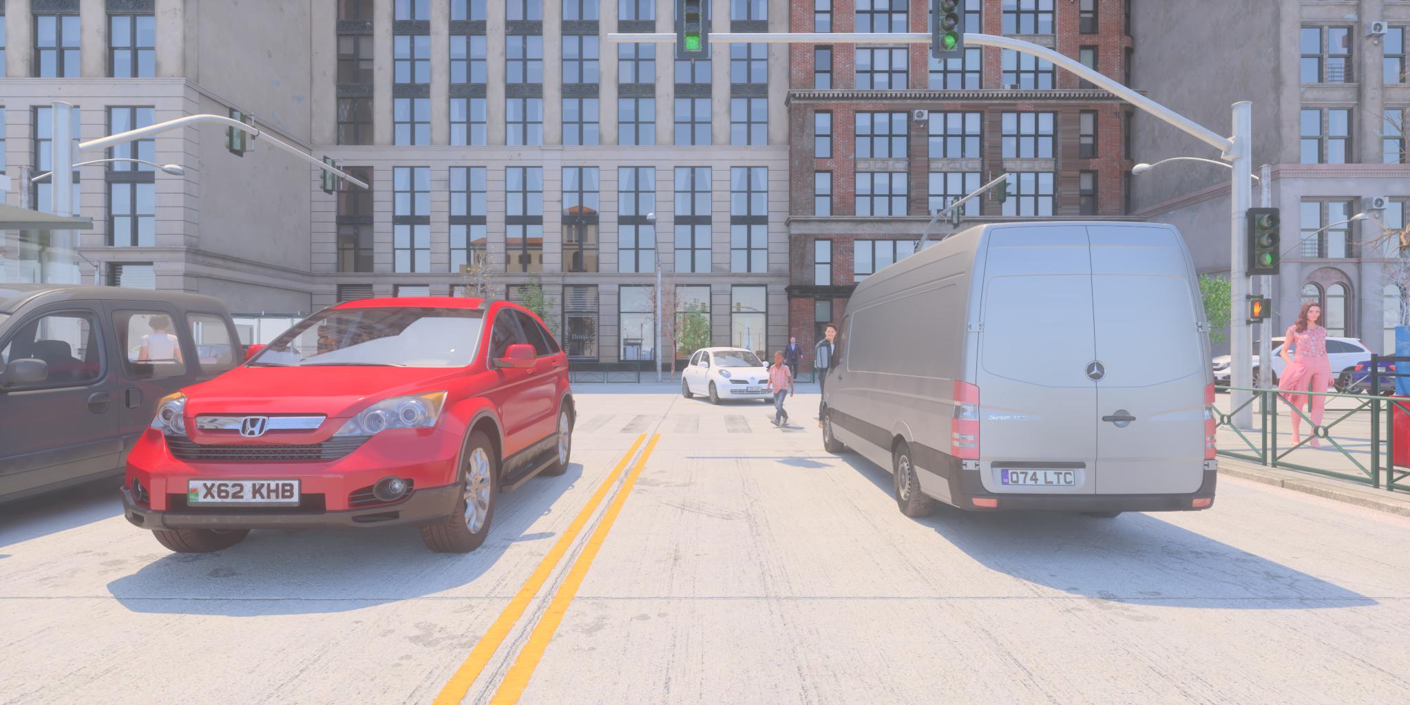
(a) No perturbation

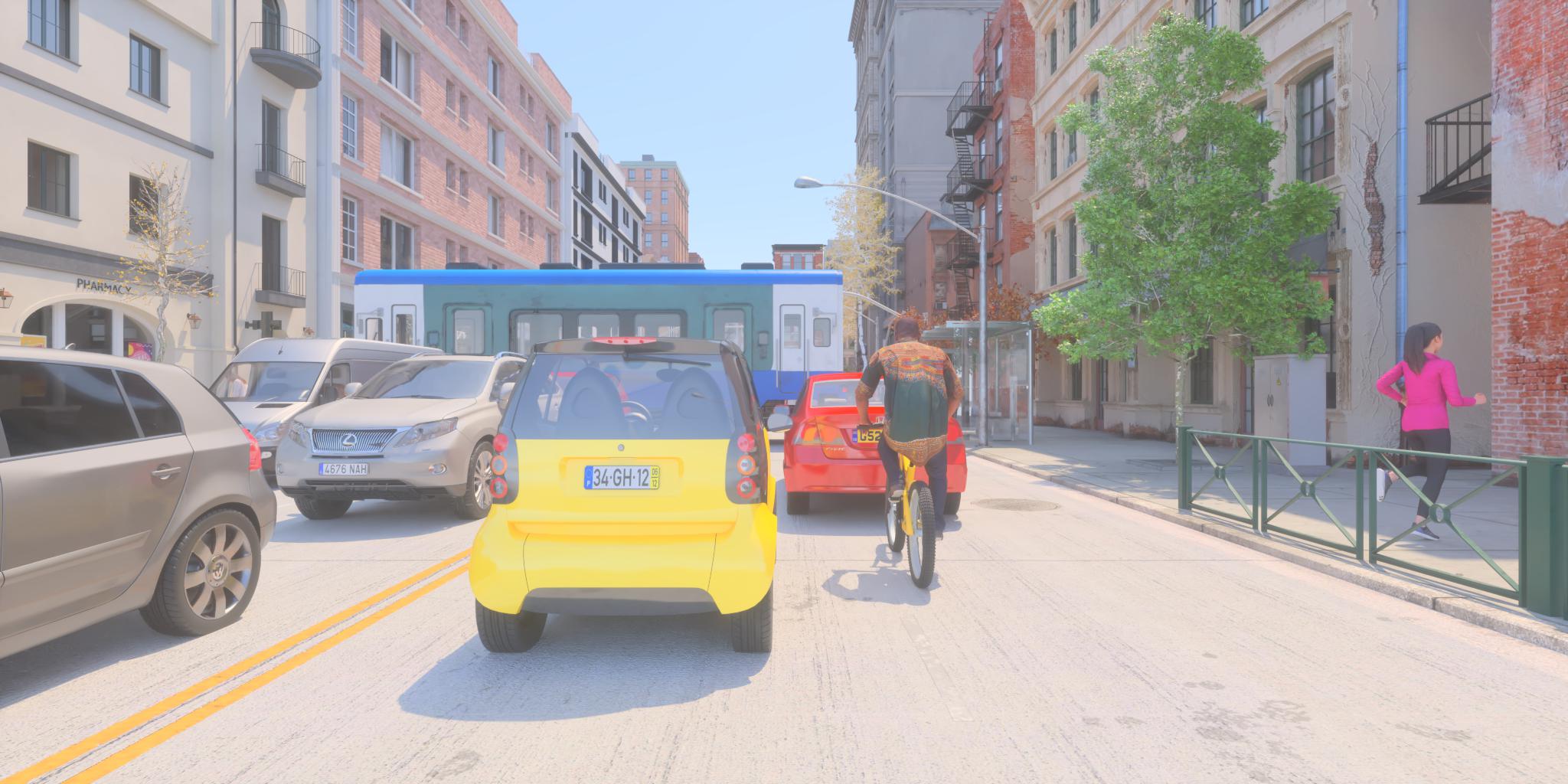
(b) With OOD instances

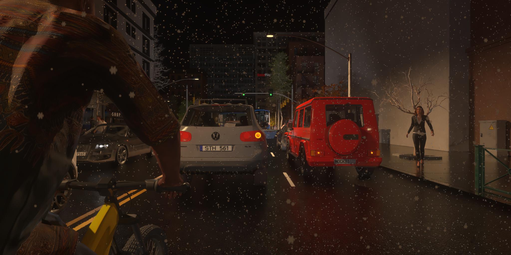
(c) Level 1 perturbation

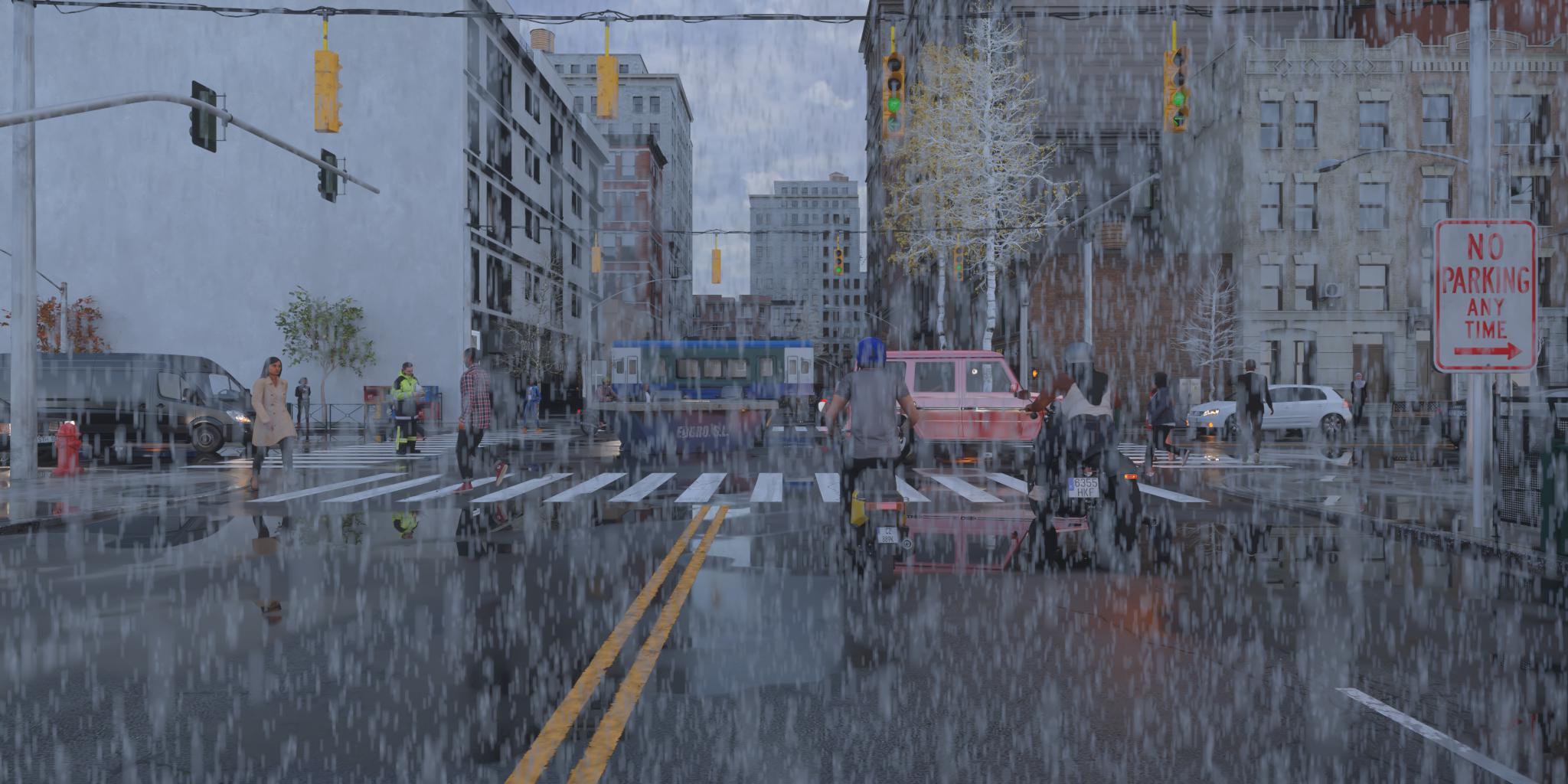
(d) Level 2 perturbation

Figure 1: Snapshots from the MUAD dataset showing different types of adverse conditions and events to evaluate perception models (OOD : Out Of Distribution, i.e., not seen during training).

1 Introduction

In recent years, Deep Neural Networks (DNNs) have achieved remarkable results in various computer vision tasks [Krizhevsky et al.(2012)Krizhevsky, Sutskever, and Hinton, Ren et al.(2015b)Ren, He, Girshick, and Sun, Chen et al.(2017a)Chen, Papandreou, Kokkinos, Murphy, and Yuille]. This has turned DNNs into an essential tool for effective automatic perception. Although DNNs achieve outstanding performance across benchmarks and tasks, there are still a few major bottlenecks to solve before a widespread deployment. One of the most frequent and known criticisms of DNNs is related to their lack of reliability under varying levels of shifts in the data distribution, and it became crucial to address this limitation. To achieve this, we focus on studying the uncertainties of the DNN predictions for computer vision tasks. The predictive uncertainty of a DNN stems from two main types of uncertainty [Hora(1996)]: aleatoric and epistemic. The former is related to randomness of the world and of the sensing system, typically instantiated as noise in the data. The latter concerns finite size training datasets. The epistemic uncertainty captures the uncertainty in the DNN parameters and their lack of knowledge on the model that generated the training data. In spite of their simple and intuitive definitions, the sources of uncertainty are notoriously hard to separate in most datasets, where data are typically curated and various outlier or noisy samples are removed before annotation.

For autonomous driving, uncertainty estimation and reliability are essential for safely deploying DNNs in real-world conditions. Here, DNNs are expected not only to reach high predictive performance and real-time inference speed, but also to deal effectively with the two types of uncertainty under various forms (noise, distribution shift, out-of-distribution samples, sensor degradation, etc.). In the last years, numerous works have moved the needle towards more reliable predictive uncertainty for DNNs [Blundell et al.(2015)Blundell, Cornebise, Kavukcuoglu, and Wierstra, Gal and Ghahramani(2016), Lakshminarayanan et al.(2017)Lakshminarayanan, Pritzel, and Blundell, Kendall and Gal(2017), Wen et al.(2020)Wen, Tran, and Ba, Franchi et al.(2020a)Franchi, Bursuc, Aldea, Dubuisson, and Bloch, Mukhoti et al.(2020)Mukhoti, Kulharia, Sanyal, Golodetz, Torr, and Dokania, Besnier et al.(2021)Besnier, Bursuc, Picard, and Briot, Mukhoti et al.(2021)Mukhoti, Kirsch, van Amersfoort, Torr, and Gal]. However, evaluating such methods is not obvious as there is no ground truth for uncertainty and the different sources of uncertainty are conflated due to prior data curation.

We introduce a new dataset to study uncertainty estimation methods for perception in autonomous vehicles. While most datasets aim to improve the predictive performance of DNNs [Geiger et al.(2012)Geiger, Lenz, and Urtasun, Cordts et al.(2016)Cordts, Omran, Ramos, Rehfeld, Enzweiler, Benenson, Franke, Roth, and Schiele, Neuhold et al.(2017)Neuhold, Ollmann, Rota Bulo, and Kontschieder, Yu et al.(2020)Yu, Chen, Wang, Xian, Chen, Liu, Madhavan, and Darrell], only recently datasets addressed the robustness of DNNs under unseen weather conditions [Sakaridis et al.(2020)Sakaridis, Dai, and Van Gool, Dai et al.(2020)Dai, Sakaridis, Hecker, and Van Gool, Sakaridis et al.(2021)Sakaridis, Dai, and Van Gool] or objects [Hendrycks et al.(2019)Hendrycks, Basart, Mazeika, Mostajabi, Steinhardt, and Song, Blum et al.(2019)Blum, Sarlin, Nieto, Siegwart, and Cadena, Chan et al.(2021)Chan, Lis, Uhlemeyer, Blum, Honari, Siegwart, Salzmann, Fua, and Rottmann]. However, these datasets are either limited to only one task, typically semantic segmentation, or only focus on a single type of uncertainty, or are not being precise enough in the different levels of uncertainties. We address these limitations in our dataset that allows to quantify all levels of uncertainty in the same conditions. Our dataset, MUAD (Multiple Uncertainties for Autonomous Driving) is composed of 3,420 images for training, 492 for validation, and 6,501 for testing.

To summarize, our contributions are as follows: (1) We introduce MUAD: a new automotive dataset with annotations for multiple tasks and multiple uncertainty sources. (2) We perform a wide range of benchmarks on MUAD dataset for multiple computer vision tasks and settings (semantic segmentation, depth estimation, object detection) to further support research in this area. (3) We conduct an extensive study on uncertainty quantification for 2D output tasks for recent Transformer-based architectures.

2 Related work

2.1 Datasets

A variety of real-world datasets for autonomous driving have been recently released [Cordts et al.(2016)Cordts, Omran, Ramos, Rehfeld, Enzweiler, Benenson, Franke, Roth, and Schiele, Geiger et al.(2012)Geiger, Lenz, and Urtasun, Sun et al.(2020)Sun, Kretzschmar, Dotiwalla, Chouard, Patnaik, Tsui, Guo, Zhou, Chai, Caine, Vasudevan, Han, Ngiam, Zhao, Timofeev, Ettinger, Krivokon, Gao, Joshi, Zhang, Shlens, Chen, and Anguelov, Caesar et al.(2020)Caesar, Bankiti, Lang, Vora, Liong, Xu, Krishnan, Pan, Baldan, and Beijbom, Yu et al.(2020)Yu, Chen, Wang, Xian, Chen, Liu, Madhavan, and Darrell, Varma et al.(2019)Varma, Subramanian, Namboodiri, Chandraker, and Jawahar, Ramanishka et al.(2018)Ramanishka, Chen, Misu, and Saenko, Chang et al.(2019)Chang, Lambert, Sangkloy, Singh, Bak, Hartnett, Wang, Carr, Lucey, Ramanan, et al., Houston et al.(2020)Houston, Zuidhof, Bergamini, Ye, Chen, Jain, Omari, Iglovikov, and Ondruska]. They have enabled tremendous progress in the area but they typically focus on a single task, e.g., semantic segmentation [Cordts et al.(2016)Cordts, Omran, Ramos, Rehfeld, Enzweiler, Benenson, Franke, Roth, and Schiele, Yu et al.(2020)Yu, Chen, Wang, Xian, Chen, Liu, Madhavan, and Darrell, Ramanishka et al.(2018)Ramanishka, Chen, Misu, and Saenko], object detection [Geiger et al.(2012)Geiger, Lenz, and Urtasun, Sun et al.(2020)Sun, Kretzschmar, Dotiwalla, Chouard, Patnaik, Tsui, Guo, Zhou, Chai, Caine, Vasudevan, Han, Ngiam, Zhao, Timofeev, Ettinger, Krivokon, Gao, Joshi, Zhang, Shlens, Chen, and Anguelov, Caesar et al.(2020)Caesar, Bankiti, Lang, Vora, Liong, Xu, Krishnan, Pan, Baldan, and Beijbom], motion prediction [Chang et al.(2019)Chang, Lambert, Sangkloy, Singh, Bak, Hartnett, Wang, Carr, Lucey, Ramanan, et al., Houston et al.(2020)Houston, Zuidhof, Bergamini, Ye, Chen, Jain, Omari, Iglovikov, and Ondruska] and do not have evaluation tracks for uncertainty and out-of-distribution detection. Synthetic datasets, e.g., GTA-V [Richter et al.(2016)Richter, Vineet, Roth, and Koltun], SYNTHIA [Ros et al.(2016)Ros, Sellart, Materzynska, Vazquez, and Lopez], virtual KITTI [Gaidon et al.(2016)Gaidon, Wang, Cabon, and Vig] can provide abundant training data alleviating the need for costly annotation of real images as well as privacy preservation concerns in the case of real data. Currently, they are mostly designed and used for domain adaptation, typically imitating the content and classes from a given real dataset. Several datasets have emerged towards meeting the reliability requirement for self-driving vehicles [Blum et al.(2019)Blum, Sarlin, Nieto, Siegwart, and Cadena, Pinggera et al.(2016)Pinggera, Ramos, Gehrig, Franke, Rother, and Mester, Chan et al.(2021)Chan, Lis, Uhlemeyer, Blum, Honari, Siegwart, Salzmann, Fua, and Rottmann, Hendrycks et al.(2019)Hendrycks, Basart, Mazeika, Mostajabi, Steinhardt, and Song] and evaluate the performance of semantic segmentation DNNs when facing out-of-distribution objects (OOD). Other datasets investigate the robustness against different weather conditions, e.g., night [Dai et al.(2020)Dai, Sakaridis, Hecker, and Van Gool, Dai and Van Gool(2018), Sakaridis et al.(2021)Sakaridis, Dai, and Van Gool], rain [Tung et al.(2017)Tung, Chen, Meng, and Little, Sakaridis et al.(2021)Sakaridis, Dai, and Van Gool], fog [Sakaridis et al.(2018)Sakaridis, Dai, and Van Gool, Sakaridis et al.(2021)Sakaridis, Dai, and Van Gool], however they are often acquired in different locations and conditions leading to a performance drop that overlaps with the one from the difficult weather conditions.

In order to provide images of the same locations, to address the lack of diversity in real environments and to evaluate better the impact on the epistemic uncertainty, some works promoted inpainting of virtual objects [Hendrycks et al.(2019)Hendrycks, Basart, Mazeika, Mostajabi, Steinhardt, and Song] or synthesised weather conditions [Tremblay et al.(2021)Tremblay, Halder, de Charette, and Lalonde]. In this setting however, questions may be raised about the veracity of the result. Therefore, the recent ACDC dataset [Sakaridis et al.(2021)Sakaridis, Dai, and Van Gool] is composed entirely of real images taken from the same locations, and includes multiple sources of aleatoric uncertainty. However, not having any control on the noise level makes it harder to quantify the link between noise and uncertainty. Acquiring images with uncertainty corner cases is problematic as these cases are rare (long tail) and also costly to annotate, e.g., 3.3 hours/image [Sakaridis et al.(2021)Sakaridis, Dai, and Van Gool]. Given this scarcity, such images are better used for validation as a small test set to assess the reliability of DNNs before deployment. These system validation stages can be seen as stress tests with corner cases to mirror challenging real-world conditions. It is thus interesting even from a more applied standpoint to have a synthetic dataset that mimics these rare conditions with some good fidelity constraint to quantify the robustness of DNNs. Synthetic data is abundant and can allow us to measure finer drifts in the input distribution. In addition, most such datasets mainly focus on semantic segmentation, while we propose to address multiple tasks (semantic segmentation, monocular depth, object detection, and instance segmentation).

In Table 1 we provide a summary of the main existing uncertainty datasets. In this work, we propose a fully synthetic dataset, called MUAD, integrating different weather conditions with various intensities, and suitable for a multitude of vision tasks and for the comprehensive characterisation of their uncertainty.

Dataset	Adversarial annotations	Fog	Night	Rain	Snow	Classes	Out of distribution	Depth	Object detection 2D/3D	Instance segmentation
Foggy Driving[Sakaridis et al.(2018)Sakaridis, Dai, and Van Gool]	101	✓	-	-	-	19	-	-	✓	-
Foggy Zurich [Dai et al.(2020)Dai, Sakaridis, Hecker, and Van Gool]	40	✓	-	-	-	19	-	-	-	-
Nighttime Driving [Dai and Van Gool(2018)]	50	-	✓	-	-	19	-	-	-	-
Dark Zurich [Sakaridis et al.(2020)Sakaridis, Dai, and Van Gool]	201	-	✓	-	-	19	-	-	-	-
Raincouver [Tung et al.(2017)Tung, Chen, Meng, and Little]	326	-	✓	✓	-	3	-	-	-	-
WildDash [Zendel et al.(2018)Zendel, Honauer, Murschitz, Steininger, and Dominguez]	226	✓	✓	✓	✓	19	-	-	-	-
BDD100K [Yu et al.(2020)Yu, Chen, Wang, Xian, Chen, Liu, Madhavan, and Darrell]	1346	✓	✓	✓	✓	19	-	-	-	-
ACDC [Sakaridis et al.(2021)Sakaridis, Dai, and Van Gool]	4006	✓	✓	✓	✓	19	-	✓	✓	-
Virtual KITTI 2 [Cabon et al.(2020)Cabon, Murray, and Humenberger]	21260	✓	-	✓	-	14	-	✓	✓	✓
Fishyscapes [Blum et al.(2019)Blum, Sarlin, Nieto, Siegwart, and Cadena]	373	-	-	-	-	19+2	✓	-	-	-
LostAndFound [Pinggera et al.(2016)Pinggera, Ramos, Gehrig, Franke, Rother, and Mester]	1203	-	-	-	-	19+9	✓	-	-	-
RoadObstacle21 [Chan et al.(2021)Chan, Lis, Uhlemeyer, Blum, Honari, Siegwart, Salzmann, Fua, and Rottmann]	327	-	✓	-	✓	19+1	✓	-	-	-
RoadAnomaly21 [Chan et al.(2021)Chan, Lis, Uhlemeyer, Blum, Honari, Siegwart, Salzmann, Fua, and Rottmann]	100	-	-	-	✓	19+1	✓	-	-	-
Streethazard [Hendrycks et al.(2019)Hendrycks, Basart, Mazeika, Mostajabi, Steinhardt, and Song]	6625	-	-	-	-	13+250	✓	-	-	-
BDD anomaly [Hendrycks et al.(2019)Hendrycks, Basart, Mazeika, Mostajabi, Steinhardt, and Song]	810	✓	✓	✓	✓	17+2	✓	-	-	-
MUAD	10413	✓	✓	✓	✓	16+9	✓	✓	✓	✓

Table 1: Comparative overview of the different datasets for uncertainty on autonomous driving.

2.2 Uncertainty

Several works address the two types of uncertainty, in particular for the classification task. Most approaches build upon Bayesian learning, frequently using Bayesian Neural Networks (BNNs) [Blundell et al.(2015)Blundell, Cornebise, Kavukcuoglu, and Wierstra, Hernández-Lobato and Adams(2015), Maddox et al.(2019)Maddox, Izmailov, Garipov, Vetrov, and Wilson, Franchi et al.(2020b)Franchi, Bursuc, Aldea, Dubuisson, and Bloch, Wilson and Izmailov(2020), Dusenberry et al.(2020)Dusenberry, Jerfel, Wen, Ma, Snoek, Heller, Lakshminarayanan, and Tran, Franchi et al.(2020a)Franchi, Bursuc, Aldea, Dubuisson, and Bloch], which estimate the posterior distribution of the DNN weights to marginalize the likelihood distribution at inference time. Yet most BNNs are difficult to train and scale to complex computer vision tasks that have been addressed, so far, by fewer uncertainty estimation methods. Ensembles [Lakshminarayanan et al.(2017)Lakshminarayanan, Pritzel, and Blundell] and pseudo-ensembles [Gal and Ghahramani(2016), Maddox et al.(2019)Maddox, Izmailov, Garipov, Vetrov, and Wilson, Franchi et al.(2020b)Franchi, Bursuc, Aldea, Dubuisson, and Bloch] achieve state-of-the-art performance on various tasks, at the high cost of multiple training and/or multiple forward passes at inference. Some approaches [Kendall and Gal(2017)] formalize DNNs to output a parametric distribution, and their goal is to estimate the distribution parameters. These approaches can be applied to optical flow [Ilg et al.(2018)Ilg, Cicek, Galesso, Klein, Makansi, Hutter, and Brox] and object detection [Choi et al.(2019)Choi, Chun, Kim, and Lee], yet they mainly focus on aleatoric uncertainty. Besides the additional challenges posed by complex computer vision tasks, progress on uncertainty estimation in this area is hindered by the lower number of datasets for properly assessing both the quality of the predictive uncertainty and the predictive performance. With MUAD we hope to encourage research in this essential area for practical applications with annotations and benchmarks for multiple tasks.

3 Multiple Uncertainties for Autonomous Driving benchmark (MUAD)

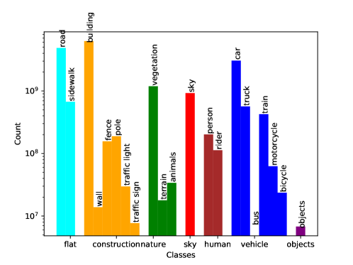
Figure 2: Number of annotated pixels per class in MUAD.

According to the categorization of the uncertainty in line with the current works of the community [Gawlikowski et al.(2021)Gawlikowski, Tassi, Ali, Lee, Humt, Feng, Kruspe, Triebel, Jung, Roscher, et al.] (summarized in the Supplementary Material), we propose to use the dataset to better evaluate the results and uncertainty estimations given by the DNNs in the context of autonomous driving. Let us link the two main types of uncertainty - aleatoric and epistemic - to the specific context of our application. In the scenario of autonomous driving, we believe that the aleatoric uncertainty of the DNNs will occur due to different weather conditions than the ones present in the training set. The epistemic uncertainty of the DNNs should arise when the class or the appearance of objects in the picture differ from those of the data provided in the training set. The design of MUAD dataset is based on this hypothesized relationship between uncertainty and autonomous driving scenarios. In the remainder of this section, we will detail the composition of MUAD dataset.

The goal of MUAD is to confront DNNs to uncertain environments and to characterize numerically their robustness in adverse conditions, more specifically in the presence of rain, fog and snow. Photorealism is essential for guaranteeing that synthetic datasets are challenging with respect to real-world conditions, and also for keeping them relevant for use in industrial applications. This is particularly important for accommodating weather artifacts [Li et al.(2017)Li, Li, You, and Barnes, Von Bernuth et al.(2019)Von Bernuth, Volk, and Bringmann, Tremblay et al.(2021)Tremblay, Halder, de Charette, and Lalonde]. Our dataset is generated using a physics based synthetic image rendering engine to produce high-quality realistic images and sequences. The engine uses an accurate light transport model [Veach(1998), Magnor et al.(2015)Magnor, Grau, Sorkine-Hornung, and Thebalt] and provides a physics description of lights, cameras and materials. This allows for a detailed simulation of the amount of light that is reaching the camera sensor. The camera sensor itself is simulated converting the energy coming from the scene in the form of photons into electrons. Electrons are finally converted into a voltage that is digitized to produce the digital values that represent the color image. We provide the photorealistic rendering descriptions for different weather conditions in Section 3.3. For each sample in MUAD, the corresponding ground truth information contains the semantic segmentation, the depth map, and for some specific classes (pedestrian, car, van, traffic light, traffic sign) the instance segmentation with the corresponding bounding boxes. We follow the standard data split strategy, however the training and validation set contain only images with normal weather conditions and without some specific classes which are denoted as OOD. The test set is organized into seven subsets following the intensity of the adverse weather conditions:

• normal set: images without OOD objects nor adverse conditions, as in Figure 1a.

• normal set overhead sun: images without OOD objects nor adverse conditions, in which we simulate the sun with a zenith angle of 0^∘, that we denote for the sake of simplicity as overhead sun.

• OOD set: images with OOD objects and without adverse conditions, as in Figure 1b.

• low adv. set: images with medium intensity adverse conditions (fog, rain or snow).

• high adv. set: images containing high intensity adverse conditions (fog, rain or snow).

• low adv. with OOD set: images containing both OOD objects and medium intensity adverse conditions (fog, rain or snow), as in Figure 1c.

• high adv. with OOD set: images containing both OOD objects and high intensity adverse conditions (fog, rain or snow), as in Figure 1d.

In Figure 3 and 4 we illustrate the instance segmentation and the semantic segmentation of 3 images. The adverse weather conditions are realistic and challenging as they bring a mix of difficult (unknown during training) environment conditions and perturbation of the visibility in the scene. We argue that such settings are helpful for autonomous driving since the autonomous system must face and be robust against a variety of weather conditions and situations.

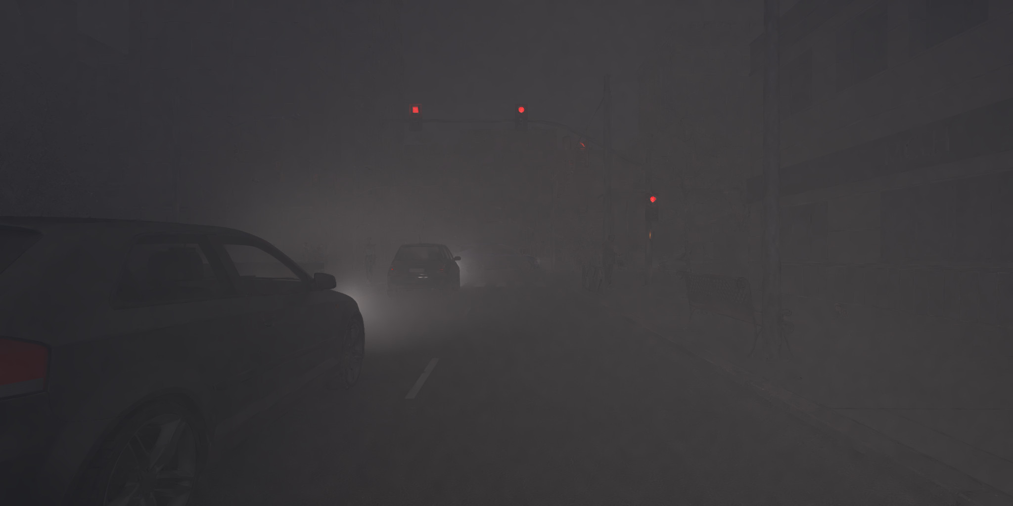
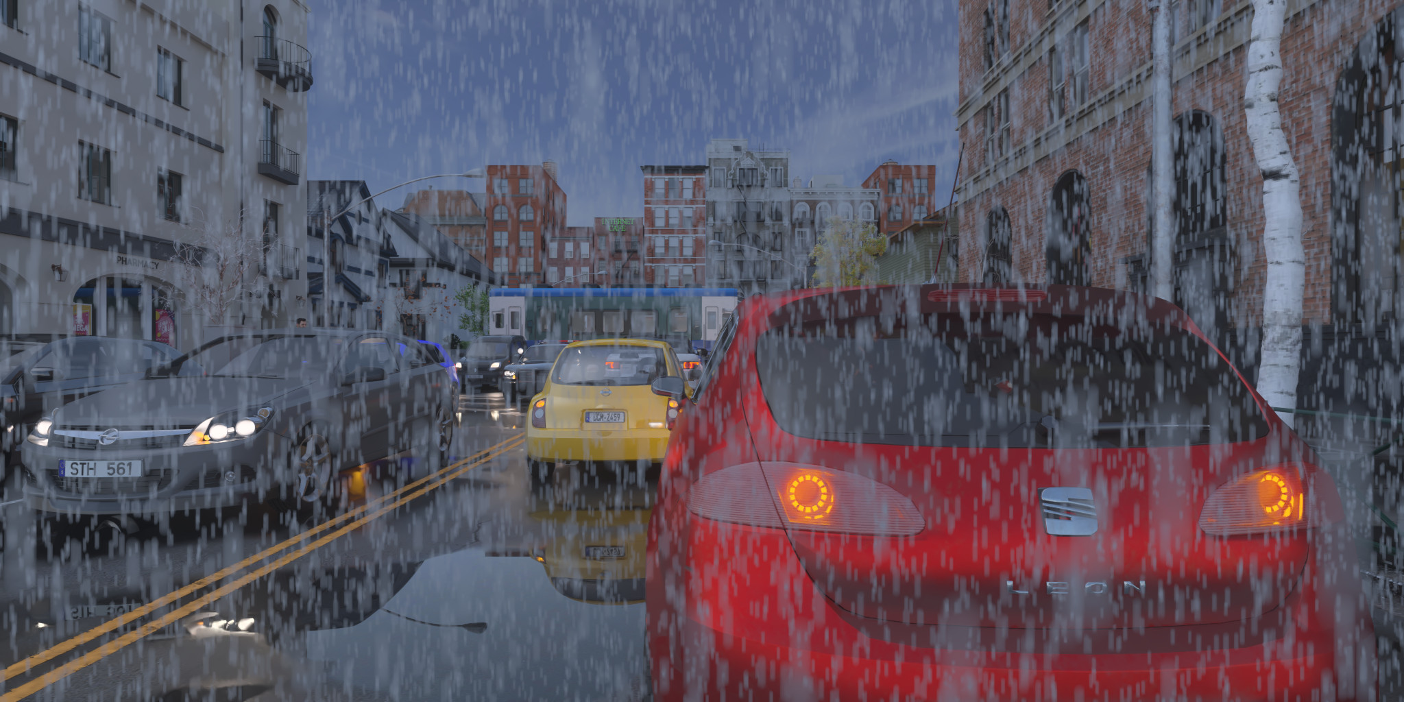
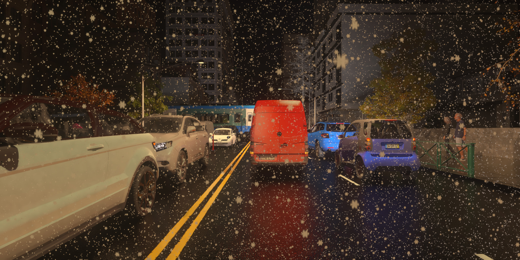
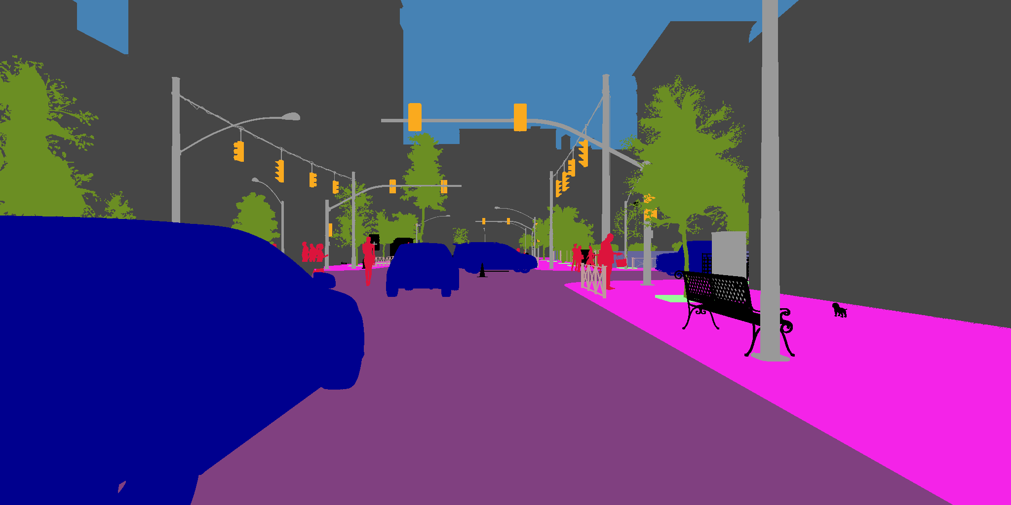
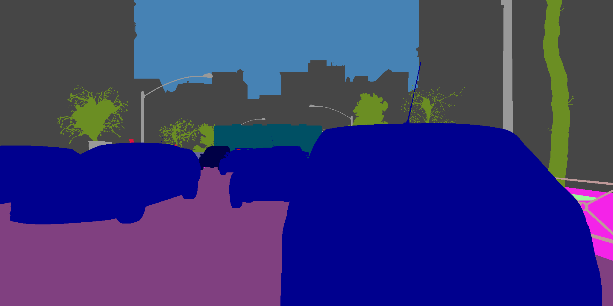
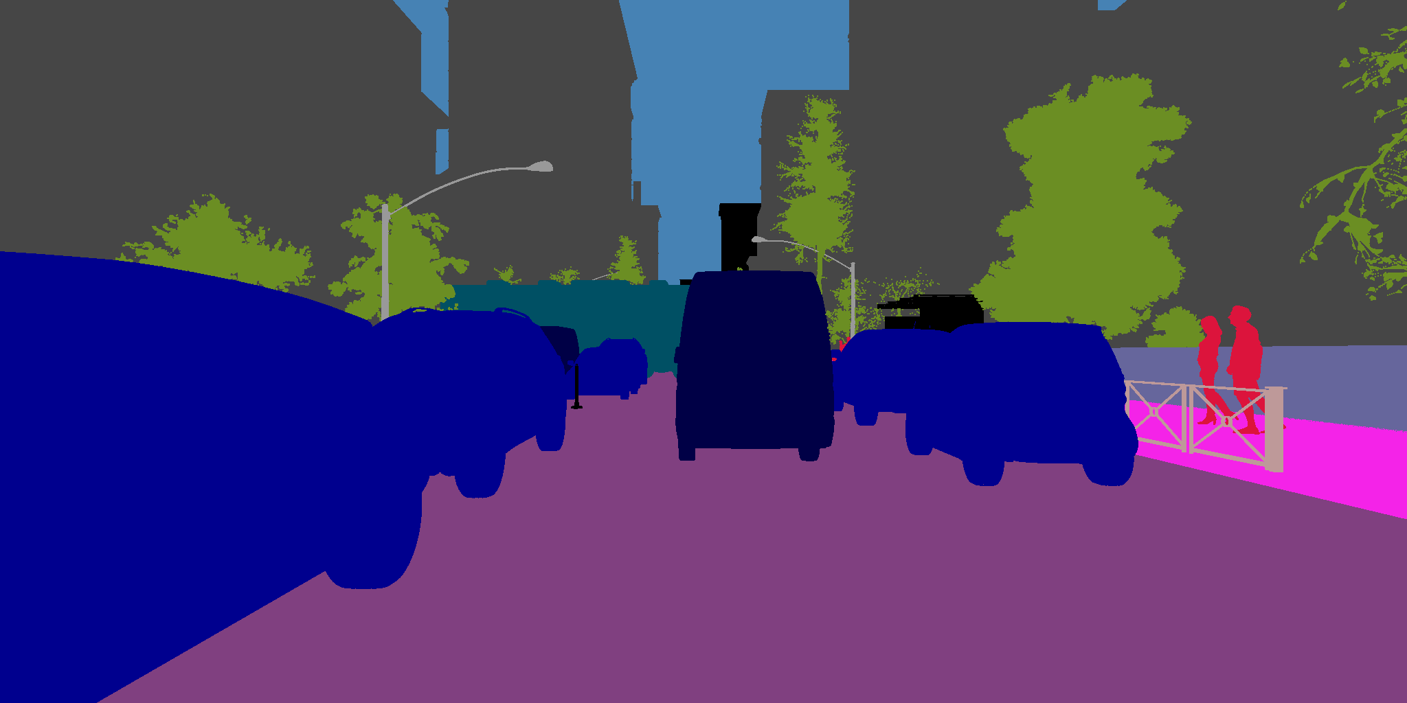
Figure 3: Illustration of semantic segmentation images of MUAD dataset. The first row is composed of the original images of the high adv. set. The second row is their corresponding ground truth.

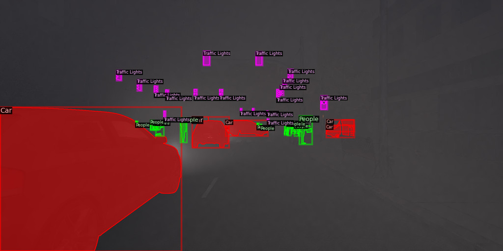
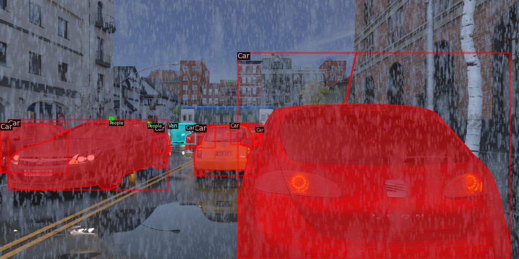
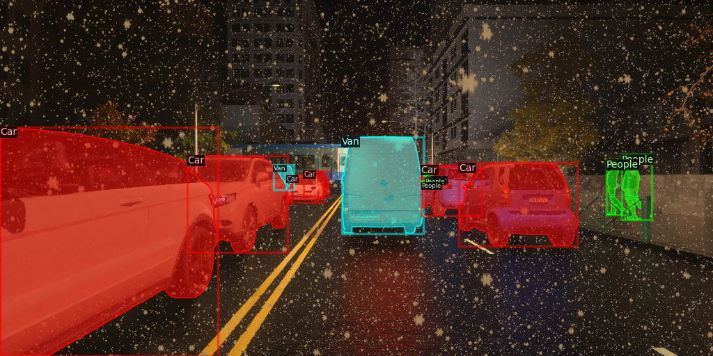
Figure 4: Illustration of instance segmentation images of MUAD dataset. The three images are selected from the high adv. set. We illustrated fog (4), rain (4), and snow (4) conditions.

Cityscapes classes	MUAD classes	nb. of images with the annotations
Road	Bots, Tram Tracks, Crosswalk, Parking Area, Garbage - Road, Road Lines, Sewer Longitudinal Crack, Transversal Crack, Road, Asphalt hole, Polished Aggregate, Vegetation - Road, Sewer - Road, Construction Concrete	9,055
Sidewalk	Lane Bike, Kerb Stone, Sidewalk, Kerb Rising Edge	8,948
Building	House, Construction Scaffold, Building, Air Conditioning, Construction Container, TV Antenna, Terrace, Water Tank, Pergola Garden, Stairs, Dog House, Sunshades, Railings, Construction Stock, Marquees, Hangar Airport	9,089
Wall	Wall	1,101
Fence	Construction Fence, Fences	8,622
Pole	Traffic Signs Poles or Structure, Traffic Lights Poles, Street lights, Lamp	8,984
Traffic light	Traffic Lights Head, Traffic Cameras, Traffic Lights Bulb (red, yellow, green)	8,222
Traffic sign	Traffic Signs	2,672
Vegetation	Vegetation	9,072
Terrain	Terrain, Tree Pit	8,377
Sky	Sky	8,591
Person	Walker, All colors of Construction Helmet, All colors of Safety Vest, Umbrella, People	8,843
Rider	Cyclist, Biker	3,470
Car	Car, Beacon Light, Van, Ego Car	9,026
Truck	Truck	5,533
Bus	Bus	0
Train	Train, Subway	2,240
Motorcycle	Motorcycle, Segway, Scooter Child	2,615
Bicycle	Bicycle, Kickbike, Tricycle	2,816
Animals	Cow, Bear, Deer, Moose	603
Objects anomalies	Food Stand, Trash Can, Garbage Bag	352
Background	Others	-

Table 2: Overview of annotated classes

3.1 MUAD statistics

Our dataset contains 3,420 images in the train set, and 492 in the validation set. The test set is composed of 6,501 images divided as follows: 551 in the normal set, 102 in the normal set no shadow, 1,668 in the OOD set, 605 in the low adv. set, 602 in the high adv. set, 1,552 in the low adv. with OOD set and 1,421 in the high adv. with OOD set. All of these sets cover day and night conditions with 2/3 of day images and 1/3 of night images. Test datasets address diverse weather conditions (rain, snow, and fog with different levels), and various OOD objects. The resolution of all images is 1024$\times$2048.

The dataset aims to provide a general and consistent coverage for a typical urban and suburban environment under different times of day and weather conditions. Ego-vehicle poses are drawn randomly within a complex environment, and in a second stage the field of view is populated stochastically with dynamic objects of interest following distributions in compliance with their expected behaviour. The pose and context changes as well as the variation of the models for the objects of interest ensure that content diversity is high, in addition to images being photorealistic. The simulator makes use of approximately 300 different person models and 150 different vehicle models, which are sampled while varying their visual characteristics.

3.2 Class labels

The class ontology of MUAD is presented in Table 2. MUAD comprises 155 different classes that we have regrouped into 21 classes. The first 19 classes are similar to the CityScapes classes [Cordts et al.(2016)Cordts, Omran, Ramos, Rehfeld, Enzweiler, Benenson, Franke, Roth, and Schiele], then we added object anomalies and animals to have more diversity in the anomalies. In addition to ensuring high content diversity, this ontology facilitates the mapping of MUAD to specific environments which require or impose a lower number of more generic classes. Consequently, trained models are easily transferable for existing datasets, and we provide the mapping towards the 21 classes widely used by the community, e.g., [Chen et al.(2017b)Chen, Chen, Chen, Tsai, Frank Wang, and Sun, Cordts et al.(2016)Cordts, Omran, Ramos, Rehfeld, Enzweiler, Benenson, Franke, Roth, and Schiele, Ros et al.(2016)Ros, Sellart, Materzynska, Vazquez, and Lopez, Richter et al.(2016)Richter, Vineet, Roth, and Koltun]. The dataset statistics for the 21 classes are presented in Figure 2. For the evaluation of OOD detection, we have excluded nine classes (train, motorcycle, bicycle, bears, cow, deers, moose, food stand, garbage bags) from the training and validation sets. These classes are present in the test set as OOD objects. DNNs that process samples belonging to one of these nine classes are expected to have a low confidence score.

3.3 Photorealistic rendering

Our physically based approach simulates the weather conditions taking into consideration the amount of ozone, the humidity, among other factors. Regarding the sky, the renderer uses a physical model of the light coming from the sky. The amount of ozone and humidity in the atmosphere changes the emissive spectral profile of the sky, impacting the color of the objects in the scene. Apart from ozone and humidity, there are other factors that the render takes into account, for instance, turbidity and scattering asymmetry. Regarding the rain and the snow, the simulation of every raindrop allows us to model physical dispersion. For improved realism we choose the falling speed and size of raindrops according to observed real rain [Muramoto et al.(1989)Muramoto, Shiina, Endoh, Konishi, Kitano, et al., baranidesign(2020)]. For snow, the same principle applies, but changing in this case the material and the dynamics. Regarding the fog, we use a full volumetric approach for the simulation where scattering effects are considered. Regarding the level of noise, to the best of our knowledge, there is no standard procedure to measure the intensity of adverse weather conditions for driving scenarios. We empirically selected the number of raindrops, snowflakes, and fog intensity from a human point or view. All the efforts mentioned above improved our dataset realism. A study [Mateos(2020)] was performed that confirmed that our render enhances the realism of MUAD compared to SYNTHIA.

4 Experiments

4.1 Semantic segmentation experiments

Methods	Architectures	normal set		low adv. without OOD set		high adv. without OOD set
		mIoU $\uparrow$	ECE $\downarrow$	mIoU $\uparrow$	ECE $\downarrow$	mIoU $\uparrow$	ECE $\downarrow$
Baseline (MCP) [Hendrycks and Gimpel(2017)]	DeepLab v3+  [Chen et al.(2018)Chen, Zhu, Papandreou, Schroff, and Adam]	68.90%	0.0138	38.77%	0.3238	22.51%	0.4567
Baseline (MCP) [Hendrycks and Gimpel(2017)]	SegFormer-B0 [Xie et al.(2021)Xie, Wang, Yu, Anandkumar, Alvarez, and Luo]	69.04%	0.0135	48.67%	0.1004	30.0%	0.2396
MC-Dropout [Gal and Ghahramani(2016)]	DeepLab v3+  [Chen et al.(2018)Chen, Zhu, Papandreou, Schroff, and Adam]	65.33%	0.0172	42.08%	0.2587	27.68%	0.3846
MC-Dropout [Gal and Ghahramani(2016)]	SegFormer-B0 [Xie et al.(2021)Xie, Wang, Yu, Anandkumar, Alvarez, and Luo]	68.55%	0.0119	45.01%	0.0758	26.59%	0.1594
Deep Ensembles  [Lakshminarayanan et al.(2017)Lakshminarayanan, Pritzel, and Blundell]	DeepLab v3+  [Chen et al.(2018)Chen, Zhu, Papandreou, Schroff, and Adam]	69.80%	0.0129	42.81%	0.2444	23.91%	0.4500
Deep Ensembles  [Lakshminarayanan et al.(2017)Lakshminarayanan, Pritzel, and Blundell]	SegFormer-B0 [Xie et al.(2021)Xie, Wang, Yu, Anandkumar, Alvarez, and Luo]	70.00%	0.0115	49.10%	0.0837	31.67%	0.3167

Methods	Architectures	OOD set					low adv. with OOD set					high adv. with OOD set
		mIoU $\uparrow$	ECE $\downarrow$	AUROC $\uparrow$	AUPR $\uparrow$	FPR $\downarrow$	mIoU $\uparrow$	ECE $\downarrow$	AUROC $\uparrow$	AUPR $\uparrow$	FPR $\downarrow$	mIoU $\uparrow$	ECE $\downarrow$	AUROC $\uparrow$	AUPR $\uparrow$	FPR $\downarrow$
Baseline (MCP) [Hendrycks and Gimpel(2017)]	DeepLab v3+  [Chen et al.(2018)Chen, Zhu, Papandreou, Schroff, and Adam]	57.32%	0.0607	0.8624	0.2604	0.3943	31.84%	0.3078	0.6349	0.1185	0.6746	18.94%	0.4356	0.6023	0.1073	0.7547
Baseline (MCP) [Hendrycks and Gimpel(2017)]	SegFormer-B0 [Xie et al.(2021)Xie, Wang, Yu, Anandkumar, Alvarez, and Luo]	58.91 %	0.06465	0.8578	0.21576	0.4106	40.22%	0.1544	0.7448	0.1361	0.5876	27.51 %	0.6564	0.6564	0.1071	0.7011
MC-Dropout [Gal and Ghahramani(2016)]	DeepLab v3+  [Chen et al.(2018)Chen, Zhu, Papandreou, Schroff, and Adam]	55.62%	0.0645	0.8439	0.2225	0.4575	33.38%	0.1329	0.7506	0.1545	0.5807	20.77%	0.3809	0.6864	0.1185	0.6751
MC-Dropout [Gal and Ghahramani(2016)]	SegFormer-B0 [Xie et al.(2021)Xie, Wang, Yu, Anandkumar, Alvarez, and Luo]	58.81%	0.0574	0.8811	0.2535	0.3435	39.64%	0.1172	0.7698	0.1557	0.5498	26.52%	0.1771	0.6965	0.1237	0.6633
Deep Ensembles  [Lakshminarayanan et al.(2017)Lakshminarayanan, Pritzel, and Blundell]	DeepLab v3+  [Chen et al.(2018)Chen, Zhu, Papandreou, Schroff, and Adam]	58.29%	0.0588	0.871	0.2802	0.3760	34.91%	0.2447	0.6543	0.1212	0.6425	20.19%	0.4227	0.6101	0.1162	0.7212
Deep Ensembles  [Lakshminarayanan et al.(2017)Lakshminarayanan, Pritzel, and Blundell]	SegFormer-B0 [Xie et al.(2021)Xie, Wang, Yu, Anandkumar, Alvarez, and Luo]	59.50%	0.05928	0.8843	0.2611	0.3342	40.00 %	0.1400	0.6933	0.1198	0.6290	25.89 %	0.3305	0.5939	0.0959	0.7287

Table 3: Comparative results for semantic segmentation on MUAD. The mIoU is related to the main task performance, while the rest of the metrics evaluate the uncertainty quality when the model is confronted with different types of perturbations.

Our semantic segmentation study consists of two experiments. Firstly, we evaluate on MUAD the uncertainty quantification of three benchmarks (MCP [Hendrycks and Gimpel(2017)], Deep Ensembles  [Lakshminarayanan et al.(2017)Lakshminarayanan, Pritzel, and Blundell], MC Dropout [Gal and Ghahramani(2016)]), by taking advantage of the OOD/adverse weather splits. The second experiment evaluates the quality of transfer learning from MUAD to Cityscapes [Cordts et al.(2016)Cordts, Omran, Ramos, Rehfeld, Enzweiler, Benenson, Franke, Roth, and Schiele] and the quality of the uncertainty quantification on Cityscapes. We aim here to verify whether MUAD can be used for unsupervised domain adaptation.

For the first experiment, we train a DeepLabV3+ [Chen et al.(2018)Chen, Zhu, Papandreou, Schroff, and Adam] network with ResNet50 encoder [He et al.(2016)He, Zhang, Ren, and Sun] and a SegFormer-B0 [Xie et al.(2021)Xie, Wang, Yu, Anandkumar, Alvarez, and Luo] on MUAD. Table 3 shows the results of our three baselines. The first criterion we use is the mIoU [Jaccard(1912)], and the second criterion is the expected calibration error (ECE) [Guo et al.(2017)Guo, Pleiss, Sun, and Weinberger] that measures how the confidence score predicted by a DNN is related to its accuracy. Finally, we use the AUPR, AUROC, and the FPR-95-TPR defined in [Hendrycks and Gimpel(2017)] that evaluate the quality of a DNN to detect OOD data. We can see that Deep Ensembles outperform other strategies, especially when mixed with Transformers. Yet, MC Dropout seems to have better performance on more complicated sets. Hence MUAD is well suited for quantifying the uncertainty evaluation of different DNNs.

Training set	mIoU $\uparrow$
Baseline trained on Cityscapes	76.84%
Baseline trained on MUAD	16.71%
Baseline trained on MUAD with histogram eq.	32.12%
Baseline trained on GTA [Richter et al.(2016)Richter, Vineet, Roth, and Koltun]	32.85%
Baseline trained on SYNTHIA [Ros et al.(2016)Ros, Sellart, Materzynska, Vazquez, and Lopez]	29.45%

Table 4: Comparative results for semantic segmentation simple domain adaptation from MUAD to Cityscapes. First row is the original baseline, the second row is the performance of the model trained directly on MUAD and the third row is the performance of the model trained on MUAD with histogram matching technique.

For the second experiment, we train a DeepLabV3+ [Chen et al.(2018)Chen, Zhu, Papandreou, Schroff, and Adam] segmentation network on MUAD and evaluate it on Cityscapes. Results reported in Table 4 show that models trained on MUAD images modified with simple histogram matching [Trahanias and Venetsanopoulos(1992)] with Cityscapes images achieve the same performance as models trained on the much larger GTA dataset [Richter et al.(2016)Richter, Vineet, Roth, and Koltun].

4.2 Monocular depth experiments

We provide results for monocular depth using NeWCRFs [Yuan et al.(2022)Yuan, Gu, Dai, Zhu, and Tan], which is one of the SOTA on KITTI dataset [Geiger et al.(2012)Geiger, Lenz, and Urtasun]. NeWCRFs does not output uncertainty by default. Similarly to [Nix and Weigend(1994), Kendall and Gal(2017), Ilg et al.(2018)Ilg, Cicek, Galesso, Klein, Makansi, Hutter, and Brox], we modify the DNN to output the parameters of a Gaussian distribution (i.e., the mean and variance). We denote the result as single predictive uncertainty (Single-PU). Based on this modification we train a Deep Ensembles [Lakshminarayanan et al.(2017)Lakshminarayanan, Pritzel, and Blundell] with 3 DNNs. We also provide the results from SLURP [Yu et al.(2021)Yu, Franchi, and Aldea], which needs 2 DNNs to predict the depth and the uncertainty respectively, and MC-Dropout [Gal and Ghahramani(2016)]. For depth evaluation, we use the same metrics as Eigen et al. [Eigen et al.(2014)Eigen, Puhrsch, and Fergus] which are used in many following works [Lee et al.(2019)Lee, Han, Ko, and Suh, Yuan et al.(2022)Yuan, Gu, Dai, Zhu, and Tan]. For uncertainty quality evaluation, we follow the implementation of Poggi et al. [Poggi et al.(2020)Poggi, Aleotti, Tosi, and Mattoccia]. More details on implementation and evaluation criteria are provided in the Supplementary Material.

Table 5 lists some of the depth and uncertainty results of the above techniques on our dataset due to the space limit. We observe that in the presence of OOD, the uncertainty results of Deep Ensembles are comparatively better, while MC-Dropout provides more robust depth estimations under different perturbation. Additionally, we provide self-supervised monocular depth results using left-right image consistency [Godard et al.(2017)Godard, Mac Aodha, and Brostow], along with the full supervised results in Supplementary Material. We also propose a baseline method for depth domain adaptation from MUAD to KITTI and report its performance in Table 6. Compared to the direct adaptation from Virtual KITTI 2 [Gaidon et al.(2016)Gaidon, Wang, Cabon, and Vig], which is specifically designed based on the target dataset KITTI [Geiger et al.(2012)Geiger, Lenz, and Urtasun], the model trained on MUAD can achieve competitive performance.

Methods	normal set					low adv. without OOD set					high adv. without OOD set					normal set overhead sun
	Depth results			Uncertainty results		Depth results			Uncertainty results		Depth results			Uncertainty results		Depth results			Uncertainty results
	d1 $\uparrow$	AbsRel $\downarrow$	RMSE $\downarrow$	AUSE RMSE $\downarrow$	AUSE Absrel $\downarrow$	d1 $\uparrow$	AbsRel $\downarrow$	RMSE $\downarrow$	AUSE RMSE $\downarrow$	AUSE Absrel $\downarrow$	d1 $\uparrow$	AbsRel $\downarrow$	RMSE $\downarrow$	AUSE RMSE $\downarrow$	AUSE Absrel $\downarrow$	d1 $\uparrow$	AbsRel $\downarrow$	RMSE $\downarrow$	AUSE RMSE $\downarrow$	AUSE Absrel $\downarrow$
Baseline	0.922	0.114	3.357	-	-	0.786	0.147	5.005	-	-	0.632	0.207	6.989	-	-	0.951	0.090	3.646	-	-
Deep Ensembles [Lakshminarayanan et al.(2017)Lakshminarayanan, Pritzel, and Blundell]	0.929	0.111	3.199	0.291	0.060	0.767	0.156	4.892	0.740	0.105	0.566	0.243	7.498	1.182	0.153	0.955	0.083	3.479	0.336	0.055
MC Dropout [Gal and Ghahramani(2016)]	0.919	0.119	3.209	0.634	0.061	0.798	0.151	4.580	1.063	0.098	0.657	0.207	6.278	1.382	0.128	0.948	0.092	3.407	0.786	0.058
Single-PU [Kendall and Gal(2017)]	0.905	0.132	3.230	0.313	0.081	0.773	0.159	4.865	0.789	0.112	0.571	0.248	7.680	1.740	0.171	0.946	0.105	3.546	0.358	0.079
SLURP [Yu et al.(2021)Yu, Franchi, and Aldea]	0.922	0.114	3.357	0.467	0.048	0.786	0.147	5.005	1.167	0.090	0.632	0.207	6.989	1.707	0.128	0.951	0.090	3.646	0.525	0.033

Methods	OOD set					low adv. with OOD set					high adv. with OOD set
	Depth results			Uncertainty results		Depth results			Uncertainty results		Depth results			Uncertainty results
	d1 $\uparrow$	AbsRel $\downarrow$	RMSE $\downarrow$	AUSE RMSE $\downarrow$	AUSE Absrel $\downarrow$	d1 $\uparrow$	AbsRel $\downarrow$	RMSE $\downarrow$	AUSE RMSE $\downarrow$	AUSE Absrel $\downarrow$	d1 $\uparrow$	AbsRel $\downarrow$	RMSE $\downarrow$	AUSE RMSE $\downarrow$	AUSE Absrel $\downarrow$
Baseline	0.896	0.125	3.616	-	-	0.713	2.637	4.764	-	-	0.555	0.459	6.916	-	-
Deep Ensembles [Lakshminarayanan et al.(2017)Lakshminarayanan, Pritzel, and Blundell]	0.903	0.114	3.447	0.427	0.074	0.709	1.810	4.707	0.692	0.129	0.521	0.331	7.411	1.072	0.151
MC Dropout [Gal and Ghahramani(2016)]	0.893	0.145	3.432	0.724	0.080	0.744	3.925	4.364	0.927	0.206	0.610	0.545	6.176	1.245	0.314
Single-PU [Kendall and Gal(2017)]	0.888	0.132	3.463	0.447	0.095	0.714	4.349	4.716	0.744	0.482	0.529	0.351	7.627	1.347	0.156
SLURP [Yu et al.(2021)Yu, Franchi, and Aldea]	0.896	0.125	3.616	0.721	0.068	0.713	2.637	4.764	1.072	0.212	0.555	0.459	6.916	1.564	0.151

Table 5: Comparative results for monocular depth on MUAD. We use NeWCRFs [Yuan et al.(2022)Yuan, Gu, Dai, Zhu, and Tan] as the based DNN for monocular depth task.

	KITTI
Training set	d1$\uparrow$	d2$\uparrow$	d3$\uparrow$	Abs Rel$\downarrow$	Sq Rel$\downarrow$	RMSE$\downarrow$	RMSE log$\downarrow$	SILog$\downarrow$
KITTI [Geiger et al.(2012)Geiger, Lenz, and Urtasun]	0.975	0.997	0.999	0.052	0.148	2.072	0.078	6.9859
Virtual KITTI 2 [Cabon et al.(2020)Cabon, Murray, and Humenberger]	0.835	0.957	0.989	0.129	0.706	4.039	0.177	15.534
MUAD	0.731	0.927	0.983	0.187	1.059	4.754	0.227	18.581

Table 6: Comparative results for monocular depth estimation simple domain adaptation from MUAD to KITTI eigen-split [Eigen et al.(2014)Eigen, Puhrsch, and Fergus]. First row is the original baseline, the second and the third rows are the performance of the model trained directly on Virtual KITTI 2 [Gaidon et al.(2016)Gaidon, Wang, Cabon, and Vig] and MUAD respectively.

4.3 Object detection experiments

Evaluation data	normal set			low adv. without OOD set			high adv. without OOD set			OOD set			low adv. with OOD set			high adv. with OOD set
	mAP $\uparrow$	AP50 $\uparrow$	PDQ $\uparrow$	mAP $\uparrow$	AP50 $\uparrow$	PDQ $\uparrow$	mAP $\uparrow$	AP50 $\uparrow$	PDQ $\uparrow$	mAP $\uparrow$	AP50 $\uparrow$	PDQ $\uparrow$	mAP $\uparrow$	AP50 $\uparrow$	PDQ $\uparrow$	mAP $\uparrow$	AP50 $\uparrow$	PDQ $\uparrow$
Faster R-CNN (ResNet101)	39.91%	54.91%	16.88%	25.00%	36.89%	8.61	13.97%	22.01%	0.041	35.85%	48.9%	14.33%	24.73%	35.70%	8.49%	12.41%	19.66%	3.86%
Faster R-CNN (ResNet50)	38.43%	53.13%	15.02%	25.19%	37.38%	8.18%	13.29%	21.53%	0.0389%	34.52%	47.63%	12.96%	23.93%	34.51%	7.95%	12.11%	19.46%	3.64%
Gaussian YOLOV3  [Choi et al.(2019)Choi, Chun, Kim, and Lee]	20.81%	32.84%	2.22%	8.79%	16.40%	0.57%	3.28%	6.30%	0.22%	17.44%	28.16%	1.52%	10.80%	18.71%	0.64%	3.21%	6.15%	0.26%

Table 7: Comparative results for object detection on MUAD. The first criteria are the mAP AP50 [Lin et al.(2014)Lin, Maire, Belongie, Hays, Perona, Ramanan, Dollár, and Zitnick] related to the accuracy, and the second criterion is the PDQ [Hall et al.(2020)Hall, Dayoub, Skinner, Zhang, Miller, Corke, Carneiro, Angelova, and Sünderhauf] that measures how well detectors probabilistically localise objects in an image.

For the object detection task, we trained a Gaussian YOLOV3 [Choi et al.(2019)Choi, Chun, Kim, and Lee] and a Faster-RCNN [Ren et al.(2015a)Ren, He, Girshick, and Sun] on the training data. The Faster R-CNN are trained with ResNet101 and ResNet50 backbones with FPN [Lin et al.(2017)Lin, Dollár, Girshick, He, Hariharan, and Belongie]. All the results are presented on Table 7. We can see that Faster R-CNN’s performance drops with the adversarial conditions, which confirms that considering the adversarial behavior is important when designing algorithms.

4.4 Discussion

The experiments show that the best main task contender might not always be the most suited against different sources of uncertainty, thus it is important to test thoroughly and adapt the processing pipeline to the expected type of perturbations. The similar ranking of methods on our synthetic dataset and on real data (see [Hendrycks et al.(2019)Hendrycks, Basart, Mazeika, Mostajabi, Steinhardt, and Song, Franchi et al.(2021)Franchi, Belkhir, Ha, Hu, Bursuc, Blanz, and Yao]) is encouraging as it allows us to generalize the analysis performed on MUAD to actual scenarios. An additional benefit of synthetic datasets is related to the reduced data privacy concerns and regulations that typically affect real world datasets, in particular in urban settings that include pedestrians. All these traits allow for faster validation of new algorithms before their deployment in in real-world settings. Finally, a potential different usage of MUAD concerns unsupervised domain adaptation from synthetic to real domains. Our preliminary results are encouraging.

5 Conclusion

Previous research in deep learning and autonomous cars has established that it is essential to robustify DNNs. In this paper, we present MUAD, a synthetic but highly realistic dataset incorporating multiples sources of uncertainties for autonomous driving, that provides insight into the robustness of DNNs for various applications. Based on MUAD, we provide a set of baselines for three fundamental computer vision tasks. Uncertainty is related to events that occur rarely; synthetic data is very valuable for dealing with infrequent events. We hope that our dataset can improve the reliability of DNNs, especially in autonomous driving scenarios. We are the first, to our knowledge, to provide a dataset with such noise dichotomies present in automotive applications. Our extensive benchmarks show the greater than ever importance of considering uncertainty quantification in addition to accuracy, for decision making systems in sensitive applications.

MUAD: Multiple Uncertainties for Autonomous Driving, a benchmark for multiple uncertainty types and tasks (Supplementary Material)

Gianni Franchigianni.franchi@ensta-paris.fr1$\dagger$ Xuanlong Yuxuanlong.yu@universite-paris-saclay.fr1,2$\dagger$ Andrei Bursucandrei.bursuc@valeo.com3 Angel Tenaangel.tena@anyverse.ai4 Rémi Kazmierczakremi.kazmierczak@ensta-paris.fr1 Séverine Dubuissonseverine.dubuisson@lis-lab.fr5 Emanuel Aldeaemanuel.aldea@universite-paris-saclay.fr2 David Filliatdavid.filliat@ensta-paris.fr1 U2IS, ENSTA Paris, IP Paris SATIE, Paris-Saclay University valeo.ai Anyverse Aix Marseille University

Dataset with Multiple Uncertainties for Autonomous Driving

MUAD: Multiple Uncertainties for Autonomous Driving, a benchmark for multiple uncertainty types and tasks
— Supplementary Material —

Appendix A Multiple Uncertainties for Autonomous Driving benchmark (MUAD)

A.1 Uncertainty and Deep Learning

A DNN is a function $f_{\theta}$ parameterized by a set of parameters $\theta$ that takes input data $x$ and outputs a prediction $y$. The DNN is trained on a training dataset composed of a set $\mathcal{D}=\{x_{i},y_{i}\}_{i=1}^{N}$, with $N$ being the number of data to optimize the parameters $\theta$ for a task. Once the DNN is trained, meaning that the optimization of $\theta$ on $\mathcal{D}$ is completed, $f_{\theta}$ may be used for inference on new data $x^{*}$.

Uncertainty on deep learning may arise mainly from three factors [Gawlikowski et al.(2021)Gawlikowski, Tassi, Ali, Lee, Humt, Feng, Kruspe, Triebel, Jung, Roscher, et al.]. Firstly it can result from the data acquisition process which introduces some noise. This might be due to the variability in real-world situations. For example, one records training data in certain weather conditions, which subsequently change during inferences. The measurement systems might also introduce errors such as sensor noise. Secondly, uncertainty may result from the DNN building and training process. DNNs are random functions whose parameters $\theta$ are initialized randomly and whose training procedure relies on stochastic optimization. Therefore, the resulting neural network is a random function that is most of the time related to a local minimum of the expected loss function (which we denote as the risk). Hence this source of randomness might cause errors in the training procedure of the DNN. Thirdly, the last uncertainty factor is related to the DNN’s prediction’s uncertainty. Uncertainty could come from the lack of knowledge of the DNN and might be caused by unknown test data.

Based on these factors, we can divide the uncertainty into two kinds: the aleatoric uncertainty and the epistemic uncertainty. The aleatoric uncertainty can be subdivided into two kinds: In-domain uncertainty [Ashukha et al.(2020)Ashukha, Lyzhov, Molchanov, and Vetrov] and Domain-shift uncertainty [Ovadia et al.(2019)Ovadia, Fertig, Ren, Nado, Sculley, Nowozin, Dillon, Lakshminarayanan, and Snoek]. In-domain uncertainty occurs when the test data is sampled from the training distribution and is related to the inability of the deep neural network to predict a proper confidence score about the quality of its predictions due to a lack of in-domain knowledge. Domain-shift uncertainty denotes the uncertainty related to an input drawn from a shifted version of the training distribution. Hence, it is caused by the fact the distribution of the training dataset might not encompass enough variability. These two kinds of uncertainty can be reduced by increasing the number of the training dataset. Epistemic uncertainty denotes the uncertainty when the test data is sampled from a distribution that is different and far from the training distribution. Epistemic uncertainty can be categorized into two kinds namely [Tuna et al.(2021)Tuna, Catak, and Eskil] : approximation uncertainty and model uncertainty. The approximation uncertainty is linked to the fact that we optimize the empirical risk instead of the risk. Hence, the optimal DNN’s parameters approximate the optimal DNN’s parameters of the true risk function. The model uncertainty is linked to the fact that our loss function provides us with a space of solutions that might not include the perfect predictor. For example, the DNN might have different classes between the training and testing set. In this context ’Out of Distribution’ samples refers to anomalies in the test set that are data from classes not present in the training set.

Appendix B Extra Monocular depth experiments

B.1 Implementation and criterion

Implementation.   We train the NeWCRFs [Yuan et al.(2022)Yuan, Gu, Dai, Zhu, and Tan] model using the same hyperparameters and image augmentation parameters used in the official paper for training on KITTI [Geiger et al.(2012)Geiger, Lenz, and Urtasun], except that we change the batch size to 4 and randomly crop the input image to 512*1024. For the Single-PU [Kendall and Gal(2017)] models, we perform a multi task training where we train to predict the depth map with the silog loss function provided in the NeWCRFs [Yuan et al.(2022)Yuan, Gu, Dai, Zhu, and Tan] paper, and we minimize the negative Gaussian log-likelihood loss in order to train to predict the variance. To train the DNN that will predict the variance, we do not optimize the layers that are used to predict the depth map, as explained in [Asai et al.(2019)Asai, Ikami, and Aizawa], as this stabilizes the training. Regarding MC-Dropout [Gal and Ghahramani(2016)], we let the dropout layers activated during the inference and perform eight forward passes for each input data during inference and average the predictions. We want to point out that we did not add any additional dropout layers to the model to keep the paper’s performance. For the SLURP [Yu et al.(2021)Yu, Franchi, and Aldea] models, we use the base model as the main task model and train an auxiliary uncertainty estimator. We use the Swin Transformer [Liu et al.(2021)Liu, Lin, Cao, Hu, Wei, Zhang, Lin, and Guo] as used in the base model as an encoder for the auxiliary model and train the auxiliary model for 20 epochs.
Evaluation metrics.   To evaluate depth estimations, we use the same metrics as Eigen et al [Eigen et al.(2014)Eigen, Puhrsch, and Fergus] which are standard criteria [Lee et al.(2019)Lee, Han, Ko, and Suh, Zhou et al.(2021)Zhou, Greenwood, and Taylor, Yuan et al.(2022)Yuan, Gu, Dai, Zhu, and Tan]. For uncertainty quantification evaluation metrics, we use the criteria implementation of Poggi et al [Poggi et al.(2020)Poggi, Aleotti, Tosi, and Mattoccia]: Area Under the Sparsification Error (AUSE) and Area Under the Random Gain (AURG). The Area Under the Sparsification Error is obtained by calculating the difference between the sparsification curve and the oracle sparsification curve. The sparsification curve is obtained by continuously erasing 1% pixels according to the predicted uncertainty and calculating the prediction error for the rest pixels. We can also have an oracle sparsification curve by continuously erasing pixels according to their prediction error. The total difference between the two curves is AUSE. We can evaluate the AUSE for different error metrics such as RMSE, Absrel, and d1, which provide us AUSE-RMSE, AUSE-Absrel, and AUSE-d1. AURG is achieved by calculating the area between the Sparsification curve and a random curve to measure how good the uncertainty estimator is compared to no modeling cases. Similarly, we can achieve AURG-RMSE, AURG-Absrel, and AURG-d1 using different error metrics.

B.2 Full results on supervised monocular depth estimation

In the main paper, due to the space constrain, we can only provide partial results for depth and uncertainty metrics, we here provide full results from Table 5 to Table 11 for different uncertainty quantification solutions introduced in the main paper applied on supervised monocular depth estimation task. Overall, the Deep Ensembles [Lakshminarayanan et al.(2017)Lakshminarayanan, Pritzel, and Blundell] and SLURP [Yu et al.(2021)Yu, Franchi, and Aldea] can provide better uncertainty estimations on the test sets without perturbations. When weather perturbations exist, MC-Dropout [Gal and Ghahramani(2016)] and Deep Ensembles [Lakshminarayanan et al.(2017)Lakshminarayanan, Pritzel, and Blundell] perform better on uncertainty quantification. MC-Dropout can also provide better depth estimations than the other solutions under weather perturbations.

Methods	silog$\downarrow$	AbsRel$\downarrow$	log10$\downarrow$	RMSE$\downarrow$	SqRel$\downarrow$	log_RMSE	d1$\uparrow$	d2$\uparrow$	d3$\uparrow$	AUSE$\downarrow$			AURG$\uparrow$
										AbsRel	RMSE	d1	AbsRel	RMSE	d1
Baseline	13.9767	0.1143	0.0444	3.3575	0.5571	0.1443	0.9219	0.9833	0.9933	-	-	-	-	-	-
Deep Ensembles [Lakshminarayanan et al.(2017)Lakshminarayanan, Pritzel, and Blundell]	13.6691	0.1110	0.0419	3.1994	0.6076	0.1400	0.9289	0.9843	0.9945	0.0604	0.2906	0.0431	0.0117	2.4618	0.0215
MC Dropout [Gal and Ghahramani(2016)]	13.5602	0.1194	0.0447	3.2090	0.6897	0.1453	0.9193	0.9847	0.9941	0.0610	0.6339	0.0542	0.0161	2.0846	0.0193
Single-PU [Kendall and Gal(2017)]	14.5896	0.1324	0.0484	3.2298	0.7738	0.1547	0.9054	0.9803	0.9933	0.0807	0.3131	0.0837	0.0042	2.4194	-0.0005
SLURP [Yu et al.(2021)Yu, Franchi, and Aldea]	13.9767	0.1143	0.0444	3.3575	0.5571	0.1443	0.9219	0.9833	0.9933	0.0477	0.4672	0.0459	0.0252	2.3870	0.0237

Table 5: Supervised monocular depth results on normal set.

Methods	silog$\downarrow$	AbsRel$\downarrow$	log10$\downarrow$	RMSE$\downarrow$	SqRel$\downarrow$	log_RMSE	d1$\uparrow$	d2$\uparrow$	d3$\uparrow$	AUSE$\downarrow$			AURG$\uparrow$
										AbsRel	RMSE	d1	AbsRel	RMSE	d1
Baseline	19.8427	0.1474	0.0757	5.0053	0.8301	0.2397	0.7861	0.9244	0.9613	-	-	-	-	-	-
Deep Ensembles [Lakshminarayanan et al.(2017)Lakshminarayanan, Pritzel, and Blundell]	22.7950	0.1564	0.0850	4.8919	0.8508	0.2759	0.7673	0.9010	0.9419	0.1047	0.7401	0.1823	-0.0103	3.1624	0.0023
MC Dropout [Gal and Ghahramani(2016)]	21.6959	0.1505	0.0765	4.5799	0.7648	0.2459	0.7980	0.9199	0.9543	0.0980	1.0627	0.1473	-0.0074	2.5851	0.0182
Single-PU [Kendall and Gal(2017)]	24.2069	0.1588	0.0849	4.8648	0.8522	0.2800	0.7727	0.8997	0.9417	0.1115	0.7892	0.1863	-0.0145	3.1099	-0.0025
SLURP [Yu et al.(2021)Yu, Franchi, and Aldea]	19.8429	0.1474	0.0757	5.0053	0.8301	0.2397	0.7861	0.9244	0.9613	0.0898	1.1665	0.1789	-0.0040	2.8036	-0.0037

Table 6: Supervised monocular depth results on low adv. without OOD set.

Methods	silog$\downarrow$	AbsRel$\downarrow$	log10$\downarrow$	RMSE$\downarrow$	SqRel$\downarrow$	log_RMSE	d1$\uparrow$	d2$\uparrow$	d3$\uparrow$	AUSE$\downarrow$			AURG$\uparrow$
										AbsRel	RMSE	d1	AbsRel	RMSE	d1
Baseline	27.2917	0.2072	0.1148	6.9890	1.5990	0.3603	0.6316	0.8275	0.9028	-	-	-	-	-	-
Deep Ensembles [Lakshminarayanan et al.(2017)Lakshminarayanan, Pritzel, and Blundell]	34.7624	0.2429	0.1478	7.4977	1.9794	0.4674	0.5657	0.7643	0.8507	0.1529	1.1824	0.3031	-0.0117	4.6140	-0.0044
MC Dropout [Gal and Ghahramani(2016)]	30.5442	0.2073	0.1142	6.2782	1.3762	0.3652	0.6567	0.8292	0.8992	0.1277	1.3819	0.2169	-0.0055	3.5187	0.0393
Single-PU [Kendall and Gal(2017)]	41.9847	0.2480	0.1588	7.6797	2.1362	0.5295	0.5708	0.7586	0.8435	0.1706	1.7402	0.3318	-0.0220	4.2634	-0.0322
SLURP [Yu et al.(2021)Yu, Franchi, and Aldea]	27.2917	0.2072	0.1148	6.9890	1.5990	0.3603	0.6316	0.8275	0.9028	0.1281	1.7066	0.2740	-0.0100	3.7188	-0.0024

Table 7: Supervised monocular depth results on high adv. without OOD set.

Methods	silog$\downarrow$	AbsRel$\downarrow$	log10$\downarrow$	RMSE$\downarrow$	SqRel$\downarrow$	log_RMSE	d1$\uparrow$	d2$\uparrow$	d3$\uparrow$	AUSE$\downarrow$			AURG$\uparrow$
										AbsRel	RMSE	d1	AbsRel	RMSE	d1
Baseline	12.4227	0.0895	0.0387	3.6461	0.4083	0.1257	0.9513	0.9909	0.9969	-	-	-	-	-	-
Deep Ensembles [Lakshminarayanan et al.(2017)Lakshminarayanan, Pritzel, and Blundell]	11.7212	0.0829	0.0351	3.4788	0.3867	0.1188	0.9553	0.9903	0.9967	0.0553	0.3363	0.0098	-0.0041	2.6248	0.0336
MC Dropout [Gal and Ghahramani(2016)]	12.0129	0.0915	0.0389	3.4074	0.3888	0.1263	0.9475	0.9902	0.9969	0.0576	0.7856	0.0308	-0.0019	2.0452	0.0199
Single-PU [Kendall and Gal(2017)]	12.4754	0.1052	0.0437	3.5463	0.4210	0.1344	0.9461	0.9895	0.9966	0.0788	0.3576	0.0308	-0.0189	2.5430	0.0212
SLURP [Yu et al.(2021)Yu, Franchi, and Aldea]	12.4227	0.0895	0.0387	3.6461	0.4083	0.1257	0.9513	0.9909	0.9969	0.0328	0.5248	0.0100	0.0222	2.5207	0.0373

Table 8: Supervised monocular depth results on normal test set with Overhead Sun.

Methods	silog$\downarrow$	AbsRel$\downarrow$	log10$\downarrow$	RMSE$\downarrow$	SqRel$\downarrow$	log_RMSE	d1$\uparrow$	d2$\uparrow$	d3$\uparrow$	AUSE$\downarrow$			AURG$\uparrow$
										AbsRel	RMSE	d1	AbsRel	RMSE	d1
Baseline	16.4332	0.1250	0.0525	3.6157	0.5875	0.1747	0.8956	0.9602	0.9783	-	-	-	-	-	-
Deep Ensembles [Lakshminarayanan et al.(2017)Lakshminarayanan, Pritzel, and Blundell]	16.3795	0.1142	0.0503	3.4465	0.4812	0.1724	0.9027	0.9600	0.9777	0.0739	0.4268	0.0563	-0.0016	2.4750	0.0296
MC Dropout [Gal and Ghahramani(2016)]	16.1976	0.1277	0.0525	3.4437	0.5923	0.1744	0.8934	0.9620	0.9799	0.0720	0.7253	0.0649	0.0104	2.1331	0.0292
Single-PU [Kendall and Gal(2017)]	17.1019	0.1319	0.0561	3.4628	0.5126	0.1833	0.8884	0.9580	0.9777	0.0948	0.4474	0.0872	-0.0135	2.4091	0.0103
SLURP [Yu et al.(2021)Yu, Franchi, and Aldea]	16.4332	0.1250	0.0525	3.6157	0.5875	0.1747	0.8956	0.9602	0.9783	0.0681	0.7208	0.0852	0.0121	2.2899	0.0054

Table 9: Supervised monocular depth results on OOD set.

Methods	silog$\downarrow$	AbsRel$\downarrow$	log10$\downarrow$	RMSE$\downarrow$	SqRel$\downarrow$	log_RMSE	d1$\uparrow$	d2$\uparrow$	d3$\uparrow$	AUSE$\downarrow$			AURG$\uparrow$
										AbsRel	RMSE	d1	AbsRel	RMSE	d1
Baseline	24.2098	2.6367	0.0980	4.7962	10.3942	0.3066	0.7134	0.8775	0.9280	-	-	-	-	-	-
Deep Ensembles [Lakshminarayanan et al.(2017)Lakshminarayanan, Pritzel, and Blundell]	25.9658	1.8097	0.1009	4.7072	5.1183	0.3237	0.7091	0.8652	0.9174	0.1292	0.6917	0.2091	0.1164	3.1474	0.0067
MC Dropout [Gal and Ghahramani(2016)]	25.3372	3.9252	0.0924	4.3635	22.9193	0.2971	0.7437	0.8829	0.9287	0.2062	0.9267	0.1843	0.0598	2.6365	0.0125
Single-PU [Kendall and Gal(2017)]	27.3008	4.3492	0.1009	4.7161	28.5999	0.3284	0.7140	0.8638	0.9174	0.4815	0.7444	0.2104	-0.0210	3.1238	0.0039
SLURP [Yu et al.(2021)Yu, Franchi, and Aldea]	24.2098	2.6366	0.0980	4.7962	10.3930	0.3066	0.7134	0.8775	0.9280	0.2116	1.0715	0.2229	0.0682	2.8043	-0.0116

Table 10: Supervised monocular depth results on low adv. with OOD set.

Methods	silog$\downarrow$	AbsRel$\downarrow$	log10$\downarrow$	RMSE$\downarrow$	SqRel$\downarrow$	log_RMSE	d1$\uparrow$	d2$\uparrow$	d3$\uparrow$	AUSE$\downarrow$			AURG$\uparrow$
										AbsRel	RMSE	d1	AbsRel	RMSE	d1
Baseline	32.1516	0.4588	0.1448	6.9160	10.0794	0.4422	0.5549	0.7727	0.8587	-	-	-	-	-	-
Deep Ensembles [Lakshminarayanan et al.(2017)Lakshminarayanan, Pritzel, and Blundell]	37.4423	0.3308	0.1672	7.4105	2.7108	0.5183	0.5209	0.7277	0.8179	0.1509	1.0724	0.2720	0.0347	4.8398	0.0285
MC Dropout [Gal and Ghahramani(2016)]	34.0965	0.5448	0.1351	6.1764	14.0074	0.4229	0.6096	0.7933	0.8672	0.3137	1.2454	0.2394	0.0811	3.7196	0.0288
Single-PU [Kendall and Gal(2017)]	42.7338	0.3513	0.1735	7.6272	5.0461	0.5606	0.5289	0.7224	0.8106	0.1556	1.3474	0.2768	0.0611	4.7969	0.0232
SLURP [Yu et al.(2021)Yu, Franchi, and Aldea]	32.1516	0.4588	0.1448	6.9160	10.0794	0.4422	0.5549	0.7727	0.8587	0.1514	1.5640	0.2737	0.1437	3.9450	0.0134

Table 11: Supervised monocular depth results on high adv. with OOD set.

B.3 Self-supervised monocular depth estimation

In this section, we provide the self-supervised monocular depth results for MUAD. In order to provide a wider variety of urban scenarios, there are no consecutive frames in MUAD, but still provides pictures taken by the left and right cameras. We provide self-supervised monocular depth results on MUAD in Table 12 using DIFFNet [Zhou et al.(2021)Zhou, Greenwood, and Taylor] and left-right consistency [Godard et al.(2017)Godard, Mac Aodha, and Brostow] strategy. DIFFNet is one of the SOTA on KITTI outdoor dataset [Geiger et al.(2012)Geiger, Lenz, and Urtasun]. We train a DIFFNet model with 12 images as the batch size, randomly crop the image to 512*1024, and train 20 epochs in total.

We observe that OOD objects have less impact on the results of monocular depth estimation in the Self-supervised monocular depth. According to [Dijk and Croon(2019)], monocular depth estimation based on left-right coherence is sensitive to illumination conditions, particularly to object shadows. However, our results on the Normal set and Overhead sun set do not seem to confirm this point. We believe that DNNs learn depth without necessarily paying much attention to shadows; hence they have no impact on the performance of the self-supervised monocular depth model.

Evaluation sets	AbsRel $\downarrow$	log10 $\downarrow$	RMSE $\downarrow$	SqRel $\downarrow$	log_RMSE $\downarrow$	d1 $\uparrow$	d2 $\uparrow$	d3 $\uparrow$
Normal	0.365	0.111	5.646	2.234	0.350	0.638	0.874	0.919
Overhead sun	0.174	0.079	5.875	1.426	0.249	0.693	0.953	0.978
low adv. without OOD	0.312	0.185	10.472	3.951	0.586	0.442	0.716	0.824
high adv. without OOD	0.510	0.432	15.578	8.513	1.194	0.227	0.417	0.531
OOD	0.312	0.101	6.170	2.663	0.331	0.648	0.899	0.941
low adv. with OOD	1.462	0.192	9.356	6.054	0.601	0.431	0.697	0.807
high adv. with OOD	1.141	0.415	14.415	25.281	1.194	0.236	0.426	0.543

Table 12: Self-supervised monocular depth results on all test sets given by DIFFNet [Zhou et al.(2021)Zhou, Greenwood, and Taylor].

References

- [Asai et al.(2019)Asai, Ikami, and Aizawa] Akari Asai, Daiki Ikami, and Kiyoharu Aizawa. Multi-task learning based on separable formulation of depth estimation and its uncertainty. In Proceedings of the IEEE/CVF Conference on Computer Vision and Pattern Recognition (CVPR) Workshops, June 2019.
- [Ashukha et al.(2020)Ashukha, Lyzhov, Molchanov, and Vetrov] Arsenii Ashukha, Alexander Lyzhov, Dmitry Molchanov, and Dmitry Vetrov. Pitfalls of in-domain uncertainty estimation and ensembling in deep learning. arXiv preprint arXiv:2002.06470, 2020.
- [baranidesign(2020)] baranidesign. Rain drop size and speed of a falling rain drop. https://www.baranidesign.com/faq-articles/2020/1/19/rain-drop-size-and-speed-of-a-falling-rain-drop, 2020. [Online; accessed 06-October-2022].
- [Besnier et al.(2021)Besnier, Bursuc, Picard, and Briot] Victor Besnier, Andrei Bursuc, David Picard, and Alexandre Briot. Triggering failures: Out-of-distribution detection by learning from local adversarial attacks in semantic segmentation. In ICCV, 2021.
- [Blum et al.(2019)Blum, Sarlin, Nieto, Siegwart, and Cadena] Hermann Blum, Paul-Edouard Sarlin, Juan Nieto, Roland Siegwart, and Cesar Cadena. Fishyscapes: A benchmark for safe semantic segmentation in autonomous driving. In ICCV Workshops, 2019.
- [Blundell et al.(2015)Blundell, Cornebise, Kavukcuoglu, and Wierstra] Charles Blundell, Julien Cornebise, Koray Kavukcuoglu, and Daan Wierstra. Weight uncertainty in neural network. In ICML, 2015.
- [Cabon et al.(2020)Cabon, Murray, and Humenberger] Yohann Cabon, Naila Murray, and Martin Humenberger. Virtual KITTI 2. arXiv:2001.10773, 2020.
- [Caesar et al.(2020)Caesar, Bankiti, Lang, Vora, Liong, Xu, Krishnan, Pan, Baldan, and Beijbom] Holger Caesar, Varun Bankiti, Alex H. Lang, Sourabh Vora, Venice Erin Liong, Qiang Xu, Anush Krishnan, Yu Pan, Giancarlo Baldan, and Oscar Beijbom. nuScenes: A multimodal dataset for autonomous driving. In CVPR, 2020.
- [Chan et al.(2021)Chan, Lis, Uhlemeyer, Blum, Honari, Siegwart, Salzmann, Fua, and Rottmann] Robin Chan, Krzysztof Lis, Svenja Uhlemeyer, Hermann Blum, Sina Honari, Roland Siegwart, Mathieu Salzmann, Pascal Fua, and Matthias Rottmann. Segmentmeifyoucan: A benchmark for anomaly segmentation. In NeurIPS Datasets and Benchmarks, 2021.
- [Chang et al.(2019)Chang, Lambert, Sangkloy, Singh, Bak, Hartnett, Wang, Carr, Lucey, Ramanan, et al.] Ming-Fang Chang, John Lambert, Patsorn Sangkloy, Jagjeet Singh, Slawomir Bak, Andrew Hartnett, De Wang, Peter Carr, Simon Lucey, Deva Ramanan, et al. Argoverse: 3d tracking and forecasting with rich maps. In CVPR, 2019.
- [Chen et al.(2017a)Chen, Papandreou, Kokkinos, Murphy, and Yuille] Liang-Chieh Chen, George Papandreou, Iasonas Kokkinos, Kevin Murphy, and Alan L Yuille. DeepLab: Semantic image segmentation with deep convolutional nets, atrous convolution, and fully connected CRFs. TPAMI, 2017a.
- [Chen et al.(2018)Chen, Zhu, Papandreou, Schroff, and Adam] Liang-Chieh Chen, Yukun Zhu, George Papandreou, Florian Schroff, and Hartwig Adam. Encoder-decoder with atrous separable convolution for semantic image segmentation. In ECCV, 2018.
- [Chen et al.(2017b)Chen, Chen, Chen, Tsai, Frank Wang, and Sun] Yi-Hsin Chen, Wei-Yu Chen, Yu-Ting Chen, Bo-Cheng Tsai, Yu-Chiang Frank Wang, and Min Sun. No more discrimination: Cross city adaptation of road scene segmenters. In ICCV, 2017b.
- [Choi et al.(2019)Choi, Chun, Kim, and Lee] Jiwoong Choi, Dayoung Chun, Hyun Kim, and Hyuk-Jae Lee. Gaussian yolov3: An accurate and fast object detector using localization uncertainty for autonomous driving. In ICCV, 2019.
- [Cordts et al.(2016)Cordts, Omran, Ramos, Rehfeld, Enzweiler, Benenson, Franke, Roth, and Schiele] Marius Cordts, Mohamed Omran, Sebastian Ramos, Timo Rehfeld, Markus Enzweiler, Rodrigo Benenson, Uwe Franke, Stefan Roth, and Bernt Schiele. The cityscapes dataset for semantic urban scene understanding. In CVPR, 2016.
- [Dai and Van Gool(2018)] Dengxin Dai and Luc Van Gool. Dark model adaptation: Semantic image segmentation from daytime to nighttime. In ITSC, 2018.
- [Dai et al.(2020)Dai, Sakaridis, Hecker, and Van Gool] Dengxin Dai, Christos Sakaridis, Simon Hecker, and Luc Van Gool. Curriculum model adaptation with synthetic and real data for semantic foggy scene understanding. IJCV, 2020.
- [Dijk and Croon(2019)] Tom van Dijk and Guido de Croon. How do neural networks see depth in single images? In ICCV, 2019.
- [Dusenberry et al.(2020)Dusenberry, Jerfel, Wen, Ma, Snoek, Heller, Lakshminarayanan, and Tran] Michael Dusenberry, Ghassen Jerfel, Yeming Wen, Yian Ma, Jasper Snoek, Katherine Heller, Balaji Lakshminarayanan, and Dustin Tran. Efficient and scalable bayesian neural nets with rank-1 factors. In ICML, 2020.
- [Eigen et al.(2014)Eigen, Puhrsch, and Fergus] David Eigen, Christian Puhrsch, and Rob Fergus. Depth map prediction from a single image using a multi-scale deep network. In NeurIPS, 2014.
- [Franchi et al.(2020a)Franchi, Bursuc, Aldea, Dubuisson, and Bloch] Gianni Franchi, Andrei Bursuc, Emanuel Aldea, Séverine Dubuisson, and Isabelle Bloch. Encoding the latent posterior of bayesian neural networks for uncertainty quantification. arXiv:2012.02818, 2020a.
- [Franchi et al.(2020b)Franchi, Bursuc, Aldea, Dubuisson, and Bloch] Gianni Franchi, Andrei Bursuc, Emanuel Aldea, Séverine Dubuisson, and Isabelle Bloch. TRADI: Tracking deep neural network weight distributions. In ECCV, 2020b.
- [Franchi et al.(2021)Franchi, Belkhir, Ha, Hu, Bursuc, Blanz, and Yao] Gianni Franchi, Nacim Belkhir, Mai Lan Ha, Yufei Hu, Andrei Bursuc, Volker Blanz, and Angela Yao. Robust semantic segmentation with superpixel-mix. In BMVC, 2021.
- [Gaidon et al.(2016)Gaidon, Wang, Cabon, and Vig] Adrien Gaidon, Qiao Wang, Yohann Cabon, and Eleonora Vig. Virtual worlds as proxy for multi-object tracking analysis. In CVPR, 2016.
- [Gal and Ghahramani(2016)] Yarin Gal and Zoubin Ghahramani. Dropout as a bayesian approximation: Representing model uncertainty in deep learning. In ICML, 2016.
- [Gawlikowski et al.(2021)Gawlikowski, Tassi, Ali, Lee, Humt, Feng, Kruspe, Triebel, Jung, Roscher, et al.] Jakob Gawlikowski, Cedrique Rovile Njieutcheu Tassi, Mohsin Ali, Jongseok Lee, Matthias Humt, Jianxiang Feng, Anna Kruspe, Rudolph Triebel, Peter Jung, Ribana Roscher, et al. A survey of uncertainty in deep neural networks. arXiv:2107.03342, 2021.
- [Geiger et al.(2012)Geiger, Lenz, and Urtasun] Andreas Geiger, Philip Lenz, and Raquel Urtasun. Are we ready for autonomous driving? the kitti vision benchmark suite. In CVPR, 2012.
- [Godard et al.(2017)Godard, Mac Aodha, and Brostow] Clément Godard, Oisin Mac Aodha, and Gabriel J Brostow. Unsupervised monocular depth estimation with left-right consistency. In CVPR, 2017.
- [Guo et al.(2017)Guo, Pleiss, Sun, and Weinberger] Chuan Guo, Geoff Pleiss, Yu Sun, and Kilian Q Weinberger. On calibration of modern neural networks. In ICML, 2017.
- [Hall et al.(2020)Hall, Dayoub, Skinner, Zhang, Miller, Corke, Carneiro, Angelova, and Sünderhauf] David Hall, Feras Dayoub, John Skinner, Haoyang Zhang, Dimity Miller, Peter Corke, Gustavo Carneiro, Anelia Angelova, and Niko Sünderhauf. Probabilistic object detection: Definition and evaluation. In WACV, 2020.
- [He et al.(2016)He, Zhang, Ren, and Sun] Kaiming He, Xiangyu Zhang, Shaoqing Ren, and Jian Sun. Deep residual learning for image recognition. In CVPR, 2016.
- [Hendrycks and Gimpel(2017)] Dan Hendrycks and Kevin Gimpel. A baseline for detecting misclassified and out-of-distribution examples in neural networks. In ICLR, 2017.
- [Hendrycks et al.(2019)Hendrycks, Basart, Mazeika, Mostajabi, Steinhardt, and Song] Dan Hendrycks, Steven Basart, Mantas Mazeika, Mohammadreza Mostajabi, Jacob Steinhardt, and Dawn Song. A benchmark for anomaly segmentation. arXiv:1911.11132, 2019.
- [Hernández-Lobato and Adams(2015)] José Miguel Hernández-Lobato and Ryan Adams. Probabilistic backpropagation for scalable learning of bayesian neural networks. In ICML, 2015.
- [Hora(1996)] Stephen C Hora. Aleatory and epistemic uncertainty in probability elicitation with an example from hazardous waste management. RESS, 1996.
- [Houston et al.(2020)Houston, Zuidhof, Bergamini, Ye, Chen, Jain, Omari, Iglovikov, and Ondruska] John Houston, Guido Zuidhof, Luca Bergamini, Yawei Ye, Long Chen, Ashesh Jain, Sammy Omari, Vladimir Iglovikov, and Peter Ondruska. One thousand and one hours: Self-driving motion prediction dataset. arXiv:2006.14480, 2020.
- [Ilg et al.(2018)Ilg, Cicek, Galesso, Klein, Makansi, Hutter, and Brox] Eddy Ilg, Ozgun Cicek, Silvio Galesso, Aaron Klein, Osama Makansi, Frank Hutter, and Thomas Brox. Uncertainty estimates and multi-hypotheses networks for optical flow. In ECCV, 2018.
- [Jaccard(1912)] Paul Jaccard. The distribution of the flora in the alpine zone. New phytologist, 1912.
- [Kendall and Gal(2017)] Alex Kendall and Yarin Gal. What uncertainties do we need in bayesian deep learning for computer vision? In NeurIPS, 2017.
- [Krizhevsky et al.(2012)Krizhevsky, Sutskever, and Hinton] Alex Krizhevsky, Ilya Sutskever, and Geoffrey E Hinton. Imagenet classification with deep convolutional neural networks. In NeurIPS, 2012.
- [Lakshminarayanan et al.(2017)Lakshminarayanan, Pritzel, and Blundell] Balaji Lakshminarayanan, Alexander Pritzel, and Charles Blundell. Simple and scalable predictive uncertainty estimation using deep ensembles. In NeurIPS, 2017.
- [Lee et al.(2019)Lee, Han, Ko, and Suh] Jin Han Lee, Myung-Kyu Han, Dong Wook Ko, and Il Hong Suh. From big to small: Multi-scale local planar guidance for monocular depth estimation. arXiv:1907.10326, 2019.
- [Li et al.(2017)Li, Li, You, and Barnes] Kunming Li, Yu Li, Shaodi You, and Nick Barnes. Photo-realistic simulation of road scene for data-driven methods in bad weather. In ICCVW, 2017.
- [Lin et al.(2014)Lin, Maire, Belongie, Hays, Perona, Ramanan, Dollár, and Zitnick] Tsung-Yi Lin, Michael Maire, Serge Belongie, James Hays, Pietro Perona, Deva Ramanan, Piotr Dollár, and C Lawrence Zitnick. Microsoft COCO: Common objects in context. In ECCV, 2014.
- [Lin et al.(2017)Lin, Dollár, Girshick, He, Hariharan, and Belongie] Tsung-Yi Lin, Piotr Dollár, Ross Girshick, Kaiming He, Bharath Hariharan, and Serge Belongie. Feature pyramid networks for object detection. In CVPR, 2017.
- [Liu et al.(2021)Liu, Lin, Cao, Hu, Wei, Zhang, Lin, and Guo] Ze Liu, Yutong Lin, Yue Cao, Han Hu, Yixuan Wei, Zheng Zhang, Stephen Lin, and Baining Guo. Swin transformer: Hierarchical vision transformer using shifted windows. In Proceedings of the IEEE/CVF International Conference on Computer Vision, pages 10012–10022, 2021.
- [Maddox et al.(2019)Maddox, Izmailov, Garipov, Vetrov, and Wilson] Wesley J Maddox, Pavel Izmailov, Timur Garipov, Dmitry P Vetrov, and Andrew Gordon Wilson. A simple baseline for bayesian uncertainty in deep learning. In NeurIPS, 2019.
- [Magnor et al.(2015)Magnor, Grau, Sorkine-Hornung, and Thebalt] Marcus A Magnor, Oliver Grau, Olga Sorkine-Hornung, and C Thebalt. Digital Representations of the Real World. CRC Press, 2015.
- [Mateos(2020)] Candela Mateos. All synthetic data is not made equal. https://anyverse.ai/synthetic-data/synthetic-data-object-detection/, 2020. [Online; accessed 06-October-2022].
- [Mukhoti et al.(2020)Mukhoti, Kulharia, Sanyal, Golodetz, Torr, and Dokania] Jishnu Mukhoti, Viveka Kulharia, Amartya Sanyal, Stuart Golodetz, Philip HS Torr, and Puneet K Dokania. Calibrating deep neural networks using focal loss. In NeurIPS, 2020.
- [Mukhoti et al.(2021)Mukhoti, Kirsch, van Amersfoort, Torr, and Gal] Jishnu Mukhoti, Andreas Kirsch, Joost van Amersfoort, Philip HS Torr, and Yarin Gal. Deterministic neural networks with appropriate inductive biases capture epistemic and aleatoric uncertainty. arXiv preprint arXiv:2102.11582, 2021.
- [Muramoto et al.(1989)Muramoto, Shiina, Endoh, Konishi, Kitano, et al.] Ken’ichiro Muramoto, Toru Shiina, Tatsuo Endoh, Hiroyuki Konishi, Koh’ichi Kitano, et al. Measurement of snowflake size and falling velocity by image processing. 1989.
- [Neuhold et al.(2017)Neuhold, Ollmann, Rota Bulo, and Kontschieder] Gerhard Neuhold, Tobias Ollmann, Samuel Rota Bulo, and Peter Kontschieder. The mapillary vistas dataset for semantic understanding of street scenes. In CVPR, 2017.
- [Nix and Weigend(1994)] David A Nix and Andreas S Weigend. Estimating the mean and variance of the target probability distribution. In ICNN, 1994.
- [Ovadia et al.(2019)Ovadia, Fertig, Ren, Nado, Sculley, Nowozin, Dillon, Lakshminarayanan, and Snoek] Yaniv Ovadia, Emily Fertig, Jie Ren, Zachary Nado, David Sculley, Sebastian Nowozin, Joshua Dillon, Balaji Lakshminarayanan, and Jasper Snoek. Can you trust your model’s uncertainty? evaluating predictive uncertainty under dataset shift. Advances in neural information processing systems, 32, 2019.
- [Pinggera et al.(2016)Pinggera, Ramos, Gehrig, Franke, Rother, and Mester] Peter Pinggera, Sebastian Ramos, Stefan Gehrig, Uwe Franke, Carsten Rother, and Rudolf Mester. Lost and found: detecting small road hazards for self-driving vehicles. In IROS, 2016.
- [Poggi et al.(2020)Poggi, Aleotti, Tosi, and Mattoccia] Matteo Poggi, Filippo Aleotti, Fabio Tosi, and Stefano Mattoccia. On the uncertainty of self-supervised monocular depth estimation. In CVPR, 2020.
- [Ramanishka et al.(2018)Ramanishka, Chen, Misu, and Saenko] Vasili Ramanishka, Yi-Ting Chen, Teruhisa Misu, and Kate Saenko. Toward driving scene understanding: A dataset for learning driver behavior and causal reasoning. In CVPR, 2018.
- [Ren et al.(2015a)Ren, He, Girshick, and Sun] Shaoqing Ren, Kaiming He, Ross Girshick, and Jian Sun. Faster r-cnn: Towards real-time object detection with region proposal networks. In NeurIPS, 2015a.
- [Ren et al.(2015b)Ren, He, Girshick, and Sun] Shaoqing Ren, Kaiming He, Ross Girshick, and Jian Sun. Faster R-CNN: Towards real-time object detection with region proposal networks. In NeurIPS, 2015b.
- [Richter et al.(2016)Richter, Vineet, Roth, and Koltun] Stephan R Richter, Vibhav Vineet, Stefan Roth, and Vladlen Koltun. Playing for data: Ground truth from computer games. In ECCV, 2016.
- [Ros et al.(2016)Ros, Sellart, Materzynska, Vazquez, and Lopez] German Ros, Laura Sellart, Joanna Materzynska, David Vazquez, and Antonio M Lopez. The synthia dataset: A large collection of synthetic images for semantic segmentation of urban scenes. In CVPR, 2016.
- [Sakaridis et al.(2018)Sakaridis, Dai, and Van Gool] Christos Sakaridis, Dengxin Dai, and Luc Van Gool. Semantic foggy scene understanding with synthetic data. IJCV, 2018.
- [Sakaridis et al.(2020)Sakaridis, Dai, and Van Gool] Christos Sakaridis, Dengxin Dai, and Luc Van Gool. Map-guided curriculum domain adaptation and uncertainty-aware evaluation for semantic nighttime image segmentation. arXiv:2005.14553, 2020.
- [Sakaridis et al.(2021)Sakaridis, Dai, and Van Gool] Christos Sakaridis, Dengxin Dai, and Luc Van Gool. Acdc: The adverse conditions dataset with correspondences for semantic driving scene understanding. In ICCV, 2021.
- [Sun et al.(2020)Sun, Kretzschmar, Dotiwalla, Chouard, Patnaik, Tsui, Guo, Zhou, Chai, Caine, Vasudevan, Han, Ngiam, Zhao, Timofeev, Ettinger, Krivokon, Gao, Joshi, Zhang, Shlens, Chen, and Anguelov] Pei Sun, Henrik Kretzschmar, Xerxes Dotiwalla, Aurelien Chouard, Vijaysai Patnaik, Paul Tsui, James Guo, Yin Zhou, Yuning Chai, Benjamin Caine, Vijay Vasudevan, Wei Han, Jiquan Ngiam, Hang Zhao, Aleksei Timofeev, Scott Ettinger, Maxim Krivokon, Amy Gao, Aditya Joshi, Yu Zhang, Jonathon Shlens, Zhifeng Chen, and Dragomir Anguelov. Scalability in perception for autonomous driving: Waymo open dataset. In CVPR, 2020.
- [Trahanias and Venetsanopoulos(1992)] Panos E Trahanias and Anastasios N Venetsanopoulos. Color image enhancement through 3-d histogram equalization. In ICPR, 1992.
- [Tremblay et al.(2021)Tremblay, Halder, de Charette, and Lalonde] Maxime Tremblay, Shirsendu Sukanta Halder, Raoul de Charette, and Jean-François Lalonde. Rain rendering for evaluating and improving robustness to bad weather. IJCV, 2021.
- [Tuna et al.(2021)Tuna, Catak, and Eskil] Omer Faruk Tuna, Ferhat Ozgur Catak, and M Taner Eskil. Exploiting epistemic uncertainty of the deep learning models to generate adversarial samples. arXiv preprint arXiv:2102.04150, 2021.
- [Tung et al.(2017)Tung, Chen, Meng, and Little] Frederick Tung, Jianhui Chen, Lili Meng, and James J Little. The Raincouver scene parsing benchmark for self-driving in adverse weather and at night. RAL, 2017.
- [Van der Walt et al.(2014)Van der Walt, Schönberger, Nunez-Iglesias, Boulogne, Warner, Yager, Gouillart, and Yu] Stefan Van der Walt, Johannes L Schönberger, Juan Nunez-Iglesias, François Boulogne, Joshua D Warner, Neil Yager, Emmanuelle Gouillart, and Tony Yu. scikit-image: image processing in python. PeerJ, 2014.
- [Varma et al.(2019)Varma, Subramanian, Namboodiri, Chandraker, and Jawahar] Girish Varma, Anbumani Subramanian, Anoop Namboodiri, Manmohan Chandraker, and CV Jawahar. IDD: A dataset for exploring problems of autonomous navigation in unconstrained environments. In WACV, 2019.
- [Veach(1998)] Eric Veach. Robust Monte Carlo methods for light transport simulation. Stanford University, 1998.
- [Von Bernuth et al.(2019)Von Bernuth, Volk, and Bringmann] Alexander Von Bernuth, Georg Volk, and Oliver Bringmann. Simulating photo-realistic snow and fog on existing images for enhanced cnn training and evaluation. In ITSC, 2019.
- [Wen et al.(2020)Wen, Tran, and Ba] Yeming Wen, Dustin Tran, and Jimmy Ba. Batchensemble: an alternative approach to efficient ensemble and lifelong learning. In ICLR, 2020.
- [Wilson and Izmailov(2020)] Andrew Gordon Wilson and Pavel Izmailov. Bayesian deep learning and a probabilistic perspective of generalization. arXiv:2002.08791, 2020.
- [Xie et al.(2021)Xie, Wang, Yu, Anandkumar, Alvarez, and Luo] Enze Xie, Wenhai Wang, Zhiding Yu, Anima Anandkumar, Jose M Alvarez, and Ping Luo. Segformer: Simple and efficient design for semantic segmentation with transformers. In NeurIPS, 2021.
- [Yu et al.(2020)Yu, Chen, Wang, Xian, Chen, Liu, Madhavan, and Darrell] Fisher Yu, Haofeng Chen, Xin Wang, Wenqi Xian, Yingying Chen, Fangchen Liu, Vashisht Madhavan, and Trevor Darrell. BDD100k: A diverse driving dataset for heterogeneous multitask learning. In CVPR, 2020.
- [Yu et al.(2021)Yu, Franchi, and Aldea] Xuanlong Yu, Gianni Franchi, and Emanuel Aldea. SLURP: Side learning uncertainty for regression problems. In BMVC, 2021.
- [Yuan et al.(2022)Yuan, Gu, Dai, Zhu, and Tan] Weihao Yuan, Xiaodong Gu, Zuozhuo Dai, Siyu Zhu, and Ping Tan. NeW CRFs: Neural window fully-connected CRFs for monocular depth estimation. In CVPR, 2022.
- [Zendel et al.(2018)Zendel, Honauer, Murschitz, Steininger, and Dominguez] Oliver Zendel, Katrin Honauer, Markus Murschitz, Daniel Steininger, and Gustavo Fernandez Dominguez. Wilddash-creating hazard-aware benchmarks. In ECCV, 2018.
- [Zhou et al.(2021)Zhou, Greenwood, and Taylor] Hang Zhou, David Greenwood, and Sarah Taylor. Self-supervised monocular depth estimation with internal feature fusion. In British Machine Vision Conference (BMVC), 2021.