Third-order Analysis of Channel Coding in the Small-to-Moderate Deviations Regime

Abstract

This paper studies the third-order characteristic of nonsingular discrete memoryless channels and the Gaussian channel with a maximal power constraint. The third-order term in our expansions employs a new quantity here called the channel skewness, which affects the approximation accuracy more significantly as the error probability decreases. For the Gaussian channel, evaluating Shannon’s (1959) random coding and sphere-packing bounds in the central limit theorem (CLT) regime enables exact computation of the channel skewness. For discrete memoryless channels, this work generalizes Moulin’s (2017) bounds on the asymptotic expansion of the maximum achievable message set size for nonsingular channels from the CLT regime to include the moderate deviations (MD) regime, thereby refining Altuğ and Wagner’s (2014) MD result. For an example binary symmetric channel and most practically important $(n,\epsilon)$ pairs, including $n\in[100,500]$ and $\epsilon\in[10^{-10},10^{-1}]$, an approximation up to the channel skewness is the most accurate among several expansions in the literature. A derivation of the third-order term in the type-II error exponent of binary hypothesis testing in the MD regime is also included; the resulting third-order term is similar to the channel skewness.

I Introduction

The fundamental limit of channel coding is the maximum achievable message set size $M^{*}(n,\epsilon)$ given a channel $P_{Y|X}$, a blocklength $n$, and an average error probability $\epsilon$. Since determining $M^{*}(n,\epsilon)$ exactly is difficult for arbitrary triples $(P_{Y|X},n,\epsilon)$, the literature investigating the behavior of $M^{*}(n,\epsilon)$ studies three asymptotic regimes: the central limit theorem (CLT) regime, where the error probability bound is kept constant and analyses bound the convergence of rate to capacity as $n$ grows; the large deviations (LD) regime, also called the error exponent regime, where the rate is kept constant and analyses bound the convergence of error probability to zero as $n$ grows; and the moderate deviations (MD) regime, where the error probability decays sub-exponentially to zero, and the rate approaches the capacity slower than $O(1/\sqrt{n})$. Provided more resources (in this case the blocklength), we would typically expect to see improvements in both the achievable rate and the error probability, an effect not captured by asymptotics that fix either rate or error probability. Emerging applications in ultra-reliable low-latency communication such as tele-surgery and tactile internet have delay constraint as small as 1 ms and error probability constraint as small as $10^{-9}$ [1]. The fact that the accuracy of asymptotic expansions deteriorates at short blocklengths further motivates interest in refining the asymptotic expansions of the maximum achievable channel coding rate.

I-A Literature Review

Channel coding analyses in the CLT regime fix a target error probability $\epsilon\in(0,1)$ and approximate $\log M^{*}(n,\epsilon)$ as the blocklength $n$ approaches infinity. Examples of such results include Strassen’s expansion [2] for discrete memoryless channels (DMCs) with capacity $C$, positive $\epsilon$-dispersion $V_{\epsilon}$ [3, Sec. IV], and maximal error probability constraint $\epsilon$, showing

$$\log M^{*}(n,\epsilon)=nC-\sqrt{nV_{\epsilon}}Q^{-1}(\epsilon)+O(\log n).$$ (1)

Polyanskiy et al. [3] and Hayashi [4] revisit Strassen’s result [2], showing that the same asymptotic expansion holds for the average error probability constraint, deriving lower and upper bounds on the coefficient of the $\log n$ term, and extending the result to Gaussian channels with maximal and average power constraints. In all asymptotic expansions below, the average (over the codebook and channel statistics) error probability criterion is employed.

For channel coding in the LD regime, one fixes a rate $R=\frac{\log M}{n}$ strictly below the channel capacity and seeks to characterize the minimum achievable error probability $\epsilon^{*}(n,R)$ as the blocklength $n$ approaches infinity. In this regime, $\epsilon^{*}(n,R)$ decays exponentially with $n$. For $R$ above the critical rate, [5, Ch. 5] derives the error exponent $E(R)$, i.e.,

$$\epsilon^{*}(n,R)=e^{-nE(R)+o(n)}.$$ (2)

Bounds on the $o(n)$ term in (2) appear in [6, 7, 8, 9]. For the Gaussian channel with a maximal power constraint, in the LD regime, Shannon [10] derives achievability and converse bounds where the $o(n)$ term is tight up to an $O(1)$ gap. Erseghe [11] gives an alternative proof of these LD approximations using Laplace integration method.

The CLT and LD asymptotic approximations in (1) and (2), respectively, become less accurate as the $(n,\epsilon)$ pair gets farther away from the regime that is considered. Namely, the CLT approximation falls short if $\epsilon$ is small since there is a hidden $Q^{-1}(\epsilon)^{2}$ term inside the $O(\log n)$ term, which approaches $\infty$ as $\epsilon$ approaches 0. The LD approximation falls short if the rate $R$ is large since the second-order term $o(n)$ in the error exponent gets arbitrarily large as the rate approaches the capacity. The inability of CLT and LD regimes to provide accurate approximations for a wide range of $(n,\epsilon)$ pairs and the hope of deriving more accurate yet computable approximations to the finite blocklength rate motivate the MD regime, which simultaneously considers low error probabilities and high achievable rates. For DMCs with positive dispersion $V$ and a sequence of sub-exponentially decaying $\epsilon_{n}$, Altuğ and Wagner [12] show that

$$\log M^{*}(n,\epsilon_{n})=nC-\sqrt{nV_{\epsilon_{n}}}Q^{-1}(\epsilon_{n})+o(\sqrt{n}Q^{-1}(\epsilon_{n})).$$ (3)

This result implies that the CLT approximation to the maximum achievable message set size $\log M^{*}(n,\epsilon_{n})\approx nC-\sqrt{nV}Q^{-1}(\epsilon_{n})$ as in (1), is still valid in the MD regime, leaving open the rate of convergence to that bound. Note that showing (9) with the knowledge of the CLT approximation (1) is not straightforward since, for instance, the Berry-Esseen theorem used in the CLT approximation becomes loose in the MD regime.

To discuss the accuracy of the CLT approximation (1), for any given channel, fix an average error probability $\epsilon$ and blocklength $n$. We define the channel’s non-Gaussianity as

$$\zeta(n,\epsilon)\triangleq\log M^{*}(n,\epsilon)-(nC-\sqrt{nV_{\epsilon}}Q^{-1}(\epsilon)),$$ (4)

which captures the third-order term in the expansion of $\log M^{*}(n,\epsilon)$ around $nC$.

According to Strassen’s expansion (1), $\zeta(n,\epsilon)=O(\log n)$, and several refinements to that result have since been obtained. For a DMC with finite input alphabet $\mathcal{X}$ and output alphabet $\mathcal{Y}$, the results of [3] imply that the non-Gaussianity is bounded as

$$O(1)\leq\zeta(n,\epsilon)\leq\left(|\mathcal{X}|-\frac{1}{2}\right)\log n+O(1).$$ (5)

Further, improvements to (5) are enabled by considering additional characteristics of the channel. We next briefly define several channel characteristics and the corresponding refinements. Each definition relies on the channel transition probability kernel $[P_{Y|X}(y|x)]$ from $x$ to $y$, with rows corresponding to channel inputs and columns corresponding to channel outputs. See Section II-E for formal definitions. Singular channels are channels for which all entries in each column of the transition matrix are 0 or $p$ for some constant $p\in(0,1]$, while nonsingular channels are channels that do not satisfy this property. Gallager-symmetric channels are channels whose output alphabet can be partitioned into subsets so that for each subset of the transition probability kernel that uses inputs as rows and outputs of the subset as columns has the property that each row (respectively, column) is a permutation of each other row (respectively, column) [5, p. 94]. For Gallager-symmetric, singular channels, $\zeta(n,\epsilon)=O(1)$ [7]. For nonsingular channels, the random coding union (RCU) bound improves the lower bound in (5) to $\frac{1}{2}\log n+O(1)$ [13, Cor. 54]. For DMCs with positive $\epsilon$-dispersion, Tomamichel and Tan [14] improve the upper bound to $\frac{1}{2}\log n+O(1)$. A random variable is called lattice if it takes values on a lattice with probability 1, and is called non-lattice otherwise. For nonsingular channels with positive $\epsilon$-dispersion and non-lattice information density, Moulin [15] shows

$$\zeta(n,\epsilon) \geq\frac{1}{2}\log n+\underline{{S}}\,Q^{-1}(\epsilon)^{2}+\underline{B}+o(1)$$ (6)

$$\zeta(n,\epsilon) \leq\frac{1}{2}\log n+\overline{{S}}\,Q^{-1}(\epsilon)^{2}+\overline{B}+o(1),$$ (7)

where $\underline{{S}}$, $\overline{{S}}$. $\underline{B}$, and $\overline{B}$ are constants depending on the channel parameters. For the Gaussian channel with a maximal power constraint $P$, meaning that every codeword has power less than or equal to $nP$, in the CLT regime, Polyanskiy et al. [3] show that for the maximal power constraint $P$, the non-Gaussianity $\zeta(n,\epsilon,P)$ is bounded as

$$O(1)\leq\zeta(n,\epsilon,P)\leq\frac{1}{2}\log n+O(1).$$ (8)

Tan and Tomamichel [16] improve (8) to $\zeta(n,\epsilon,P)=\frac{1}{2}\log n+O(1)$, which means that in the CLT regime, the non-Gaussianity of the Gaussian channel is the same as that of nonsingular DMCs with positive $\epsilon$-dispersion.

The MD result in (3) can be expressed as

$$\zeta(n,\epsilon_{n})=o(\sqrt{n}Q^{-1}(\epsilon_{n})).$$ (9)

Polyanskiy and Verdú [17] give an alternative proof of (9), and extend the result to the Gaussian channel with a maximal power constraint. In [18], Chubb et al. extend the second-order MD expansion in (9) to quantum channels. In [19, Th. 2], the current authors derive an asymptotic expansion of the maximum achievable rate for variable-length stop-feedback codes, where $\epsilon_{n}=\frac{1}{\sqrt{n\log n}}$. In [20, Lemma 3], Sakai et al. derive a third-order asymptotic expansion for the minimum achievable rate of lossless source coding, where $\epsilon_{n}$ decays polynomially with $n$, which can be extended to all MD sequences using the tools presented here. A second-order MD analysis of lossy source coding appears in [21].

Since binary hypothesis testing (BHT) is closely related to several information-theoretic problems, and admits a CLT approximation that is similar to that of channel coding [3], BHT is a topic of some interest in this work. Refined asymptotics of BHT receive significant attention from the information theory community. When the type-I error probability is a constant $1-\alpha\in(0,1)$ independent of the number of samples $n$ (i.e., in the Stein regime), the minimum achievable type-II error probability $\beta$ is a function of $\alpha$ and $n$, and a CLT approximation to the type-II error exponent, $-\log\beta_{\alpha}$, appears in [3, Lemma 58]. In [15, Th. 18], Moulin refines [3, Lemma 58] by deriving the $O(1)$ term in the type-II error exponent. In the LD (or Chernoff) regime, where both error probabilities decay exponentially, the type-I and type-II error exponents appear in e.g.,[22, eq. (11.196)-(11.197)]. A second-order MD analysis of BHT appears in [23]. In [24, Th. 11], Chen et al. derive the third-order asymptotic expansion of the type-II error probability region in the CLT regime for composite hypothesis testing that considers a single null hypothesis and $k$ alternative hypotheses. The second-order term in their result includes an extension of the $Q^{-1}(\cdot)$ function to $k$-dimensional Gaussian random vectors.

Casting optimal coding problems in terms of hypothesis testing elucidates the fundamental limits of coding. Blahut [25] derives a lower bound on the error exponent in channel coding in terms of the asymptotics of BHT in the LD regime. Polyanskiy et al. derive a converse result [3, Th. 27] in channel coding using the minimax of the type-II error probability of BHT, the $\beta_{\alpha}$ function; they term this converse as the meta-converse bound. Kostina and Verdú prove a converse result [26, Th. 8] for fixed-length lossy compression of stationary memoryless sources using the $\beta_{\alpha}$ function. This result is extended to lossless joint source-channel coding in [27]. For lossless data compression, Kostina and Verdú give lower and upper bounds [26, eq. (64)] on the minimum achievable codebook size in terms of $\beta_{\alpha}$. For lossless multiple access source coding, also known as Slepian–Wolf coding, Chen et al. derive a converse result [24, Th. 19] in terms of the composite hypothesis testing version of the $\beta_{\alpha}$ function. Composite hypothesis testing is also used in a random access channel coding scenario to decide whether any transmitter is active [28]. The works in [3, 26, 27, 24, 28] derive second- or third-order asymptotic expansions for their respective problems by using the asymptotics of the $\beta_{\alpha}$ function.

I-B Contributions of This Work

The accuracy of Strassen’s CLT approximation (1), giving $\zeta(n,\epsilon)=O(\log n)$, decreases significantly when blocklength $n$ is small and the error probability $\epsilon$ is small. This problem arises because there is a hidden $Q^{-1}(\epsilon)^{2}$ term inside the non-Gaussianity (4) [15]. Note that $Q^{-1}(\epsilon)^{2}$ approaches $2\log\frac{1}{\epsilon}$, which in turn grows without bound as $\epsilon\to 0$. Therefore, $Q^{-1}(\epsilon)^{2}$ can dominate the $O(\log n)$ term if $\epsilon$ is small enough. To capture this phenomenon, we define the channel skewness operationally as

$${S}\triangleq\lim\limits_{\epsilon\to 0}\liminf\limits_{n\to\infty}\frac{\zeta(n,\epsilon)-\frac{1}{2}\log n}{Q^{-1}(\epsilon)^{2}}.$$ (10)

The channel skewness serves as the third-order fundamental channel characteristic after channel capacity and dispersion [3, Sec. IV]. The skewness of the information density (see (14), below) plays a critical role in characterizing the channel skewness. Throughout the paper, we use $\overline{S}$ and $\underline{S}$ to represent upper and lower bounds on the channel skewness $S$.

Our contributions in this paper are summarized as follows.

• We show that for nonsingular DMCs with positive dispersion, in the MD regime, the lower and upper bounds on the non-Gaussianity in (6)–(7) hold up to the skewness term; this result justifies why the skewness approximations remain accurate even for error probabilities as small as $10^{-10}$ and blocklengths as short as $n\leq 500$.

• For Cover–Thomas symmetric channels [22, p. 190], in which all rows (and respectively columns) of the transition probability kernel are permutations of each other, the lower and upper bounds in (6)–(7) match, and we derive the term that is one order higher than the channel skewness.

• We compute the channel skewness of the Gaussian channel with a maximal power constraint by deriving refined bounds in the CLT regime; the resulting approximations have an accuracy similar to that of Shannon’s LD approximations from [10].

• We derive tight bounds on the minimum achievable type-II error probability for BHT in the MD regime; our bounds yield a fourth-order asymptotic expansion that includes the third and fourth central moments of the log-likelihood ratio. The converse in our refined result for Cover–Thomas channels (second bullet above) is a direct application of this expansion. Our expansion is also potentially useful in other applications, such as extending the results in [25, 26, 27, 24, 28], which rely on the BHT asymptotics, to the MD regime.

We proceed to detail each of these contributions.

A sequence of error probabilities $\{\epsilon_{n}\}_{n=1}^{\infty}$ is said to be a small-to-moderate deviations (SMD) sequence if

$$\lim_{n\to\infty}\frac{1}{n}\log\frac{1}{\epsilon_{n}}=\lim_{n\to\infty}\frac{1}{n}\log\frac{1}{1-\epsilon_{n}}=0,$$ (11)

or, equivalently, $Q^{-1}(\epsilon_{n})=o(\sqrt{n})$. This definition includes all error probability sequences except the LD sequences, i.e., the sequences that approach 0 or 1 exponentially fast. It therefore extends the family of MD error probability sequences to include, for example, the sequences that sub-exponentially approach 1, the sequences in the CLT regime, (where $\epsilon_{n}=\epsilon\in(0,1)$, a constant independent of $n$) and sequences that do not converge. We show in Theorems 1–2 in Section III-A below that for nonsingular channels with positive dispersion and an SMD sequence $\epsilon_{n}$ (11), $\zeta(n,\epsilon_{n})$ in (9) is bounded as

$$\zeta(n,\epsilon_{n}) \geq\frac{1}{2}\log n+\underline{{S}}\,Q^{-1}(\epsilon_{n})^{2}$$

$$\quad+O\left(\frac{Q^{-1}(\epsilon_{n})^{3}}{\sqrt{n}}\right)+O(1)$$ (12)

$$\zeta(n,\epsilon_{n}) \leq\frac{1}{2}\log n+\overline{{S}}\,Q^{-1}(\epsilon_{n})^{2}$$

$$\quad+O\left(\frac{Q^{-1}(\epsilon_{n})^{3}}{\sqrt{n}}\right)+O(1),$$ (13)

where the constants $\underline{{S}}$ and $\overline{{S}}$ are the same ones as in (6)–(7). The bounds (12)–(13) generalize (6)–(7) to non-constant error probabilities $\epsilon_{n}$ at the expense of not bounding the constant term; (12)–(13) do not require the non-latticeness condition used in [15]. The non-Gaussianity $\zeta(n,\epsilon)$ gets arbitrarily close to $O(\sqrt{n})$ as $\epsilon_{n}$ approaches an exponential decay, rivaling the dispersion term in (1). Thus, refining the third-order term as we do in (12)–(13) is especially significant in the MD regime. The achievability bound (12) analyzes the RCU bound in [3, Th. 16]; the converse bound (13) uses the non-asymptotic converse bound in [14, Prop. 6] and the saddlepoint result in [15, Lemma 14]. For $\epsilon_{n}$ in the MD regime (i.e., (11) holds with either $\epsilon_{n}\to 0$ or $\epsilon_{n}\to 1$), neither the Berry-Esseen theorem used in [3] nor the refined Edgeworth expansion used in [15] to treat the constant $\epsilon$ case is sharp enough for the precision in (12)–(13). We replace these tools with the MD bounds found in [29, Ch. 8].

The constant terms $\underline{B}$ and $\overline{B}$ in (6)–(7) depend on whether the information density $\imath(X;Y)$ is a lattice or non-lattice random variable because both the Edgeworth expansion and the LD result used in [15] take distinct forms for lattice and non-lattice random variables. In [15], Moulin considers the channels with non-lattice information densities and the BSC as the only example with a lattice information density, which he analyzes separately in [15, Th. 7]. Our analysis shows that a single proof holds for lattice and non-lattice cases if we do not attempt to bound the $O(1)$ term as in this paper.

For Cover–Thomas symmetric channels, $\underline{S}=\overline{S}=S$, and we refine (12)–(13) in Theorem 3 in Section III-C below by deriving the coefficient of the $O\left(\frac{Q^{-1}(\epsilon_{n})^{3}}{\sqrt{n}}\right)$ term. For the binary symmetric channel (BSC) and a wide range of $(n,\epsilon)$ pairs, our asymptotic approximation for the maximum achievable rate using terms up to the channel skewness, i.e., $\zeta(n,\epsilon)\approx\frac{1}{2}\log n+{S}\,Q^{-1}(\epsilon)^{2}$ is more accurate than both of Moulin’s bounds with $\underline{B}$ and $\overline{B}$ in (6) and (7); the accuracy of our approximation is similar to that of the saddlepoint approximations in [9, 8]. Moreover, for the BSC with an $(n,\epsilon)$ pair satisfying $\epsilon\in[10^{-10},10^{-1}]$ and $n\in[100,500]$, including the $O\left(\frac{Q^{-1}(\epsilon_{n})^{3}}{\sqrt{n}}\right)$ term from Theorem 3 in our approximation yields a less accurate approximation than is obtained by stopping at the channel skewness. This highlights the importance of channel skewness relative to the higher-order terms in characterizing the channel.

Theorem 4, in Section III-D below, derives lower and upper bounds on the non-Gaussianity of the Gaussian channel with a maximal power constraint in the CLT regime. Our bounds yield the channel skewness term exactly; the gap between the bounds is only $1+\frac{1}{2}\log(1+P)$ nats for maximal power constraint $P$. Our bounds analyze Shannon’s random coding and sphere-packing bounds [10] in the CLT regime, and use a tight approximation to the quantile of the noncentral $t$-distribution. It appears that Shannon’s bounds are the tightest so far for the Gaussian channel, and the prior techniques from [3, Th. 54] and [16] are not sharp enough to derive the channel skewness.

Using the MD results in [29, Ch. 8] and the strong LD results in [30], in Theorem 5 in Section III-E below, we derive the asymptotics of BHT in the MD regime, characterizing the minimum achievable type-II error of a hypothesis test that chooses between two product distributions given that type-I error is an SMD sequence (11). Our result refines [23] to the third-order term.

The paper is organized as follows. We define notation and give preliminaries to present our results in Section II. Section III presents and discusses the main results. Proofs of the main results appear in Section IV.

II Notation and Preliminaries

II-A Notation

For any $k\in\mathbb{N}$, we denote $[k]\triangleq\{1,\dots,k\}$. We denote random variables by capital letters (e.g., $X$) and individual realizations of random variables by lowercase letters (e.g., $x$). We use boldface letters (e.g., $\mathbf{x}$) to denote vectors, calligraphic letters (e.g., $\mathcal{X}$) to denote alphabets and sets, and sans serif font (e.g., $\mathsf{A})$ to denote matrices. The $i$-th entry of a vector $\mathbf{x}$ is denoted by $x_{i}$, and the $(i,j)$-th entry of a matrix $\mathsf{A}$ is denoted by $\mathsf{A}_{i,j}$. The sets of real numbers and complex numbers are denoted by $\mathbb{R}$ and $\mathbb{C}$, respectively. All-zero and all-one vectors are denoted by $\bm{0}$ and $\bm{1}$, respectively. A vector inequality $\mathbf{x}\leq\mathbf{y}$ for $\mathbf{x},\mathbf{y}\in\mathbb{R}^{d}$ is understood element-wise, i.e., $x_{i}\leq y_{i}$ for all $i\in[d]$. We denote the inner product $\sum_{i=1}^{d}x_{i}y_{i}$ by $\langle\mathbf{x},\mathbf{y}\rangle$. We use $\|\cdot\|_{\infty}$ and $\left\lVert\cdot\right\rVert_{2}$ to denote the $\ell_{\infty}$ and $\ell_{2}$ norms, i.e., $\|\mathbf{x}\|_{\infty}\triangleq\max\limits_{i\in[d]}|x_{i}|$ and $\left\lVert\mathbf{x}\right\rVert_{2}\triangleq\sqrt{\langle\mathbf{x},\mathbf{x}\rangle}$.

The set of all distributions on the channel input alphabet $\mathcal{X}$ (respectively the channel output alphabet $\mathcal{Y}$) is denoted by $\mathcal{P}$ (respectively $\mathcal{Q})$. We write $X\sim P_{X}$ to indicate that $X$ is distributed according to $P_{X}\in\mathcal{P}$. Given a distribution $P_{X}\in\mathcal{P}$ and a transition probability kernel $P_{Y|X}$ from $\mathcal{X}$ to $\mathcal{Y}$, we write $P_{X}\times P_{Y|X}$ to denote the joint distribution of $(X,Y)$, and $P_{Y}$ to denote the marginal distribution of $Y$, i.e., $P_{Y}(y)=\sum_{x\in\mathcal{X}}P_{X}(x)P_{Y|X}(y|x)$ for all $y\in\mathcal{Y}$. Given a conditional distribution $P_{Y|X}$, the distribution of $Y$ given $X=x$ is denoted by $P_{Y|X=x}$. The skewness of a random variable $X$ is denoted by

$${\mathrm{Sk}}(X)\triangleq\frac{\mathbb{E}\left[(X-\mathbb{E}\left[X\right])^{3}\right]}{\mathrm{Var}\left[X\right]^{3/2}}.$$ (14)

For a sequence $\mathbf{x}=(x_{1},\dots,x_{n})$, the empirical distribution (or type) of $\mathbf{x}$ is denoted by

$$\hat{P}_{\mathbf{x}}(x)=\frac{1}{n}\sum_{i=1}^{n}1\{x_{i}=x\},\quad\forall\,x\in\mathcal{X}.$$ (15)

A lattice random variable is a random variable taking values in $\{a+kd\colon k\in\mathbb{Z}\}$, where $d\in\mathbb{R}_{+}$ is the span of the lattice. We say that a random vector $\mathbf{X}=(X_{1},\dots,X_{n})$ is non-lattice if each of $X_{i}$, $i\in[n]$ is non-lattice, and $X_{i}$ is lattice if each of $X_{i}$, $i\in[n]$ is lattice. We measure information in nats, and logarithms and exponents have base $e$.

As is standard, $f(n)=O(g(n))$ means $\limsup_{n\to\infty}\left\lvert\frac{f(n)}{g(n)}\right\rvert<\infty$, and $f(n)=o(g(n))$ means $\lim_{n\to\infty}\left\lvert\frac{f(n)}{g(n)}\right\rvert=0$. We use $Q(\cdot)$ to represent the complementary Gaussian cumulative distribution function (cdf) $Q(x)\triangleq\frac{1}{\sqrt{2\pi}}\int_{x}^{\infty}\exp\left\{-\frac{t^{2}}{2}\right\}\mathrm{d}t$ and $Q^{-1}(\cdot)$ to represent its functional inverse.

II-B Definitions Related to Information Density

The relative entropy between distributions $P$ and $Q$ on a common alphabet, second and third central moments of the log-likelihood ratio, and the skewness of the log-likelihood ratio are denoted by

$$D(P\|Q) \triangleq\mathbb{E}\left[\log\frac{P(X)}{Q(X)}\right]$$ (16)

$$V(P\|Q) \triangleq\mathrm{Var}\left[\log\frac{P(X)}{Q(X)}\right]$$ (17)

$$T(P\|Q) \triangleq\mathbb{E}\left[\left(\log\frac{P(X)}{Q(X)}-D(P\|Q)\right)^{3}\right]$$ (18)

$$S(P\|Q) \triangleq\frac{T(P\|Q)}{V(P\|Q)^{3/2}},$$ (19)

where $X\sim P$. Let $P_{X}\in\mathcal{P}$, $Q_{Y}\in\mathcal{Q}$, and $P_{Y|X}$ be a conditional distribution from $\mathcal{X}$ to $\mathcal{Y}$. The conditional versions of those quantities are denoted by

$$D(P_{Y|X}\|Q_{Y}|P_{X}) \triangleq\sum_{x\in\mathcal{X}}P_{X}(x)D(P_{Y|X=x}\|Q_{Y})$$ (20)

$$V(P_{Y|X}\|Q_{Y}|P_{X}) \triangleq\sum_{x\in\mathcal{X}}P_{X}(x)V(P_{Y|X=x}\|Q_{Y})$$ (21)

$$T(P_{Y|X}\|Q_{Y}|P_{X}) \triangleq\sum_{x\in\mathcal{X}}P_{X}(x)T(P_{Y|X=x}\|Q_{Y})$$ (22)

$${\mathrm{Sk}}(P_{Y|X}\|Q_{Y}|P_{X}) \triangleq\frac{T(P_{Y|X}\|Q_{Y}|P_{X})}{V(P_{Y|X}\|Q_{Y}|P_{X})^{3/2}}.$$ (23)

Let $(X,Y)\sim P_{X}\times P_{Y|X}$. The information density is defined as

$$\imath(x;y) \triangleq\log\frac{P_{Y|X}(y|x)}{P_{Y}(y)},\quad\forall\,x\in\mathcal{X},y\in\mathcal{Y}.$$ (24)

We define the following moments of the random variable $\imath(X;Y)$.

• The mutual information

  $$I(P_{X},P_{Y|X})\triangleq\mathbb{E}\left[\imath(X;Y)\right]=D(P_{Y|X}\|P_{Y}|P_{X}),$$ (25)

• the unconditional information variance

  $$V_{\mathrm{u}}(P_{X},P_{Y|X}) \triangleq V(P_{X}\times P_{Y|X}\|P_{X}\times P_{Y})$$ (26)

  $$= \mathrm{Var}\left[\imath(X;Y)\right],$$

• the unconditional information third central moment

  $$T_{\mathrm{u}}(P_{X},P_{Y|X}) \triangleq T(P_{X}\times P_{Y|X}\|P_{X}\times P_{Y})$$ (27)

  $$=\mathbb{E}\left[(\imath(X;Y)-I(P_{X},P_{Y|X}))^{3}\right],$$ (28)

• the unconditional information skewness

  $${\mathrm{Sk}}_{\mathrm{u}}(P_{X},P_{Y|X}) \triangleq{\mathrm{Sk}}(\imath(X;Y))=\frac{T_{\mathrm{u}}(P_{X},P_{Y|X})}{V_{\mathrm{u}}(P_{X},P_{Y|X})^{3/2}},$$ (29)

• the conditional information variance

  $$V(P_{X},P_{Y|X}) \triangleq V(P_{Y|X}\|P_{Y}|P_{X})$$ (30)

  $$= \mathbb{E}\left[\mathrm{Var}\left[\imath(X;Y)|X\right]\right],$$

• the conditional information third central moment

  $$T(P_{X},P_{Y|X})\triangleq T(P_{Y|X}\|P_{Y}|P_{X}),$$ (31)

• the conditional information skewness

  $${\mathrm{Sk}}(P_{X},P_{Y|X})\triangleq\frac{T(P_{Y|X}\|P_{Y}|P_{X})}{V(P_{Y|X}\|P_{Y}|P_{X})^{3/2}},$$ (32)

• the reverse dispersion [13, Sec. 3.4.5]

  $$V_{\mathrm{r}}(P_{X},P_{Y|X}) \triangleq\mathbb{E}\left[\mathrm{Var}\left[\imath(X;Y)|Y\right]\right].$$ (33)

II-C Discrete Memoryless Channel

A DMC is characterized by a finite input alphabet $\mathcal{X}$, a finite output alphabet $\mathcal{Y}$, and a transition probability kernel $P_{Y|X}$, where $P_{Y|X}(y|x)$ is the probability that the output of the channel is $y\in\mathcal{Y}$ given that the input to the channel is $x\in\mathcal{X}$. The $n$-letter input-output relation of a DMC is

$$P_{Y|X}^{n}(\mathbf{y}|\mathbf{x})=\prod_{i=1}^{n}P_{Y|X}(y_{i}|x_{i}).$$ (34)

We proceed to define the channel code.

Definition 1

An $(n,M,\epsilon)$-code for a DMC $P_{Y|X}$ comprises an encoding function

$$\mathsf{f}\colon[M]\to\mathcal{X}^{n},$$ (35)

and a decoding function

$$\mathsf{g}\colon\mathcal{Y}^{n}\to[M],$$ (36)

that satisfy an average error probability constraint

$$1-\frac{1}{M}\sum_{m=1}^{M}P_{Y|X}^{n}(\mathsf{g}^{-1}(m)|\mathsf{f}(m))\leq\epsilon.$$ (37)

The maximum achievable message set size $M^{*}(n,\epsilon)$ under the average error probability criterion is defined as

$$M^{*}(n,\epsilon)\triangleq\max\{M\colon\exists\,\text{an }(n,M,\epsilon)\text{-code}\}.$$ (38)

II-D Definitions Related to the Optimal Input Distribution

The capacity of a DMC $P_{Y|X}$ is

$$C(P_{Y|X})\triangleq\max_{P_{X}\in\mathcal{P}}I(P_{X},P_{Y|X}).$$ (39)

We denote the set of capacity-achieving input distributions by

$$\mathcal{P}^{\dagger}\triangleq\{P_{X}\in\mathcal{P}\colon I(P_{X},P_{Y|X})=C(P_{Y|X})\}.$$ (40)

Even if the capacity-achieving input distributions are multiple ($|\mathcal{P}^{\dagger}|>1$), the capacity-achieving output distribution is unique ($P_{X},P_{X}^{\prime}\in\mathcal{P}^{\dagger}$ implies $\sum_{x\in\mathcal{X}}P_{X}(x)P_{Y|X}(y|x)=\sum_{x\in\mathcal{X}}P_{X}^{\prime}(x)P_{Y|X}(y|x)$ for all $y\in\mathcal{Y}$) [5, Cor. 2 to Th. 4.5.2]. We denote this unique capacity-achieving output distribution by ${Q_{Y}^{*}}\in\mathcal{Q}$; ${Q_{Y}^{*}}$ satisfies ${Q_{Y}^{*}}(y)>0$ for all $y\in\mathcal{Y}$ for which there exists an $x\in\mathcal{X}$ with $P_{Y|X}(y|x)>0$ [5, Cor. 1 to Th. 4.5.2]. For any ${P_{X}^{\dagger}}\in\mathcal{P}^{\dagger}$, it holds that $V({P_{X}^{\dagger}},P_{Y|X})=V_{\mathrm{u}}({P_{X}^{\dagger}},P_{Y|X})$ [3, Lemma 62].

Define

$$V_{\min} \triangleq\min_{{P_{X}^{\dagger}}\in\mathcal{P}^{\dagger}}V({P_{X}^{\dagger}},P_{Y|X})$$ (41)

$$V_{\max} \triangleq\max_{{P_{X}^{\dagger}}\in\mathcal{P}^{\dagger}}V({P_{X}^{\dagger}},P_{Y|X}).$$ (42)

The $\epsilon$-dispersion [3] of a channel is defined as

$$V_{\epsilon}\triangleq\begin{cases}V_{\min}&\text{if }\epsilon<\frac{1}{2}\\ V_{\max}&\text{if }\epsilon\geq\frac{1}{2}.\end{cases}$$ (43)

The set of dispersion-achieving input distributions is defined as

$$\mathcal{P}^{*}\triangleq\left\{{P_{X}^{\dagger}}\in\mathcal{P}^{\dagger}\colon V({P_{X}^{\dagger}},P_{Y|X})=V_{\epsilon}\right\}.$$ (44)

Any ${P_{X}^{\dagger}}\in\mathcal{P}^{\dagger}$ satisfies $D(P_{Y|X=x}\|{Q_{Y}^{*}})=C$ for any $x\in\mathcal{X}$ with ${P_{X}^{\dagger}}(x)>0$, and $D(P_{Y|X=x}\|{Q_{Y}^{*}})\leq C$ for all $x\in\mathcal{X}$ [5, Th. 4.5.1]. Hence, the support of any capacity-achieving input distribution is a subset of

$$\mathcal{X}^{\dagger}=\{x\in\mathcal{X}\colon D(P_{Y|X=x}\|{Q_{Y}^{*}})=C\}.$$ (45)

The support of any dispersion-achieving input distribution is a subset of

$$\mathcal{X}^{*}\triangleq\bigcup_{{P_{X}^{*}}\in\mathcal{P}^{*}}\mathrm{supp}({P_{X}^{*}})\subseteq\mathcal{X}^{\dagger}.$$ (46)

The quantities below are used to describe the input distribution that achieves our lower bound $\underline{S}$ on the channel skewness $S$ in (10). The gradient and the Hessian of the mutual information $I(P_{X},P_{Y|X})$ with respect to $P_{X}$ are given by [15]

$$\nabla I(P_{X},P_{Y|X})_{x} = D(P_{Y|X=x}\|P_{Y})-1$$ (47)

$$\nabla^{2}I(P_{X},P_{Y|X})_{x,x^{\prime}} = -\sum_{y\in\mathcal{Y}}\frac{P_{Y|X}(y|x)P_{Y|X}(y|x^{\prime})}{P_{Y}(y)}$$ (48)

for $(x,x^{\prime})\in\mathcal{X}^{2}$. The matrix $-\nabla^{2}I({P_{X}^{\dagger}},P_{Y|X})$ is the same for all ${P_{X}^{\dagger}}\in\mathcal{P}^{\dagger}$, and is positive semidefinite. See [15, Sec. II-D and II-E] for other properties of $-\nabla^{2}I({P_{X}^{\dagger}},P_{Y|X})$. Define the $|\mathcal{X}|\times|\mathcal{X}|$ matrix $\mathsf{J}$ via its entries as

$$\mathsf{J}_{x,x^{\prime}}\triangleq\begin{cases}-\nabla^{2}I({P_{X}^{\dagger}},P_{Y|X})_{x,x^{\prime}}&\text{if }x,x^{\prime}\in\mathcal{X}^{\dagger},\\ 0&\text{otherwise.}\end{cases}$$ (49)

Define the set of vectors

$$\mathcal{L} \triangleq\big{\{}\mathbf{h}\in\mathbb{R}^{|\mathcal{X}|}\colon\sum_{x\in\mathcal{X}}h_{x}=0,h_{x^{\prime}}=0\text{ for }x^{\prime}\notin\mathcal{X}^{\dagger},$$

$$\quad h_{x^{\prime\prime}}\geq 0\text{ for }x^{\prime\prime}\in\mathcal{X}^{\dagger}\setminus\mathcal{X}^{*}\big{\}}.$$ (50)

The following convex optimization problem arises in the optimization of the input distribution achieving the lower bound $\underline{S}$

$$\sup_{\mathbf{h}\in\mathcal{L}\cap\mathrm{row}(\mathsf{J})}\left(\mathbf{g}^{\top}\mathbf{h}-\frac{1}{2}\mathbf{h}^{\top}\mathsf{J}\mathbf{h}\right),$$ (51)

where $\mathrm{row}(\cdot)$ denotes the row space of a matrix. For the channels with $\mathcal{X}^{*}=\mathcal{X}^{\dagger}$ that are the focus in this paper, $\mathbf{h}$ that achieves (51) is given by [15, Lemma 1]

$$\mathbf{h}=\tilde{\mathsf{J}}\mathbf{g},$$ (52)

where

$$\tilde{\mathsf{J}}=\mathsf{J}^{+}-\frac{1}{\mathbf{1}^{\top}\mathsf{J}^{+}\mathbf{1}}(\mathsf{J}^{+}\mathbf{1})(\mathsf{J}^{+}\mathbf{1})^{\top},$$ (53)

$\mathsf{J}^{+}$ denotes the Moore-Penrose pseudo-inverse of $\mathsf{J}$, and the optimal value of the quadratic form in (51) is given by $\frac{1}{2}\mathbf{g}^{\top}\tilde{\mathsf{J}}\mathbf{g}$. The following notation is used in our results in Section III-A.

$$\mathbf{v}{(P_{X})}_{x} \triangleq\nabla V(P_{X},P_{Y|X})_{x},$$ (54)

$$\tilde{\mathbf{v}}_{x} \triangleq V(P_{Y|X=x}\|{Q_{Y}^{*}}),$$ (55)

$$\overline{\mathbf{v}}{(P_{X})}_{x} \triangleq\sum_{x^{\prime}\in\mathcal{X}}P_{X}(x^{\prime})\frac{\partial V(P_{Y|X=x^{\prime}}\|P_{Y})}{\partial P_{X}(x)}$$ (56)

for $x\in\mathcal{X}$, and

$$A_{0}(P_{X}) \triangleq\frac{1}{8V_{\epsilon}}{\mathbf{v}{(P_{X})}}^{\top}\tilde{\mathsf{J}}\mathbf{v}{(P_{X})},$$ (57)

$$A_{1}(P_{X}) \triangleq\frac{1}{8V_{\epsilon}}{\mathbf{\overline{v}}{(P_{X})}}^{\top}\tilde{\mathsf{J}}\overline{\mathbf{v}}{(P_{X})}.$$ (58)

See [15, Lemma 2] for properties of these quantities.

II-E Singularity of a DMC

The following definition divides DMCs into two groups, for which the non-Gaussianity behaves differently. An input distribution-channel pair $(P_{X},P_{Y|X})$ is singular [6, Def. 1] if for all $(x,\overline{x},y)\in\mathcal{X}\times\mathcal{X}\times\mathcal{Y}$ such that $P_{X}\times P_{Y|X}(x,y)>0$ and $P_{X}\times P_{Y|X}(\overline{x},y)>0$, it holds that

$$P_{Y|X}(y|x)=P_{Y|X}(y|\overline{x}).$$ (59)

We define the singularity parameter [15, eq. (2.25)]

$$\eta(P_{X},P_{Y|X})\triangleq 1-\frac{V_{\mathrm{r}}(P_{X},P_{Y|X})}{V_{\mathrm{u}}(P_{X},P_{Y|X})},$$ (60)

which is a constant in $[0,1]$. The pair $(P_{X},P_{Y|X})$ is singular if and only if $\eta(P_{X},P_{Y|X})=1$ [31, Remark 1]. A channel $P_{Y|X}$ is singular if and only if $\eta({P_{X}^{*}},P_{Y|X})=1$ for all ${P_{X}^{*}}\in\mathcal{P}^{*}$, and nonsingular otherwise. An example of a singular channel is the binary erasure channel. Our focus in this paper is on nonsingular channels.

For brevity, if the channel is clear from the context, we drop $P_{Y|X}$ in the notation for capacity, dispersion, skewness, and singularity parameter of the channel.

III Main Results

Our first result encompasses the lower and upper bounds on the non-Gaussianity of nonsingular channels in the SMD regime, refining the expansion in (9). For symmetric channels, we further refine these bounds up to the $O\left(\frac{Q^{-1}(\epsilon)^{3}}{\sqrt{n}}\right)$ term. We then derive tight lower and upper bounds for the non-Gaussianity of the Gaussian channel with a maximal power constraint in the CLT regime, giving the exact expression for the channel skewness for that channel. Our last result is a fourth-order asymptotic expansion (i.e., up to the $O\left(\frac{Q^{-1}(\epsilon)^{3}}{\sqrt{n}}\right)$ term) for the logarithm of the minimum achievable type-II error probability of binary hypothesis tests between two product distributions in the SMD regime.

III-A Nonsingular Channels

Theorems 1 and 2 are our achievability and converse results, respectively.

Theorem 1

Suppose that $\epsilon_{n}$ is an SMD sequence (11) and that $P_{Y|X}$ is a nonsingular DMC with $V_{\min}>0$, and $\mathcal{X}^{\dagger}=\mathcal{X}^{*}$. It holds that

$$\zeta(n,\epsilon_{n}) \geq\frac{1}{2}\log n+\underline{S}Q^{-1}(\epsilon_{n})^{2}+O\left(\frac{Q^{-1}(\epsilon_{n})^{3}}{\sqrt{n}}\right)+O(1),$$ (61)

where

$$\underline{S} \triangleq\max_{{P_{X}^{*}}\in\mathcal{P}^{*}}\bigg{(}\frac{{\mathrm{Sk}}_{\mathrm{u}}({P_{X}^{*}})\sqrt{V_{\epsilon_{n}}}}{6}+A_{0}({P_{X}^{*}})+\frac{1-\eta({P_{X}^{*}})}{2(1+\eta({P_{X}^{*}}))}\bigg{)}.$$ (62)

Proof:

The proof consists of two parts and extends the argument in [15] to include $\epsilon_{n}$ that decreases to 0 or increases to 1 as permitted by (11). The first part analyzes a particular relaxation [13, Th. 53] of the RCU bound [3, Th. 16] for an arbitrary distribution $P_{X}\in\mathcal{P}$. This approach is used in the CLT regime for a third-order analysis in [13, Th. 53] and a fourth-order analysis in [15]; a slightly different relaxation of the RCU bound also comes up in the LD regime [6]. To bound the probability $\mathbb{P}\left[\imath(\mathbf{X};\mathbf{Y})\leq\tau\right]$, we replace the Edgeworth expansion in [15, eq. (5.30)], which gives the refined asymptotics of the Berry-Esseen theorem, with its MD version from [29, Ch. 8, Th. 2]. Note that the Edgeworth expansion yields an additive remainder term $O\left(\frac{1}{\sqrt{n}}\right)$ to the Gaussian term. This remainder is too large for $\epsilon_{n}\leq\frac{1}{\sqrt{n}}$ in (11) since it would dominate the Gaussian term in the Edgeworth expansion. Therefore, an MD result that yields a multiplicative remainder term $(1+o(1))$ is desired. We apply the LD result in [30, Th. 3.4] to bound the probability $\mathbb{P}\left[\imath(\mathbf{\overline{X}};\mathbf{Y})\geq\imath(\mathbf{X};\mathbf{Y})\geq\tau\right]$ that appears in the relaxed RCU bound, where $\mathbf{X}$ and $\overline{\mathbf{X}}$ denote the transmitted random codeword and an independent codeword drawn from the same distribution, respectively. This bound replaces the bounds in [15, eq. (7.25)-(7.27)] and refines the LD bound [3, Lemma 47] used in [13, Th. 53]. We show an achievability result as a function of $I(P_{X})$, $V_{\mathrm{u}}(P_{X})$, and ${\mathrm{Sk}}_{\mathrm{u}}(P_{X})$. If $P_{X}={P_{X}^{*}}\in\mathcal{P}^{*}$, the resulting bound is (61) with $A_{0}({P_{X}^{*}})$ replaced by zero. We then optimize the bound over $P_{X}$ using the second-, first- and zeroth-order Taylor series expansions around ${P_{X}^{*}}\in\mathcal{P}^{*}$ of $I(P_{X}),V_{\mathrm{u}}(P_{X})$, and ${\mathrm{Sk}}_{\mathrm{u}}(P_{X})$, respectively. Interestingly, the right-hand side of (61) is achieved using

$$P_{X}={P_{X}^{*}}-\frac{Q^{-1}(\epsilon_{n})}{2\sqrt{nV_{\epsilon_{n}}}}\tilde{\mathsf{J}}\mathbf{v}({P_{X}^{*}})\in\mathcal{P}$$ (63)

instead of a dispersion-achieving input distribution ${P_{X}^{*}}\in\mathcal{P}^{*}$ to generate i.i.d. random codewords. Note that despite being in the neighborhood of a dispersion-achieving ${P_{X}^{*}}$, $P_{X}$ in (63), itself, might not belong to $\mathcal{P}^{*}$. See Section IV-D for the details of the proof. ∎

In the second-order MD result in [12], Altuğ and Wagner apply the non-asymptotic bound in [5, Cor. 2 on p. 140], which turns out to be insufficiently sharp for the derivation of the third-order term.

Recall from (43) that $V_{\epsilon_{n}}$ can be either $V_{\min}$ or $V_{\max}$. We require the condition $V_{\min}>0$ in Theorem 1, which implies that $V_{\epsilon_{n}}>0$ for all $\epsilon_{n}$ sequences, since the MD (Theorem 6 in Section IV-B) and LD (Theorems 7 and 8 in Section IV-C) results apply only to random variables with positive variance. In the CLT regime, [3, Th. 45 and 48] and [14, Prop. 9-10] derive bounds on the non-Gaussianity for DMCs with $V_{\epsilon_{n}}=0$. If $V_{\epsilon_{n}}=0$, the scaling of the non-Gaussianity changes according to whether the DMC is exotic [3, p. 2331], which most DMCs do not satisfy, and whether $\epsilon_{n}$ is less than, equal to, or greater than $\frac{1}{2}$. A summary of the non-Gaussianity terms under these cases appears in [14, Fig. 1].

The condition $\mathcal{X}^{\dagger}=\mathcal{X}^{*}$ is a technical one that yields a closed-form solution (63) for the input distribution achieving the lower bound $\underline{S}$. If that condition is not satisfied, then the second term in (63) is replaced by the solution to the convex optimization problem (51), and $A_{0}({P_{X}^{*}})$ in (62) is replaced by the optimal value of (51).

Theorem 2

Under the conditions of Theorem 1,

$$\zeta(n,\epsilon_{n})\leq\frac{1}{2}\log n+\overline{S}Q^{-1}(\epsilon_{n})^{2}+O\left(\frac{Q^{-1}(\epsilon_{n})^{3}}{\sqrt{n}}\right)+O(1),$$ (64)

where

$$\overline{S}\triangleq\max_{{P_{X}^{*}}\in\mathcal{P}^{*}}\bigg{(}\frac{{\mathrm{Sk}}_{\mathrm{u}}({P_{X}^{*}})\sqrt{V_{\epsilon_{n}}}}{6}+\frac{1}{2}+A_{0}({P_{X}^{*}})-A_{1}({P_{X}^{*}})\bigg{)}.$$ (65)

Proof:

The proof of Theorem 2 combines the converse bound from [14, Prop. 6], which relaxes the meta-converse bound [3, Th. 27], with a saddlepoint result in [15, Lemma 14]. Combining these results and not deriving the $O(1)$ term in (64) yield a much simpler proof than that in [15]. While [15, proof of Th. 4] relies on the asymptotic expansion of the $\beta_{1-\epsilon}$ function, the use of [14, Prop. 6] allows us to bypass this part. After carefully choosing the parameter $\delta$ in [14, Prop. 6], the problem reduces to a single-letter minimax problem involving the quantities $D(P_{Y|X}\|Q_{Y}|P_{X})$ and $V(P_{Y|X}\|Q_{Y}|P_{X})$, where the maximization is over $P_{X}\in\mathcal{P}$ and the minimization is over $Q_{Y}\in\mathcal{Q}$. Then, similar to the steps in [15, eq. (8.22)], for the maximization over $P_{X}$, we separate the cases where $\|P_{X}-{P_{X}^{*}}\|_{\infty}\leq{c_{0}\frac{Q^{-1}(\epsilon_{n})}{\sqrt{n}}}$ or not, where ${P_{X}^{*}}\in\mathcal{P}^{*}$, and $c_{0}>0$ is a constant, and then apply [15, Lemmas 14 and 9-iii]. See Section IV-E for the details. ∎

III-B The Tightness of Theorems 1 and 2

If the channel satisfies $|\mathcal{P}^{*}|=1$, implying that $V_{\epsilon_{n}}=V_{\min}=V_{\max}$, $A_{0}({P_{X}^{*}})=A_{1}({P_{X}^{*}})=0$, and $\eta({P_{X}^{*}})=0$, then achievability (61) and converse (64) bounds yield the channel skewness (10)

$$S=\frac{{\mathrm{Sk}}_{\mathrm{u}}({P_{X}^{*}})\sqrt{V_{\min}}}{6}+\frac{1}{2}.$$ (66)

Cover–Thomas symmetric channels [22, p. 190] satisfy all conditions; the BSC is an example. Further, if $\epsilon_{n}$ satisfies $Q^{-1}(\epsilon_{n})=O(n^{1/6})$, then the $O\left(\frac{Q^{-1}(\epsilon_{n})^{3}}{\sqrt{n}}\right)$ in (61) and (64) is dominated by the $O(1)$ term, giving that for Cover–Thomas symmetric channels,

$$\zeta(n,\epsilon_{n})=\frac{1}{2}\log n+{S}\,Q^{-1}(\epsilon_{n})^{2}+O(1).$$ (67)

For the BSC with crossover probability 0.11, Fig. 1 compares asymptotic expansions for the maximum achievable rate, $\frac{\log_{2}M^{*}(n,\epsilon_{n})}{n}$, dropping $o(\cdot)$ and $O(\cdot)$ terms except where noted otherwise. The curves plotted in Fig. 1 include Theorems 1 and 2 both with and without the leading term of $O\left(\frac{Q^{-1}(\epsilon_{n})^{3}}{\sqrt{n}}\right)$ computed, various other asymptotic expansions in the CLT and LD regimes, and the non-asymptotic bounds from [3, Th. 33 and 35]. The leading term of $O\left(\frac{Q^{-1}(\epsilon_{n})^{3}}{\sqrt{n}}\right)$ in Theorems 1 and 2 is given in Theorem 3, below. Among these asymptotic expansions, Theorems 1 and 2 ignoring the $O(\cdot)$ are the closest to the non-asymptotic bounds for most $(n,\epsilon)$ pairs shown, which highlights the significance of the channel skewness in obtaining accurate approximations to the finite blocklength coding rate in the medium $n$, small $\epsilon$ regime.

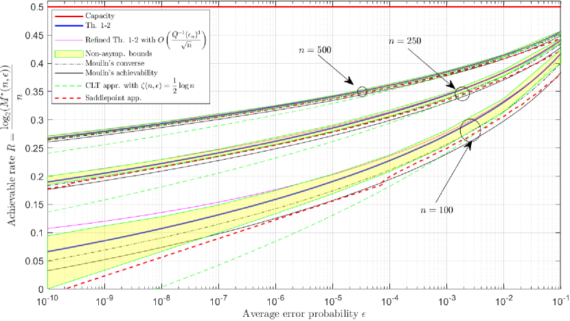
Figure 1: The expansion from Theorems 1 and 3, excluding the $O(\cdot)$ terms, are shown for the BSC(0.11) with $\epsilon\in[10^{-10},10^{-1}]$ and $n=\{100,250,500\}$. The upper and lower boundaries of the shaded region correspond to the non-asymptotic bounds in [3, Th. 33 and 35]; the CLT approximation that takes $\zeta(n,\epsilon)=\frac{1}{2}\log n$, is from [13, Th. 53]; Moulin’s results are (6)–(7); the saddlepoint approximation is from [8, Th. 1] and [9, Sec. III-D].

In [7], Altuğ and Wagner show that in the LD regime, for Gallager-symmetric channels, the prefactors in the lower and upper bounds on the exponentially decaying error probability have the same order; that order depends on whether the channel is singular or nonsingular. Extending the analysis in [15, Sec. III-C-2)] to any Gallager-symmetric channel shows that Gallager-symmetric channels satisfy $A_{0}({P_{X}^{*}})=A_{1}({P_{X}^{*}})=0$, but $\eta({P_{X}^{*}})$ is not necessarily zero (see [15, Sec. III-C-2)] for a counterexample), which means that (61) and (64) are not tight up to the $O(1)$ term for some Gallager-symmetric channels. The findings in [7] suggest that Theorem 1 or Theorem 2 or both could be improved for some channels. The main difference between the achievability bounds in [6, 7] and ours is that [6] bounds the error probability as

$$\epsilon\leq\mathbb{P}\left[\mathcal{D}\right]+(M-1)\mathbb{P}\left[\mathcal{D}^{\mathrm{c}}\cap\{\imath(\overline{\mathbf{X}};\mathbf{Y})\geq\imath(\mathbf{X};\mathbf{Y})\}\right],$$ (68)

where

$$\mathcal{D} \triangleq \left\{\log\frac{P_{Y|X}^{n}(\mathbf{Y}|\mathbf{X})}{Q_{Y}^{n}(\mathbf{Y})}<\tau\right\}$$ (69)

$$Q_{Y}(y) \triangleq c\left(\sum_{x\in\mathcal{X}}P_{X}(x)P_{Y|X}(y|x)^{1/1+\rho}\right)^{1+\rho},\,\,y\in\mathcal{Y}.$$ (70)

Here $Q_{Y}$ is the tilted output distribution, and $\rho\in[0,1]$, $\tau$, and $c$ are some constants. Our achievability bound uses a special case of (70) with $\rho=0$, giving $Q_{Y}=P_{Y}$. Whether the more general bound in (70) yields an improved bound in the MD regime is a question for future work.

III-C Refined Results for Symmetric Channels

Theorem 3 below, refines the achievability and converse results in Theorems 1–2 for Cover–Thomas symmetric channels.

Theorem 3

Let $P_{Y|X}$ be a Cover–Thomas symmetric channel, $V>0$, and $\{\epsilon_{n}\}_{n=1}^{\infty}$ be an SMD sequence (11). Then,

$$\IEEEeqnarraymulticol{3}{l}{\zeta(n,\epsilon_{n})}$$ (71)

$$= \frac{1}{2}\log n+SQ^{-1}(\epsilon_{n})^{2}-\frac{3(\mu_{4}-3V^{2})V-4\mu_{3}^{2}}{72V^{5/2}}\frac{Q^{-1}(\epsilon_{n})^{3}}{\sqrt{n}}$$

$$+O\left(\frac{Q^{-1}(\epsilon_{n})^{4}}{n}\right)+O\left(1\right),$$

where $V$ and $S$ are the $\epsilon$-dispersion (43) and skewness (66) under the uniform input distribution ${P_{X}^{*}}$, and $\mu_{k}=\mathbb{E}\left[(\imath(X;Y)-C)^{k}\right]$ is the $k$-th central moment of the information density under $X\sim{P_{X}^{*}}$.

Proof:

See Appendix F. ∎

III-D Gaussian Channel

The output of the memoryless Gaussian channel in response to the input $\mathbf{X}\in\mathbb{R}^{n}$ is

$$\mathbf{Y}=\mathbf{X}+\mathbf{Z},$$ (72)

where the entries of $\mathbf{Z}$ are drawn i.i.d. from $\mathcal{N}(0,1)$, independent of $\mathbf{X}$. The capacity and dispersion of the Gaussian channel are given by

$$C(P) \triangleq\frac{1}{2}\log(1+P)$$ (73)

$$V(P) \triangleq\frac{P(P+2)}{2(1+P)^{2}}.$$ (74)

In addition to the average error probability constraint (37), an $(n,M,\epsilon,P)$ code for the Gaussian channel with a maximal power constraint requires that each codeword has power $nP$ exactly, i.e.,

$$\left\lVert\mathsf{f}(m)\right\rVert_{2}^{2}\leq nP,\quad\forall\,m\in[M].$$ (75)

The maximum achievable message set size $M^{*}(n,\epsilon,P)$ is defined similarly to (38); the corresponding non-Gaussianity is defined as

$$\zeta(n,\epsilon,P) \triangleq\log M^{*}(n,\epsilon,P)-(nC(P)-\sqrt{nV(P)}Q^{-1}(\epsilon)).$$ (76)

Theorem 4, below, gives lower and upper bounds on the non-Gaussianity $\zeta(n,\epsilon,P)$ in the CLT regime.

Theorem 4

Fix $\epsilon\in(0,1)$ and $P>0$. Then,

$$\zeta(n,\epsilon,P) \geq\frac{1}{2}\log n+S(P)Q^{-1}(\epsilon)^{2}+\underline{B}(P)+O\left(\frac{1}{\sqrt{n}}\right)$$ (77)

$$\zeta(n,\epsilon,P) \leq\frac{1}{2}\log n+S(P)Q^{-1}(\epsilon)^{2}+\overline{B}(P)+O\left(\frac{1}{\sqrt{n}}\right),$$ (78)

where

$$S(P) =\frac{6+6P+4P^{2}+P^{3}}{6(1+P)^{2}(2+P)}$$ (79)

$$\overline{B}(P) =\frac{9P+14P^{2}+5P^{3}}{6(1+P)^{2}(2+P)}+\frac{1}{2}\log\left(\frac{2\pi P}{1+P}\right)$$ (80)

$$\underline{B}(P) =\overline{B}(P)-1-C(P)$$ (81)

Proof:

See Appendix G. ∎

In Fig. 2, the skewness approximations in Theorem 4 are compared with the non-asymptotic bounds and LD approximations from [10], and the CLT approximation from [16]. For the shown $(n,\epsilon,P)$ triples, our skewness approximation (78) is the closest to the non-asymptotic converse bound; our skewness approximation (77) is the closest to the non-asymptotic achievability bound for $\epsilon\gtrapprox 10^{-4}$ while for $\epsilon\lessapprox 10^{-4}$, Shannon’s LD approximation becomes the closest.

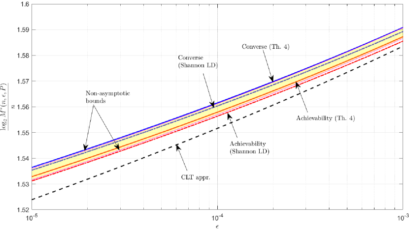
Figure 2: The expansions from Theorem 4, excluding the $O(\cdot)$ term, are shown for the Gaussian channel with $P=10$, $n=400$, and $\epsilon\in[10^{-5},10^{-3}]$. The upper and lower ends of the shaded region correspond to the non-asymptotic bounds from [10, eq. (20)]. Shannon’s LD approximations are from [10, eq. (4)-(5)]; the CLT approximation that takes $\zeta(n,\epsilon,P)=\frac{1}{2}\log n$ is from [16].

Some remarks on Theorem 4 are given in order.

1. Although the bounds in Theorem 4 are only for the CLT regime but not the MD regime, they yield the channel skewness of the Gaussian channel as $S(P)$ since the channel skewness (10) is defined as the coefficient of the $Q^{-1}(\epsilon)^{2}$ term in the non-Gaussianity as $\epsilon\to 0$, and since the lower and upper bounds on the $Q^{-1}(\epsilon)^{2}$ term in (77)–(78) match.

2. The lower bound is derived by analyzing Shannon’s random coding bound [10, eq. 5] in the CLT regime, which draws codewords uniformly over the sphere of radius $\sqrt{nP}$ and employs maximum likelihood decoder. The proof technique is slightly different than the bound (68) that we use for DMCs; we replace the auxiliary event $\mathcal{D}$ in (69) with $Q_{Y}=P_{Y}$ by the event

   $$\mathcal{D}=\{\langle\mathbf{X},\mathbf{Y}\rangle<\tau_{n}\}.$$ (82)

   In the prior tightest CLT approximation for the Gaussian channel, Tan and Tomamichel [16] use (69) to show that $\zeta(n,\epsilon,P)\geq\frac{1}{2}\log n+O(1)$. It turns out that changing (69) to (82) is crucial in deriving the tight lower bound on the channel skewness for the Gaussian channel.

3. The converse bound (78) analyzes Shannon’s sphere-packing bound [10, eq. 15], which is quite different than our method in Theorem 2 for DMCs. Shannon’s sphere-packing converse turns out to be Polyanskiy’s meta-converse [3, Th. 28] applied with the optimal auxiliary output distribution [32, Sec. VI-F], that is, after transforming the channel output $\mathbf{Y}$ to $\mathbf{Y}/\left\lVert\mathbf{Y}\right\rVert_{2}$, the uniform distribution over the $n$-dimensional unit sphere achieves the minimax in [3, Th. 28], and Shannon’s converse bound is equal to that minimax bound. The prior tightest CLT approximation in the converse direction applies the meta-converse bound with the auxiliary output distribution $Q_{Y}^{(n)}=\mathcal{N}(\mathbf{0},(1+P)\mathsf{I}_{n})$, and derives $\zeta(n,\epsilon,P)\leq\frac{1}{2}\log n+O(1)$. This technique turns out to be insufficiently sharp to derive the sharp bound on the channel skewness.

4. In both of achievability and converse bounds, the quantile function of a noncentral $t$-distribution is needed. Since the noncentral $t$-distribution is not a sum of independent random variables, Theorem 6 below, which is for the MD regime, does not apply. Instead, we use the Cornish-Fisher expansion of that distribution, which is available in the CLT regime. Based on the fact that the Cornish-Fisher expansions in general have the same skewness term for the CLT and MD regimes (see Lemma 1, below), we conjecture that the bounds in Theorem 4 hold in the MD regime up to the $S(P)Q^{-1}(\epsilon)^{2}$ term. The question that whether this is true is left to future work.

5. The converse proof first considers the codes such that all codewords have the same power, $nP$, and then uses the relationship [3, Lemma 39]

   $$M(n,\epsilon,P)_{\mathrm{eq}}\leq M(n,\epsilon,P)\leq M(n+1,\epsilon,P)_{\mathrm{eq}},$$ (83)

   where $M(n,\epsilon,P)_{\mathrm{eq}}$ is the maximum achievable message set size, where all codewords have equal powers. The bound in (83) is also shown by Shannon [10]. Let

   $$\overline{B}(P)_{\mathrm{eq}} \triangleq\overline{B}(P)-C(P)$$ (84)

   $$\underline{B}(P)_{\mathrm{eq}} \triangleq\underline{B}(P),$$ (85)

   giving $\overline{B}(P)_{\mathrm{eq}}-\underline{B}(P)_{\mathrm{eq}}=1$. For codes with equal power codewords, Theorem 4 holds with $\overline{B}$ and $\underline{B}$ are replaced by the corresponding constants in (84)–(85). This extends the observation of Moulin [15] applicable to a class of symmetric DMCs with non-lattice information density, to the Gaussian channel with equal power constraint; the gap between the constant terms in the lower and upper bounds on the non-Gaussianity is also 1 nat.

III-E Refined Asymptotics of BHT

We introduce binary hypothesis tests, which play a fundamental role in many coding theorems in the literature.

Let $P$ and $Q$ be two distributions on a common alphabet $\mathcal{X}$. Consider the binary hypothesis test

$$H_{0} \colon X\sim P$$ (86)

$$H_{1} \colon X\sim Q.$$ (87)

A randomized test between those two distributions is defined by a probability transition kernel $P_{W|X}\colon\mathcal{X}\to\{0,1\}$, where $0$ indicates that the test chooses $H_{0}$, i.e., $P$, and $1$ indicates that the test chooses $H_{1}$, i.e., $Q$. We define the minimum achievable type-II error compatible with the type-I error bounded by $1-\alpha$ as [3, eq. (100)]

$$\beta_{\alpha}(P,Q)\triangleq\min\limits_{P_{W|X}\colon\mathbb{P}\left[W=0|H_{0}\right]\geq\alpha}\mathbb{P}\left[W=0|H_{1}\right].$$ (88)

The minimum in (88) is achieved by test given in the Neyman-Pearson Lemma (e.g., [3, Lemma 57]), i.e.,

$$P_{W|X}(0|x)=\begin{cases}1\quad&\text{if }z_{x}>\gamma\\ \tau\quad&\text{if }z_{x}=\gamma\\ 0\quad&\text{if }z_{x}<\gamma\end{cases},$$ (89)

where $z_{x}\triangleq\log\frac{dP}{dQ}(x)$ is the log-likelihood ratio, $\frac{dP}{dQ}$ denotes the Radon-Nikodym derivative, and $\tau$ and $\gamma$ are chosen so that $\alpha=\mathbb{P}\left[W=0|H_{0}\right]$.

Let $P^{(n)}=\prod_{i=1}^{n}P_{i}$ and $Q^{(n)}=\prod_{i=1}^{n}Q_{i}$, where $P_{i}$ and $Q_{i}$ are distributions on a common alphabet $\mathcal{X}$. Theorem 5, below, gives refined asymptotics of $\beta_{\alpha}(P^{(n)},Q^{(n)})$ in the SMD regime.

Define $Z_{i}\triangleq\log\frac{dP_{i}}{dQ_{i}}(X_{i})$, where $X_{i}\sim P_{i}$ for $i\in[n]$, and

$$D_{i} \triangleq\mathbb{E}\left[Z_{i}\right]=D(P_{i}\|Q_{i})$$ (90)

$$V_{i} \triangleq\mathrm{Var}\left[Z_{i}\right]=V(P_{i}\|Q_{i})$$ (91)

$$\mu_{k,i} \triangleq\mathbb{E}\left[(Z_{i}-D_{i})^{k}\right],\quad k\geq 3$$ (92)

$${\mathrm{Sk}}_{i} \triangleq{\mathrm{Sk}}(P_{i}\|Q_{i})=\frac{\mu_{3,i}}{V_{i}^{3/2}}$$ (93)

for $i\in[n]$. Define $\overline{Z}_{i}\triangleq\log\frac{dP_{i}}{dQ_{i}}(\overline{X}_{i})$, where $\overline{X}_{i}\sim Q_{i}$ for $i\in[n]$, and the cumulant generating function of $\overline{Z}_{i}$

$$\kappa_{i}(s) \triangleq\log\mathbb{E}\left[\exp\{s\overline{Z}_{i}\}\right],\quad i\in[n].$$ (94)

Let

$$D \triangleq\frac{1}{n}\sum_{i=1}^{n}D_{i}\quad\quad V\triangleq\frac{1}{n}\sum_{i=1}^{n}V_{i}$$ (95)

$${\mathrm{Sk}} \triangleq\frac{1}{n}\sum_{i=1}^{n}{\mathrm{Sk}}_{i}\quad\quad\mu_{k}\triangleq\frac{1}{n}\sum_{i=1}^{n}\mu_{k,i},\,k\geq 3,$$ (96)

$$\kappa(s) \triangleq\frac{1}{n}\sum_{i=1}^{n}\kappa_{i}(s).$$ (97)

Theorem 5

Let $P_{i}$, $Q_{i}$ be distributions on a common alphabet $\mathcal{X}$, and let $P_{i}$ be absolutely continuous with respect to $Q_{i}$ for $i\in[n]$. Let $\{\epsilon_{n}\}_{n=1}^{\infty}$ be an SMD sequence (11). Assume that

1. $Z_{i}$ satisfies Cramér’s condition for $i\in[n]$, i.e., $\mathbb{E}\left[\exp\{sZ_{i}\}\right]<\infty$ for $s\in\mathbb{R}$ in the neighborhood of 0;

2. $V>0$;

3. there exist positive constants $\beta_{0}$, $\beta_{1}$, and $c>1$ such that $\beta_{0}<|\kappa(s)|<\beta_{1}$ for all $s\in\mathcal{D}\triangleq\{s^{\prime}\in\mathbb{R}\colon|s^{\prime}|<c\}$, and that $\kappa(s)$ is analytic in $\mathcal{D}$;

4. if the sum $\sum_{i=1}^{n}\overline{Z}_{i}$ is non-lattice, then there exist a finite integer $\ell$, a sequence $\{w_{n}\}_{n=1}^{\infty}$ satisfying $\frac{w_{n}}{\log n}\to\infty$, and non-overlapping index sets $\mathcal{I}_{1},\mathcal{I}_{2},\dots,\mathcal{I}_{w_{n}}\subset[n]$, each having size $\ell$, such that

   $$\sum_{i\in\mathcal{I}_{j}}\overline{Z}_{i}\text{ is non-lattice for }j\in[w_{n}].$$ (98)

Then, it holds that

$$-\log\beta_{1-\epsilon_{n}}(P^{(n)},Q^{(n)})$$

$$=nD-\sqrt{nV}Q^{-1}(\epsilon_{n})+\frac{1}{2}\log n+\left(\frac{{\mathrm{Sk}}\sqrt{V}}{6}+\frac{1}{2}\right)Q^{-1}(\epsilon_{n})^{2}$$

$$\quad-\frac{3(\mu_{4}-3V^{2})V-4\mu_{3}^{2}}{72V^{5/2}}\frac{Q^{-1}(\epsilon_{n})^{3}}{\sqrt{n}}$$

$$\quad+O\left(\frac{Q^{-1}(\epsilon_{n})^{4}}{n}\right)+O\left(1\right).$$ (99)

Proof:

See Appendix E. ∎

In Fig. 3 below, we compare the asymptotic expansion in Theorem 5 with the true values from the Neyman-Pearson lemma, the CLT approximation from [3], and the LD approximation from [22] for BHT between two i.i.d. Bernoulli distributions. The first three terms on the right-hand side of (99) constitute the CLT approximation of BHT, and are shown in [3, Lemma 58] in the CLT regime. The coefficient of $Q^{-1}(\epsilon_{n})^{2}$ in the fourth term of (99) is the skewness for BHT. The fifth term in (99) gives the fourth-order characteristic of BHT. A direct application of Theorem 5 to the meta-converse bound [3, Th. 27] shows the converse part of Theorem 3. Together with the achievability part of Theorem 3, this implies that the fourth-order characteristic of Cover–Thomas channels and BHT are the same in the sense that $C,V,S$, and $\mu_{4}$ in Theorem 3 are the same as $D,V,\frac{{\mathrm{Sk}}\sqrt{V}}{6}+\frac{1}{2}$, and $\mu_{4}$ in (99) evaluated at $P^{(n)}=P_{Y|X=x}^{n}$ and $Q^{(n)}=(Q_{Y}^{*})^{n}$, where $x\in\mathcal{X}$ is arbitrary, and $Q_{Y}^{*}$ is the capacity-achieving output distribution.

In Theorem 5, conditions (A) and (B) are used to apply the MD result Lemma 1 (see Section IV-B below) to the sum $\sum_{i=1}^{n}Z_{i}$; conditions (C) and (D) are used to satisfy the conditions of the LD results (Theorems 7 and 8 in Section IV-C below) for the random variable $\sum_{i=1}^{n}\overline{Z}_{i}$. Note that if $\sum_{i=1}^{n}\overline{Z}_{i}$ is lattice, then each of the random variables $\overline{Z}_{i}$, $i\in[n]$ is lattice. In the non-lattice case, the sum $\sum_{i=1}^{n}\overline{Z}_{i}$ can be non-lattice even if one of more of the $\overline{Z}_{i}$ is lattice. Condition (D) of Theorem 5 requires that there are $w_{n}\gg\log n$ non-overlapping, non-lattice partial sums of $\overline{Z}^{n}$, where each partial sum is a sum of $\ell$ random variables. A condition similar to condition (D) with $\ell\leq 2$ is introduced in [15, Def. 15] for the same purpose.

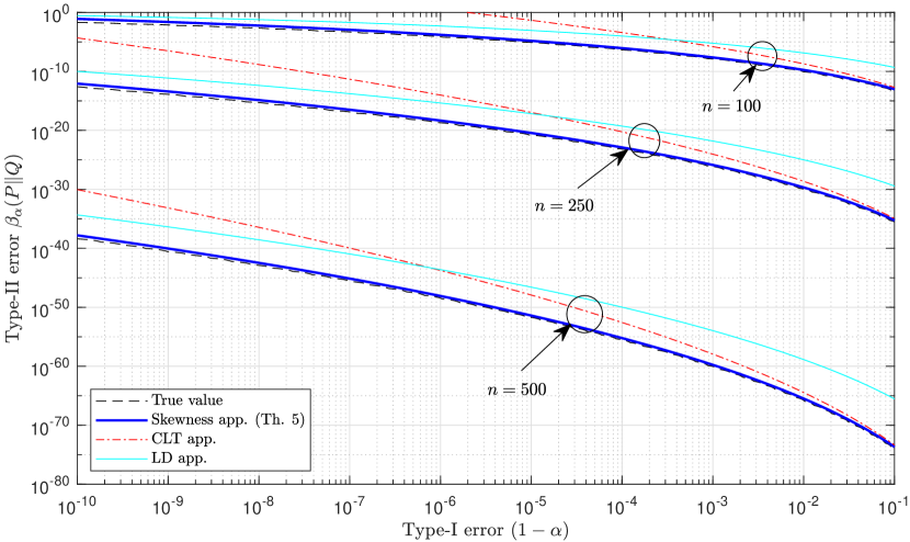
Figure 3: The expansion from Theorem 5, excluding the $O(\cdot)$ terms, is shown for $P_{i}=\mathrm{Bern}(0.6)$, $Q_{i}=\mathrm{Bern}(0.2)$, $i=1,\dots,n$, $n\in\{100,250,500\}$. Our skewness approximation is compared with the true values obtained by the Neyman-Pearson lemma, the CLT approximation from [3, Lemma 58], which consists of the terms up to $\frac{1}{2}\log n$, and the first-order LD approximation from [22, Th. 11.7.1].

IV Proofs of Theorems 1 and 2

We begin by giving the preliminary definitions for quantities related to the moments of a random variable $X$.

IV-A Moment and Cumulant Generating Functions

Below, we dedicate the letters $s$ and $t$ to real scalars and $z$ to complex scalars. The moment generating function (mgf) of $X$ is defined as

$$\phi(z)\triangleq\mathbb{E}\left[\exp\{zX\}\right],\quad z\in\mathbb{C}.$$ (100)

The $j$-th central moment is denoted by

$$\mu_{j}\triangleq\mathbb{E}\left[(X-\mathbb{E}\left[X\right])^{j}\right].$$ (101)

The cumulant generating function (cgf) of $X$ is defined as

$$\kappa(z)\triangleq\log\phi(z)=\sum_{j=1}^{\infty}\kappa_{j}\frac{z^{j}}{j!},$$ (102)

where $\kappa_{j}$ is called the $j$-th cumulant of $X$, and there exists a one-to-one relationship between $\kappa_{j}$ and the central moments up to the order $j$. For example,

$$\kappa_{1} =\mathbb{E}\left[X\right]$$ (103)

$$\kappa_{2} =\mu_{2}$$ (104)

$$\kappa_{3} =\mu_{3}$$ (105)

$$\kappa_{4} =\mu_{4}-3\mu_{2}^{2}.$$ (106)

We use $\phi^{(X)}(\cdot)$ and $\kappa^{(X)}(\cdot)$ to denote the mgf and cgf of $X$ when the random variable is not clear from context. It is straightforward to see that the $j$-th cumulant of $cX$ is given by $\kappa_{j}^{(cX)}=c^{j}\kappa_{j}^{(X)}$, and the cgf of $X+Y$, where $X$ and $Y$ are independent, is

$$\kappa^{(X+Y)}(z)=\kappa^{(X)}(z)+\kappa^{(Y)}(z).$$ (107)

The mgf and cgf are naturally extended to $d$-dimensional random vectors. Let $\mathbf{S}$ be a $d$-dimensional random vector. The mgf and cgf of $\mathbf{S}$ are denoted by

$$\phi(\mathbf{z}) \triangleq\mathbb{E}\left[\exp\{\langle\mathbf{z},\mathbf{S}\rangle\}\right],\quad\mathbf{z}\in\mathbb{C}^{d},$$ (108)

$$\kappa(\mathbf{z}) \triangleq\log\phi(\mathbf{z}).$$ (109)

Next, we present the supporting results used to bound the probability terms that appear in the proofs of Theorems 1 and 2.

IV-B MD Asymptotics

Theorem 6, stated next, is an MD result that bounds the probability that the sum of $n$ i.i.d. random variables normalized by a factor $\frac{1}{\sqrt{n}}$ deviates from the mean by $o(\sqrt{n})$. The resulting probability is an SMD sequence (11).

Theorem 6 (Petrov [29, Ch. 8, Th.  4])

Let $X_{1},\dots,X_{n}$ be independent random variables. Let $\mathbb{E}\left[X_{i}\right]=0$ for $i=1,\dots,n$, $\kappa_{j}=\frac{1}{n}\sum_{i=1}^{n}\kappa_{j}^{(X_{i})}$ for $j\geq 2$, and ${\mathrm{Sk}}=\frac{\kappa_{3}}{\kappa_{2}^{3/2}}$. Define

$$S_{n} \triangleq\frac{1}{\sqrt{n\kappa_{2}}}\sum_{i=1}^{n}X_{i}$$ (110)

$$F_{n}(x) \triangleq\mathbb{P}\left[S_{n}\leq x\right].$$ (111)

Suppose that there exist some positive constants $t_{0}$ and $H$ such that the mgf satisfies

$$\phi^{(X_{i})}(t)<H$$ (112)

for all $|t|\leq t_{0}$ and $i=1,\dots,n$. This condition is called Cramér’s condition. Let $x>0$ and $x=o(\sqrt{n})$. Then, it holds that

$$1-F_{n}(x)=Q(x)\exp\left\{\frac{x^{3}}{\sqrt{n}}\lambda_{n}\left(\frac{x}{\sqrt{n}}\right)\right\}\left(1+O\left(\frac{1+x}{\sqrt{n}}\right)\right)$$ (113)

$$F_{n}(-x)=Q(x)\exp\left\{\frac{-x^{3}}{\sqrt{n}}\lambda_{n}\left(\frac{-x}{\sqrt{n}}\right)\right\}\left(1+O\left(\frac{1+x}{\sqrt{n}}\right)\right),$$ (114)

where

$$\lambda_{n}(x)\triangleq\sum_{i=0}^{\infty}a_{i}x^{i}$$ (115)

is Cramér’s series whose first two coefficients are

$$a_{0} =\frac{{\mathrm{Sk}}}{6}$$ (116)

$$a_{1} =\frac{\kappa_{4}\kappa_{2}-3\kappa_{3}^{2}}{24\kappa_{2}^{3}}.$$ (117)

The $O(\cdot)$ terms in (113)–(114) constitute a bottleneck in deriving the $O(1)$ terms in (61) and (64), that is, one needs to compute the leading term of the $O(\cdot)$ terms in (113)–(114) in order to compute the $O(1)$ terms in our achievability and converse bounds.

Inverting Theorem 6, namely, obtaining an expansion for $x$ in terms $y$ where $F_{n}(-x)=Q(y)$, is advantageous in many applications. For $Q(y)=\epsilon_{n}$, where $\{\epsilon_{n}\}_{n=1}^{\infty}$ is an SMD sequence of probabilities (11), Lemma 1, below, gives the corresponding sequence of quantiles. In the CLT regime, in which $F_{n}(-x)\in(0,1)$ is equal to a value independent of $n$, that expansion is known as the Corner-Fisher theorem [33], which inverts the Edgeworth expansion.

Lemma 1

Let $X_{1},\dots,X_{n}$ satisfy the conditions in Theorem 6. Let $y\triangleq Q^{-1}(\epsilon_{n})=o(\sqrt{n})$. Suppose that $F_{n}(-x)=Q(y)=\epsilon_{n}$, then

$$x=y-\frac{b_{0}y^{2}}{\sqrt{n}}+\frac{b_{1}y^{3}}{n}+O\left(\frac{y^{4}}{n^{3/2}}\right)+O\left(\frac{1}{\sqrt{n}}\right),$$ (118)

where

$$b_{0} \triangleq\frac{{\mathrm{Sk}}}{6}$$ (119)

$$b_{1} \triangleq\frac{3\kappa_{4}\kappa_{2}-4\kappa_{3}^{2}}{72\kappa_{2}^{3}}.$$ (120)

Proof:

See Appendix A. ∎

A weaker version of Lemma 1 with only the first two terms in (118), and with $\epsilon_{n}$ decaying polynomially with $n$ is proved in [20, Lemma 7]. We use Theorem 6 and Lemma 1 to bound the probability $\mathbb{P}\left[\imath(\mathbf{X};\mathbf{Y})\leq\tau\right]$, where $\tau$ is a threshold satisfying the condition in Theorem 6, and the resulting probability is an SMD sequence (11). Although the MD approximation to the cdf of the normalized sum in Theorem 6 is seemingly different than the CLT approximation to the same cdf (the Edgeworth expansion), their inverted theorems, i.e., Lemma 1 and the Cornish-Fisher theorem [33], respectively, have similar forms; for the continuous random variables, the Cornish-Fisher theorem admits the formula in (118), where $O\left(\frac{1}{\sqrt{n}}\right)$ is replaced by $\frac{b_{0}}{\sqrt{n}}+O\left(\frac{1}{n}\right)$. This is the main reason why the channel skewness bounds computed in the CLT regime extend to the MD regime without change.

IV-C Strong LD Asymptotics

For the results in this section, we consider a sequence of $d$-dimensional random vectors $\mathbf{S}_{n}=(S_{n,1},\dots,S_{n,d})$, $n=1,2,\dots$. Let $\phi_{n}(\cdot)$ denote the mgf of $\mathbf{S}_{n}$, and let $\kappa_{n}(\cdot)$ be the normalized cgf of $\mathbf{S}_{n}$ denoted by

$$\phi_{n}(\mathbf{z}) \triangleq\phi^{(\mathbf{S}_{n})}(\mathbf{z})$$ (121)

$$\kappa_{n}(\mathbf{z}) \triangleq\frac{1}{n}\log\phi_{n}(\mathbf{z}).$$ (122)

The Fenchel–Legendre transform of $\kappa_{n}(\cdot)$ is given by

$$\Lambda_{n}(\mathbf{x})\triangleq\sup_{\mathbf{t}\in\mathbb{R}^{d}}\left\{\langle\mathbf{t},\mathbf{x}\rangle-\kappa_{n}(\mathbf{t})\right\},$$ (123)

where $\mathbf{x}\in\mathbb{R}^{d}$. The quantity (123) is commonly known as the rate function in the LD literature [34, Ch. 2.2].

Theorem 7, below, is a strong LD result for an arbitrary sequence of random vectors $\mathbf{S}_{n}$ in $\mathbb{R}^{d}$; here, strong refers to characterizing the exact prefactor in front of the LD exponent.

Theorem 7 (Chaganty and Sethuraman [30, Th. 3.4])

Let $\{\mathbf{a}_{n}\}_{n=1}^{\infty}$ be a bounded sequence of $d$-dimensional vectors. Assume that the following conditions hold.
Smoothness (S): $\kappa_{n}(\mathbf{z})$ is bounded below and above, and is analytic in $\mathcal{D}^{d}$, where $\mathcal{D}\triangleq\{\mathbf{z}\in\mathbb{C}\colon|\mathbf{z}|<c\}$ and $c$ is a finite constant;
Non-Degenerate (ND): there exist a real sequence $\{\mathbf{s}_{n}\}_{n=1}^{\infty}$ and constants $c_{0}$ and $c_{1}$ that satisfy

$$\nabla\kappa_{n}(\mathbf{s}_{n})=\mathbf{a}_{n}$$ (124)

$$0<c_{0}<s_{n,j}<c_{1}<c\text{ for all }j\in[d]\text{ and }n\geq 1,$$ (125)

where $c$ is the constant given in condition (S), and the Hessian matrix $\nabla^{2}\kappa_{n}(\mathbf{s}_{n})$, which is a covariance matrix of a tilted distribution obtained from $\mathbf{S}_{n}$, is positive definite with a minimum eigenvalue bounded away from zero for all $n$;
Non-Lattice (NL): there exists $\delta_{0}>0$ such that for any given $\delta_{1}$ and $\delta_{2}$ such that $0<\delta_{1}<\delta_{0}<\delta_{2}$

$$\sup_{\mathbf{t}\colon\delta_{1}<\|\mathbf{t}\|_{\infty}\leq\delta_{2}}\left\lvert\frac{\phi_{n}(\mathbf{s}_{n}+\mathrm{i}\mathbf{t})}{\phi_{n}(\mathbf{s}_{n})}\right\rvert=o\left(n^{-d/2}\right),$$ (126)

where $\mathrm{i}=\sqrt{-1}$ is the imaginary unit. Then,

$$\mathbb{P}\left[\mathbf{S}_{n}\geq n\mathbf{a}_{n}\right]=\frac{E_{\mathrm{NL}}}{n^{d/2}}\exp\{-n\Lambda_{n}(\mathbf{a}_{n})\}(1+o(1)),$$ (127)

where

$$E_{\mathrm{NL}}\triangleq\frac{1}{(2\pi)^{d/2}\left(\prod\limits_{j=1}^{d}s_{n,j}\right)\sqrt{\det(\nabla^{2}\kappa_{n}(\mathbf{s}_{n}))}}.$$ (128)

Condition (S) of Theorem 7 is a smoothness assumption for the cgf $\kappa_{n}$, which is a generalization of Cramér’s condition that appears in the LD theorem for the sum of i.i.d. random vectors [34, Th. 2.2.30]. Condition (S) implies that all moments of the tilted distribution obtained from $\mathbf{S}_{n}$ are finite. Condition (ND) is used to ensure that $\mathbf{S}_{n}$ is a non-degenerate random vector, meaning that it does not converge in distribution to a random vector with $\ell<d$ dimensions, and that the rate function $\Lambda_{n}(\mathbf{a}_{n})$ is bounded and does not decay to zero. The latter follows from the boundedness condition in (125), and implies that the probability of interest is in the LD regime. The ratio $\frac{\phi_{n}(\mathbf{s}_{n}+\mathrm{i}\mathbf{t})}{\phi_{n}(\mathbf{s}_{n})}$ in (126) is equal to the characteristic function of a random vector that is obtained by tilting $\mathbf{S}_{n}$ by $\mathbf{s}_{n}$ [30]. A random variable is non-lattice if and only if its characteristic function satisfies $|\phi(\mathsf{i}t)|<1$ for all real $t\neq 0$ [35, Ch. XV, Sec. 1, Lemma 4]. Therefore, since tilting does not affect the support of a distribution, condition (NL) requires $\mathbf{S}_{n}$ to be a non-lattice random vector. Condition (NL) is used to guarantee that the absolute value of that characteristic function decays to zero quickly enough outside a neighborhood of the origin, which makes the random vector $\mathbf{S}_{n}$ behave like a sum of $n$ non-lattice random vectors.

Let $\overline{\mathbf{X}}$ be a random codeword that is independent of both the transmitted codeword $\mathbf{X}$ and the channel output $\mathbf{Y}$. If $\imath(\mathbf{X};\mathbf{Y})$ and $\imath(\overline{\mathbf{X}};\mathbf{Y})$ are non-lattice, we apply Theorem 7 to the sequence of 2-dimensional non-lattice random vectors $(\imath(\mathbf{X};\mathbf{Y}),\imath(\overline{\mathbf{X}};\mathbf{Y})-\imath(\mathbf{X};\mathbf{Y}))$ to bound the probability $\mathbb{P}\left[\imath(\overline{\mathbf{X}};\mathbf{Y}))\geq\imath(\mathbf{X};\mathbf{Y})\geq\tau_{n}\right]$ for some sequence $\tau_{n}$.

When applied to the sum of $n$ i.i.d. random variables $\mathbf{S}_{n}=\sum_{i=1}^{n}\mathbf{A}_{i}$, $\kappa_{n}$ in (122) reduces to the cgf of $\mathbf{A}_{1}$ as

$$\kappa(\mathbf{z})=\log\mathbb{E}\left[\exp\{\langle\mathbf{z},\mathbf{A}_{1}\rangle\}\right].$$ (129)

In our application, since $\mathbf{A}_{1}=(\imath(X_{1};Y_{1}),\imath(\overline{X}_{1};Y_{1})-\imath(X_{1};Y_{1}))$ has a finite support, the expectation in (129) is bounded, and all moments of $\mathbf{A}_{1}$ are finite; therefore, condition (S) of Theorem 7 is satisfied. Further, the characteristic function of the sum of $n$ i.i.d. random vectors is equal to $n$-th power of the characteristic function of one of the summands. Therefore, the left-hand side of (126) decays to zero exponentially fast for the sum of i.i.d. non-lattice random vectors, satisfying condition (NL) of Theorem 7 with room to spare.

We use the following strong LD result to bound the probability $\mathbb{P}\left[\imath(\overline{\mathbf{X}};\mathbf{Y}))\geq\imath(\mathbf{X};\mathbf{Y})\geq\tau_{n}\right]$ with lattice $\imath(\mathbf{X};\mathbf{Y})$ and $\imath(\overline{\mathbf{X}};\mathbf{Y})$.

Theorem 8

Suppose that $\mathbf{S}_{n}=(S_{n,1},\dots,S_{n,d})$, and $S_{n,j}$ is a lattice random variable with span $h_{n,j}$, i.e., $\mathbb{P}\left[S_{n,j}\in\{b_{n,j}+kh_{n,j}\colon k\in\mathbb{Z}\}\right]=1$ for some $b_{n,j}$, such that there exist positive constants $\underline{h}_{j}$ and $\overline{h}_{j}$ satisfying $\underline{h}_{j}<h_{n,j}<\overline{h}_{j}$ for all $j\in[d]$, $n\geq 1$. Assume that conditions (S) and (ND) in Theorem 7 hold, and replace condition (NL) by
Lattice (L): there exists $\bm{\lambda}>\bm{0}$ such that for any given $\bm{\delta}$ satisfying $\bm{0}<\bm{\delta}<\bm{\lambda}$,

$$\sup_{\mathbf{t}\colon\delta_{j}<|t_{j}|\leq\frac{\pi}{h_{n,j}}\text{ for }j\in[d]}\left\lvert\frac{\phi_{n}(\mathbf{s}_{n}+\mathrm{i}\mathbf{t})}{\phi_{n}(\mathbf{s}_{n})}\right\rvert=o\left(n^{-d/2}\right).$$ (130)

Assume that $n\mathbf{a}_{n}$ is in the range of the random vector $\mathbf{S}_{n}$. Then,

$$\mathbb{P}\left[\mathbf{S}_{n}\geq n\mathbf{a}_{n}\right]=\frac{E_{\mathrm{L}}}{n^{d/2}}\exp\{-n\Lambda_{n}(\mathbf{a}_{n})\}(1+o(1)),$$ (131)

where

$$E_{\mathrm{L}}\triangleq\frac{1}{(2\pi)^{d/2}\sqrt{\det(\nabla^{2}\kappa_{n}(\mathbf{s}_{n}))}}\left(\prod\limits_{j=1}^{d}\frac{h_{n,j}}{1-\exp\{-s_{n,j}h_{n,j}\}}\right).$$ (132)

Proof:

The one-dimensional lattice case, i.e., $d=1$, is proved in [36, Th. 3.5]. The proof of the $d$-dimensional lattice case follows by inspecting the proofs for the $d$-dimensional non-lattice random vectors in [30, Th. 3.4] and the one-dimensional lattice random variables in [36, Th. 3.5]. Specifically, in the proof of [30, Th. 3.4], we replace [30, Th. 2.4] by [36, Th. 2.10]. The auxiliary result [36, Th. 2.10] gives the asymptotics of an expectation of a lattice random variable. The modification in the proof yields Theorem 8. ∎

If $\mathbf{S}_{n}=(S_{n,1},\dots,S_{n,d})$ is a sum of $n$ i.i.d. random vectors, where

$$S_{n,j}=\sum_{i=1}^{n}A_{i,j},\quad j\in[d],$$ (133)

and $A_{1,j}$ is a lattice random variable with span $h_{j}$ for $j\in[d]$, then it holds that

$$\sup_{\delta_{j}<|t_{j}|\leq\frac{\pi}{h_{j}}}\left\lvert\frac{\phi^{(X_{1,j})}(s_{j}+\mathrm{i}t_{j})}{\phi^{(X_{1,j})}(s_{j})}\right\rvert<1,\quad j\in[d].$$ (134)

The bound (134) follows from [35, Ch. 15, Sec. 1, Lemma 4] since $\frac{\phi^{(A_{1,j})}(s_{j}+\mathrm{i}t_{j})}{\phi^{(A_{1,j})}(s_{j})}$ is a characteristic function of a lattice random variable with span $h_{j}$. The condition in (130) modifies the condition in (126) for lattice random vectors by considering a single period of that characteristic function. If $\mathbf{S}_{n}$ is an i.i.d. sum, then the left-hand side of (130) decays exponentially with $n$, and condition (L) is satisfied. Note that if $h_{n,j}\to 0$ for all $(n,j)$ pairs, then $\mathbf{S}_{n}$ converges to a non-lattice random vector, and the prefactor $E_{\mathrm{L}}$ converges to the prefactor for the non-lattice random vectors, $E_{\mathrm{NL}}$.

Altuğ and Wagner derive an LD bound in [6, Lemma 3] that applies to the sum of $n$ i.i.d. 2-dimensional random vectors, where each summand can be either non-lattice or lattice. However, their prefactor is worse than both $E_{\mathrm{NL}}$ and $E_{\mathrm{L}}$. Since our achievability proof in Section IV-D relies on only the fact that the prefactor in the LD bound is a bounded constant (see (152), below), [6, Lemma 3] is also applicable in our achievability proof. If one seeks to derive the $O(1)$ term in (61), the tightness of the prefactor used in the probability bound will be important.

IV-D Proof of Theorem 1

The proof consists of two parts, and follows steps similar to the achievability proof in [15]. First, we derive a refined asymptotic achievability bound for an arbitrary input distribution $P_{X}\in\mathcal{P}$. Then, we optimize that achievability bound over all $P_{X}\in\mathcal{P}$.

Lemma 2

Suppose that $\epsilon_{n}$ is an SMD sequence (11). Fix some $P_{X}\in\mathcal{P}$ such that $(P_{X},P_{Y|X})$ is a nonsingular pair and $V_{\mathrm{u}}(P_{X})>0$ for all $n$. It holds that

$$\IEEEeqnarraymulticol{3}{l}{\log M^{*}(n,\epsilon_{n})}$$ (135)

$$\geq nI(P_{X})-\sqrt{nV_{\mathrm{u}}(P_{X})}Q^{-1}(\epsilon_{n})+\frac{1}{2}\log n$$

$$+Q^{-1}(\epsilon_{n})^{2}\bigg{(}\frac{{\mathrm{Sk}}_{\mathrm{u}}(P_{X})\sqrt{V_{\mathrm{u}}(P_{X})}}{6}+\frac{1-\eta(P_{X})}{2(1+\eta(P_{X}))}\bigg{)}$$

$$+O\left(\frac{Q^{-1}(\epsilon_{n})^{3}}{\sqrt{n}}\right)+O(1).$$

We require $V_{\mathrm{u}}(P_{X})>0$ in order to apply Theorems 6–8.

Proof:

We generate $M$ i.i.d. codeword according to the input distribution $P_{X}^{n}$, and employ a maximum likelihood decoder. Let $W$ be the transmitted message that is equiprobably distributed on $[M]$, and let $\hat{W}$ be the decoder output. Define the random variables

$$Z \triangleq\imath(\mathbf{X};\mathbf{Y})$$ (136)

$$\overline{Z} \triangleq\imath(\overline{\mathbf{X}};\mathbf{Y}),$$ (137)

where $(\mathbf{X},\overline{\mathbf{X}},\mathbf{Y})$ is distributed according to $P_{\mathbf{X},\overline{\mathbf{X}},\mathbf{Y}}(\mathbf{x},\overline{\mathbf{x}},\mathbf{y})=P_{X}^{n}(\mathbf{x}^{n})P_{X}^{n}(\overline{\mathbf{x}})P_{Y|X}^{n}(\mathbf{y}|\mathbf{x})$. The random variable $\overline{Z}$ corresponds to the information density obtained from a sample from the random codebook, independent from both $\mathbf{X}$ and the received vector $\mathbf{Y}$.

IV-D1 Error analysis

Fix a threshold value $\tau_{n}$

$$\tau_{n}\triangleq nI(P_{X})-\sqrt{nV_{\mathrm{u}}(P_{X})}t_{n},$$ (138)

where $t_{n}$ will be specified in (145), below. Define the event

$$\mathcal{D}\triangleq\{Z<\tau_{n}\}.$$ (139)

We weaken the RCU bound from [3, Th. 16] and bound the average error probability as

$$\IEEEeqnarraymulticol{3}{l}{\mathbb{P}\left[\hat{W}\neq W\right]}$$ (140)

$$\leq \mathbb{E}\left[\min\left\{1,M-1\,\mathbb{P}\left[\overline{Z}\geq Z|\mathbf{X},\mathbf{Y}\right]\right\}\right]$$

$$\leq \mathbb{P}\left[\mathcal{D}\right]+(M-1)\mathbb{P}\left[\overline{Z}\geq Z\geq\tau_{n}\right].$$ (141)

Define the function

$$h(x)\triangleq\frac{1}{\sqrt{2\pi}}\exp\left\{-\frac{Q^{-1}(x)^{2}}{2}\right\}$$ (142)

and the sequences

$$h_{n} \triangleq\frac{1}{\sqrt{nV_{\mathrm{u}}(P_{X})}}h(\epsilon_{n})$$ (143)

$$\tilde{\epsilon}_{n} \triangleq\epsilon_{n}-h_{n}.$$ (144)

Below, we show that the first and second terms in (141) are bounded by $\tilde{\epsilon}_{n}$ and $h_{n}$, respectively. Here, $h_{n}$ is chosen so that $\log M$ is maximized up to the $O(Q^{-1}(\epsilon_{n})^{2})$ term given that the right-hand side of (141) is equal to $\epsilon_{n}$.

We set $t_{n}$ in (138) as

$$\mathbb{P}\left[\mathcal{D}\right] =\mathbb{P}\left[\frac{Z-nI(P_{X})}{\sqrt{nV_{u}(P_{X})}}\leq-t_{n}\right]=\tilde{\epsilon}_{n}.$$ (145)

Since the channel is a DMC, the random variable $\imath(X;Y)$ has a finite support and is bounded. Therefore, Cramér’s condition in Theorem 6 is satisfied. Applying the MD result in Lemma 1 to (145), we get

$$t_{n} =Q^{-1}(\tilde{\epsilon}_{n})-\frac{{\mathrm{Sk}}_{\mathrm{u}}(P_{X})Q^{-1}(\tilde{\epsilon}_{n})^{2}}{6\sqrt{n}}$$

$$\quad+O\left(\frac{Q^{-1}(\tilde{\epsilon}_{n})^{3}}{n}\right)+O\left(\frac{1}{\sqrt{n}}\right).$$ (146)

We compute the first two derivatives of the $Q^{-1}(x)$ function as

$$(Q^{-1})^{\prime}(x) =\frac{1}{Q^{\prime}(Q^{-1}(x))}=\frac{-1}{h(x)}$$ (147)

$$(Q^{-1})^{\prime\prime}(x) =-\frac{Q^{-1}(x)}{h(x)^{2}}.$$ (148)

By taking the Taylor series expansion of $Q^{-1}(\cdot)$ around $\epsilon_{n}$ and using (146)–(148), we get

$$t_{n} =Q^{-1}(\epsilon_{n})-\frac{{\mathrm{Sk}}_{\mathrm{u}}(P_{X})Q^{-1}({\epsilon}_{n})^{2}}{6\sqrt{n}}$$

$$\quad+O\left(\frac{Q^{-1}(\epsilon_{n})^{3}}{n}\right)+O\left(\frac{1}{\sqrt{n}}\right).$$ (149)

Next, we bound the probability $\mathbb{P}\left[\overline{Z}\geq Z\geq\tau_{n}\right]$. Define the random vector $\mathbf{U}\triangleq(U_{1},U_{2})=(Z,\overline{Z}-Z)$. and the sequence

$$\mathbf{a}_{n}=(a_{n,1},a_{n,2})=\left(\frac{\tau_{n}}{n},0\right).$$ (150)

Applying Theorems 7 or 8 depending on whether $\imath(X;Y)$ is non-lattice or lattice, we get

$$\mathbb{P}\left[\overline{Z}\geq Z\geq\tau_{n}\right] =\mathbb{P}\left[\mathbf{U}\geq n\mathbf{a}_{n}\right]$$ (151)

$$\leq\frac{E}{n}\exp\{-n\Lambda(\mathbf{a}_{n})\}(1+o(1)),$$ (152)

where

$$E =\begin{cases}E_{\mathrm{NL}}&\text{if }\imath(X;Y)\text{ is non-lattice}\\ E_{\mathrm{L}}&\text{if }\imath(X;Y)\text{ is lattice.}\end{cases}$$ (153)

$$\Lambda(\mathbf{a}_{n}) =\sup_{\mathbf{s}_{n}\in\mathbb{R}^{2}}\{\langle\mathbf{a}_{n},\mathbf{s}_{n}\rangle-\kappa(\mathbf{s}_{n})\}$$ (154)

$$\kappa(\mathbf{s}_{n}) =\frac{1}{n}\log\mathbb{E}\left[\exp\{\langle\mathbf{s}_{n},\mathbf{U}\rangle\}\right].$$ (155)

Note that the functions $\kappa(\cdot)$ and $\Lambda(\cdot)$ do not depend on $n$ since $\mathbf{U}$ is an i.i.d. sum. The rate function $\Lambda(\mathbf{a}_{n})$ has the Taylor series expansion

$$\Lambda(\mathbf{a}_{n}) =I(P_{X})+(a_{n,1}-I(P_{X}))+\frac{(a_{n,1}-I(P_{X}))^{2}}{(1+\eta(P_{X}))V_{\mathrm{u}}(P_{X})}$$

$$\quad+O(|a_{n,1}-I(P_{X})|^{3})$$ (156)

$$=a_{n,1}+\frac{1}{n}\frac{Q^{-1}(\epsilon_{n})^{2}}{1+\eta(P_{X})}+O\left(\frac{Q^{-1}(\epsilon_{n})^{3}}{n^{3/2}}\right)+O\left(\frac{1}{n}\right).$$ (157)

In the application of Theorems 7 and 8, conditions (S), (NL), and (L) are already satisfied since $U_{1}$ and $U_{2}$ have finite supports. The verification of condition (ND) and the derivation of (157) appear in Appendix B.

We set

$$\log M =nI(P_{X})-\sqrt{nV_{\mathrm{u}}(P_{X})}Q^{-1}(\epsilon_{n})+\frac{1}{2}\log n$$

$$+Q^{-1}(\epsilon_{n})^{2}\bigg{(}\frac{{\mathrm{Sk}}_{\mathrm{u}}(P_{X})\sqrt{V_{\mathrm{u}}(P_{X})}}{6}+\frac{1-\eta(P_{X})}{2(1+\eta(P_{X}))}\bigg{)}$$

$$+O\left(\frac{Q^{-1}(\epsilon_{n})^{3}}{\sqrt{n}}\right)+O(1).$$ (158)

We put (138) into (149), and then (150) into (152) to bound the probability $\mathbb{P}\left[\overline{Z}\geq Z\geq\tau_{n}\right]$. Then, from the expansion (157), we get

$$M\mathbb{P}\left[\overline{Z}\geq Z\geq\tau_{n}\right]\leq h_{n},$$ (159)

where $h_{n}$ is defined in (143). Combining (141), (145), and (159) completes the proof of Lemma 2. ∎

To complete the proof of Theorem 1, it only remains to maximize the right-hand side of (135) over $P_{X}\in\mathcal{P}$. The following arguments extend the proof of [15, Lemma 9] to the MD regime. Define

$$G(P_{X})\triangleq-\sqrt{V_{\mathrm{u}}(P_{X})}Q^{-1}(\epsilon_{n}).$$ (160)

Let $\mathbf{g}$ be a vector whose components approach zero with a rate $O\left(\frac{Q^{-1}(\epsilon_{n})}{\sqrt{n}}\right)$ satisfying $\mathbf{g}^{\top}\bm{1}=0$, and $f(\mathbf{g})$ be the right-hand side of (135) evaluated at $P_{X}={P_{X}^{*}}+\mathbf{g}\in\mathcal{P}$ for some ${P_{X}^{*}}\in\mathcal{P}^{*}$. We apply the Taylor series expansion to $f(\mathbf{g})$ and get

$$f(\mathbf{g}) \triangleq nI({P_{X}^{*}})+n\mathbf{g}^{\top}\nabla I({P_{X}^{*}})+\frac{n}{2}\mathbf{g}^{\top}\nabla^{2}I({P_{X}^{*}})\mathbf{g}$$

$$\quad+O(n\|\mathbf{g}\|_{\infty}^{3})+\sqrt{n}G({P_{X}^{*}})+\sqrt{n}\mathbf{g}^{\top}\nabla G({P_{X}^{*}})$$

$$\quad+\sqrt{n}O(\|\mathbf{g}\|_{\infty}^{2})+\frac{1}{2}\log n$$

$$\quad+Q^{-1}(\epsilon_{n})^{2}\bigg{(}\frac{{\mathrm{Sk}}_{\mathrm{u}}({P_{X}^{*}})\sqrt{V_{\mathrm{u}}({P_{X}^{*}})}}{6}+\frac{1-\eta({P_{X}^{*}})}{2(1+\eta({P_{X}^{*}}))}\bigg{)}$$

$$\quad+O\left(\frac{Q^{-1}(\epsilon_{n})^{3}}{\sqrt{n}}\right)+O(1)$$ (161)

$$=n\mathbf{g}^{\top}\nabla I({P_{X}^{*}})+\frac{n}{2}\mathbf{g}^{\top}\nabla^{2}I({P_{X}^{*}})\mathbf{g}$$

$$\quad+\sqrt{n}\mathbf{g}^{\top}\nabla G({P_{X}^{*}})+b,$$ (162)

where $b$ is the right-hand side of (135), which is independent of $\mathbf{g}$. From (47) and [5, Th. 4.5.1], for every $\mathbf{g}$ such that ${P_{X}^{*}}+\mathbf{g}$ is a valid probability distribution and $n$ large enough, it holds

$$f(\mathbf{g}) \leq\sup_{\mathbf{g^{\prime}}\in\mathcal{L}}\bigg{\{}-\frac{n}{2}\mathbf{g^{\prime}}^{\top}\mathsf{J}\mathbf{g^{\prime}}+\sqrt{n}\mathbf{g^{\prime}}^{\top}\nabla G({P_{X}^{*}})+b\bigg{\}},$$ (163)

where $\mathsf{J}$ and $\mathcal{L}$ are defined in (49)–(50); and the right-hand side of (163) is achieved by some $\mathbf{g}$ with $g_{x}=0$ for $x\notin\mathcal{X}^{\dagger}$. Since ${P_{X}^{*}}$ is dispersion-achieving, $\mathbf{g}^{\top}\nabla G({P_{X}^{*}})=0$ for any $\mathbf{g}$ in the kernel of $\mathsf{J}$. Therefore, the problem (163) reduces to

$$\sup_{\mathbf{g}\in\mathcal{L}}\mathbf{g}^{\top}\mathbf{h}-\frac{1}{2}\mathbf{g}^{\top}\mathsf{J}\mathbf{g},$$ (164)

where $\mathbf{h}$ is the orthogonal projection of $\frac{\nabla G({P_{X}^{*}})}{\sqrt{n}}$ onto the row space of $\mathsf{J}$. Under the assumption $\mathcal{X}^{\dagger}=\mathcal{X}^{*}$, the supremum in (164) is achieved by

$$\mathbf{g}^{*}=\tilde{\mathsf{J}}\mathbf{h},$$ (165)

where $\tilde{\mathsf{J}}$ is given in (53), and the value of supremum in (164) is $A_{0}({P_{X}^{*}})Q^{-1}(\epsilon_{n})^{2}$. See Appendix C for the details. Combining the values of $b$ and the value of (164) gives the maximum of (135) over all input distributions $P_{X}\in\mathcal{P}$ and completes the proof of Theorem 1.

IV-E Proof of Theorem 2

The proof analyzes Tomamichel and Tan’s non-asymptotic converse bound in [14, Prop. 6] using some techniques from [15, Lemmas 9 and 14].

The main difference between our proof and Moulin’s proof in [15] is that while Moulin analyzes the meta-converse bound [3, Th. 27], we analyze a relaxation of the meta-converse, given in Lemma 4, below. In general, the analysis of the meta-converse is more involved since it requires to split the code into subcodes according to the types of the codewords, and then to carefully combine the bounds for each subcode. The advantage of Lemma 4 over the meta-converse bound is that the optimization problem in Lemma 4 can be converted into a simpler single-letter minimax problem as we show in Lemma 3, and the type-splitting step is avoided. A similar simplification to a single-letter problem using the meta-converse is possible (i) under the average error probability criterion for channels that satisfy certain symmetry conditions [3, Th. 28] (e.g., Cover–Thomas symmetric channels satisfy these symmetry conditions) and (ii) under the maximal error probability criterion for arbitrary DMCs [3, Th. 31]. While both approaches yield the same upper bound $\overline{S}$ on the skewness (in the CLT regime in Moulin’s work and in the MD regime in our work), we note that Lemma 4 is not tight enough to obtain the tightest $O(1)$ term in the converse (64), which we do not focus on here.

We define the divergence spectrum [37, Ch. 4], [14], which gives a lower bound on the minimum type-II error probability of the binary hypothesis test, $\beta_{1-\epsilon}(P,Q)$,

$$D_{s}^{\epsilon}(P\|Q)\triangleq\sup\left\{\gamma\in\mathbb{R}\colon\mathbb{P}\left[\log\frac{P(X)}{Q(X)}\leq\gamma\right]\leq\epsilon\right\},$$ (166)

where $\epsilon\in(0,1)$, $P,Q\in\mathcal{P}$, and $X\sim P$.

The main tools to prove Theorem 2, presented below, are an asymptotic expansion of the divergence spectrum in the MD regime, Lemma 3, and a channel coding converse based on the divergence spectrum, Lemma 4.

Lemma 3

Fix some $\mathbf{x}\in\mathcal{X}^{n}$ and $Q_{Y}\in\mathcal{Q}$. Assume that $\{\epsilon_{n}\}_{n=1}^{\infty}$ is an SMD sequence (11). It holds that

$$\IEEEeqnarraymulticol{3}{l}{D_{s}^{\epsilon_{n}}(P_{\mathbf{Y}|\mathbf{X}=\mathbf{x}}\|Q_{Y}^{n})}$$ (167)

$$= nD_{\mathbf{x}}-\sqrt{nV_{\mathbf{x}}}Q^{-1}(\epsilon_{n})+\frac{S_{\mathbf{x}}\sqrt{V_{\mathbf{x}}}}{6}Q^{-1}(\epsilon_{n})^{2}$$

$$+O\left(\frac{Q^{-1}(\epsilon_{n})^{3}}{\sqrt{n}}\right)+O(1),$$

where

$$D_{\mathbf{x}} \triangleq D(P_{Y|X}\|Q_{Y}|\hat{P}_{\mathbf{x}})$$ (168)

$$V_{\mathbf{x}} \triangleq V(P_{Y|X}\|Q_{Y}|\hat{P}_{\mathbf{x}})$$ (169)

$$S_{\mathbf{x}} \triangleq S(P_{Y|X}\|Q_{Y}|\hat{P}_{\mathbf{x}}).$$ (170)

Proof:

See Appendix D. ∎

Lemma 4 ([14, Prop. 6])

Let $\epsilon_{n}$ be any sequence in $(0,1)$ and $P_{Y|X}$ be a DMC. Then, for any $\delta_{n}\in(0,1-\epsilon_{n})$, we have

$$\log M^{*}(n,\epsilon_{n})$$

$$\leq\min_{Q_{Y}^{(n)}\in\mathcal{Q}^{n}}\max_{\mathbf{x}\in\mathcal{X}^{n}}D_{s}^{\epsilon_{n}+\delta_{n}}(P_{\mathbf{Y}|\mathbf{X}=\mathbf{x}}\|Q_{Y}^{(n)})-\log\delta_{n},$$ (171)

where $P_{\mathbf{Y}|\mathbf{X}=\mathbf{x}}=\prod_{i=1}^{n}P_{Y|X=x_{i}}$.

In the application of Lemma 4, we need to find the minimax of $D_{s}^{\epsilon_{n}}(P_{\mathbf{Y}|\mathbf{X}=\mathbf{x}}\|Q_{Y}^{n})$ in (167). Towards this goal, we define the asymptotic expansion $\xi\colon\mathcal{P}\times\mathcal{P}\to\mathbb{R}$ in (172) at the top of the next page, where $P_{Y}^{(\mathrm{o})}(y)=\sum_{x\in\mathcal{X}}{P_{X}^{(\mathrm{o})}}(x)P_{Y|X}(y|x)$ is the output distribution induced by ${P_{X}^{(\mathrm{o})}}$.

$$\xi^{\epsilon_{n}}({P_{X}^{(\mathrm{i})}},{P_{X}^{(\mathrm{o})}}) \triangleq nD(P_{Y|X}\|P_{Y}^{(\mathrm{o})}|{P_{X}^{(\mathrm{i})}})-\sqrt{nV(P_{Y|X}\|P_{Y}^{(\mathrm{o})}|{P_{X}^{(\mathrm{i})}})}Q^{-1}(\epsilon_{n})$$

$$\quad+\frac{{\mathrm{Sk}}(P_{Y|X}\|P_{Y}^{(\mathrm{o})}|{P_{X}^{(\mathrm{i})}})\sqrt{V(P_{Y|X}\|P_{Y}^{(\mathrm{o})}|{P_{X}^{(\mathrm{i})}})}}{6}Q^{-1}(\epsilon_{n})^{2}$$ (172)

From Lemma 3 and Lemma 4, we get

$$\log M^{*}(n,\epsilon) \leq\min_{{P_{X}^{(\mathrm{o})}}\in\mathcal{P}}\max_{{P_{X}^{(\mathrm{i})}}\in\mathcal{P}}\xi^{\epsilon_{n}+\delta_{n}}({P_{X}^{(\mathrm{i})}},{P_{X}^{(\mathrm{o})}})-\log\delta_{n}$$

$$\quad+O\left(\frac{Q^{-1}(\epsilon_{n})^{3}}{\sqrt{n}}\right)+O(1).$$ (173)

The minimax of the first term $nD(P_{Y|X}\|P_{Y}^{(\mathrm{o})}|{P_{X}^{(\mathrm{i})}})$ in (172) satisfies the saddlepoint property (e.g., [38, Cor. 4.2])

$$D(P_{Y|X}\|{Q_{Y}^{*}}|P_{X})\leq D(P_{Y|X}\|{Q_{Y}^{*}}|{P_{X}^{\dagger}})\leq D(P_{Y|X}\|Q_{Y}|{P_{X}^{\dagger}})$$ (174)

for all $P_{X}\in\mathcal{P},Q_{Y}\in\mathcal{Q}$, where ${P_{X}^{\dagger}}\in\mathcal{P}^{\dagger}$ is a capacity-achieving input distribution, and ${Q_{Y}^{*}}$ is the capacity-achieving output distribution; the minimax solution for the first term only is ${P_{X}^{(\mathrm{i})}}={P_{X}^{(\mathrm{o})}}={P_{X}^{\dagger}}$; and the saddlepoint value is $D(P_{Y|X}\|{Q_{Y}^{*}}|P^{\dagger})=C$. Since the higher-order terms in (172) are dominated by the first term $nD(P_{Y|X}\|P_{Y}^{(\mathrm{o})}|{P_{X}^{(\mathrm{i})}})$, and since the second term in (172) is maximized at a dispersion-achieving ${P_{X}^{*}}$ among the capacity-achieving ${P_{X}^{(\mathrm{i})}},{P_{X}^{(\mathrm{o})}}\in\mathcal{P}^{\dagger}$, asymptotically, the minimax

$$\min_{{P_{X}^{(\mathrm{o})}}\in\mathcal{P}}\max_{{P_{X}^{(\mathrm{i})}}\in\mathcal{P}}\xi^{\epsilon_{n}}({P_{X}^{(\mathrm{i})}},{P_{X}^{(\mathrm{o})}})$$ (175)

is achieved when both ${P_{X}^{(\mathrm{i})}}$ and ${P_{X}^{(\mathrm{o})}}$ are in the neighborhood of some dispersion-achieving input distribution ${P_{X}^{*}}\in\mathcal{P}^{*}$. Therefore, we fix a ${P_{X}^{*}}\in\mathcal{P}^{*}$, and we consider the problem

$$\min_{{P_{X}^{(\mathrm{o})}}\colon\left\lVert{P_{X}^{(\mathrm{o})}}-{P_{X}^{*}}\right\rVert_{\infty}\leq\rho_{n}}\,\,\max_{{P_{X}^{(\mathrm{i})}}\colon\left\lVert{P_{X}^{(\mathrm{i})}}-{P_{X}^{*}}\right\rVert_{\infty}\leq\rho_{n}}\xi^{\epsilon_{n}}({P_{X}^{(\mathrm{i})}},{P_{X}^{(\mathrm{o})}}),$$ (176)

where $\rho_{n}\to 0$.

After taking the Taylor series expansion of $\xi^{\epsilon_{n}}({P_{X}^{(\mathrm{i})}},{P_{X}^{(\mathrm{o})}})$ around $({P_{X}^{(\mathrm{i})}},{P_{X}^{(\mathrm{o})}})=({P_{X}^{*}},{P_{X}^{*}})$, Moulin derives the asymptotic saddlepoint solution to the problem (176), which is given by [15, Lemma 14]

$${P_{X}^{(\mathrm{i})}}^{\prime} ={P_{X}^{*}}-\frac{Q^{-1}(\epsilon_{n})}{2\sqrt{nV_{\epsilon_{n}}}}\tilde{\mathsf{J}}\mathbf{v}({P_{X}^{*}})$$ (177)

$${P_{X}^{(\mathrm{o})}}^{\prime} ={P_{X}^{*}}-\frac{Q^{-1}(\epsilon_{n})}{2\sqrt{nV_{\epsilon_{n}}}}\tilde{\mathsf{J}}\tilde{\mathbf{v}},$$ (178)

where $\mathbf{v}({P_{X}^{*}})$ and $\tilde{\mathbf{v}}$ are defined in (54)–(55), and the value of the saddlepoint is

$${{\xi^{\epsilon_{n}}}^{*}({P_{X}^{*}})}=nC-\sqrt{nV_{\epsilon_{n}}}Q^{-1}(\epsilon_{n})$$

$$+Q^{-1}(\epsilon_{n})^{2}\bigg{(}\frac{{\mathrm{Sk}}_{\mathrm{u}}({P_{X}^{*}})\sqrt{V_{\epsilon_{n}}}}{6}+A_{0}({P_{X}^{*}})-A_{1}({P_{X}^{*}})\bigg{)}$$

$$+O\left(\frac{Q^{-1}(\epsilon_{n})^{3}}{\sqrt{n}}\right)+O(1).$$ (179)

We then turn our attention to (175). We upper bound the minimax separately for ${P_{X}^{(\mathrm{i})}}$ close to ${P_{X}^{*}}$ and far away from ${P_{X}^{*}}$. Define the set of input distributions

$$\mathcal{A} \triangleq\left\{P_{X}\in\mathcal{P}\colon\left\lVert P_{X}-{P_{X}^{*}}\right\rVert_{\infty}\leq\rho_{n}\text{ for some }{P_{X}^{*}}\in\mathcal{P}^{*}\right\},$$ (180)

where

$$\rho_{n} \triangleq\frac{c_{0}Q^{-1}(\epsilon_{n})}{\sqrt{n}},$$ (181)

and $c_{0}>0$ is a constant to be determined later. We further bound (175) by setting ${P_{X}^{(\mathrm{o})}}={P_{X}^{(\mathrm{o})}}^{\prime}$ and ${P_{X}^{(\mathrm{o})}}={P_{X}^{*}}$ for some ${P_{X}^{*}}\in\mathcal{P}^{*}$ for the cases ${P_{X}^{(\mathrm{i})}}\in\mathcal{A}$ and ${P_{X}^{(\mathrm{i})}}\in\mathcal{A}^{\mathrm{c}}$, respectively, and get

$$\min_{{P_{X}^{(\mathrm{o})}}\in\mathcal{P}}\max_{{P_{X}^{(\mathrm{i})}}\in\mathcal{P}}\xi^{\epsilon_{n}}({P_{X}^{(\mathrm{i})}},{P_{X}^{(\mathrm{o})}})$$

$$\leq\max\left\{\max_{{P_{X}^{(\mathrm{i})}}\in\mathcal{A}}\xi^{\epsilon_{n}}({P_{X}^{(\mathrm{i})}},{P_{X}^{(\mathrm{o})}}^{\prime}),\max_{{P_{X}^{(\mathrm{i})}}\in\mathcal{A}^{\mathrm{c}}}\xi^{\epsilon_{n}}({P_{X}^{(\mathrm{i})}},{P_{X}^{*}})\right\}.$$ (182)

We bound the cases ${P_{X}^{(\mathrm{i})}}\in\mathcal{A}$ and ${P_{X}^{(\mathrm{i})}}\in\mathcal{A}^{\mathrm{c}}$, separately.

Considering each of the dispersion-achieving input distributions ${P_{X}^{*}}\in\mathcal{P}^{*}$ and taking the Taylor series expansion of $\xi^{\epsilon_{n}}({P_{X}^{(\mathrm{i})}},{P_{X}^{(\mathrm{o})}}^{\prime})$ around ${P_{X}^{(\mathrm{i})}}={P_{X}^{(\mathrm{i})}}^{\prime}$ give

$$\max_{{P_{X}^{(\mathrm{i})}}\in\mathcal{A}}\xi^{\epsilon_{n}}({P_{X}^{(\mathrm{i})}},{P_{X}^{(\mathrm{o})}}^{\prime})=\max_{{P_{X}^{*}}\in\mathcal{P}^{*}}{\xi^{\epsilon_{n}}}^{*}({P_{X}^{*}})+O\left(\frac{Q^{-1}(\epsilon_{n})^{3}}{\sqrt{n}}\right).$$ (183)

To bound $\max\limits_{{P_{X}^{(\mathrm{i})}}\in\mathcal{A}^{\mathrm{c}}}\xi^{\epsilon_{n}}({P_{X}^{(\mathrm{i})}},{P_{X}^{*}})$, we modify [15, Lemma 9 (iii)] for an SMD sequence. The result in [15] considers constant $Q^{-1}(\epsilon)$. In [15, eq. (4.7)], the third term is given as $-c_{1}\sqrt{n}\rho_{n}$, where $Q^{-1}(\epsilon)$ is absorbed in $c_{1}$. If we consider $Q^{-1}(\epsilon_{n})\to\infty$ and carry out the same steps as [15, Lemma 9 (iii)], we see that the third term in our case becomes $-c_{1}\sqrt{n}\rho_{n}Q^{-1}(\epsilon_{n})$, giving

$$\max_{{P_{X}^{(\mathrm{i})}}\in\mathcal{A}^{\mathrm{c}}}\xi^{\epsilon_{n}}({P_{X}^{(\mathrm{i})}},P_{X}^{*})$$

$$\leq nC-\sqrt{nV_{\epsilon_{n}}}Q^{-1}(\epsilon_{n})-c_{1}\sqrt{n}\rho_{n}Q^{-1}(\epsilon_{n})(1+o(1)),$$ (184)

where $c_{1}>0$ is a constant depending only on the channel parameters. We set the parameter $c_{0}$ so that

$$-c_{0}c_{1}<\max_{{P_{X}^{*}}\in\mathcal{P}^{*}}\frac{{\mathrm{Sk}}_{\mathrm{u}}({P_{X}^{*}})\sqrt{V_{\epsilon_{n}}}}{6}+A_{0}({P_{X}^{*}})-A_{1}({P_{X}^{*}}).$$ (185)

Substituting (179) and (183)–(184) into (182), we get

$$\min_{{P_{X}^{(\mathrm{o})}}\in\mathcal{P}}\max_{{P_{X}^{(\mathrm{i})}}\in\mathcal{P}}\xi^{\epsilon_{n}}({P_{X}^{(\mathrm{i})}},{P_{X}^{(\mathrm{o})}})\leq nC-\sqrt{nV_{\epsilon_{n}}}Q^{-1}(\epsilon_{n})$$

$$+Q^{-1}(\epsilon_{n})^{2}\max_{{P_{X}^{*}}\in\mathcal{P}^{*}}\bigg{(}\frac{{\mathrm{Sk}}_{\mathrm{u}}({P_{X}^{*}})\sqrt{V_{\epsilon_{n}}}}{6}+A_{0}({P_{X}^{*}})-A_{1}({P_{X}^{*}})\bigg{)}$$

$$+O\left(\frac{Q^{-1}(\epsilon_{n})^{3}}{\sqrt{n}}\right)+O(1).$$ (186)

We set the parameter $\delta_{n}$ in (171) so that

$$\log\delta_{n}=-\frac{Q^{-1}(\epsilon_{n})^{2}}{2}-\frac{1}{2}\log n.$$ (187)

Finally, we put (186) in (173) with $\epsilon_{n}$ replaced by $\epsilon_{n}+\delta_{n}$. Expanding the Taylor series of $Q^{-1}(\cdot)$ around $\epsilon_{n}$ completes the proof of Theorem 2.

V Conclusion

This paper investigates the third-order characteristic of nonsingular DMCs, the Gaussian channel with a maximal power constraint, and the binary hypothesis tests, defining a new term, the channel skewness for this purpose. Since the channel skewness is multiplied by $Q^{-1}(\epsilon)^{2}$ in the asymptotic expansion of the logarithm of the maximum achievable message set size, including the channel skewness term in the approximation is particularly important to accurately approximate the non-asymptotic bounds in the small $\epsilon$ regime. In most of the paper except the Gaussian channel extension, we derive tight bounds on the non-Gaussianity (4) in the MD regime. We show in Theorems 1–2 that Moulin’s CLT approximations in (6)–(7) up to the skewness terms remain valid when the constant $\epsilon$ is replaced by an SMD sequence $\epsilon_{n}$ (11). For a BSC(0.11), for most pairs $(n,\epsilon)$ pairs satisfying $\epsilon\in[10^{-10},10^{-1}]$, $n\in[100,500]$, we observe that our skewness approximation in Theorems 1-2 is more accurate than the CLT approximation from [3] and the state-of-the-art LD approximations from [8, 9]. While the prefactor in those LD approximations requires solution of a different optimization problem for each $(n,\epsilon)$ pair, our skewness approximations are easily computable, and the skewness term informs us about the accuracy of the CLT approximation for a particular channel. For Cover–Thomas symmetric channels, our bounds determine the channel skewness $S$ exactly; in Theorem 3, we refine Theorems 1–2 by computing the term that is one order higher than the channel skewness.

By analyzing Shannon’s bounds [10] in the CLT regime, we exactly compute the channel skewness for the Gaussian channel with a maximal power constraint; the gap between our lower and upper bounds on $\log M^{*}(n,\epsilon,P)$ is only $1+C(P)$ nats. We leave to future work the MD analysis for the Gaussian channel, which calls for new tools for approximating the probabilities of sums of dependent random variables.

Our techniques also apply to BHT in the MD regime, where the third- and fourth-order terms in the type-II error probability exponent have forms similar to the third- and fourth-order terms in the expansion of the logarithm of the maximum achievable message set size for Cover–Thomas symmetric channels. For example, the skewness of the log-likelihood ratio in BHT plays the role of information skewness in channel coding. Using our new MD approximations to BHT, several information-theoretic results that rely on BHT asymptotics such as [26, 27, 24, 28] can be extended to the MD regime.

Appendix A Proof of Lemma 1

Lemma 1 reduces to the Cornish-Fisher theorem if $y=O(1)$; therefore, we focus on the case $y\to\infty$ or $y\to-\infty$ with $y\in o(\sqrt{n})$. We here prove the case where $y\to\infty$. The case $y\to-\infty$ follows similarly using (113). From (114), we have

$$F_{n}(-x) =Q(x)\exp\bigg{\{}-a_{0}\frac{x^{3}}{\sqrt{n}}+a_{1}\frac{x^{4}}{n}$$

$$\quad-O\left(\frac{x^{5}}{n^{3/2}}\right)+O\left(\frac{x}{\sqrt{n}}\right)\bigg{\}}.$$ (188)

Let $x=y+\delta$ where $\delta/y\to 0$. Substituting $F_{n}(-x)=Q(y)$ into (188), we get

$$\IEEEeqnarraymulticol{3}{l}{\frac{Q(y+\delta)}{Q(y)}}$$ (189)

$$= \exp\left\{a_{0}\frac{x^{3}}{\sqrt{n}}-a_{1}\frac{x^{4}}{n}+O\left(\frac{y^{5}}{n^{3/2}}\right)+O\left(\frac{y}{\sqrt{n}}\right)\right\}.$$

As $y\to\infty$, we have the asymptotic expansion [39, eq. 26.2.12]

$$Q(y)=\frac{1}{\sqrt{2\pi}}\exp\left\{-\frac{y^{2}}{2}\right\}\frac{1}{y}\left(1-\frac{1}{y^{2}}+\frac{3}{y^{4}}-O\left(\frac{1}{y^{6}}\right)\right).$$ (190)

Substituting (190) into the left-hand side of (189) and taking the logarithm of both sides of (189), we get

$$\IEEEeqnarraymulticol{3}{l}{-\delta y-\frac{\delta^{2}}{2}-\frac{\delta}{y}+O\left(\frac{\delta^{2}}{y^{2}}\right)}$$ (191)

$$= a_{0}\frac{y^{3}}{\sqrt{n}}+a_{0}\frac{3y^{2}\delta}{\sqrt{n}}+a_{0}\frac{3y\delta^{2}}{\sqrt{n}}+a_{0}\frac{\delta^{3}}{\sqrt{n}}-a_{1}\frac{y^{4}}{n}$$

$$+O\left(\frac{y^{5}}{n^{3/2}}\right)+O\left(\frac{y^{3}\delta}{n}\right)+O\left(\frac{y}{\sqrt{n}}\right).$$

Equating the coefficients of $\frac{y^{3}}{\sqrt{n}}$ and $\frac{y^{4}}{n}$ of both sides of (191), we get

$$b_{0} =a_{0}$$ (192)

$$b_{1} =\frac{5}{2}a_{0}^{2}+a_{1},$$ (193)

which completes the proof.

Appendix B Proof of (157)

From (138) and (150), we get $\mathbf{a}_{n}\to(I(P_{X}),0)$ as $n\to\infty$. To evaluate the gradient and the Hessian of $\Lambda(\mathbf{a}_{n})$, we start from the equation in condition (ND)

$$\nabla\kappa(\mathbf{s}_{n})=\mathbf{a}_{n}.$$ (194)

Viewing $\mathbf{a}_{n}$ as a vector-valued function of $\mathbf{s}_{n}$ and differentiating both sides of (194) with respect to $\mathbf{s}_{n}$, we get

$$J_{\mathbf{s}_{n}}(\mathbf{a}_{n})=\nabla^{2}\kappa(\mathbf{s}_{n}),$$ (195)

where $J_{\mathbf{s}_{n}}(\mathbf{a}_{n})\triangleq\begin{bmatrix}\frac{\partial a_{n,1}}{\partial s_{n,1}}&\frac{\partial a_{n,1}}{\partial s_{n,2}}\\ \frac{\partial a_{n,2}}{\partial s_{n,1}}&\frac{\partial a_{n,2}}{\partial s_{n,2}}\end{bmatrix}$ is the Jacobian of $\mathbf{a}_{n}$ with respect to $\mathbf{s}_{n}$.

Differentiating the equation $\Lambda(\mathbf{a}_{n})=\langle\mathbf{s}_{n},\nabla\kappa(\mathbf{s}_{n})\rangle-\kappa(\mathbf{s}_{n})$ with respect to $\mathbf{s}_{n}$, we get a 2-dimensional row vector

$$J_{\mathbf{s}_{n}}(\Lambda(\mathbf{a}_{n}))=\mathbf{s}_{n}^{\top}\nabla^{2}\kappa(\mathbf{s}_{n}).$$ (196)

Applying the function inversion theorem and using (195), we reach

$$J_{\mathbf{a}_{n}}(\Lambda(\mathbf{a}_{n})) =J_{\mathbf{s}_{n}}(\Lambda(\mathbf{a}_{n}))J_{\mathbf{a}_{n}}(\mathbf{s}_{n})$$ (197)

$$=\mathbf{s}_{n}^{\top}\nabla^{2}\kappa(\mathbf{s}_{n})(\nabla^{2}\kappa)^{-1}(\mathbf{s}_{n})$$ (198)

$$=\mathbf{s}_{n}^{\top},$$ (199)

equivalently

$$\nabla\Lambda(\mathbf{a}_{n})=\mathbf{s}_{n}.$$ (200)

Differentiating (200) with respect to $\mathbf{a}_{n}$, we get

$$\nabla^{2}\Lambda(\mathbf{a}_{n}) =\nabla(\nabla\Lambda(\mathbf{a}_{n}))$$ (201)

$$=J_{\mathbf{a}_{n}}(\mathbf{s}_{n})$$ (202)

$$=(\nabla^{2}\kappa)^{-1}(\mathbf{s}_{n}).$$ (203)

We would like to obtain the Taylor series expansion of $\Lambda(\cdot)$ around $\mathbf{a}=(I(P_{X}),0)$. By direct computation, we get

$$\Lambda(\mathbf{a}) =I(P_{X})$$ (204)

$$\nabla\Lambda(\mathbf{a}) =(1,1)$$ (205)

$$\nabla\kappa((1,1)) =\mathbf{a},$$ (206)

giving $\mathbf{s}_{n}\to\mathbf{s}\triangleq(1,1)$, which verifies condition (ND). Define

$$\mathbf{T} \triangleq(T_{1},T_{2})$$ (207)

$$T_{1} \triangleq\log\frac{P_{Y|X}(Y|X)}{P_{Y}(Y)}$$ (208)

$$T_{2} \triangleq\log\frac{P_{Y|X}({Y}|\overline{{X}})}{P_{Y|X}(Y|X)},$$ (209)

where $P_{X,\overline{X},Y}(x,\overline{x},y)=P_{X}(x)P_{X}(\overline{x})P_{Y|X}(y|x)$. We have

$$\nabla^{2}\kappa(\mathbf{s})=\mathrm{Cov}(\tilde{\mathbf{T}})^{-1},$$ (210)

where $\tilde{\mathbf{T}}$ is distributed according to the tilted distribution

$$P_{\mathbf{\tilde{T}}}=\exp\{\langle\mathbf{s},\mathbf{T}\rangle\}P_{\mathbf{T}}=\frac{P_{Y|X}(Y|\overline{X})}{P_{Y}(Y)}P_{\mathbf{T}},$$ (211)

and $P_{\mathbf{T}}$ denotes the distribution of $\mathbf{T}$. We compute the inverse of the covariance matrix of $\tilde{\mathbf{T}}$ as

$$\mathrm{Cov}(\tilde{\mathbf{T}})^{-1}=\begin{bmatrix}\frac{2}{1+\eta(P_{X})}&\frac{1}{1+\eta(P_{X})}\\ \frac{1}{1+\eta(P_{X})}&\frac{1}{1-\eta(P_{X})^{2}}\end{bmatrix}\frac{1}{V_{\mathrm{u}}(P_{X})}.$$ (212)

From (204), (205), and (212), we get

$$\Lambda(\mathbf{a}_{n}) =I(P_{X})+(a_{n,1}-I(P_{X}))$$

$$+\frac{1}{2}(a_{n,1}-I(P_{X}))^{2}\mathrm{Cov}(\tilde{\mathbf{T}})^{-1}_{1,1}+O(|a_{n,1}-I(P_{X})|^{3})$$ (213)

$$=a_{n,1}+\frac{1}{n}\frac{Q^{-1}(\epsilon_{n})^{2}}{1+\eta(P_{X})}+O\left(\frac{Q^{-1}(\epsilon_{n})^{3}}{n^{3/2}}\right)+O\left(\frac{1}{n}\right).$$ (214)

Appendix C Proof of (165)

We solve the convex optimization problem in (164) by writing the Lagrangian

$$L(\mathbf{g},\lambda)=\mathbf{g}^{\top}\mathbf{h}-\frac{1}{2}\mathbf{g}^{\top}\mathsf{J}\mathbf{g}-\lambda\mathbf{g}^{\top}\bm{1}.$$ (215)

The Karush–Kuhn–Tucker condition $\nabla L(\mathbf{g},\lambda)=0$ gives

$$\mathsf{J}\mathbf{g} =\mathbf{h}-\lambda\bm{1}$$ (216)

$$\mathbf{g}^{\top}\bm{1} =0,$$ (217)

where $\mathsf{J}$ is given in (49). The equation (216) has a solution since both $\mathbf{h}$ and $\bm{1}$ are in the row space of $\mathsf{J}$, which is equal to the column space since $\mathsf{J}$ is symmetric. Solving the system of equations in (216) and (217), we get the dual variable

$$\lambda^{*}=\frac{\bm{1}^{\top}\mathsf{J}^{+}\mathbf{h}}{\bm{1}^{\top}\mathsf{J}^{+}\bm{1}}.$$ (218)

Plugging (218) in (217), we get

$$\mathbf{g}^{*} =\tilde{\mathsf{J}}\mathbf{h}$$ (219)

$$=-\frac{Q^{-1}(\epsilon_{n})}{2\sqrt{nV_{\epsilon_{n}}}}\tilde{\mathsf{J}}\mathbf{v}({P_{X}^{*}}),$$ (220)

where $\tilde{\mathsf{J}}$ and $\mathbf{v}$ are given in (53) and (54). An equivalent characterization of (220) in terms of the eigenvalue decomposition of $\mathsf{J}$ is given in [15, Lemma 1 (v)]. The value of the supremum in (164) is $\frac{1}{2}{\mathbf{g}^{*}}^{\top}\tilde{\mathsf{J}}\mathbf{g}^{*}=A_{0}({P_{X}^{*}})Q^{-1}(\epsilon_{n})^{2}$, where $A_{0}(\cdot)$ is given in (57).

Appendix D Proof of Lemma 3

We compute the first 3 central moments of the random variable $\sum_{i=1}^{n}\log\frac{P_{Y|X}(Y_{i}|x_{i})}{Q_{Y}(Y_{i})}$, where $\mathbf{Y}\sim P_{\mathbf{Y}|\mathbf{X}=\mathbf{x}}$, which is the sum of $n$ independent, but not necessarily identically distributed random variables. We have

$$\IEEEeqnarraymulticol{3}{l}{\frac{1}{n}\mathbb{E}\left[\sum_{i=1}^{n}\log\frac{P_{Y|X}(Y_{i}|x_{i})}{Q_{Y}(Y_{i})}\right]}$$ (221)

$$= \sum_{y\in\mathcal{Y}}\sum_{\tilde{x}\in\mathcal{X}}\hat{P}_{\mathbf{x}}(\tilde{x})P_{Y|X}(y|\tilde{x})\log\frac{P_{Y|X}(y|\tilde{x})}{Q_{Y}(y)}$$

$$= D_{\mathbf{x}}.$$ (222)

Similarly, it follows that

$$\frac{1}{n}\mathrm{Var}\left[\sum_{i=1}^{n}\log\frac{P_{Y|X}(Y_{i}|x_{i})}{Q_{Y}(Y_{i})}\right] =V_{\mathbf{x}}$$ (223)

$$\mathbb{E}\left[\left(\frac{1}{n}\sum_{i=1}^{n}\log\frac{P_{Y|X}(Y_{i}|x_{i})}{Q_{Y}(Y_{i})}-D_{\mathbf{x}}\right)^{3}\right] =T_{\mathbf{x}}.$$ (224)

Note that Cramér’s condition in Theorem 6 is satisfied since $\log\frac{P_{Y|X}(Y_{i}|x_{i})}{Q_{Y}(Y_{i})}$ is a discrete random variable for all $i\in[n]$. Applying Lemma 1 by setting $X_{i}$ to $\log\frac{P_{Y|X}(Y_{i}|x_{i})}{Q_{Y}(Y_{i})}$ gives (167).

Appendix E Proof of Theorem 5

Assume that $\sum_{i=1}^{n}Z_{i}$ is lattice with span $h>0$. Let $\underline{\gamma}$ and $\overline{\gamma}$ satisfy

$$\mathbb{P}\left[\sum_{i=1}^{n}Z_{i}\geq\underline{\gamma}\right] =1-\underline{\epsilon}_{n}\geq 1-\epsilon_{n}$$ (225)

$$\mathbb{P}\left[\sum_{i=1}^{n}Z_{i}\geq\overline{\gamma}\right] =1-\overline{\epsilon}_{n}\leq 1-\epsilon_{n},$$ (226)

where $\underline{\gamma}$ and $\overline{\gamma}$ are in the range of $\sum_{i=1}^{n}Z_{i}$, $\overline{\gamma}-\underline{\gamma}=h$, and $\underline{\epsilon}_{n}\leq\epsilon_{n}\leq\overline{\epsilon}_{n}$. Let $\lambda\in[0,1]$ satisfy

$$\mathbb{P}\left[\sum_{i=1}^{n}Z_{i}\geq\underline{\gamma}\right]\lambda+\mathbb{P}\left[\sum_{i=1}^{n}Z_{i}\geq\overline{\gamma}\right](1-\lambda)=1-\epsilon_{n}.$$ (227)

By the Neyman-Pearson Lemma (see [3, eq. (101)]),

$$\IEEEeqnarraymulticol{3}{l}{\beta_{1-\epsilon_{n}}(P^{(n)},Q^{(n)})}$$ (228)

$$= \mathbb{P}\left[\sum_{i=1}^{n}\overline{Z}_{i}\geq\underline{\gamma}\right]\lambda+\mathbb{P}\left[\sum_{i=1}^{n}\overline{Z}_{i}\geq\overline{\gamma}\right](1-\lambda).$$

Define the asymptotic expansion

$$\chi(\epsilon) \triangleq D-\sqrt{\frac{V}{n}}Q^{-1}(\epsilon)+\frac{{\mathrm{Sk}}\sqrt{V}}{6n}Q^{-1}(\epsilon)^{2}$$

$$\,\,-\frac{3(\mu_{4}-3V^{2})V-4\mu_{3}^{2}}{72V^{5/2}}\frac{Q^{-1}(\epsilon)^{3}}{n^{3/2}}$$

$$\,\,+O\left(\frac{Q^{-1}(\epsilon)^{4}}{n^{2}}\right)+O\left(\frac{1}{n}\right).$$ (229)

By conditions (A) and (B) of Theorem 5, the conditions of Theorem 6 are satisfied for the sum $\sum_{i=1}^{n}Z_{i}$. We apply Lemma 1 to (225)–(226), and get the asymptotic expansions

$$\underline{\gamma} =n\chi(\underline{\epsilon}_{n})$$ (230)

$$\overline{\gamma} =n\chi(\overline{\epsilon}_{n}).$$ (231)

From the Taylor series expansion of $\chi(\cdot)$ around $\epsilon_{n}$, (230)–(231), and $\overline{\gamma}-\underline{\gamma}=O(1)$, it holds that

$$\underline{\gamma} =n\chi(\epsilon_{n})+O(1)$$ (232)

$$\overline{\gamma} =n\chi(\epsilon_{n})+O(1).$$ (233)

The arguments above hold in the non-lattice case with $\underline{\gamma}=\overline{\gamma}$.

Next, we evaluate the probability $\mathbb{P}\left[\sum_{i=1}^{n}\overline{Z}_{i}\geq\underline{\gamma}\right]$ in (228) separately in the lattice and non-lattice cases.

E-1 Lattice case

We will apply Theorem 8 to evaluate the probability of interest. By [15, Appendix D],

$$\kappa(1) =0$$ (234)

$$\kappa^{\prime}(1) =D$$ (235)

$$\kappa^{\prime\prime}(1) =V$$ (236)

$$\kappa^{\prime\prime\prime}(1) =\mu_{3}.$$ (237)

From (232), we have $\frac{1}{n}\underline{\gamma}=D+o(1)$. Therefore, by (235), condition (ND) of Theorem 7 is satisfied with $s=1+o(1)$. Condition (S) of Theorem 7 is satisfied by condition (C) of Theorem 5. Therefore, it only remains to verify condition (L) of Theorem 8 in the one-dimensional case. Since $\sum_{i=1}^{n}\overline{Z}_{i}$ is lattice with span $h$, each of $\overline{Z}_{i}$ is also lattice whose span is a multiple of $h$. By [36, p. 1687], we have

$$\sup_{\delta<|t|\leq\frac{\pi}{h}}\left\lvert\frac{\phi_{i}(s+\mathrm{i}t)}{\phi_{i}(s)}\right\rvert\leq c_{1}<1,\quad i\in[n]$$ (238)

for every $0<\delta\leq\frac{\pi}{h}$, where $\phi_{i}(\cdot)$ is the mgf of $\overline{Z}_{i}$. Since $\overline{Z}_{1},\dots,\overline{Z}_{n}$ are i.i.d., the mgf $\phi(\cdot)$ of $\sum_{i=1}^{n}\overline{Z}_{i}$ satisfies

$$\sup_{\delta<|t|\leq\frac{\pi}{h}}\left\lvert\frac{\phi(s+\mathrm{i}t)}{\phi(s)}\right\rvert =\sup_{\delta<|t|\leq\frac{\pi}{h}}\left\lvert\prod_{i=1}^{n}\frac{\phi_{i}(s+\mathrm{i}t)}{\phi_{i}(s)}\right\rvert$$ (239)

$$\leq c_{1}^{n}=o(n^{-1/2}).$$ (240)

Therefore, condition (L) of Theorem 8 is satisfied. Applying Theorem 8 to $\mathbb{P}\left[\sum_{i=1}^{n}\overline{Z}_{i}\geq\underline{\gamma}\right]$, we have

$$\mathbb{P}\left[\sum_{i=1}^{n}\overline{Z}_{i}\geq\underline{\gamma}\right]=\exp\left\{-n\Lambda(a_{n})-\frac{1}{2}\log n+O(1)\right\},$$ (241)

where

$$\Lambda(a_{n}) =\sup_{t\in\mathbb{R}}\{ta_{n}-\kappa(t)\}$$ (242)

$$a_{n} =\chi(\epsilon_{n})+O\left(\frac{1}{n}\right).$$ (243)

We expand the Taylor series of $\Lambda(\cdot)$ around $D$ as

$$\Lambda(a_{n}) =\Lambda(D)+(a_{n}-D)\Lambda^{\prime}(D)+\frac{(a_{n}-D)^{2}}{2}\Lambda^{\prime\prime}(D)$$

$$\quad+\frac{(a_{n}-D)^{3}}{6}\Lambda^{\prime\prime\prime}(D)+O(|a_{n}-D|^{4}).$$ (244)

By [15, Appendix D],

$$\Lambda(D) =D$$ (245)

$$\Lambda^{\prime}(D) =1$$ (246)

$$\Lambda^{\prime\prime}(D) =\frac{1}{V}$$ (247)

$$\Lambda^{\prime\prime\prime}(D) =-\frac{\mu_{3}}{V^{3}}.$$ (248)

Combining (241) and (245)–(248), we get

$$\Lambda(a_{n})=a_{n}+\frac{Q^{-1}(\epsilon_{n})^{2}}{2n}+O\left(\frac{Q^{-1}(\epsilon_{n})^{4}}{n^{2}}\right)+O\left(\frac{1}{n}\right).$$ (249)

By (232)–(233), the asymptotic expansion on the right-hand side of (241) holds for the probability $\mathbb{P}\left[\sum_{i=1}^{n}\overline{Z}_{i}\geq\overline{\gamma}\right]$ too. Combining (228), (241), and (249) completes the proof for the lattice case.

E-2 Non-lattice case

The proof for the non-lattice case is identical to the proof for the lattice case except the verification of condition (NL) in Theorem 7. Denote

$$\tilde{S}_{j}\triangleq\sum_{i\in\mathcal{I}_{j}}Z_{i},\quad j\in[w_{n}],$$ (250)

which are non-lattice by condition (D) of Theorem 5. By [36, p. 1687],

$$\sup_{j\in[w_{n}]}\sup_{\delta<|t|\leq\lambda}\left\lvert\frac{\tilde{\phi}_{j}(s+\mathrm{i}t)}{\tilde{\phi}_{j}(s)}\right\rvert\leq c_{2}<1$$ (251)

for every $0<\delta<\lambda$, where $\tilde{\phi}_{j}$ denotes the mgf of $\tilde{S}_{j}$. Since $\overline{Z}_{1},\dots,\overline{Z}_{n}$ are i.i.d., we have

$$\sup_{\delta<|t|\leq\lambda}\left\lvert\frac{\phi(s+\mathrm{i}t)}{\phi(s)}\right\rvert =\sup_{\delta<|t|\leq\lambda}\left\lvert\prod_{j=1}^{w_{n}}\frac{\tilde{\phi}_{j}(s+\mathrm{i}t)}{\tilde{\phi}_{j}(s)}\right\rvert\cdot 1$$ (252)

$$\leq c_{2}^{w_{n}}$$ (253)

$$=o(n^{-1/2}),$$ (254)

where (252) follows since $\frac{\tilde{\phi}_{j}(s+\mathrm{i}t)}{\tilde{\phi}_{j}(s)}$ is a characteristic function of a non-lattice random variable [36], (253) follows from (251), and (254) follows from condition (D) and $c_{2}<1$. This verifies condition (NL) of Theorem 7. Applying Theorem 7 similarly to (241) completes the proof.

Appendix F Proof of Theorem 3

Proof:

To prove the achievability, we derive the coefficient of $O\left(\frac{Q^{-1}(\epsilon_{n})^{3}}{\sqrt{n}}\right)$ in Lemma 2, and invoke the refined Lemma 2 with $P_{X}={P_{X}^{*}}$. For this purpose, we need to modify the proof of Lemma 2 at two steps. First, using Lemma 1, the expansion for $t_{n}$ in (149) is refined as

$$t_{n} =Q^{-1}(\epsilon_{n})-\frac{{\mathrm{Sk}}_{\mathrm{u}}Q^{-1}({\epsilon}_{n})^{2}}{6\sqrt{n}}$$

$$\quad+\frac{3(\mu_{4}-3V^{2})V-4\mu_{3}^{2}}{72V^{3}}\frac{Q^{-1}({\epsilon}_{n})^{3}}{n}$$

$$\quad+O\left(\frac{Q^{-1}({\epsilon}_{n})^{4}}{n^{3/2}}\right)+O\left(\frac{1}{\sqrt{n}}\right).$$ (255)

Second, we refine the expansion in (157) by computing the third-order gradient $\nabla^{3}\Lambda(\mathbf{a}_{n})$. Taking the gradient of (203), we get

$$\nabla^{3}\Lambda(\mathbf{a}_{n})_{i,j,k}=-\sum_{(a,b,c)\in[2]^{3}}\nabla^{3}\kappa(\mathbf{s}_{n})_{a,b,c}(\nabla^{2}\kappa)^{-1}(\mathbf{s}_{n})_{a,i}$$

$$\cdot(\nabla^{2}\kappa)^{-1}(\mathbf{s}_{n})_{b,j}(\nabla^{2}\kappa)^{-1}(\mathbf{s}_{n})_{c,k},\quad(i,j,k)\in[2]^{3}.$$ (256)

In the case $\eta({P_{X}^{*}})=0$, the inverse of the Hessian $(\nabla^{2}\kappa)^{-1}(\mathbf{s})$ in (210) becomes

$$(\nabla^{2}\kappa)^{-1}(\mathbf{s})=\begin{bmatrix}2&1\\ 1&1\end{bmatrix}\frac{1}{V},$$ (257)

and we compute

$$\nabla^{3}\kappa(\mathbf{s})_{1,1,1} =\mu_{3}$$ (258)

$$\nabla^{3}\kappa(\mathbf{s})_{1,1,2} =-\mu_{3}$$ (259)

$$\nabla^{3}\kappa(\mathbf{s})_{1,2,2} =\mu_{3}$$ (260)

$$\nabla^{3}\kappa(\mathbf{s})_{2,2,2} =0.$$ (261)

Note that (258)–(261) is sufficient to determine $\nabla^{3}\kappa(\mathbf{s})$ since it is a symmetric order-3 tensor. From (256)–(261), we compute

$$\nabla^{3}\Lambda(\mathbf{a})_{1,1,1}=-\frac{2\mu_{3}}{V^{3}}.$$ (262)

Using (257) and (262), we refine (157) as

$$\Lambda(\mathbf{a}_{n}) =a_{n,1}+\frac{(a_{n,1}-I({P_{X}^{*}}))^{2}}{V}-\frac{1}{6}(a_{n,1}-I({P_{X}^{*}}))^{3}\frac{2\mu_{3}}{V^{3}}$$

$$\quad+O(|a_{n,1}-I({P_{X}^{*}})|^{4})$$ (263)

$$=a_{n}+\frac{Q^{-1}(\epsilon_{n})^{2}}{n}+O\left(\frac{Q^{-1}(\epsilon_{n})^{4}}{n^{2}}\right)+O\left(\frac{1}{n}\right).$$ (264)

Following the steps in the proof Lemma 2 and using (255) and (264) completes the proof. ∎

Proof:

Set $Q_{Y}^{(n)}=({Q_{Y}^{*}})^{n}$, where ${Q_{Y}^{*}}$ is the equiprobable capacity-achieving output distribution. Since Cover–Thomas symmetric channels have rows that are permutation of each other, we have that $\beta_{1-\epsilon_{n}}(P_{\mathbf{Y}|\mathbf{X}=\mathbf{x}},Q_{Y}^{(n)})$ is independent of $\mathbf{x}\in\mathcal{X}^{n}$. By [3, Th. 28], we have

$$\log M^{*}(n,\epsilon_{n})\leq-\log\beta_{1-\epsilon_{n}}(P_{\mathbf{Y}|\mathbf{X}=\mathbf{x}},Q_{Y}^{(n)}),$$ (265)

where $\mathbf{x}=(x_{0},\dots,x_{0})$ for some $x_{0}\in\mathcal{X}$. Applying Theorem 5 to the right-hand side of (265) completes the proof. ∎

Appendix G Proof of Theorem 4

We begin by presenting the preliminary definitions about the subsets of a $n$-dimensional sphere. A centered, unit sphere embedded on $\mathbb{R}^{n}$ (the manifold dimension is $n-1$) is defined as

$$\mathbb{S}^{n-1}\triangleq\{\mathbf{x}\in\mathbb{R}^{n}\colon\left\lVert\mathbf{x}\right\rVert=1\}.$$ (266)

A centered, unit-radius spherical cap embedded in $\mathbb{R}^{n}$ is defined as

$$\mathrm{cap}(\mathbf{x},a)\triangleq\{\mathbf{y}\in\mathbb{R}^{n}\colon\langle\mathbf{x},\mathbf{y}\rangle\geq a,\left\lVert\mathbf{y}\right\rVert_{2}=1\},$$ (267)

where $\mathbf{x}\in\mathbb{S}^{n-1}$ is the center point of the cap, and $a\in[-1,1]$ defines the size of the cap, which is equal to the cosine of the half-angle of the cap. For example, $\mathrm{cap}(\mathbf{x},-1)=\mathbb{S}^{n-1}$ and $\mathrm{cap}(\mathbf{x},0)$ is a half-sphere. We use $\mathrm{Area}(\cdot)$ to denote the surface area of an $(n-1)$-dimensional manifold embedded in $\mathbb{R}^{n}$. For example, the surface area of a unit sphere is

$$\mathrm{Area}(\mathbb{S}^{n-1})=\frac{2\pi^{\frac{n}{2}}}{\Gamma(\frac{n}{2})},$$ (268)

where $\Gamma(\cdot)$ denotes the Gamma function. Below, we use $\hat{\mathbf{X}}\triangleq\frac{\mathbf{X}}{\left\lVert\mathbf{X}\right\rVert_{2}}$ to denote the projection of $\mathbf{X}$ onto $\mathbb{S}^{n-1}$.

G-A Shannon’s Random Coding Bound

Shannon’s random coding bound from [10] is also a relaxation of the RCU bound (140), but differently than the one in (141). We generate $M$ independent codewords uniformly distributed on the power sphere $\sqrt{nP}\mathbb{S}^{n-1}$. Since all codewords lie on the power sphere and since the maximum likelihood decoding rule is equal to the minimum distance decoder for the Gaussian channel, (140) is equivalent to

$$\epsilon\leq\mathbb{P}\left[\bigcup_{m=2}^{M}\{\langle\hat{\mathbf{X}}(m),\hat{\mathbf{Y}}\rangle\geq\langle\hat{\mathbf{X}}(1),\hat{\mathbf{Y}}\rangle\}|W=1\right].$$ (269)

We bound the right-hand side of (269) by

$$\mathbb{P}\left[\langle\hat{\mathbf{X}},\hat{\mathbf{Y}}\rangle<a\right]+M\mathbb{P}\left[\langle\hat{\overline{\mathbf{X}}},\hat{\mathbf{Y}}\rangle\geq\langle\hat{\mathbf{X}},\hat{\mathbf{Y}}\rangle\geq a\right]$$ (270)

for some $a\in[-1,1]$ to be determined later. Here, $\mathbf{X}$ is uniformly distributed on $\sqrt{nP}\mathbb{S}^{n-1}$, $\mathbf{Y}=\mathbf{X}+\mathbf{Z}$, where $\mathbf{Z}\sim\mathcal{N}(\mathbf{0},\mathsf{I}_{n})$, independent of $\mathbf{X}$, and $\overline{\mathbf{X}}$ is distributed identically to $\mathbf{X}$, and is independent of $\mathbf{X}$ and $\mathbf{Y}$. The bound in (270) is exactly equal to [10, eq. (19)] and [11, eq. (61)]. Both of [10] and [11] set the threshold $a$ to satisfy

$$\mathbb{P}\left[\langle\hat{\overline{\mathbf{X}}},\hat{\mathbf{Y}}\rangle\geq a\right]=\frac{1}{M}$$ (271)

to analyze the bound in the LD regime. We here set $a$ slightly differently for the CLT regime, namely, as

$$\mathbb{P}\left[\langle\hat{\mathbf{X}},\hat{\mathbf{Y}}\rangle<a\right]=\tilde{\epsilon}=\epsilon-\frac{1}{\sqrt{2\pi nV(P)}}\exp\left\{-\frac{Q^{-1}(\epsilon)^{2}}{2}\right\},$$ (272)

which is the same choice that we make in (144).

Using the same steps as [10, eq. (16)-(17)] and [11, Appendix G], we express the probability (272) in terms of a cdf of a noncentral $t$-distribution with noncentrality parameter $\sqrt{nP}$ and $n-1$ degrees of freedom as

$$\mathbb{P}\left[\langle\hat{\mathbf{X}},\hat{\mathbf{Y}}\rangle<a\right]=\mathbb{P}\left[\rho<\sqrt{n-1}\frac{a}{\sqrt{1-a^{2}}}\right],$$ (273)

where $\rho\sim\mathrm{noncentral-}t(n-1,\sqrt{nP})$, which is defined as

$$\frac{A_{1}+\sqrt{nP}}{\sqrt{\frac{1}{n-1}\sum_{i=2}^{n}A_{i}^{2}}},$$ (274)

where $A_{1},\dots,A_{n}$ are i.i.d. $\mathcal{N}(0,1)$.

Due to spherical symmetry, $\langle\hat{\overline{\mathbf{X}}},\hat{\mathbf{Y}}\rangle$ is independent of $\langle\hat{\mathbf{X}},\hat{\mathbf{Y}}\rangle$, and from [10, Sec. IV],

$$\mathbb{P}\left[\langle\hat{\overline{\mathbf{X}}},\hat{\mathbf{Y}}\rangle\geq b\right]=\frac{\mathrm{Area}(\mathrm{cap}(\mathbf{x}_{0},b))}{\mathrm{Area}(\mathbb{S}^{n-1})}\quad\text{for }b\in(-1,1),$$ (275)

where $\mathbf{x}_{0}$ is any point on the unit-sphere. Shannon proves the following asymptotic expansion of (275)

$$v_{n}(b) \triangleq\frac{1}{n}\log\frac{\mathrm{Area}(\mathrm{cap}(\mathbf{x}_{0},b))}{\mathrm{Area}(\mathbb{S}^{n-1})}$$ (276)

$$=\frac{1}{2}\log(1-b^{2})$$

$$\quad-\frac{1}{2n}\log n-\frac{1}{2n}\log(2\pi b^{2}(1-b^{2}))+O\left(\frac{1}{n^{2}}\right).$$ (277)

To find the value of $a$ in (272) as a function of $\epsilon$, we first derive a Cornish-Fisher expansion of the random variable $\rho$. Fisher and Cornish [40] extend the Cornish-Fisher expansion of the random variables with known cumulants that do not need to be sum of independent random variables; they give the expansions for $t$ and chi-squared distributions as examples. Van Eeden [41] uses the same technique for the noncentral $t$-distribution, where the noncentrality parameter is fixed and the number of degrees of freedom approaches infinity. In our application, $\rho$ has a noncentrality parameter $\sqrt{nP}$ growing to infinity. Below, we use [40] to extend [41] to the case where the noncentrality parameter also grows.

For the expansion in [40] that uses cumulants up to order $s$ to hold, the random variable needs to be continuous and its first $s+1$ cumulants need to satisfy $\kappa_{j}=O\left(\frac{1}{n^{\frac{j}{2}-1}}\right)$, $j\leq s+1$. From [33, 40], the quantile $t$ of $\rho$ at the value $\tilde{\epsilon}$ admits the expansion

$$\tilde{\epsilon} =\mathbb{P}\left[\rho<t\right]$$ (278)

$$t =\kappa_{1}-\sqrt{\kappa_{2}}(Q^{-1}(\tilde{\epsilon})-\frac{{\mathrm{Sk}}}{6}(Q^{-1}(\tilde{\epsilon})^{2}-1))+O\left(\frac{1}{n}\right),$$ (279)

where $\kappa_{1}=\mathbb{E}\left[\rho\right]$, $\kappa_{2}=\mathrm{Var}\left[\rho\right]$, and ${\mathrm{Sk}}=\frac{\mathbb{E}\left[(\rho-\kappa_{1})^{3}\right]}{\kappa_{2}^{3/2}}$ is the skewness.

From the moments of noncentral $t$-distribution [42] and Taylor series expansions, we calculate the asymptotic expansions for $\kappa_{1},\kappa_{2}$, and ${\mathrm{Sk}}$ as

$$\kappa_{1} =\sqrt{nP}+\frac{3}{4}\sqrt{\frac{P}{n}}+O\left(n^{-3/2}\right)$$ (280)

$$\kappa_{2} =\left(1+\frac{P}{2}\right)+\frac{2+\frac{19P}{8}}{n}+O\left(n^{-3/2}\right)$$ (281)

$${\mathrm{Sk}} =\frac{12\sqrt{P}+5P^{3/2}}{\sqrt{2n}\,(2+P)^{3/2}}+O\left(n^{-3/2}\right),$$ (282)

and check that the fourth cumulant satisfies $\kappa_{4}=O(n^{-1})$. Applying the Taylor series expansion to $Q^{-1}(\tilde{\epsilon})$, we get

$$Q^{-1}(\tilde{\epsilon})=Q^{-1}(\epsilon)+\frac{1}{\sqrt{nV(P)}}+O\left(\frac{1}{n}\right).$$ (283)

Juxtaposing (273) and (278), we note

$$a=\frac{\frac{t}{\sqrt{n-1}}}{\sqrt{1+\frac{t^{2}}{n-1}}}.$$ (284)

Substituting (280)–(283) into (279), and the latter into (284), we get

$$a= \frac{\sqrt{P}}{\sqrt{1+P}}-\frac{1}{\sqrt{n}}\frac{\sqrt{2+P}Q^{-1}(\epsilon)}{\sqrt{2}(1+P)^{3/2}}$$

$$+\frac{1}{n}\frac{18\sqrt{P}+28P^{3/2}+10P^{5/2}}{12(1+P)^{5/2}(2+P)}$$

$$-\frac{Q^{-1}(\epsilon)^{2}}{n}\frac{24\sqrt{P}+19P^{3/2}+4P^{5/2}}{12(1+P)^{5/2}(2+P)}$$

$$-\frac{1}{n}\frac{\sqrt{2+P}}{\sqrt{2}(1+P)^{3/2}\sqrt{V(P)}}.$$ (285)

It only remains to find the asymptotic expansion of the probability $\mathbb{P}\left[\langle\hat{\overline{\mathbf{X}}},\hat{\mathbf{Y}}\rangle\geq\langle\hat{\mathbf{X}},\hat{\mathbf{Y}}\rangle\geq a\right]$. Note that this probability is in the LD regime. Using the analysis in [11, Sec. V-B], we find the density of $\langle\hat{\mathbf{X}},\hat{\mathbf{Y}}\rangle$ as

$$f_{\langle\hat{\mathbf{X}},\hat{\mathbf{Y}}\rangle}(a) =\exp\{nu_{n}(a)\}$$ (286)

$$u_{n}(a) =u_{0}(a)+\frac{\log n}{2n}-\frac{u_{1}(a)}{2n}+O(n^{-2})$$ (287)

$$u_{0}(a) =\frac{1}{2}\log(1-a^{2})-2\alpha^{2}+(\alpha a)^{2}+\alpha a\sqrt{1+(\alpha a)^{2}}$$

$$\quad+\log(\alpha a+\sqrt{1+(\alpha a)^{2}})$$ (288)

$$u_{1}(a) =\log(1+(\alpha a)^{2}+\alpha a\sqrt{1+(\alpha a)^{2}})$$

$$\quad+3\log(1-a^{2})+\log(2\pi),$$ (289)

where $\alpha\triangleq\sqrt{\frac{P}{4}}$.

In [11], the asymptotic expansion to the probability $\mathbb{P}\left[\langle\hat{\overline{\mathbf{X}}},\hat{\mathbf{Y}}\rangle\geq\langle\hat{\mathbf{X}},\hat{\mathbf{Y}}\rangle\geq a\right]$ is derived using the Laplace integration method as

$$\mathbb{P}\left[\langle\hat{\overline{\mathbf{X}}},\hat{\mathbf{Y}}\rangle\geq\langle\hat{\mathbf{X}},\hat{\mathbf{Y}}\rangle\geq a\right]$$

$$\quad=\int_{a}^{1}f_{\langle\hat{\mathbf{X}},\hat{\mathbf{Y}}\rangle}(b)\frac{\mathrm{Area}(\mathrm{cap}(\mathbf{x}_{0},b))}{\mathrm{Area}(\mathbb{S}^{n-1})}\mathrm{d}b$$ (290)

$$\quad=\int_{a}^{1}\exp\{ng_{n}(b)\}\mathrm{d}b$$ (291)

$$\quad=\exp\{ng_{n}(a)\}\left(\frac{1}{-ng_{n}^{\prime}(a)}+O(n^{-2})\right),$$ (292)

where $g_{n}(b)=u_{n}(b)+v_{n}(b)$ and $g_{n}^{\prime}(a)$ is the derivative of $g_{n}(\cdot)$ evaluated at $a$.

Finally, equating the second term in (270) to $\frac{1}{\sqrt{2\pi nV(P)}}\exp\left\{-\frac{Q^{-1}(\epsilon)^{2}}{2}\right\}$, i.e.,

$$M\exp\{ng_{n}(a)\}\frac{1}{-ng_{n}^{\prime}(a)}=\frac{1}{\sqrt{2\pi nV(P)}}\exp\left\{-\frac{Q^{-1}(\epsilon)^{2}}{2}\right\},$$ (293)

and using (285)–(289) along with necessary Taylor series expansions, we complete the proof for the lower bound (77).

G-B Shannon’s Sphere-Packing Converse

In [10, eq. (15)], Shannon derives a converse bound for the Gaussian channel with an equal power constraint using a sphere-packing idea. Being equal to Polyanskiy’s minimax bound in [3, Th. 28], Shannon’s converse bound is still the tightest for any error probability to this date. We here analyze [10, eq. (15)] in the CLT regime.

Shannon’s sphere-packing converse for the equal-power case is given by

$$\epsilon\geq\mathbb{P}\left[\langle\hat{\mathbf{X}},\hat{\mathbf{Y}}\rangle<a^{*}\right],$$ (294)

where $a^{*}$ satisfies

$$\frac{1}{M}=\frac{\mathrm{Area}(\mathrm{cap}(\mathbf{x}_{0},a^{*}))}{\mathrm{Area}(\mathbb{S}^{n-1})}.$$ (295)

To evaluate (294), we express $a^{*}$ in terms of $\epsilon$ using the Cornish-Fisher expansion in (279). Then, we plug the value of $a^{*}$ in (295). Using the asymptotic expansion in (277), necessary Taylor series expansions, and the bound on the right-hand side of (83), we obtain the upper bound in (78).

References

- [1] M. Shirvanimoghaddam, M. S. Mohammadi, R. Abbas, A. Minja, C. Yue, B. Matuz, G. Han, Z. Lin, W. Liu, Y. Li, S. Johnson, and B. Vucetic, “Short block-length codes for ultra-reliable low latency communications,” IEEE Communications Magazine, vol. 57, no. 2, pp. 130–137, 2019.
- [2] V. Strassen, “Asymptotische abschätzugen in Shannon’s informationstheorie,” in Trans. Third Prague Conf. Inf. Theory, Prague, 1962, pp. 689–723.
- [3] Y. Polyanskiy, H. V. Poor, and S. Verdu, “Channel coding rate in the finite blocklength regime,” IEEE Trans. Inf. Theory, vol. 56, no. 5, pp. 2307–2359, May 2010.
- [4] M. Hayashi, “Information spectrum approach to second-order coding rate in channel coding,” IEEE Trans. Inf. Theory, vol. 55, no. 11, pp. 4947–4966, Nov. 2009.
- [5] R. G. Gallager, Information Theory and Reliable Communication. New York, NY, USA: Wiley, 1968.
- [6] Y. Altuğ and A. B. Wagner, “Refinement of the random coding bound,” IEEE Trans. Inf. Theory, vol. 60, no. 10, pp. 6005–6023, Oct. 2014.
- [7] ——, “On exact asymptotics of the error probability in channel coding: Symmetric channels,” IEEE Trans. Inf. Theory, vol. 67, no. 2, pp. 844–868, Feb. 2021.
- [8] J. Honda, “Exact asymptotics of random coding error probability for general memoryless channels,” in Proc. IEEE Int. Symp. Inf. Theory (ISIT), Vail, CO, USA, June 2018, pp. 1844–1848.
- [9] J. Font-Segura, A. Martinez, and A. G. i Fàbregas, “Asymptotics of the random coding union bound,” in Int. Symp. Inf. Theory and Its Applications (ISITA), Singapore, Oct. 2018, pp. 125–129.
- [10] C. E. Shannon, “Probability of error for optimal codes in a Gaussian channel,” The Bell System Technical Journal, vol. 38, no. 3, pp. 611–656, May 1959.
- [11] T. Erseghe, “Coding in the finite-blocklength regime: Bounds based on laplace integrals and their asymptotic approximations,” IEEE Trans. Inf. Theory, vol. 62, no. 12, pp. 6854–6883, Dec. 2016.
- [12] Y. Altuğ and A. B. Wagner, “Moderate deviations in channel coding,” IEEE Trans. Inf. Theory, vol. 60, no. 8, pp. 4417–4426, Aug. 2014.
- [13] Y. Polyanskiy, “Channel coding: non-asymptotic fundamental limits,” Ph.D. dissertation, Princeton University, Nov. 2010.
- [14] M. Tomamichel and V. Y. F. Tan, “A tight upper bound for the third-order asymptotics of discrete memoryless channels,” in Proc. IEEE Int. Symp. Inf. Theory (ISIT), Istanbul, Turkey, July 2013, pp. 1536–1540.
- [15] P. Moulin, “The log-volume of optimal codes for memoryless channels, asymptotically within a few nats,” IEEE Trans. Inf. Theory, vol. 63, no. 4, pp. 2278–2313, Apr. 2017.
- [16] V. Y. F. Tan and M. Tomamichel, “The third-order term in the normal approximation for the AWGN channel,” IEEE Trans. Inf. Theory, vol. 61, no. 5, pp. 2430–2438, May 2015.
- [17] Y. Polyanskiy and S. Verdú, “Channel dispersion and moderate deviations limits for memoryless channels,” in 2010 48th Annual Allerton Conference on Communication, Control, and Computing (Allerton), Sep. 2010, pp. 1334–1339.
- [18] C. Chubb, V. Y. F. Tan, and M. Tomamichel, “Moderate deviation analysis for classical communication over quantum channels,” Commun. Math. Phys., vol. 355, p. 1283–1315, Aug. 2017.
- [19] R. C. Yavas, V. Kostina, and M. Effros, “Variable-length feedback codes with several decoding times for the gaussian channel,” in IEEE Int. Symp. on Inf. Theory (ISIT), Melbourne, Australia, July 2021, pp. 1883–1888.
- [20] Y. Sakai, R. C. Yavas, and V. Y. F. Tan, “Third-order asymptotics of variable-length compression allowing errors,” IEEE Tran. Inf. Theory, vol. 67, no. 12, pp. 7708–7722, Dec. 2021.
- [21] V. Y. F. Tan, “Moderate-deviations of lossy source coding for discrete and gaussian sources,” in IEEE Int. Symp. on Inf. Theory (ISIT), Cambridge, MA, USA, July 2012, pp. 920–924.
- [22] T. M. Cover and J. A. Thomas, Elements of Information Theory. NJ, USA: Wiley, 2006.
- [23] I. Sason, “Moderate deviations analysis of binary hypothesis testing,” in IEEE Int. Symp. on Inf. Theory (ISIT), Cambridge, MA, USA, July 2012, pp. 821–825.
- [24] S. Chen, M. Effros, and V. Kostina, “Lossless source coding in the point-to-point, multiple access, and random access scenarios,” IEEE Trans. Inf. Theory, vol. 66, no. 11, pp. 6688–6722, Nov. 2020.
- [25] R. Blahut, “Hypothesis testing and information theory,” IEEE Trans. Inf. Theory, vol. 20, no. 4, pp. 405–417, July 1974.
- [26] V. Kostina and S. Verdú, “Fixed-length lossy compression in the finite blocklength regime,” IEEE Trans. Inf. Theory, vol. 58, no. 6, pp. 3309–3338, June 2012.
- [27] ——, “Lossy joint source-channel coding in the finite blocklength regime,” IEEE Trans. Inf. Theory, vol. 59, no. 5, pp. 2545–2575, May 2013.
- [28] R. C. Yavas, V. Kostina, and M. Effros, “Random access channel coding in the finite blocklength regime,” IEEE Trans. Inf. Theory, vol. 67, no. 4, pp. 2115–2140, Apr. 2021.
- [29] V. V. Petrov, Sums of independent random variables. New York, USA: Springer, Berlin, Heidelberg, 1975.
- [30] N. R. Chaganty and J. Sethuraman, “Multidimensional strong large deviation theorems,” Journal of Statistical Planning and Inference, vol. 55, no. 3, pp. 265–280, Nov. 1996.
- [31] Y. Altuğ and A. B. Wagner, “The third-order term in the normal approximation for singular channels,” in Proc. IEEE Int. Symp. Inf. Theory (ISIT), Honolulu, HI, USA, July 2014, pp. 1897–1901.
- [32] Y. Polyanskiy, “Saddle point in the minimax converse for channel coding,” IEEE Trans. Inf. Theory, vol. 59, no. 5, pp. 2576–2595, May 2013.
- [33] E. A. Cornish and R. A. Fisher, “Moments and cumulants in the specification of distributions,” vol. 5, no. 4, pp. 307–320, 1938.
- [34] A. Dembo and O. Zeitouni, Large Deviations Techniques and Applications. Berlin, Germany: Springer-Verlag, 2009.
- [35] W. Feller, An Introduction to Probability Theory and its Applications, 2nd ed. John Wiley & Sons, 1971, vol. II.
- [36] N. R. Chaganty and J. Sethuraman, “Strong large deviation and local limit theorems,” The Annals of Probability, vol. 21, no. 3, pp. 1671 – 1690, July 1993.
- [37] T. S. Han, Information-Spectrum Methods in Information Theory. Berlin, Germany: Springer-Verlag, 2003.
- [38] Y. Polyanskiy and Y. Wu, “Lecture notes on information theory,” Aug. 2017, [Online]. Available: http://people.lids.mit.edu/yp/homepage/data/itlectures_v5.pdf.
- [39] M. Abramowitz and I. A. Stegun, Handbook of Mathematical Functions. Dover, 1972.
- [40] R. A. Fisher and E. A. Cornish, “The percentile points of distributions having known cumulants,” Technometrics, vol. 2, no. 2, pp. 209–225, 1960.
- [41] C. van Eeden, “Some approximations to the percentage points of the non-central t-distribution,” Revue de l’Institut International de Statistique / Review of the International Statistical Institute, vol. 29, no. 1, pp. 4–31, 1961.
- [42] D. Hogben, R. S. Pinkham, and M. B. Wilk, “The moments of the non-central t-distribution,” Biometrika, vol. 48, no. 3/4, pp. 465–468, Dec. 1961.