ePA*SE: Edge-Based Parallel A* for Slow Evaluations

Abstract

Parallel search algorithms harness the multithreading capability of modern processors to achieve faster planning. One such algorithm is PA*SE (Parallel A* for Slow Expansions), which parallelizes state expansions to achieve faster planning in domains where state expansions are slow. In this work, we propose ePA*SE (Edge-Based Parallel A* for Slow Evaluations) that improves on PA*SE by parallelizing edge evaluations instead of state expansions. This makes ePA*SE more efficient in domains where edge evaluations are expensive and need varying amounts of computational effort, which is often the case in robotics. On the theoretical front, we show that ePA*SE provides rigorous optimality guarantees. In addition, ePA*SE can be trivially extended to handle an inflation weight on the heuristic resulting in a bounded suboptimal algorithm w-ePA*SE (Weighted ePA*SE) that trades off optimality for faster planning. On the experimental front, we validate the proposed algorithm in two different planning domains: 1) motion planning for 3D humanoid navigation and 2) task and motion planning for a dual-arm robotic assembly task. We show that ePA*SE can be significantly more efficient than PA*SE and other alternatives. The open-source code for ePA*SE along with the baselines is available here:
https://github.com/shohinm/parallel˙search

Introduction

Graph search algorithms such as A* and its variants (Hart, Nilsson, and Raphael 1968; Pohl 1970; Aine et al. 2016) are widely used in robotics for task and motion planning problems which can be formulated as a shortest path problem on an embedded graph in the state-space of the domain (Kusnur et al. 2021; Mukherjee et al. 2021). A* maintains an open list (priority queue) of discovered states, and at any point in the search, it expands the state with the smallest priority (f-value) in the list. During the expansion, it generates the successors of the state and evaluates the cost of each edge connecting the expanded state to its successors. In robotics applications such as in motion planning, edge evaluation tends to be the bottleneck in the search. For example, in planning for robot-manipulation, edge evaluation typically corresponds to collision-checks of a robot model against the world model at discrete interpolated states on the edge. Depending on how these models are represented (meshes, spheres, etc.) and how finely the edges are sampled for collision-checking, evaluating an edge can get very expensive. As a consequence, the state expansions are typically slow.

In order to speed up planning in domains where state expansions are slow, an optimal parallelized planning algorithm PA*SE (Parallel A* for Slow Expansions) and its (bounded) suboptimal version wPA*SE (Weighted PA*SE) were developed (Phillips, Likhachev, and Koenig 2014). Unlike other parallel search algorithms, in which the number of times a state can be re-expanded increases with the degree of parallelization (Irani and Shih 1986; Zhou and Zeng 2015; He et al. 2021), PA*SE expands states in a way that each state is expanded at most once. The key idea in PA*SE is that a state $\mathbf{s}$ can be expanded before another state $\mathbf{s}^{\prime}$ if $\mathbf{s}$ is independent of $\mathbf{s}^{\prime}$ i.e. expansion of $\mathbf{s}^{\prime}$ cannot lead to a shorter path to $\mathbf{s}$. If the independence relationship holds in both directions i.e. $\mathbf{s}^{\prime}$ is also independent of $\mathbf{s}$, then $\mathbf{s}$ and $\mathbf{s}^{\prime}$ can be expanded in parallel. Though PA*SE parallelizes state expansions, for a given state, the successors are generated sequentially. This is not the most efficient strategy, especially for domains with large branching factors. In addition, this strategy is particularly inefficient in domains where there is a large variance in the edge evaluation times. Consider a state being expanded with several outgoing edges, such that the first edge is expensive to evaluate, while the others are relatively inexpensive. In this case, since a single thread is evaluating all of the edges in sequence, the evaluations of the cheap edges will be held up by the one expensive edge. This happens often in planning for robotics. Consider full-body planning for a humanoid. Evaluating a primitive that moves just the wrist joint of the robot requires collision checking of just the wrist. However, evaluating the primitive that moves the base of the robot, requires fully-body collision checking of the entire robot. One way to avoid this would be to evaluate the outgoing edges in parallel, which PA*SE doesn’t do. However, this seemingly trivial modification does not solve another cause of inefficiency in PA*SE i.e. the evaluation of the outgoing edges from a given state is tightly coupled with the expansion of the state. In other words, all the outgoing edges from a given state must be evaluated at the same time when the state is expanded. This leads to more edges being evaluated than is necessary, as we will show in our experiments.

Therefore in this work, we develop an improved optimal parallel search algorithm, ePA*SE (Edge-Based Parallel A* for Slow Evaluations), that eliminates these inefficiencies by 1) decoupling edge evaluation from state expansions and 2) parallelizing edge evaluations instead of state expansions. ePA*SE exploits the insight that the root cause of slow expansions is typically slow edge evaluations. Each ePA*SE thread is responsible for evaluating a single edge, instead of expanding a state and evaluating all outgoing edges from it, all in a single thread, like in PA*SE. This makes ePA*SE significantly more efficient than PA*SE and we show this by evaluating it on two planning domains that are quite different: 1) 3D indoor navigation of a mobile manipulator and 2) a task and motion planning problem of stacking a set of blocks by a dual-arm robot.

Related Work

Parallel planning algorithms seek to make planning faster by leveraging parallel processing.

Parallel sampling-based algorithms

There are a number of approaches that parallelize sampling-based planning algorithms. Probabilistic roadmap (PRM) based methods, in particular, can be trivially parallelized, so much so that they have been described as “embarrassingly parallel” (Amato and Dale 1999). In these approaches, several parallel processes cooperatively build the roadmap in parallel (Jacobs et al. 2012). Parallelized versions of RRT have also been developed in which multiple cores expand the search tree by sampling and adding multiple new states in parallel (Devaurs, Siméon, and Cortés 2011; Ichnowski and Alterovitz 2012; Jacobs et al. 2013; Park, Pan, and Manocha 2016). However, in many planning domains involving planning with controllers (Butzke et al. 2014), sampling of states is typically not possible. One such class of planning domains where state sampling is not possible is simulator-in-the-loop planning, which uses an expensive physics simulator to generate successors  (Liang et al. 2021). We, therefore, focus on the more general technique of search-based planning which does not rely on state sampling.

Parallel search-based algorithms

A trivial approach to achieve parallelization in weighted A* is to generate successors in parallel when expanding a state. The downside is that this leads to minimal improvement in performance in domains with a low branching factor. Another approach that Parallel A* (Irani and Shih 1986) takes, is to expand states in parallel while allowing re-expansions to account for the fact that states may get expanded before they have the minimal cost from the start state. This leads to a high number of state expansions. There are a number of other approaches that employ different parallelization strategies (Evett et al. 1995; Zhou and Zeng 2015; Burns et al. 2010), but all of them could potentially expand an exponential number of states, especially if they employ a weighted heuristic. In contrast, PA*SE (Phillips, Likhachev, and Koenig 2014) parallelly expands states at most once, in such a way that does not affect the bounds on the solution quality. Though PA*SE parallelizes state expansions while preventing re-expansions, as explained earlier, it is not efficient in domains where edge evaluations are expensive since each PA*SE thread sequentially evaluates the outgoing edges of a state being expanded. A parallelized lazy planning algorithm, MPLP (Mukherjee, Aine, and Likhachev 2022), achieves faster planning by running the search and evaluating edges asynchronously in parallel. Just like all lazy search algorithms, MPLP assumes that successor states can be generated without evaluating edges, which allows the algorithm to defer edge evaluations and lazily proceed with the search. However, this assumption doesn’t hold true for a number of planning domains in robotics. In particular, consider planning problems that use a high-fidelity physics simulator to evaluate actions involving object-object and object-robot interactions (Liang et al. 2021). The generation of successor states is typically not possible without a very expensive simulator call. In such domains, where edge evaluation cannot be deferred, MPLP is not applicable. One of the domains in our experiments falls in this class of problems.

GPU-based parallel algorithms

There has also been work on parallelizing A* search on a single GPU (Zhou and Zeng 2015) or multiple GPUs (He et al. 2021) by utilizing multiple parallel priority queues. Since these approaches must allow state re-expansions, the number of expansions increases exponentially with the degree of parallelization. In addition, GPU-based parallel algorithms have a more fundamental limitation which stems from the single-instruction-multiple-data (SIMD) execution model of a GPU. This means that a GPU can only run the same set of instructions on multiple data concurrently. This severely limits the design of planning algorithms in several ways. Firstly, the code for expanding a state must be identical, irrespective of what state is being expanded. Secondly, the set of states must be expanded in a batch. This is problematic in domains that have complex actions that correspond to forward simulating dissimilar controllers. In contrast to these approaches, ePA*SE achieves parallelization of edge evaluations on the CPU which has a multiple-instruction-multiple-data (MIMD) execution model. This allows ePA*SE the flexibility to efficiently parallelize dissimilar edges, and therefore generalize across all types of planning domains.

Problem Definition

Let a finite graph $G=(\mathcal{V},\mathcal{E})$ be defined as a set of vertices $\mathcal{V}$ and directed edges $\mathcal{E}$. Each vertex $v\in\mathcal{V}$ represents a state $\mathbf{s}$ in the state space of the domain $\mathcal{S}$. An edge $e\in\mathcal{E}$ connecting two vertices $v_{1}$ and $v_{2}$ in the graph represents an action $\mathbf{a}\in\mathcal{A}$ that takes the agent from corresponding states $\mathbf{s}_{1}$ to $\mathbf{s}_{2}$. In this work, we assume that all actions are deterministic. Hence an edge $e$ can be represented as a pair $(\mathbf{s},\mathbf{a})$, where $\mathbf{s}$ is the state at which action $\mathbf{a}$ is executed. For an edge $e$, we will refer to the corresponding state and action as $e.\mathbf{s}$ and $e.\mathbf{a}$ respectively. In addition, we will use the following notations:

• $\mathbf{s}_{0}$ is the start state and $\mathcal{G}$ is the goal region.

• $c:\mathcal{E}\rightarrow[0,\infty]$ is the cost associated with an edge.

• $g(\mathbf{s})$ or g-value is the cost of the best path to $\mathbf{s}$ from $\mathbf{s}_{0}$ found by the algorithm so far.

• $h(\mathbf{s})$ is a consistent and therefore admissible heuristic (Russell 2010). It never overestimates the cost to the goal.

A path $\pi$ is defined by an ordered sequence of edges $e_{i=1}^{N}=(\mathbf{s},\mathbf{a})_{i=1}^{N}$, the cost of which is denoted as $c(\pi)=\sum_{i=1}^{N}c(e_{i})$. The objective is to find a path $\pi$ from $\mathbf{s}_{0}$ to a state in the goal region $\mathcal{G}$ with the optimal cost $c^{*}$. There is a computational budget of $N_{t}$ threads available, which can run in parallel. Similar to PA*SE, we assume there exists a pairwise heurisitic function $h(\mathbf{s},\mathbf{s}^{\prime})$ that provides an estimate of the cost between any pair of states. It is forward-backward consistent i.e. $h(\mathbf{s},\mathbf{s}^{\prime\prime})\leq h(\mathbf{s},\mathbf{s}^{\prime})+h(\mathbf{s}^{\prime},\mathbf{s}^{\prime\prime})~{}\forall~{}\mathbf{s},\mathbf{s}^{\prime},\mathbf{s}^{\prime\prime}$ and $h(\mathbf{s},\mathbf{s}^{\prime})\leq c^{*}(\mathbf{s},\mathbf{s}^{\prime})~{}\forall~{}\mathbf{s},\mathbf{s}^{\prime}$. Note that using $h$ for both the unary heuristic $h(\mathbf{s})$ and the pairwise heuristic $h(\mathbf{s},\mathbf{s}^{\prime})$ is a slight abuse of notation, since these are different functions.

Method

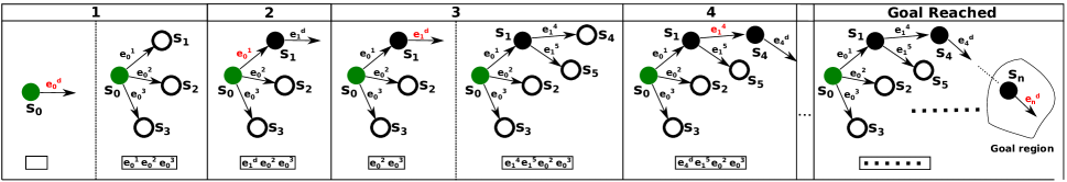
Figure 1: Example of eA*: (1) The dummy edge $e_{0}^{d}$ originating from $\mathbf{s}_{0}$ is expanded and the real edges $[e_{0}^{1},e_{0}^{2},e_{0}^{3}]$ are inserted into OPEN. (2) $e_{0}^{1}$ is expanded, during which it is evaluated and the successor $\mathbf{s}_{1}$ is generated. A dummy edge $e_{1}^{d}$ from $\mathbf{s}_{1}$ is inserted into OPEN. (3) $e_{1}^{d}$ is expanded and the real edges $[e_{1}^{4},e_{1}^{5}]$ are inserted into OPEN. (4) $e_{1}^{4}$ is expanded, during which it is evaluated and the successor $\mathbf{s}_{4}$ is generated and a dummy edge $e_{4}^{d}$ is inserted into open. This goes on until a dummy edge $e^{d}_{n}$ is expanded whose source state belongs to the goal region i.e. $\mathbf{s}_{n}\in\mathcal{G}$.

ePA*SE leverages the key algorithmic contribution of PA*SE i.e. parallel expansions of independent states but instead uses it to parallelize edge evaluations. In doing so, ePA*SE further improves the efficiency of PA*SE in domains with expensive to evaluate edges. ePA*SE obeys the same invariant as A* and PA*SE that when a state is expanded, its g-value is optimal. Therefore, every state is expanded at most once. However, unlike in PA*SE, where each thread is responsible for expanding a single state at a time, each ePA*SE thread is responsible for evaluating a single edge at a time. In order to build up to ePA*SE, we first describe a serial version of the proposed algorithm eA* (Edge-based A*). We then explain how eA* can be parallelized to get to ePA*SE, using the key idea behind PA*SE.

eA*

The first key algorithmic difference in eA* as compared to A* is that the open list OPEN contains edges instead of states. We introduce the term expansion of an edge and explicitly differentiate it from the expansion of a state. In A*, during the expansion of a state, all its successors are generated and, unless they have already been expanded, are either inserted into the open list or repositioned with the updated priority. In eA*, expansion of an edge $(\mathbf{s},\mathbf{a})$ involves evaluating the edge to generate the successor state $\mathbf{s}^{\prime}$ and adding/updating (but not evaluating) the edges originating from $\mathbf{s}^{\prime}$ into OPEN with the same priority of $g(\mathbf{s}^{\prime})+h(\mathbf{s}^{\prime})$. This choice of priority ensures that the edges originating from states that would have the same (state-) expansion priority in A* have the same (edge-) expansion priority in eA*. A state is defined as partially expanded if at least one (but not all) of its outgoing edges has been expanded or is under expansion, while it is defined as expanded if all its outgoing edges have been expanded. eA* uses the following data structures as the key ingredients of the algorithm.

• OPEN: A priority queue of edges (not states) that the search has generated but not expanded, where the edge with the smallest key/priority is placed in the front of the queue. The priority of an edge $e=(\mathbf{s},\mathbf{a})$ in OPEN is $f\left((\mathbf{s},\mathbf{a})\right)=g(\mathbf{s})+h(\mathbf{s})$.

• BE: The set of states that are partially expanded.

• CLOSED: The set of states that have been expanded.

Naively storing edges instead of states in OPEN introduces an inefficiency. In A*, the g-value of a state $\mathbf{s}$ can change many times during the search until the state is expanded at which point it is added to CLOSED. Every time this happens, OPEN has to be rebalanced to reposition $\mathbf{s}$. In eA*, every time $g(\mathbf{s})$ changes, the position of all of the outgoing edges from $\mathbf{s}$ need to be updated in OPEN. This increases the number of times OPEN has to be rebalanced, which is an expensive operation. However, since the edges originating from $\mathbf{s}$ have the same priority i.e. $g(\mathbf{s})+h(\mathbf{s})$, this can be avoided by replacing all the outgoing edges from $\mathbf{s}$ by a single dummy edge $e^{d}=(\mathbf{s},\mathbf{a^{d}})$, where $\mathbf{a^{d}}$ stands for a dummy action. The dummy edge stands as a placeholder for all the real edges originating from $\mathbf{s}$. Every time $g(\mathbf{s})$ changes, only the dummy edge has to be repositioned. Unlike what happens when a real edge is expanded, when the dummy edge $(\mathbf{s},\mathbf{a^{d}})$ is expanded, it is replaced by the outgoing real edges from $\mathbf{s}$ in OPEN. When a state’s dummy edge is expanded or is under expansion, it is also considered to be partially expanded and is therefore added to BE. When all the outgoing real edges of a state have been expanded, it is moved from BE to CLOSED. The g-value $g(\mathbf{s})$ of a state $\mathbf{s}$ in either BE or CLOSED can no longer change and hence the real edges originating from $\mathbf{s}$ will never have to be updated in OPEN.

eA* can be trivially extended to handle an inflation factor on the heuristic like wA* which leads to a more goal-directed search w-eA* (Weighted eA*). Fig. 1 show an example of w-eA* in action. Let $e_{i}^{j}$ refer to an edge from state $\mathbf{s}_{i}$ to $\mathbf{s}_{j}$ and $e^{d}_{i}$ refer to a dummy edge from $\mathbf{s}_{i}$. The states that are generated are shown in solid circles. The hollow circles represent states that are not generated and hence the incoming edges to these states are not evaluated. During the first expansion, the dummy edge $e^{d}_{0}$ originating from $\mathbf{s}_{0}$ is expanded and the real edges $[e_{0}^{1},e_{0}^{2},e_{0}^{3}]$ are inserted into OPEN. In the second expansion, the edge $e_{0}^{1}$ is expanded, during which it is evaluated and the successor $\mathbf{s}_{1}$ is generated. A dummy edge ($e^{d}_{1}$) from $\mathbf{s}_{1}$ is inserted into OPEN. In the third expansion, $e_{1}^{d}$ is expanded and the real edges $[e_{1}^{4},e_{1}^{5}]$ are inserted into OPEN. In the fourth expansion, the edge $e_{1}^{4}$ is expanded, during which it is evaluated and the successor $\mathbf{s}_{4}$ is generated and a dummy edge $e^{d}_{4}$ is inserted into open. This goes on until a dummy edge $e^{d}_{n}$ is expanded whose source state belongs to the goal region i.e. $\mathbf{s}_{n}\in\mathcal{G}$.

If the heuristic is informative, w-eA* evaluates fewer edges than wA*. In the example shown in Fig. 1, the edges $[e_{0}^{2},e_{0}^{3},e_{1}^{5}]$ do not get evaluated. Since wA* evaluates all outgoing edges of an expanded state, these edges would be evaluated in the case of wA* (with the same heuristic and inflation factor) when their source states are expanded ($\mathbf{s}_{0}$ and $\mathbf{s}_{1}$). Additionally, similar to how wPA*SE parallelizes wA*, w-eA* can be parallelized to obtain a highly efficient algorithm w-ePA*SE. Since w-ePA*SE is a trivial extension of ePA*SE, we instead describe how eA* can be parallelized to obtain ePA*SE.

eA* to ePA*SE

eA* can be parallelized using the key idea behind PA*SE i.e. parallel expansion of independent states, and applying it to edge expansions, resulting in ePA*SE. ePA*SE has two key differences from PA*SE that makes it more efficient:

1. Evaluation of edges is decoupled from the expansion of the source state giving the search the flexibility to figure out what edges need to be evaluated.

2. Evaluation of edges is parallelized.

In addition to OPEN and CLOSED, PA*SE uses another data structure BE (Being Expanded) to store the set of states currently being expanded by one of the threads. It uses a pairwise independence check on states in the open list to find states that are safe to expand in parallel. A state $\mathbf{s}$ is safe to expand if $g(\mathbf{s})$ is already optimal. In other words, there is no other state that is currently being expanded (in BE), nor in OPEN that can reduce $g(\mathbf{s})$. Formally, a state $\mathbf{s}$ is defined to be independent of state $\mathbf{s}$’ iff

$$g(\mathbf{s})-g(\mathbf{s}^{\prime})\leq h(\mathbf{s}^{\prime},\mathbf{s})$$ (1)

It can be proved that $\mathbf{s}$ is independent of states in OPEN that have a larger priority than $\mathbf{s}$ (Phillips, Likhachev, and Koenig 2014). However, the independence check has to be performed against the states in OPEN with a smaller priority than $\mathbf{s}$ as well as the states that are in BE.

Like in eA*, BE in ePA*SE stores the states that are partially expanded, as per the definition of partial expansion in eA*. Since ePA*SE stores edges in OPEN instead of states and each ePA*SE thread expands edges instead of states, the independence check has to be modified. An edge $e$ is safe to expand if Equations 2 and 3 hold.

$$\begin{split}g(e.\mathbf{s})-g(e^{\prime}.\mathbf{s})\leq h(e^{\prime}.\mathbf{s},e.\mathbf{s})\\ \forall e^{\prime}\in\textit{OPEN}~{}|~{}f\left(e^{\prime}\right)<f\left(e\right)\end{split}$$ (2)

$$\begin{split}g(e.\mathbf{s})-g(\mathbf{s}^{\prime})\leq h(\mathbf{s}^{\prime},e.\mathbf{s})~{}\forall\mathbf{s}^{\prime}\in\textit{BE}\end{split}$$ (3)

Equation 2 ensures that there is no edge in OPEN with a priority smaller than that of $e$, that upon expansion, can lower the g-value of $e.\mathbf{s}$ and hence lower the priority of $e$. In other words, the source state $\mathbf{s}$ of edge $e$ is independent of the source states of all edges in OPEN which have a smaller priority than $e$. Equation 3 ensures that there is no partially expanded state which can lower the g-value of $e.\mathbf{s}$. In other words, the source state $\mathbf{s}$ of edge $e$ is independent of all states in BE.

Details

Algorithm 1 ePA*SE

1:$\mathcal{A}\leftarrow\text{ action space }$, $N_{t}\leftarrow$ number of threads, $G\leftarrow\emptyset$

2:$\mathbf{s}_{0}\leftarrow\text{ start state }$, $\mathcal{G}\leftarrow\text{ goal region}$, $terminate\leftarrow\text{False}$

3:procedure Plan

4:     $\forall\mathbf{s}\in G$, $\mathbf{s}.g\leftarrow\infty$, $n\_successors\_generated(s)=0$

5:     $\mathbf{s}_{0}.g\leftarrow 0$

6:     insert $(\mathbf{s}_{0},\mathbf{a^{d}})$ in OPEN $\triangleright$ Dummy edge from $\mathbf{s}_{0}$

7:     LOCK

8:     while $\textbf{not }terminate$ do

9:         if $\textit{OPEN}=\emptyset\textbf{ and }\textit{BE}=\emptyset$ then

10:              $terminate=\text{True}$

11:              UNLOCK

12:              $\textbf{return}{}~{}\emptyset$          

13:         remove an edge $(\mathbf{s},\mathbf{a})$ from OPEN that has the
          smallest $f((\mathbf{s},\mathbf{a}))$ among all states in OPEN that
          satisfy Equations 2 and 3

14:         if such an edge does not exist then

15:              UNLOCK

16:              wait until OPEN or BE change

17:              LOCK

18:              continue          

19:         if $\mathbf{s}\in\mathcal{G}$ then

20:              $terminate=\text{True}$

21:              UNLOCK

22:              return Backtrack($\mathbf{s}$)

23:         else

24:              UNLOCK

25:              while $(\mathbf{s},\mathbf{a})$ has not been assigned a thread do

26:                  for $i=1:N_{t}$ do

27:                       if thread $i$ is available then

28:                           if thread $i$ has not been spawned then

29:                                Spawn $\textsc{EdgeExpandThread}(i)$                            

30:                           Assign $(\mathbf{s},\mathbf{a})$ to thread $i$                                                        

31:              LOCK               

32:     $terminate=\text{True}$

33:     UNLOCK

34:procedure EdgeExpandThread($i$)

35:     while $\textbf{not }terminate$ do

36:         if thread $i$ has been assigned an edge $(\mathbf{s},\mathbf{a})$ then

37:              $\textsc{Expand}\left((\mathbf{s},\mathbf{a})\right)$               

38:procedure Expand($(\mathbf{s},\mathbf{a})$)

39:     LOCK

40:     if $\mathbf{a}=\mathbf{a^{d}}$ then

41:         insert $\mathbf{s}$ in BE

42:         for $\mathbf{a}\in\mathcal{A}$ do

43:              $f\left((\mathbf{s},\mathbf{a})\right)=g(\mathbf{s})+h(\mathbf{s})$

44:              insert $(\mathbf{s},\mathbf{a})$ in OPEN with $f\left((\mathbf{s},\mathbf{a})\right)$          

45:     else

46:         UNLOCK

47:         $\mathbf{s}^{\prime},c\left((\mathbf{s},\mathbf{a})\right)\leftarrow\textsc{GenerateSuccessor}\left((\mathbf{s},\mathbf{a})\right)$

48:         LOCK

49:         if $\mathbf{s}^{\prime}\notin\textit{CLOSED}\cup\textit{BE}$ and

50:            $g(\mathbf{s}^{\prime})>g(\mathbf{s})+c\left((\mathbf{s},\mathbf{a})\right)$ then

51:              $g(\mathbf{s}^{\prime})=g(\mathbf{s})+c\left((\mathbf{s},\mathbf{a})\right)$

52:              $\mathbf{s}^{\prime}.parent=\mathbf{s}$

53:              $f\left((\mathbf{s}^{\prime},\mathbf{a^{d}})\right)=g(\mathbf{s}^{\prime})+h(\mathbf{s}^{\prime})$

54:              insert/update $(\mathbf{s}^{\prime},\mathbf{a^{d}})$ in OPEN with $f\left((\mathbf{s}^{\prime},\mathbf{a^{d}})\right)$          

55:         $n\_successors\_generated(\mathbf{s})+=1$

56:         if $n\_successors\_generated(\mathbf{s})=|\mathcal{A}|$ then

57:              remove $\mathbf{s}$ from BE

58:              insert $\mathbf{s}$ in CLOSED               

59:     UNLOCK

The pseudocode for ePA*SE is presented in Alg. 1. The main planning loop in Plan runs on a single thread (thread $0$), and in Line 13, an edge is removed for expansion from OPEN that has the smallest possible priority and is also safe to expand, as per Equations 2 and 3. If such an edge is not found, the thread waits for either OPEN or BE to change in Line 16. If a safe to expand edge is found, such that the source state of the edge belongs to the goal region, the solution path is returned by backtracking from the state to the start state using back pointers (like in A*) in Line 22. Otherwise, the edge is expanded assigned to an edge expansion thread (thread $i=1:N_{t}$) in Line 30. The edge expansion threads are spawned as and when needed to avoid the overhead of running unused threads (Line 29). The search terminates when either a solution is found, or when OPEN is empty and all threads are idle (BE is empty), in which case there is no solution.

If the edge to be expanded is a dummy edge, the source $\mathbf{s}$ of the edge is marked as partially expanded by adding it to BE (Line 41). The real edges originating from $\mathbf{s}$ are added to OPEN with the same priority as that of the dummy edge i.e. $g(\mathbf{s})+h(\mathbf{s})$. If the expanded edge is not a dummy edge, it is evaluated (Line 47) to obtain the successor $\mathbf{s}^{\prime}$ and the edge cost $c\left((\mathbf{s},\mathbf{a})\right)$. This is the expensive operation that ePA*SE seeks to parallelize, which is why it happens lock-free. If the expanded edge reduces $g(\mathbf{s}^{\prime})$, the dummy edge originating from $\mathbf{s}^{\prime}$ is added/updated in OPEN. A counter $n\_successors\_generated$ keeps track of the number of outgoing edges that have been expanded for every state. Once all the outgoing edges for a state have been expanded, and hence the state has been expanded, it is removed from BE and added to CLOSED (Lines 57 and 58).

Thread management

In PA*SE, the state expansion threads are spawned at the start and each of them independently pulls out states from the open list to expand. When the number of threads is higher than the number of independent states available for expansion at any point in time, the operating system has an unnecessary overhead of spinning unused threads. This causes the overall performance to go down as the number of unused threads goes up (see Fig. 6 in  (Phillips, Likhachev, and Koenig 2014)). Our initial experiments showed that using a similar thread management strategy in ePA*SE leads to a similar degradation in performance as the number of threads is increased beyond the optimal number of threads, even though the peak performance of ePA*SE is substantially higher than that of PA*SE. In order to prevent this degradation in performance, ePA*SE employs a different thread management strategy. There is a single thread that pulls out edges from the open list and it spawns edge expansion threads as needed but capped at $N_{t}$ (Line 29). When $N_{t}$ is higher than the number of independent edges available for expansion at any point in time, only a subset of available threads get spawned preventing performance degradation, as we will show in our experiments.

w-ePA*SE

w-ePA*SE is a bounded suboptimal variant of ePA*SE that trades off optimality for faster planning. Similar to wPA*SE, w-ePA*SE introduces two inflation factors, the first of which, $\epsilon\geq 1$, relaxes the independence rule (Equations 2 and 3) as follows.

$$\begin{split}g(e.\mathbf{s})-g(e^{\prime}.\mathbf{s})\leq\epsilon h(e^{\prime}.\mathbf{s},e.\mathbf{s})\\ \forall e^{\prime}\in\textit{OPEN}~{}|~{}f\left(e^{\prime}\right)<f\left(e\right)\end{split}$$ (4)

$$\begin{split}g(e.\mathbf{s})-g(\mathbf{s}^{\prime})\leq\epsilon h(\mathbf{s}^{\prime},e.\mathbf{s})~{}\forall\mathbf{s}^{\prime}\in\textit{BE}\end{split}$$ (5)

The second factor $w\geq 1$ is used to inflate the heuristic in the priority of edges in OPEN i.e. $f\left((\mathbf{s},\mathbf{a})\right)=g(\mathbf{s})~{}+~{}w~{}\cdot~{}h(\mathbf{s})$ which makes the search more goal directed. As long as $\epsilon\geq w$, the solution cost is bounded by $\epsilon\cdot c^{*}$ (Theorem 3). Note that $w$ can be greater than $\epsilon$, but then Equation 4 has to consider source states of all edges in OPEN and the solution cost will be bounded by $w\cdot c^{*}$ (Theorem 1). Since this leads to significantly more independence checks, the $\epsilon\geq w$ relationship is typically recommended in practice.

Properties

w-ePA*SE has identical properties to that of wPA*SE (Phillips, Likhachev, and Koenig 2014) and can be proved similarly with minor modifications.

Theorem 1 (Bounded suboptimal expansions)

When w-ePA*SE that performs independence checks against all states in BE and source states of all edges in OPEN, chooses an edge $e$ for expansion, then $g(e.\mathbf{s})\leq\lambda g^{*}(\mathbf{s})$, where $\lambda=\max(\epsilon,w)$.

Proof Assume, for the sake of contradiction, that $g(e.\mathbf{s})>\lambda g^{*}(e.\mathbf{s})$ directly before edge $e$ is expanded, and without loss of generality, that $g(e^{\prime}.\mathbf{s})\leq\lambda g^{*}(e^{\prime}.\mathbf{s})$ for all edges $e^{\prime}$ selected for expansion before $e$ (Assumption). Let $\mathbf{s}=e.\mathbf{s}$ for ease of notation. Consider any cost-minimal path $\pi(\mathbf{s}_{0},\mathbf{s})$ from $\mathbf{s}_{0}$ to $\mathbf{s}$. Let $\mathbf{s}_{m}$ be the closest state to $\mathbf{s}_{0}$ on $\pi(\mathbf{s}_{0},\mathbf{s})$ such that either 1) there exists at least one edge in OPEN with source state $\mathbf{s}_{m}$ or 2) $\mathbf{s}_{m}$ is in BE. $\mathbf{s}_{m}$ is no farther away from $\mathbf{s}_{0}$ on $\pi(\mathbf{s}_{0},\mathbf{s})$ than $\mathbf{s}$ since $e$ is in OPEN. Therefore, let $\pi(\mathbf{s}_{0},\mathbf{s}_{m})$ and $\pi(\mathbf{s}_{m},\mathbf{s})$ be the subpaths of $\pi(\mathbf{s}_{0},\mathbf{s})$ from $\mathbf{s}_{0}$ to $\mathbf{s}_{m}$ and from $\mathbf{s}_{m}$ to $\mathbf{s}$, respectively.

If $\mathbf{s}_{m}=\mathbf{s}_{0}$, then $g(\mathbf{s}_{m})\leq\lambda g^{*}(\mathbf{s}_{m})$ since $g(\mathbf{s}_{0})=g^{*}(\mathbf{s}_{0})=0$ ($\textbf{Contradiction}~{}\boldsymbol{1}$). Otherwise, let $\mathbf{s}_{p}$ be the predecessor of $\mathbf{s}_{m}$ on $\pi(\mathbf{s}_{0},\mathbf{s})$. $\mathbf{s}_{p}$ has been expanded (i.e. all edges outgoing edges of $\mathbf{s}_{p}$ have been expanded) since every state closer to $\mathbf{s}_{0}$ on $\pi(\mathbf{s}_{0},\mathbf{s})$ than $\mathbf{s}_{m}$ has been expanded (since every unexpanded state on $\pi(\mathbf{s}_{0},\mathbf{s})$ different from $\mathbf{s}_{0}$ is either in BE or has an outgoing edge in OPEN, or has a state closer to $\mathbf{s}_{0}$ on $\pi(\mathbf{s}_{0},\mathbf{s})$ that is either in BE or has an outgoing edge in OPEN). Therefore, since all outgoing edges from $\mathbf{s}_{p}$ have been expanded, $g(\mathbf{s}_{p})\leq\lambda g^{*}(\mathbf{s}_{p})$ because of Assumption. Then, because of the $g$ update of $\mathbf{s}_{m}$ when the edge from $\mathbf{s}_{p}$ to $\mathbf{s}_{m}$ was expanded,

$$g(\mathbf{s}_{m}) \leq g(\mathbf{s}_{p})+c(\mathbf{s}_{p},\mathbf{s}_{m})$$

$$\leq\lambda g^{*}(\mathbf{s}_{p})+c(\mathbf{s}_{p},\mathbf{s}_{m})$$ (6)

Since $\mathbf{s}_{p}$ is the predecessor of $\mathbf{s}_{m}$ on the cost-minimal path $\pi(\mathbf{s}_{0},\mathbf{s})$,

$$g^{*}(\mathbf{s}_{m})=g^{*}(\mathbf{s}_{p})+c(\mathbf{s}_{p},\mathbf{s}_{m})$$

$$\implies g^{*}(\mathbf{s}_{p})=g^{*}(\mathbf{s}_{m})-c(\mathbf{s}_{p},\mathbf{s}_{m})$$ (7)

Substituting $g^{*}(\mathbf{s}_{p})$ from Equation Properties into Equation Properties,

$$\implies g(\mathbf{s}_{m})\leq\lambda g^{*}(\mathbf{s}_{m})-(\lambda-1)c(\mathbf{s}_{p},\mathbf{s}_{m})$$

$$\implies g(\mathbf{s}_{m})\leq\lambda g^{*}(\mathbf{s}_{m})$$

$$\implies \lambda c(\pi(\mathbf{s}_{0},\mathbf{s}_{m}))=\lambda g^{*}(\mathbf{s}_{m})\geq g(\mathbf{s}_{m})$$ (8)

Since $h(\mathbf{s}_{m},\mathbf{s})$ satisfies forward-backward consistency and is therefore admissible, $h(\mathbf{s}_{m},\mathbf{s})\leq c(\pi(\mathbf{s}_{m},\mathbf{s}))$. Since, $\lambda=\max(\epsilon,w)$, $\epsilon\leq\lambda$,

$$\lambda c(\pi(\mathbf{s}_{m},\mathbf{s}))\geq\lambda h(\mathbf{s}_{m},\mathbf{s})\geq\epsilon h(\mathbf{s}_{m},\mathbf{s})$$ (9)

Adding Properties and 9,

$$\lambda c(\mathbf{s}_{0},\mathbf{s}) =\lambda c(\mathbf{s}_{0},\mathbf{s}_{m})+\lambda c(\mathbf{s}_{m},\mathbf{s})$$

$$\geq g(\mathbf{s}_{m})+\epsilon h(\mathbf{s}_{m},\mathbf{s})$$ (10)

Assuming w-ePA*SE performs independence checks against states in BE and source states of all edges in OPEN when choosing an edge $e$ with source $e.\mathbf{s}$ to expand, and $\mathbf{s}_{m}$ is either in BE or there exists atleast one edge with source $\mathbf{s}_{m}$ in OPEN,

$$\epsilon h(e^{\prime}.\mathbf{s},e.\mathbf{s})\geq g(e.\mathbf{s})-g(e^{\prime}.\mathbf{s})$$

$$\forall e^{\prime}\in\textit{OPEN}~{}|~{}e^{\prime}.\mathbf{s}=\mathbf{s}_{m}$$

$$\implies g(\mathbf{s}_{m})+\epsilon h(\mathbf{s}_{m},\mathbf{s})\geq g(\mathbf{s})$$ (11)

Therefore,

$$\lambda g^{*}(\mathbf{s})= \lambda c(\pi(\mathbf{s}_{0},\mathbf{s}))$$

$$\geq g(\mathbf{s}_{m})+\epsilon h(\mathbf{s}_{m},\mathbf{s})$$ (Using Eq. Properties)

$$\geq g(\mathbf{s})$$ (Using Eq. Properties)

($$\textbf{Contradiction}~{}\boldsymbol{2}$$)

Contradiction 1 and Contradiction 2 invalidate the Assumption, which proves Theorem 1.

Theorem 2

If $w\leq\epsilon$, and considering any two edges $e$ and $e$’ in OPEN, the source state of $e$ is independent of the source state of $e$’ if $f(e)\leq f(e^{\prime})$.

Proof

$$f(e) \leq f(e^{\prime})$$

$$\implies g(e.\mathbf{s})+wh(e.\mathbf{s}) \leq g(e^{\prime}.\mathbf{s})+wh(e^{\prime}.\mathbf{s})$$

$$\implies g(e.\mathbf{s}) \leq g(e^{\prime}.\mathbf{s})+w(h(e^{\prime}.\mathbf{s})-h(e.\mathbf{s}))$$

$$\leq g(e^{\prime}.\mathbf{s})+wh(e^{\prime}.\mathbf{s},e.\mathbf{s})$$

(forward-backward consistency)

$$\leq g(e^{\prime}.\mathbf{s})+\epsilon h(e^{\prime}.\mathbf{s},e.\mathbf{s})$$

(since $$w\leq\epsilon$$)

Therefore, $e.\mathbf{s}$ is independent of $e^{\prime}.\mathbf{s}$ by definition (Eq. 1).

Theorem 3 (Bounded suboptimality)

If $w\leq\epsilon$, and w-ePA*SE chooses a dummy edge $e^{d}=(\mathbf{s},\mathbf{a^{d}})$ for expansion, such that the source state $\mathbf{s}$ belongs to the goal region i.e. $\mathbf{s}\in\mathcal{G}$, then $g(\mathbf{s})\leq\epsilon g^{*}(\mathbf{s})=\epsilon\cdot c^{*}$.

Proof This directly follows from Theorems 1 and 2.

Theorem 4 (Completeness)

If there exists at least one path $\pi$ in $G$ from $\mathbf{s}_{0}$ to $\mathcal{G}$, w-ePA*SE will find it.

Proof This proof makes use of Theorem 3 and is similar to the equivalent proof of serial wA*.

Evaluation

We evaluate w-ePA*SE in two planning domains where edge evaluation is expensive. All experiments were carried out on Amazon Web Services (AWS) instances. All algorithms were implemented in C++.

3D Navigation

The first domain is motion planning for 3D ($x,y,\theta$) navigation of a PR2, which is a human-scale dual-arm mobile manipulator robot, in an indoor environment similar to the one used in (Narayanan and Likhachev 2017) and shown in Fig. 2. Here $x,y$ are the planar coordinates and $\theta$ is the orientation of the robot. The robot can move along 18 simple motion primitives that independently change the three state coordinates by incremental amounts. Evaluating each primitive involves collision checking of the robot model (approximated as spheres) against the world model (represented as a 3D voxel grid) at interpolated states on the primitive. Though approximating the robot with spheres instead of meshes speeds up collision checking, it is still the most expensive component of the search. The computational cost of edge evaluation increases with an increasing granularity of interpolated states at which collision checking is carried out. For our experiments, collision checking is carried out at interpolated states $1$ $\mathrm{cm}$ apart. The search uses Euclidean distance as the admissible heuristic. We evaluate on 50 trials in each of which the start configuration of the robot and goal region are sampled randomly. We compare w-ePA*SE with other CPU-based parallel search baselines. The first baseline is a variant of weighted A* in which during a state expansion, the successors of the state are generated and the corresponding edges are evaluated in parallel. For lack of a better term, we call this baseline Parallel Weighted A* (PwA*). Note that this is very different from the Parallel A* (PA*) algorithm (Irani and Shih 1986) which has already been shown to underperform wPA*SE (Phillips, Likhachev, and Koenig 2014). The second baseline is wPA*SE. These two baselines leverage parallelization differently. PwA* parallelizes the generation of successors, whereas wPA*SE parallelizes state expansions. w-ePA*SE on the other hand parallelizes edge evaluations. We also compare against a variation of w-ePA*SE (w-ePA*SE w/o thread mgt.) that uses the thread management strategy of wPA*SE as opposed to the improved thread management strategy described in the Method. Speedup over wA* is defined as the ratio of the average runtime of wA* over the average runtime of a specific algorithm.

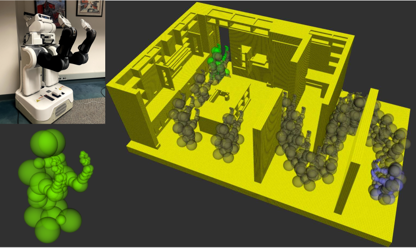
Figure 2: (Navigation) Left: The PR2’s collision model is approximated with spheres. Right: The task is to navigate in an indoor map from a given start (purple) and goal (green) states using a set of motion primitives. States at the end of every primitive in the generated plan are shown in black.

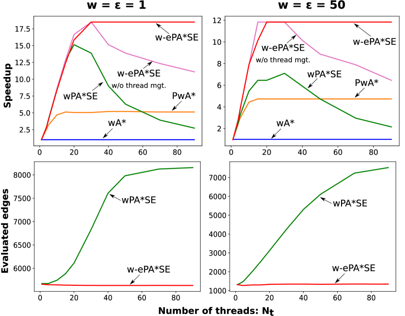
Figure 3: (Navigation) Top: Average speedup achieved by PwA*, wPA*SE and w-ePA*SE over wA*. Bottom: Number of edges evaluated by wPA*SE and w-ePA*SE.

$N_{t}$	1	4	5	10	15	20	30	40	50	70	90
wA*	3.33	-	-	-	-	-	-	-	-	-	-	$w=\epsilon=1\ \$
PwA*	3.37	1.31	1.06	0.71	0.65	0.66	0.66	0.64	0.64	0.65	0.65
wPA*SE	3.37	1.14	0.85	0.39	0.26	0.22	0.24	0.37	0.53	0.85	1.22
w-ePA*SE w/o thread mgt.	3.43	1.17	0.88	0.39	0.26	0.20	0.18	0.22	0.24	0.27	0.30
w-ePA*SE	3.34	1.17	0.87	0.40	0.27	0.21	0.18	0.18	0.18	0.18	0.18

wA*	0.71	-	-	-	-	-	-	-	-	-	-	$w=\epsilon=50$
PwA*	0.72	0.29	0.24	0.16	0.15	0.15	0.15	0.15	0.15	0.15	0.15
wPA*SE	0.71	0.28	0.22	0.13	0.11	0.11	0.10	0.12	0.15	0.24	0.33
w-ePA*SE w/o thread mgt.	0.75	0.25	0.19	0.09	0.06	0.06	0.06	0.07	0.08	0.09	0.11
w-ePA*SE	0.72	0.25	0.19	0.09	0.07	0.06	0.06	0.06	0.06	0.06	0.06

Table 1: (Navigation) Average planning times ($\mathrm{s}$) for wA*, PwA*, wPA*SE and w-ePA*SE for varying $N_{t}$, with $w=\epsilon=1$ (top) and with $w=\epsilon=50$ (bottom).

$N_{t}$	1	4	5	10	15	20	30	40	50	70	90
wPA*SE	5674	5673	5676	5746	5885	6112	6826	7607	7980	8125	8156	$w=\epsilon=1\ \$
w-ePA*SE	5660	5650	5649	5645	5640	5637	5634	5633	5633	5634	5633

wPA*SE	1309	1451	1526	2028	2561	3121	4251	5307	6105	7231	7526	$w=\epsilon=50$
w-ePA*SE	1324	1273	1277	1300	1301	1333	1343	1345	1334	1348	1343

Table 2: (Navigation) Number of edges evaluated by wPA*SE and w-ePA*SE for varying $N_{t}$, with $w=\epsilon=1$ (top) and with $w=\epsilon=50$ (bottom).

Fig. 3 (top) shows the average speedup achieved by wPA*SE and the baselines over wA* for varying $N_{t}$, for $w=\epsilon=1$ and $w=\epsilon=50$. The corresponding raw planning times are shown in Table 1. The speedup achieved by PwA* saturates at the branching factor of the domain. This is expected since PwA* parallelizes the evaluation of the outgoing edges of a state being expanded. If $N_{t}$ is greater than the branching factor $M$, $N_{t}-M$ threads remain unutilized. For low $N_{t}$, the speedup achieved by w-ePA*SE matches that of wPA*SE. However, for high $N_{t}$, the speedup achieved by w-ePA*SE rapidly outpaces that of w-ePA*SE, especially for the inflated heuristic case. This is because w-ePA*SE is much more efficient than wPA*SE since it parallelizes edge evaluations instead of state expansions. This increased efficiency is more apparent with the availability of a larger computational budget in the form of a greater number of threads to allocate to evaluating edges. The speedup of wPA*SE reaches a peak and then rapidly deteriorates. This is also the case for w-ePA*SE w/o (improved) thread mgt. (described in the Method), even though the peak speedup of w-ePA*SE w/o thread mgt.is higher than that of wPA*SE. However, the speedup of w-ePA*SE with the improved thread management strategy reaches a maximum and then saturates instead of degrading. This is due to the difference in the multithreading strategy employed by w-ePA*SE as explained in the Method.

Fig. 3 (bottom) and Table 2 show that w-ePA*SE evaluates significantly fewer edges as compared to wPA*SE. With a greater number of threads, the difference is significant. This indicates that beyond parallelization of edge evaluations, the w-eA* formulation that w-ePA*SE uses has another advantage that if the heuristic is informative, w-ePA*SE evaluates fewer edges than wPA*SE, which contributes to the lower planning time of w-ePA*SE. The intuition behind this is that in wA*, the evaluation of the outgoing edges from a given state is tightly coupled with the expansion of the state because all the outgoing edges from a given state must be evaluated at the same time when the state is expanded. In w-eA* the evaluation of these edges is decoupled from each other since the search expands edges instead of states.

Assembly Task

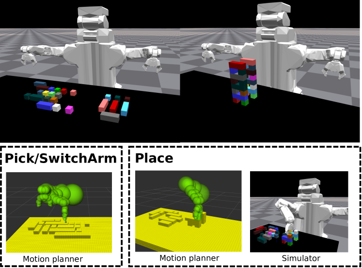
Figure 4: (Assembly) Top: The PR2 has to arrange a set of blocks on the table (left) into a given configuration (right). Bottom: It is equipped with Pick, Place and SwitchArm controllers. The Pick controller uses the motion planner to reach a block. The Place controller uses the motion planner to place a block and simulates the outcome of releasing the block. The SwitchArm controller uses the motion planner to move the active arm to a home position.

	wA*	PwA*	wPA*SE	w-ePA*SE
$N_{t}$	1	25	10	10
Time (s)	3010	1066	419	301
Speedup	1	2.8	7.2	10

Table 3: (Assembly) Average planning times and speedup over wA* for w-ePA*SE and the baselines.

The second domain is a task and motion planning problem of assembling a set of blocks on a table into a given structure by a PR2, as shown in Fig. 4. This domain is similar to the one introduced in (Mukherjee, Aine, and Likhachev 2022), but in this work, we enable the dual-arm functionality of the PR2. We assume full state observability of the 6D poses of the blocks and the robot’s joint configuration. The goal is defined by the 6D poses of each block in the desired structure. The PR2 is equipped with Pick and Place controllers which are used as macro-actions in the high-level planning. In addition, there is a SwitchArm controller which switches the active arm by moving the current active arm to a home position. All of these actions use a motion planner internally to compute collision-free trajectories in the workspace. Additionally, Place has access to a simulator (NVIDIA Isaac Gym (Makoviychuk et al. 2021)) to simulate the outcome of placing a block at its desired pose. For example, if the planner tries to place a block at its final pose but has not placed the block underneath yet, the placed block will not be supported and the structure will not be stable. This would lead to an invalid successor during planning. We set a simulation timeout of $t_{s}=0.2$ $\mathrm{s}$ to evaluate the outcome of placing a block. Considering the variability in the simulation speed and the overhead of communicating with the simulator, this results in a total wall time of less than $2$ $\mathrm{s}$ for the simulation. The motion planner has a timeout of $t_{p}=60$ $\mathrm{s}$ based on the wall time, and therefore that is the maximum time the motion planning can take. Successful Pick, Place and SwitchArm actions have unit costs, and infinite otherwise. A Pick action on a block is successful if the motion planner finds a feasible trajectory to reach the block within $t_{p}$. A Place action on a block is successful if the motion planner finds a feasible trajectory to place the block within $t_{p}$ and simulating the block placement results in the block coming to rest at the desired pose within $t_{s}$. A SwitchArm action is successful if the motion planner finds a feasible trajectory to the home position for the active arm within $t_{p}$. The number of blocks that are not in their final desired pose is used as the admissible heuristic, with $w=\epsilon=5$. Table 3 shows planning times and speedup over wA* for w-ePA*SE and those of the baselines. We use 25 threads in the case of PwA* because that is the maximum branching factor in this domain. The numbers are averaged across 20 trials in each of which the blocks are arranged in random order on the table. Table 3 shows the average planning times and speedup over wA* of w-ePA*SE as compared to those of the lazy search baselines. w-ePA*SE achieves a 10x speedup over wA* and outperforms the baselines in this domain as well.

Conclusion and Future Work

We presented an optimal parallel search algorithm ePA*SE, that improves on PA*SE by parallelizing edge evaluations instead of state expansions. We also presented a sub-optimal variant w-ePA*SE and proved that it maintains bounded suboptimality guarantees. Our experiments showed that w-ePA*SE achieves an impressive reduction in planning time across two very different planning domains, which shows the generalizability of our conclusions. Empirically, we have observed w-ePA*SE to be a strict improvement over wPA*SE for domains with expensive to compute edges. Even though we also test with a relatively large budget of threads, the performance improvement is significant even with a smaller budget of fewer than 10 threads, which is the case with typical mobile computers. Therefore in practice, we recommend using w-ePA*SE in a planning domain where 1) the computational bottleneck is edge evaluations and 2) successor states cannot be generated without evaluating edges and therefore parallelized lazy planning i.e. MPLP (Mukherjee, Aine, and Likhachev 2022) is not applicable.

MPLP (Mukherjee, Aine, and Likhachev 2022) and ePA*SE use fundamentally different parallelization strategies. MPLP searches the graph lazily while evaluating edges in parallel, but relies on the assumption that states can be generated lazily without evaluating edges. On the other hand, ePA*SE evaluates edges in a way that preserves optimality without the need for state (and edge) re-expansions but does not rely on lazy state generation. In domains where states can be generated lazily, however, the lazy state generation takes a non-trivial amount of time, these two different parallelization strategies can be combined. Both MPLP and ePA*SE achieve a speedup at a certain number of threads, beyond which the speedup saturates. Therefore, utilizing both of them together will allow us to leverage more threads, which either of them on their own cannot.

References

- Aine et al. (2016) Aine, S.; Swaminathan, S.; Narayanan, V.; Hwang, V.; and Likhachev, M. 2016. Multi-heuristic A*. The International Journal of Robotics Research, 35(1-3): 224–243.
- Amato and Dale (1999) Amato, N. M.; and Dale, L. K. 1999. Probabilistic roadmap methods are embarrassingly parallel. In Proceedings 1999 IEEE International Conference on Robotics and Automation, volume 1, 688–694.
- Burns et al. (2010) Burns, E.; Lemons, S.; Ruml, W.; and Zhou, R. 2010. Best-first heuristic search for multicore machines. Journal of Artificial Intelligence Research, 39: 689–743.
- Butzke et al. (2014) Butzke, J.; Sapkota, K.; Prasad, K.; MacAllister, B.; and Likhachev, M. 2014. State lattice with controllers: Augmenting lattice-based path planning with controller-based motion primitives. In 2014 IEEE/RSJ International Conference on Intelligent Robots and Systems, 258–265.
- Devaurs, Siméon, and Cortés (2011) Devaurs, D.; Siméon, T.; and Cortés, J. 2011. Parallelizing RRT on distributed-memory architectures. In 2011 IEEE International Conference on Robotics and Automation, 2261–2266.
- Evett et al. (1995) Evett, M.; Hendler, J.; Mahanti, A.; and Nau, D. 1995. PRA*: Massively parallel heuristic search. Journal of Parallel and Distributed Computing, 25(2): 133–143.
- Hart, Nilsson, and Raphael (1968) Hart, P. E.; Nilsson, N. J.; and Raphael, B. 1968. A formal basis for the heuristic determination of minimum cost paths. IEEE transactions on Systems Science and Cybernetics, 4(2): 100–107.
- He et al. (2021) He, X.; Yao, Y.; Chen, Z.; Sun, J.; and Chen, H. 2021. Efficient parallel A* search on multi-GPU system. Future Generation Computer Systems, 123: 35–47.
- Ichnowski and Alterovitz (2012) Ichnowski, J.; and Alterovitz, R. 2012. Parallel sampling-based motion planning with superlinear speedup. In IROS, 1206–1212.
- Irani and Shih (1986) Irani, K.; and Shih, Y.-f. 1986. Parallel A* and AO* algorithms- An optimality criterion and performance evaluation. In 1986 International Conference on Parallel Processing, University Park, PA, 274–277.
- Jacobs et al. (2012) Jacobs, S. A.; Manavi, K.; Burgos, J.; Denny, J.; Thomas, S.; and Amato, N. M. 2012. A scalable method for parallelizing sampling-based motion planning algorithms. In 2012 IEEE International Conference on Robotics and Automation, 2529–2536.
- Jacobs et al. (2013) Jacobs, S. A.; Stradford, N.; Rodriguez, C.; Thomas, S.; and Amato, N. M. 2013. A scalable distributed RRT for motion planning. In 2013 IEEE International Conference on Robotics and Automation, 5088–5095.
- Kusnur et al. (2021) Kusnur, T.; Mukherjee, S.; Saxena, D. M.; Fukami, T.; Koyama, T.; Salzman, O.; and Likhachev, M. 2021. A planning framework for persistent, multi-uav coverage with global deconfliction. In Field and Service Robotics, 459–474. Springer.
- Liang et al. (2021) Liang, J.; Sharma, M.; LaGrassa, A.; Vats, S.; Saxena, S.; and Kroemer, O. 2021. Search-Based Task Planning with Learned Skill Effect Models for Lifelong Robotic Manipulation. arXiv preprint arXiv:2109.08771.
- Makoviychuk et al. (2021) Makoviychuk, V.; Wawrzyniak, L.; Guo, Y.; Lu, M.; Storey, K.; Macklin, M.; Hoeller, D.; Rudin, N.; Allshire, A.; Handa, A.; et al. 2021. Isaac Gym: High Performance GPU-Based Physics Simulation For Robot Learning. arXiv preprint arXiv:2108.10470.
- Mukherjee, Aine, and Likhachev (2022) Mukherjee, S.; Aine, S.; and Likhachev, M. 2022. MPLP: Massively Parallelized Lazy Planning. IEEE Robotics and Automation Letters, 7(3): 6067–6074.
- Mukherjee et al. (2021) Mukherjee, S.; Paxton, C.; Mousavian, A.; Fishman, A.; Likhachev, M.; and Fox, D. 2021. Reactive long horizon task execution via visual skill and precondition models. In 2021 IEEE/RSJ International Conference on Intelligent Robots and Systems (IROS), 5717–5724. IEEE.
- Narayanan and Likhachev (2017) Narayanan, V.; and Likhachev, M. 2017. Heuristic search on graphs with existence priors for expensive-to-evaluate edges. In Twenty-Seventh International Conference on Automated Planning and Scheduling.
- Park, Pan, and Manocha (2016) Park, C.; Pan, J.; and Manocha, D. 2016. Parallel motion planning using poisson-disk sampling. IEEE Transactions on Robotics, 33(2): 359–371.
- Phillips, Likhachev, and Koenig (2014) Phillips, M.; Likhachev, M.; and Koenig, S. 2014. PA* SE: Parallel A* for slow expansions. In Twenty-Fourth International Conference on Automated Planning and Scheduling.
- Pohl (1970) Pohl, I. 1970. Heuristic search viewed as path finding in a graph. Artificial intelligence, 1(3-4): 193–204.
- Russell (2010) Russell, S. J. 2010. Artificial intelligence a modern approach. Pearson Education, Inc.
- Zhou and Zeng (2015) Zhou, Y.; and Zeng, J. 2015. Massively parallel A* search on a GPU. In Proceedings of the AAAI Conference on Artificial Intelligence.