Resonances near spectral thresholds for multichannel discrete Schrödinger operators

Abstract.

We study the distribution of resonances for discrete Hamiltonians of the form $H_{0}+V$ near the thresholds of the spectrum of $H_{0}$. Here, the unperturbed operator $H_{0}$ is a multichannel Laplace type operator on $\ell^{2}(\mathbb{Z};\mathfrak{G})\cong\ell^{2}(\mathbb{Z})\otimes\mathfrak{G}$ where ${\mathfrak{G}}$ is an abstract separable Hilbert space, and $V$ is a suitable non-selfadjoint compact perturbation. We distinguish two cases. If ${\mathfrak{G}}$ is of finite dimension, we prove that resonances exist and do not accumulate at the thresholds in the spectrum of $H_{0}$. Furthermore, we compute exactly their number and give a precise description on their location in clusters in the complex plane. If ${\mathfrak{G}}$ is of infinite dimension, an accumulation phenomenon occurs at some thresholds. We describe it by means of an asymptotical analysis of the counting function of resonances. Consequences on the distribution of the complex and the embedded eigenvalues are also given.

Mathematics subject classification 2020: 47A10, 81Q10, 81U24.

1. Introduction

1.1. General setting

Let $\Delta$ be the positive one-dimensional discrete Laplacian defined on the Hilbert space

$\ell^{2}(\mathbb{Z}):=\big{\{}u:\mathbb{Z}\to\mathbb{C};\,\|u\|^{2}=\sum_{n\in\mathbb{Z}}|u(n)|^{2}<\infty\big{\}},$

by

$$(\Delta u)(n):=2u(n)-u(n+1)-u(n-1),\;\;\;u\in\ell^{2}(\mathbb{Z}).$$

Consider a complex separable Hilbert space $\mathfrak{G}$ and let $M$ be a compact operator on $\mathfrak{G}$. On the Hilbert space $\ell^{2}(\mathbb{Z};\mathfrak{G})\cong\ell^{2}(\mathbb{Z})\otimes\mathfrak{G}$, we introduce the operator $H_{0}$ defined by

(1.1) $$H_{0}:=\Delta\otimes I_{\mathfrak{G}}+I_{\ell^{2}(\mathbb{Z})}\otimes M,$$

where $I_{\mathfrak{G}}$ and $I_{\ell^{2}(\mathbb{Z})}$ denote the identity operators on $\mathfrak{G}$ and $\ell^{2}(\mathbb{Z})$ respectively.

The operator $\Delta$ is bounded, selfadjoint in $\ell^{2}(\mathbb{Z})$ and its spectrum is absolutely continuous given by $\sigma(\Delta)=\sigma_{{\rm ac}}(\Delta)=[0,4]$. Then, the spectrum of $H_{0}$ is absolutely continuous (in particular there are not embedded eigenvalues) and it has the following band structure in the complex plane

$$\sigma(H_{0})=\sigma_{ac}(H_{0})=\bigcup_{\lambda\in\sigma(M)}[\lambda,\lambda+4],$$

where the edge points {$\lambda,\lambda+4\}_{\lambda\in\sigma(M)}$ play the role of thresholds. These bands are parallel to the real axis, and may be pairwise disjoint, overlapping or intersecting (see Fig. 1).

Figure 1. Schematic example of $\sigma(H_{0})$. ($\tau_{j}=\lambda_{j}+4$).

Our main purpose in this paper is to study the existence and the distribution of resonances for operators of the form $H=H_{0}+V$ near the spectral thresholds of $\sigma(H_{0})$. The specific class of perturbations $V:\ell^{2}(\mathbb{Z};\mathfrak{G})\to\ell^{2}(\mathbb{Z};\mathfrak{G})$ to be considered will be introduced later. The resonances will be defined as the poles of the meromorphic extension of the resolvent of $H$ in some weighted spaces (see Section 2).

We will study two different cases: the first one is when $\mathfrak{G}$ is finite-dimensional, and the second one is when $\mathfrak{G}$ is infinite-dimensional with $M$ a finite-rank operator on $\mathfrak{G}$. Although both cases may look similar, they present an important difference in terms of the distribution of resonances. In fact, since in the first case the spectrum of $M$ consists only on eigenvalues with finite multiplicities, and in the second one, $0$ is an eigenvalue of $M$ with infinite multiplicity, the set of spectral thresholds splits into two classes.

• The first class consists on the thresholds $\{\lambda,\lambda+4\}_{\lambda\in\sigma(M)}$ such that $\lambda$ is an eigenvalue of $M$ with finite multiplicity. Near such points, we prove the existence of resonances of $H$ and precise their location. More specifically, under suitable assumptions, we obtain the exact number of resonances near the thresholds, and we prove that they are distributed in clusters around some specific points, see Theorems 3.1 and 3.2 (this improves some of the results in [9]).

• The second class consists of the set of thresholds $\{0,4\}$ in the infinite dimensional case. In contrast to the first class, we show that there is an infinite number of resonances that accumulate near these points, see Theorem 3.4.

1.2. Comments on the literature

The resonance phenomena in quantum mechanics has been mathematically tackled from various perspectives. For instance, resonances of a stationary quantum system can be defined as the poles of a suitable meromorphic extension of either the Green function, the resolvent of the Hamiltonian or the scattering matrix. The imaginary part of such poles is sometimes interpreted as the inverse of the lifetime of some associated quasi-eigenstate. A related idea is to identify the resonances of a quantum Hamiltonian with the discrete eigenvalues of some non-selfadjoint operator obtained from the original one by the methods of spectral deformations. Another point of view consists in defining the resonances dynamically, i.e., in terms of quasi-exponential decay for the time evolution of the system. This property is somewhat encoded in the concept of sojourn time. The equivalence between these different perspectives and formalisms is also an issue.

The study of the existence and the asymptotic behavior of resonances in different asymptotic regimes has witnessed a lot of progress during the last thirty years, mainly in the context of continuous configuration spaces. This has been achieved thanks to the development of many mathematical approaches such as scattering methods, spectral and variational techniques, semiclassical and microlocal analysis (many references to this vast literature can be found in the monographs [17, 18, 11]).

On the other side, the qualitative spectral properties of the discrete Laplace operator and some selfadjoint generalizations exhibiting dispersive properties, have been extensively investigated. We primarily refer to [10, 30] for the multidimensional lattice case ${\mathbb{Z}}^{d}$, [12] and references therein for trees, [2, 26] for periodic graphs and perturbed graphs, respectively. Analyses of the continuum limit are performed in [24] and references therein. The role of the thresholds of the discrete Laplace operator are specifically studied in [19] (see also references therein). We also refer the reader to [28] and references therein for studies concerning Jacobi matrices and block Jacobi matrices.

The study of resonances for quantum Hamiltonians on discrete structures has been mainly performed on quasi 1D models (see [21] and references therein). However, in these approaches, perturbations are assumed to be diagonal and essentially compactly supported. One may quote [7] where results on the distribution of resonances of compact perturbations of the 1D discrete Laplace operator were obtained. This suggests that a more systematic analysis of resonances in the spirit of the works of Bony, Bruneau and Raikov [6, 5] should be performed in this context. The present paper is the first of a sequence of studies about resonances for operators on various graph structures where the perturbation is not necessarily diagonal. In what follows, we focus on some generalizations of the 1D discrete Laplace operator and study the distribution of resonances that appear in the neighborhoods of the thresholds, in perturbative regimes.

The asymptotic behavior of resonances near thresholds has been studied in an abstract setting in [15]. However, this study does not include the models of the present work. On the other side, in some continuous waveguides models, the singularities at the thresholds are similar in structure to the ones that appear in our case. Thus, related results to ours are obtained in [9, 8]. Nevertheless, using a modified approach, the conclusions that we obtain here are sharper. More precisely, as we said before, we provide the exact number of resonances near each threshold and we show that they are distributed in small clusters whose radii depend on the perturbation parameter. Moreover, we treat also a case of accumulation of resonances, which do not appear in the above works.

1.3. Plan of the article and notations:

The article is organized as follows: the resonances are defined in Section 2. The main results, namely Theorems 3.1, 3.2 and 3.4, are stated in Section 3. In Section 4 we briefly describe some models where our results can be applied. The proofs of the main theorems are postponed to Sections 5-8. Finally, in the appendix we prove a result on the multiplicity of resonances needed in our study. We present this result in an abstract form since it may be of independent interest.

Notations. Let $\mathcal{K}$ be a separable Hilbert space. We denote by $\mathcal{B}(\mathcal{K})$ the algebra of bounded linear operators acting on $\mathcal{K}$. $\mathfrak{S}_{\infty}(\mathcal{K})$ and $\mathfrak{S}_{p}(\mathcal{K})$, $p\geq 1$, stand for the ideal of compact operators and the Schatten classes respectively. In particular, $\mathfrak{S}_{1}(\mathcal{K})$ and $\mathfrak{S}_{2}(\mathcal{K})$ are the ideals of trace class operators and Hilbert-Schmidt operators on $\mathcal{K}$, endowed with the norms $\|\cdot\|_{1}$ and $\|\cdot\|_{2}$ respectively. If $U\subset\mathbb{C}$ is an open set, we denote $\text{Hol}(U;\mathcal{K})$ the set of holomorphic functions on $U$ with values in $\mathcal{K}$. We denote by $(\delta_{n})_{n\in\mathbb{Z}}$ the canonical basis of $\ell^{2}(\mathbb{Z})$. Throughout the paper, $\mathcal{H}$ stands for the Hilbert space $\ell^{2}(\mathbb{Z})\otimes\mathfrak{G}$ identified with $\ell^{2}(\mathbb{Z};\mathfrak{G})$, $(\delta_{n})_{n\in\mathbb{Z}}$ the canonical orthonormal basis of $\ell^{2}({\mathbb{Z}})$, and $(e_{j})_{j\in I}$ stands for an orthonormal basis of $\mathfrak{G}$, for some index set $I\subseteq\mathbb{Z}_{+}$. For $s>0$, let $W_{s}$ be the multiplication operator by the function $\mathbb{Z}\ni n\mapsto\|e^{-\frac{s}{2}|\cdot|}\|_{\ell^{2}(\mathbb{Z})}e^{\frac{s}{2}|n|}$ acting on $e^{-\frac{s}{2}|\cdot|}\ell^{2}(\mathbb{Z})$ with values in $\ell^{2}(\mathbb{Z})$. $W_{-s}$ stands for the multiplication operator by the function $\mathbb{Z}\ni n\mapsto\|e^{-\frac{s}{2}|\cdot|}\|^{-1}_{\ell^{2}(\mathbb{Z})}e^{-\frac{s}{2}|n|}$ acting on $\ell^{2}(\mathbb{Z})$ with values in $\ell^{2}(\mathbb{Z})$. We set $\bm{W}_{\pm s}:=W_{\pm s}\otimes I_{\mathfrak{G}}$. The first quadrant of the complex plane will be denoted $\mathbb{C}_{1}$, i.e., $\mathbb{C}_{1}:=\{z\in\mathbb{C};\,{\rm Re}\,z>0,{\rm Im}\,z>0\}$. For $\varepsilon>0$ and $z_{0}\in\mathbb{C}$, we set $D_{\varepsilon}(z_{0}):=\{z\in\mathbb{C};|z-z_{0}|<\varepsilon\}$ and $D^{*}_{\varepsilon}(0):=D_{\varepsilon}(z_{0})\setminus\{z_{0}\}$.

2. Resonances

In this section, we define the resonances of $H_{\omega}=H_{0}+\omega V$ near the thresholds of $\sigma(H_{0})$ for a class of potentials $V$ satisfying Assumption 2.1 below. We consider the following two cases:

Case (A). $\mathfrak{G}$ is finite-dimensional.

Case (B). $\mathfrak{G}$ is infinite-dimensional and $M$ is finite-rank.

In both cases, we assume that $M$ is diagonalizable. From now on, we denote by $H_{0,A}$ (respectively $H_{0,B}$) the operator $H_{0}$ defined by (1.1) in case (A) (respectively case (B)). The same notation is used for the perturbed operators, i.e.,

$$H_{\omega,A}:=H_{0,A}+\omega V,\quad H_{\omega,B}:=H_{0,B}+\omega V,\quad\omega\in\mathbb{C}.$$

In the following $N$ stands for the dimension of $\mathfrak{G}$ in case (A) and for the rank of $M$ in case (B). Let us denote by $\{\lambda_{q}\}_{q=1}^{N}$ the set of eigenvalues of $M$ in case (A). In case (B) we still denote by $\{\lambda_{q}\}_{q=1}^{N}$ the non-zero eigenvalues of $M$ and set $\lambda_{0}=0$.

The spectra of the operators $H_{0,A}$ and $H_{0,B}$ are given by

$$\sigma(H_{0,A})=\bigcup_{j=1}^{N}\Lambda_{j},\quad\sigma(H_{0,B})=\bigcup_{j=1}^{N}\Lambda_{j}\cup[0,4],\qquad\Lambda_{j}:=[\lambda_{j},\lambda_{j}+4].$$

Let $\{\lambda_{q}\}_{q=1}^{d}$ be the subset of $\{\lambda_{q}\}_{q=1}^{N}$ consisting of its distinct elements, $1\leq d\leq N$. The sets of the spectral thresholds of $\sigma(H_{0,A})$ and $\sigma(H_{0,B})$ are denoted by

$$\mathcal{T}_{A}:=\{\lambda_{q},\lambda_{q}+4\}_{q=1}^{d},\quad\mathcal{T}_{B}:=\{\lambda_{q},\lambda_{q}+4\}_{q=0}^{d},$$

respectively. In the sequel, we shall use the notation $\bullet$ to refer either to $A$ or $B$.

Definition 2.1.

A threshold $\zeta\in\mathcal{T}_{\bullet}$ is degenerate if there exist $p\neq q\in\{1,...,d\}$ such that $\zeta=\lambda_{q}=\lambda_{p}+4\in\mathcal{T}_{\bullet}$. Otherwise, $\zeta$ is non-degenerate.

For instance, in the example shown in Figure 1, $\lambda_{3}$ is a degenerate threshold.

As noticed in [19, Appendix A] in the case of the free discrete Laplacian, there is a simple relation between the right thresholds and the left ones that makes possible to reduce the study near the threshold $\lambda_{q}+4$ to that near $\lambda_{q}$. In order to keep the paper at a reasonable length, in the following we will state our results only for the left thresholds $\lambda_{q}$. Analogous results for the right thresholds $\lambda_{q}+4$ hold with natural modifications.

For $q\in\{0,1,...,d\}$, denote by $\nu_{q}$ the dimension of ${\rm Ker}(M-\lambda_{q})$. Of course $\nu_{0}=\infty$ in case (B). Let us denote by $\pi_{q}$ the projection onto ${\rm Ker}(M-\lambda_{q})$ defined by

$$\pi_{q}:=\frac{1}{2\pi i}\oint_{|z-\lambda_{q}|=\varepsilon}(z-M)^{-1}dz,\quad 0<\varepsilon\ll 1.$$

Given a threshold $\lambda_{q}\in\mathcal{T}_{\bullet}$, one introduces the parametrization

(2.1) $$k\mapsto z_{q}(k)=\lambda_{q}+k^{2},$$

where $k$ is a complex variable in a small neighborhood of $0$.

Let $Y=(Y(n,m))_{(n,m)\in\mathbb{Z}^{2}}$ be a matrix with components $Y(n,m)$ acting on $\mathfrak{G}$. Under suitable conditions on the $Y(n,m)$ (see Assumption 2.1 below), $Y$ acts on $\mathcal{H}$ as

$(Yx)(n)=\sum_{m}Y(n,m)x(m)$,  $x\in\mathcal{H}$.

Actually, $Y$ can be interpreted as an operator with summation kernel given by the function $(n,m)\in\mathbb{Z}^{2}\mapsto Y(n,m)$ with values in a suitable space. Canonically, $Y$ can be written as

(2.2) $$Y=\sum_{n,m}|\delta_{n}\rangle\langle\delta_{m}|\otimes Y(n,m).$$

Throughout this paper, we will suppose the following

Assumption 2.1.

$M$ is diagonalizable and the perturbation satisfies:

• Case (A). $V$ is of the form (2.2) and $\|V(n,m)\|_{\mathfrak{G}}\leq Ce^{-\rho(|n|+|m|)}$, $\forall\>(n,m)\in\mathbb{Z}^{2}$, for some constants $\rho,C>0$.

• Case (B). $V$ is of definite sign ($\pm V\geq 0)$ of the form $V=(1\otimes K^{\ast})U(1\otimes K)$, where $K\in{\mathfrak{S}}_{p}(\mathfrak{G})$ for some $p\in[1,+\infty)$, and $U$ is of the form (2.2) with $\|U(n,m)\|_{\mathfrak{G}}\leq Ce^{-\rho(|n|+|m|)}$, $\forall\>(n,m)\in\mathbb{Z}^{2}$, for some constants $\rho,C>0$.

To fix ideas, let us give examples of potentials satisfying Assumption 2.1.

• In the basis $(e_{j})_{j\geq 0}$ of $\mathfrak{G}$, for each $(n,m)\in\mathbb{Z}^{2}$ the operator $Y(n,m)$ has the matrix representation

  $$Y(n,m)=\{Y_{jk}(n,m)\}_{j,k\geq 0},\qquad Y_{jk}(n,m):=\langle e_{j},Y(n,m)e_{k}\rangle_{\mathfrak{G}}.$$

  In particular, if $f$ is a positive bounded function defined in $\mathbb{Z}_{+}^{2}$, then typical examples of potentials satisfying Assumption 2.1 (A) are $V$ such that

  $$|V_{jk}(n,m)|\leq f(j,k)e^{-\rho(|n|+|m|)},(j,k)\in\mathbb{Z}_{+}^{2},(n,m)\in\mathbb{Z}^{2},\rho>0.$$

  If $\beta>2$, Assumption 2.1 (B) holds for $V$ such that $\pm U\geq 0$ and

  (2.3) $$|U_{jk}(n,m)|\leq{\rm}\langle(j,k)\rangle^{-\beta}e^{-\rho(|n|+|m|)},(j,k)\in\mathbb{Z}_{+}^{2},(n,m)\in\mathbb{Z}^{2},\rho>0,$$

  where $\langle(j,k)\rangle:=(1+j^{2}+k^{2})^{1/2}$. For instance, (2.3) is satisfied if

  $$U(n,m)=e^{-\rho(|n|+|m|)}\sum_{j,k}\langle(j,k)\rangle^{-\beta}|e_{j}\rangle\langle e_{k}|,\quad(n,m)\in\mathbb{Z}^{2},\rho>0.$$

• Under Assumption 2.1 (A) or (B), one has $V_{\rho}:=\bm{W}_{\rho}V\bm{W}_{\rho}\in\mathcal{B}(\mathcal{H})$.

• $\pm V\geq 0$ in case (B) if and only if $\pm U\geq 0$. Since $I_{\mathfrak{G}}$ is not compact, then $K$ (or $K^{\ast}$) regularizes the component $\mathfrak{G}$ of $\mathcal{H}$, which is crucial to define the resonances.

• Under consideration (see Remark 3.5), Assumption 2.1 (B) can be extended by $V$ of the form $V=(\Gamma_{1}\otimes K^{\ast})U(\Gamma_{2}\otimes K)$, where $U$ is as above and $\Gamma_{1}$, $\Gamma_{2}$ acting in $\ell^{2}(\mathbb{Z})$.

Proposition 2.2.

Let $\lambda_{q}\in\mathcal{T}_{\bullet}$. Under Assumption 2.1 ($\bullet$), there exists $\varepsilon_{0}>0$ such that for all $|\omega|$ sufficiently small, the operator-valued function

$$D^{*}_{\varepsilon_{0}}(0)\cap\mathbb{C}_{1}\ni k\mapsto\bm{W}_{-\rho}(H_{\omega,\bullet}-z_{q}(k))^{-1}\bm{W}_{-\rho}$$

admits an analytic extension to $D_{\varepsilon_{0}}(0)$, with values in $\mathcal{B}(\mathcal{H})$. We denote by $\mathcal{R}^{(q)}_{\omega,\bullet}(k)$ this extension.

The proof of Proposition 2.2 is postponed to Section 5. Taking into account the above result one defines the resonances of the operator $H_{\omega,\bullet}$ near a threshold $\lambda_{q}\in\mathcal{T}_{\bullet}$ as follows:

Definition 2.3.

The resonances of the operator $H_{\omega,\bullet}$ near a threshold $\lambda_{q}\in\mathcal{T}_{\bullet}$ are defined as the points $z_{q}(k)$ such that $k\in D_{\varepsilon_{0}}(0)$ is a pole of the meromorphic extension $\mathcal{R}^{(q)}_{\omega,\bullet}$ given by Proposition 2.2. The multiplicity of a resonance $z_{q}(k_{0})$ is defined by

(2.4) $${\rm mult}(z_{q}(k_{0})):={\rm rank}\frac{1}{2i\pi}\oint_{\gamma}\mathcal{R}^{(q)}_{\omega,\bullet}(k)dk,$$

where $\gamma$ is a positively oriented circle centered on $k_{0}$, that not contain any other pole of $\mathcal{R}^{(q)}_{\omega,\bullet}$. The set of resonances of $H_{\omega,\bullet}$ will be denoted ${\rm Res}(H_{\omega,\bullet})$.

Notice that by (2.1), the resonances near a threshold $\lambda_{q}\in\mathcal{T}_{\bullet}$ are defined in a Riemann surface $\mathcal{S}_{q}$, which is locally two sheeted.

3. Main results

In this section one formulates our main results on the existence and the asymptotic properties of the resonances of the operators $H_{\omega,A}$ and $H_{\omega,B}$ near the spectral thresholds.

Let $a_{-1}$ and $b_{-1}$ be the operators in $\ell^{2}(\mathbb{Z})$ defined by

(3.1) $$(a_{-1}u)(n) :=\sum_{m\in\mathbb{Z}}\frac{i}{2}W_{-\rho}(n)W_{-\rho}(m)u(m),$$

(3.2) $$(b_{-1}u)(n) :=\sum_{m\in\mathbb{Z}}\frac{(-1)^{n+m+1}}{2}W_{-\rho}(n)W_{-\rho}(m)u(m).$$

In case (A) or (B), for $q\neq p\in\{0,1,...,d\}$, define the projections in $\mathcal{H}$

(3.3) $$\Pi_{q}:=\frac{2}{i}a_{-1}\otimes\pi_{q},\quad\Pi_{q,p}:=\frac{2}{i}a_{-1}\otimes\pi_{q}-{2}b_{-1}\otimes\pi_{p}.$$

Notice that ${\rm rank}\,\Pi_{q}=\nu_{q}$ and ${\rm rank}\,\Pi_{q,p}=\nu_{q}+\nu_{p}$. Introduce $E_{q}$ and $E_{q,p}$ defined in $\mathcal{H}$ by

(3.4) $${E_{q}}:=\Pi_{q}V_{\rho}\Pi_{q}\quad\text{and}\quad{E_{q,p}}:=\Pi_{q,p}V_{\rho}\left(a_{-1}\otimes\pi_{q}+b_{-1}\otimes\pi_{p}\right).$$

3.1. Distribution of the resonances: non-accumulation case

Our first results consist on the existence, the number and the asymptotic dependence on $\omega$ of the resonances of the operator $H_{\omega,A}$ near the thresholds $\mathcal{T}_{A}$, and the ones of $H_{\omega,B}$ near the thresholds $\mathcal{T}_{B}\setminus\{0,4\}$.

For $q\neq 0$, let $\{\alpha_{1}^{(q)},\alpha_{2}^{(q)},\cdots,\alpha_{r}^{(q)},1\leq r\leq\nu_{q}\}$ be the set of distinct eigenvalues of ${E_{q}}|_{{\rm Ran}\,\Pi_{q}}$, each $\alpha_{j}^{(q)}$ of multiplicity $m_{q,j}$. Analogously let $\{\beta_{1}^{(q)},\beta_{2}^{(q)},\cdots,\beta_{r}^{(q)},1\leq r\leq\nu_{q}+\nu_{p}\}$ be the set of distinct eigenvalues of ${E_{q,p}}|_{{\rm Ran}\,\Pi_{q,p}}$, each $\beta_{j}^{(q)}$ of multiplicity $m_{q,p,j}$. Of course $\sum_{j=1}^{r}m_{q,j}=\nu_{q}$ and $\sum_{j=1}^{r}m_{q,p,j}=\nu_{q}+\nu_{p}$.

Theorem 3.1 (Non-degenerate case).

Assume that $\mathfrak{G}$ is finite-dimensional and let Assumption 2.1 (A) holds. Let $\lambda_{q}\in\mathcal{T}_{A}$ be a non-degenerate threshold. Then, there exist $\varepsilon_{0},\delta_{0}>0$ such that for all $|\omega|<\delta_{0}$ we have the following:

• For any $z_{q}(k)\in{\rm Res}(H_{\omega,A})$ with $k=k_{q}(\omega)\in D_{\varepsilon_{0}|\omega|}(0)$, there exists a unique $\alpha_{j}^{(q)}\in\sigma({E_{q}}|_{{\rm Ran}\,\Pi_{q}})$ such that

  (3.5) $${k_{q}(\omega)=-\frac{i}{2}\alpha_{j}^{(q)}\omega+\mathcal{O}\big{(}|\omega|^{1+\frac{1}{m_{q,j}}}\big{)}}.$$

  Conversely, for any $\alpha_{j}^{(q)}\in\sigma({E_{q}}|_{{\rm Ran}\,\Pi_{q}})$ there exists at least one and at most $m_{q,j}$ resonances $z_{q}(k)=\lambda_{q}+k(\omega)^{2}$ of $H_{\omega,A}$ with $k(\omega)$ satisfying (3.5).

• If $M$ and $V$ are selfadjoint, then for any $\alpha_{j}^{(q)}\in\sigma({E_{q}}|_{{\rm Ran}\,\Pi_{q}})$ there exist $m_{q,j}$ resonances $z_{q}(k)$ (counting multiplicities) with $k=k_{q}(\omega)$ satisfying (3.5). In particular

  (3.6) $$\sum_{z_{q}(k)\in{\rm Res}(H_{\omega,A}),\,k\in D_{\varepsilon_{0}|\omega|}(0)}{\rm mult}(z_{q}(k))=\nu_{q}.$$

Theorem 3.2 (Degenerate case).

Let $\mathfrak{G}$ be finite-dimensional and Assumption 2.1 (A) holds. Suppose that $\lambda_{q}$ is degenerate and let $p\neq q\in\{1,...,d\}$ such that $\lambda_{q}=\lambda_{p}+4$. Then, assertion (i) of Theorem 3.1 holds true with $\frac{i}{2}\alpha_{j}^{(q)}$ replaced by $\beta_{j}^{(q)}$ and $m_{q,j}$ replaced by $m_{q,p,j}$.

The above results state that for any fixed threshold $\lambda_{q}\in\mathcal{T}_{A}$ and $|\omega|$ small enough, the resonances $z_{q}(k)=\lambda_{q}+k(\omega)^{2}$ near $\lambda_{q}$ are distributed (in variable $k$) in clusters around the points $-\frac{i}{2}\alpha_{j}^{(q)}\omega$ or $-\beta_{j}^{(q)}\omega$, $j\in\{1,...,r\}$. If the threshold $\lambda_{q}$ is non-degenerate and $V$ and $M$ are selfadjoint, one has exactly $m_{q,j}$ resonance(s) in each cluster and the total number of resonances near $\lambda_{q}$ is equal to $\nu_{q}$ as shown by Figure 2.

Remark 3.3.

The same results occur in case (B) near the thresholds $\lambda_{q}\in\mathcal{T}_{B}\setminus\{0,4\}$.

Figure 2. Resonances of $H_{\omega,A}$ in variable $k$ near a non-degenerate threshold $\lambda_{q}$ in the case $M$ and $V$ selfadjoint.

3.2. Distribution of the resonances: accumulation case

For a compact selfadjoint operator $T$ and $I$ a real interval, let us introduce $n_{I}(T):=\rm{Tr}{\mathchoice{\raisebox{0.0pt}{$\displaystyle\chi$}}{\raisebox{0.0pt}{$\textstyle\chi$}}{\raisebox{0.0pt}{$\scriptstyle\chi$}}{\raisebox{0.0pt}{$\scriptscriptstyle\chi$}}}_{I}(T)$, the function that counts the number of eigenvalues of $T$ in $I$, including multiplicities.

Theorem 3.4.

Let Assumption 2.1 (B) holds with $V\geq 0$ and $\omega$ small. Assume moreover that $M$ is selfadjoint. Then, there exists $0<\varepsilon_{0}\ll 1$ such that the resonances $z_{0}(k)=k^{2}$ of $H_{\omega,B}$ with $k\in D_{\varepsilon_{0}}^{\ast}(0)$ satisfy:

• ${\rm Im}(k/\omega)\leq 0$, $|{\rm Re}(k/\omega)|=o(|k/\omega|)$.

• Suppose that $E_{0}$ is of infinite rank. Then, the number of resonances of $H_{\omega,B}$ near $0$ is infinite. More precisely, there exists a sequence of positive numbers $(\varepsilon_{j})_{j}$ tending to zero such that, counting multiplicities, we have as $j\to+\infty$

  $$\#\big{\{}z_{0}(k)\in{\rm Res}(H_{\omega,B}):|\omega|\varepsilon_{j}<|k|<\varepsilon_{0}|\omega|\big{\}}=n_{[2\varepsilon_{j},2]}(E_{0})(1+o(1)).$$

Remark 3.5.

Note that Theorem 3.4 remains valid if one considers more general perturbations of the form $V=(\Gamma\otimes K^{\ast})U(\Gamma^{\ast}\otimes K)$ with $U=(U(n,m))_{(n,m)\in\mathbb{Z}^{2}}$, where $\Gamma$ and $\Gamma^{\ast}$ acting in $\ell^{2}(\mathbb{Z})$ commute with the operator $W_{-\rho}$.

Consider the domain $\mathcal{C}_{\theta}(a,b):=\big{\{}x+iy\in\mathbb{C}:a\leq x\leq b,|y|\leq\theta|x|\big{\}}$, for $a,b,\theta>0$. As corollaries of Theorem 3.4, one has the following results specifying in particular the distribution of the discrete spectrum and the embedded eigenvalues of $H_{\omega,B}$ close to the spectral threshold $0$.

Corollary 3.6.

Under the assumptions of Theorem 3.4, suppose that ${\rm rank}(E_{0})=+\infty$ and $Arg(\omega)\in\pm[0,\frac{\pi}{2})\cup\pm(\frac{\pi}{2},\pi)$. Then:

• $H_{\omega,B}$ has an infinite number of resonances close to $0$.

• If $Arg(\omega)\in\pm[0,\frac{\pi}{2})$: they are located in the second sheet of $\mathcal{S}_{0}$ and accumulate around a semi-axis: $k\in-i\omega\mathcal{C}_{\theta}(\varepsilon,\varepsilon_{0})$, $0<\theta\ll 1$, i.e. $Im\,k<0$. In particular, $V$ does not produce eigenvalues near $0$.

• If $Arg(\omega)\in\pm(\frac{\pi}{2},\pi)$: they are located in the first sheet of $\mathcal{S}_{0}$: $k\in-i\omega\mathcal{C}_{\theta}(\varepsilon,\varepsilon_{0})$, $0<\theta\ll 1$, i.e. $Im\,k>0$. In particular, $V$ does not produce embedded eigenvalues near $0$. Furthermore, the only resonances are the discrete eigenvalues. They are non real and accumulate near $0$ around a semi-axis.

Corollary 3.7.

Let the assumptions of Corollary 3.6 hold with $V\leq 0$. Then:

• $H_{\omega,B}$ has an infinite number of resonances close to $0$.

• If $Arg(\omega)\in\pm[0,\frac{\pi}{2})$: they are located in the first sheet of $\mathcal{S}_{0}$: $k\in i\omega\mathcal{C}_{\theta}(\varepsilon,\varepsilon_{0})$, $0<\theta\ll 1$, i.e. $Im\,k>0$. In particular, $V$ does not produce embedded eigenvalues near $0$. Furthermore, the only resonances are the discrete eigenvalues with:

  $\bullet$ If $Arg(\omega)=0$, they are real and accumulate near $0$ from the left.

  $\bullet$ If $Arg(\omega)\in\pm(0,\frac{\pi}{2})$ they are non real and accumulate near $0$ around a semi-axis.

• If $Arg(\omega)\in\pm(\frac{\pi}{2},\pi)$: they are located in the second sheet of $\mathcal{S}_{0}$ and accumulate around a semi-axis: $k\in i\omega\mathcal{C}_{\theta}(\varepsilon,\varepsilon_{0})$, $0<\theta\ll 1$, i.e. $Im\,k<0$. In particular, $V$ does not produce eigenvalues near $0$.

Corollary 3.6 is summarized in Table 1 and a part of point c) with $|\omega|=1$ is illustrated in Figure 3 in the physical $z$-plane.

Figure 3. Here, the eigenvalues near $0$ are concentrated near the semi-axis $y=\tan\big{(}2\eta-\pi\big{)}x$.

Table 1. Distribution of the resonances and the complex eigenvalues near $0$.

Remark 3.8.

Define the unitary operator acting in $\ell^{2}(\mathbb{Z})$ by $(J\phi)(n)=(-1)^{n}\phi(n)$. Then, as mentioned in the Introduction, analogous of Theorem 3.4 and Corollaries 3.6 and 3.7 near the threshold $4$ can be naturally established by exploiting the identity $J\Delta J^{-1}=-\Delta+4$, which allows to reduce the analysis near $0$. This part is omitted to shorten the article.

4. Illustrative examples

In this part, we give some models for which our main results can be applied.

4.1. Discrete Laplace operator on the strip (with Dirichlet boundary condition)

Let $\mathfrak{G}={\mathbb{C}}^{N}$ and $(e_{k})_{k\in\{1,\ldots,N\}}$ its canonical orthonormal basis. The operator $M$ is defined on $\mathfrak{G}$ by $Me_{1}=2e_{1}-e_{2}$, $Me_{N}=-e_{N-1}+2e_{N}$ and

$$Me_{k}=-e_{k-1}+2e_{k}-e_{k+1}\quad\mbox{for }k\in\{2,\ldots,N-1\}.$$

Then, the operator $H_{0}$ may be considered as the Hamiltonian of the system describing the behavior of a free particle moving in the discrete strip $\mathbb{Z}\times\{1,...,N\}$.

The eigenvalues and a corresponding basis of (normalized) eigenvectors of $M$ are respectively given by

$$\lambda_{j}=4\sin^{2}\left(\frac{\pi j}{2(N+1)}\right),\quad v_{j}=\sum_{k=1}^{N}\sqrt{\frac{2}{N+1}}\sin\left(\frac{jk\pi}{N+1}\right)e_{k},\;\;j\in\{1,\ldots,N\}.$$

4.2. Discrete Laplace operator on a semi-strip

Let $(e_{j})_{j\in\mathbb{Z}}$ be the canonical basis of $\mathfrak{G}=\ell^{2}(\mathbb{Z})$ and consider the rank $N$ operator $M$ defined on $\ell^{2}(\mathbb{Z})$ by $Me_{1}=2e_{1}-e_{2}$, $Me_{N}=-e_{N-1}+2e_{N}$ and

$$Me_{k}=\begin{cases}-e_{k-1}+2e_{k}-e_{k+1}&\mbox{for }k\in\{2,\ldots,N-1\},\\ 0&\mbox{for }k\in\mathbb{Z}\setminus\{1,\ldots,N\}.\end{cases}$$

Then $H_{0}$ is the Hamiltonian describing a particle which can move in a strip, or in straight lines in $\mathbb{Z}\times\mathbb{Z}$. In this case, the particle cannot jump from the strip to the straight lines and vice versa, but after introducing the perturbation, we can allow the interaction of these two parts (Figures 5 and 5).

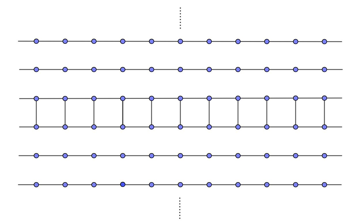
Figure 4. Case B: unperturbed situation, N=2

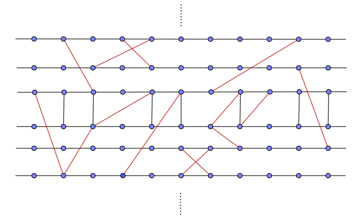
Figure 5. Case B: schematic perturbation, N=2

4.3. Coupling with a non-Hermitian model

The non-Hermitian Anderson model was first proposed for the analysis of vortex pinning in type-II superconductors [16] and has also been applied to the study of population dynamics [25]. Here, we consider a non-random version of this model. Let $\mathfrak{G}=\ell^{2}({\mathbb{Z}}_{m})$ for some $m\geq 2$, where ${\mathbb{Z}}_{m}=\mathbb{Z}/m\mathbb{Z}$, and $(e_{k})_{k\in{\mathbb{Z}}_{m}}$ its canonical orthonormal basis. Consider the operator $M$ defined by

$$Me_{k} =e^{g}e_{k-1}+e^{-g}e_{k+1},\quad k\in{\mathbb{Z}}_{m},g\in{\mathbb{R}}.$$

The operator $M$ is diagonalizable, with eigenvalues and a corresponding basis of eigenvectors given respectively by

$$\lambda_{j} =e^{g}e^{ij\theta_{m}}+e^{-g}e^{ij\theta_{m}}=2\cosh g\cos j\theta_{m}+2i\sinh g\sin j\theta_{m}\quad,\quad\theta_{m}:=\frac{2\pi}{m},$$

$$v_{j} =\sum_{k\in{\mathbb{Z}}_{m}}e^{ijk\theta_{m}}e_{k},\quad j\in{\mathbb{Z}}_{m}.$$

Similar to the previous example, if $g=0$, the operator $H_{0}$ is nothing but the discrete Laplace operator on the tube ${\mathbb{Z}}\times{\mathbb{Z}}_{m}$ (Figure 6).

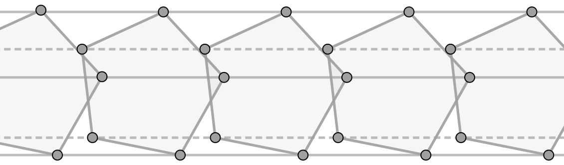
Figure 6. Tube $\mathbb{Z}\times\mathbb{Z}_{5}$

4.4. Coupling with a ${\mathcal{P}T}$-symmetric Hamiltonian

The pertinence of $\mathcal{PT}$-symmetric Hamiltonians in physics is discussed in e.g. [3, 23]. For illustrative purpose, we consider in the sequel a minimal example of a non-Hermitian, $\mathcal{PT}$-symmetric system (see [23] for details).

Let $\mathfrak{G}={\mathbb{C}}^{2}$ and $(e_{k})_{k\in\{1,2\}}$ its canonical orthonormal basis. Identifying the operators with their matrix representations in this basis, let $M$ be defined by

$$M=\kappa\sigma_{1}+i\gamma\sigma_{3}\quad\text{with}\;\;\quad\sigma_{1}=\left(\begin{array}[]{cc}0&1\\ 1&0\end{array}\right),\quad\sigma_{3}=\left(\begin{array}[]{cc}1&0\\ 0&-1\end{array}\right),$$

where $\kappa$ and $\gamma$ are non negative.

If $\kappa\neq\gamma$, direct calculations show that the eigenvalues and a corresponding basis of eigenvectors of $M$ are respectively given by:

$$\lambda_{j} =(-1)^{j+1}\sqrt{\kappa^{2}-\gamma^{2}},$$

$$v_{j} =(i\gamma+(-1)^{j+1}\sqrt{\kappa^{2}-\gamma^{2}})e_{1}+\kappa e_{2},$$

where $j\in\{1,2\}$. In this case, $M$ is diagonalizable but the eigenprojectors are not orthogonal unless $\gamma=0$.

The linear operator $M$ commutes with the antilinear operator $\mathcal{PT}$, where ${\mathcal{P}}$ stands for the linear (and unitary) operator $\sigma_{1}$ while ${\mathcal{T}}$ stands for the (antilinear) complex conjugation operator. If $\gamma<\kappa$, $\sigma(M)\subset{\mathbb{R}}$ while if $\gamma>\kappa$, $\sigma(M)\subset i{\mathbb{R}}$.

If $\kappa=\gamma>0$, the $\mathcal{PT}$ symmetry is spontaneously broken in the sense that $M$ is not diagonalizable anymore.

5. Preliminary results and proof of Proposition 2.2

5.1. Study of the resolvent of the free Hamiltonian near the spectral thresholds

The first step in our analysis is the study of the behavior of the resolvent of the free Hamiltonian $H_{0,\bullet}$ near the spectral thresholds. In order to unify the analysis for both cases (A) and (B), we introduce the operator $\widehat{\pi}_{0,\bullet}$ on $\mathfrak{G}$ defined by

$$\widehat{\pi}_{0,\bullet}:=\left\{\begin{array}[]{lll}0_{\mathfrak{G}}\;\;\text{if}\;\bullet=A\\ \pi_{0}\;\;\text{if}\;\bullet=B,\end{array}\right.$$

where we recall that $\pi_{0}$ denotes the projection onto the infinite-dimensional subspace ${\rm Ker}(M)$ in case (B). Using the fact that $M$ is diagonalizable, for any $z\in\mathbb{C}\setminus\sigma(H_{0,\bullet})$, one has

(5.1) $$(H_{0,\bullet}-z)^{-1}=\sum_{j=1}^{d}(\Delta+\lambda_{j}-z)^{-1}\otimes\pi_{j}+(\Delta-z)^{-1}\otimes\widehat{\pi}_{0,\bullet}.$$

Let us recall the following basic properties of the one-dimensional discrete Laplacian on $\ell^{2}(\mathbb{Z})$. Let $\mathcal{F}:\ell^{2}(\mathbb{Z})\to L^{2}(\mathbb{T})$ be the unitary discrete Fourier transform defined by

$$(\mathcal{F}u)(\theta)=\frac{1}{2\pi}\sum_{n\in\mathbb{Z}}e^{-in\theta}u(n),\quad u\in\ell^{2}(\mathbb{Z}),\theta\in\mathbb{T}:=\mathbb{R}/2\pi\mathbb{Z}.$$

The operator $\Delta$ is unitarily equivalent to the multiplication operator on $L^{2}(\mathbb{T})$ by the function $f:\theta\mapsto 2-2\cos(\theta)$. More precisely, one has

(5.2) $$(\mathcal{F}(\Delta u))(\theta)=f(\theta)(\mathcal{F}u)(\theta),\quad u\in\ell^{2}(\mathbb{Z}),\theta\in\mathbb{T}.$$

Hence, the operator $\Delta$ is selfadjoint in $\ell^{2}(\mathbb{Z})$ and its spectrum is absolutely continuous and coincides with the range of the function $f$, that is $\sigma(\Delta)=\sigma_{{\rm ac}}(\Delta)=[0,4]$.

For any $z\in\mathbb{C}\setminus[0,4]$, the kernel of $(\Delta-z)^{-1}$ is given by (see for instance [22])

(5.3) $$R_{0}(z;n,m)=\frac{e^{-i\theta(z)|n-m|}}{2i\sin(\theta(z))},\quad(n,m)\in\mathbb{Z}^{2},$$

where $\theta(z)$ is the unique solution to the equation $2-2\cos(\theta)=z$ lying in the region $\{\theta\in\mathbb{C};-\pi\leq{\rm Re}\,\theta\leq\pi,{\rm Im}\,\theta<0\}$.

Using this explicit representation of the kernel, we can prove the following result.

Lemma 5.1.

Let $z_{0}\in[0,4)$ and $\rho>0$. There exists $0<\varepsilon_{0}\ll 1$ such that the operator-valued function

$$D_{\varepsilon_{0}}^{*}(0)\cap\mathbb{C}_{1}\ni k\mapsto W_{-\rho}(\Delta-(z_{0}+k^{2}))^{-1}W_{-\rho}$$

admits an analytic extension to $D_{\varepsilon_{0}}^{*}(0)$ if $z_{0}=0$ and to $D_{\varepsilon_{0}}(0)$ if $z_{0}\in(0,4)$, with values in the Hilbert-Schmidt class operators $\mathfrak{S}_{2}(\ell^{2}(\mathbb{Z}))$. This extension will be denoted $R_{0}(z_{0}+k^{2})$.

In the next result, we show that the weighted resolvent of the free Hamiltonian $H_{0,\bullet}$ extends meromorphically near any $\lambda_{q}\in\mathcal{T}_{\bullet}$ and we precise the nature of its singularity at $\lambda_{q}$. Set

$$\mathcal{H}_{\bullet}:=\left\{\begin{array}[]{lll}\mathfrak{S}_{\infty}(\mathcal{H})\;\;\text{if}\;\bullet=A\\ \mathcal{B}(\mathcal{H})\;\;\text{if}\;\bullet=B.\end{array}\right.$$

Lemma 5.2.

Let $\lambda_{q}\in\mathcal{T}_{\bullet}$. There exists $0<\varepsilon_{0}\ll 1$ such that the operator-valued function

(5.4) $$D^{*}_{\varepsilon_{0}}(0)\cap\mathbb{C}_{1}\ni k\mapsto\bm{W}_{-\rho}(H_{0,\bullet}-z_{q}(k))^{-1}\bm{W}_{-\rho}$$

admits an analytic extension to $D^{*}_{\varepsilon_{0}}(0)$, with values in $\mathcal{H}_{\bullet}$, denoted $\mathcal{R}_{0,\bullet}^{(q)}(k)$. Moreover:

• If $\lambda_{q}$ is non-degenerate, then

  (5.5) $$\mathcal{R}_{0,\bullet}^{(q)}(k)-\frac{a_{-1}\otimes\pi_{q}}{k}\in{\rm Hol}\big{(}D_{\varepsilon_{0}}(0);\mathcal{H}_{\bullet}\big{)}.$$

• If $\lambda_{q}$ is degenerate such that $\lambda_{q}=\lambda_{p}+4$ for some $p\in\{1,...,d\}$, then

  (5.6) $$\mathcal{R}_{0,\bullet}^{(q)}(k)-\frac{a_{-1}\otimes\pi_{q}+b_{-1}\otimes\pi_{p}}{k}\in{\rm Hol}\big{(}D_{\varepsilon_{0}}(0);\mathcal{H}_{\bullet}\big{)}.$$

Proof.

Let us start with the proof of the first part of the result on the analytic extension. We first consider the case (A). Setting $z_{j}^{(q)}:=\lambda_{q}-\lambda_{j}$ it follows from (5.1) that

(5.7) $$\bm{W}_{-\rho}(H_{0,A}-z_{q}(k))^{-1}\bm{W}_{-\rho}=\sum_{j=1}^{d}W_{-\rho}\big{(}\Delta-(z_{j}^{(q)}+k^{2})\big{)}^{-1}W_{-\rho}\otimes\pi_{j}.$$

The above sum splits into the following two terms

(5.8) $$\bm{W}_{-\rho}(H_{0,A}-z_{q}(k))^{-1}\bm{W}_{-\rho}= \sum_{z_{j}^{(q)}\in[0,4]}W_{-\rho}\big{(}\Delta-(z_{j}^{(q)}+k^{2})\big{)}^{-1}W_{-\rho}\otimes\pi_{j}$$

$$+ \sum_{z_{j}^{(q)}\notin[0,4]}W_{-\rho}\big{(}\Delta-(z_{j}^{(q)}+k^{2})\big{)}^{-1}W_{-\rho}\otimes\pi_{j}.$$

The second term in the RHS is clearly analytic with respect to $k$ in a small neighborhood of $0$. On the other hand, by Lemma 5.1, the first term in the RHS extends to an analytic function of $k$ in $D_{\varepsilon_{0}}^{*}(0)$ for $\varepsilon_{0}>0$ small enough. The extension is clearly in $\mathfrak{S}_{\infty}(\mathcal{H})$.

Consider now the case (B). The only difference with respect to the above case comes from $q=0$. From (5.1) again one has

$$\bm{W}_{-\rho}(H_{0,B}-z_{0}(k))^{-1}\bm{W}_{-\rho}$$

$$=\sum_{j=1}^{d}W_{-\rho}\big{(}\Delta-(-\lambda_{j}+k^{2})\big{)}^{-1}W_{-\rho}\otimes\pi_{j}+\bm{W}_{-\rho}(\Delta-k^{2})^{-1}\bm{W}_{-\rho}\otimes\pi_{0}.$$

In this case, since the operator $\pi_{0}$ is not compact, the extension belongs to $\mathcal{B}(\mathcal{H})$.

Turn now to the proof of the second part of the result. We only prove (i) in case (A). The other assertion works similarly.

Recall from (5.7) that we have

$$\bm{W}_{-\rho}(H_{0,A}-z_{q}(k))^{-1} \bm{W}_{-\rho}=\sum_{j\neq q}W_{-\rho}\big{(}\Delta-(z_{j}^{(q)}+k^{2})\big{)}^{-1}W_{-\rho}\otimes\pi_{j}$$

$$+W_{-\rho}(\Delta-k^{2})^{-1}W_{-\rho}\otimes\pi_{q}.$$

Since $\lambda_{q}\neq\lambda_{j}+4$ for all $j\neq q$, it follows that $z_{j}^{(q)}\notin\{0,4\}$ for any $j\neq q\in\{1,...,d\}$. Consequently, by Lemma 5.1, the first term in the RHS of the above equation extends analytically in a small neighborhood of $0$ with values in $\mathfrak{S}_{\infty}(\mathcal{H})$. On the other hand, the kernel of the operator $W_{-\rho}(\Delta-k^{2})^{-1}W_{-\rho}$ is given by

(5.9) $$\frac{e^{-\frac{\rho}{2}|n|}}{\|e^{-\frac{\rho}{2}|\cdot|}\|_{\ell^{2}(\mathbb{Z})}}R_{0}(k;n,m)\frac{e^{-\frac{\rho}{2}|m|}}{\|e^{-\frac{\rho}{2}|\cdot|}\|_{\ell^{2}(\mathbb{Z})}},$$

where $R_{0}(k^{2};n,m)$ is defined by (5.3). One can write

(5.10) $$R_{0}(k^{2};n,m)=\frac{i}{k\sqrt{4-k^{2}}}+\frac{i(e^{i|n-m|2\arcsin\frac{k}{2}}-1)}{k\sqrt{4-k^{2}}}=\frac{i}{2k}+r(k;n,m),$$

with

$$r(k;n,m):=i\Big{(}\frac{1}{k\sqrt{4-k^{2}}}-\frac{1}{2k}\Big{)}+\frac{i(e^{i|n-m|2\arcsin\frac{k}{2}}-1)}{k\sqrt{4-k^{2}}}.$$

One easily verifies that the function $r$ extends to a holomorphic function in a small neighborhood of $0$. Therefore, putting together (5.9) and (5.10), one obtains

(5.11) $$W_{-\rho}(\Delta-k^{2})^{-1}W_{-\rho}\otimes\pi_{q}=\frac{a_{-1}\otimes\pi_{q}}{k}+\mathcal{A}(k)\otimes\pi_{q},$$

where $\mathcal{A}(k)$ acts on $\ell^{2}(\mathbb{Z})$ with kernel $W_{-\rho}(n)r(k;n,m)W_{-\rho}(m)$. This ends the proof. ∎

Remark 5.3.

In case (B), replacing one of the weight operators $\bm{W}_{-\rho}$ in (5.4) by $W_{-\rho}\otimes K$ with $K\in\mathfrak{S}_{\infty}(\mathfrak{G})$ ensures that the analytic extension holds in $\mathfrak{S}_{\infty}(\mathcal{H})$. For instance,

$$D^{*}_{\varepsilon_{0}}(0)\cap\mathbb{C}_{1}\ni k\mapsto(W_{-\rho}\otimes K)(H_{0,B}-z_{q}(k))^{-1}\bm{W}_{-\rho}$$

admits an analytic extension to $D^{*}_{\varepsilon_{0}}(0)$, with values in $\mathfrak{S}_{\infty}(\mathcal{H})$.

5.2. Proof of Proposition 2.2

The proof is a consequence of Lemma 5.2 and the analytic Fredholm extension Theorem. From the resolvent identity

$$(H_{\omega,\bullet}-z)^{-1}(I+\omega V(H_{0,\bullet}-z)^{-1})=(H_{0,\bullet}-z)^{-1},$$

it follows that

(5.12) $$\bm{W}_{-\rho}(H_{\omega,\bullet}-z_{q}(k))^{-1}\bm{W}_{-\rho}=\bm{W}_{-\rho}(H_{0,\bullet}-z_{q}(k))^{-1}\bm{W}_{-\rho}\big{(}I+\mathcal{P}_{\omega,\bullet}(z_{q}(k))\big{)}^{-1},$$

where

(5.13) $$\mathcal{P}_{\omega,\bullet}(z):=\omega\bm{W}_{\rho}V(H_{0,\bullet}-z)^{-1}\bm{W}_{-\rho}.$$

Lemma 5.2 implies that there exists $\varepsilon_{0}>0$ such that the operator-valued function $k\mapsto\mathcal{P}_{\omega,\bullet}(z_{q}(k))$ defined by (5.13) extends to an analytic function in $D^{*}_{\varepsilon_{0}}(0)$. In case (A), Lemma 5.2 again ensures that this extension is with values in $\mathfrak{S}_{\infty}(\mathcal{H})$. On the other hand, under Assumption 2.1 (B), assume for instance that $V\geq 0$. Then, there exists a bounded operator $\mathcal{U}$ such that $U=\bm{W}_{-\rho}\mathcal{U}\bm{W}_{-\rho}$ and it follows that

$$\mathcal{P}_{\omega,B}(z_{q}(k)) =\omega\bm{W}_{\rho}V(H_{0,B}-z_{q}(k))^{-1}\bm{W}_{-\rho}$$

$$=\omega\bm{W}_{\rho}(1\otimes K^{\ast})\bm{W}_{-\rho}\mathcal{U}\bm{W}_{-\rho}(1\otimes K)(H_{0,B}-z_{q}(k))^{-1}\bm{W}_{-\rho}$$

$$=\omega(1\otimes K^{\ast})\mathcal{U}(W_{-\rho}\otimes K)(H_{0,B}-z_{q}(k))^{-1}\bm{W}_{-\rho}.$$

According to Remark 5.3, $(W_{-\rho}\otimes K)(H_{0,B}-z_{q}(k))^{-1}\bm{W}_{-\rho}$ extends to an analytic extension in a small neighborhood of $0$ with values in $\mathfrak{S}_{\infty}(\mathcal{H})$. Since the operator $(1\otimes K^{\ast})\mathcal{U}$ is bounded, it follows that the analytic extension of $\mathcal{P}_{\omega,B}(z_{q}(k))$ is also with values in $\mathfrak{S}_{\infty}(\mathcal{H})$. Therefore the analytic Fredholm theorem ensures that

$$D^{*}_{\varepsilon_{0}}(0)\cap\mathbb{C}_{1}\ni k\mapsto\big{(}I+\mathcal{P}_{\omega,\bullet}(z_{q}(k))\big{)}^{-1}$$

admits a meromorphic extension to $D^{*}_{\varepsilon_{0}}(0)$. We use the same notation for the extended operator. Hence, the operator-valued function $k\mapsto\bm{W}_{-\rho}(H_{\omega,\bullet}-z_{q}(k))^{-1}\bm{W}_{-\rho}$ extends to a meromorphic function of $k\in D^{*}_{\varepsilon_{0}}(0)$. This ends the proof of Propositions 2.2.

6. Proofs Theorems 3.1

Let us start with the following preliminary results which precise the nature of the singularity of the meromorphic extension of the weighted resolvent at the thresholds. Recall that $a_{-1}$ is the operator in $\ell^{2}(\mathbb{Z})$ with kernel $\frac{i}{2}W_{-\rho}(n)W_{-\rho}(m)$ and we introduce the operator $b_{-1}$ in $\ell^{2}(\mathbb{Z})$ with kernel $-\frac{(-1)^{n+m}}{2}W_{-\rho}(n)W_{-\rho}(m)$.

Proposition 6.1.

Let $\lambda_{q}\in\mathcal{T}_{\bullet}$ be such that $\lambda_{q}\neq\zeta_{p}$ for all $p\neq q$. There exists $\varepsilon_{0}>0$ small enough such that for $k\in D^{*}_{\varepsilon_{0}}(0)$ the following statements hold:

• If $\lambda_{q}=\lambda_{q}$ then

  (6.1) $$\bm{W}_{-\rho}(H_{0,\bullet}-z_{q}(k))^{-1}\bm{W}_{-\rho}-\frac{a_{-1}\otimes\pi_{q}}{k}\in\text{Hol}\,\big{(}D_{\varepsilon_{0}}(0);\mathfrak{E}\big{)}.$$

• If $\lambda_{q}=\lambda_{q}+4$ then

  (6.2) $$\bm{W}_{-\rho}(H_{0,\bullet}-z_{q}(k))^{-1}\bm{W}_{-\rho}-\frac{b_{-1}\otimes\pi_{q}}{k}\in\text{Hol}\,\big{(}D_{\varepsilon_{0}}(0);\mathfrak{E}\big{)}.$$

  Here $\mathfrak{E}$ is equals to $\mathcal{S}_{\infty}(\ell^{2}(\mathbb{Z})\otimes\mathfrak{G})$ in the case $\bullet=A$ and equals to $\mathcal{B}(\ell^{2}(\mathbb{Z};\mathcal{G}))$ in the case $\bullet=B$.

Proof.

Let us start with the case (A). Suppose that $\lambda_{q}=\lambda_{q}$ and recall from (5.1) that we have

$$\bm{W}_{-\rho}(H_{0,A}-z_{q}(k))^{-1} \bm{W}_{-\rho}=\sum_{j\neq q}W_{-\rho}\big{(}\Delta-(\lambda_{q}-\lambda_{j}+k^{2})\big{)}^{-1}W_{-\rho}\otimes\pi_{j}$$

$$+W_{-\rho}\big{(}\Delta-k^{2}\big{)}^{-1}W_{-\rho}\otimes\pi_{q}.$$

Since $\lambda_{q}\neq\lambda_{j}+4$ for all $j\neq q$ it follows that $\lambda_{q}-\lambda_{j}\notin\{0,4\}$ for any $j\neq q\in\{1,...,d\}$. Consequently, by Lemma 5.1, the first term in the RHS of the above equation extends analytically in a small neighborhood of $0$. On the other hand, taking the Laurent expansion of $k\mapsto W_{-\rho}\big{(}\Delta-k^{2}\big{)}^{-1}W_{-\rho}\otimes\pi_{q}$ near $k=0$ using the fact that the kernel of $\big{(}\Delta-k^{2}\big{)}^{-1}$ is given by according to (5.3) one gets

$$W_{-\rho}\big{(}\Delta-k^{2}\big{)}^{-1}W_{-\rho}\otimes\pi_{q}-\frac{1}{k}a_{-1}\otimes\pi_{q}\in\text{Hol}\,\big{(}D_{\varepsilon_{0}}(0);\mathcal{S}_{\infty}(\ell^{2}(\mathbb{Z})\otimes\mathfrak{G})\big{)},$$

which proves the claim of (i). The proof of (ii) is similar except that in this case the kernel of $(\Delta-(4+k^{2}))^{-1}$ is given by $\frac{-(-1)^{n+m}}{2}W_{-\rho}(n)W_{-\rho}(m)$.

Consider now the case (B) and suppose that $\lambda_{q}=\lambda_{q}$. From (5.1) we have

$$\bm{W}_{-\rho}(H_{0,B}-z_{q}(k))^{-1} \bm{W}_{-\rho}=\sum_{j=1}^{d}W_{-\rho}\big{(}\Delta-(\lambda_{q}-\lambda_{j}+k^{2})\big{)}^{-1}W_{-\rho}\otimes\pi_{j}$$

$$+W_{-\rho}\big{(}\Delta-(\lambda_{q}+k^{2})\big{)}^{-1}W_{-\rho}\otimes\pi_{0}.$$

Assume first that $\lambda_{q}\neq 0$. It follows from Lemma 5.1 that the second term in the RHS of the above equation extends analytically in a small neighborhood of $0$. The first term can be treated as above and then we get the claim. The case $\lambda_{q}=0$ follows again from Lemma 5.1 and the above analysis. ∎

7. Proofs of Theorems 3.1 and 3.2

7.1. Proof of part (i) of Theorem 3.1

Let $\lambda_{q}\in\mathcal{T}_{A}$ be a fixed threshold and assume that $\lambda_{q}$ is non-degenerate in the sense of Definition 2.1.

According to Lemma 5.2, there exists $\varepsilon_{0}>0$ and an analytic function $\mathcal{G}$ in $D_{\varepsilon_{0}}(0)$ with values in $\mathfrak{S}_{\infty}(\mathcal{H})$ such that for all $k\in D_{\varepsilon_{0}}^{*}(0)$ we have

(7.1) $$\mathcal{R}_{0,A}^{(q)}(k)=\frac{a_{-1}\otimes\pi_{q}}{k}+\mathcal{G}(k).$$

It follows from equation (5.12) that for all $k\in D_{\varepsilon_{0}}^{*}(0)$,

(7.2) $$\mathcal{R}_{\omega,A}^{(q)}(k)=\Big{(}\frac{a_{-1}\otimes\pi_{q}}{k}+\mathcal{G}(k)\Big{)}\left[I+\mathcal{P}_{\omega,A}(z_{q}(k))\right]^{-1},$$

where $\mathcal{P}_{\omega,A}(z_{q}(k))$ is defined by (5.13). More precisely, one has

(7.3) $$\left[I+\mathcal{P}_{\omega,A}(z_{q}(k))\right]^{-1}=\big{(}I+\omega{V}_{\rho}\mathcal{R}_{0,A}^{(q)}(k)\big{)}^{-1}.$$

Since $\mathcal{G}$ is analytic near $0$, it follows that for $|\omega|$ small enough, the operator-valued function $I+\omega{V}_{\rho}\mathcal{G}(k)$ is invertible. Using (7.1), one writes

(7.4) $$\left[I+\mathcal{P}_{\omega,A}(z_{q}(k))\right]^{-1}=\Big{(}I+\frac{\omega}{k}\mathcal{L}_{\omega}(k)\Big{)}^{-1}\left(I+\omega{V}_{\rho}\mathcal{G}(k)\right)^{-1},$$

where $\mathcal{L}_{\omega}(k)$ is the operator in $\mathcal{H}$ defined by

$$\mathcal{L}_{\omega}(k):=\left(I+\omega{V}_{\rho}\mathcal{G}(k)\right)^{-1}{V}_{\rho}(a_{-1}\otimes\pi_{q}).$$

Putting together (7.2) and (7.4), we obtain, for all $k\in D_{\varepsilon_{0}}^{*}(0)$,

(7.5) $$\mathcal{R}_{\omega,A}^{(q)}(k)=\Big{(}\frac{a_{-1}\otimes\pi_{q}}{k}+\mathcal{G}(k)\Big{)}\Big{(}I+\frac{\omega}{k}\mathcal{L}_{\omega}(k)\Big{)}^{-1}\left(I+\omega{V}_{\rho}\mathcal{G}(k)\right)^{-1}.$$

Then, the poles of $k\mapsto\mathcal{R}_{\omega,A}^{(q)}(k)$ near $0$ coincide with those of the operator-valued function

(7.6) $$k\mapsto J_{\omega}(k):=\Big{(}\frac{a_{-1}\otimes\pi_{q}}{k}+\mathcal{G}(k)\Big{)}\Big{(}I+\frac{\omega}{k}\mathcal{L}_{\omega}(k)\Big{)}^{-1}.$$

We shall make use of the following elementary result whose proof is omitted.

Lemma 7.1.

Let $\mathcal{K}$ be a Hilbert space and consider two linear operators $A,\Pi:\mathcal{K}\to\mathcal{K}$ such that $\Pi^{2}=\Pi$ and $A\Pi=A$. Then, $I+A$ is invertible if and only if $\Pi(I+A)\Pi:{\rm Ran}\,\Pi\to{\rm Ran}\,\Pi$ is invertible, and in this case one has

$$(I+A)^{-1}=(I-\widetilde{\Pi}A\Pi)B^{-1}+\widetilde{\Pi},$$

where $\widetilde{\Pi}:=I-\Pi$ and $B^{-1}:=(\Pi(I+A)\Pi)^{-1}\oplus 0$ with respect to the decomposition $\mathcal{K}={\rm Ran}\,\Pi\oplus{\rm Ran}\,\widetilde{\Pi}$.

Let $\Pi_{q}$ be the projection on $\mathcal{H}$ defined by (3.3). Applying the above result with $A=\frac{\omega}{k}\mathcal{L}_{\omega}(k)$ and $\Pi=\Pi_{q}$, we get

$$\Big{(}I+\frac{\omega}{k}\mathcal{L}_{\omega}(k)\Big{)}^{-1}=\Big{(}I-\frac{\omega}{k}\widetilde{\Pi}_{q}\mathcal{L}_{\omega}(k)\Pi_{q}\Big{)}\biggl{(}\left(\Pi_{q}\left(I+\frac{\omega}{k}\mathcal{L}_{\omega}(k)\right)\Pi_{q}\right)^{-1}\oplus 0\biggr{)}+\widetilde{\Pi}_{q}.$$

Here, $\widetilde{\Pi}_{q}:=I-\Pi_{q}$. Therefore, a straightforward computation yields

$$J_{\omega}(k) =\left(\frac{i}{2}\Pi_{q}-\omega\mathcal{G}(k)\Big{(}\frac{k}{\omega}-\widetilde{\Pi}_{q}\mathcal{L}_{\omega}(k)\Pi_{q}\Big{)}\right)\big{(}\left[\Pi_{q}\left(k+\omega\mathcal{L}_{\omega}(k)\right)\Pi_{q}\right]^{-1}\oplus 0\big{)}$$

$$+\mathcal{G}(k)\widetilde{\Pi}_{q}.$$

Since $\left[\Pi_{q}\left(k+\omega\mathcal{L}_{\omega}(k)\right)\Pi_{q}\right]^{-1}:{\rm Ran}\,\Pi_{q}\to{\rm Ran}\,\Pi_{q}$, it follows that the operator $\left[\Pi_{q}\left(k+\omega\mathcal{L}_{\omega}(k)\right)\Pi_{q}\right]^{-1}\oplus 0$ is stable by $\Pi_{q}:\mathcal{H}\to\mathcal{H}$. Consequently,

(7.7) $$\begin{split}J_{\omega}(k)&=\left(\frac{i}{2}-\omega\mathcal{G}(k)\Big{(}\frac{k}{\omega}-\widetilde{\Pi}_{q}\mathcal{L}_{\omega}(k)\Pi_{q}\Big{)}\right)\big{(}\left[\Pi_{q}\left(k+\omega\mathcal{L}_{\omega}(k)\right)\Pi_{q}\right]^{-1}\oplus 0\big{)}\\ &+\mathcal{G}(k)\widetilde{\Pi}_{q}.\end{split}$$

Using the analyticity of $\mathcal{G}$ and $\mathcal{L}_{\omega}$ near $0$, one sees that $\frac{i}{2}-\omega\mathcal{G}(k)\big{(}\frac{k}{\omega}-\widetilde{\Pi}_{q}\mathcal{L}_{\omega}(k)\Pi_{q}\big{)}$ is invertible for $|k|$ of order of $|\omega|\ll 1$ small enough. Therefore, we conclude that the poles near $0$ of $J_{\omega}$ are the same to those of the operator-valued function

$$k\mapsto\left(\Pi_{q}\left(k+\omega\mathcal{L}_{\omega}(k)\right)\Pi_{q}\right)^{-1}:{\rm Ran}\,\Pi_{q}\to{\rm Ran}\,\Pi_{q}.$$

Let $M_{\omega}(k)$ be the matrix of the operator $\Pi_{q}\left(k+\omega\mathcal{L}_{\omega}(k)\right)\Pi_{q}:{\rm Ran}\,\Pi_{q}\to{\rm Ran}\,\Pi_{q}$. We have

$$\Pi_{q}\left(k+\omega\mathcal{L}_{\omega}(k)\right)\Pi_{q} =k\Pi_{q}+\omega\Pi_{q}\left(I+\omega{V}_{\rho}\mathcal{G}(k)\right)^{-1}{V}_{\rho}(a_{-1}\otimes\pi_{q})\Pi_{q}$$

(7.8) $$=k\Pi_{q}+\frac{i}{2}\omega\Pi_{q}{V}_{\rho}\Pi_{q}+\omega^{2}\Pi_{q}S_{\omega}(k)\Pi_{q},$$

where $k\mapsto S_{\omega}(k):=\frac{i}{2}\sum_{n\geq 1}(-1)^{n}\omega^{n-1}({V}_{\rho}\mathcal{G}(k))^{n}{V}_{\rho}$ is an operator-valued function which is analytic near $k=0$ for $|\omega|>0$ small enough and $\|S_{\omega}(k)\|=\mathcal{O}(1)$ uniformly w.r.t. $k$.

The usual expansion formula for the determinant allows to write

$${\rm det}(M_{\omega}(k))=\omega^{\nu_{q}}\biggl{(}\prod_{j=1}^{r}\Big{(}\frac{k}{\omega}+\bm{\alpha}_{j}^{(q)}\Big{)}^{m_{q,j}}+\omega s_{\omega}(k)\biggr{)},$$

with $\bm{\alpha}_{j}^{(q)}:=\frac{i}{2}\alpha_{j}^{(q)}$, where $\{{\alpha_{j}^{(q)}}\}_{j=1}^{r}$ are the distinct eigenvalues of $E_{q}:=\Pi_{q}{V}_{\rho}\Pi_{q}:{\rm Ran}\,\Pi_{q}\to{\rm Ran}\,\Pi_{q}$ and $s_{\omega}$ is an analytic scalar-valued function satisfying

(7.9) $$|s_{\omega}(k)|\leq C_{0},$$

for some constant $C_{0}>0$ independent of $k$ and $\omega$. We are therefore led to study the roots of the equation

(7.10) $$\prod_{j=1}^{r}\Big{(}\frac{k}{\omega}+\bm{\alpha}_{j}^{(q)}\Big{)}^{m_{q,j}}+\omega s_{\omega}(k)=0.$$

On the one hand, by a simple contradiction argument one shows that all the roots of the above equation satisfy (3.5). On the other hand, let $j_{0}\in\{1,...,r\}$ and let $C>0$ be a constant independent of $k$ and $\omega$. We set

$\delta_{j_{0},C}:=C|\omega|^{1+\frac{1}{m_{q,j_{0}}}}.$

There exists a constant $C^{\prime}>0$ such that for any $k\in\partial D_{\delta_{j_{0},C}}(-\bm{\alpha}_{j_{0}}\omega)$, one has

$$\prod_{j=1,j\neq j_{0}}^{r}\Big{|}\frac{k}{\omega}+\bm{\alpha}_{j}^{(q)}\Big{|}^{m_{q,j}}\geq C^{\prime}.$$

Consequently,

$$\prod_{j=1}^{r}\Big{|}\frac{k}{\omega}+\bm{\alpha}_{j}^{(q)}\Big{|}^{m_{q,j}}\geq CC^{\prime}|\omega|>|\omega s_{\omega}(k)|,\quad\forall k\in\partial D_{\delta_{j_{0},C}}(-\bm{\alpha}_{j_{0}}\omega),$$

where $C>0$ is chosen such that $CC^{\prime}>C_{0}$, with $C_{0}$ given by (7.9).

Since both terms in (7.10) are analytic functions of $k$ near $k=0$, it follows by Rouché Theorem that for $|\omega|$ small, ${\rm det}(M_{\omega}(k))$ admits exactly $m_{q,j_{0}}$ zeros in $D_{\delta_{j_{0},C}}(-\bm{\alpha}_{j_{0}}\omega)$, counting multiplicities. This ends the proof of statement (i).

7.2. Proof of part (ii) of Theorem 3.1

Fix $q\in\{1,...,d\}$. Equation (3.5) implies that in variable $k$, the resonances of $H_{\omega,A}$ are distributed in “clusters” around the points $-\frac{i}{2}\omega\alpha_{j}^{(q)}$, $j\in\{1,...,r\}$. Fix $j\in\{1,...,r\}$ and let $C>0$ and $1<\delta<1+\frac{1}{m_{q,j}}$ so that the disk $D_{C|\omega|^{\delta}}(-\frac{i}{2}\omega\alpha_{j}^{(q)})$ contains all the resonances of the j-th cluster and only them. Set $\Gamma_{j}:=\partial D_{C|\omega|^{\delta}}(-\frac{i}{2}\omega\alpha_{j}^{(q)})$. We will show that

(7.11) $${\rm rank}\frac{1}{2i\pi}\oint_{\Gamma_{j}}\mathcal{R}^{(q)}_{\omega,A}(k)dk={\rm rank}\frac{1}{2i\pi}\oint_{\Gamma_{j}}(k\Pi_{q}+\frac{i}{2}\omega\Pi_{q}{V}_{\rho}\Pi_{q})^{-1}\,dk.$$

Since the RHS is equal to the multiplicity of $-\frac{i}{2}\omega\alpha_{j}^{(q)}$, part ii) of Theorem 3.1 follows.

Equality (7.11) is a consequence of the following Lemma and standard arguments (see for instance [27, Page 14] and Lemma 4.1 of [20, Chapter 1]).

Lemma 7.1.

As $|\omega|\to 0$, one has

1. $\Big{\|}\oint_{\Gamma_{j}}\mathcal{R}^{(q)}_{\omega,A}(k)-\left(k\Pi_{q}+\frac{i}{2}\omega\Pi_{q}{V}_{\rho}\Pi_{q}\right)^{-1}\,dk\Big{\|}=o(1)$.

2. $\Big{\|}\left(\frac{1}{2i\pi}\oint_{\Gamma_{j}}\mathcal{R}^{(q)}_{\omega,A}(k)dk\right)^{2}-\frac{1}{2i\pi}\oint_{\Gamma_{j}}\mathcal{R}^{(q)}_{\omega,A}(k)dk\Big{\|}=o(1).$

Proof.

We simplify the notations by putting

$$\mathcal{A}_{0}(k):=k\Pi_{q}+\frac{i}{2}\omega\Pi_{q}{V}_{\rho}\Pi_{q}\quad\text{and}\quad\mathcal{A}(k):=\Pi_{q}\left(k+\omega\mathcal{L}_{\omega}(k)\right)\Pi_{q}$$

as operators acting from ${\rm Ran}\,\Pi_{q}\to{\rm Ran}\,\Pi_{q}$. Using (7.5), (7.6) and (7.7), one gets

(7.12) $$\oint_{\Gamma_{j}}\mathcal{R}^{(q)}_{\omega,A}(k)dk=\oint_{\Gamma_{j}}T_{\omega}(k)(\mathcal{A}(k)^{-1}\oplus 0)U_{\omega}(k)dk,$$

where $T_{\omega}(k)=I+\omega\widetilde{T}_{\omega}(k)$ and $U_{\omega}(k)=I+\omega\widetilde{U}_{\omega}(k)$ are holomorphic operator-valued functions in $k$ and uniformly bounded inside $\Gamma_{j}$. One writes

(7.13) $$\begin{split}T_{\omega}(k)(\mathcal{A}(k)^{-1}&\oplus 0)U_{\omega}(k)=\mathcal{A}(k)^{-1}\oplus 0+\omega\widetilde{T}_{\omega}(k)(\mathcal{A}(k)^{-1}\oplus 0)\\ &+\omega(\mathcal{A}(k)^{-1}\oplus 0)\widetilde{U}_{\omega}(k)+\omega^{2}\widetilde{T}_{\omega}(k)(\mathcal{A}(k)^{-1}\oplus 0)\widetilde{U}_{\omega}(k).\end{split}$$

On the other hand, from (7.1), one has for any $k\in\Gamma_{j}$,

(7.14) $$\mathcal{A}(k)=\mathcal{A}_{0}(k)\big{(}I+\omega^{2}\mathcal{A}_{0}(k)^{-1}\widetilde{S}_{\omega}(k)\big{)},$$

with $\widetilde{S}_{\omega}(k):=\Pi_{q}S_{\omega}(k)\Pi_{q}$. The fact that $M$ and $V$ are selfadjoint in $\mathcal{H}$ implies that $\Pi_{q}{V_{\rho}}\Pi_{q}$ is selfadjoint. Thus, for any $k\in\Gamma_{j}$, we have

(7.15) $$\|\mathcal{A}_{0}(k)^{-1}\|=\|(k\Pi_{q}+\frac{i}{2}\omega\Pi_{q}{V}_{\rho}\Pi_{q})^{-1}\|=\frac{1}{{\rm dist}(k,\sigma(-\frac{i}{2}\omega\Pi_{q}{V}_{\rho}\Pi_{q}))}=\mathcal{O}(|\omega|^{-\delta}).$$

Therefore, $\|\big{(}I+\omega^{2}\mathcal{A}_{0}(k)^{-1}\widetilde{S}_{\omega}(k)\big{)}^{-1}\|=\mathcal{O}(1)$ for $|\omega|$ small enough uniformly w.r.t. $k\in\Gamma_{j}$. It follows from (7.14) that we have

(7.16) $$\begin{split}\Big{\|}\oint_{\Gamma_{j}}&\,\omega\widetilde{T}_{\omega}(k)(\mathcal{A}(k)^{-1}\oplus 0)\,dk\Big{\|}\\ &\leq{\rm Cst.}\,|\omega||\omega|^{\delta}\int_{0}^{2\pi}\|\mathcal{A}_{0}(k_{\omega}(t))^{-1}\|\,dt=\mathcal{O}(|\omega|),\end{split}$$

where $k_{\omega}(t):=-\frac{i}{2}\omega\alpha_{j}^{(q)}+e^{it}C|\omega|^{\delta}$. The integral over $\Gamma_{j}$ of each one of the two last terms in the RHS of (7.13) can be estimated in the same way and we obtain

(7.17) $$\begin{split}&\Big{\|}\oint_{\Gamma_{j}}\omega(\mathcal{A}(k)^{-1}\oplus 0)\widetilde{U}_{\omega}(k)dk\Big{\|}=\mathcal{O}(|\omega|),\\ &\Big{\|}\oint_{\Gamma_{j}}\omega^{2}\widetilde{T}_{\omega}(k)(\mathcal{A}(k)^{-1}\oplus 0)\widetilde{U}_{\omega}(k)dk\Big{\|}=\mathcal{O}(|\omega|).\end{split}$$

Now, using (7.15) again, we get $\|\big{(}I+\omega^{2}\mathcal{A}_{0}(k)^{-1}\widetilde{S}_{\omega}(k)\big{)}^{-1}-I\|=\mathcal{O}(|\omega|^{2-\delta})$, which yields

$$\Big{\|}\oint_{\Gamma_{j}}\mathcal{A}(k)^{-1} -\mathcal{A}_{0}(k)^{-1}\,dk\Big{\|}$$

$$=\Big{\|}\oint_{\Gamma_{j}}\big{[}(I+\omega^{2}\mathcal{A}_{0}(k)^{-1}\widetilde{S}_{\omega}(k))^{-1}-I\big{]}\mathcal{A}_{0}(k)^{-1}\,dk\Big{\|}$$

(7.18) $$\leq{\rm Cst.}\,|\omega|^{2-\delta}|\omega|^{\delta}\int_{0}^{2\pi}\|\mathcal{A}_{0}(k_{\omega}(t))^{-1}\|\,dt=\mathcal{O}(|\omega|^{2-\delta}).$$

Putting together (7.12), (7.13), (7.16), (7.17) and (7.2) we get statement a).

Let us now prove statement $b)$. We set ${\widetilde{\Gamma}}_{j}(t)=\{-\frac{i}{2}\omega\alpha_{j}^{(q)}+e^{-it}\varepsilon|\omega|^{\delta},t\in[0,2\pi]\}$ with $0<\epsilon<C$ independent of $\omega$. For $k\in\Gamma_{j}$ and $\widetilde{k}\in\widetilde{\Gamma}_{j}$, using (7.13) and proceeding as above, one obtains

(7.19) $$\Big{\|}\oint_{\Gamma_{j}}\oint_{\widetilde{\Gamma}_{j}}\mathcal{R}^{(q)}_{\omega,A}(k)\mathcal{R}^{(q)}_{\omega,A}(\widetilde{k})-\mathcal{A}(k)^{-1}\mathcal{A}(\widetilde{k})^{-1}d\widetilde{k}dk\Big{\|}=\mathcal{O}(|\omega|).$$

Next, from the resolvent identity one writes

(7.20) $$\mathcal{A}(k)^{-1}\mathcal{A}({\widetilde{k}})^{-1}=\frac{\mathcal{A}(k)^{-1}}{{\widetilde{k}}-k}-\frac{\mathcal{A}({\widetilde{k}})^{-1}}{{\widetilde{k}}-k}-\omega^{2}\mathcal{A}({k})^{-1}\frac{(\widetilde{S}_{\omega}({\widetilde{k}})-(\widetilde{S}_{\omega}({k}))}{{\widetilde{k}}-k}\mathcal{A}({\widetilde{k}})^{-1}.$$

Further, since $\epsilon<C$, then for $k\in\Gamma_{j}$ the map $\widetilde{k}\mapsto\frac{1}{\widetilde{k}-k}$ is holomorphic inside $\widetilde{\Gamma}_{j}$ so that $\oint_{{\widetilde{\Gamma}}_{j}}\frac{d\widetilde{k}}{\widetilde{k}-k}=0$. Thus, one gets

(7.21) $$\oint_{\Gamma_{j}}\oint_{{\widetilde{\Gamma}}_{j}}\frac{\mathcal{A}(k)^{-1}}{{\widetilde{k}}-k}d{\widetilde{k}}dk-\oint_{{\Gamma}_{j}}\oint_{{\widetilde{\Gamma}}_{j}}\frac{\mathcal{A}({\widetilde{k}})^{-1}}{{\widetilde{k}}-k}d{\widetilde{k}}dk=2i\pi\oint_{\Gamma_{j}}{\mathcal{A}(k)^{-1}}dk.$$

Using the fact that $\|\big{(}I+\omega^{2}\mathcal{A}_{0}(k)^{-1}\widetilde{S}_{\omega}(k)\big{)}^{-1}\|=\mathcal{O}(1)$ as above together with (7.14), we obtain by setting $\widetilde{k}_{\omega}(t^{\prime}):=-\frac{i}{2}\omega\alpha_{j}^{(q)}+e^{-it^{\prime}}\varepsilon|\omega|^{\delta}$ for $t^{\prime}\in[0,2\pi]$,

$$|\omega|^{2}\Big{\|}\oint_{\Gamma_{j}}\oint_{{\widetilde{\Gamma}}_{j}} \mathcal{A}({k})^{-1}\frac{(\widetilde{S}_{\omega}({\widetilde{k}})-(\widetilde{S}_{\omega}({k}))}{{\widetilde{k}}-k}\mathcal{A}({\widetilde{k}})^{-1}d{\widetilde{k}}d{k}\Big{\|}$$

$$\leq {\rm Cst.}\,|\omega|^{2}|\omega|^{2\delta}\int_{0}^{2\pi}\int_{0}^{2\pi}\frac{\|\mathcal{A}_{0}({k_{\omega}(t)})^{-1}\|\|\mathcal{A}_{0}({\widetilde{k}_{\omega}(t^{\prime})})^{-1}\|}{{|\widetilde{k}_{\omega}(t^{\prime})}-k_{\omega}(t)|}dt^{\prime}dt$$

$$\leq {\rm Cst.}\,|\omega|^{2}|\omega|^{2\delta}\int_{0}^{2\pi}\int_{0}^{2\pi}\frac{|\omega|^{-2\delta}}{|\omega|^{\delta}}dt^{\prime}dt$$

(7.22) $$= \mathcal{O}(|\omega|^{2-\delta}).$$

Putting together (7.19)-(7.2) and using (7.13) and (7.16), we get statement $b)$. ∎

7.3. Proof of of Theorem 3.2

The proof can be performed in a similar manner as that of (i) of Theorem 3.1. The only difference is to define the operator $\mathcal{L}_{\omega}(k)$ by

$$\mathcal{L}_{\omega}(k)=\left(I+\omega{V}_{\rho}\mathcal{G}(k)\right)^{-1}{V}_{\rho}\left(a_{-1}\otimes\pi_{q}+b_{-1}\otimes\pi_{p}\right)$$

to get the analogous equation of (7.5) in this case. Then, Lemma 7.1 can be applied with $\Pi=\Pi_{q,p}$ and (7.7) is also obtained. The rest of the proof is similar.

8. Proof of Theorem 3.4

8.1. Resonances as characteristic values

We start this section by giving an alternative definition of the multiplicity of a resonance. Our first task will be to show that this new definition coincides with the one given in (2.4).

To begin with, let us recall some definitions and results on characteristic values. For more details, one refers to [13] and the book [14, Section 4]. Let $\mathscr{U}$ be a neighborhood of a fixed point $w\in\mathbb{C}$, and $F:\mathscr{U}\setminus\{w\}\longrightarrow{\mathcal{B}}(\mathcal{K})$ be a holomorphic operator-valued function. The function $F$ is said to be finite meromorphic at $w$ if its Laurent expansion at $w$ has the form

$F(z)=\sum_{n=m}^{+\infty}(z-w)^{n}A_{n},\quad m>-\infty,$

where (if $m<0$) the operators $A_{m},\ldots,A_{-1}$ are of finite rank.

Assume that the set $\mathscr{U}$ is open and connected, $F$ is finite meromorphic and Fredholm at each point of $\mathscr{U}$, and there exists $w_{0}\in\mathscr{U}$ such that $F(w_{0})$ is invertible. Then, there exists a closed and discrete subset $Z^{\prime}$ of $\mathscr{U}$ such that $F(z)$ is invertible for each $z\in\mathcal{D}\backslash Z^{\prime}$ and

$$F^{-1}:\mathscr{U}\backslash Z^{\prime}\longrightarrow{\rm GL}(\mathcal{K})$$

is finite meromorphic and Fredholm at each point of $\mathscr{U}$ [14, Proposition 4.1.4].

Definition 8.1.

The points of $Z^{\prime}$ where the function $F$ or $F^{-1}$ is not holomorphic are called the characteristic values of $F$. The index of $F$ with respect to the contour $\partial\Omega$ is defined by

(8.1) $$Ind_{\partial\Omega}\hskip 1.42262ptF:=\frac{1}{2i\pi}\textup{Tr}\oint_{\partial\Omega}F^{\prime}(z)F(z)^{-1}dz,$$

where $\partial\Omega$ is the boundary of a connected domain $\Omega\subseteq\mathcal{D}$ not intersecting $Z^{\prime}$. This number is actually an integer (see section [14, Section 4]).

Now, let $\lambda_{q}\in\mathcal{T}_{\bullet}$ be fixed so that $z_{q}(k)$ is defined by (2.1). It follows from identity (5.12) and Lemma 5.2 that $z_{0}=z_{q}(k_{0})\in{\rm Res}(H_{\omega,\bullet})\setminus\mathcal{T}_{\bullet}$ if and only if $k_{0}\in D^{*}_{\varepsilon_{0}}(0)$ is a characteristic value of the operator-valued function $I+\mathcal{P}_{\omega,\bullet}(z_{q}(\cdot))$, where $\mathcal{P}_{\omega,\bullet}(\cdot)$ is defined by (5.13).

Definition 8.2.

For $z_{0}\in{\rm Res}(H_{\omega,\bullet})$, we define

(8.2) $$\textup{mult}_{T}(z_{0}):=Ind_{\gamma_{z}}\,\big{(}I+\mathcal{P}_{\omega,\bullet}(z_{q}(\cdot))\big{)}.$$

Here, $\gamma_{z}$ is a positively oriented circle chosen sufficiently small so that $k_{0}$ is the only characteristic value enclosed by $\gamma_{z}$.

The following result states that both definitions (8.2) and (2.4) of the multiplicity of a resonance coincide.

Lemma 8.3.

Let Assumption 2.1 $(\bullet)$ holds and let $z_{0}\in{\rm Res}(H_{\omega,\bullet})$. Then, one has

$$\textup{mult}_{T}(z_{0})=\textup{mult}(z_{0}).$$

Proof.

This result is a consequence of Proposition 9.1 applied to $P=H_{\omega,\bullet}$, $Q=H_{0,\bullet}$ and $S=\omega V$. Set $B:=\mathcal{H}=\ell^{2}(\mathbb{Z})\otimes\mathfrak{G}$, $B_{0}:=\ell^{2}_{\rho}(\mathbb{Z})\otimes\mathfrak{G}$ and $B_{1}:=\ell^{2}_{-\rho}(\mathbb{Z})\otimes\mathfrak{G}$, where $\ell^{2}_{\pm\rho}(\mathbb{Z}):=\{u:\mathbb{Z}\to\mathbb{C}:\sum_{n\in\mathbb{Z}}|u(n)|^{2}e^{\pm\rho|n|}<\infty\}$. It is standard to see that $B_{0}$ is dense in $B$, $B$ is dense in $B_{1}$ and that the corresponding inclusions are continuous. From Assumption 2.1 ($\bullet$), the operator $V$ is bounded. Then, Conditions (I) and (II) are satisfied since $H_{0,\bullet}+\omega V$ is bounded. Thus, all the requirements of Proposition 9.1 are met and the result follows. ∎

Notations are those introduced in the proof of Proposition 2.2. Under Assumption 2.1 (B) with $V\geq 0$, define the operator-valued function

(8.3) $$k\mapsto X_{{\omega}}(z_{0}(k)):=\omega\mathcal{U}^{\frac{1}{2}}(W_{-\rho}\otimes K)(H_{0,B}-k^{2})^{-1}[\mathcal{U}^{\frac{1}{2}}(W_{-\rho}\otimes K)]^{\ast},$$

which is analytic in $D_{\varepsilon_{0}}^{\ast}(0)$ with values in compact operators, as follows immediately from Remark 5.3. In particular, if one sets $L:=\mathcal{U}^{\frac{1}{2}}(W_{-\rho}\otimes K)$, then $V=L^{\ast}L$ and identity

$$\big{(}I+\omega L(H_{0,B}-z_{0}(k))^{-1}L^{\ast}\big{)}\big{(}I-\omega L(H_{\omega,B}-z_{0}(k))^{-1}L^{\ast}\big{)}=I,$$

implies that $z_{0}(k)=k^{2}\in\mathcal{S}_{0}$ is a resonance of $H_{\omega,B}$ if and only if $k$ is a characteristic value of $I+X_{{\omega}}(z_{0}(\cdot))$. Moreover, the following holds:

Lemma 8.4.

The multiplicity of $z_{0}=k_{0}^{2}$ given by (8.2) coincides with the multiplicity of $k_{0}$ as a characteristic value of $I+X_{{\omega}}(z_{0}(\cdot))$. That is

$$\textup{mult}_{T}(z_{0})=Ind_{\gamma_{z}}\,\big{(}I+X_{{\omega}}(z_{0}(\cdot))\big{)}.$$

Proof.

Under Assumption 2.1 (B), as in the proof of Lemma 5.2 and Remark 5.3, one can show that for $k\in D_{\varepsilon_{0}}^{\ast}(0)$ the operators $\mathcal{P}_{\omega,B}(z_{0}(k))$ and $X_{{\omega}}(z_{0}(k))$ are in the Schatten class ${\mathfrak{S}}_{p}(\mathcal{H})$. Therefore, one can define the $p$-regularized determinant of $I+F_{j}(k)$, $j=1$, $2$ where $F_{1}(k)=\mathcal{P}_{\omega,B}(z_{0}(k))$ and $F_{2}(k)=X_{{\omega}}(z_{0}(k))$, by

$$f_{j}(k)={\rm det}_{p}(I+F_{j}(k)):={\rm det}\Big{[}(I+F_{j}(k))e^{\sum_{s=0}^{p-1}\frac{(-F_{j}(k))^{s}}{s}}\Big{]}.$$

Moreover, $D_{\varepsilon_{0}}^{\ast}(0)\ni k\mapsto f_{j}(k)$ is a holomorphic function and $k_{0}$ is a zero of $f_{j}$. The Residue theorem implies that the multiplicity of $k_{0}$ as zero of $f_{j}$ is equal to

$\displaystyle\frac{1}{2i\pi}\int_{\gamma_{z}}\frac{f_{j}^{\prime}(k)}{f_{j}(k)}dk=\frac{1}{2i\pi}\int_{\gamma_{z}}\partial_{k}\ln f_{j}(k)dk$

$\displaystyle=\frac{1}{2i\pi}\int_{\gamma_{z}}{\rm Tr}\Big{(}(I+F_{j}(k))^{\prime}(I+F_{j}(k))^{-1}-\sum_{s=0}^{m-1}(I+F_{j}(k))^{\prime}(-F_{j}(k))^{s-1}\Big{)}dk=Ind_{\gamma_{z}}\,\big{(}I+F_{j}(k)\big{)}.$

Now, it suffices to note that the functions $f_{1}$ and $f_{2}$ satisfy for $k\in D_{\varepsilon_{0}}^{\ast}(0)\cap\mathbb{C}_{1}$

$$f_{1}(k)={\rm det}_{p}\big{(}I+\omega V(H_{0,B}-z_{0}(k))^{-1}\big{)}=f_{2}(k).$$

Thus $f_{1}$ and $f_{2}$ coincide in $D_{\varepsilon_{0}}^{\ast}(0)$ and the result follows. ∎

Introduce the operator

(8.4) $$\mathcal{Q}_{0}:=-iL\bm{W}_{\rho}(a_{-1}\otimes\pi_{0})\bm{W}_{\rho}L^{\ast},$$

and let $P_{0}$ be the orthogonal projection onto Ker$({\mathcal{Q}}_{0})$. Then, according to Lemma 5.2

(8.5) $$\mathcal{T}_{{\omega}}(z_{0}(k))=\frac{i\omega}{k}\mathcal{Q}_{0}+\omega T_{V}(k)$$

for $T_{V}(k)=L\bm{W}_{\rho}\mathcal{G}(k)\bm{W}_{\rho}L^{\ast}$ ($\mathcal{G}(k)$ being defined in (7.1)).

8.2. Proof of Theorem 3.4

From the above discussion, the poles different from zero of $\bm{W}_{-\rho}(H_{\omega,B}-z_{0}(k))^{-1}\bm{W}_{-\rho}$ coincide with the characteristic values $k$ of $I+X_{{\omega}}(z_{0}(\cdot))$.

Set

$$\mathcal{A}_{{\omega}}(\zeta):=\mathcal{Q}_{0}-\omega\zeta T_{V}(-i\omega\zeta).$$

which is analytic near $0$. Then, (8.5) yields $I+X_{{\omega}}(z_{0}(k))=I-\frac{\mathcal{A}_{{\omega}}(\zeta)}{\zeta},$ with $\zeta=i\omega^{-1}k$.

Now notice the following:

• $\mathcal{A}_{{\omega}}(0)=\mathcal{Q}_{0}$ is selfadjoint.

• Assumption 2.1 (B) implies that $\mathcal{A}_{\omega}(\zeta)$ is compact-valued.

• $I-\mathcal{A}_{\omega}^{\prime}(0)P_{0}=I-\mathcal{\omega}T_{V}(0)P_{0},$ so for $\omega\ll 1$ the operator $I-\mathcal{A}_{\omega}^{\prime}(0)P_{0}$ is invertible.

Thus the conditions of [5, Corollary 3.4. (i) and (ii)] are met. This result states that in our situation, for $\varepsilon_{0}>0$ small enough and for any $0<\varepsilon<\varepsilon_{0}$, the characteristic values $\zeta=i\omega^{-1}k$ such that $\varepsilon|\omega|<|k|<\varepsilon_{0}|\omega|$, satisfy

(8.6) $${\rm Re}(ik/\omega)\geq 0,\qquad|{\rm Im}(ik/\omega)|=o(|k/\omega|),$$

which in turn imply (i) of Theorem 3.4.

Now, let us denote the set of characteristic values of $I+X_{{\omega}}$ by ${\rm Char}(\bullet)$. Equation (8.6) shows that for $\varepsilon|\omega|<|k|<\varepsilon_{0}|\omega|$, these characteristic values $\zeta=i\omega^{-1}k$ are concentrated in a sector $\mathcal{C}_{\theta}(\varepsilon,\varepsilon_{0})$, $\theta>0$. In particular, using Lemmas 8.3 and 8.4, one has that (counting multiplicities)

(8.7) $$\begin{split}\#\big{\{}z_{0}(k)\in&{\rm Res}(H_{\omega,B}):\varepsilon|\omega|<|k|<\varepsilon_{0}|\omega|\big{\}}\\ &=\#\big{\{}z=i\omega^{-1}k\in{\rm Char}(\bullet)\cap\mathcal{C}_{\theta}(\varepsilon,\varepsilon_{0})\big{\}}+\mathcal{O}(1),\end{split}$$

for $\varepsilon\searrow 0$.

Further, by Assumption 2.1 (B), $\mathcal{A}_{{\omega}}(0)=\mathcal{Q}_{0}\in{\mathfrak{S}}_{p}(\mathcal{H})$. If it also has infinite rank, then [5, Corollary 3.9] implies that there exists a sequence $(\varepsilon_{j})_{j}$ of positive numbers tending to zero such that

(8.8) $$\#\big{\{}z=i\omega^{-1}k\in{\rm Char}(\bullet)\cap\mathcal{C}_{\theta}(\varepsilon_{j},\varepsilon_{0})\big{\}}=\textup{Tr}\chi_{[\varepsilon_{j},1]}(\mathcal{Q}_{0})(1+o(1)),\quad j\to\infty.$$

To conclude the proof, it suffices to notice that one has

$$\mathcal{Q}_{0}=\frac{1}{2}(L{\bf W}_{\rho}\Pi_{0})(L{\bf W}_{\rho}\Pi_{0})^{*}\quad\text{and}\quad E_{0}=(L{\bf W}_{\rho}\Pi_{0})^{*}(L{\bf W}_{\rho}\Pi_{0}),$$

so that both operators has the same rank and $n_{[\varepsilon_{j},1]}(\mathcal{Q}_{0})=n_{[\varepsilon_{j},1]}(\frac{1}{2}E_{0})=n_{[2\varepsilon_{j},2]}(E_{0})$.

9. Appendix

In this appendix we prove an abstract result concerning the multiplicity of resonances. We use the abstract setting for the theory of resonances as it appears in [1]. The presentation in this section is given in a more general framework than the required for our study, so it can be applied in other settings as well [29, 7].

Let $B$ be a Banach space and $B_{0},B_{1}$ two reflexive Banach spaces such that $B_{0}\subset B\subset B_{1}$, $B_{0}$ is dense in $B$ and $B$ is dense in $B_{1}$. Further, the natural injections $\mathcal{I}_{0}:B_{0}\hookrightarrow B$ and $\mathcal{I}:B\hookrightarrow B_{1}$ are continuous.

Let $Q:Dom(Q)\subset B\to B$ be a closed linear operator and $S:B\to B_{0}$ linear, such that $S:B\to B$ is bounded and extends as a bounded operator from $B_{1}$ to $B_{0}$. Define

$$P:=Q+S\quad\text{with}\quad Dom(P)=Dom(Q).$$

Let $D\subset\mathbb{C}$ be an open subset of the resolvent set of $Q$ and the resolvent set of $P$, which we suppose non empty. We assume that $D\ni z\to\mathcal{I}(P-z)^{-1}\mathcal{I}_{0}\in\mathcal{B}(B_{0},B_{1})$ has a finite meromorphic extension to $D^{+}\supset D$. In the same way we assume that $D\ni z\to\mathcal{I}(Q-z)^{-1}\mathcal{I}_{0}\in\mathcal{B}(B_{0},B_{1})$ has an analytic extension to $D^{+}$. Denote these extensions by $R(z),R_{0}(z)$ respectively.

Therefore, if $z_{0}\in D^{+}$ is a pole of $R(z)$, we have the expansions

(9.1) $$\begin{split}R_{0}(z)&=\sum_{j=0}^{\infty}M_{j}(z-z_{0})^{j},\\ R(z)&=A_{-L}(z-z_{0})^{-L}+\cdots+A_{-1}(z-z_{0})^{-1}+{\rm Hol}(z),\end{split}$$

with ${\rm rank}(A_{-j})<\infty$ for $0<j\leq L$.

We assume the following conditions:

Condition I: The operator $\mathcal{P}$ such that $Dom({\mathcal{P}}):=\mathcal{I}Dom(P)$ and $\mathcal{P}u:=\mathcal{I}{P}u$, is closable in $B_{1}$.

Condition II: The set $\mathcal{F}_{0}:=\{u\in B_{0}\cap Dom(P):Pu\in B_{0}\}$ is dense in $B_{0}$.

Let $P_{1}$ be the closure of $\mathcal{P}$. From [1, Proposition 5.2] the image of $R(z)$ is contained in $Dom(P_{1})$, and using (9.1) it follows from [1, Theorem 5.5] that

(9.2) $$A_{-j-1}=(P_{1}-z_{0})^{j}A_{-1},$$

(9.3) $${\rm Ran}(A_{-j-1})\subset{\rm Ran}(A_{-j}),\quad j\geq 1.$$

Proposition 9.1.

Let $z_{0}\in D^{+}$ be a pole of $R(z)$ and let $\gamma_{z_{0}}$ be a positively oriented curve containing $z_{0}$ and no other pole of $R(z)$. Then,

$${\rm rank}(A_{-1})=Ind_{\gamma_{z_{0}}}(I+SR_{0}(z)).$$

Proof.

The proof follows some ideas of [4, Proposition 3]. Using the resolvent identity $R(z)-R_{0}(z)=R(z)SR_{0}(z)=-R_{0}(z)SR(z)$, valid for $z\in D$, algebraic computations show that

(9.4) $$A_{-1}=-\sum_{j\geq 0}\sum_{k<0}A_{k}SM_{j-k}SA_{-j-1},$$

$\text{where}\,\,A_{-j}=0\,\,\text{if}\,\,j>L$ and $M_{j-k}=0$ if $j-k<0$. This sum is then finite (see the proof of [4, Lemma 2] for more details).

Using (9.2) and (9.3) one can define the operator $\Pi_{-1}:{\rm Ran}(A_{-1})\to{\rm Ran}(A_{-1})$

(9.5) $$\Pi_{-1}:=-\sum_{j\geq 0}\sum_{k<0}A_{k}SM_{j-k}S(P_{1}-z_{0})^{j}.$$

It follows from (9.5) and (9.2) that one has

(9.6) $$A_{-1}=\Pi_{-1}A_{-1}.$$

Moreover, $\Pi_{-1}^{2}=\Pi_{-1}$. Indeed, let $f\in{\rm Ran}(A_{-1})$ and by (9.3), take $g_{k,l}$ such that $A_{-1}g_{k,l}=A_{k}SM_{j-k}S(P_{1}-z_{0})^{j}f$. Then one has

$$\Pi_{-1}f=-\sum_{j\geq 0}\sum_{k<0}A_{k}SM_{j-k}S(P_{1}-z_{0})^{j}f=-A_{-1}\sum_{j\geq 0}\sum_{k<0}g_{k,l},$$

and (9.6) implies $\Pi_{-1}^{2}f=-\Pi_{-1}A_{-1}\sum_{j\geq 0}\sum_{k<0}g_{k,l}=-A_{-1}\sum_{j\geq 0}\sum_{k<0}g_{k,l}=\Pi_{-1}f.$

Using (9.3) and (9.6) one can show that ${\rm Ran}(A_{-1})={\rm Ran}(\Pi_{-1})$. Hence ${\rm rank}(A_{-1})={\rm Tr}(\Pi_{-1}).$ Now, using (9.2) and the cyclicity of the trace, we have

$${\rm Tr}(\Pi_{-1})= -{\rm Tr}\sum_{j\geq 0}\sum_{-L\leq k<0}SM_{j-k}S(P_{1}-z_{0})^{j}A_{k}$$

$$= -{\rm Tr}\sum_{j\geq 0}\sum_{j-L\leq k<0}SM_{j-k}SA_{k-j}.$$

On the other hand, we can see that $(I+SR_{0}(z))(I-SR(z))=I$. Then, we have

$$Ind_{\gamma_{z_{0}}}(I+SR_{0}(z))= -{\rm Tr}\frac{1}{2\pi i}\oint_{\gamma_{z_{0}}}SR(z)S\partial_{z}R_{0}(z)dz$$

$$= -{\rm Tr}\sum_{L\geq l\geq 1}lSA_{-l}SM_{l}$$

$$= -{\rm Tr}\sum_{L\geq l\geq 1}lSM_{l}SA_{-l}.$$

Noticing that $\sum_{L\geq l\geq 1}lSM_{l}SA_{-l}=\sum_{j\geq 0}\sum_{j-L\leq k<0}SM_{j-k}SA_{k-j}$, this ends the proof. ∎

Acknowledgements

The first author acknowledges the financial support of the project 042133MR-POSTDOC of the Universidad de Santiago de Chile.

References

• [1] Shmuel Agmon. A perturbation theory of resonances. Communications on Pure and Applied Mathematics, 51(11-12):1255–1309, 1998.
• [2] Kazunori Ando, Hiroshi Isozaki, and Hisashi Morioka. Spectral properties of Schrödinger operators on perturbed lattices. Annales Henri Poincaré, 17:2103–2171, 2016.
• [3] Carl M Bender. Making sense of non-hermitian hamiltonians. Reports on Progress in Physics, 70(6):947, 2007.
• [4] Jean-François Bony, Vincent Bruneau, and Georgi Raikov. Resonances and spectral shift function near the Landau levels. Annales de l’institut Fourier, 57(2):629–672, 2007.
• [5] Jean-François Bony, Vincent Bruneau, and Georgi Raikov. Counting function of characteristic values and magnetic resonances. Communications in Partial Differential Equations, 39(2):274–305, 2014.
• [6] Jean-François Bony, Vincent Bruneau, and Georgi Raikov. Resonances and spectral shift function for magnetic quantum Hamiltonians. RIMS Hokyuroku Bessatsu, B45:77–100, 2014.
• [7] Olivier Bourget, Diomba Sambou, and Amal Taarabt. On the spectral properties of non-selfadjoint discrete Schrödinger operators. Journal de Mathématiques Pures et Appliquées, 141:1–49, 2020.
• [8] Vincent Bruneau, Pablo Miranda, Daniel Parra, and Nicolas Popoff. Eigenvalue and resonance asymptotics in perturbed periodically twisted tubes: twisting versus bending. Annales Henri Poincaré, 21(2):377–403, 2020.
• [9] Vincent Bruneau, Pablo Miranda, and Nicolas Popoff. Resonances near thresholds in slightly twisted waveguides. Proceedings of the American Mathematical Society, 146(11):4801–4812, 2018.
• [10] Anne Boutet de Monvel and Jaouad Sahbani. On the spectral properties of discrete Schrödinger operators: the multi-dimensional case. Reviews in Mathematical Physics, 11(09):1061–1078, 1999.
• [11] Semyon Dyatlov and Maciej Zworski. Mathematical theory of scattering resonances, volume 200 of Graduate Studies in Mathematics. American Mathematical Society, Providence, RI, 2019.
• [12] Vladimir Georgescu and Sylvain Golénia. Isometries, Fock spaces, and spectral analysis of Schrödinger operators on trees. Journal of Functional Analalysis, 227(2):389–429, 2005.
• [13] I. Gohberg and E. Sigal. An operator generalization of the logarithmic residue theorem and the theorem of Rouché. Mathematics of the USSR-Sbornik, 13(4):603, 1971.
• [14] Israel Gohberg, Seymour Goldberg, and Marius A Kaashoek. Classes of linear operators, volume 63. Birkhäuser, 2013.
• [15] Alain Grigis and Frédéric Klopp. Valeurs propres et résonances au voisinage d’un seuil. Bulletin de la Société Mathématique de France, 124(3):477–502, 1996.
• [16] Naomichi Hatano and David R Nelson. Localization transitions in non-Hermitian quantum mechanics. Physical Review Letters, 77(3):570, 1996.
• [17] Bernard Helffer and Johannes Sjöstrand. Résonances en limite semi-classique. Mémoires de la Société Mathématique de France, 24-25:1–228, 1986.
• [18] Peter D Hislop and Israel Michael Sigal. Introduction to spectral theory: With applications to Schrödinger operators, volume 113. Springer Science & Business Media, 2012.
• [19] Kenichi Ito and Arne Jensen. A complete classification of threshold properties for one-dimensional discrete Schrödinger operators. Reviews in Mathematical Physics, 27:1–45, 2015.
• [20] T. Kato. Perturbation Theory for Linear Operators, volume 132 of Die Grundlehren der mathematischen Wissenschaften. Springer-Verlag New York Inc., New York, 1966.
• [21] Frédéric Klopp. Resonances for large one-dimensional “ergodic” systems. Anal. PDE, 9(2):259–352, 2016.
• [22] AIexander Komech, Elena Kopylova, and M Kunze. Dispersive estimates for 1d discrete Schrödinger and Klein–Gordon equations. Applicable Analysis, 85(12):1487–1508, 2006.
• [23] Vladimir V Konotop, Jianke Yang, and Dmitry A Zezyulin. Nonlinear waves in PT-symmetric systems. Reviews of Modern Physics, 88(3):035002, 2016.
• [24] Shu Nakamura and Yukihide Tadano. On a continuum limit of discrete Schrödinger operators on square lattice. Journal of Spectral Theory, 11(1):355–367, 2021.
• [25] David Nelson and Nadav Shnerb. Non-Hermitian localization and population biology. Physical Review E, 58(2):1383, 1998.
• [26] Daniel Parra and Serge Richard. Spectral and scattering theory for Schrödinger operators on perturbed topological crystals. Reviews in Mathematical Physics, 30(04):1850009, 2018.
• [27] Michael Reed and Barry Simon. IV: Analysis of Operators, volume 4. Elsevier, 1978.
• [28] Jaouad Sahbani. Spectral theory of a class of block jacobi matrices and applications. Journal of Mathematical Analysis and Applications, 438(1):93–118, 2016.
• [29] Diomba Sambou. Résonances près de seuils d’opérateurs magnétiques de Pauli et de Dirac. Canadian Journal of Mathematics, 65(5):1095–1124, 2013.
• [30] Yukihide Tadano. Long-range scattering for discrete Schrödinger operators. Annales Henri Poincaré, 20(5):1439–1469, 2019.