Single-shot quantum measurements sketch quantum many-body states

Abstract

Quantum measurements are our eyes to the quantum many-body systems consisting of a multitude of microscopic degrees of freedom. However, the quantum uncertainty and the exponentially large Hilbert space pose natural barriers to simple interpretations of the quantum measurement outcomes. We propose a nonlinear “measurement energy” based upon the measurement outcomes and a general approach akin to quantum machine learning to extract the most probable states (maximum likelihood estimates), naturally reconciling non-commuting observables and getting more out of the quantum measurements. Compatible with established quantum many-body ansatzes and efficient optimization, our strategy offers state-of-art capacity with control and full information. We showcase the versatility and accuracy of our strategy on random long-range fermion and Kitaev quantum spin liquid models, where smoking-gun signatures were lacking.

Introduction —Quantum many-body systems exhibit fascinating yet elusive quantum phenomena, such as quantum fluctuations, strong correlations [1], quantum entanglements [2, 3, 4, 5, 6, 7, 8, 9], quantum anomalies [10, 11, 12, 13, 14, 15], with no counterpart in the macroscopic world [16]. For example, nontrivial spin and electronic systems like quantum spin liquid (QSL) [17, 18, 19, 20], superconductors [21, 22, 23, 24], topological phases [25, 26, 11, 27, 28, 29, 30, 12, 31, 32, 33], form a modern-day scientific cornerstone. While scientists have made much progress and established physical pictures that are simple and beautiful, it is common that we scratch our heads over their complex behaviors when encountering the vast and intertwined microscopic or emergent degrees of freedom [34, 35].

Experiments on quantum many-body systems are our window to their microscopic worlds. However, analysis of quantum measurements is intrinsically difficult due to quantum fluctuations that whenever a general observable $\hat{O}=\sum_{\tau}a_{\tau}\hat{P}_{\tau}$ is measured, the outcome stochastically picks one eigenvalue $a_{\tau}$ with probability $\langle\hat{P}_{\tau}\rangle$, where $\hat{P}_{\tau}$ is the projection operators corresponding to the eigenvalue $a_{\tau}$ [36]. Fortunately, if we measure the target state repeatedly, through either identical copies or relaxation, the resulting average converges to a non-stochastic and more physically interpretable expectation value $\langle\hat{O}\rangle$ [36]. We may further facilitate the investigation with a phenomenological picture or microscopic model, whose predictions offer smoking-gun signatures that we can compare with the quantum measurements. However, by presuming a model or picture, we not only waste seemingly unrelated data but also risk biases consciously or unconsciously. In addition, exotic quantum matters such as QSLs lack definitive signatures, compelling scientists to resort to a negative-evidence stance [19, 37] that may remain controversial and less controlled to a degree.

In this letter, we discuss a general strategy to determine the most probable quantum many-body states given the quantum measurement data. We interpret the quantum measurements as nonlinear measurement energy and offer an iterative effective-Hamiltonian strategy to obtain the measurement outcomes’ maximum likelihood estimate (MLE) states in the Hilbert space, which in turn, provide us with all information, including those unachievable directly, such as quantum entanglements [2, 3, 4, 5, 6, 7, 8, 9] and topological characters [10, 11, 7, 8, 9]. In this way, we can utilize all measurement outcomes on a neutral and equal footing and remove the necessity of any presumed model or picture. We showcase the strategy’s generality and effectiveness on random long-range fermion and Kitaev spin liquid models [18], which lack a smoking-gun signature for quantum measurements. Especially, our strategy can work wonders even for complex states such as the disordered Kitaev QSL even with only non-repeating single-shot quantum measurements, fully capturing its non-Abelian topological degeneracy (Fig. 4). Indeed, every single-shot quantum measurement matters, as its outcome carries information. On the other hand, quantum-state reconstruction through measurements, often named quantum state tomography, has been a long-standing topic in quantum physics [38]. The recent introduction of neural network quantum state tomography (NNQST) [39, 40] and shadow tomography [41] have achieved practical efficiency over multiple qubits. In comparison, our strategy provides the full quantum states and even the topologically degenerate ground-state manifold, complementing shadow tomography, which estimates feasible physical quantities. Also, thanks to exceptional optimization efficiency [42] and compatibility with various quantum many-body ansatzes, including the tensor network states and neural network states [43] (that NNQST based on), our strategy offers state-of-art tomography capacity with control and full information. Further, unlike the previous tomography based on computational basis, our approach is more compatible with physical observables, applicable to a broader range of experiments.

The measurement energy —Consider the a-priori probability distribution $p(\Phi)$ of all quantum states $|\Phi\rangle$ spanning the Hilbert space, if a single-shot measurement of observable $\hat{O}=\sum_{\tau}a_{\tau}\hat{P}_{\tau}$ yields an outcome, which is labeled as event $\gamma$. The posterior probability after this measurement(event) is:

$$p(\Phi|\gamma)=p(\gamma|\Phi)p(\Phi)/p(\gamma),$$ (1)

where $p(\gamma|\Phi)={\langle\Phi|\hat{P}_{\gamma}|\Phi\rangle}$ is the probability of $\gamma$ given the quantum state $|\Phi\rangle$, $\hat{P}_{\gamma}$ is the projection operator corresponding to event $\gamma$ and $p(\gamma)$ offers normalization [44].

As the measurements progress, we obtain a series of results $\mathcal{D}=\{\gamma_{1},\gamma_{2},...\}$ of single-shot measurements over observables $\{\hat{O}_{1},\hat{O}_{2},...\}$, and update the probability as:

$$p(\Phi|\mathcal{D})\propto\prod_{\gamma\in\mathcal{D}}p(\gamma|\Phi)=\prod_{\gamma\in\mathcal{D}}{\langle\Phi|\hat{P}_{\gamma}|\Phi\rangle}.$$ (2)

We define the “measurement energy” :

$$E(\Phi|\mathcal{D})=-\sum_{\gamma\in\mathcal{D}}\log{\langle\Phi|\hat{P}_{\gamma}|\Phi\rangle},$$ (3)

so that $p(\Phi|\mathcal{D})\propto\exp[-E(\Phi|\mathcal{D})]$ becomes analogous to a Boltzmann distribution with energy $E(\Phi|\mathcal{D})$ in unit of $k_{B}T$. The measurement energy also responds to the negative logarithm of the likelihood function in MLE studies [46, 47, 48, 49, 50, 51, 52]. We will show a protocol to locate the MLE states with minimum $E(\Phi|\mathcal{D})$.

The statistical meaning of Eq. 3 becomes clear in case of multiple measurements $N_{\hat{O}}$ on the same observable $\hat{O}$, yielding $N_{\tau}$ instances of $a_{\tau}$ outcomes. By binning them together, we re-express the measurement energy as:

$$E(\Phi|\mathcal{D})=-\sum_{\hat{O}}\sum_{\tau}N_{\hat{O}}f_{\tau}\log{\langle\Phi|\hat{P}_{\tau}|\Phi\rangle},$$ (4)

which describes the cross entropy between the expected probability given a quantum state $|\Phi\rangle$ and the measured frequency $f_{\tau}=N_{\tau}/N_{\hat{O}}$. Besides, the lower bound for measurement energy on given data is $\min E(\mathcal{D})=-\sum_{\hat{O}}\sum_{\tau}N_{\hat{O}}f_{\tau}\log f_{\tau}$, which makes $E(\Phi_{0}|\mathcal{D})-\min E(\mathcal{D})$ a feasible indicator for satisfiability and convergence.

Measurement-energy minimums via iterative effective Hamiltonians —For a generic nonlinear cost function $E=f(\langle\bm{\hat{O}}\rangle)$ defined for the expectation values $\langle\hat{O}_{\kappa}\rangle=\langle\Phi|\hat{O}_{\kappa}|\Phi\rangle$, its functional derivative with respect to $|\Phi\rangle$ should vanish at its minimum:

$$\delta E=\sum_{\kappa}\left.\frac{\partial f(\langle\bm{\hat{O}}\rangle)}{\partial\langle{\hat{O}_{\kappa}}\rangle}\right|_{\langle\bm{\hat{O}}\rangle_{gs}}\cdot\delta\langle{\hat{O}_{\kappa}}\rangle_{gs}=0,$$ (5)

where $\langle{\hat{O}_{\kappa}}\rangle_{gs}$ are the expectation values at the minimum. We note that a Hamiltonian $\hat{H}_{eff}$ on the same Hilbert space:

$$\hat{H}_{eff}=\sum_{\kappa}\alpha_{\kappa}\hat{O}_{\kappa},$$ (6)

should possess a ground state $|\Phi^{\prime}_{gs}\rangle$ that satisfies $\delta\langle\hat{H}_{eff}\rangle=\sum_{\kappa}\alpha_{\kappa}\cdot\delta\langle{\hat{O}_{\kappa}}\rangle_{gs}=0$, which coincides with Eq. 5 if we set $|\Phi^{\prime}_{gs}\rangle=|\Phi_{gs}\rangle$ and:

$$\alpha_{\kappa}=\left.\frac{\partial f(\langle\bm{\hat{O}}\rangle)}{\partial\langle{\hat{O}_{\kappa}}\rangle}\right|_{\langle\bm{\hat{O}}\rangle_{gs}}.$$ (7)

Eqs. 6 and 7 form a self-consistent equation for the minimum of measurement energy $E(\Phi|\mathcal{D})$.

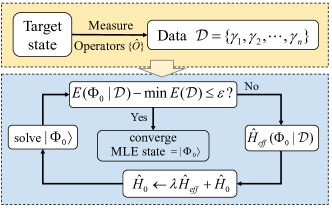
Figure 1: We outline our strategy for the MLE quantum state: given the quantum measurement results, we iteratively update $\hat{H}_{0}$ with $\hat{H}_{eff}$ and solve its ground state $|\Phi_{0}\rangle$, which converges to the MLE state $|\Phi_{gs}\rangle$. The measurement energy $E(\Phi_{0}|\mathcal{D})-\min E(\mathcal{D})$ serves as an indicator of convergence and also reveals whether additional measurements and/or observables are preferable.

Applying such protocol to the measurement energy in Eq. 4, the effective Hamiltonian is:

$$\hat{H}_{eff}=\sum_{\hat{O}}\sum_{\tau}N_{\hat{O}}\alpha_{\tau}\hat{P}_{\tau},\;\alpha_{\tau}=-\frac{f_{\tau}}{\langle\Phi_{gs}|\hat{P}_{\tau}|\Phi_{gs}\rangle},$$ (8)

$N_{\hat{O}}=1$ for single shots. Note that different observables may contribute to the same projection operator. Eq. 8 is one of the main conclusions of this letter: given the quantum measurements, the self-consistent ground state $|\Phi_{gs}\rangle$ of Eq. 8 is our MLE quantum state.

However, as the iteration state approaches the target state, every $\langle\hat{P}_{\tau}\rangle\rightarrow f_{\tau}$, resulting a diminishing $\hat{H}_{eff}$ and unstable eigenstates. Inspired by supervised machine learning [53, 54, 55, 56], we introduce an iteration Hamiltonian $\hat{H}_{0}$, which is initiated randomly and updated as $\hat{H}_{0}\rightarrow\hat{H}_{0}+\lambda\hat{H}_{eff}$, where $\lambda$ is the step size. The ground state $|\Phi_{0}\rangle$ of $\hat{H}_{0}$ moves closer and converges to the MLE state upon updates, while $\hat{H}_{eff}$’s noises average out over the iterations. We summarize the strategy in Fig. 1, and provide further details, rigorous proof, and generalizations to mixed states in Ref. [57, 42].

To see how $\hat{H}_{eff}$ performs as an optimizing gradient for $\hat{H}_{0}$, let’s consider a toy model with a single qubit $|\Phi_{t}(\theta,\varphi)\rangle=\cos(\theta/2)|\hat{z},+\rangle+\sin(\theta/2)e^{i\varphi}|\hat{z},-\rangle$ as the target state. Among various measurements, let us focus on the $\hat{S}_{z}=\sigma^{z}/2$ measurements whose outcomes approach:

$$\lim_{N_{\hat{O}}\to\infty}N_{\pm}=N_{\hat{O}}\langle\Phi_{t}|\hat{P}_{\pm}|\Phi_{t}\rangle=N_{\hat{O}}\frac{(1\pm\cos\theta)}{2},$$ (9)

where $\hat{P}_{\pm}=(1\pm\sigma^{z})/2$ are the projection operators onto the $\sigma^{z}=\pm 1$ eigenspaces, respectively. Correspondingly, given an iteration state $|\Phi_{0}(\theta^{\prime},\varphi^{\prime})\rangle$, these $S_{z}$ measurements contributes to the next $\hat{H}_{eff}$ as follows:

$$N_{\hat{O}}(\alpha_{+}\hat{P}_{+}+\alpha_{-}\hat{P}_{-})=-N_{\hat{O}}\frac{\cos\theta-\cos\theta^{\prime}}{1-\cos^{2}\theta^{\prime}}\sigma^{z}+const.$$ (10)

whose $\sigma^{z}$ coefficient is negative (positive) when $\theta^{\prime}>\theta$ ($\theta^{\prime}<\theta$), opting for a smaller (larger) $\theta^{\prime}$ at the next iteration, and so on till convergence at $\theta$. As $\hat{S}_{z}$ measurements provide no information on $\varphi$, $\varphi^{\prime}$ remains its initial value. Measurements of $\hat{S}_{\bm{n}\neq z}$ contribute additional terms to $\hat{H}_{eff}$ and a more comprehensive optimization of $\hat{H}_{0}$ and $|\Phi_{0}(\theta^{\prime},\varphi^{\prime})\rangle$.

Unlike previous tomography that faces costly direct parameterization of quantum states and challenging non-convex optimization, we encode $|\Phi_{0}\rangle$ intrinsically via $\hat{H}_{0}$, which holds several advantages: our strategy guarantees efficient descent and convergence [42], and also takes advantage of various established quantum many-body ansatzes, such as Lanczos, density-matrix renormalization group [58, 59], and quantum Monte Carlo methods [60, 61], neural network states [43], or quantum simulators [62, 63, 64]. Essentially, the ansatz choice relies on a-priori knowledge, such as symmetries and localities, which allows us to conduct more relevant and efficient searches in Hilbert space sub-manifolds.

It is high time we discussed the choices of observables $\hat{O}$. If the a-priori knowledge about the target state is sufficient, we may choose the most physically relevant measurements, usually lower-order and/or local operators; otherwise, such observables still make a good starting point for tentative studies. In reality, we are often limited by experiments and data availability as well. Fortunately, our strategy can still locate the MLE state even under such circumstances and also tell whether the information is inadequate , upon which one may decide to resort to additional operators or experiments. We illustrate such a procedure on Haar random quantum states without any a-priori knowledge in Ref. [57].

Example: random long-range fermion model —Let’s consider the ground state of the following Hamiltonian:

$$\hat{H}=-\sum_{ij}t_{ij}(c^{\dagger}_{i}c_{j}+c^{\dagger}_{j}c_{i})-\sum_{i}\mu_{i}c^{\dagger}_{i}c_{i},$$ (11)

where $1\leq i,j\leq L$. We apply random $t_{ij}\in[0,1]$ between arbitrary sites and $\mu_{i}\in[-0.5,0.5]$ to deny the system symmetries and locality. Still, our strategy can derive the target states, placed in a black box and tangible only via quantum measurements, even on relatively large systems. Two-point correlators are key to a fermion direct-product state, whose other properties are obtainable via Wick’s theorem, thus we choose the observables $\hat{O}_{i}=c^{\dagger}_{i}c_{i}$ and $\hat{O}^{\prime}_{ij}=(c^{\dagger}_{i}+c^{\dagger}_{j})(c_{i}+c_{j})/2$, each with two eigenvalues , making $\hat{P}_{\tau}$ and $\hat{H}_{eff}$ fermion-bilinear and the subsequent procedure straightforward.

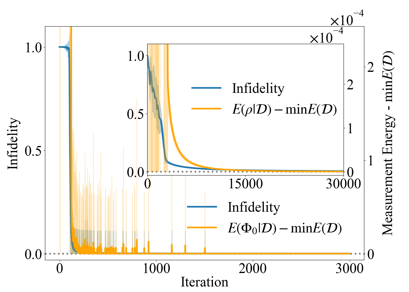
Figure 2: Following our strategy, the iteration state quickly converges to the target quantum state, and the average measurement energy converges to its lower bound. The infidelity for pure state and mixed state (shown in the inset) reaches $\sim 6\times 10^{-4}$ and $\sim 5\times 10^{-3}$, respectively. The shade is based upon 100 trials on different target states - the ground states and Gibbs states of random long-range fermion models with system size $L=100$.

For simplicity, we measure each observable $\hat{O}=\sum_{\tau}\alpha_{\tau}\hat{P}_{\tau}$ on the target quantum state an equal number $N_{\hat{O}}\rightarrow\infty$ of times to suppress fluctuations. Putting these results on $L=100$ systems into the iterative process in Eq. 8, we obtain the results in Fig. 2. We observe a quick convergence of the iteration state $|\Phi_{0}\rangle$ towards the target state, its average measurement energy $E(|\Phi_{0}\rangle)$ towards lower bound . Our strategy also works for data laden with quantum fluctuations due to finite numbers of quantum measurements $N_{\hat{O}}$ and the numerical studies reveal that $N_{\hat{O}}$ necessary for a certain fidelity level scales polynomially to the system size [57].

We also extend applications to mixed states: $\rho_{0}\propto e^{-H_{0}}$ as the quantum state and $\mbox{tr}(\hat{\rho_{0}}\hat{P}_{\tau})$ as the expectation value in Eq. 8. Based on $N_{\hat{O}}\rightarrow\infty$ measurements of $\hat{O}_{i}$ and $\hat{O}^{\prime}_{ij}$ observables for target Gibbs states $\rho_{tar}=e^{-\beta\hat{H}}/\mbox{tr}(e^{-\beta\hat{H}})$ on $\hat{H}$ in Eq. 11 with $L=100$ sites, we observe a quick and unambiguous convergence of the iteration $\rho_{0}$ towards their target (Fig. 2 inset). Further details, examples, and proof for mixed states are in [57, 42].

Example: strongly-correlated Kitaev QSL state—Let’s consider the nearest-neighbor spin Hamiltonian on the honeycomb lattice:

$$\hat{H}=\sum_{\langle ij\rangle\in\alpha\beta(\gamma)}\left[J_{ij}\vec{S}_{i}\cdot\vec{S}_{j}+K_{ij}S_{i}^{\gamma}S_{j}^{\gamma}+\Gamma_{ij}\left(S_{i}^{\alpha}S_{j}^{\beta}+S_{i}^{\beta}S_{j}^{\alpha}\right)\right],$$ (12)

which potentially describes the Kitaev physics in the $A_{2}IrO_{3}$-family iridates [68] and Kitaev material $RuCl_{3}$ [20]. $K_{ij}$, $J_{ij}$, and $\Gamma_{ij}$ are the amplitudes of the Kitaev interaction, isotropic Heisenberg interaction, and the symmetric off-diagonal interactions on bond $\langle ij\rangle$, respectively. Depending on the bond dimension, each bond is labeled by $\alpha\beta(\gamma)$, where $\gamma=x,y,z$ is the spin direction in the Kitaev term, and $\alpha,\beta$ are the two orthogonal spin directions in the $\Gamma_{ij}$ term. The pristine Kitaev model ($J_{ij}=\Gamma_{ij}=0$) is analytically solvable [18, 57]. We take the ground state of $\hat{H}$ with a dominant Kitaev term on a $3\times 3$ system with periodic boundary condition, illustrated in the inset of Fig. 3(b), as our target quantum state. The resulting QSL states are notorious for their lack of smoking-gun signatures. Instead, we probe the target quantum states with seemingly trivial quantum measurements. As we will see, these measurements still provide insightful information, and our strategy leads to the target states and, in turn, their abstract natures, including QSL phase [7, 8, 9] and quantum entanglements [2, 3, 4, 5, 6].

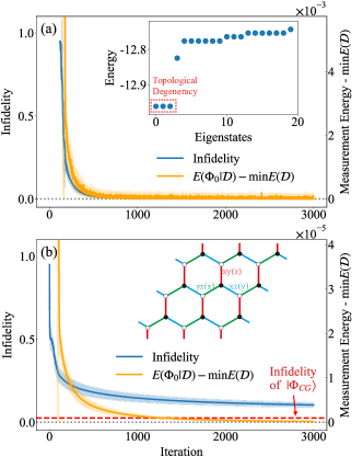
Figure 3: (a) We apply our strategy to the quantum-measurement outcomes of $\sigma_{i}^{\lambda}\sigma_{j}^{\lambda}$, $\lambda=x,y,z$, on one of the ground states of Eq. 12 with $K_{ij}=-1$, $J_{ij}=0.1$, and $\Gamma_{ij}=0$ (spectrum in the inset), the measurement energy $E(\Phi_{0}|\mathcal{D})$ quickly saturates the lower bound, while the iteration states $|\Phi_{0}\rangle$ converge to the target state with infidelity $\sim 10^{-3}$. (b) With the same measurements on the ground states for $K_{ij}=1$, $J_{ij}=0.1$, and $\Gamma_{ij}\in[0,0.1]$, the measurement energy $E(\Phi_{0}|\mathcal{D})$ still quickly saturates the lower bound, while the MLE states $|\Phi_{gs;trial}\rangle$ show slight infidelity $\sim 0.1$ with the target state and differ between trials with average overlap $\sim 0.83$. The red dashed line shows the state $\Phi_{CG}$ averaged over multiple trials [57], which offers an improved approximation with infidelity $\sim 0.03$. The shades are based on multiple trials with different initializations. The inset in (b) is a sketch of the Kitaev model on a $3\times 3$ honeycomb lattice.

To begin with, we set $K_{ij}=-1$, $J_{ij}=0.1$. Given the $C_{3}$ rotation symmetry, there are three degenerate ground states, shown in the inset of Fig. 3(a). These ground states are topologically degenerate with no quasiparticles [57, 29, 18, 69]. The ground states of local Hamiltonians follow the Area law, allowing us to limit to $k$-local, starting from 2-local operators. Here, we first consider quantum measurements on simple observables $\sigma_{i}^{\lambda}\sigma_{j}^{\lambda}$ of each $\langle ij\rangle$ bond on one of the ground states, $\lambda=x,y,z$. Similar quantum measurements are potentially available to QSL models in Rydberg-atom systems [70, 71, 72], or via electron-spin-resonance scanning tunneling microscopy experiments [73, 74], etc. In the large $N_{\hat{O}}\rightarrow\infty$ limit, we obtain $N_{\pm}(ij,\lambda)=N_{\hat{O}}\times\langle\hat{P}_{\pm}(ij,\lambda)\rangle$ counts of $\pm 1$ outcomes, $\hat{P}_{\pm}(ij,\lambda)=(1\pm\sigma_{i}^{\lambda}\sigma_{j}^{\lambda})/2$, respectively. Putting these results into the iterations in Eq. 8, $|\Phi_{0}\rangle$ successfully converges to the target ground-state manifold, see Fig. 3(a). Interestingly, starting from a single ground state, we possess the entire topologically degenerate manifold with high fidelity [57], with which we can achieve fundamental properties such as quasiparticle statistics [7, 8, 9]. On the one hand, these states share identical local properties thus equal qualifications for the MLE states; on the other hand, their simultaneous presence implies that $\hat{H}_{0}$ inherits topological information already present in the target state.

Another interesting scenario is when the observables involved are insufficient to locate the target state fully, as multiple states saturate the measurement energy to the lower bound. For example, we consider the ground state of $K_{ij}=1$, $J_{ij}=0.1$, and random $\Gamma_{ij}\in[0,0.1]$ on each bond. The system possesses a unique ground state without topological degeneracy on a $3\times 3$ system [57]. We keep our observables $\sigma_{i}^{\lambda}\sigma_{j}^{\lambda},\lambda=x,y,z$ and a large number $N_{\hat{O}}\rightarrow\infty$ of quantum measurements as before, whose results on 10 independent trials are summarized in Fig. 3(b). While all trials converge fully and leave little measurement-energy residue, the obtained MLE states $|\Phi_{gs;trial}\rangle$ differ from trial to trial, with an average overlap $\sim 0.83$ in between. We cannot further distinguish these states, which satisfy the quantum measurements equally, until additional observables for further information. Also, we may seek common ground $|\Phi_{CG}\rangle$ between $|\Phi_{gs;trial}\rangle$ as a contingency plan in case of limited ambiguity; see the red dashed line in Fig. 3(b) and details in Ref. [57].

Finally, we consider an unprecedented scenario to showcase the adaptability of our strategy: the observables on nearest-neighbor bonds are $\sigma_{i}^{\hat{n}}\sigma_{j}^{\hat{n}}$ for random $\hat{n}$ directions and measured once each. Such single-shot results, a list of $\pm 1$ outcomes, are plagued with ultimate fluctuations and hard to make use of; nevertheless, our strategy can capitalize on their intrinsic information and unravel the underlying target state. To further increase the challenge, we pick disordered non-Abelian topologically ordered states by setting $K_{ij}=-1$ and random $J_{ij}\in[0,0.1]$, $\Gamma_{ij}\in[0,0.3]$ on each bond for our target quantum many-body states, whose topological properties are analyzed in detail in Ref. [57]. We summarize the demonstration in Fig. 4: the more single shots, the more information at disposal, and the higher the fidelity of the MLE states $|\Phi_{gs}\rangle$; based on a single state, we also obtain the degenerate manifold, even low-lying excited states [57], with high fidelity . We emphasize that although our setup resembles the shadow tomography [76], it neither satisfies nor requires the shadow’s randomness prerequisite. Indeed, our strategy is generally applicable and does not rely on any scheme of measurements.

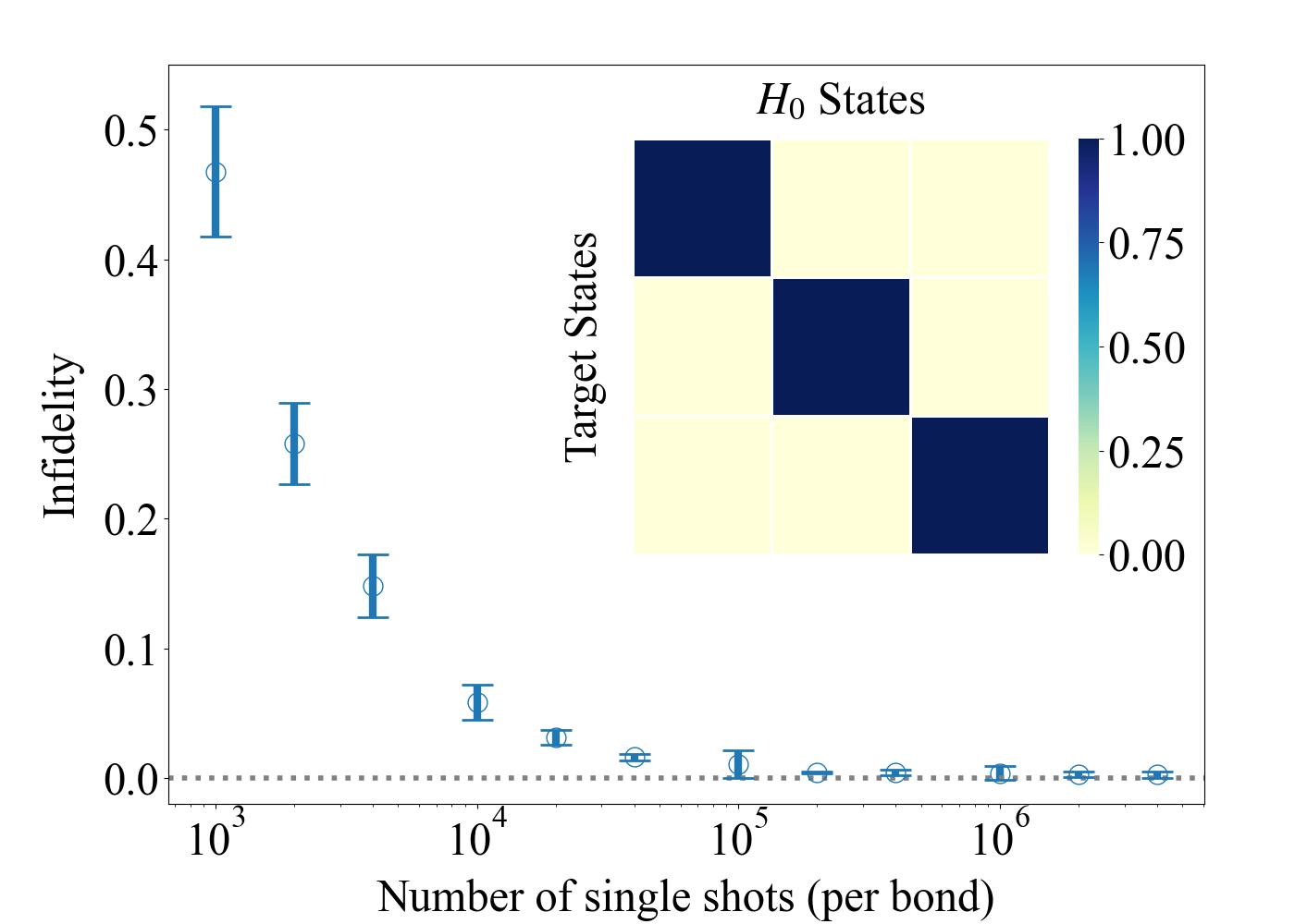
Figure 4: Single-shot quantum measurements $\sigma_{i}^{\hat{n}}\sigma_{j}^{\hat{n}}$ for random $\hat{n}$ directions yield a list of fluctuation-laden $\pm 1$. Based upon such single-shot outcomes from non-Abelian topologically ordered ground states with $K_{ij}=-1$, $J_{ij}\in[0,0.1]$, $\Gamma_{ij}\in[0,0.03]$ in the Kitaev model in Eq. 12, our strategy allows the MLE states to converge asymptotically well to the target states within 1500 iterations as the number of single shots increases. The error bars are based on ten different trials. The inset demonstrates the fidelity between the lowest three eigenstates of the iteration $\hat{H}_{0}$ at convergence and the topological degenerate states of the target system.

Discussions —Considering the exponentially large Hilbert space of a quantum many-body system, we have offered a quantum strategy to interpret quantum measurements in a general and precise way. With full information and reliable convergence, our approach yields state-of-art performance, as demonstrated by several previously-intractable examples above and even for a generic quantum many-body state (in the supplemental materials [57]). We note that the additive form of the measurement energy in Eq. 3 means that every single-shot quantum measurement counts. On the other hand, for cases where the measurement outcomes $\mathcal{D}$ are not directly obtainable, we can reverse engineer values of $f_{\tau}$ from the expectation values $\langle\hat{O}\rangle$, $\langle\hat{O}^{2}\rangle$, $\cdots$ [36], and $N_{\hat{O}}$ as a confidence measure. Our strategy also paves the way for Hamiltonian reconstruction [42, 77, 78]. Generalizations on quantum measurements connecting ground state and excited states, e.g., inelastic spectroscopy experiments, remain an open question for future research.

Acknowledgement: We acknowledge helpful discussions with Zhen-Duo Wang, Tian-Lun Zhao, Pei-Lin Zheng, Hao-Yan Chen, and Yuan Wan. We also acknowledge support from the National Key R&D Program of China (No.2021YFA1401900) and the National Science Foundation of China (No.12174008 & No.92270102). The calculations of this work are supported by HPC facilities at Peking University.

References

- Quintanilla and Hooley [2009] J. Quintanilla and C. Hooley, The strong-correlations puzzle, Physics World 22, 32 (2009).
- Kitaev and Preskill [2006] A. Kitaev and J. Preskill, Topological Entanglement Entropy, Phys. Rev. Lett. 96, 110404 (2006).
- Levin and Wen [2006] M. Levin and X.-G. Wen, Detecting Topological Order in a Ground State Wave Function, Phys. Rev. Lett. 96, 110405 (2006).
- Chen et al. [2010] X. Chen, Z.-C. Gu, and X.-G. Wen, Local unitary transformation, long-range quantum entanglement, wave function renormalization, and topological order, Phys. Rev. B 82, 155138 (2010).
- Zhang et al. [2011a] Y. Zhang, T. Grover, and A. Vishwanath, Topological entanglement entropy of spin liquids and lattice laughlin states, Phys. Rev. B 84, 075128 (2011a).
- Zhang et al. [2011b] Y. Zhang, T. Grover, and A. Vishwanath, Entanglement entropy of critical spin liquids, Phys. Rev. Lett. 107, 067202 (2011b).
- Zhang et al. [2012] Y. Zhang, T. Grover, A. Turner, M. Oshikawa, and A. Vishwanath, Quasiparticle statistics and braiding from ground-state entanglement, Phys. Rev. B 85, 235151 (2012).
- Grover et al. [2013] T. Grover, Y. Zhang, and A. Vishwanath, Entanglement entropy as a portal to the physics of quantum spin liquids, New Journal of Physics 15, 025002 (2013).
- Zhang et al. [2015] Y. Zhang, T. Grover, and A. Vishwanath, General procedure for determining braiding and statistics of anyons using entanglement interferometry, Phys. Rev. B 91, 035127 (2015).
- Haldane [1988] F. D. M. Haldane, Model for a quantum hall effect without landau levels: Condensed-matter realization of the ”parity anomaly”, Phys. Rev. Lett. 61, 2015 (1988).
- Laughlin [1983] R. B. Laughlin, Anomalous quantum hall effect: An incompressible quantum fluid with fractionally charged excitations, Phys. Rev. Lett. 50, 1395 (1983).
- Kane and Mele [2005] C. L. Kane and E. J. Mele, topological order and the quantum spin hall effect, Phys. Rev. Lett. 95, 146802 (2005).
- Hasan and Kane [2010] M. Z. Hasan and C. L. Kane, Colloquium : Topological insulators, Rev. Mod. Phys. 82, 3045 (2010).
- Nielsen and Ninomiya [1983] H. Nielsen and M. Ninomiya, The adler-bell-jackiw anomaly and weyl fermions in a crystal, Physics Letters B 130, 389 (1983).
- Yuan et al. [2020] X. Yuan, C. Zhang, Y. Zhang, Z. Yan, T. Lyu, M. Zhang, Z. Li, C. Song, M. Zhao, P. Leng, M. Ozerov, X. Chen, N. Wang, Y. Shi, H. Yan, and F. Xiu, The discovery of dynamic chiral anomaly in a weyl semimetal nbas, Nature Communications 11, 1259 (2020).
- Keimer and Moore [2017] B. Keimer and J. E. Moore, The physics of quantum materials, Nature Physics 13, 1045 (2017).
- Kitaev [2003] A. Kitaev, Fault-tolerant quantum computation by anyons, Annals of Physics 303, 2 (2003).
- Kitaev [2006] A. Kitaev, Anyons in an exactly solved model and beyond, Annals of Physics 321, 2 (2006).
- Yan et al. [2011] S. Yan, D. A. Huse, and S. R. White, Spin-liquid ground state of the s = 1/2 kagome heisenberg antiferromagnet, Science 332, 1173 (2011).
- Banerjee et al. [2016] A. Banerjee, C. A. Bridges, J.-Q. Yan, A. A. Aczel, L. Li, M. B. Stone, G. E. Granroth, M. D. Lumsden, Y. Yiu, J. Knolle, S. Bhattacharjee, D. L. Kovrizhin, R. Moessner, D. A. Tennant, D. G. Mandrus, and S. E. Nagler, Proximate kitaev quantum spin liquid behaviour in a honeycomb magnet, Nature Materials 15, 733 (2016).
- Bednorz and Müller [1986] J. G. Bednorz and K. A. Müller, Possible hight c superconductivity in the ba- la- cu- o system, Zeitschrift für Physik B Condensed Matter 64, 189 (1986).
- Kamihara et al. [2006] Y. Kamihara, H. Hiramatsu, M. Hirano, R. Kawamura, H. Yanagi, T. Kamiya, and H. Hosono, Iron-based layered superconductor: Laofep, Journal of the American Chemical Society 128, 10012 (2006).
- Kamihara et al. [2008] Y. Kamihara, T. Watanabe, M. Hirano, and H. Hosono, Iron-based layered superconductor la [o1-x f x] feas (x= 0.05- 0.12) with t c= 26 k, Journal of the American Chemical Society 130, 3296 (2008).
- Cao et al. [2018] Y. Cao, V. Fatemi, S. Fang, K. Watanabe, T. Taniguchi, E. Kaxiras, and P. Jarillo-Herrero, Unconventional superconductivity in magic-angle graphene superlattices, Nature 556, 43 (2018).
- Klitzing et al. [1980] K. v. Klitzing, G. Dorda, and M. Pepper, New method for high-accuracy determination of the fine-structure constant based on quantized hall resistance, Phys. Rev. Lett. 45, 494 (1980).
- Tsui et al. [1982] D. C. Tsui, H. L. Stormer, and A. C. Gossard, Two-dimensional magnetotransport in the extreme quantum limit, Phys. Rev. Lett. 48, 1559 (1982).
- Haldane [1983] F. D. M. Haldane, Nonlinear field theory of large-spin heisenberg antiferromagnets: Semiclassically quantized solitons of the one-dimensional easy-axis néel state, Phys. Rev. Lett. 50, 1153 (1983).
- von Klitzing [1986] K. von Klitzing, The quantized hall effect, Rev. Mod. Phys. 58, 519 (1986).
- Wen and Niu [1990] X. G. Wen and Q. Niu, Ground-state degeneracy of the fractional quantum hall states in the presence of a random potential and on high-genus riemann surfaces, Phys. Rev. B 41, 9377 (1990).
- Haldane [2004] F. D. M. Haldane, Berry curvature on the fermi surface: Anomalous hall effect as a topological fermi-liquid property, Phys. Rev. Lett. 93, 206602 (2004).
- Bernevig et al. [2006] B. A. Bernevig, T. L. Hughes, and S.-C. Zhang, Quantum spin hall effect and topological phase transition in hgte quantum wells, Science 314, 1757 (2006).
- Fu et al. [2007] L. Fu, C. L. Kane, and E. J. Mele, Topological insulators in three dimensions, Phys. Rev. Lett. 98, 106803 (2007).
- Chen et al. [2012] X. Chen, Z.-C. Gu, Z.-X. Liu, and X.-G. Wen, Symmetry-Protected Topological Orders in Interacting Bosonic Systems, Science 338, 1604 (2012).
- Fradkin et al. [2015] E. Fradkin, S. A. Kivelson, and J. M. Tranquada, Colloquium, Rev. Mod. Phys. 87, 457 (2015).
- Proust and Taillefer [2019] C. Proust and L. Taillefer, The remarkable underlying ground states of cuprate superconductors, Annual Review of Condensed Matter Physics 10, 409 (2019).
- Sakurai and Napolitano [2011] J. J. Sakurai and J. Napolitano, Modern quantum mechanics; 2nd ed. (Addison-Wesley, San Francisco, CA, 2011).
- Han et al. [2012] T.-H. Han, J. S. Helton, S. Chu, D. G. Nocera, J. A. Rodriguez-Rivera, C. Broholm, and Y. S. Lee, Fractionalized excitations in the spin-liquid state of a kagome-lattice antiferromagnet, Nature 492, 406 (2012).
- Lvovsky and Raymer [2009] A. I. Lvovsky and M. G. Raymer, Continuous-variable optical quantum-state tomography, Rev. Mod. Phys. 81, 299 (2009).
- Torlai et al. [2018] G. Torlai, G. Mazzola, J. Carrasquilla, M. Troyer, R. Melko, and G. Carleo, Neural-network quantum state tomography, Nature Physics 14, 447 (2018).
- Carrasquilla et al. [2019] J. Carrasquilla, G. Torlai, R. G. Melko, and L. Aolita, Reconstructing quantum states with generative models, Nat. Mach. Intell. 1, 155 (2019).
- Huang et al. [2020a] H.-Y. Huang, R. Kueng, and J. Preskill, Predicting many properties of a quantum system from very few measurements, Nature Physics 16, 1050 (2020a).
- Zhao et al. [2022] T.-L. Zhao, S.-X. Hu, and Y. Zhang, Supervised hamiltonian learning via efficient and robust quantum descent (2022), arXiv:2212.13718 .
- Carleo and Troyer [2017] G. Carleo and M. Troyer, Solving the quantum many-body problem with artificial neural networks, Science 355, 602 (2017).
- Huszár and Houlsby [2012] F. Huszár and N. M. Houlsby, Adaptive bayesian quantum tomography, Physical Review A 85, 052120 (2012).
- Note [1] Unlike the expectation value of a linear operator, the measurement energy is explicitly nonlinear due to the function. Therefore, the probability distribution of a quantum state with measurement outcomes offers realizations of exotic nonlinear-operator Hamiltonian.
- Hradil et al. [2004] Z. Hradil, J. Řeháček, J. Fiurášek, and M. Ježek, 3 maximum-likelihood methodsin quantum mechanics, in Quantum state estimation (Springer, 2004) pp. 59–112.
- Altepeter et al. [2005] J. Altepeter, E. Jeffrey, and P. Kwiat, Photonic state tomography (Academic Press, 2005) pp. 105–159.
- Hradil [1997] Z. Hradil, Quantum-state estimation, Phys. Rev. A 55, R1561 (1997).
- Řeháček et al. [2001] J. Řeháček, Z. Hradil, and M. Ježek, Iterative algorithm for reconstruction of entangled states, Phys. Rev. A 63, 040303 (2001).
- James et al. [2001] D. F. V. James, P. G. Kwiat, W. J. Munro, and A. G. White, Measurement of qubits, Phys. Rev. A 64, 052312 (2001).
- Shang et al. [2017] J. Shang, Z. Zhang, and H. K. Ng, Superfast maximum-likelihood reconstruction for quantum tomography, Phys. Rev. A 95, 062336 (2017).
- Řeháček et al. [2007] J. Řeháček, Z. c. v. Hradil, E. Knill, and A. I. Lvovsky, Diluted maximum-likelihood algorithm for quantum tomography, Phys. Rev. A 75, 042108 (2007).
- Michael Nielsen [2013] Michael Nielsen, Neural Networks and Deep Learning (Free Online Book, 2013).
- Carrasquilla and Melko [2017] J. Carrasquilla and R. G. Melko, Machine learning phases of matter, Nature Physics 13, 431 (2017).
- Zhang and Kim [2017] Y. Zhang and E.-A. Kim, Quantum Loop Topography for Machine Learning, Phys. Rev. Lett. 118, 216401 (2017).
- Zhang et al. [2019] Y. Zhang, A. Mesaros, K. Fujita, S. Edkins, M. Hamidian, K. Ch’ng, H. Eisaki, S. Uchida, J. S. Davis, E. Khatami, et al., Machine learning in electronic-quantum-matter imaging experiments, Nature 570, 484 (2019).
- [57] See examples and details on hyper-parameters, finite number of measurements, interacting fermion models, topological degeneracy of the Kitaev model, contingency plan for insufficiency observables, generalization to mixed states and Haar random states without a-priori knowledge in Supplemental Materials, which also include Ref. 79, 80, 81, 82, 83, 84, 85, 86, 87.
- Fannes et al. [1992] M. Fannes, B. Nachtergaele, and R. F. Werner, Finitely correlated states on quantum spin chains, Communications in Mathematical Physics 144, 443 (1992).
- Schollwöck [2005] U. Schollwöck, The density-matrix renormalization group, Rev. Mod. Phys. 77, 259 (2005).
- Foulkes et al. [2001] W. M. C. Foulkes, L. Mitas, R. J. Needs, and G. Rajagopal, Quantum monte carlo simulations of solids, Rev. Mod. Phys. 73, 33 (2001).
- Troyer and Wiese [2005] M. Troyer and U.-J. Wiese, Computational complexity and fundamental limitations to fermionic quantum monte carlo simulations, Phys. Rev. Lett. 94, 170201 (2005).
- Farhi et al. [2014] E. Farhi, J. Goldstone, and S. Gutmann, A quantum approximate optimization algorithm (2014), arXiv:1411.4028 [quant-ph] .
- Zhou et al. [2020] L. Zhou, S.-T. Wang, S. Choi, H. Pichler, and M. D. Lukin, Quantum approximate optimization algorithm: Performance, mechanism, and implementation on near-term devices, Phys. Rev. X 10, 021067 (2020).
- Vikstål et al. [2020] P. Vikstål, M. Grönkvist, M. Svensson, M. Andersson, G. Johansson, and G. Ferrini, Applying the quantum approximate optimization algorithm to the tail-assignment problem, Phys. Rev. Applied 14, 034009 (2020).
- Note [2] A lack of observables may lead to misleading MLE states, which we can identify with signatures in measurement energy: it may constrain the search space leading to a sub-optimal MLE state as the measurement energy converges above its lower bound, or end up with different MLE states simultaneously consistent with the measurement outcomes.
- Note [3] An observable with more eigenvalues acts as a double-edged sword: they may incur cost in post-processing due to more complex , but the distribution also offer more information than the average in a similar spirit to shot-noise studies [88, 89]. We can make an observable simpler to handle by binning together some outcomes and giving up some information, but not vice versa.
- Note [4] The spikes in the figure are mainly due to the inconsistent particle number the iteration state receives over the slight modifications. Better convergence largely suppresses such phenomena in later iterations.
- Rau et al. [2014] J. G. Rau, E. K.-H. Lee, and H.-Y. Kee, Generic spin model for the honeycomb iridates beyond the kitaev limit, Phys. Rev. Lett. 112, 077204 (2014).
- Hastings and Wen [2005] M. B. Hastings and X.-G. Wen, Quasiadiabatic continuation of quantum states: The stability of topological ground-state degeneracy and emergent gauge invariance, Phys. Rev. B 72, 045141 (2005).
- Verresen et al. [2021] R. Verresen, M. D. Lukin, and A. Vishwanath, Prediction of toric code topological order from rydberg blockade, Phys. Rev. X 11, 031005 (2021).
- Semeghini et al. [2021] G. Semeghini, H. Levine, A. Keesling, S. Ebadi, T. T. Wang, D. Bluvstein, R. Verresen, H. Pichler, M. Kalinowski, R. Samajdar, A. Omran, S. Sachdev, A. Vishwanath, M. Greiner, V. Vuletić, and M. D. Lukin, Probing topological spin liquids on a programmable quantum simulator, Science 374, 1242 (2021).
- Samajdar et al. [2021] R. Samajdar, W. W. Ho, H. Pichler, M. D. Lukin, and S. Sachdev, Quantum phases of rydberg atoms on a kagome lattice, Proceedings of the National Academy of Sciences 118, e2015785118 (2021), https://www.pnas.org/doi/pdf/10.1073/pnas.2015785118 .
- Balatsky et al. [2012] A. V. Balatsky, M. Nishijima, and Y. Manassen, Electron spin resonance-scanning tunneling microscopy, Advances in Physics 61, 117 (2012).
- Ternes [2015] M. Ternes, Spin excitations and correlations in scanning tunneling spectroscopy, New Journal of Physics 17, 063016 (2015).
- Note [5] Note that a measurement-energy lower bound is no longer available for such single-shot measurements.
- Huang et al. [2020b] H.-Y. Huang, R. Kueng, and J. Preskill, Predicting many properties of a quantum system from very few measurements, Nature Physics 16, 1050 (2020b).
- Qi and Ranard [2019] X.-L. Qi and D. Ranard, Determining a local hamiltonian from a single eigenstate, Quantum 3, 159 (2019).
- Turkeshi et al. [2019] X. Turkeshi, T. Mendes-Santos, G. Giudici, and M. Dalmonte, Entanglement-guided search for parent hamiltonians, Phys. Rev. Lett. 122, 150606 (2019).
- Chaloupka et al. [2010] J. c. v. Chaloupka, G. Jackeli, and G. Khaliullin, Kitaev-heisenberg model on a honeycomb lattice: Possible exotic phases in iridium oxides , Phys. Rev. Lett. 105, 027204 (2010).
- Mandal and Jayannavar [2020] S. Mandal and A. M. Jayannavar, An introduction to kitaev model-i, arXiv preprint arXiv:2006.11549 (2020).
- Lieb [1994] E. H. Lieb, Flux phase of the half-filled band, Phys. Rev. Lett. 73, 2158 (1994).
- Pedrocchi et al. [2011] F. L. Pedrocchi, S. Chesi, and D. Loss, Physical solutions of the kitaev honeycomb model, Phys. Rev. B 84, 165414 (2011).
- Zschocke and Vojta [2015] F. Zschocke and M. Vojta, Physical states and finite-size effects in kitaev’s honeycomb model: Bond disorder, spin excitations, and nmr line shape, Phys. Rev. B 92, 014403 (2015).
- Zhu et al. [2018] Z. Zhu, I. Kimchi, D. N. Sheng, and L. Fu, Robust non-abelian spin liquid and a possible intermediate phase in the antiferromagnetic kitaev model with magnetic field, Phys. Rev. B 97, 241110 (2018).
- Dawid et al. [2022] A. Dawid, J. Arnold, B. Requena, A. Gresch, M. Płodzień, K. Donatella, K. Nicoli, P. Stornati, R. Koch, M. Büttner, R. Okuła, G. Muñoz-Gil, R. A. Vargas-Hernández, A. Cervera-Lierta, J. Carrasquilla, V. Dunjko, M. Gabrié, P. Huembeli, E. van Nieuwenburg, F. Vicentini, L. Wang, S. J. Wetzel, G. Carleo, E. Greplová, R. Krems, F. Marquardt, M. Tomza, M. Lewenstein, and A. Dauphin, Modern applications of machine learning in quantum sciences (2022).
- Teo et al. [2012] Y. S. Teo, B. Stoklasa, B.-G. Englert, J. Řeháček, and Z. c. v. Hradil, Incomplete quantum state estimation: A comprehensive study, Phys. Rev. A 85, 042317 (2012).
- Biswas et al. [2021] G. Biswas, A. Biswas, and U. Sen, Inhibition of spread of typical bipartite and genuine multiparty entanglement in response to disorder, New Journal of Physics 23, 113042 (2021).
- Zhou et al. [2019] P. Zhou, L. Chen, Y. Liu, I. Sochnikov, A. T. Bollinger, M.-G. Han, Y. Zhu, X. He, I. Bozovic, and D. Natelson, Electron pairing in the pseudogap state revealed by shot noise in copper oxide junctions, Nature 572, 493 (2019).
- Sivre et al. [2019] E. Sivre, H. Duprez, A. Anthore, A. Aassime, F. D. Parmentier, A. Cavanna, A. Ouerghi, U. Gennser, and F. Pierre, Electronic heat flow and thermal shot noise in quantum circuits, Nature Communications 10, 5638 (2019).