Time-assisted energy reconstruction in a highly-granular hadronic calorimeter

Abstract

The software compensation algorithms developed for the CALICE Analog Hadron Calorimeter are extended to incorporate time information on the cell level, and the performance is studied in GEANT4 simulations with a detector model of a highly-granular SiPM-on-tile calorimeter. The addition of nanosecond-level time resolution is found to result in significant improvement of the energy resolution by approximately $3\text{\,}\mathrm{\char 37\relax}4\text{\,}\mathrm{\char 37\relax}$ for local software compensation compared to the software compensation based on local energy density alone, with further improvement possible with better timing resolution. The high correlation of energy density and time variables show that both provide sensitivity to correlated underlying shower features, which limits the potential of timing information when used as a global rather than a local variable.

1 Introduction

Highly-granular electromagnetic and hadronic calorimeters are a crucial part of particle-flow-centred detectors at future $e^{+}e^{-}$ colliders [1, 2, 3]. The Analog Hadron Calorimeter (AHCAL) developed by the CALICE collaboration represents one concept for a highly-granular hadronic calorimeter [4]. It is a sampling calorimeter on plastic scintillator basis read out by Silicon Photomultipliers with cell sizes of $$3$\times$3\text{\,}\mathrm{c}\mathrm{m}^{2}$$.

While the spatial resolution and the separation of showers inside a particle jet play a key role in particle flow detectors [1], the energy resolution of the hadronic calorimeter still adds to the overall detector performance, both via the improvement of the energy measurement of neutral hadrons, and through improved cluster-track matching in particle-flow algorithms (PFA) due to more accurate energy estimates of clusters assigned to charged particles [5]. In longitudinally and transversely segmented non-compensating hadronic calorimeters the energy resolution for hadronic showers can be improved by amplitude or energy-density dependent offline weighting of the measured signals in individual detector cells [6, 7, 8], exploiting the difference in response to electromagnetic and purely hadronic components of the showers. The high granularity of the CALICE calorimeters makes them perfectly suited for such reconstruction techniques, which have been developed under the term software compensation [9] for highly-granular calorimeters. For the AHCAL, an improvement of the hadronic energy resolution of approximately 20% compared to a reconstruction without such techniques was achieved.

Since the large-scale physics prototypes constructed by CALICE in the mid-2000s, the technology of highly-granular calorimeters has evolved, both on the sensor side with improved performance and better device-to-device uniformity, and in the area of front-end electronics, most notably by providing cell-by-cell time measurements. This enables the full five-dimensional reconstruction of particle showers in space, local energy density or amplitude, and time. The large technological prototype (LTP) of the AHCAL [10], a 22 000 channel, 0.5 m³ SiPM-on-tile highly-granular hadronic calorimeter with steel absorbers, which was first operated in beam tests with hadrons in 2018, has the ability to provide hit-time measurements on the cell level with nanosecond precision, as demonstrated in preliminary studies [11]. This capability may allow conclusions about the amount of slow neutrons generated in the shower, since measurements with different absorber materials have shown that delayed components in the signals in hadronic calorimeters are primarily due to the neutron component in the shower. Examples that show this connection of neutron activity and late signals are measurements in steel and uranium calorimeters [12, 13], in a scintillating fiber calorimeter with lead absorber [14] and in a copper-based dual readout calorimeter [15]. Shower energy that is absorbed in the generation of neutrons during the spallation processes to overcome the nuclear binding energy is lost for calorimetric purposes. Thus estimating the amount of neutrons in a given shower may result in an improvement of the energy measurement. The extension of the software compensation techniques used for highly-granular calorimeters to include time as an additional dimension is thus of high interest to explore the potential in this area.

In the following, methods are presented for incorporating the timing capabilities of a highly-granular hadronic calorimeter into the energy reconstruction. For this, two different approaches to software compensation, a global and a local one, are presented, extending the techniques developed in [9] to include the time domain in addition to purely energy-based observables. All methods are developed and evaluated on simulated data.

2 Detector geometry and simulated data

The detector geometry used for the simulation is a sampling calorimeter with steel absorber and 60 active layers. The design follows that of the CALICE AHCAL LTP, but with an increased number of layers to reduce the effect of longitudinal energy leakage on the energy reconstruction. The active elements of the calorimeter are $$3\text{\,}$\times$3\text{\,}\mathrm{c}\mathrm{m}^{2}$$ polystyrene-based scintillator tiles with the scintillation light read out by SiPMs housed on electronics boards with integrated front-end ASICs [10]. Each active layer consists of 576 channels, resulting in a transverse size of $$72\text{\,}$\times$72\text{\,}\mathrm{c}\mathrm{m}^{2}$$. The total stainless steel absorber thickness per layer is $17\text{\,}\mathrm{m}\mathrm{m}$, with $16\text{\,}\mathrm{m}\mathrm{m}$ provided by the mechanical absorber structure itself, and $1\text{\,}\mathrm{m}\mathrm{m}$ from the cassettes housing the active elements. The LTP has 38 layers, which is not sufficiently deep to fully contain higher-energy hadronic showers without an additional tail catcher with coarser longitudinal sampling, or an electromagnetic calorimeter upstream of the hadronic calorimeter. To avoid energy-leakage-induced distortions of the energy resolution studies discussed in the present paper, 60 active layers and the corresponding absorbers have been simulated. The simulation was performed using the DD4HEP [16] framework in combination with GEANT4 v10.03 [17]. The QGSP_BERT_HP physics list was used for all GEANT4 simulation samples discussed in this study. Scintillator saturation was implemented using a Birks’ parameter of $k_{B}\,=\,0.07943\,$\text{\,}\mathrm{m}\mathrm{m}\mathrm{M}\mathrm{e}\mathrm{V}^{-1}$$ [18].

The idealized energy depositions generated by GEANT4 are combined per detector cell, assuming a maximum integration time of $2000\text{\,}\mathrm{ns}$, and are transformed into hits in a digitization process that mimics the detector effects. The influence of the SiPMs response on the signal is simulated via discretization into photoelectrons and Poissonian smearing, as well as a simulation of the saturation effects originating from the finite number of pixels in the sensor. The front-end electronics are taken into account via a simulation of shaping effects by combination of energy deposits within 50 ns into a single hit, and the addition of electronics noise, which manifests as additional smearing of the signal amplitude. The energy depositions in units of $\text{\,}\mathrm{keV}$ are converted to the MIP scale by a factor of $477\text{\,}\mathrm{k}\mathrm{eV}\mathrm{/}\text{MIP}$. This factor is calibrated such that a minimum ionizing particle (MIP) (i.e., a muon in the $\text{\,}\mathrm{GeV}$ range) has a most probable energy deposition of $1\text{\,}\text{MIP}$ in a scintillator tile traversed at normal incidence. Detector cells with an energy deposition below $0.5\text{\,}\text{MIP}$ are not considered in the analysis, in line with the threshold typically applied in the analysis of CALICE AHCAL data. For the time measurements a gaussian smearing with a resolution of $1\text{\,}\mathrm{ns}$ is applied to the generator-level time stamp of the hit, which is given by the time of the first energy deposit in the cell.

The CALICE collaboration has observed good agreement between test beam data of its physics prototype and simulated hadronic showers with respect to the hit energy distributions and shower shapes [19]. It was shown by the CALICE T3B Experiment that the time distribution of hadronic showers, as simulated by GEANT4 with the physics list used in the present study, is in good agreement with the simulations using a steel absorber [20].

3 Correlation of energy and time observables

The overall hit time distribution for $40\text{\,}\mathrm{GeV}$ pions is shown in 1(a) on two different time scales. The zero time is calibrated such that a muon hitting a cell would produce a time stamp of $t=0$. Thus, the time of flight of the particles between the layers is already taken into account in the calibration. Time stamps below zero are due to the smearing introduced by the finite time resolution. In 1(a) three different regimes can be identified: The instantaneous part up to about $3\text{\,}\mathrm{ns}$, governed by the time resolution of the detector, an intermediate, exponentially falling, part mainly due to hits caused by neutron elastic scattering, and a late tail dominated by neutron capture events. In the present study, the fraction of energy deposited later than $3\text{\,}\mathrm{ns}$ is adopted as the variable to characterize the timing behaviour of an event. The hits contributing to this fraction are indicated in red in 1(a). In 1(b) the median value of this fraction is shown over the range of beam energies considered. The shaded region visualizes the central $50\text{\,}\mathrm{\char 37\relax}$-interval. The median value is about $3\text{\,}\mathrm{\char 37\relax}$ for most beam energies and slightly higher for lower energies. The monotonic decrease of this value is expected, as the electromagnetic fraction is increasing for higher energies, resulting in a reduction of the influence of the neutron-dominated later parts of the shower.

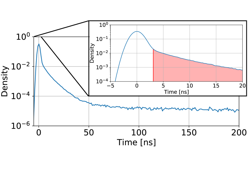
(a)

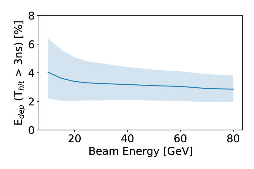
(b)

Figure 1: (a) Hit time distribution for $40\text{\,}\mathrm{GeV}$ pions in the simulated calorimeter on a larger and smaller time scale. For the smaller time scale, the hit times above $3\text{\,}\mathrm{ns}$, which are called late throughout this study, are indicated in red. (b) Median of the fraction of measured late energy deposistions in a shower. The shaded region indicates the $50\text{\,}\mathrm{\char 37\relax}$ quantile.

2(a) shows the 2D-distribution of the fraction of late energy depositions in an event and the relative difference of the reconstructed energy to the beam energy ($\Delta E$) for $40\text{\,}\mathrm{GeV}$ pions. It can be seen that for low values of the fraction of late energy deposits ($E_{\text{dep}}(T_{\text{hit}}>$3\text{\,}\mathrm{ns}$)$) on average the reconstructed energy is too high, while for high fractions of late energy depositions the reconstructed energy tends to be too low. This observation is in line with the interpretation that a large amount of late energy depositions indicates a high hadronic fraction and thus a lower calorimeter response. For comparison in 2(b) $\Delta E$ is shown dependent on $C_{\text{global}}$, an observable that describes the hit energy distribution of an event and which was developed to correct the reconstructed energy within the AHCAL [9] in the global software compensation scheme. This variable is defined as the ratio between the fraction of hits in the calorimeter with energy depositions larger than $5\text{\,}\text{MIP}$ ($C_{\text{thr}}$) and the fraction of hits with energy depositions larger than the average hit energy in this shower ($C_{\text{av}}$):

$$C_{\text{global}}=\frac{C_{\text{thr}}}{C_{\text{av}}}.$$ (3.1)

This variable exhibits a positive correlation with $\Delta E$, which was exploited in [9] to improve the energy resolution of the calorimeter.

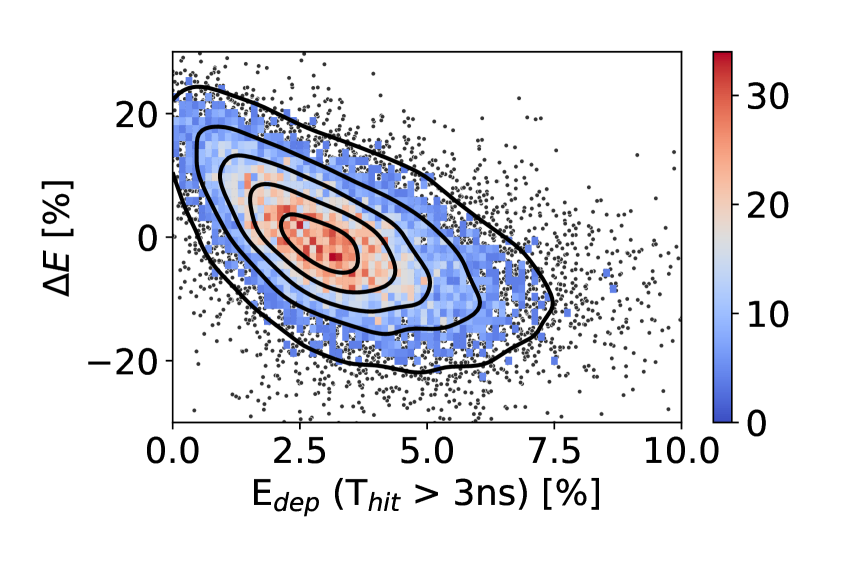
(a)

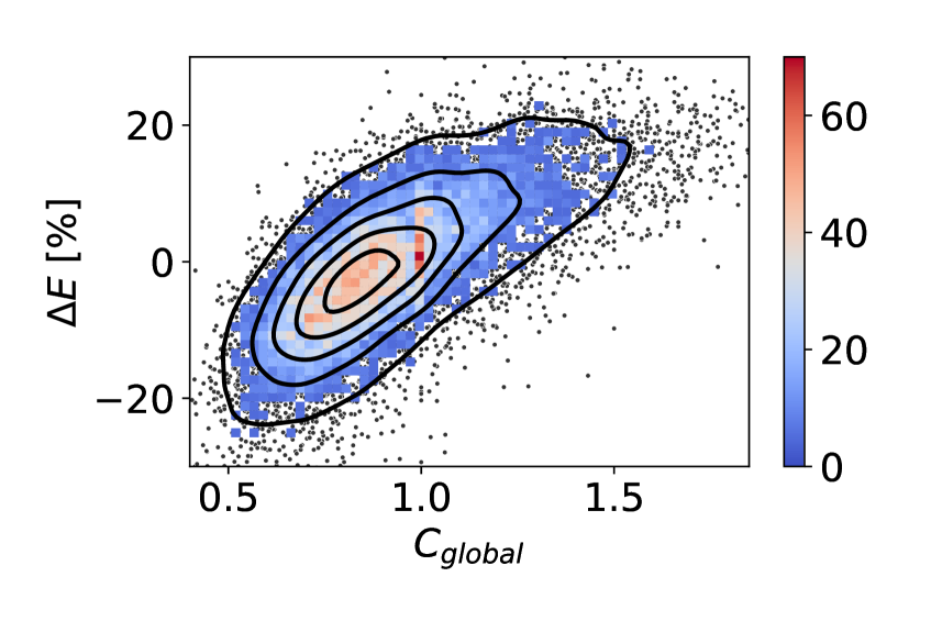
(b)

Figure 2: Correlation of (a) the fraction of late energy deposits and (b) $C_{\text{global}}$ with the ratio of the reconstructed to the true beam energy ($\Delta E$). The amount of entries in the highest density bins holding $90\text{\,}\mathrm{\char 37\relax}$ of the data are indicated by the color scale, while the remaining lower density bins are shown as individual data points (gray). Additionally, contour lines generated by a kernel density estimation are drawn in black.

In Figure 3 the absolute value of the correlation coefficients between the fraction of late energy hits and $C_{\text{global}}$ with $\Delta E$ are shown over the full energy range. Significant correlations of both observables with the reconstructed energy are visible. For $C_{\text{global}}$, however, the correlation is consistently higher than for the time-based observable. For higher energies the correlation coefficients are slightly higher, because of the lower statistical uncertainty resulting from the larger number of hits in these events. The large correlation coefficients observed indicate that both observables can be used to enhance the energy resolution of the AHCAL.

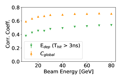
Figure 3: Pearson correlation coefficients of the reconstructed energy ($E_{\text{std}}$, see section 4) with the fraction of late energy deposits (green) and $C_{\text{global}}$ (orange).

In order to study the interplay of the correlation of the late energy depositions and $C_{\text{global}}$ with $\Delta E$, we decompose the $C_{\text{global}}$ variable and look at the correlations with $\Delta E$ separately. The numerator in the definition of $C_{\text{global}}$ is $C_{\text{thr}}$ describing the fraction of the hits in a shower that are of high energy density, thus being sensitive to the electromagnetic part of the shower. The fraction of late energy deposits is sensitive to the amount of neutron interaction in the shower. In 4(a) the data of $30\text{\,}\mathrm{GeV}50\text{\,}\mathrm{GeV}$ pions is binned with respect to both variables, $C_{\text{thr}}$ and $E_{\text{dep}}(T_{\text{hit}}>$3\text{\,}\mathrm{ns}$)$. Additionally the deviation of the reconstructed to the true energy ($\Delta E$) is indicated as the color scale. Areas of lighter color indicate a too high energy reconstruction, while areas of darker color indicate a too low reconstructed energy. The contour lines of the color space are indicated as a yellow dotted line. It can be seen that the contour lines are not horizontal and thus both variables are necessary to explain the variance in $\Delta E$. Both information of the size of the electromagnetic part as well as of the neutron activity are necessary for an optimal explanation of $\Delta E$.

In 4(b) the data is binned with respect to $C_{\text{global}}$ on the $y$-axis. In this case, the contour lines are nearly parallel to the $x$-axis indicating that $C_{\text{global}}$ incorporates information about the electromagnetic part of the shower as well as the neutron activity and thus the timing information only adds marginal value for an improved reconstruction of the energy with respect to the information encoded in $C_{\text{global}}$.

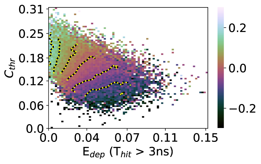
(a)

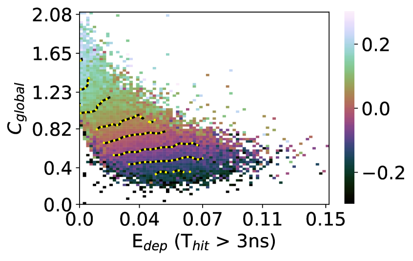
(b)

Figure 4: Mean relative deviation of the reconstructed and true energy for $30\text{\,}\mathrm{GeV}50\text{\,}\mathrm{GeV}$ pions in each bin shown by the color scale. The data is binned with respect to the fraction of late energy deposits ($E_{\text{dep}}(T_{\text{hit}}>$3\text{\,}\mathrm{ns}$)$) and (a) $C_{\text{thr}}$ and (b) $C_{\text{global}}$. The yellow dotted line indicates the smoothed contour lines of the color space.

4 Methods

The standard energy reconstruction method of a hadronic shower $i$ is the sum of all hit energies $e_{j}$:

$$E_{\text{std},i}=\sum_{j\,\in\,\text{hits}}e_{j,i}.$$ (4.1)

The software compensation methods improve on this simple reconstruction by learning weights to down- or upweight certain parts of the shower. Two different methods are discussed for the time assisted energy reconstruction in the following: A global and a local software compensation technique.

4.1 Global software compensation

The global software compensation technique corrects the energy sum of the standard reconstruction $E_{\text{std}}$ by a global correction factor, which is a function of an observable $\theta$ of the shower. In previous work the aforementioned $C_{\text{global}}$ variable was used as the observable $\theta$ [9]. The correction factor is a second order polynomial of $\theta$, such that the reconstructed energy of event $i$ becomes:

$$E_{\text{reco},i}^{\text{global}}=E_{\text{std},i}\cdot(a+b\,\theta_{i}+c\,\theta_{i}^{2}).$$ (4.2)

The parameters $a$, $b$, and $c$ are determined by an optimization procedure minimizing the following loss function:

$$L=\sum_{i\,\in\,\text{events}}\frac{\left(E_{\text{reco},i}^{\text{global}}-E_{\text{beam},i}\right)^{2}}{E_{\text{beam},i}},$$ (4.3)

where the sum runs over all events in the sample and $E_{\text{beam}}$ is the simulated true beam energy. In order to incorporate the hit time measurements into this approach, it can be extended by using a second observable $\phi$:

$$E_{\text{reco},i}^{\text{global}}=E_{\text{std},i}\cdot(a+b\,\theta_{i}+c\,\phi_{i}+d\,\theta_{i}\phi_{i}),$$ (4.4)

where, in this case, $\phi_{i}$ is the fraction of late energy depositions in a shower. In order to limit the overall number of parameters the quadratic terms are omitted in this approach, but a correlation term $\theta_{i}\phi_{i}$ is added. The additional improvement from the quadratic terms on the energy reconstruction is much smaller compared to that achieved with the already considered terms.

As the parameters $a$ to $d$ are expected to change with the beam energy they are determined for every training beam energy separately. The resulting parameters are then fitted with a quadratic function such that:

$$a(E)=a_{0}+a_{1}\,E+a_{2}\,E^{2},$$ (4.5)

and for parameters $b$ to $d$ accordingly. While in the training the true beam energy is used to determine parameters $a_{0}$ to $a_{2}$, for the test data set the standard energy reconstruction $E_{\text{std},i}$ is used to determine the parameters $a$ to $d$ for each shower separately. In total the global software compensation method has nine free parameters in the case of using one observable (Equation 4.2) and twelve free parameters in the case of using two observables (Equation 4.4).

4.2 Local software compensation

In the local software compensation approach, weights are applied separately to each hit in the shower following the procedure described in [9]. For each shower, the hits are binned with respect to their energy $e$ and different weights $w$ are applied for each bin:

$$E_{\text{reco}}^{\text{local}}=\sum_{j\,\in\,\text{hits}}e_{j}\cdot w(e_{j},E_{\text{std}}).$$ (4.6)

The optimal weights depend on the shower energy. Following the approach in [21], the weights in each bin are parameterized by a second order polynomial of the energy:

$$w(e_{j},E)=e_{j}\cdot(c_{k,0}+c_{k,1}\,E+c_{k,2}\,E^{2}),$$ (4.7)

with $c_{k}$ being the set of parameters for the $k$th energy bin of the corresponding hit energy $e_{j}$. During training the true beam energy $E_{\text{beam},i}$ is used in the above equation, while for testing the standard reconstructed energy $E_{\text{std}}$ is used to evaluate the weights. The set of weights is determined by minimizing the following loss function:

$$L=\sum_{i\,\in\,\text{events}}\frac{\left[\sum_{j\,\in\,\text{hits}}e_{j,i}\cdot w(e_{j,i},E_{\text{beam},i})-E_{\text{beam},i}\right]^{2}}{E_{\text{beam},i}}.$$ (4.8)

In the presented analysis the hit energy bins shown in Table 1) are used.

Table 1: Energy range of bins used in the local software compensation approach.

Bin	0	1	2	3	4	5	6	7
Range [MIP]	$0.51.0$	$1.01.5$	$1.52.5$	$2.55.0$	$5.015$	$1550$	$50100$	$>100$

In order to incorporate hit time measurements, the total number of bins is doubled. One set of hit energy bins is used for early hits ($\leq$3\text{\,}\mathrm{ns}$$), and the other one for late hits ($>$3\text{\,}\mathrm{ns}$$). The number of free parameters is three per bin, resulting in 24 free parameters for the local software compensation without timing, and 48 with timing included.

5 Results

The results of using the global and the local software compensation approach are presented in Figure 5. The figures consist of three panels with the beam energy on the $x$-axis. The first panel shows the relative resolution measured by the $\text{RMS}_{90}$, which is defined as the root mean squared of the smallest $90\text{\,}\mathrm{\char 37\relax}$ interval of the reconstructed energy distributions. The second panel shows the improvement in the $\text{RMS}_{90}$ of the software compensation methods with respect to the standard reconstruction. The third panel indicates the linearity of the methods shown by $\Delta E$, which is the relative deviation of the median reconstructed energy compared to the true beam energy. Statistical uncertainties are at or below the size of the markers. This is also true for similar figures below.

In 5(a) it can be seen that correcting the reconstructed energy globally by means of the fraction of late energy deposits, improvements of up to $25\text{\,}\mathrm{\char 37\relax}$ over the standard reconstruction are achieved. This shows that the correlations observed in section 3 can be used to obtain a significant improvement in energy resolution. However, using the same approach with the $C_{\text{global}}$ observable leads to larger improvements of up to $35\text{\,}\mathrm{\char 37\relax}$. The combination of both observables leads only to minor further improvements in the energy range below $30\text{\,}\mathrm{GeV}$. This is expected because of the observations made in section 3. The observed benefits of the use of time information at lower energies are attributed to larger fluctuations in the shower observables at lower energies, as the number of hits that enter into the event-wise calculation of $C_{\text{global}}$ is lower. The additional timing information can be exploited for a more accurate estimate on the correction factor of the reconstructed energy. This effect diminishes with increasing energy.

For the local approach to software compensation using only energy bins leads to improvements of about $35\text{\,}\mathrm{\char 37\relax}$ over the standard reconstruction. At the highest energy points this is slightly less than what is achieved for the global approach, however, for energies of 50 GeV and below the improvements are larger for the local software compensation. Adding binning with regards to the hit times improves the energy resolution further by about $3\text{\,}\mathrm{\char 37\relax}4\text{\,}\mathrm{\char 37\relax}$ on average, bringing it to or beyond the level achieved with global software compensation over the full energy range. This shows that on a local level the hit time measurements are capable of improving the energy resolution compared to the standard local software compensation approach used for the energy reconstruction in the AHCAL. The linearity of both the local and global software compensation approaches are improved compared to the standard reconstruction and comparable between the purely energy based and time-assisted approaches.

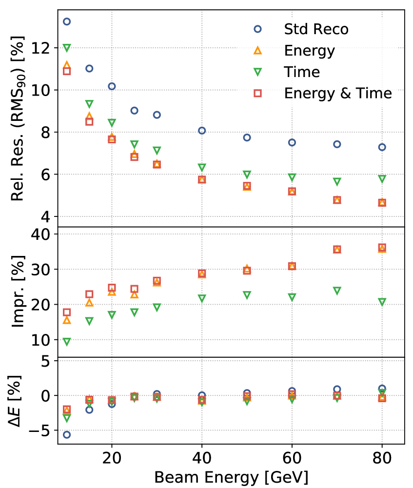
(a) Global software compensation

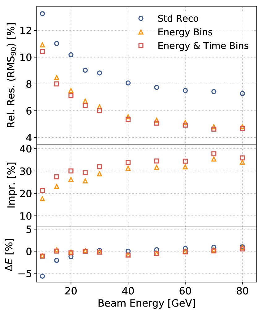
(b) Local software compensation

Figure 5: Results of using (a) global and (b) local software compensation using different observables compared to the standard reconstruction.

In Figure 6 the global and local version of the time assisted software compensation methods are compared. Besides the highest energy of $80\text{\,}\mathrm{GeV}$ where both methods show the same performance, the local approach gives better results with about a $5\text{\,}\mathrm{\char 37\relax}$ higher improvement over the standard reconstruction for most energies. These results reflect the observation that the local approach to software compensation is making better use of the additional time information.

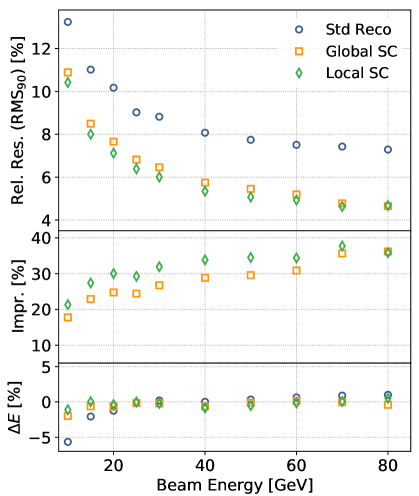
Figure 6: Comparison of global and local software compensation using both energy and time observables.

5.1 Weights for Local Software Compensation

Figure 7 shows the weights used for the local software compensation approach which uses only one set of hit energy bins. The weights of the first four bins are above one for the whole energy range, meaning hit energies in these bins get weighted up. The weights for the other bins are consistently below one and therefore energy depositions in these bins are weighted down.

The weights for the local software compensation approach using two sets of hit energy bins is shown in Figure 8 for early and late hits. It can be seen that the low energy hits in the late bins are weighted up much more compared to the early energy bins. The late energy bins greater than $5\text{\,}\text{MIP}$ include only very few data samples, as high-energetic, late energy depositions are rare in the detector. It can be concluded that the improvement in the resolution of the energy reconstruction process for the time assisted local software compensation is due to the power of distinguishing early and late low-energetic energy depositions and the corresponding increased weighting of the late energy depositions.

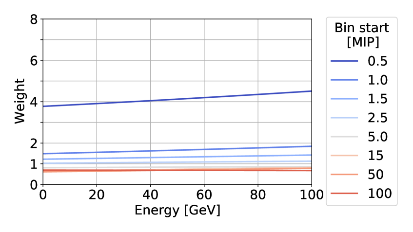
Figure 7: Weights for the local software compensation approach using only one set of energy bins. The different colors represent the weights for the different hit energy bins with the lower edge of the corresponding bin indicated in the legend.

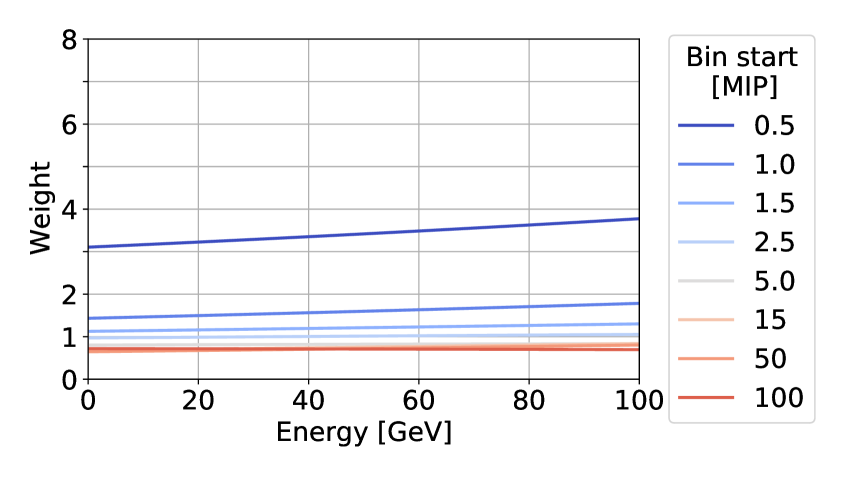
(a) Early hits

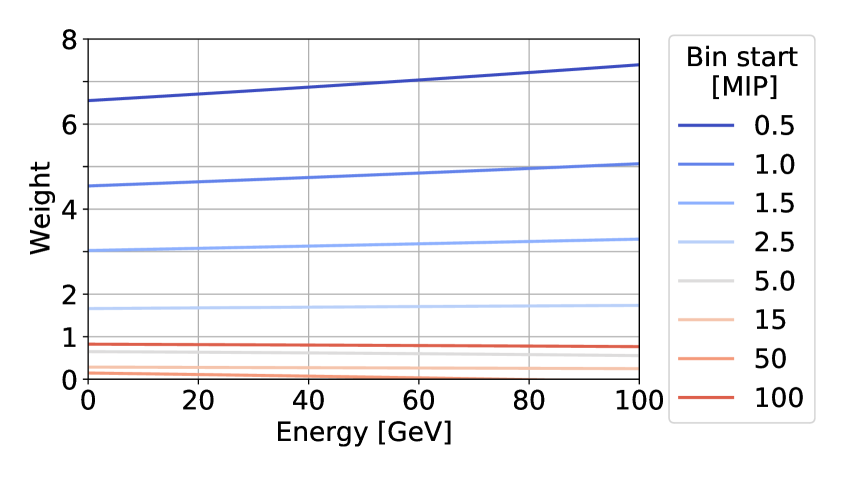
(b) Late hits

Figure 8: Weights for the local software compensation approach using energy bins for (a) early ($\leq$3\text{\,}\mathrm{ns}$$) and (b) late ($>$3\text{\,}\mathrm{ns}$$) hits. The different colors represents the weights for the different hit energy bins with the start of the corresponding bin indicated in the legend.

6 Impact of a limited time resolution

To explore the impact of the limited time resolution of $1\text{\,}\mathrm{n}\mathrm{s}$ on the performance of the reconstruction algorithms discussed here, the reconstruction methods are repeated assuming a perfect time resolution. In this case, the time of a calorimeter hit is given by the exact time of the first energy deposition in that particular cell in the simulations, without additional time smearing in the digitization step. All other digitization effects are applied. The parameters of the analysis, in particular the value of $3\text{\,}\mathrm{n}\mathrm{s}$ used to separate early and late shower components, are the same.

The results are shown in Figure 9. For global software compensation (9(a)) no improvement of the energy resolution can be observed with an ideal time resolution compared to a limited time resolution of $1\text{\,}\mathrm{ns}$. The energy resolution is dominated by the contribution of $C_{\text{global}}$. The more accurate time information does not add to a better performance. For local software compensation a clear improvement in energy resolution can be seen (9(b)). The improvement in energy resolution compared to the standard reconstruction increases by $2\text{\,}3\text{\,}$ percent points for energies below $50\text{\,}\mathrm{GeV}$. The better separation between early and late hits has a direct impact on the performance of the algorithm.

(a) Global software compensation

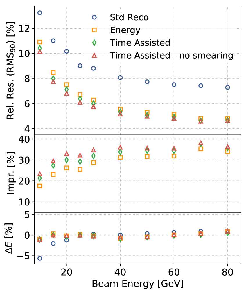
(b) Local software compensation

Figure 9: Results of (a) global and (b) local software compensation using different observables, and assuming a currently realistic time resolution of $1\text{\,}\mathrm{ns}$ and an ideal time resolution without time smearing, compared to the standard reconstruction.

7 Conclusions

Two methods of time assisted energy reconstruction within the CALICE AHCAL were presented and studied on simulated data. Both methods rely on the time structure of hadronic showers, where late hits are predominantly caused by late neutrons. Strong correlations of the fraction of late energy deposits with the reconstructed energy were observed. In a global software compensation approach these correlations have been exploited for an improved energy resolution compared to the standard reconstruction. However, the improvement is less than what can be achieved using an observable based on the hit energy distribution. The combination of both time and energy density observables does not lead to significant improvements over the purely energy-based methods. For a local software compensation approach the number of bins were doubled and weights have been derived separately for early and late energy depositions. With this approach, improvements in the energy resolution compared to the standard local software compensation approach using only energy density have been observed. Over most of the energy range, a better energy resolution than for the global software compensation has been achieved. A perfect time resolution enables additional improvements compared to a $1\text{\,}\mathrm{n}\mathrm{s}$ time resolution.

These results show that time information in highly-granular hadronic calorimeters, while correlated with information provided by energy density, is beneficial for energy reconstruction, in particular when local information on the cell level is used. Considering that the local software compensation technique introduced here uses only two bins in time, it is expected that more complex algorithms based on advanced machine-learning techniques which can use the full time information in a five-dimensional reconstruction (space, energy density, and time) will enable further improvements in energy reconstruction. Studies such as [22] give first impressions of this potential.

References

- [1] M. A. Thomson, Particle Flow Calorimetry and the PandoraPFA Algorithm, Nucl. Instrum. Meth. A 611 (2009) 25–40, [arXiv:0907.3577].
- [2] J.-C. Brient and H. Videau, The Calorimetry at the future e+ e- linear collider, eConf C010630 (2001) E3047, [arXiv:hep-ex/0202004].
- [3] V. L. Morgunov, Calorimetry design with energy-flow concept (imaging detector for high-energy physics), in CALOR 2002, Pasadena, California, 2002.
- [4] CALICE collaboration, C. Adloff et al., Construction and Commissioning of the CALICE Analog Hadron Calorimeter Prototype, JINST 5 (2010) P05004, [arXiv:1003.2662].
- [5] H. L. Tran, K. Krüger, F. Sefkow, S. Green, J. Marshall, M. Thomson et al., Software compensation in Particle Flow reconstruction, Eur. Phys. J. C 77 (2017) 698, [arXiv:1705.10363].
- [6] H. Abramowicz et al., The Response and Resolution of an Iron Scintillator Calorimeter for Hadronic and Electromagnetic Showers Between 10-GeV and 140-GeV, Nucl. Instrum. Meth. 180 (1981) 429.
- [7] H1 Calorimeter Group collaboration, B. Andrieu et al., Results from pion calibration runs for the H1 liquid argon calorimeter and comparisons with simulations, Nucl. Instrum. Meth. A 336 (1993) 499–509.
- [8] ATLAS Liquid Argon EMEC/HEC collaboration, C. Cojocaru et al., Hadronic calibration of the ATLAS liquid argon end-cap calorimeter in the pseudorapidity region 1.6 || 1.8 in beam tests, Nucl. Instrum. Meth. A 531 (2004) 481–514, [arXiv:physics/0407009].
- [9] CALICE collaboration, C. Adloff et al., Hadronic energy resolution of a highly granular scintillator-steel hadron calorimeter using software compensation techniques, JINST 7 (2012) P09017, [arXiv:1207.4210].
- [10] CALICE collaboration, F. Sefkow and F. Simon, A highly granular SiPM-on-tile calorimeter prototype, J. Phys. Conf. Ser. 1162 (2019) 012012, [arXiv:1808.09281].
- [11] L. Emberger, Analysis of Testbeam Data Recorded with the Large CALICE AHCAL Technological Prototype, in International Workshop on Future Linear Colliders, 5, 2021, arXiv:2105.08497.
- [12] WA78 collaboration, M. De Vincenzi et al., Experimental Study of Uranium Scintillator and Iron Scintillator Calorimetry in the Energy Range 135-GeV to 350-GeV, Nucl. Instrum. Meth. A 243 (1986) 348.
- [13] A. Caldwell, L. Hervas, J. A. Parsons, F. Sciulli, W. Sippach and L. Wai, Measurement of the time development of particle showers in a uranium scintillator calorimeter, Nucl. Instrum. Meth. A 330 (1993) 389–404.
- [14] D. Acosta et al., Electron - pion discrimination with a scintillating fiber calorimeter, Nucl. Instrum. Meth. A 302 (1991) 36–46.
- [15] N. Akchurin et al., Measurement of the Contribution of Neutrons to Hadron Calorimeter Signals, Nucl. Instrum. Meth. A 581 (2007) 643–650, [arXiv:0707.4019].
- [16] M. Frank, F. Gaede, C. Grefe and P. Mato, DD4hep: A Detector Description Toolkit for High Energy Physics Experiments, J. Phys. Conf. Ser. 513 (2014) 022010.
- [17] GEANT4 collaboration, S. Agostinelli et al., GEANT4–a simulation toolkit, Nucl. Instrum. Meth. A 506 (2003) 250–303.
- [18] M. Hirschberg, R. Beckmann, U. Brandenburg, H. Brueckmann and K. Wick, Precise measurement of Birks kB parameter in plastic scintillators, IEEE Trans. Nucl. Sci. 39 (1992) 511–514.
- [19] CALICE collaboration, B. Bilki et al., Pion and proton showers in the CALICE scintillator-steel analogue hadron calorimeter, JINST 10 (2015) P04014, [arXiv:1412.2653].
- [20] CALICE collaboration, C. Adloff et al., The Time Structure of Hadronic Showers in highly granular Calorimeters with Tungsten and Steel Absorbers, JINST 9 (2014) P07022, [arXiv:1404.6454].
- [21] CALICE collaboration, J. Repond et al., Hadronic Energy Resolution of a Combined High Granularity Scintillator Calorimeter System, JINST 13 (2018) P12022, [arXiv:1809.03909].
- [22] N. Akchurin, C. Cowden, J. Damgov, A. Hussain and S. Kunori, On the use of neural networks for energy reconstruction in high-granularity calorimeters, JINST 16 (2021) P12036, [arXiv:2107.10207].