Universal transport in periodically driven systems without long-lived quasiparticles

Abstract

An intriguing regime of universal charge transport at high entropy density has been proposed for periodically driven interacting one-dimensional systems with Bloch bands separated by a large single-particle band gap. For weak interactions, a simple picture based on well-defined Floquet quasiparticles suggests that the system should host a quasisteady state current that depends only on the populations of the system’s Floquet-Bloch bands and their associated quasienergy winding numbers. Here we show that such topological transport persists into the strongly interacting regime where the single-particle lifetime becomes shorter than the drive period. Analytically, we show that the value of the current is insensitive to interaction-induced band renormalizations and lifetime broadening when certain conditions are met by the system’s non-equilibrium distribution function. We show that these conditions correspond to a quasisteady state. We support these predictions through numerical simulation of a system of strongly interacting fermions in a periodically-modulated chain of Sachdev-Ye-Kitaev dots. Our work establishes universal transport at high entropy density as a robust far from equilibrium topological phenomenon, which can be readily realized with cold atoms in optical lattices.

I Introduction

The interplay of topology and far from equilibrium dynamics became an important arena of research in recent years Oka and Aoki (2009); Kitagawa et al. (2010); Lindner et al. (2011); Dalibard et al. (2011); Gómez-León and Platero (2013); Huse et al. (2013); Rudner et al. (2013); Dehghani et al. (2014); Foa Torres et al. (2014); Usaj et al. (2014); Chandran et al. (2014); Goldman et al. (2014); Grushin et al. (2014); Perez-Piskunow et al. (2015); Dal Lago et al. (2015); Nathan and Rudner (2015); Khemani et al. (2016); Von Keyserlingk and Sondhi (2016a, b); Else and Nayak (2016); Po et al. (2016); Potter et al. (2016); Eckardt (2017); Roy and Harper (2017a, b); Harper and Roy (2017); Gong et al. (2018); Esin et al. (2018); Ozawa et al. (2019); Cooper et al. (2019); Rudner and Lindner (2020a); Harper et al. (2020); Zhang and Yang (2021). In equilibrium, the field of topology has substantially influenced the modern understanding of electronic systems, contributing to the introduction of fundamental concepts such as topological robustness of quantum states, topological degeneracies of ground states, and non-abelian anyonic statistics Arovas et al. (1985); Altland and Zirnbauer (1997); Kitaev (2006); Stern (2008); Nayak et al. (2008); Kitaev (2009); Hasan and Kane (2010); Qi and Zhang (2011); Fidkowski and Kitaev (2011); Ren et al. (2016); Chiu et al. (2016); Wen (2017). Extension of these concepts to non-equilibrium systems provides the means for dynamical control of topological properties and design of topological phases “on-demand” Aidelsburger et al. (2011); Rechtsman et al. (2013); Aidelsburger et al. (2014); Jotzu et al. (2014); Fleury et al. (2016); Basov et al. (2017); Oka and Kitamura (2019); McIver et al. (2019); Shan et al. (2021); Mukherjee and Rechtsman (2021). Recently, periodic drives were employed to induce exotic phases of matter without equilibrium analogs Else et al. (2016); Titum et al. (2016); Peng et al. (2016); Zhang et al. (2017); Choi et al. (2017); Maczewsky et al. (2017); Mukherjee et al. (2017); Nathan et al. (2019); Wintersperger et al. (2020); Afzal et al. (2020); Esin et al. (2020, 2021).

Figure 1: The model and the single-particle spectrum. a Illustration of the system. A chain of atoms with time-modulated hopping and staggered potential, following the driving protocol realizing an adiabatic pump, as shown in the right bottom corner of panel a (we denote ${\Delta}d(t)=d_{+}(0,t)-d_{-}(0,t)$). In the numerical simulation, each site is an SYK dot with $N\to\infty$ orbitals that interact through random interactions [see Eq. (2)]. b The single-particle spectrum of the system at $t<0$, before the drive is switched on. The dashed line represents the Fermi level and the colored section represents initially occupied states, constituting a quarter of all the states in the system. The shaded gray areas show the instantaneous levels of the driven system in one period. The band structure is calculated for $J_{0}=1$, $J_{1}=0.85$, $v_{0}=2.55$, and ${\Omega}=0.5$ [see Eq. (1) for the definition of the single-particle Hamiltonian]. c The period averaged spectral function of the non-interacting system, $\bar{g}^{\Delta}(k;{\omega})$. Energy and frequency in panels b and c are plotted in units of $J_{0}=1$. d The period-averaged non-interacting density of states (DOS).

An important paradigmatic model of an intrinsically non-equilibrium topological system is the topological pump. The topological pump, originally introduced by Thouless Thouless (1983), describes a one-dimensional atomic chain with an adiabatically slowly and periodically in time modulated potential. Such a system when tuned to its topological phase, supports a robust quantized transport Niu and Thouless (1984); Niu (1990); Brouwer (1998); Switkes (1999); Altshuler and Glazman (1999); Chern et al. (2007); Xiao et al. (2010); Meidan et al. (2011); Wang et al. (2013). The precise quantization and robustness of adiabatic pumps to external perturbations makes them important candidates for applications in quantum metrology Keller et al. (1999); Piquemal et al. (2004); Blumenthal et al. (2007); Giblin et al. (2012); Pekola et al. (2013) and processing of quantum information Fletcher et al. (2013); Ubbelohde et al. (2014); Johnson et al. (2017). Adiabatic pumps were recently experimentally realized in photonic systems and cold atoms Kraus et al. (2012); Schweizer et al. (2016); Lohse et al. (2016); Nakajima et al. (2016); Zilberberg et al. (2018); Lohse et al. (2018); Cerjan et al. (2020); Nakajima et al. (2021); Jürgensen et al. (2021); Minguzzi et al. (2021).

The realization of topological pumps in metallic interacting systems is challenging due to an interplay of inter-particle interactions and the non-adiabatic evolution stimulated by the periodic drive. Such an interplay often results in an extensive generation of entropy and incessant heating up of the system to a featureless, high-entropy state Lazarides et al. (2014); D’Alessio and Rigol (2014); Ponte et al. (2015). The heating can be significantly slowed down in the high driving frequency regime or under special conditions, giving rise to a long-lived prethermal state Bukov et al. (2015); Eckardt and Anisimovas (2015); Abanin et al. (2015); Bukov et al. (2016); Kuwahara et al. (2016); Else et al. (2017); Abanin et al. (2017); Reitter et al. (2017); Mori (2018); Howell et al. (2019); Vogl et al. (2019); Kuhlenkamp and Knap (2020); Fleckenstein and Bukov (2021). Recently it was shown that a slowly driven topological pump in the weakly interacting limit can form a quasi steady state Lindner et al. (2017); Gulden et al. (2020); Gawatz et al. (2021). In this limit, the quasi-steady state can be understood heuristically on the level of free dynamics and weak scattering of particles in well-defined Floquet-Bloch bands. Notably, the quasi steady state hosts a universal current that depends only on the populations of the system’s Floquet-Bloch bands and their associated quasienergy winding numbers.

Here we show that the quasi-steady state persists into the strongly interacting regime where the single-particle scattering lifetime is shorter than the drive period. Furthermore, in this regime, the current exhibits a similar universal value as in the weakly interacting case, despite the absence of long-lived single-particle Floquet states. We support our analytical predictions through numerical simulations of a system of strongly interacting fermions in a periodically-modulated chain of Sachdev-Ye-Kitaev (SYK) Sachdev and Ye (1993); Kitaev ; Maldacena and Stanford (2016) dots. Our work demonstrates a new approach for numerically exact simulations of driven, strongly interacting chains of many sites, by specializing to SYK-type interactions. This method outperforms the conventional exact diagonalization methods that can be applied to significantly smaller systems. In turn, approximate methods such as Hilbert space decimation (i.e., the time-dependent density matrix renormalization group White and Feiguin (2004); Schollwöck (2005)), can not be applied here, because thermalization dynamics generates long-ranged correlations.

II Definition of the problem

In this work, we consider a one-dimensional bipartite chain of $L$ unit cells with periodic boundary conditions, hosting $N$ flavors of otherwise spinless fermions (see Fig. 1a). We label the two sublattices by $A$ and $B$, and denote the lattice constant by $a$. For simplicity of notation, throughout we set $\hbar=k_{B}=e=1$.

At times $t\geq 0$, the evolution of the system is described by the time-periodic Hamiltonian $\hat{\mathcal{H}}(t)=\sum_{k{\alpha}}\hat{\boldsymbol{c}}^{\dagger}_{k{\alpha}}H_{0}(k,t)\hat{\boldsymbol{c}}_{k{\alpha}}+\hat{\mathcal{H}}_{\rm int}$, where $H_{0}(k,t)$ denotes the time-periodic single particle Bloch Hamiltonian and $\hat{\mathcal{H}}_{\rm int}$ denotes the electron-electron interactions. Here, $\hat{\boldsymbol{c}}_{k{\alpha}}^{\dagger}=(\hat{c}_{A,k{\alpha}}^{\dagger},\hat{c}_{B,k{\alpha}}^{\dagger})$; $\hat{c}_{s,k{\alpha}}^{\dagger}=\frac{1}{\sqrt{L}}\sum_{j\in j_{s}}e^{ikaj/2}\hat{c}_{j{\alpha}}^{\dagger}$, where $\hat{c}^{\dagger}_{j{\alpha}}$ creates a fermion at a position $j$ with flavor index ${\alpha}$; $j_{s}$ includes all the odd (even) sites for $s=A(B)$. The single-particle Hamiltonian describes the Rice-Mele model Rice and Mele (1982) with time-periodically modulated parameters:

$$H_{0}(k,t)=\begin{pmatrix}v(t)-{\mu}_{0}&d(k,t)\\ d^{\ast}(k,t)&-v(t)-{\mu}_{0}\\ \end{pmatrix}.$$ (1)

Here, $d(k,t)=d_{+}(k,t)+d_{-}(k,t)$ and $d_{\pm}(k,t)=e^{\mp ika/2}[J_{0}\pm J_{1}\sin({\Omega}t)]$ and $v(t)=v_{0}\cos({\Omega}t)$, where ${\Omega}$ is the driving frequency and $v_{0}$, $J_{0}$, $J_{1}$ are constants. The chemical potential ${\mu}_{0}$ sets the average density of the fermions in the chain (see Fig. 1b). For $t<0$, the system is assumed to be in an equilibrium state with respect to the Hamiltonian $\hat{\mathcal{H}}(t=0)$, at inverse temperature ${\beta}_{0}$.

The interparticle interactions are described by the Hamiltonian

$$\hat{\mathcal{H}}_{\rm int}=\sum_{jj^{\prime}}\sum_{{\alpha}{\beta}{\gamma}{\delta}}U_{{\alpha}{\beta}{\gamma}{\delta}}(j,j^{\prime})\hat{c}_{j{\alpha}}^{\dagger}\hat{c}_{j{\beta}}\hat{c}_{j^{\prime}{\gamma}}^{\dagger}\hat{c}_{j^{\prime}{\delta}}+{\rm h.c.}$$ (2)

In our analytical study, we assume a single flavor, ${\alpha}=1$, and generic short-ranged interactions of characteristic strength $U_{{\alpha}{\beta}{\gamma}{\delta}}(j,j^{\prime})=U\chi(|j-j^{\prime}|)$, where $\chi(|j-j^{\prime}|)$ is a rapidly decaying dimensionless function of its argument, with $\chi(1)=1$. (Note that for a single species of fermions, the on-site interaction terms, $j=j^{\prime}$, do not contribute.) In the numerical study, we consider the limit of a large number of flavors, $N$, with $N\to\infty$, see Fig. 1a for an illustration. Particles of different flavors can locally interact through an SYK-type on-site interaction term, where we consider random and constant in space interactions with $\overline{U_{{\alpha}{\beta}{\gamma}{\delta}}(j,j^{\prime})}=0$ and $\overline{U_{{\alpha}{\beta}{\gamma}{\delta}}^{2}(j,j^{\prime})}={\delta}_{jj^{\prime}}U^{2}/N^{3}$, such that the system preserves invariance to translations for every realization of disordered couplings Chowdhury et al. (2018); Patel et al. (2018).

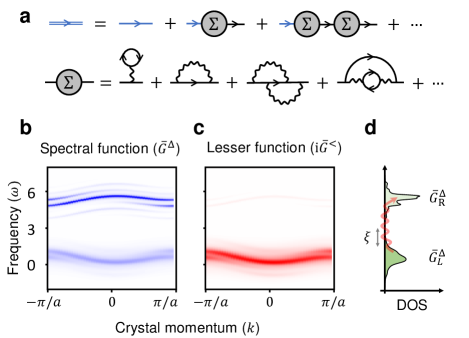
Figure 2: Renormalization of the spectrum by interactions. a First row: Dyson’s expansion for the band resolved Green’s function. The double and single blue lines indicate the band-resolved renormalized and bare functions respectively. Black lines denote the full bare Green’s function. Second row: Diagrammatic expansion of the self-energy, used in the analytical model (shown up to order $U^{2}$). In the numerics, we considered SYK interactions in the infinite $N$ limit, in which all the diagrams with odd number of interaction vertices or with crossed lines are averaged to zero (i.e., only the last diagram in a contributes). b Period-averaged spectral function, $\bar{G}^{\Delta}(k;{\omega})$, renormalized by the SYK interactions with $U=1$. c Period-averaged lesser function, $i\bar{G}^{<}(k;{\omega})$, indicating occupation after 30 periods of the drive, for the same parameters as in b. Note the weak, yet finite occupation of the upper band produced by the interband processes. d The renormalized period-averaged single-particle DOS. In the presence of interaction, the non-interacting DOS appearing in Fig. 1d, broadens obtaining exponential tails ${\xi}$. The broadening creates an overlap between the upper and lower bands, forming an interband heating channel (indicated by the wiggly arrow). Frequencies are plotted in units of $J_{0}=1$.

III Non-interacting dynamics

Before studying the interacting model, we briefly summarize the dynamics of the non-interacting topological pump Thouless (1983); Shih and Niu (1994); Xiao et al. (2010); Kitagawa et al. (2010); Lindner et al. (2017); Privitera et al. (2018). We initialize the pump in an equilibrium state of $\mathcal{H}(0)$, at inverse temperature ${\beta}_{0}$ and a chemical potential $\mu_{0}$ that fixes the average density of particles at $n_{0}$, see Fig. 1b. The spectral function is initially periodic in $k$, following the spectrum of the static Hamiltonian, $\mathcal{H}(0)$, as is demonstrated in Fig. 1b.

After switching on the drive (i.e., for $t>0$), the dynamics of the system follows the time-dependent Hamiltonian $\mathcal{H}(t)$. Shortly after the quench, the bands of high intensity in the spectral function develop a pronounced structure of sidebands, spaced by the drive frequency $\Omega$, and furthermore obtain nonvanishing net slopes Kitagawa et al. (2010) as a function of $k$ (see Fig. 1c and attached video). The peaks of the spectral function at each $k$ correspond to quasienergies associated with the single-particle Floquet state solutions Rudner and Lindner (2020b, a) of the time-periodic Rice-Mele problem, $[i\partial_{t}-H_{0}(k,t)]|{{\Psi}_{\nu}(k,t)}\rangle=0$, with the multiple values across the different sideband peaks capturing the indeterminacy of quasienergy up to integer multiples of the drive frequency, $\Omega$. The single particle Floquet states Shirley (1965); Sambe (1973) are given by $|{{\Psi}_{{\nu}}(k,t)}\rangle=e^{-i{\varepsilon}_{{\nu}}(k)t}\sum_{m}e^{-i{\Omega}mt}|{{\phi}_{{\nu}}^{m}(k)}\rangle$, where $\{|{{\phi}_{{\nu}}^{m}(k)}\rangle\}$ are time-independent states. Here, ${\varepsilon}_{{\nu}}(k)$ is the corresponding quasienergy of the single particle state with crystal momentum $k$, and chirality (or Floquet band) index $\nu=\{\text{L},\text{R}\}$ for the net left- and right-moving bands, respectively. We denote the bandwidth of the Floquet bands by $W_{F}$ and the gap between them by ${\Delta}$. The net chiralities of the bands are determined by the topological index Kitagawa et al. (2010); Rudner and Lindner (2020a) $\mathcal{W}={\Omega}^{-1}\oint dk\,\partial_{k}{\varepsilon}_{R/L}(k)=\pm 1$, where the $+$ ($-$) sign corresponds to the $R$ ($L$) band. The chiralities of the bands are exhibited by the spectral function shown in Fig. 1c. As the momentum changes from $k=-{\pi}/a$ to $k={\pi}/a$, the peaks of the spectral function of the $R$ ($L$) band shift in frequency from ${\omega}$ to ${\omega}\pm{\Omega}$.

IV Time-evolution towards the quasisteady state

We now study the dynamics of the system in the interacting case. In particular, we focus on the evolution of the two-point Green’s functions, providing information about expectation values of one-body operators, such as particle densities and the current (see below). The time-evolution of the interacting system’s two-point Green’s functions is described by the Kadanoff-Baym equations Baym and Kadanoff (1962)

$$[i\partial_{t}-H_{0}(t)]G^{R}(k;t,t^{\prime})=\delta(t-t^{\prime})+{\Sigma}^{R}\circ G^{R}$$ (3a)

$$[i\partial_{t}-H_{0}(t)]G^{<}(k;t,t^{\prime})={\Sigma}^{R}\circ G^{<}+{\Sigma}^{<}\circ G^{A},$$ (3b)

where for brevity we have suppressed the crystal momentum and time indices on the right hand sides of these equations, and the $\circ$ symbol indicates a convolution over time and matrix product in the sublattice indices. In Eq. (3), the (flavor-averaged) retarded and lesser Green’s functions are defined as $G^{R}_{ss^{\prime}}(k;t,t^{\prime})=-\frac{i}{N}{\theta}(t-t^{\prime})\sum_{{\alpha}=1}^{N}\overline{\langle\{\hat{c}_{s,k{\alpha}}(t),\hat{c}^{\dagger}_{s^{\prime},k{\alpha}}(t^{\prime})\}\rangle}_{{\rho}_{0}}$, and $G^{<}_{ss^{\prime}}(k;t,t^{\prime})=\frac{i}{N}\sum_{{\alpha}=1}^{N}\overline{\langle\hat{c}^{\dagger}_{s^{\prime},k{\alpha}}(t^{\prime})\hat{c}_{s,k{\alpha}}(t)\rangle}_{{\rho}_{0}}$, while $G_{ss^{\prime}}^{A}(k;t,t^{\prime})=G_{s^{\prime}s}^{R}(k;t^{\prime},t)^{\dagger}$. In these expressions, the expectation values are calculated with respect to the initial state described by the density matrix ${\rho}_{0}$, describing an equilibrium state with respect to $\mathcal{H}(0)$ with temperature ${\beta}_{0}$ and average density of particles $n_{0}$. The bar denotes averaging over the random interaction strength (in the case of the SYK interactions), “$\left\{,\right\}$” denotes an anticommutator, and ${\theta}(t)$ is the Heaviside step function. Throughout, we omit the sublattice indices $s,s^{\prime}$, leaving the $2\times 2$ matrix structure of the Green’s functions implicit. The retarded and lesser components of self-energy are denoted by ${\Sigma}^{R}(k;t,t^{\prime})$ and ${\Sigma}^{<}(k;t,t^{\prime})$, respectively (see Fig. 2a and Appendix C for technical details).

IV.1 Single-particle spectral function

The renormalized single-particle spectrum of the non-equilibrium system is encoded in the retarded Green’s function, whose time-evolution is given by Eq. (3a). In order to facilitate the separation of intraband and interband scattering processes below, we write the full retarded Green’s function as a sum of $R$- and $L$-band projected Green’s functions: $G^{R}=G_{R}^{R}+G_{L}^{R}$. The band-resolved Green’s functions are defined through the Dyson series shown in Fig. 2a, corresponding to Dyson’s equation,

$$\begin{split}&G^{R}_{{\nu}}(k;t,t^{\prime})=g^{R}_{{\nu}}(k;t,t^{\prime})+g^{R}_{{\nu}}\circ{\Sigma}^{R}\circ G^{R},\end{split}$$ (4)

where, as in Eqs. (3a) and (3b), we suppress the crystal momentum and time indices on the last term for brevity. Here, $g^{R}_{{\nu}}(k;t,t^{\prime})$ is the non-interacting retarded Green’s function projected to band $\nu$, see Appendix A for more details.

We define the renormalized band-resolved spectral functions as $G_{\nu}^{\Delta}(k;{\omega},\bar{t})=i[G_{\nu}^{R}(k;{\omega},\bar{t})-G_{\nu}^{A}(k;{\omega},\bar{t})]$, where $G_{\nu}^{R}(k;{\omega},\bar{t})$ is obtained via the Wigner transform of the two-time function, $G_{\nu}^{R}(k;t,t^{\prime})$, with $\bar{t}=\frac{1}{2}(t+t^{\prime})$, and $G_{\nu}^{A}(k;{\omega},\bar{t})=[G_{\nu}^{R}(k;{\omega},\bar{t})]^{\dagger}$. The renormalized band-resolved spectral function broadens due to interactions, with tails extending into the gap that decay approximately as $e^{-\omega/\xi}$. In what follows, we focus on the limit ${\xi}\ll{\Delta}$, where the band-resolved spectral functions are well separated in frequency, see Figs. 2b,d. This separation of the renormalized Floquet bands in the frequency domain is crucial for obtaining a long-lived quasi steady state in the system (see below).

The renormalization of the single-particle spectral function is caused by the dressing of the non-interacting Floquet bands by virtual electron-hole pair creation and annihilation processes. Our analytical estimate near the quasi steady state (see Appendix C) suggests that the broadening of $G^{\Delta}_{L}$ in the limit $W_{F}\ll U\ll{\Delta}$ is approximately given by ${\xi}_{\text{L}}\approx-W_{F}/\ln\left(\frac{U^{2}}{{\Delta}^{2}}[f^{0}_{L}\bar{f}^{0}_{L}+f^{0}_{R}\bar{f}^{0}_{R}]\right)$, where $f^{0}_{L}$ and $f^{0}_{R}$ are the occupation probabilities of the Floquet bands (see below) and $\bar{f}^{0}_{\nu}=1-f^{0}_{\nu}$.

IV.2 The kinetic equation and population dynamics

To study the formation and properties of the quasisteady state, we define occupation probabilities by parametrizing the lesser Green’s function as

$$G^{<}(k;t,t^{\prime})=f_{R}\circ G^{A}_{R}-G^{R}_{R}\circ f_{R}+f_{L}\circ G^{A}_{L}-G^{R}_{L}\circ f_{L},$$ (5)

where crystal momentum and time indices are suppressed on the right hand side. By analogy to the case of thermodynamic equilibrium, where the (Fourier-transformed) lesser Green’s function and the spectral function are related via the Fermi occupation function, in Eq. (5) the Hermitian matrices $f_{R}(k;t,t^{\prime})$ and $f_{L}(k;t,t^{\prime})$ play the roles of distribution functions for the two bands. As we will discuss further below, this interpretation is most meaningful when $f_{R}(k;t,t^{\prime})$ and $f_{L}(k;t,t^{\prime})$ take simple forms in terms of their matrix and time (or frequency) structures. We will see that such a simple form naturally emerges in the quasisteady state of the system.

To assess the dynamics of the distribution functions we derive a kinetic equation for $\partial_{\bar{t}}f_{L}(k;{\omega},\bar{t})$, where $f_{L}(k;{\omega},\bar{t})$ is obtained via the Wigner transform of the two-time function, $f_{L}(k;t,t^{\prime})$. A similar approach is often employed in studies of weakly interacting dynamical systems Rammer and Smith (1986); Rammer (2007); Kamenev (2011). Here, we generalize this approach to the strongly interacting case, without imposing the “on-shell” approximation Picano et al. (2021). Crucially, such an approximation would not correctly capture interband scattering, which occurs through high-order processes in $U$.

The kinetic equation is obtained by combining the Wigner transforms of Eqs. (5) and (3b) and subtracting terms proportional to $\partial_{\bar{t}}G^{R}(k;\omega,\bar{t})$, which itself is described by Eq. (3a) (see Appendix D for the full derivation). Generically, the kinetic equation for $f_{L}$ can be written as Genske and Rosch (2015) $\partial_{\bar{t}}f_{L}(k;{\omega},\bar{t})=\mathcal{I}_{L}(k;{\omega},\bar{t})\left\{f_{R},f_{L}\right\}$, where the collision integral $\mathcal{I}_{L}$ is a functional of $f_{R}$ and $f_{L}$ with a matrix structure in the sublattice indices. Notably, for values of ${\omega}$ where $G^{\Delta}_{L}(k;{\omega},t)$ has significant weight, i.e., near the lower band (see Fig. 2d), the net collision integral is exponentially small if its arguments are independent of $k$ and $\omega$ [see appendix D]: $f^{\rm(qs)}_{L}(k;{\omega},\bar{t})=f_{L}^{0}{\bf 1}$, $f^{\rm(qs)}_{R}(k;{\omega},\bar{t})=f_{R}^{0}{\bf 1}$, where $f_{L}^{0}$ and $f_{R}^{0}$ are constants and ${\bf 1}$ denotes the identity matrix in sublattice space. In particular, we estimate $\mathcal{I}_{L}\left\{f^{\rm(qs)}_{L},f^{\rm(qs)}_{R}\right\}\propto e^{-{\Delta}/{\xi}}{\delta}f$, where ${\delta}f=f_{R}^{0}-f_{L}^{0}$. A state described by this form of $f^{\rm(qs)}_{\nu}$, characterized by uniform occupation within each band, exhibits exponentially slow population dynamics and thus describes a long-lived quasisteady state of the system.

IV.3 Universal value of the current

Using the form of the quasisteady state found above in terms of two-point Green’s functions, we can now characterize observables in the quasisteady state. In particular we focus on the value of the time-averaged current, which was previously conjectured to take a universal value based on a weak-coupling picture and evidence from numerical simulations on modestly-sized systems.

The instantaneous current averaged along the chain in a generic translation-invariant state described by $G^{<}$ reads

$$\mathcal{J}(t)=-i\int\frac{dk}{2{\pi}}\mathrm{Tr}\left\{\partial_{k}H_{0}(k,t)G^{<}(k;t,t+0^{+})\right\},$$ (6)

where the momentum integral is performed over the first Brillouin zone. Next, we evaluate Eq. (6) in the quasisteady state given by $G_{\rm(qs)}^{<}(k;t,t^{\prime})=if_{R}^{0}G_{R}^{\Delta}(k;t,t^{\prime})+if_{L}^{0}G_{L}^{\Delta}(k;t,t^{\prime})+\mathcal{O}(e^{-\Delta/\xi})$ [see Eq. (5) and the following discussion]. At equal times, $G_{\rm(qs)}^{<}$ can be further simplified using $G^{\Delta}_{\nu}(k;t,t+0^{+})=g^{\Delta}_{\nu}(k;t,t+0^{+})$, due to the fact that the time-integrals in Eq. (4) vanish for $t=t^{\prime}$. Substituting the resulting quasisteady state form of $G_{\rm(qs)}^{<}$ into Eq. (6), we obtain $\mathcal{J}(t)=f^{0}_{R}\mathcal{J}_{R}^{0}(t)+f^{0}_{L}\mathcal{J}_{L}^{0}(t)$, where $\mathcal{J}^{0}_{\nu}=\int\frac{dk}{2{\pi}}\langle{{\Psi}_{\nu}}|{\partial_{k}H_{0}}|{{\Psi}_{\nu}}\rangle$ is the current carried by Floquet band $\nu$ of the system in the absence of interactions, when fully filled (see Appendix A). As defined in Sec. III above, $|{{\Psi}_{\nu}(k,t)}\rangle$ denotes the single-particle Floquet state with crystal momentum $k$ in band $\nu$ of system in the absence of interactions. In the adiabatic limit, the period averaged current $\bar{\mathcal{J}}^{0}_{{\nu}}=\frac{1}{T}\int_{0}^{T}dt\mathcal{J}^{0}_{{\nu}}$ is quantized Thouless (1983) as $\bar{\mathcal{J}}^{0}_{R,L}=\pm\frac{1}{T}$. In a system where the upper ($R$) band is initially empty and the lower ($L$) band has fractional filling ${\nu}_{0}=an_{0}$, we therefore expect $f_{L}^{0}={\nu}_{0}$ and $f_{R}^{0}=0$, such that the current in the quasisteady state is equal to $\bar{\mathcal{J}}^{(qs)}=\frac{{\nu}_{0}}{T}+\mathcal{O}(e^{-\Delta/\xi})$, where the correction captures the deviation of the quasi steady state from the maximal entropy state in which the upper band is empty.

This is a remarkable result: even in a limit where the single particle scattering lifetime may be short compared with the driving period, where the single particle Floquet states and associated spectrum are not well-resolved or defined, the current still attains a universal value associated with the nontrivial topology of the system’s single-particle Floquet spectrum in the absence of interactions. The universal value of current holds, up to an exponentially small correction, provided that the scattering rate (and associated level broadening, captured by $\xi$) remains small compared with the single particle band gap, $\Delta$.

Figure 3: Relaxation to the quasi steady state. a “Distance” to equilibrium, $\mathcal{D}_{\rm eq}(t)$, defined in Eq. (7), as a function of time. Lines of different colors in this and following panels correspond to the different interaction strengths indicated on the top of the figure, in units of $J_{0}=1$. Shaded areas indicate error bars due to the extrapolation procedure, see text. At $t=0$, the extrapolation yields non-physical, negative values of $\mathcal{D}_{\rm eq}(t)$ due to the quench, we thus cut-off these values in the plot. b Effective temperature of the lower band minimizing $\mathcal{D}_{\rm eq}(t)$ in units of $J_{0}=1$, as a function of time. Blue dashed line indicates the point where $T_{\rm eff}=W_{\text{F}}$. c Entropy density of the system’s one-body reduced density matrix as a function of time, defined in Eq. (8). A dashed line indicates maximal entropy for a quarter-filled system, when all the particles occupy the lower band. d Period averaged current normalized by the total density of particles and driving frequency, $\bar{\mathcal{J}}(t)(T/{\nu}_{0})$ as a function of time.

V Numerical analysis

To benchmark our analytical results, we numerically simulated the model given in Eqs. (1) and (2), with SYK interactions. In addition to the terms described above, we also included a weak random quadratic term $\hat{\mathcal{H}}_{\rm SYK-2}=\sum_{j,{\alpha}{\beta}}K_{{\alpha}{\beta}}\hat{c}_{j{\alpha}}^{\dagger}\hat{c}_{j{\beta}}+{\rm h.c.}$, where $\overline{K_{{\alpha}{\beta}}}=0$ and $\overline{K_{{\alpha}{\beta}}^{2}}=K^{2}/N$, with $K=0.05$. This additional term is essential for stabilizing the numerics in the weakly interacting regime.

The unique structure of the SYK interactions allows us to simulate considerably larger systems compared to exact diagonalization methods applied to systems with conventional interactions. Here, we simulated the time evolution of a chain of $100$ SYK dots arranged into $L=50$ unit cells. We used the Kadanoff-Baym equations [given in Eq. (3)] to evolve the Keldysh-ordered Green’s functions in time Stan et al. (2009); Eberlein et al. (2017); Bhattacharya et al. (2019); Kuhlenkamp and Knap (2020); Maldacena and Milekhin (2021); for further details see Appendix E. The system is initialized in an equilibrium state of $\hat{\mathcal{H}}(0)$ with temperature ${\beta}_{0}^{-1}=0.1$ and ${\mu}_{0}=-2.93$, which is set to fix the density of electrons approximately at quarter filling, see Fig. 1b. For the model itself, we select the parameter values: $J_{0}=1$, $J_{1}=0.85$, $v_{0}=2.55$, ${\Omega}=0.5$, see Eq. (1) and surrounding text for the definitions of the Hamiltonian and its parameters. We note that all the energies and frequencies are given in units in which $J_{0}=1$.

The time-evolution algorithm is based on the discretization of the time and frequency domains, with small steps ${\delta}t$ and ${\delta}{\omega}$, respectively. We performed the evolution for several values of steps in the range $0.08\leq\delta t\leq 0.16$ and $0.015\leq\delta\omega\leq 0.04$, and performed a two-dimensional linear extrapolation to ${\delta}t={\delta}{\omega}=0$. In the numerical results we present the extrapolated values with error bars indicating the uncertainty of the extrapolation procedure (defined as the difference between the extrapolated value and the closest numerically-determined point).

V.1 Formation of the quasisteady state

We first analyze the formation of the quasisteady state, wherein the distribution functions $f_{L}$ and $f_{R}$ for the two bands become independent of crystal momentum and frequency, while the total populations of the two bands remain approximately constant. As a means of characterizing the nonequilibrium state of the system, and to enable the extraction of an effective temperature (when it is appropriate to do so), we define the “distance” of the distribution from a thermal equilibrium state as

$$\mathcal{D}_{\rm eq}(\bar{t})=\min_{{\beta},{\mu}}\int\frac{a\cdot dk}{2{\pi}}\int_{-\infty}^{{\omega}_{c}}\frac{d{\omega}}{2{\pi}}{\rm Tr}\left|i\overline{G}^{<}+f_{\rm FD}({\beta},{\mu})\overline{G}^{\Delta}\right|,$$ (7)

where ${\omega}_{c}$ is the center of the spectrum and the Green’s functions are evaluated in the Wigner transformed representation and averaged over one period: $\overline{G}^{<}(k;\omega,\bar{t})\equiv\frac{1}{T}\int_{-T/2}^{T/2}ds\,G^{<}(k;\omega,\bar{t}+s)$ and similarly for $\overline{G}^{\Delta}(k;\omega,\bar{t})$. Here, $f_{\rm FD}({\beta},{\mu})=[1+e^{{\beta}({\omega}-{\mu})}]^{-1}$ is the Fermi function. For a system in thermal equilibrium, the integrand in Eq. (7) vanishes for all $k$ and $\omega$, corresponding to $\mathcal{D}_{\rm eq}=0$.

In Figs. 3a,b we plot the evolution of the distance to equilibrium $\mathcal{D}_{\rm eq}(\bar{t})$ and the extracted effective temperature $T_{\rm eff}={\beta}_{\rm min}^{-1}$, corresponding to the minimization in Eq. (7). When the drive is switched on at $t=0$, $\mathcal{D}_{\rm eq}$ rapidly grows, indicating evolution into a far from equilibrium state. Following the rapid rise, the system relaxes to the quasisteady state, which is manifested by the decay of $\mathcal{D}_{\rm eq}$. In parallel, the effective temperature grows approximately exponentially with a rate ${\Gamma}_{\rm intra}$: $T_{\rm eff}\sim{\beta}_{0}^{-1}e^{{\Gamma}_{\rm intra}t}$ (Fig. 3b). The quasisteady state observed in the simulation approximately realizes the conditions discussed in Sec. IV.2, once the effective temperature exceeds the width of the single-particle Floquet bands, $T_{\rm eff}\gg W_{\text{F}}$, indicated by blue dashed line (and for $\mathcal{D}_{\rm eq}\ll 1$). The curves of different colors in Figs. 3a,b correspond to different interaction strengths, $U$; the time to reach the quasisteady state rapidly decreases with interaction strength, $U$.

To track the system’s evolution towards a high entropy density state, we calculated the average von-Neumann entropy density of the system’s one-body reduced density matrix

$$S(\bar{t})=-{\rm Tr}\int\frac{dk}{2{\pi}}\left[(-i\overline{G}^{<})\log(-i\overline{G}^{<})+(i\overline{G}^{>})\log(i\overline{G}^{>})\right],$$ (8)

where $\bar{G}^{>}=-i\bar{G}^{\Delta}+\bar{G}^{<}$ and the Green’s functions are evaluated at equal times $t=t^{\prime}=\bar{t}$, see Fig. 3c. The value of $S(\bar{t})$ for a maximal entropy density state in a quarter-filled system, subject to the constraint that all the particles occupy the lower band, is given by $S^{\rm max}_{L}=\log(2)/a$. As can be seen in Fig. 3c, the entropy density stabilizes slightly above this value due to a small population excited to the upper band at $t=0$. After stabilizing near $S(t)\approx S^{\rm max}_{L}$, the entropy slowly grows further due to interband transitions. In the infinite time limit, we expect $S\to S^{\rm max}\approx 1.12/a$ corresponding to one quarter filling of the entire system.

In Fig. 3d, we extracted the period-averaged current normalized by the filling, $\bar{\mathcal{J}}/{\nu}_{0}$ [see Eq. (6)]. As follows from the discussion below Eq. (6), we expect an approximately quantized value in the units of $T^{-1}$ for the normalized current in the quasisteady state. Fig. 4b shows the period-averaged current normalized by ${\nu}_{0}$ as a function of the stroboscopic time. The gray strips indicate the uncertainty intervals associated with the extrapolation to infinitesimal grid spacing in the simulations, as described above. In the regime of strong interactions, the average current rapidly increases on a timescale set by $\sim{\Gamma}_{\rm intra}$. When the quasisteady state is reached, the current obtains the expected universal value to within the uncertainties of the numerical simulation, as expected. For later times, the current slowly decays with the rate ${\Gamma}_{\rm inter}$ due to interband heating. In the weakly interacting case, the normalized current remains non-universal for much longer times; for these cases, the quasisteady state was not reached within the time window that we were able to simulate. Interestingly, slowly-driven Fermi liquids have been shown to persist in non-thermal states for parametrically long timescales Kuhlenkamp and Knap (2020). The connection between the slow intraband heating observed here and the mechanism in Ref. Kuhlenkamp and Knap, 2020 will be interesting to investigate in future work.

V.2 Interband heating and universal current

To investigate the interband scattering processes and measure their rates, in Fig. 4a we extracted the density of excitations in the (renormalized) $R$ band from our simulations. We define the excitation density as $n_{\rm ex}(\bar{t})=-i\int_{\omega_{c}}^{\infty}\frac{d{\omega}}{2{\pi}}\int\frac{dk}{2\pi}{\rm Tr}\left\{G^{<}(k;{\omega},\bar{t})\right\}$. The period-averaged density of excitations jumps at $\bar{t}=0$, when the drive is switched on Privitera et al. (2018), and then gradually increases with an approximately constant rate ${\Gamma}_{\rm inter}$. The interband equilibration rate, ${\Gamma}_{\rm inter}$, compared to the intraband equilibration rate, ${\Gamma}_{\rm intra}$, is shown as a function of the interaction strength in Fig. 4b.

Fig. 2c shows the period averaged lesser Green’s function as a function of momentum and frequency, after $30$ periods of the drive. The excited population can be seen as a pale strip at the location of the upper band. Note that the features are heavily broadened due to fast intraband scattering, such that for the selected parameters the Floquet harmonic side bands are nearly completely washed out.

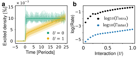
Figure 4: Heating and current in the quasi steady state. a Density of electrons excited to the upper band as a function of time, in the interacting and non-interacting cases. Circles represent the period averaged density. In the interacting case, the density of excitations increases with an approximately constant rate ${\Gamma}_{\rm inter}$, while in the non-interacting case the average charge is constant, following an initial jump at $t=0$. b Intraband (${\Gamma}_{\rm intra}$) and interband (${\Gamma}_{\rm inter}$) equilibration rates as a function of the interaction strength. The intraband equilibration rate is extracted from the temperature growth [see Fig. 3b]. The interband equilibration rate is extracted from the slope of the period-averaged excitation density, in a.

VI Discussion and outlook

Periodically driven systems can host Floquet-Bloch bands with unique topological properties that cannot be obtained in equilibrium systems. In the presence of interactions, it is natural to wonder if rapid scattering on timescales comparable to the driving period might mask any dynamical features expected to arise from the single-particle Floquet states. In this work we showed that this need not be the case: even in a state with high entropy density and rapid scattering, universal transport associated with the topological properties of the system’s Floquet Bloch bands persists. We demonstrated this phenomenon in the context of a topological pump with non-integer filling, which exhibits a long-lived quasisteady state with maximal entropy density (subject to the constraint of fixed particle number in each band). We derived conditions under which the quasisteady state hosts quantized transport (in units of the particle density), up to an exponentially small correction in the ratio of the system’s band gap to its renormalized band width.

To support these arguments, we studied this phenomenon numerically in an SYK-type chain. This setup enabled us to examine the dynamics in a regime of strong scattering, in system sizes much larger than could be accessed by exact evolution. This advantage is gained from the fact that the SYK system can be solved by time evolution of the Kadanoff-Baym equations. Our numerical results allowed us to study the dynamics leading to the formation of the quasisteady state. Importantly, we showed that quantized transport persists even when quasiparticles are short-lived due to fast intraband scattering and the Floquet sidebands are hence not well resolved.

VII Acknowledgments

We would like to thank Ervand Kandelaki and Michael Knap for illuminating discussions, and David Cohen and Yan Katz for technical support. N. L. acknowledges support from the European Research Council (ERC) under the European Union Horizon 2020 Research and Innovation Programme (Grant Agreement No. 639172), and from the Israeli Center of Research Excellence (I-CORE) “Circle of Light”. M. R. gratefully acknowledges the support of the European Research Council (ERC) under the European Union Horizon 2020 Research and Innovation Programme (Grant Agreement No. 678862) and the Villum Foundation. M. R. and E. B. acknowledge support from CRC 183 of the Deutsche Forschungsgemeinschaft. G.R. acknowledges support from the U.S. Department of Energy, Office of Science, Basic Energy Sciences under Award desc0019166 and the Simons Foundation.

Appendix A The band-resolved bare Green’s function

Here, we present the derivation of the retarded band-resolved bare Green’s function, see Fig. 1c,d. In the non-interacting case the flavors (denoted by ${\alpha}$ in Eq. (2)) are independent of each other. We thus focus on ${\alpha}=1$ and omit the flavor index. The bare retarded Green’s function is defined as

$$g^{R}_{ss^{\prime}}(k;t,t^{\prime})=-i\langle\{\hat{c}_{s,k}(t),\hat{c}_{s^{\prime},k}^{\dagger}(t^{\prime})\}\rangle{\theta}(t-t^{\prime}),$$ (9)

where $s,s^{\prime}=\{A,B\}$ are the sublattice indices, and $\hat{c}_{s,k}(t)=\hat{U}^{\dagger}(t)\hat{c}_{s,k}(0)\hat{U}(t)$. The unitary evolution operator is given by $\hat{U}(t)=\mathcal{T}e^{-i\int_{-\infty}^{t}\hat{\mathcal{H}}(t^{\prime})dt^{\prime}}$, where $\hat{\mathcal{H}}(t)$ is given in Eq. (1). For $t$ and $t^{\prime}$ well after the quench, the time-dependent Hamiltonian can be diagonalized, by the Floquet eigenstates $|{{\Psi}_{\nu}(k,t)}\rangle$, for ${\nu}=R,L$. In this eigenbasis the fermionic operators read

$$\hat{c}_{s,k}(t)=\langle{s}|{{\Psi}_{R}(k,t)}\rangle\hat{d}_{R,k}+\langle{s}|{{\Psi}_{L}(k,t)}\rangle\hat{d}_{L,k},$$ (10)

where $\hat{d}_{{\nu},k}$ annihilate the Floquet state $|{{\Psi}_{\nu}(k,t)}\rangle$ and $\langle{s}|{{\Psi}_{\nu}(k,t)}\rangle$ is the amplitude of the Floquet state projected onto a sublattice $s$. Substituting Eq. (10) in Eq. (9), and evaluating $\langle\{\hat{d}^{\dagger}_{{\nu},k},\hat{d}_{{\nu}^{\prime},k}\}\rangle={\delta}_{{\nu}{\nu}^{\prime}}$, we arrive at

$$\begin{split}&g^{R}_{ss^{\prime}}(k;t,t^{\prime})=-i{\theta}(t-t^{\prime})\times\\ &\left[\langle{s}|{{\Psi}_{R}(k,t)}\rangle\langle{{\Psi}_{R}(k,t^{\prime})}|{s^{\prime}}\rangle+\langle{s}|{{\Psi}_{L}(k,t)}\rangle\langle{{\Psi}_{L}(k,t^{\prime})}|{s^{\prime}}\rangle\right].\end{split}$$ (11)

Following Eq. (11), we define the right/left chirality Green’s functions as

$$\begin{split}&g^{R}_{{\nu}}(k;t,t^{\prime})=-i{\theta}(t-t^{\prime})|{{\Psi}_{\nu}(k,t)}\rangle\langle{{\Psi}_{\nu}(k,t^{\prime})}|.\end{split}$$ (12)

Note, that $g^{R}_{{\nu}}(k;t,t^{\prime})$ is essentially a projector to one of the Floquet bands and therefore has a matrix structure in the sublattice indices. The original Green’s function [defined in Eq. (9)] is given by the sum of the band-resolved Green’s functions, $g^{R}_{ss^{\prime}}(k;t,t^{\prime})=\langle{s}|{g^{R}_{R}(k;t,t^{\prime})+g^{R}_{L}(k;t,t^{\prime})}|{s^{\prime}}\rangle$.

A.1 Wigner representation of the retarded Green’s function

Next, we derive the Winger-transformed representation of the band-resolved Green’s function, given in Eq. (12). The Wigner transform of $g(k;t,t^{\prime})$ is defined as

$$g(k;{\omega},\bar{t})=\int e^{i{\omega}{\delta}t}g(k;\bar{t}+{\delta}t/2,\bar{t}-{\delta}t/2)d{\delta}t.$$ (13)

To evaluate Eq. (13), we substitute the harmonic expansion of the Floquet states, $|{{\Psi}_{{\nu}}(k,t)}\rangle=e^{-i{\varepsilon}_{{\nu}}(k)t}\sum_{m}e^{-i{\Omega}mt}|{{\phi}_{{\nu}}^{m}(k)}\rangle$ (see Sec. IV) in Eq. (12). We then perform the ${\delta}t$ integral yielding Kitagawa et al. (2011)

$$g^{R}_{{\nu}}(k;{\omega},\bar{t})=\sum_{m,n}\frac{|{{\phi}_{{\nu}}^{m+n}(k)}\rangle\langle{{\phi}^{m-n}_{{\nu}}(k)}|}{{\omega}-{\varepsilon}_{{\nu}}(k)+m{\Omega}+i0^{+}}e^{-2in{\Omega}\bar{t}}.$$ (14)

The period averaged Green’s function [cf. Fig. 1c] can be extracted from the $n=0$ terms in Eq. (14), yielding

$$\bar{g}^{R}_{{\nu}}(k;{\omega})=\sum_{m}\frac{|{{\phi}_{{\nu}}^{m}(k)}\rangle\langle{{\phi}^{m}_{{\nu}}(k)}|}{{\omega}-{\varepsilon}_{{\nu}}(k)+m{\Omega}+i0^{+}}.$$ (15)

Appendix B Definition of the Keldysh-Floquet Green’s functions in the gauge-invariant form

Due to the non-equilibrium nature of the Floquet-Keldysh Green’s functions, the energy in the collision processes is only conserved modulo ${\Omega}$. This property complicates the calculations using the Keldysh formalism, as multiple photon absorption/emission processes have to be take in account in each collision. Here, we present a gauge invariant definition of the Green’s functions in which the ${\omega}$ index is conserved in the collision processes, and show how convolution and product of the the two-time Green’s functions are defined with this gauge choice. Such a definition, allows us to operate the Keldysh-Floquet Green’s functions as equilibrium Keldysh Green’s functions with additional matrix structure in the Floquet harmonics.

Given the Wigner-transformed Green’s function $G({\omega},\bar{t})$ [see Eq. (13) for definition], we define the Green’s function in the harmonic basis (with indices $m,n\in\mathbb{Z}$) as

$$G_{mn}({\omega})=\frac{1}{T}\int_{0}^{T}d\bar{t}G({\omega}+\frac{m+n}{2}{\Omega},\bar{t})e^{i{\Omega}(m-n)\bar{t}}.$$ (16)

This definition is invariant under the transformation $G_{m,n}({\omega}+l{\Omega})=G_{m+l,n+l}({\omega})$ for any integer $l$. A convolution $C(t,t^{\prime})=\int dsA(t,s)B(s,t)$, reads

$$C_{mn}({\omega})=\sum_{l}A_{ml}({\omega})B_{ln}({\omega}).$$ (17)

Similarly, a product of two same-time functions, $P(t,t^{\prime})=A(t,t^{\prime})B(t,t^{\prime})$ is given by

$$P_{mn}({\omega})=\sum_{l}\int\frac{d{\omega}^{\prime}}{2{\pi}}A_{m-l,n}({\omega}-{\omega}^{\prime})B_{l,0}({\omega}^{\prime}).$$ (18)

Appendix C Evaluation of the self-energy and renormalization of the spectral function

Here, we estimate the broadening ${\xi}$ of the renormalized bandwidth of the Floquet bands, discussed in Sec. IV.1. In all the expressions in this section, we assume the Green’s functions in the frequency domain are defined as matrices in the harmonic basis [as defined in Eq. (16)], and implicitly contract the harmonic indices following the rules given in Eqs. (17) and (18). The renormalization of the spectral width can be understood from the definition of the renormalized Green’s function in terms of the bare one,

$$[G^{R}({\omega})]^{-1}=[g^{R}({\omega})]^{-1}-{\Sigma}^{R}({\omega}),$$ (19)

following from Eq. (3a). Focusing on the values of ${\omega}$ at the gap of the bare function, i.e., where $g^{\Delta}({\omega})=0$, the renormalized spectral function reads

$$G^{\Delta}({\omega})\approx-[g^{R}({\omega})]^{2}{\Sigma}^{\Delta}({\omega}).$$ (20)

Therefore, to estimate the broadening of the spectral function, we need to estimate ${\Sigma}^{\Delta}({\omega})$. In what follows, we estimate the lesser and greater components of the self-energy ${\Sigma}^{\lessgtr}({\omega})$, constituting the spectral component, ${\Sigma}^{\Delta}=i{\Sigma}^{>}-i{\Sigma}^{<}$.

To estimate the self-energy, we need to sum over all irreducible diagrams allowed by the interaction term (first four terms in the expansion are demonstrated Fig. 2a). We begin by estimating the greater component of the self-energy, ${\Sigma}^{>}({\omega})$. Consider a generic irreducible diagram in this sum, corresponding to the order $U^{p}$ in the interaction strength, see Fig. 5. Such a diagram contains $p$ interaction vertices evaluated at the times $t_{1}$, $t_{2}$,.., $t_{p}$ and positions on the Keldysh contour $i_{1},..,i_{p}$, where $i_{p}=\pm$ corresponding to positive ($+$) and negative ($-$) branches on the Keldysh contour. The vertices are connected by the non-interacting propagators $g_{i,i^{\prime}}(t,t^{\prime})$, with the convention $g_{+-}=g^{<}$, $g_{-+}=g^{>}$, $g_{++}=g^{T}$ and $g_{--}=g^{\tilde{T}}$. For a specific combination of $i_{p}$, it is useful to arrange the diagram such that all the vertices on the positive branch are on the left side and all the vertices on the negative branch are on the right side, see Fig. 5. Notice that by the definition of ${\Sigma}^{>}$ the incoming vertex belongs to the negative Keldysh branch and the outgoing vertex belongs to the positive branch.

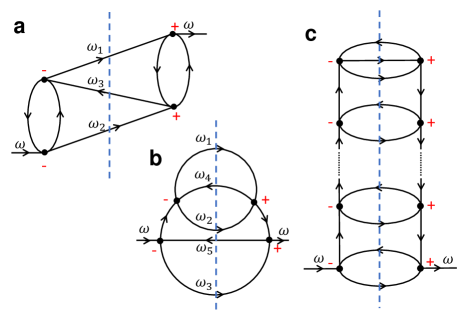
Figure 5: Examples of diagrams contributing to the self energy, ${\Sigma}^{>}({\omega})$, arranged such that the vertices on the positive Keldysh branch are at the left side and the vertices on the negative Kelysh branch are at the right side. Notice that the left diagram would not contribute in the case of the SYK interactions, since it is subleading in the number of the SYK flavours.

Next, we transform the expression for the self energy following the transformation given in Eq. (16). For convenience, we enumerate the frequencies of the $l$ propagators going from the left to the right side of the diagram by ${\omega}_{1}$, ${\omega}_{2}$,…, ${\omega}_{l}$, and $l-1$ propagators going from the right side to the left side by ${\omega}_{l+1}$, ${\omega}_{l+2}$,…, ${\omega}_{2l-1}$. The maximal value of $l$ is limited by $p$. We define the sum of the frequencies of the propagators crossing the center of the diagram with opposite signs by ${\Delta}{\omega}={\omega}_{1}+...+{\omega}_{l}-{\omega}_{l+1}-...-{\omega}_{2l-1}$. From the conservation of frequency, ${\Delta}{\omega}={\omega}$, where ${\omega}$ is the frequency associated with self-energy.

By construction, the propagators directed from the left to right correspond to the greater component of the Green’s function, $g^{>}({\omega}_{1})$,…, $g^{>}({\omega}_{l})$ while the ones directed oppositely correspond to the lesser components of the Green’s function, $g^{<}({\omega}_{l+1})$,…, $g^{<}({\omega}_{2l-1})$. For simplicity, we suppressed the momentum dependence and the Floquet harmonic indices, as they are not important for the qualitative result. Therefore, the greater component of the self-energy of a single diagram to the order $U^{p}$ is given by

$$\begin{split}{\Sigma}_{p}^{>}({\omega})=&U^{p}\int\frac{d{\omega}_{1}...d{\omega}_{2l-1}}{(2{\pi})^{2l-1}}{\delta}({\omega}-{\Delta}{\omega})\times\\ &\times g^{>}({\omega}_{1})\dotsb g^{<}({\omega}_{2l-1})\mathcal{F}_{p}({\omega}_{1},...,{\omega}_{2l-1}).\end{split}$$ (21)

The function $\mathcal{F}_{p}$ includes the contribution from all the propagators that do not cross the center of the diagram, which include the time-ordered and anti time-ordered components. It is analytical and non vanishing, therefore can not change the support of the convolution in the ${\omega}$ domain, yet it may change the weight of the function.

Our goal is to estimate ${\Sigma}^{>}({\omega})$ for ${\omega}$ away from the support of the non-interacting density of states. The dominant contribution to the self-energy would arise from ladder-shaped diagram, as is shown in Fig. 5c. Such a diagram has maximal number of lines crossing the center of the diagram, with minimal constraints on the intermediate frequencies.

The unique topology of this diagram allows to write it as a recursive relation

$$\begin{split}{\Sigma}^{>}_{p+2}({\omega})=&U^{2}\int\frac{d{\omega}_{1}d{\omega}_{2}d{\omega}_{3}}{(2{\pi})^{2}}{\delta}({\omega}_{3}-{\omega}+{\omega}_{1}-{\omega}_{2})\times\\ &\times g^{>}({\omega}_{1})g^{<}({\omega}_{2})g^{T}({\omega}_{3})g^{\tilde{T}}({\omega}_{3}){\Sigma}^{>}_{p}({\omega}_{3}).\end{split}$$ (22)

with the initial condition

$$\begin{split}{\Sigma}^{>}_{2}({\omega})=&U^{2}\int\frac{d{\omega}_{1}d{\omega}_{2}}{(2{\pi})^{2}}g^{>}({\omega}_{1})g^{<}({\omega}_{2})g^{>}({\omega}-{\omega}_{1}+{\omega}_{2}).\end{split}$$ (23)

For simplicity, we assume a nearly quasi steady state in which the lesser and greater functions can be approximated by $g^{>}({\omega})\approx i\bar{f}^{0}_{R}g^{\Delta}_{R}({\omega})+i\bar{f}^{0}_{L}g^{\Delta}_{L}({\omega})$ and $g^{<}({\omega})\approx-if^{0}_{R}g_{R}^{\Delta}({\omega})-if^{0}_{L}g_{L}^{\Delta}({\omega})$. The dominant contribution arises from diagrams where each pair of propagators in Eqs. (22) and (23) corresponds to the same band, i.e., $g^{>}({\omega}_{1})g^{<}({\omega}_{2})\to(f_{L}\bar{f}_{L}+f_{R}\bar{f}_{R})g_{0}^{\Delta}({\omega}_{1})g_{0}^{\Delta}({\omega}_{2})$, where $g_{0}^{\Delta}({\omega})$, is the density of states of one of the bands shifted to the center of the energy. We also approximate $g^{T}({\omega})g^{\tilde{T}}({\omega})\approx 1/{\omega}^{2}$.

The solution to Eq. (23), can be written as ${\Sigma}_{2}^{>}({\omega})\approx iU^{2}(f_{L}\bar{f}_{L}+f_{R}\bar{f}_{R})[\bar{f}_{R}\tilde{g}^{\Delta}_{R}(3W_{F},{\omega})+\bar{f}_{L}\tilde{g}^{\Delta}_{L}(3W_{F},{\omega})]$, where $\tilde{g}^{\Delta}_{\nu}(d,{\omega})$ is a function of width $d$ centered around the ${\nu}$-th band. Applying Eq. (22), we obtain ${\Sigma}^{>}_{4}({\omega})\approx i\frac{U^{4}}{((3/2)W_{F})^{2}}(f_{L}\bar{f}_{L}+f_{R}\bar{f}_{R})^{2}[\bar{f}_{R}\tilde{g}^{\Delta}_{R}(5W_{F},{\omega})+\bar{f}_{L}\tilde{g}^{\Delta}_{L}(5W_{F},{\omega})]$. Similarly, after $p$ iterations, we arrive at ${\Sigma}^{>}_{2p}({\omega})\approx\frac{iU^{2p}}{(p!)^{2}W_{F}^{2p-2}}(f_{L}\bar{f}_{L}+f_{R}\bar{f}_{R})^{p}[\bar{f}_{R}\tilde{g}^{\Delta}_{R}((2p+1)W_{F},{\omega})+\bar{f}_{L}\tilde{g}^{\Delta}_{L}((2p+1)W_{F},{\omega})]$. We separate the self energy to ${\Sigma}^{>}_{2p}({\omega})={\Sigma}^{>}_{L,2p}({\omega})+{\Sigma}^{>}_{R,2p}({\omega})$ where ${\Sigma}^{>}_{{\nu},2p}({\omega})\approx\frac{iU^{2p}}{(p!)^{2}W_{F}^{2p-2}}(f_{L}\bar{f}_{L}+f_{R}\bar{f}_{R})^{p}\bar{f}_{\nu}\tilde{g}^{\Delta}_{\nu}((2p+1)W_{F},{\omega})$.

For a distance $|{\omega}|$ from the left band, the leading order in $p$ is proportional to $p\sim|{\omega}/W_{F}|$. Therefore, the self energy to this order reads ${\Sigma}_{L}^{>}({\omega})\approx\frac{iU\bar{f}_{L}}{(\lfloor|{\omega}/W_{F}|\rfloor!)^{2}}\left[\frac{U^{2}}{W_{F}^{2}}(f_{L}\bar{f}_{L}+f_{R}\bar{f}_{R})\right]^{|{\omega}|/W_{F}}$. Using the Stirling’s approximation $p!\approx p^{p}$, we obtain ${\Sigma}_{L}^{>}({\omega})\approx iU\bar{f}_{L}\left[\frac{U^{2}}{{\omega}^{2}}(f_{L}\bar{f}_{L}+f_{R}\bar{f}_{R})\right]^{|{\omega}|/W_{F}}$. For ${\omega}$ of the order of ${\Delta}$, we arrive at ${\Sigma}_{L}^{>}({\omega})\propto iU\bar{f}_{L}e^{-|{\omega}|/{\xi}}$, where

$${\xi}\approx-W_{F}/\ln\left(\frac{U^{2}}{{\Delta}^{2}}[f_{L}\bar{f}_{L}+f_{R}\bar{f}_{R}]\right).$$ (24)

Similarly, the lesser component of the self energy reads ${\Sigma}_{L}^{<}({\omega})\propto-iUf_{L}e^{-|{\omega}|/{\xi}}$. Therefore, ${\Sigma}^{\Delta}=i{\Sigma}^{>}-i{\Sigma}^{<}\propto Ue^{-|{\omega}|/{\xi}}$. Using Eq. (20), we obtain

$$G_{L}^{\Delta}({\omega})\propto e^{-|{\omega}|/{\xi}}.$$ (25)

A similar calculation near the upper band leads to the same energy scale for the broadening.

Appendix D Kinetic equation

In this section, we derive the kinetic equation for the occupation probabilities, defined in Eq. (5), and demonstrate that this equation is solved by constant occupations of the bands $f_{L}=f_{L}^{0}$ and $f_{R}=f_{R}^{0}$, up to terms proportional to $\mathcal{O}({\delta}fe^{-{\Delta}/{\xi}})$, where ${\delta}f=f_{L}^{0}-f_{R}^{0}$. This means that the fixed point of the kinetic equation to the order $e^{-{\Delta}/{\xi}}$, corresponds to an infinite temperature distribution in each of the bands. If these terms are included, the fixed point is a global infinite temperature state, in which ${\delta}f=0$.

To derive the kinetic equation , we substitute Eq. (5), in Eq. (3b). Before, performing the substitution, we rewrite Eq. (3b) in the frequency-momentum domain by performing the Wigner transformation of the time-frequency domain, yielding

$$\begin{split}&[{\omega}-H_{0}(k,t)\fatsemi G^{<}(k;{\omega},t)]=\\ &={\Sigma}^{R}\circ G^{<}-G^{<}\circ{\Sigma}^{A}-G^{R}\circ{\Sigma}^{<}+{\Sigma}^{<}\circ G^{A}.\end{split}$$ (26)

Here, “$\circ$” denotes the Moyal and matrix product and $[A\fatsemi B]=A\circ B-B\circ A$. To the first order in the derivatives and commutators the Moyal commutator reads, $[A\fatsemi B]=[A,B]+i\partial_{t}A\partial_{\omega}B-i\partial_{w}A\partial_{t}B$. Our goal is to derive an equation for $\dot{f}_{L}$ and $\dot{f}_{R}$ without imposing the “on-shell” approximation, which otherwise would not include the interband transitions occurring off-shell. Eq. (26) describes the time-evolution of $G^{<}$, which includes time-evolutions of both the spectral function and the occupations [see Eq. (5)]. On the other hand, the evolution of $G^{\Delta}$ alone can be derived from Eq. (3a), and reads

$$\begin{split}&[{\omega}-H_{0}(k,t)\fatsemi G^{\Delta}(k;{\omega},t)]=\\ &={\Sigma}^{R}\circ G^{\Delta}-G^{\Delta}\circ{\Sigma}^{A}-G^{R}\circ{\Sigma}^{\Delta}+{\Sigma}^{\Delta}\circ G^{A}.\end{split}$$ (27)

To separate the kinetic equation for $f_{L}$ from the kinetic equation for $G^{\Delta}$, we define $\mathcal{I}_{L}(k;{\omega},t)\equiv[{\omega}-H_{0}\fatsemi G^{<}]+f_{L}\circ[{\omega}-H_{0}\fatsemi G^{\Delta}]$. Evaluating the l.h.s. of Eqs. (26) and (27), we obtain

$$\mathcal{I}_{L}=[{\omega}-H_{0}\fatsemi G^{<}+f_{L}\circ G^{\Delta}]-[{\omega}-H_{0}\fatsemi f_{L}]\circ G^{\Delta}.$$ (28)

To simplify, we rewrite Eq. (5) as $G^{<}=-f_{L}\circ G_{L}^{\Delta}-f_{R}\circ G_{R}^{\Delta}+{\delta}G^{<}$, where ${\delta}G^{<}=[f_{L}\fatsemi G_{L}^{R}]+[f_{R}\fatsemi G^{R}_{R}]$. Therefore, $G^{<}+f_{L}\circ G^{\Delta}={\delta}f\circ G_{R}^{\Delta}+{\delta}G^{<}$. To simplify even further, we assume a close to steady state, such that we can keep only the first order terms in the derivatives and commutators of $f_{\nu}$. With this assumption ${\delta}G^{<}$ is already given to the leading order and its Moyal commutator will be of higher order and thus can be neglected. In addition, focusing on ${\omega}\approx-{\Delta}/2$, the spectral function scales as $G^{\Delta}_{R}\approx e^{-{\Delta}/{\xi}}$ [see Eq. (25)]. Therefore, this term can be neglected compared to $f_{L}\circ G_{L}^{\Delta}$. With these approximations and explicitly computing the Moyal commutator of $f_{L}$ in Eq. (28) to the leading order, we obtain,

$$\mathcal{I}_{L}=(i\dot{f}_{L}+i\dot{H}_{0}\partial_{\omega}f_{L}-[H_{0},f_{L}])G_{L}^{\Delta}.$$ (29)

Eq. (29) is essentially the l.h.s. of the Boltzmann-like equation (up to the band-renormalization terms discussed below).

Similarly, we evaluate $\mathcal{I}_{L}$ using the r.h.s. of Eqs. (26) and (27), yielding the collision term (and band-renormalization terms). An explicit calculation yields,

$$\begin{split}&\mathcal{I}_{L}=G^{<}\circ{\Sigma}^{\Delta}-G^{\Delta}\circ{\Sigma}^{<}+\\ &+[{\Sigma}^{R}\fatsemi G^{<}+f_{L}\circ G^{\Delta}]-[{\Sigma}^{R}\fatsemi f_{L}]\circ G^{\Delta}+\\ &+[{\Sigma}^{<}+f_{L}\circ{\Sigma}^{\Delta}\fatsemi G^{A}]-[f_{L}\fatsemi G^{A}]\circ{\Sigma}^{\Delta}.\end{split}$$ (30)

Evaluation of Eq. (30) in a generic state is complex and is performed in the numerical part. As a first order check, we will verify that an infinite temperature state for each of the bands $f_{\nu}=f_{\nu}^{0}$, with $f^{0}_{L}\neq f^{0}_{R}$ almost nullifies the collision integral and estimate the timescale for the full thermalization of the system to an infinite temperature state (in which $f^{0}_{R}=f^{0}_{L}$). Under the assumption of constant occupations, Eq. (30) simplifies to

$$\begin{split}\mathcal{I}_{L}=&{\delta}f(G_{R}^{\Delta}\circ{\Sigma}_{L}^{\Delta}-G_{L}^{\Delta}\circ{\Sigma}^{\Delta}_{R})+\\ &+[{\Sigma}^{R}\fatsemi{\delta}fG^{\Delta}_{R}]+[{\delta}f{\Sigma}^{\Delta}_{R}\fatsemi G^{A}].\end{split}$$ (31)

Here, we denote by ${\Sigma}_{L}({\omega})$ the self energy near ${\omega}=-{\Delta}/2$, and similarly ${\Sigma}_{R}({\omega})$, denotes the self-energy near ${\omega}={\Delta}/2$. We also used ${\Sigma}_{L}^{<}\approx-if^{0}_{L}{\Sigma}^{\Delta}_{L}$ and ${\Sigma}_{R}^{<}\approx-if^{0}_{R}{\Sigma}^{\Delta}_{R}$. Importantly, all the terms in $\mathcal{I}_{L}$ are proportional to ${\Delta}f$ and to either $G_{R}^{\Delta}$ or ${\Sigma}_{R}^{\Delta}$, that are exponentially small near ${\omega}=-{\Delta}/2$. This exponentially small value of $\mathcal{I}_{L}$ is proportional to the rate of thermalization to the infinite temperature state, in which ${\delta}f=0$. In this state Eq. (31) becomes identically zero, $\mathcal{I}_{L}=0$.

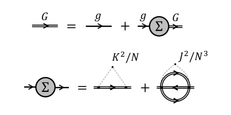
Figure 6: Self consistent relations for a Thouless pump with SYK interactions. Single lines represent the non-interacting Green’s function $g_{ss^{\prime}}(k;t,t^{\prime})$. Double lines represent the renormalized Green’s functions $G_{ss^{\prime}}(k;t,t^{\prime})$.

Appendix E Details of the numerical simulation

Here, we present the details of the numerical simulation of the time-evolution of the Kadanoff-Baym equations [see Eq. (3)]. The time-evolution is performed with respect to the SYK Hamiltonian, given in Eq. (2), with $N\to\infty$. To stabilize the numerics in the weakly-interacting limit, we added a weak random quadratic term

$$\hat{\mathcal{H}}_{\rm SYK-2}=\sum_{j,{\alpha}{\beta}}K_{{\alpha}{\beta}}\hat{c}_{j{\alpha}}^{\dagger}\hat{c}_{j{\beta}}+{\rm h.c.},$$ (32)

where $\overline{K_{{\alpha}{\beta}}}=0$ and $\overline{K_{{\alpha}{\beta}}^{2}}=K^{2}/N$.

Instead of evolving in time the $G^{R}$ and $G^{<}$ functions, as appears in Eq. (3), we found it more convenient to evolve the retarded $G^{R}$, and Keldysh components $G^{K}$. The latter is defined as

$$G_{ss^{\prime}}^{K}(k;t,t^{\prime})=G_{ss^{\prime}}^{>}(k;t,t^{\prime})+G_{ss^{\prime}}^{<}(k;t,t^{\prime}).$$ (33)

The Kadanoff-Baym equations for these two components read

$$[i\partial_{t}-H_{0}(t)]G^{R}={\delta}(t-t^{\prime})+{\Sigma}^{R}\circ G^{R}$$ (34a)

$$[i\partial_{t}-H_{0}(t)]G^{K}={\Sigma}^{R}\circ G^{K}+{\Sigma}^{K}\circ G^{A}.$$ (34b)

The disorder-averaged self-energy for the chain of SYK dots with SYK-4 [Eq. (2)] and SYK-2 [Eq. (32)] interactions can be written in the self-consistent form. The diagrammatic structure of the self-energy to the leading order in $N$ is shown in Fig. 6 Maldacena and Stanford (2016). As follows from this diagram, the greater and lesser components of the self-energy are given by

$$\begin{split}{\Sigma}^{\gtrless}_{ss^{\prime}}(x;t,t^{\prime})=&K^{2}G^{\gtrless}_{ss^{\prime}}(x;t,t^{\prime})+\\ +&J^{2}[G^{\gtrless}_{ss^{\prime}}(x;t,t^{\prime})]^{2}G_{s^{\prime}s}^{\lessgtr}(-x;t^{\prime},t).\end{split}$$ (35)

Here, $x$ is obtained from the Fourier transform of the momentum, $k$, index. The retarded and Keldysh Green’s functions $G^{R}$ and $G^{K}$ [appearing in Eq. (34)], are related to $G^{\gtrless}$ via $G^{R}_{ss^{\prime}}(k;t,t^{\prime})={\theta}(t-t^{\prime})[G_{ss^{\prime}}^{>}(k;t,t^{\prime})-G_{ss^{\prime}}^{<}(k;t,t^{\prime})]$ and Eq. (33). In turn, the inverse relatons read $G^{\gtrless}={\frac{1}{2}}\left[G^{K}\pm(G^{R}-G^{A})\right]$, where $G^{A}_{ss^{\prime}}(k;t,t^{\prime})=G^{R}_{s^{\prime}s}(k;t^{\prime},t)^{\dagger}$. The relations for the self energy are similar, with $G$ replaced by ${\Sigma}$.

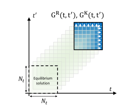
Figure 7: Time evolution of the retarded and Keldysh Green’s functions according to the Kadanoff-Baym equations [Eqs. (34)]. The square in the bottom left corner represents the initial conditions for the Green’s function, $G_{\rm eq}(t,t^{\prime})$. At each step of the evolution a new row, column and a cell on the diagonal are added to the matrix, corresponding to $G(t_{0}+{\delta}t,t)$, $G(t,t_{0}+{\delta}t)$ and $G(t_{0}+{\delta}t,t_{0}+{\delta}t)$.

E.1 Equilibrium solution

Equations (34) and (35) constitute a set of integro-differential equations which determine the time evolution of the Green’s functions. Initial conditions for this time-evolution are set by the state ${\rho}_{0}$, corresponding to equilibrium with an inverse temperature ${\beta}_{0}$ and Hamiltonian $\hat{\mathcal{H}}(0)$. Due to invariance to time-translations in equilibrium, the equilibrium Green’s functions depend only on the time-difference ${\Delta}t=t-t^{\prime}$. To find the equilibrium solution, we we evaluate Eq. (34a) for $H_{0}(t)$ at $t=0$ and transform ${\Delta}t$ to the frequency space ${\omega}$, giving rise to

$$[{\omega}-H_{0}(0)]G^{R}({\omega})=1+{\Sigma}^{R}({\omega})G^{R}({\omega}).$$ (36)

Furthermore, Eq. (34b) is trivially satisfied in equilibrium, due to the fluctuation-dissipation theorem Chaikin and Lubensky (1995); Rammer (2007); Kamenev (2011),

$$G^{K}_{ss^{\prime}}({\omega})=F({\omega})[G^{R}_{ss^{\prime}}({\omega})-G^{A}_{ss^{\prime}}({\omega})],$$ (37)

where $F({\omega})=\tanh({\beta}_{0}{\omega}/2)$. The equilibrium Green’s function is obtained from the self-consistent solution of Eqs. (35), (36) and (37).

E.2 Time evolution

Having found an equilibrium solution, $G^{R}_{\rm eq}(k;t-t^{\prime})$ and $G^{K}_{\rm eq}(k;t-t^{\prime})$, we rearrange the vectors into matrices $[G_{\rm eq}^{R}]_{ss^{\prime}}(k;t,t^{\prime})$ and $[G^{K}_{\rm eq}]_{ss^{\prime}}(k;t,t^{\prime})$ of size $N_{t}\times N_{t}$ in the time domain and $2\times 2$ in the sublattice space, for a vector of crystal momenta of size $L$. In our simulations, we used $N_{t}=3000$ (smaller values of $N_{t}$ are used to vary ${\delta}{\omega}$ and ${\delta}t$), and $L=50$. We used the equilibrium solution as the starting point of the simulation to propagate the Green’s functions by one time step ${\delta}t$ in each iteration according to Eq. (34) Stan et al. (2009), see Fig. 7. In particular, given $G^{R}(t_{0},t^{\prime})$, we evolve $G^{R}$ according to:

$$\begin{split}&G^{R}(t_{0}+{\delta}t,t^{\prime})=U_{0}(t_{0})[G^{R}(t_{0},t^{\prime})-\frac{i}{2}{\delta}_{t,t^{\prime}}]-i{\delta}tI^{R}(t^{\prime})\end{split}$$ (38)

for $t^{\prime}\leq t_{0}$; $G^{R}(t,t_{0}+{\delta}t)=0$ for $t\leq t_{0}$; and $G^{R}(t_{0}+{\delta}t,t_{0}+{\delta}t)=G^{R}(t_{0},t_{0})$. Here we defined $U_{0}(t)=e^{-i{\delta}tH_{0}(t)}$ and $I^{R}(t^{\prime})=\int{\Sigma}^{R}(t_{0},s)G^{R}(s,t^{\prime})ds$.

To optimize the efficiency of the simulation, we keep the overall size of the matrices constants. Therefore, for each new element of the Green’s function calculated in the future, we erase one element in the past. Such a truncation of the Green’s function fixes the required memory of the simulation and significantly reduces the computational resources used.

References

- Oka and Aoki (2009) Takashi Oka and Hideo Aoki, “Photovoltaic Hall effect in graphene,” Phys. Rev. B 79, 081406 (2009).
- Kitagawa et al. (2010) Takuya Kitagawa, Erez Berg, Mark Rudner, and Eugene Demler, “Topological characterization of periodically driven quantum systems,” Phys. Rev. B 82, 235114 (2010).
- Lindner et al. (2011) Netanel H. Lindner, Gil Refael, and Victor Galitski, “Floquet topological insulator in semiconductor quantum wells,” Nat. Phys. 7, 490–495 (2011).
- Dalibard et al. (2011) Jean Dalibard, Fabrice Gerbier, Gediminas Juzeliunas, and Patrik Öhberg, “Colloquium: Artificial gauge potentials for neutral atoms,” Rev. Mod. Phys. 83, 1523–1543 (2011).
- Gómez-León and Platero (2013) A. Gómez-León and G. Platero, “Floquet-Bloch Theory and Topology in Periodically Driven Lattices,” Phys. Rev. Lett. 110, 200403 (2013).
- Huse et al. (2013) David A. Huse, Rahul Nandkishore, Vadim Oganesyan, Arijeet Pal, and S. L. Sondhi, “Localization-protected quantum order,” Phys. Rev. B 88, 014206 (2013).
- Rudner et al. (2013) Mark S. Rudner, Netanel H. Lindner, Erez Berg, and Michael Levin, “Anomalous edge states and the bulk-edge correspondence for periodically driven two-dimensional systems,” Phys. Rev. X 3, 031005 (2013).
- Dehghani et al. (2014) Hossein Dehghani, Takashi Oka, and Aditi Mitra, “Dissipative Floquet topological systems,” Phys. Rev. B 90, 195429 (2014).
- Foa Torres et al. (2014) L. E.F. Foa Torres, P. M. Perez-Piskunow, C. A. Balseiro, and Gonzalo Usaj, “Multiterminal conductance of a floquet topological insulator,” Phys. Rev. Lett. 113, 266801 (2014).
- Usaj et al. (2014) Gonzalo Usaj, P. M. Perez-Piskunow, L. E.F. Foa Torres, and C. A. Balseiro, “Irradiated graphene as a tunable Floquet topological insulator,” Phys. Rev. B 90, 115423 (2014).
- Chandran et al. (2014) Anushya Chandran, Vedika Khemani, C. R. Laumann, and S. L. Sondhi, “Many-body localization and symmetry-protected topological order,” Phys. Rev. B 89, 144201 (2014).
- Goldman et al. (2014) N. Goldman, G. Juzeliunas, P. Öhberg, and I. B. Spielman, “Light-induced gauge fields for ultracold atoms,” Reports Prog. Phys. 77, 126401 (2014).
- Grushin et al. (2014) Adolfo G. Grushin, Álvaro Gómez-León, and Titus Neupert, “Floquet fractional chern insulators,” Phys. Rev. Lett. 112, 156801 (2014).
- Perez-Piskunow et al. (2015) P. M. Perez-Piskunow, L. E.F. Foa Torres, and Gonzalo Usaj, “Hierarchy of Floquet gaps and edge states for driven honeycomb lattices,” Phys. Rev. A 91, 043625 (2015).
- Dal Lago et al. (2015) V. Dal Lago, M. Atala, and L. E.F. Foa Torres, “Floquet topological transitions in a driven one-dimensional topological insulator,” Phys. Rev. A 92, 023624 (2015).
- Nathan and Rudner (2015) Frederik Nathan and Mark S. Rudner, “Topological singularities and the general classification of Floquet–Bloch systems,” New J. Phys. 17, 125014 (2015).
- Khemani et al. (2016) Vedika Khemani, Achilleas Lazarides, Roderich Moessner, and S. L. Sondhi, “Phase Structure of Driven Quantum Systems,” Phys. Rev. Lett. 116, 250401 (2016).
- Von Keyserlingk and Sondhi (2016a) C. W. Von Keyserlingk and S. L. Sondhi, “Phase structure of one-dimensional interacting Floquet systems. II. Symmetry-broken phases,” Phys. Rev. B 93, 245146 (2016a).
- Von Keyserlingk and Sondhi (2016b) C. W. Von Keyserlingk and S. L. Sondhi, “Phase structure of one-dimensional interacting Floquet systems. I. Abelian symmetry-protected topological phases,” Phys. Rev. B 93, 245145 (2016b).
- Else and Nayak (2016) Dominic V. Else and Chetan Nayak, “Classification of topological phases in periodically driven interacting systems,” Phys. Rev. B 93, 201103 (2016).
- Po et al. (2016) Hoi Chun Po, Lukasz Fidkowski, Takahiro Morimoto, Andrew C. Potter, and Ashvin Vishwanath, “Chiral floquet phases of many-body localized bosons,” Phys. Rev. X 6, 041070 (2016).
- Potter et al. (2016) Andrew C. Potter, Takahiro Morimoto, and Ashvin Vishwanath, “Classification of interacting topological Floquet phases in one dimension,” Phys. Rev. X 6, 041001 (2016).
- Eckardt (2017) André Eckardt, “Colloquium: Atomic quantum gases in periodically driven optical lattices,” Rev. Mod. Phys. 89, 011004 (2017).
- Roy and Harper (2017a) Rahul Roy and Fenner Harper, “Periodic table for Floquet topological insulators,” Phys. Rev. B 96, 155118 (2017a).
- Roy and Harper (2017b) Rahul Roy and Fenner Harper, “Floquet topological phases with symmetry in all dimensions,” Phys. Rev. B 95, 195128 (2017b).
- Harper and Roy (2017) Fenner Harper and Rahul Roy, “Floquet Topological Order in Interacting Systems of Bosons and Fermions,” Phys. Rev. Lett. 118, 115301 (2017).
- Gong et al. (2018) Zongping Gong, Yuto Ashida, Kohei Kawabata, Kazuaki Takasan, Sho Higashikawa, and Masahito Ueda, “Topological Phases of Non-Hermitian Systems,” Phys. Rev. X 8, 031079 (2018).
- Esin et al. (2018) Iliya Esin, Mark S. Rudner, Gil Refael, and Netanel H. Lindner, “Quantized transport and steady states of Floquet topological insulators,” Phys. Rev. B 97, 245401 (2018).
- Ozawa et al. (2019) Tomoki Ozawa, Hannah M. Price, Alberto Amo, Nathan Goldman, Mohammad Hafezi, Ling Lu, Mikael C. Rechtsman, David Schuster, Jonathan Simon, Oded Zilberberg, and Iacopo Carusotto, “Topological photonics,” Rev. Mod. Phys. 91, 015006 (2019).
- Cooper et al. (2019) N. R. Cooper, J. Dalibard, and I. B. Spielman, “Topological bands for ultracold atoms,” Rev. Mod. Phys. 91, 015005 (2019).
- Rudner and Lindner (2020a) Mark S. Rudner and Netanel H. Lindner, “Band structure engineering and non-equilibrium dynamics in Floquet topological insulators,” Nat. Rev. Phys. 2, 229–244 (2020a).
- Harper et al. (2020) Fenner Harper, Rahul Roy, Mark S. Rudner, and S. L. Sondhi, “Topology and Broken Symmetry in Floquet Systems,” Annu. Rev. Condens. Matter Phys. 11, 345–368 (2020).
- Zhang and Yang (2021) Rui Xing Zhang and Zhi Cheng Yang, “Tunable fragile topology in Floquet systems,” Phys. Rev. B 103, L121115 (2021).
- Arovas et al. (1985) Daniel P. Arovas, Robert Schrieffer, Frank Wilczek, and A. Zee, “Statistical mechanics of anyons,” Nucl. Phys. B 251, 117–126 (1985).
- Altland and Zirnbauer (1997) Alexander Altland and Martin R. Zirnbauer, “Nonstandard symmetry classes in mesoscopic normal-superconducting hybrid structures,” Phys. Rev. B 55, 1142 (1997).
- Kitaev (2006) Alexei Kitaev, “Anyons in an exactly solved model and beyond,” Ann. Phys. (N. Y). 321, 2–111 (2006).
- Stern (2008) Ady Stern, “Anyons and the quantum Hall effect—A pedagogical review,” Ann. Phys. (N. Y). 323, 204–249 (2008).
- Nayak et al. (2008) Chetan Nayak, Steven H. Simon, Ady Stern, Michael Freedman, and Sankar Das Sarma, “Non-Abelian anyons and topological quantum computation,” Rev. Mod. Phys. 80, 1083–1159 (2008).
- Kitaev (2009) Alexei Kitaev, “Periodic table for topological insulators and superconductors,” AIP Conf. Proc. 1134, 22 (2009).
- Hasan and Kane (2010) M. Z. Hasan and C. L. Kane, “Colloquium: Topological insulators,” Rev. Mod. Phys. 82, 3045–3067 (2010).
- Qi and Zhang (2011) Xiao Liang Qi and Shou Cheng Zhang, “Topological insulators and superconductors,” Rev. Mod. Phys. 83, 1057 (2011).
- Fidkowski and Kitaev (2011) Lukasz Fidkowski and Alexei Kitaev, “Topological phases of fermions in one dimension,” Phys. Rev. B 83, 075103 (2011).
- Ren et al. (2016) Yafei Ren, Zhenhua Qiao, and Qian Niu, “Topological phases in two-dimensional materials: a review,” Reports Prog. Phys. 79, 066501 (2016).
- Chiu et al. (2016) Ching Kai Chiu, Jeffrey C.Y. Teo, Andreas P. Schnyder, and Shinsei Ryu, “Classification of topological quantum matter with symmetries,” Rev. Mod. Phys. 88, 035005 (2016).
- Wen (2017) Xiao Gang Wen, “Colloquium: Zoo of quantum-topological phases of matter,” Rev. Mod. Phys. 89, 041004 (2017).
- Aidelsburger et al. (2011) M. Aidelsburger, M. Atala, S. Nascimbène, S. Trotzky, Y. A. Chen, and I. Bloch, “Experimental realization of strong effective magnetic fields in an optical lattice,” Phys. Rev. Lett. 107, 255301 (2011).
- Rechtsman et al. (2013) Mikael C. Rechtsman, Julia M. Zeuner, Yonatan Plotnik, Yaakov Lumer, Daniel Podolsky, Felix Dreisow, Stefan Nolte, Mordechai Segev, and Alexander Szameit, “Photonic Floquet topological insulators,” Nature 496, 196–200 (2013).
- Aidelsburger et al. (2014) M. Aidelsburger, M. Lohse, C. Schweizer, M. Atala, J. T. Barreiro, S. Nascimbène, N. R. Cooper, I. Bloch, and N. Goldman, “Measuring the Chern number of Hofstadter bands with ultracold bosonic atoms,” Nat. Phys. 11, 162–166 (2014).
- Jotzu et al. (2014) Gregor Jotzu, Michael Messer, Rémi Desbuquois, Martin Lebrat, Thomas Uehlinger, Daniel Greif, and Tilman Esslinger, “Experimental realization of the topological Haldane model with ultracold fermions,” Nature 515, 237–240 (2014).
- Fleury et al. (2016) Romain Fleury, Alexander B. Khanikaev, and Andrea Alù, “Floquet topological insulators for sound,” Nat. Commun. 7, 1–11 (2016).
- Basov et al. (2017) D. N. Basov, R. D. Averitt, and D. Hsieh, “Towards properties on demand in quantum materials,” Nat. Mater. 16, 1077–1088 (2017).
- Oka and Kitamura (2019) Takashi Oka and Sota Kitamura, “Floquet Engineering of Quantum Materials,” Annu. Rev. Condens. Matter Phys. 10, 387–408 (2019).
- McIver et al. (2019) J. W. McIver, B. Schulte, F. U. Stein, T. Matsuyama, G. Jotzu, G. Meier, and A. Cavalleri, “Light-induced anomalous Hall effect in graphene,” Nat. Phys. 16, 38–41 (2019).
- Shan et al. (2021) Jun-Yi Shan, M. Ye, H. Chu, Sungmin Lee, Je-Geun Park, L. Balents, and D. Hsieh, “Giant modulation of optical nonlinearity by Floquet engineering,” Nature 600, 235–239 (2021).
- Mukherjee and Rechtsman (2021) Sebabrata Mukherjee and Mikael C. Rechtsman, “Observation of Unidirectional Solitonlike Edge States in Nonlinear Floquet Topological Insulators,” Phys. Rev. X 11, 041057 (2021).
- Else et al. (2016) Dominic V. Else, Bela Bauer, and Chetan Nayak, “Floquet Time Crystals,” Phys. Rev. Lett. 117, 090402 (2016).
- Titum et al. (2016) Paraj Titum, Erez Berg, Mark S. Rudner, Gil Refael, and Netanel H. Lindner, “Anomalous Floquet-Anderson Insulator as a nonadiabatic quantized charge pump,” Phys. Rev. X 6, 021013 (2016).
- Peng et al. (2016) Yu Gui Peng, Cheng Zhi Qin, De Gang Zhao, Ya Xi Shen, Xiang Yuan Xu, Ming Bao, Han Jia, and Xue Feng Zhu, “Experimental demonstration of anomalous Floquet topological insulator for sound,” Nat. Commun. 7, 1–8 (2016).
- Zhang et al. (2017) J. Zhang, P. W. Hess, A. Kyprianidis, P. Becker, A. Lee, J. Smith, G. Pagano, I. D. Potirniche, A. C. Potter, A. Vishwanath, N. Y. Yao, and C. Monroe, “Observation of a discrete time crystal,” Nature 543, 217–220 (2017).
- Choi et al. (2017) Soonwon Choi, Joonhee Choi, Renate Landig, Georg Kucsko, Hengyun Zhou, Junichi Isoya, Fedor Jelezko, Shinobu Onoda, Hitoshi Sumiya, Vedika Khemani, Curt Von Keyserlingk, Norman Y. Yao, Eugene Demler, and Mikhail D. Lukin, “Observation of discrete time-crystalline order in a disordered dipolar many-body system,” Nature 543, 221–225 (2017).
- Maczewsky et al. (2017) Lukas J. Maczewsky, Julia M. Zeuner, Stefan Nolte, and Alexander Szameit, “Observation of photonic anomalous Floquet topological insulators,” Nat. Commun. 8, 1–7 (2017).
- Mukherjee et al. (2017) Sebabrata Mukherjee, Alexander Spracklen, Manuel Valiente, Erika Andersson, Patrik Öhberg, Nathan Goldman, and Robert R. Thomson, “Experimental observation of anomalous topological edge modes in a slowly driven photonic lattice,” Nat. Commun. 8, 1–7 (2017).
- Nathan et al. (2019) Frederik Nathan, Dmitry Abanin, Erez Berg, Netanel H. Lindner, and Mark S. Rudner, “Anomalous Floquet insulators,” Phys. Rev. B 99, 195133 (2019).
- Wintersperger et al. (2020) Karen Wintersperger, Christoph Braun, F. Nur Ünal, André Eckardt, Marco Di Liberto, Nathan Goldman, Immanuel Bloch, and Monika Aidelsburger, “Realization of an anomalous Floquet topological system with ultracold atoms,” Nat. Phys. 16, 1058–1063 (2020).
- Afzal et al. (2020) Shirin Afzal, Tyler J. Zimmerling, Yang Ren, David Perron, and Vien Van, “Realization of Anomalous Floquet Insulators in Strongly Coupled Nanophotonic Lattices,” Phys. Rev. Lett. 124, 253601 (2020).
- Esin et al. (2020) Iliya Esin, Mark S. Rudner, and Netanel H. Lindner, “Floquet metal-to-insulator phase transitions in semiconductor nanowires,” Sci. Adv. 6, eaay4922 (2020).
- Esin et al. (2021) Iliya Esin, Gaurav Kumar Gupta, Erez Berg, Mark S. Rudner, and Netanel H. Lindner, “Electronic Floquet gyro-liquid crystal,” Nat. Commun. 12, 1–12 (2021).
- Thouless (1983) D. J. Thouless, “Quantization of particle transport,” Phys. Rev. B 27, 6083–6087 (1983).
- Niu and Thouless (1984) Q Niu and D J Thouless, “Quantised adiabatic charge transport in the presence of substrate disorder and many-body interaction,” J. Phys. A 17, 2453 (1984).
- Niu (1990) Q. Niu, “Towards a quantum pump of electric charges,” Phys. Rev. Lett. 64, 1812 (1990).
- Brouwer (1998) P. Brouwer, “Scattering approach to parametric pumping,” Phys. Rev. B 58, R10135 (1998).
- Switkes (1999) M. Switkes, “An adiabatic quantum electron pump,” Science 283, 1905–1908 (1999).
- Altshuler and Glazman (1999) B. L. Altshuler and L. I. Glazman, “Pumping electrons,” Science 283, 1864–1865 (1999).
- Chern et al. (2007) Chyh Hong Chern, Shigeki Onoda, Shuichi Murakami, and Naoto Nagaosa, “Quantum charge pumping and electric polarization in Anderson insulators,” Phys. Rev. B 76, 035334 (2007).
- Xiao et al. (2010) Di Xiao, Ming Che Chang, and Qian Niu, “Berry phase effects on electronic properties,” Rev. Mod. Phys. 82, 1959–2007 (2010).
- Meidan et al. (2011) Dganit Meidan, Tobias Micklitz, and Piet W. Brouwer, “Topological classification of adiabatic processes,” Phys. Rev. B 84, 195410 (2011).
- Wang et al. (2013) Y. H. Wang, H. Steinberg, P. Jarillo-Herrero, and N. Gedik, “Observation of floquet-bloch states on the surface of a topological insulator,” Science 342, 453–457 (2013).
- Keller et al. (1999) Mark W. Keller, Ali L. Eichenberger, John M. Martinis, and Neil M. Zimmerman, “A capacitance standard based on counting electrons,” Science 285, 1706–1709 (1999).
- Piquemal et al. (2004) François Piquemal, Alexandre Bounouh, Laurent Devoille, Nicolas Feltin, Olivier Thevenot, and Gérard Trapon, “Fundamental electrical standards and the quantum metrological triangle,” Comptes Rendus Phys. 5, 857–879 (2004).
- Blumenthal et al. (2007) M. D. Blumenthal, B. Kaestner, L. Li, S. Giblin, T. J.B.M. Janssen, M. Pepper, D. Anderson, G. Jones, and D. A. Ritchie, “Gigahertz quantized charge pumping,” Nat. Phys. 3, 343–347 (2007).
- Giblin et al. (2012) S. P. Giblin, M. Kataoka, J. D. Fletcher, P. See, T. J.B.M. Janssen, J. P. Griffiths, G. A.C. Jones, I. Farrer, and D. A. Ritchie, “Towards a quantum representation of the ampere using single electron pumps,” Nat. Commun. 3, 1–6 (2012).
- Pekola et al. (2013) Jukka P. Pekola, Olli Pentti Saira, Ville F. Maisi, Antti Kemppinen, Mikko Möttönen, Yuri A. Pashkin, and Dmitri V. Averin, “Single-electron current sources: Toward a refined definition of the ampere,” Rev. Mod. Phys. 85, 1421–1472 (2013).
- Fletcher et al. (2013) J. D. Fletcher, P. See, H. Howe, M. Pepper, S. P. Giblin, J. P. Griffiths, G. A.C. Jones, I. Farrer, D. A. Ritchie, T. J.B.M. Janssen, and M. Kataoka, “Clock-controlled emission of single-electron wave packets in a solid-state circuit,” Phys. Rev. Lett. 111, 216807 (2013).
- Ubbelohde et al. (2014) Niels Ubbelohde, Frank Hohls, Vyacheslavs Kashcheyevs, Timo Wagner, Lukas Fricke, Bernd Kästner, Klaus Pierz, Hans W. Schumacher, and Rolf J. Haug, “Partitioning of on-demand electron pairs,” Nat. Nanotechnol. 10, 46–49 (2014).
- Johnson et al. (2017) N. Johnson, J. D. Fletcher, D. A. Humphreys, P. See, J. P. Griffiths, G. A.C. Jones, I. Farrer, D. A. Ritchie, M. Pepper, T. J.B.M. Janssen, and M. Kataoka, “Ultrafast voltage sampling using single-electron wavepackets,” Appl. Phys. Lett. 110, 102105 (2017).
- Kraus et al. (2012) Yaacov E. Kraus, Yoav Lahini, Zohar Ringel, Mor Verbin, and Oded Zilberberg, “Topological states and adiabatic pumping in quasicrystals,” Phys. Rev. Lett. 109, 106402 (2012).
- Schweizer et al. (2016) C. Schweizer, M. Lohse, R. Citro, and I. Bloch, “Spin Pumping and Measurement of Spin Currents in Optical Superlattices,” Phys. Rev. Lett. 117, 170405 (2016).
- Lohse et al. (2016) M. Lohse, C. Schweizer, O. Zilberberg, M. Aidelsburger, and I. Bloch, “A Thouless quantum pump with ultracold bosonic atoms in an optical superlattice,” Nat. Phys. 12, 350–354 (2016).
- Nakajima et al. (2016) Shuta Nakajima, Takafumi Tomita, Shintaro Taie, Tomohiro Ichinose, Hideki Ozawa, Lei Wang, Matthias Troyer, and Yoshiro Takahashi, “Topological Thouless pumping of ultracold fermions,” Nat. Phys. 12, 296–300 (2016).
- Zilberberg et al. (2018) Oded Zilberberg, Sheng Huang, Jonathan Guglielmon, Mohan Wang, Kevin P. Chen, Yaacov E. Kraus, and Mikael C. Rechtsman, “Photonic topological boundary pumping as a probe of 4D quantum Hall physics,” Nature 553, 59–62 (2018).
- Lohse et al. (2018) Michael Lohse, Christian Schweizer, Hannah M. Price, Oded Zilberberg, and Immanuel Bloch, “Exploring 4D quantum Hall physics with a 2D topological charge pump,” Nature 553, 55–58 (2018).
- Cerjan et al. (2020) Alexander Cerjan, Mohan Wang, Sheng Huang, Kevin P. Chen, and Mikael C. Rechtsman, “Thouless pumping in disordered photonic systems,” Light Sci. Appl. 9, 1–7 (2020).
- Nakajima et al. (2021) Shuta Nakajima, Nobuyuki Takei, Keita Sakuma, Yoshihito Kuno, Pasquale Marra, and Yoshiro Takahashi, “Competition and interplay between topology and quasi-periodic disorder in Thouless pumping of ultracold atoms,” Nat. Phys. 17, 844–849 (2021).
- Jürgensen et al. (2021) Marius Jürgensen, Sebabrata Mukherjee, and Mikael C. Rechtsman, “Quantized nonlinear Thouless pumping,” Nature 596, 63–67 (2021).
- Minguzzi et al. (2021) Joaquín Minguzzi, Zijie Zhu, Kilian Sandholzer, Anne-Sophie Walter, Konrad Viebahn, and Tilman Esslinger, “Topological pumping in a Floquet-Bloch band,” (2021), arXiv:2112.12788 .
- Lazarides et al. (2014) Achilleas Lazarides, Arnab Das, and Roderich Moessner, “Equilibrium states of generic quantum systems subject to periodic driving,” Phys. Rev. E 90, 012110 (2014).
- D’Alessio and Rigol (2014) Luca D’Alessio and Marcos Rigol, “Long-time behavior of isolated periodically driven interacting lattice systems,” Phys. Rev. X 4, 041048 (2014).
- Ponte et al. (2015) Pedro Ponte, Anushya Chandran, Z. Papić, and Dmitry A. Abanin, “Periodically driven ergodic and many-body localized quantum systems,” Ann. Phys. (N. Y). 353, 196–204 (2015).
- Bukov et al. (2015) Marin Bukov, Luca D’Alessio, and Anatoli Polkovnikov, “Universal high-frequency behavior of periodically driven systems: from dynamical stabilization to Floquet engineering,” Adv. Phys. 64, 139–226 (2015).
- Eckardt and Anisimovas (2015) André Eckardt and Egidijus Anisimovas, “High-frequency approximation for periodically driven quantum systems from a Floquet-space perspective,” New J. Phys. 17, 093039 (2015).
- Abanin et al. (2015) Dmitry A. Abanin, Wojciech De Roeck, and François Huveneers, “Exponentially Slow Heating in Periodically Driven Many-Body Systems,” Phys. Rev. Lett. 115, 256803 (2015).
- Bukov et al. (2016) Marin Bukov, Markus Heyl, David A. Huse, and Anatoli Polkovnikov, “Heating and many-body resonances in a periodically driven two-band system,” Phys. Rev. B 93, 155132 (2016).
- Kuwahara et al. (2016) Tomotaka Kuwahara, Takashi Mori, and Keiji Saito, “Floquet–Magnus theory and generic transient dynamics in periodically driven many-body quantum systems,” Ann. Phys. (N. Y). 367, 96–124 (2016).
- Else et al. (2017) Dominic V. Else, Bela Bauer, and Chetan Nayak, “Prethermal phases of matter protected by time-translation symmetry,” Phys. Rev. X 7, 011026 (2017).
- Abanin et al. (2017) Dmitry Abanin, Wojciech De Roeck, Wen Wei Ho, and François Huveneers, “A Rigorous Theory of Many-Body Prethermalization for Periodically Driven and Closed Quantum Systems,” Commun. Math. Phys. 354, 809–827 (2017).
- Reitter et al. (2017) Martin Reitter, Jakob Näger, Karen Wintersperger, Christoph Sträter, Immanuel Bloch, André Eckardt, and Ulrich Schneider, “Interaction Dependent Heating and Atom Loss in a Periodically Driven Optical Lattice,” Phys. Rev. Lett. 119, 200402 (2017).
- Mori (2018) Takashi Mori, “Floquet prethermalization in periodically driven classical spin systems,” Phys. Rev. B 98, 104303 (2018).
- Howell et al. (2019) Owen Howell, Phillip Weinberg, Dries Sels, Anatoli Polkovnikov, and Marin Bukov, “Asymptotic Prethermalization in Periodically Driven Classical Spin Chains,” Phys. Rev. Lett. 122, 010602 (2019).
- Vogl et al. (2019) Michael Vogl, Pontus Laurell, Aaron D. Barr, and Gregory A. Fiete, “Flow Equation Approach to Periodically Driven Quantum Systems,” Phys. Rev. X 9, 021037 (2019).
- Kuhlenkamp and Knap (2020) Clemens Kuhlenkamp and Michael Knap, “Periodically Driven Sachdev-Ye-Kitaev Models,” Phys. Rev. Lett. 124, 106401 (2020).
- Fleckenstein and Bukov (2021) Christoph Fleckenstein and Marin Bukov, “Thermalization and prethermalization in periodically kicked quantum spin chains,” Phys. Rev. B 103, 144307 (2021).
- Lindner et al. (2017) Netanel H. Lindner, Erez Berg, and Mark S. Rudner, “Universal chiral quasisteady states in periodically driven many-body systems,” Phys. Rev. X 7, 011018 (2017).
- Gulden et al. (2020) Tobias Gulden, Mark S Rudner, Erez Berg, and Netanel H Lindner, “Exponentially long lifetime of universal quasi-steady states in topological Floquet pumps,” SciPost Phys 9, 15 (2020).
- Gawatz et al. (2021) Raffael Gawatz, Ajit C. Balram, Erez Berg, Netanel H. Lindner, and Mark S. Rudner, “Prethermalization and entanglement dynamics in interacting topological pumps,” (2021), arXiv:2103.15831 .
- Sachdev and Ye (1993) Subir Sachdev and Jinwu Ye, “Gapless spin-fluid ground state in a random quantum Heisenberg magnet,” Phys. Rev. Lett. 70, 3339–3342 (1993).
- (116) A. Kitaev, ““A simple model of quantum holography.” http://online.kitp.ucsb.edu/online/entangled15/kitaev/,http: //online.kitp.ucsb.edu/online/entangled15/kitaev2/. Talks at KITP, April 7, 2015 and May 27, 2015,” .
- Maldacena and Stanford (2016) Juan Maldacena and Douglas Stanford, “Remarks on the Sachdev-Ye-Kitaev model,” Phys. Rev. D 94, 106002 (2016).
- White and Feiguin (2004) Steven R. White and Adrian E. Feiguin, “Real-time evolution using the density matrix renormalization group,” Phys. Rev. Lett. 93, 076401 (2004).
- Schollwöck (2005) U. Schollwöck, “The density-matrix renormalization group,” Rev. Mod. Phys. 77, 259–315 (2005).
- Rice and Mele (1982) M. J. Rice and E. J. Mele, “Elementary excitations of a linearly conjugated diatomic polymer,” Phys. Rev. Lett. 49, 1455–1459 (1982).
- Chowdhury et al. (2018) Debanjan Chowdhury, Yochai Werman, Erez Berg, and T. Senthil, “Translationally Invariant Non-Fermi-Liquid Metals with Critical Fermi Surfaces: Solvable Models,” Phys. Rev. X 8, 031024 (2018).
- Patel et al. (2018) Aavishkar A. Patel, John McGreevy, Daniel P. Arovas, and Subir Sachdev, “Magnetotransport in a Model of a Disordered Strange Metal,” Phys. Rev. X 8, 021049 (2018).
- Shih and Niu (1994) Wei Kai Shih and Qian Niu, “Nonadiabatic particle transport in a one-dimensional electron system,” Phys. Rev. B 50, 11902 (1994).
- Privitera et al. (2018) Lorenzo Privitera, Angelo Russomanno, Roberta Citro, and Giuseppe E. Santoro, “Nonadiabatic Breaking of Topological Pumping,” Phys. Rev. Lett. 120, 106601 (2018).
- Rudner and Lindner (2020b) Mark S. Rudner and Netanel H. Lindner, “The Floquet Engineer’s Handbook,” (2020b), arXiv:2003.08252 .
- Shirley (1965) Jon H. Shirley, “Solution of the Schrödinger Equation with a Hamiltonian Periodic in Time,” Phys. Rev. 138, B979 (1965).
- Sambe (1973) Hideo Sambe, “Steady States and Quasienergies of a Quantum-Mechanical System in an Oscillating Field,” Phys. Rev. A 7, 2203 (1973).
- Baym and Kadanoff (1962) Gordon Baym and Leo P. Kadanoff, Quantum Statistical Mechanics (Benjamin, New York, 1962).
- Rammer and Smith (1986) J. Rammer and H. Smith, “Quantum field-theoretical methods in transport theory of metals,” Rev. Mod. Phys. 58, 323 (1986).
- Rammer (2007) Jørgen. Rammer, Quantum field theory of non-equilibrium states (Cambridge University Press, 2007) p. 536.
- Kamenev (2011) Alex Kamenev, Field Theory of Non-Equilibrium Systems (2011).
- Picano et al. (2021) Antonio Picano, Jiajun Li, and Martin Eckstein, “Quantum Boltzmann equation for strongly correlated electrons,” Phys. Rev. B 104, 085108 (2021).
- Genske and Rosch (2015) Maximilian Genske and Achim Rosch, “Floquet-Boltzmann equation for periodically driven Fermi systems,” Phys. Rev. A 92, 062108 (2015).
- Stan et al. (2009) Adrian Stan, Nils Erik Dahlen, and Robert Van Leeuwen, “Time propagation of the Kadanoff-Baym equations for inhomogeneous systems,” J. Chem. Phys. 130, 224101 (2009).
- Eberlein et al. (2017) Andreas Eberlein, Valentin Kasper, Subir Sachdev, and Julia Steinberg, “Quantum quench of the Sachdev-Ye-Kitaev model,” Phys. Rev. B 96, 205123 (2017).
- Bhattacharya et al. (2019) Ritabrata Bhattacharya, Dileep P. Jatkar, and Nilakash Sorokhaibam, “Quantum quenches and thermalization in SYK models,” J. High Energy Phys. 2019, 66 (2019).
- Maldacena and Milekhin (2021) Juan Maldacena and Alexey Milekhin, “SYK wormhole formation in real time,” J. High Energy Phys. 2021, 1–40 (2021).
- Kitagawa et al. (2011) Takuya Kitagawa, Takashi Oka, Arne Brataas, Liang Fu, and Eugene Demler, “Transport properties of nonequilibrium systems under the application of light: Photoinduced quantum Hall insulators without Landau levels,” Phys. Rev. B 84, 235108 (2011).
- Chaikin and Lubensky (1995) P. M. Chaikin and T. C. Lubensky, Princ. Condens. Matter Phys. (Cambridge University Press, 1995).