Evolving Curricula with Regret-Based Environment Design

Abstract

Training generally-capable agents with reinforcement learning (RL) remains a significant challenge. A promising avenue for improving the robustness of RL agents is through the use of curricula. One such class of methods frames environment design as a game between a student and a teacher, using regret-based objectives to produce environment instantiations (or levels) at the frontier of the student agent’s capabilities. These methods benefit from theoretical robustness guarantees at equilibrium, yet they often struggle to find effective levels in challenging design spaces in practice. By contrast, evolutionary approaches incrementally alter environment complexity, resulting in potentially open-ended learning, but often rely on domain-specific heuristics and vast amounts of computational resources. This work proposes harnessing the power of evolution in a principled, regret-based curriculum. Our approach, which we call Adversarially Compounding Complexity by Editing Levels (ACCEL), seeks to constantly produce levels at the frontier of an agent’s capabilities, resulting in curricula that start simple but become increasingly complex. ACCEL maintains the theoretical benefits of prior regret-based methods, while providing significant empirical gains in a diverse set of environments. An interactive version of this paper is available at https://accelagent.github.io.

1 Introduction

Reinforcement Learning (RL, Sutton and Barto, (1998)) considers the problem of an agent learning through experience to maximize reward in a given environment. The past decade has seen a surge of interest in RL, with high profile successes in games (Vinyals et al.,, 2019; Berner et al.,, 2019; Silver et al.,, 2016; Mnih et al.,, 2013; Hu and Foerster,, 2020) and robotics (OpenAI et al.,, 2019; Andrychowicz et al.,, 2020), with some believing RL may be sufficient for producing generally capable agents (Silver et al.,, 2021). Despite the promise of RL, it is often a challenge to train agents capable of systematic generalization (Kirk et al.,, 2021).

This work focuses on the use of adaptive curricula for training more generally-capable agents. By adapting the training distribution over the parameters of an environment, adaptive curricula have been shown to produce more robust policies in fewer training steps (Portelas et al.,, 2019; Jiang et al., 2021b, ). For example, these parameters may correspond to friction coefficients in a robotics simulator or maze layouts for a navigation task. Each concrete setting of parameters results in an environment instance called a level. Indeed in many prominent RL successes, adaptive curricula have played a key role, acting over opponents (Vinyals et al.,, 2019), game levels (Team et al.,, 2021), or parameters of a simulator (OpenAI et al.,, 2019; Andrychowicz et al.,, 2020).

Unsupervised Environment Design (UED, Dennis et al., (2020)) formalizes the problem of finding adaptive curricula, whereby a teacher agent designs levels using feedback from a student, which seeks to solve them. When using regret as feedback, Dennis et al., (2020) showed that if the system reaches equilibrium, then the student must follow a minimax regret strategy, i.e. the student would be capable of solving all solvable environments. This approach produces student policies exhibiting impressive zero-shot transfer to challenging human designed environments (Dennis et al.,, 2020; Jiang et al., 2021a, ; Gur et al.,, 2021). However, training such an adversarial teacher remains a challenge, and so far, the strongest empirical results come from curating randomly sampled levels for high-regret, rather than learning to directly design such levels (Jiang et al., 2021a, ). This approach is unable to take advantage of any previously discovered level structures, and its performance can be expected to degrade as the size of the design space grows.

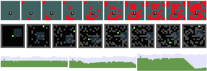
Figure 1: The evolution of a level in three different environments: MiniHack lava grids, MiniGrid mazes and BipedalWalker terrains. In each case, the far left shows a base level, acting as a parent for subsequent edited levels to the right. Each level along the evolutionary path has a high regret for the student agent at that point in time. Thus the level difficulty co-evolves with the agent’s capabilities. In each environment, we see that despite starting with simple levels, the pursuit of high regret leads to increasingly complex challenges. This complexity emerges entirely without relying on any environment-specific exploration heuristics. Note that since the agent can move diagonally in the lava environment, the final level in the top row is solvable.

An important benefit of adaptive curricula is the possibility of open-ended learning (Soros and Stanley,, 2014), given the curriculum can be steered toward constantly designing novel tasks for the agent to solve. While generating truly open-ended learning remains a grand challenge (Stanley et al.,, 2017), recent works in the evolutionary community have taken the first steps in this direction, through methods such as Minimal Criteria Coevolution (MCC, Brant and Stanley, (2017)) and POET (Wang et al.,, 2019, 2020). These approaches show that evolving levels can effectively produce agents capable of solving a diverse range of challenging tasks. In contrast to prior UED works, these evolutionary methods directly take advantage of the most useful structures found so far in a constant process of mutation and selection. However, the key drawbacks of these methods are their reliance on domain specific heuristics and need for vast computational resources, making it challenging for the community to make further progress in this direction.

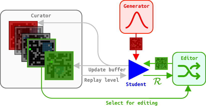
Figure 2: An overview of ACCEL. Levels are randomly sampled from a generator and evaluated, with high-regret levels added to the level replay buffer. The curator selects levels to replay, and the student only trains on replay levels. After training, the regret of replayed levels are edited and evaluated again for level replay.

In this work, we seek to harness the power and potential open-endedness of evolution in a principled regret-based curriculum. We introduce a new algorithm, called Adversarially Compounding Complexity by Editing Levels, or ACCEL. ACCEL evolves a curriculum by making small edits (e.g. mutations) to previously high-regret levels, thus constantly producing new levels at the frontier of the student agent’s capabilities (see Figure 2). Levels generated by ACCEL begin simple but quickly become more complex. This dynamic benefits the beginning of training where the student can then learn more quickly (Berthouze and Lungarella,, 2004; Schmidhuber,, 2013), and encourages the policy to rapidly co-evolve with the environment to solve increasingly complex levels (see Figure 1).

We believe ACCEL provides the best of both worlds: an evolutionary approach that can generate increasingly complex environments, combined with a regret-based curator that reduces the need for domain-specific heuristics and provides theoretical robustness guarantees in equilibrium. ACCEL leads to strong empirical gains in both sparse-reward navigation tasks and a 2D bipedal locomotion task over challenging terrain. In both domains, ACCEL demonstrates the ability to rapidly increase level complexity while producing highly capable agents. ACCEL produces and solves highly challenging levels with a fraction of the compute of previous approaches, reaching comparable level complexity as POET while training on less than 0.05% of the total number of environment interaction samples, on a single GPU. An open source implementation of ACCEL reproducing our experiments is available at https://github.com/facebookresearch/dcd.

2 Background

2.1 From MDPs to Underspecified POMDPs

A Markov Decision Process ($\mathrm{MDP}$) is defined as a tuple $\langle{S},A,{\mathcal{T}},{\mathcal{R}},\gamma\rangle$, where ${S}$ and $A$ are the set of states and actions respectively, ${\mathcal{T}}:S\times A\rightarrow S$ is the transition function from state $s_{t}$ to state $s_{t+1}$ given action $a_{t}$, ${\mathcal{R}}:S\rightarrow\mathbb{R}$ is the reward function, and $\gamma$ is the discount factor. Given an MDP, the goal of reinforcement learning (RL, Sutton and Barto, (1998)) is to learn a policy $\pi$ that maximizes the expected discounted return, i.e. $\mathop{\mathbb{E}}[\sum_{t}\gamma^{t}r_{t}]$.

Despite its generality, the MDP framework is often an unrealistic model for real-world environments. First, it assumes full observability of the state, which is often impossible in practice. This limitation is addressed by the partially observable MDP (POMDP), which includes an observation function ${\mathcal{I}}:S\rightarrow O$ mapping the true state (unknown to the agent) to a (potentially noisy) set of observations $O$. Secondly, the traditional MDP framework assumes a single reward and transition function, which are fixed throughout training. Instead, in the real world, agents may experience variations not seen during training, making robust transfer crucial in practice.

To address the latter issue, we use the recently introduced Underspecified POMDP, or UPOMDP (Dennis et al.,, 2020), given by $\mathcal{M}=\langle A,O,\Theta,S,\mathcal{T},\mathcal{I},\mathcal{R},\gamma\rangle$. This definition is identical to a POMDP with the addition of $\Theta$ to represent the free parameters of the environment, similar to the context in a Contextual MDP (Modi et al.,, 2017). These parameters can be distinct at every time step and incorporated into the transition function $\mathcal{T}:S\times A\times\Theta\rightarrow S$. Following Jiang et al., 2021a we define a level $\mathcal{M}_{\theta}$ as an environment resulting from a fixed $\theta\in\Theta$. We define the value of $\pi$ in $\mathcal{M}_{\theta}$ to be $V^{\theta}(\pi)=\mathop{\mathbb{E}}[\sum_{i=0}^{T}r_{t}\gamma^{t}]$ where $r_{t}$ are the rewards achieved by $\pi$ in $\mathcal{M}_{\theta}$. UPOMDPs are generally applicable, as $\Theta$ can represent possible transition dynamics and changes in observations, e.g. in sim2real (Peng et al.,, 2017; OpenAI et al.,, 2019; Andrychowicz et al.,, 2020), as well as different reward functions or world topologies in procedurally-generated environments.

2.2 Methods for Unsupervised Environment Design

Unsupervised Environment Design (UED, Dennis et al., (2020)) seeks to produce a series of levels that form a curriculum for a student agent, such that the student agent is capable of systematic generalization across all possible levels. UED typically views levels as produced by a generator (or teacher) maximizing some utility function, $U_{t}(\pi,\theta)$. For example DR corresponds to a teacher with a constant utility function, for any constant $C$:

$$U_{t}^{U}(\pi,\theta)=C.$$ (1)

Recent UED methods use a teacher that maximizes regret, defined as the difference between the expected return of the current policy and the optimal policy. The teacher’s utility is then defined as:

$$U_{t}^{R}(\pi,\theta) =\operatorname*{arg\!\max}_{\pi^{*}\in\Pi}\{\textsc{Regret}^{\theta}(\pi,\pi^{*})\}$$ (2)

$$=\operatorname*{arg\!\max}_{\pi^{*}\in\Pi}\{V^{\theta}(\pi^{*})-V^{\theta}(\pi)\}.$$ (3)

Regret-based objectives are desirable, as they have been shown to promote the simplest possible levels that the student cannot currently solve (Dennis et al.,, 2020). More formally, if $S_{t}=\Pi$ is the strategy set of the student and $S_{t}=\Theta$ is the strategy set of the teacher, then if the learning process reaches a Nash equilibrium, the resulting student policy $\pi$ provably converges to a minimax regret policy, defined as

$$\pi=\operatorname*{arg\!\min}_{\pi\in\Pi}\{\max_{\theta,\pi^{*}\in\Theta,\Pi}\{\textsc{Regret}^{\theta}(\pi,\pi^{*})\}\}.$$ (4)

However, without access to $\pi^{*}$ for each level, UED algorithms must approximate the regret. PAIRED estimates regret as the difference in return attained by the main student agent and a second agent. By maximizing this difference, the teacher maximizes an approximation of the student’s regret. Furthermore, multi-agent learning systems may not always converge in practice (Mazumdar et al.,, 2020). Indeed, the Achilles’ heel of prior UED methods, like PAIRED (Dennis et al.,, 2020), is the difficulty of training the teacher, typically entailing an RL problem with sparse rewards and long-horizon credit assignment. An alternative regret-based UED approach is Prioritized Level Replay (PLR, Jiang et al., 2021b ; Jiang et al., 2021a ). PLR trains the student on challenging levels found by curating a rolling buffer of the highest-regret levels surfaced through random search over possible level configurations. In practice, PLR has been found to outperform other UED methods that directly train a teacher. PLR approximates regret using a score function such as the positive value loss:

$$\frac{1}{T}\sum_{t=0}^{T}\max\left(\sum_{k=t}^{T}(\gamma\lambda)^{k-t}\delta_{k},0\right)$$ (5)

where $\lambda$ and $\gamma$ are the Generalized Advantage Estimation (GAE, Schulman et al., (2016)) and MDP discount factors respectively, and $\delta_{t}$, the TD-error at timestep $t$. Equipped with this method for approximating regret, Corollary 1 in Jiang et al., 2021a finds that if the student agent only trains on curated levels, then it will follow a minimax regret strategy at equilibrium. Thus, counterintuitively, the student learns more effectively by training on less data.

Empirically PLR has been shown to produce policies with strong generalization capabilities, but remains limited in only curating randomly sampled levels. PLR’s inability to directly extend previously discovered structures makes it unlikely to sample more complex structures to encourage further robustness and generalization. Random search suffers from the curse-of-dimensionality in higher-dimensional design spaces, where randomly encountering levels at the frontier of the agent’s current capabilities can be highly unlikely, especially as the agent becomes more capable.

3 Adversarially Compounding Complexity

In this section we introduce a new algorithm for UED, combining an evolutionary environment generator with a principled regret-based curator. Unlike PLR which relies on random sampling to produce new batches of training levels, we instead propose to make edits (e.g. mutations) to previously curated ones. Evolutionary methods have been effective in a variety of challenging optimization problems (Stanley et al.,, 2019; Pugh et al.,, 2016), yet typically rely on handcrafted, domain-specific rules. For example, POET manually filters BipedalWalker levels to have a return in the range $[50,300]$. The key insight in this work is that regret serves as a domain-agnostic fitness function for evolution, making it possible to consistently produce batches of levels at the frontier of agent capabilities across domains. Indeed, by iteratively editing and curating the resulting levels, the levels in the level replay buffer quickly increase in complexity. As such, we call our method Adversarially Compounding Complexity by Editing Levels, or ACCEL.

ACCEL does not rely on a specific editing mechanism, which could be any mutation process used in other open-ended evolutionary approaches (Soros and Stanley,, 2014). In this paper, editing involves making a handful of changes (e.g. adding or removing obstacles in a maze), which can operate directly on environment elements within the level or on a more indirect encoding such as the latent-space representation of the level under a generative model of the environment.

In general, editing may rely on more advanced mechanisms, such as search-based methods, but in this work we predominantly make use of simple, random mutations. ACCEL makes the key assumption that regret varies smoothly with the environment parameters $\Theta$, such that the regret of a level is close to the regret of others within a small edit distance. If this is the case, then small edits to a single high-regret level should lead to the discovery of entire batches of high-regret levels—which could be an otherwise challenging task in high-dimensional design spaces.

Following PLR (Jiang et al., 2021a, ), we do not immediately train on edited levels. Instead, we first evaluate them and only add them to the level replay buffer if they have high regret, estimated by positive value loss (Equation 5). The full procedure is shown in Algorithm 1.

Algorithm 1 ACCEL

Input: Level buffer size $K$, initial fill ratio $\rho$, level generator
Initialize: Initialize policy $\pi(\phi)$, level buffer $\bm{\Lambda}$
Sample $K*\rho$ initial levels to populate $\bm{\Lambda}$
while not converged do

       Sample replay decision $d\sim P_{D}(d)$
if $d=0$ then

             Sample level $\theta$ from level generator
Collect $\pi$’s trajectory $\tau$ on $\theta$, with stop-gradient $\phi_{\bot}$
Compute regret score $S$ for $\theta$ (Equation 5)
Update $\bm{\Lambda}$ with $\theta$ if score $S$ meets threshold

      else

             Sample a replay level, $\theta\sim\bm{\Lambda}$
Collect policy trajectory $\tau$ on $\theta$
Update $\pi$ with rewards $\bm{R}(\tau)$
Edit $\theta$ to produce $\theta^{\prime}$
Collect $\pi$’s trajectory $\tau$ on $\theta^{\prime}$, with stop-gradient $\phi_{\bot}$
Compute regret score $S$ ($S^{\prime}$) for $\theta$ ($\theta^{\prime}$)
Update $\bm{\Lambda}$ with $\theta$ ($\theta^{\prime}$) if score $S$ ($S^{\prime}$) meets threshold
(Optionally) Update Editor using score $S$

       end if

      

end while

ACCEL can be seen as a UED algorithm taking a step toward open-ended evolution (Stanley et al.,, 2017), where the evolutionary fitness is estimated regret, as levels only stay in the population (that is, the level replay buffer) if they meet the high-regret criterion for curation. However, ACCEL avoids some important weaknesses of evolutionary algorithms such as POET: First, ACCEL maintains a population of levels, but not a population of agents. Thus, ACCEL requires only a single desktop GPU for training. In contrast, evolutionary approaches typically require a CPU cluster. Moreoever, forgoing an agent population allows ACCEL to avoid the agent selection problem. Instead, ACCEL directly trains a single generalist agent. Finally, since ACCEL uses a minimax regret objective (rather than minimax as in POET), it naturally promotes levels at the frontier of agent’s capabilities, without relying on domain-specific knowledge (such as reward ranges). Training on high regret levels also means that ACCEL inherits the robustness guarantees in equilbrium from PLR (Corollary 1 in Jiang et al., 2021a ):

Remark 1.

If ACCEL reaches a Nash equilibrium, then the student follows a minimax regret strategy.

In contrast, other evolutionary approaches primarily justify their applicability solely via empirical results on specific domains. As our experiments show, a key strength of ACCEL is its generality. It can produce highly capable agents in a diverse range of environments, without domain knowledge.

4 Experiments

In our experiments we seek to compare agents trained with ACCEL with several of the best-performing UED baselines. In all cases, we train a student agent via Proximal Policy Optimization (PPO, Schulman et al., (2018)). To evaluate the quality of the resulting curricula, we show all performance with respect to the number of gradient updates for the student policy, as opposed to total number of environment interactions, which is, in any case, often comparable for PLR and ACCEL (see Table 10). For a full list of hyperparameters for each experiment please see Table 11 in Section C.3. Our primary baseline is Robust PLR (Jiang et al., 2021a, ), which combines the random generator with a regret-based curation mechanism. The other baselines are domain randomization (DR), PAIRED (Dennis et al.,, 2020), and a minimax adversarial teacher. The minimax baseline corresponds to the objective used in POET without the hand-coded constraints. We leave the comparison to population-based methods to future work due to the computational expense required. We report results in a consistent manner across environments: In each case, we show the emergent complexity during training and report test performance in terms of the aggregate inter-quartile mean (IQM) and optimality gap using the recently introduced rliable library (Agarwal et al., 2021b, ).

We begin with a partially-observable navigation environment, where we test our agents’ transfer capabilities on human-designed levels. Finally, we compare each method on the continuous-control environment from Wang et al., (2019), featuring a highly challenging distribution of training levels that requires the agent to master multiple behaviors to achieve strong performance. We also include a proof-of-concept experiment in the Appendix (see Section B.1).

4.1 Partially Observable Navigation

We begin with a maze navigation environment based on MiniGrid (Chevalier-Boisvert et al.,, 2018), originally introduced in Dennis et al., (2020). Despite being a conceptually simple environment, training robust agents in this domain requires a large-scale experiment: Our agents train for 20k updates ($\approx$350M steps, see Table 10), learning an LSTM-based policy with a 147-dimensional partially-observable observation. Our DR baseline samples between 0 and 60 blocks to place, providing a sufficient range for PLR to form a curriculum. For ACCEL we begin with empty rooms and randomly edit the block locations (by adding or removing blocks), as well as the goal location. In Figure 3, we report training performance and complexity metrics. We see that ACCEL rapidly compounds complexity, leading to training levels with significantly higher block counts and longer solution paths than other methods.

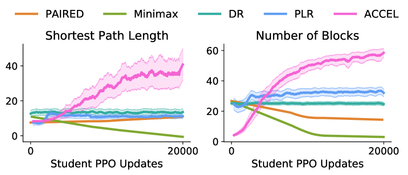
Figure 3: Emergent complexity metrics for mazes generated during training. Mean and standard error across 5 training seeds are shown.

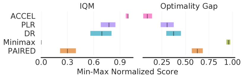
Figure 4: Aggregate zero-shot test performance in the maze domain.

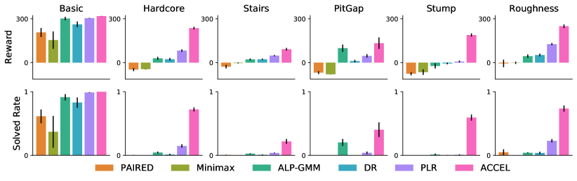
Figure 25: Test results. Agents are evaluated for 100 episodes on a series of individual challenges, plots show mean and standard error for each environment, across ten runs.

We evaluate the zero-shot transfer performance of each method on a series of held-out test environments, as done in prior works. For DR, PLR, and ACCEL, evaluation occurs after 20k student PPO updates, focusing the comparison on the effect of the curriculum. The minimax and PAIRED results are those reported in Jiang et al., 2021a at 250M training steps ($\approx$30k updates). As we see, ACCEL performs at least as well as the next best method in almost all test environments, with particularly strong performance in Labyrinth and Maze. As reported in Figure 4, ACCEL achieves drastically stronger performance than all other methods in aggregate across all test environments: Its IQM approaches a perfect solved rate compared to below 80% for the next best method, PLR, with an 80.2% probability of improvement over PLR. Detailed, per environment test results are provided in Figures 22 and 25 in Appendix B.4. Figure 5 shows example levels generated by each method. We see ACCEL produces more structured mazes than the baselines.

Next, we consider an even more challenging setting based on a larger version of PerfectMaze, a procedurally-generated maze environment, shown in Figure 7, where levels have $51\times 51$ tiles with a maximum episode length of over 5k steps—an order of magnitude larger than training levels. We evaluate agents for 100 episodes (per training seed), using the same checkpoints in Figure 4. The results in Figure 7 show ACCEL significantly outperforms all baselines with a success rate of 53% compared to the next best method, PLR, which has a success rate of 25%, while all other methods fail. Notably, successful agents approximately follow the left-hand rule for solving single-component mazes.

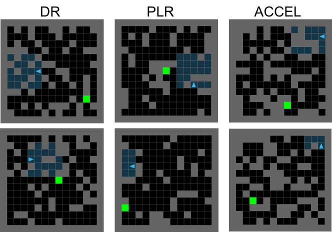
Figure 5: Example levels generated by DR, PLR, and ACCEL.

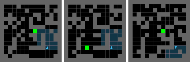
Figure 6: Despite sharing a common ancestor, each of these levels requires different behaviors to solve. Left: The agent can approach the goal by moving upwards or leftwards. Middle: The goal is on the left. Right: The left path is blocked.

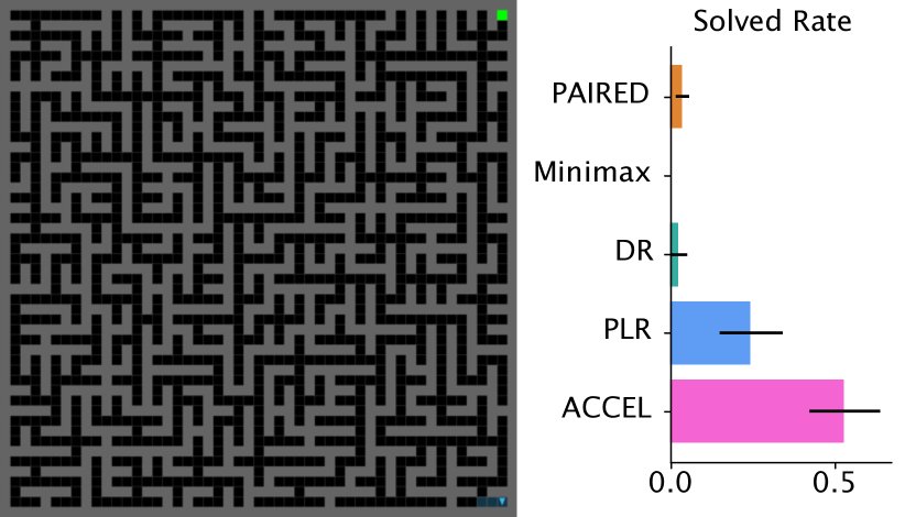
Figure 7: Zero-shot performance on a large procedurally-generated maze environment. The bars show mean and standard error over 5 training seeds, each evaluated over 100 episodes. ACCEL achieves over twice the success rate of the next best method.

We seek to understand the key drivers of ACCEL’s outperformance: Incremental changes to a level can lead to a diverse batch of new ones (Sturtevant et al.,, 2020), which may move those that are currently too hard or too easy towards the frontier of the agent’s capabilities. This diversity may prevent overfitting. For example, in Figure 6, we see three edits of the same level produced by ACCEL. Each has a similar initial observation, yet requires the agent to explore in different directions to reach the goal, thereby pressuring the agent to actively explore the environment. Further, making edits that do not change the optimal solution path can be seen as a form of data augmentation that changes the observation but not the optimal policy. Data augmentation has been shown to improve sample efficiency and robustness in RL (Laskin et al.,, 2020; Kostrikov et al.,, 2021; Raileanu et al.,, 2021).

4.2 Walking in Challenging Terrain

Finally, we evaluate ACCEL in the BipedalWalker environment from Wang et al., (2019), a continuous-control environment with dense rewards. As in Wang et al., (2019), we use a modified version of BipedalWalkerHardcore from OpenAI Gym (Brockman et al.,, 2016). We include all eight parameters in the design space, rather than only the subset used in Wang et al., (2019). This environment is detailed at length in Appendix C.1. We run all baselines from previous experiments, in addition to ALP-GMM (Portelas et al.,, 2019), which was originally tested on BipedalWalker. We train agents for 30k student updates, equivalent to between 1B to 2B total environment steps, depending on the method (see Table 10). During training we evaluate agents on both the simple BipedalWalker and more challenging BipedalWalker-Hardcore environments, in addition to four environments testing the agent’s effectiveness against specific, isolated challenges otherwise present to varying degrees in training levels: {Stump, PitGap, Stairs, Roughness}, shown in Figure 8.

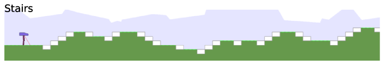
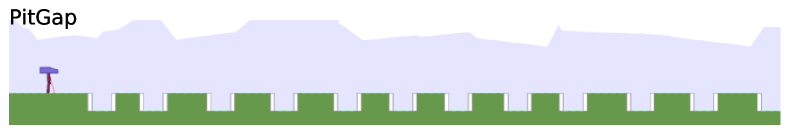
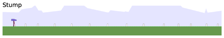
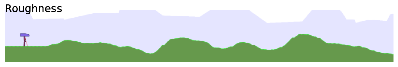
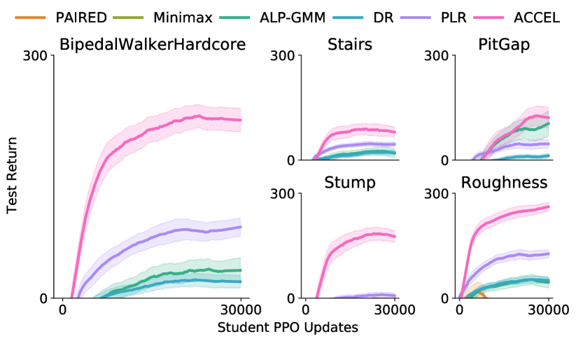
Figure 8: Top: Examples of the four individual challenges in BipedalWalker. Bottom: Performance on test environments during training (mean and standard error). Negative returns are omitted.

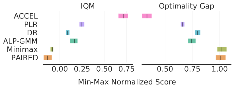
Figure 9: Aggregate performance for ten seeds across all five BipedalWalker test environments.

After 30k PPO updates, we conduct a more rigorous evaluation based on 100 test episodes in each test environment. Figure 9 reports the aggregate results, normalized according to a return range of $[0,300]$. ACCEL significantly outperforms all baselines, achieving close to 75% of optimal performance, almost three times the performance of the best baseline, PLR. All other baselines struggle, likely due to the environment design space containing a high proportion of levels not useful for learning. Faced with such challenging levels, agents may learn to resort to the locally optimal behavior of preventing itself from falling (avoiding a -100 penalty), rather than attempt forward locomotion. Finally, we see ALP-GMM performs poorly when the design space is increased from 2D (as in Portelas et al., (2019)) to 8D.

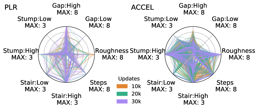
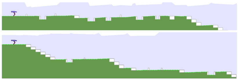
Figure 10: Top: Rose plots of complexity metrics of BipedalWalker levels discovered by PLR and ACCEL. Each line represents a solved level from the associated checkpoint. All levels are among the top-100 highest regret levels for the given checkpoint. Bottom: Two levels created and solved by ACCEL.

Next we seek to understand the properties of the evolving distribution of high-regret levels. We include all solved levels from the top-100 regret levels after 10k, 20k, and 30k student updates. For each level we show all eight parameters in Figure 10 (top), with the PLR agent as a comparison. As we see, ACCEL solves a large quantity of difficult levels of comparable difficulty with other methods such as POET, but uses a fraction of the compute. For comparison, ACCEL sees 2.07B environment steps at 30k student updates, less than 0.5% of that used in Wang et al., (2019).

4.3 POET Comparison

For a more direct comparison with POET, we train each method using 10 training seeds for 50k student PPO updates with the smaller 5D BipedalWalker environment encoding used in Wang et al., (2019). We use the thresholds provided in Wang et al., (2019), summarized in Table 1, to evaluate the difficulty of generated levels. A level meeting none of these thresholds is considered easy, while meeting one, two or three is considered challenging, very challenging or extremely challenging respectively.

Table 1: Environment encoding thresholds for 5D BipedalWalker.

Stump Height (High)	Pit Gap (High)	Ground Roughness
$\geq 2.4$	$\geq 6$	$\geq 4.5$

In Figure 11, we show the composition of the ACCEL level replay buffer during training. As we see, ACCEL produces an increasing number of extremely challenging levels as training progresses. This is a significant achievement given that POET’s evolutionary curriculum is unable to create levels in this category, without including a complex stepping-stone procedure (Wang et al.,, 2019). We thus see minimax-regret UED offers a computationally cheaper alternative to producing such levels. Moreover, POET explicitly encourages the environment parameters to reach high values through a novelty bonus, whereas the complexity discovered by ACCEL is completely emergent, arising purely through the pursuit of high-regret levels.

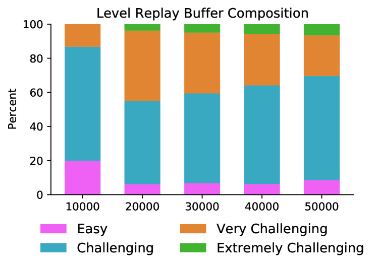
Figure 11: Percent of ACCEL level replay buffer for each difficulty. The complexity emerges purely in pursuit of high-regret levels.

While POET seeks to discover a diverse population of specialists, each capable of solving a a specific extremely challenging level, ACCEL aims to train a single generalist. To evaluate the generality of the ACCEL agent, we test all agents trained in the 5D BipedalWalker environment on the settings outlined in Figure 8, and report the results in Table 2. Note that the Stairs environment is now out-of-distribution, as the agent never sees stairs during training. As we saw in the higher-dimensional setting, the ACCEL agent is able to perform well across all settings.

Table 2: Test solved rates at 50k updates (mean and standard error) for 10 runs of each method on 100 episodes. Extremely challenging evaluation uses 1000 episodes due to the high diversity of levels. Bold values are within one standard error of the best mean.

	PLR	ALP-GMM	ACCEL
Stump	$0.04\pm 0.02$	$0.07\pm 0.02$	$\mathbf{0.44\pm 0.08}$
PitGap	$0.2\pm 0.09$	$\mathbf{0.58\pm 0.08}$	$\mathbf{0.61\pm 0.08}$
Roughness	$0.23\pm 0.04$	$0.13\pm 0.03$	$\mathbf{0.73\pm 0.03}$
Stairs	$0.02\pm 0.0$	$0.01\pm 0.0$	$\mathbf{0.12\pm 0.02}$
Hardcore	$0.21\pm 0.04$	$0.2\pm 0.04$	$\mathbf{0.65\pm 0.02}$
Extreme	$0.01\pm 0.01$	$0.02\pm 0.01$	$\mathbf{0.12\pm 0.02}$

We further test all methods on a held-out distribution of extremely challenging levels. In this case, we resample the level parameters for each episode so to ensure they meet all three criteria in Table 1. This leads to a highly diverse set of test levels. To mitigate stochasticity influencing the outcome, we evaluate each method over 1000 episodes. The results are summarized in Table 2, where we see ACCEL attains 12% average solved rate, while PLR and ALP-GMM see 1% and 2% average solved rates respectively.

Finally, we seek to evaluate our agents on specific levels produced by POET. We used the rose plots from Wang et al., (2019) to create six extremely challenging environments, each solved by one of the three POET runs. Unsurprisingly our agents find these levels challenging and see low success rates. We note that this is not a perfect comparison—POET fixes the level generator’s random seed, thereby solving a single level for each parameterization, while we repeatedly sample different levels under the same parameterization. Still, 9 out of 10 of our independent runs solved at least one of the 6 environments at least once out of 100 trials. See the Appendix (Table 7) for more detail on this experiment.

In summary, we believe ACCEL can produce levels of comparable complexity to POET, without a novelty bonus or domain-specific heuristics, at the fraction of the compute cost. Moreover, ACCEL produces a single agent robust across environment challenges, while POET results in multiple agents, each tailored to individual challenges. Therefore, we believe our method produces agents that are more robust, and thus more generally capable.

Do we need to start simple? We conduct a simple ablation study on ACCEL to test the importance of the editing mechanism and the inductive bias of starting simple. In Figure 12 we show the performance of three approaches: PLR (sample and replay DR levels), PLR+E (sample, replay, and edit DR levels) and finally PLR+E+S (i.e. ACCEL). As we see, editing levels leads to improved performance, while starting simple is more important in BipedalWalker environments.

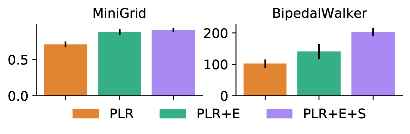
Figure 12: Aggregate returns for Editing ablations in MiniGrid and BipedalWalker. E=editing, S=start simple.

4.4 Discussion and Limitations

Our experiments demonstrate that ACCEL is capable of forming highly effective curricula in three challenging and diverse environments. In MiniGrid, we showed it is possible to produce complex mazes that facilitate zero-shot transfer to out-of-distribution, human-designed ones, including those an order of magnitude larger than the training environment. Finally, in the BipedalWalker setting we produced comparable level complexity as POET using a single agent and a small fraction of the compute cost. Our experiments provide evidence that ACCEL can be an effective curriculum method in more open-ended UED design spaces.

Importantly, the goal of our work differs from Wang et al., (2019). The primary motivation of ACCEL is to produce a single robust agent that can solve a wide range of challenges. ACCEL’s regret-based curriculum seeks to prioritize the simplest levels that the agent cannot currently solve. In contrast, POET co-evolves agent-environment pairs in order to find specialized policies for solving a single highly specialized task. POET’s specialized agents may likely learn to solve challenging environments outside the capabilities of ACCEL’s generalist agents, but at the cost of potentially overfitting to their paired levels. Thus, unlike ACCEL, the policies produced by POET should not be expected to be robust across the full distribution of levels. The relative merits of POET and ACCEL thus highlight an important trade-off between specialization and generalization, both of which may ultimately be important for solving more complex, larger scale problems.

While ACCEL’s simplicity is appealing, larger design spaces may require additional mechanisms, like actively promoting diversity in level design. Moreover, ACCEL uses an inductive bias by starting with the simplest base case (e.g. an empty room), which may not always be possible in practice. In some settings, simple levels for agents may be more complex in design, e.g. in a Hide-and-Seek game.

5 Related Work

Table 3: The components of related approaches. Like POET, ACCEL evolves levels, but only trains a single agent while using a minimax-regret objective to ensure levels are solvable. PAIRED uses minimax regret to train the generator, and does not replay levels. Finally, PLR curates levels using minimax regret, but relies solely on domain randomization for generation.

Algorithm	Generation Strategy	Generator Obj	Curation Obj	Output
POET (Wang et al.,, 2019)	Evolution	Minimax	MCC	Specialists
PAIRED (Dennis et al.,, 2020)	Reinforcement Learning	Minimax Regret	None	Generalist
PLR (Jiang et al., 2021b, ; Jiang et al., 2021a, )	Random	None	Minimax Regret	Generalist
ACCEL	Random + Evolution	None	Minimax Regret	Generalist

In this section we provide a brief overview of related work. We provide a more detailed discussion in Appendix A.

The goal of this work is to produce agents that are capable of systematic generalization across a wide range of environments (Whiteson et al.,, 2009), which has recently been a focus for the deep RL community (Packer et al.,, 2019; Igl et al.,, 2019; Cobbe et al.,, 2020; Agarwal et al., 2021a, ; Zhang et al., 2018b, ; Ghosh et al.,, 2021). A common approach for producing robust agents is Domain Randomization (DR, Jakobi, (1997); Sadeghi and Levine, (2017)), widely used in robotics (Tobin et al.,, 2017; James et al.,, 2017; Andrychowicz et al.,, 2020; OpenAI et al.,, 2019).

The evolutionary component of ACCEL is inspired by the open-ended creative potential of POET (Wang et al.,, 2019, 2020; Brant and Stanley,, 2017; Dharna et al.,, 2020), which seeks to train a population of highly capable specialists. By contrast, ACCEL trains a single generally capable agent with a regret-based curriculum as in PAIRED (Dennis et al.,, 2020) and Robust PLR (Jiang et al., 2021a, ) (see Table 3). These methods for Unsupervised Environment Design (UED, Dennis et al.,, 2020), naturally relate to the field of Automatic Curriculum Learning (ACL, Portelas et al.,, 2020; Florensa et al.,, 2017; Baranes and Oudeyer,, 2009), with the key difference being that in UED all elements of the POMDP are underspecified.

Our work also closely relates to previous environment design literature in the symbolic AI commmunity (Zhang and Parkes,, 2008; Zhang et al.,, 2009; Keren et al.,, 2017, 2019), though our focus falls primarily on generating curricula. Finally, we take inspiration from the field of procedural content generation (PCG; Risi and Togelius,, 2020; Justesen et al.,, 2018), which seeks to produce a distribution of levels for a given environment, often using machine learning (Summerville et al.,, 2018; Bhaumik et al.,, 2020; Liu et al.,, 2021). We are particularly inspired by PCGRL (Khalifa et al.,, 2020; Earle et al., 2021a, ) which frames level design as an RL problem, making incremental changes to a level to maximize some objective subject to game-specific constraints.

6 Conclusion and Future Work

We proposed ACCEL, a new method for unsupervised environment design (UED), that evolves a curriculum by editing previously curated levels. Editing induces an evolutionary process that leads to a wide variety of environments at the frontier of the agent’s capabilities, producing curricula that start simple and quickly compound in complexity. Thus, ACCEL provides a principled regret-based curriculum that exploits an evolutionary process to produce a broad spectrum of environment complexity matched to the agent’s current capabilities. Importantly, ACCEL avoids the need for domain-specific heuristics. In our experiments, we showed that ACCEL is capable of training robust agents in a series of challenging design spaces, where ACCEL agents outperform the best-performing baselines.

We are excited by the many possibilities for extending how ACCEL edits and maintains its population of high-regret levels. The editing mechanism could encompass a wide variety of approaches, such as Neural Cellular Automata (Earle et al., 2021b, ), controllable editors (Earle et al., 2021a, ), or perturbing the latent space of a generative model (Fontaine et al.,, 2021). Another possibility is to actively seek levels which are likely to produce useful levels in the future (Gajewski et al.,, 2019). Moreover, ACCEL’s evolutionary search may be expedited by introducing so-called extinction events (Raup,, 1986; Lehman and Miikkulainen,, 2015), believed to play a crucial role in natural evolution. We did not explore methods to encourage level diversity, but such diversity is likely important for larger design spaces, such as 3D control tasks that transfer more directly to the real world. It remains an open question whether producing sufficient diversity would require a population, for example using the domain-agnostic, population-based novelty objective in Enhanced POET (Wang et al.,, 2020). We believe such ideas at the intersection of evolution and adaptive curricula can take us closer to producing a truly open-ended learning process between the agent and the environment (Stanley et al.,, 2017). Finally, we note that while ACCEL may be an effective approach for automatically generating an effective curriculum, it may still be necessary to likewise adapt the agent configuration (Parker-Holder et al.,, 2022) to most effectively train agents in open-ended environments.

Appendix A Extended Related Work

Our paper focuses on testing agents on distributions of environments, long known to be crucial for evaluating the generality of RL agents (Whiteson et al.,, 2009). The inability of deep RL agents to reliably generalize across distributions of environment configurations has drawn considerable attention (Packer et al.,, 2019; Igl et al.,, 2019; Cobbe et al.,, 2020; Agarwal et al., 2021a, ; Zhang et al., 2018b, ; Ghosh et al.,, 2021), with policies often failing to adapt to changes in the observation (Song et al.,, 2020), dynamics (Ball et al.,, 2021), or reward (Zhang et al., 2018a, ). In this work, we seek to provide agents with a set of training levels to produce a policy that is robust to such variations.

In particular, we focus on the Unsupervised Environment Design (UED, Dennis et al.,, 2020) paradigm, which aims to design environment directly, such that they induce experiences that result in learning more robust policies. Domain Randomization (DR, Jakobi,, 1997; Sadeghi and Levine,, 2017), which simply randomizes the environment configuration, can be viewed as the most basic form of UED. DR has been particularly successful in areas such as robotics (Tobin et al.,, 2017; James et al.,, 2017; Andrychowicz et al.,, 2020; OpenAI et al.,, 2019), with extensions that actively update the DR distribution (Mehta et al.,, 2020; Raparthy et al.,, 2020). This paper directly extends Prioritized Level Replay (PLR, Jiang et al., 2021b, ; Jiang et al., 2021a, )), a method for curating DR levels such that only those with high learning potential are revisited by the student agent for training. PLR is related to TSCL (Matiisen et al.,, 2020), self-paced learning (Klink et al.,, 2019; Eimer et al.,, 2021), and ALP-GMM (Portelas et al.,, 2019), which all seek to maintain and update distributions over informative environment parameterizations based on the recent performance of the agent. Recently, a method similar to PLR was shown to be capable of producing generally-capable agents in a simulated game world with a smooth space of levels (Team et al.,, 2021).

Dennis et al., (2020) first formalized UED and introduced the PAIRED algorithm, a minimax-regret (Savage,, 1951) UED algorithm whereby an environment adversary learns to present levels that maximize regret, approximated as the difference in performance between the main student agent and a second student agent. PAIRED produces agents with improved zero-shot transfer to unseen environments and has been extended to train agents that can robustly navigate websites (Gur et al.,, 2021). Adversarial objectives have also been considered in robotics (Pinto et al.,, 2017) and in directly searching for situations in which the agent sees the weakest performance (Everett et al.,, 2019). POET (Wang et al.,, 2019, 2020) considers co-evolving a population of minimax environments and agents that solve them. ACCEL harnesses the evolutionary potential of POET while training only a single agent, which takes significantly less resources, while also avoiding the agent selection problem.

UED is related to Automatic Curriculum Learning (ACL, Portelas et al.,, 2020; Florensa et al.,, 2017; Baranes and Oudeyer,, 2009), which seeks to provide an adaptive curriculum of increasingly challenging tasks or goals (Andrychowicz et al.,, 2017). This setting differs from a general UPOMDP, which aims to actively generate the entire environment given a domain specification and where the free parameters, e.g. the task or goal specifier, are typically not fully observed. In Asymmetric Self-Play (Sukhbaatar et al.,, 2018; OpenAI et al.,, 2021), the agent’s goal is based on reversing the trajectory of another; this process leads to effective curricula for robotic manipulation tasks. AMIGo (Campero et al.,, 2021) and APT-Gen (Fang et al.,, 2021) produce adaptive curricula for hard-exploration, goal-conditioned problems. Many ACL methods focus on learning to reach goals or states with high uncertainty (Racaniere et al.,, 2020; Pong et al.,, 2020; Zhang et al.,, 2020), including latent states inside a generative model (Florensa et al.,, 2018; Mendonca et al.,, 2021).

Automatic environment design has also been considered in the symbolic AI community as a means to shape an agent’s decisions (Zhang and Parkes,, 2008; Zhang et al.,, 2009) Automated environment design (Keren et al.,, 2017, 2019) seeks to redesign specific levels to improve the agent’s performance within them. In contrast, UED adapts curricula that improves performance across levels.

Our work also relates to the field of procedural content generation (PCG; Risi and Togelius,, 2020; Justesen et al.,, 2018), which has studied the algorithmic generation of game levels for over a decade (Togelius and Schmidhuber,, 2008). Popular PCG environments used in RL include the Procgen Benchmark (Cobbe et al.,, 2020), MiniGrid (Chevalier-Boisvert et al.,, 2018), Obstacle Tower (Juliani et al.,, 2019), GVGAI (Perez-Liebana et al.,, 2019), and the NetHack Learning Environment (Küttler et al.,, 2020). This work uses the MiniHack environment (Samvelyan et al.,, 2021), which provides a flexible framework for creating diverse environments. Many recent PCG methods use machine learning (Summerville et al.,, 2018; Bhaumik et al.,, 2020; Liu et al.,, 2021). PCGRL (Khalifa et al.,, 2020; Earle et al., 2021a, ) frames level design as an RL problem, whereby the design policy incrementally changes the level to maximize some objective subject to game-specific constraints. Unlike ACCEL, it makes use of hand-designed dense rewards and focuses on the design of levels for human players, rather than as an avenue to training highly-robust agents.

Appendix B Additional Experimental Results

B.1 Learning with Lava

Here we explore a simple proof of concept: a grid environment, where the agent must navigate to a goal in the presence of lava blocks. The grid is only $7\times 7$, but remains challenging as the episode terminates with zero reward if the agent touches the lava. This dynamic makes exploration more difficult by penalizing random actions. While toy, such challenges may be relevant in real-world, safety-critical settings, where agents may wish to avoid events causing early termination during training. For DR and PLR, the random generator samples the number of lava tiles to place from the range $[0,20]$. For ACCEL, we use a generator that produces empty rooms and then proceeds to edit the levels by adding or removing lava tiles. The environment is built with MiniHack (Samvelyan et al.,, 2021) and is fully observable with a high-dimensional input. The full environment details are provided in C.1.

Figure 13 shows the results of running each method over 5 random seeds. Despite starting with empty rooms, ACCEL quickly produces levels with more lava than the other methods, while also attaining higher training returns, reaching near-perfect performance on its training distribution. This behavior is entirely driven by the pursuit of high-regret levels, which constantly seeks the frontier of the agent’s capabilities. PLR is able to produce a similar training profile to ACCEL, but achieves lower values for each complexity metric.

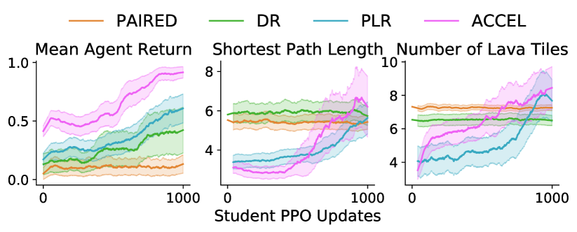
Figure 13: Training return and emergent complexity in Lava Grid. The plots report the mean and standard error over 5 seeds.

We evaluate each agent on a series of test levels after 1000 PPO updates (approximately 20M timesteps), and report the aggregate results in Figure 14, where we see that ACCEL is the best performing method. Extended results are shown in Table 4. The first three test environments (Empty, 10 Tiles and 20 Tiles) evaluate the performance of the agent within its training distribution, while we also include a held-out human designed environment, LavaCrossing S9N1, ported from MiniGrid (Chevalier-Boisvert et al.,, 2018). As we see, ACCEL performs best on all of the in-distribution environments (whose levels can be directly sampled in the training distribution), while also being only one of two approaches to get meaningfully above zero in the human designed task.

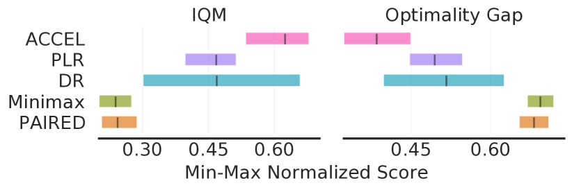
Figure 14: Lava Grid aggregate test performance.

Table 4: Test performance in in-distribution and out-of-distribution environments. Each entry is the mean (and standard error) of 5 independent training runs, where each run is evaluated for 100 trials on each environment. $\dagger$ indicates the generator’s per-tile lava distribution is binomial and the generator can place lava in 20 blocks. $\ddagger$ indicates the generator first samples the number of lava tiles to place (in $[0,20]$), then places that many at random locations. Bold values are within one standard error of the best mean.

Test Environment	PAIRED	Minimax	DR$\dagger$	PLR$\dagger$	DR$\ddagger$	PLR$\ddagger$	ACCEL
Empty	$0.77\pm 0.03$	$0.76\pm 0.02$	$0.81\pm 0.03$	$0.97\pm 0.03$	$0.89\pm 0.05$	$0.96\pm 0.04$	$\mathbf{1.0\pm 0.0}$
10 Tiles	$0.12\pm 0.03$	$0.05\pm 0.01$	$0.12\pm 0.02$	$0.35\pm 0.18$	$0.33\pm 0.15$	$0.3\pm 0.05$	$\mathbf{0.49\pm 0.07}$
20 Tiles	$0.06\pm 0.01$	$0.11\pm 0.04$	$0.06\pm 0.01$	$0.15\pm 0.09$	$0.23\pm 0.12$	$0.25\pm 0.06$	$\mathbf{0.35\pm 0.08}$
LavaCrossing S9N1	$0.0\pm 0.0$	$0.0\pm 0.0$	$0.0\pm 0.0$	$0.01\pm 0.01$	$\mathbf{0.05\pm 0.05}$	$0.01\pm 0.0$	$\mathbf{0.05\pm 0.04}$

B.2 Level Evolution

In Fig 16 and 16, we show levels produced by ACCEL for the MiniHack lava environment and MiniGrid mazes respectively. Each step along the evolutionary process produces a level that has high learning potential at that point in training.

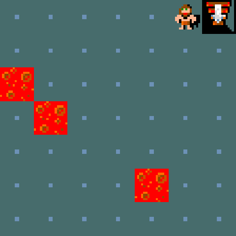
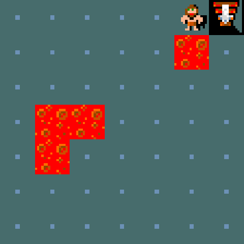
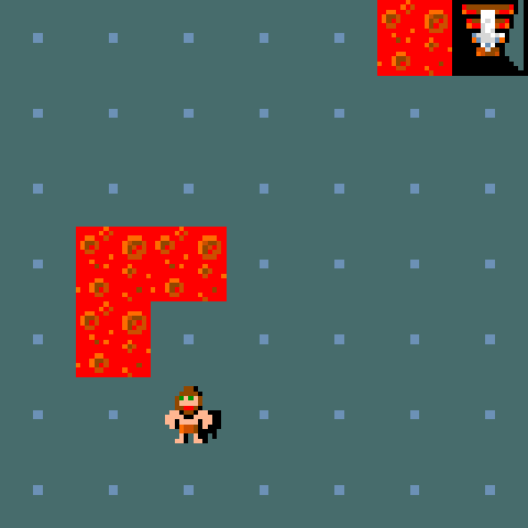
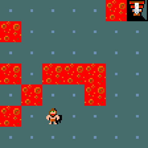
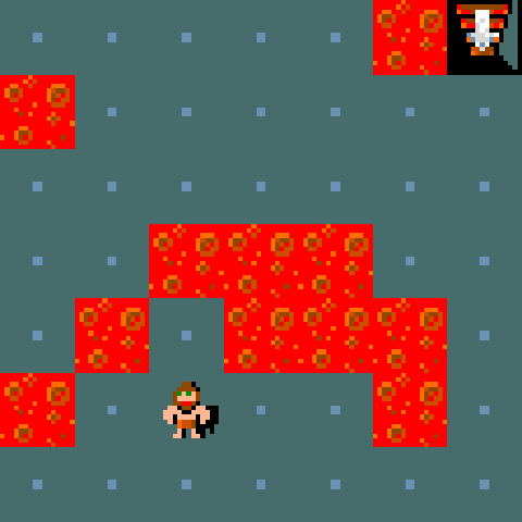
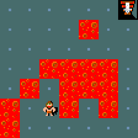
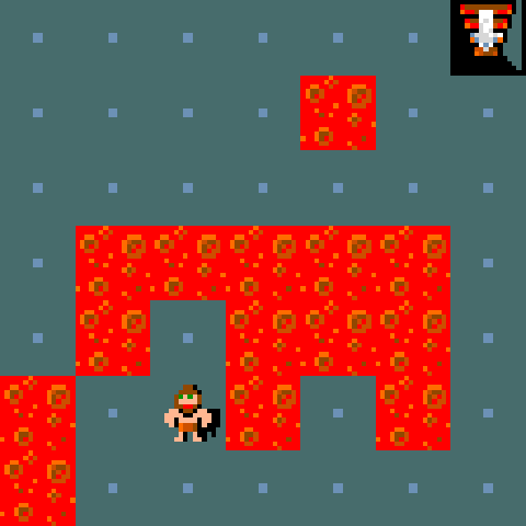
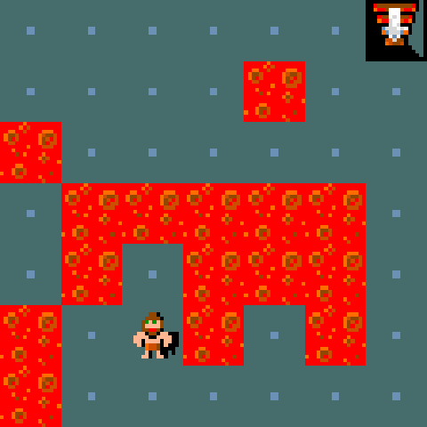
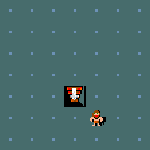
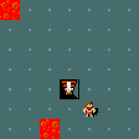
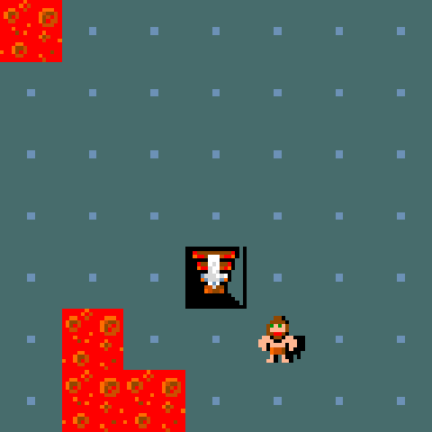
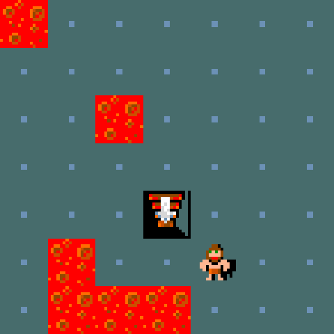
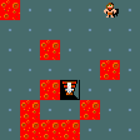
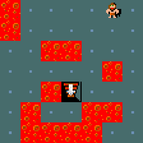
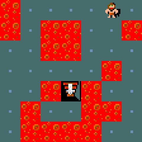
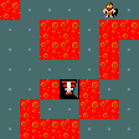
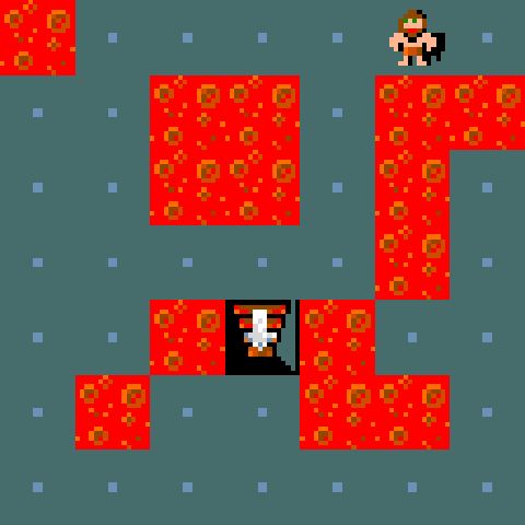
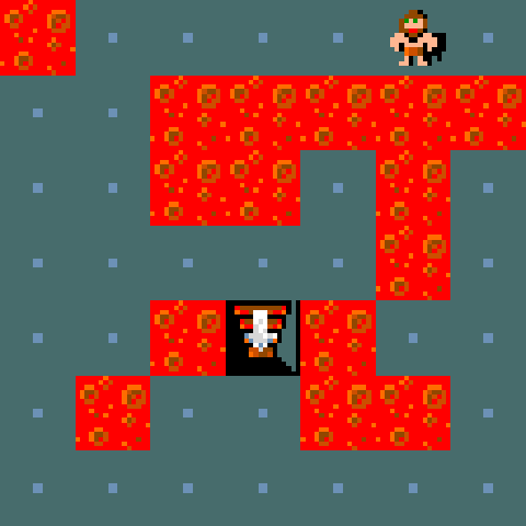
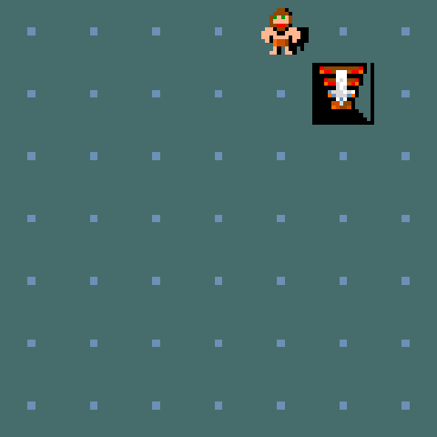
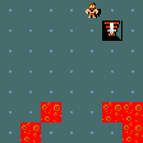
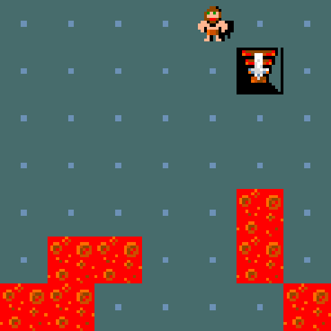
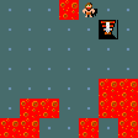
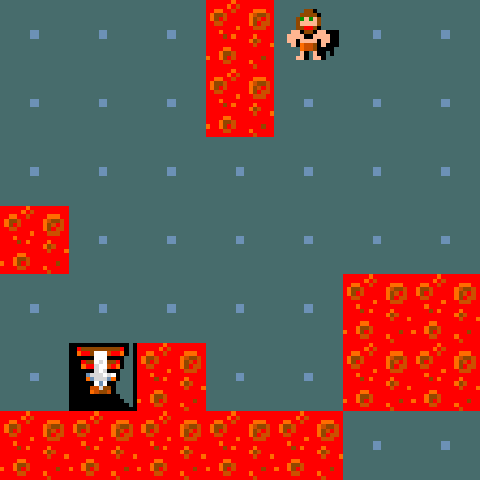
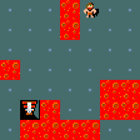
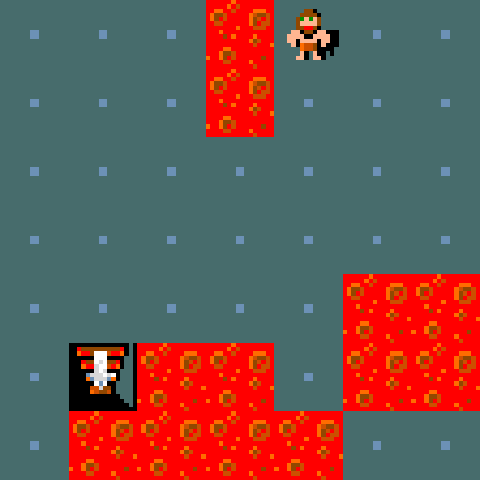
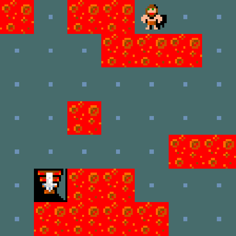
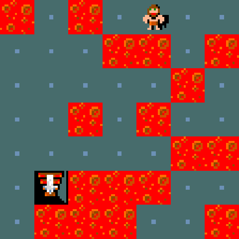
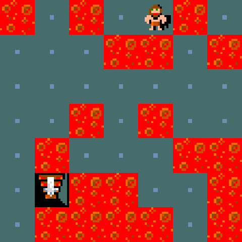
Figure 15: Levels generated by ACCEL. Each level along the evolutionary path is at the frontier for the student agent at that stage of training. As we can see, the edits compound to produce a series of challenges: In the first level the lava gradually surrounds the agent, such that they can initially explore in multiple directions, but near the end the task can only be solved by going down and to the right. In the middle row, we see a level where the agent has a direct path to the goal, but a corridor is evolved over time to become increasingly narrow, before being filled in so the agent has to go around it. Finally in the bottom row the level begins with simple augmentations before moving the agent behind a barrier, which results in a challenging task where the agent has to move in a diagonal direction to escape the lava.

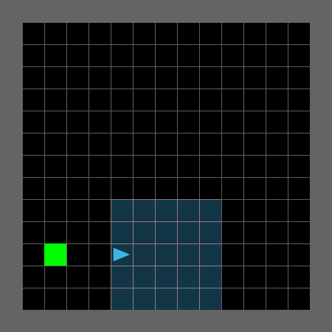
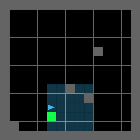
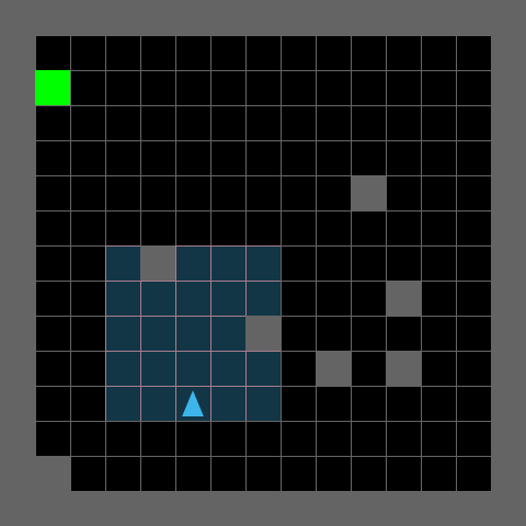
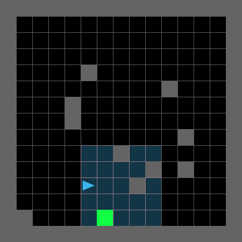
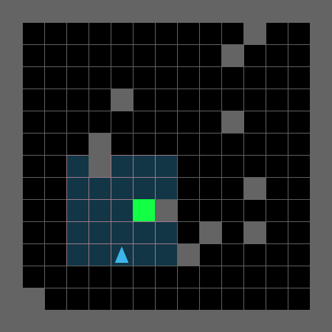
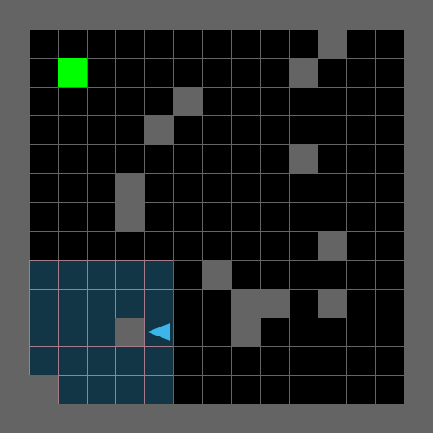
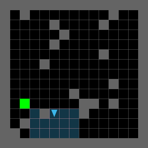
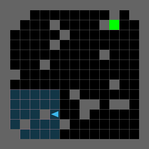
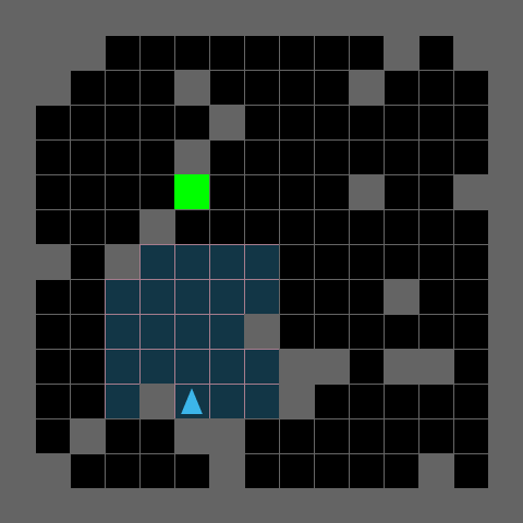
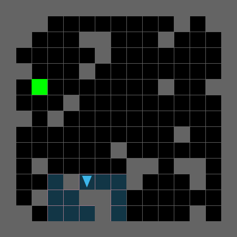
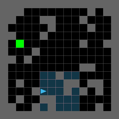
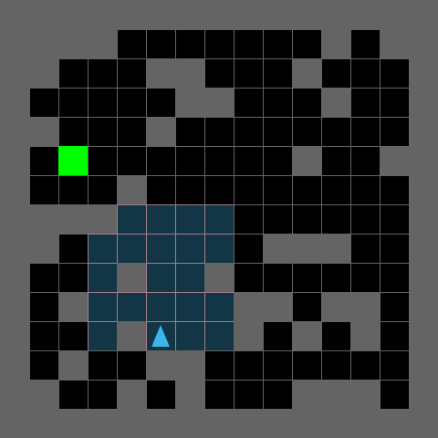
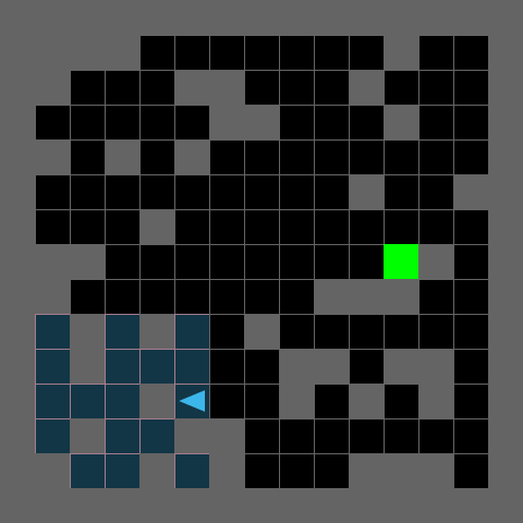
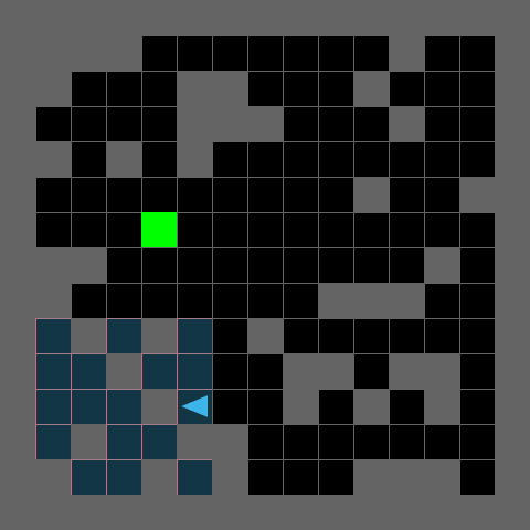
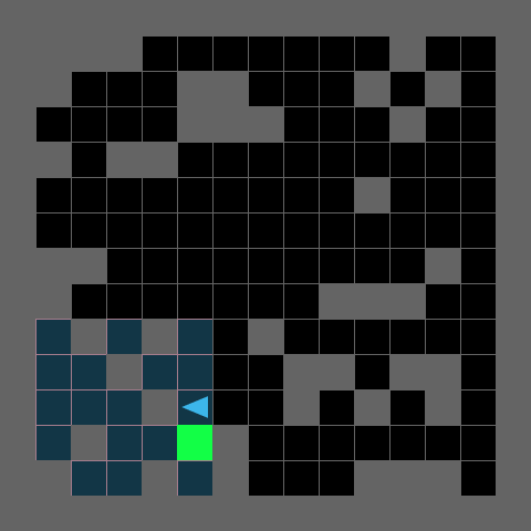
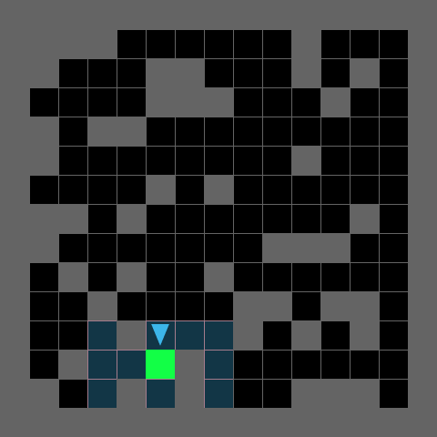
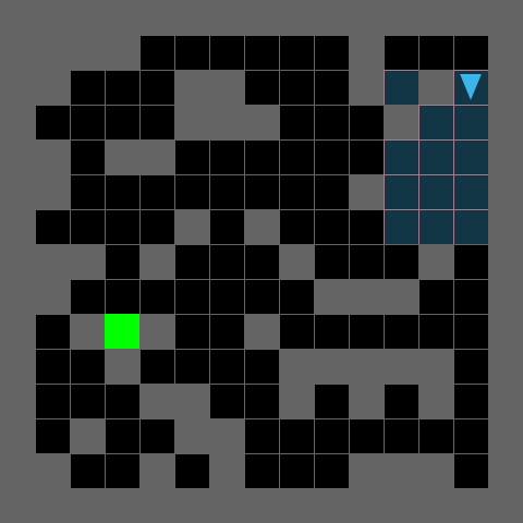
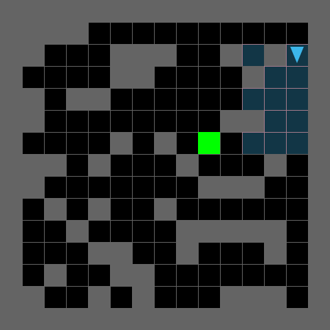
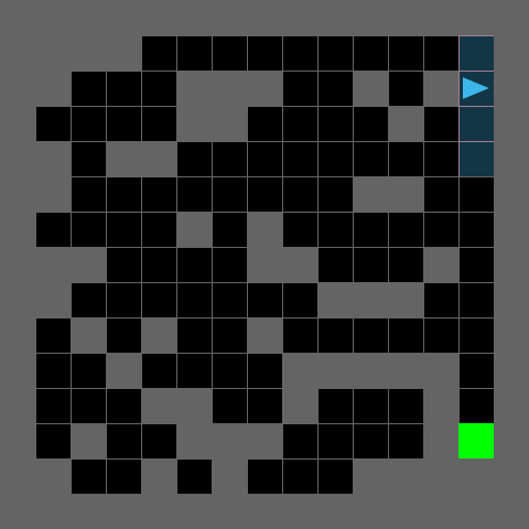
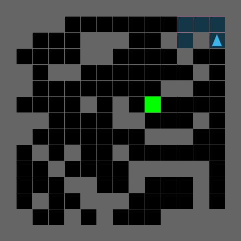
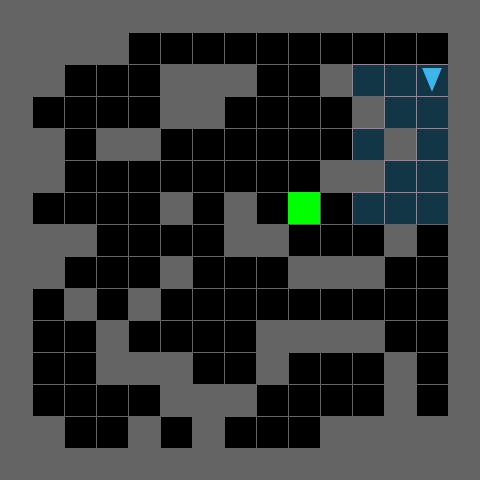
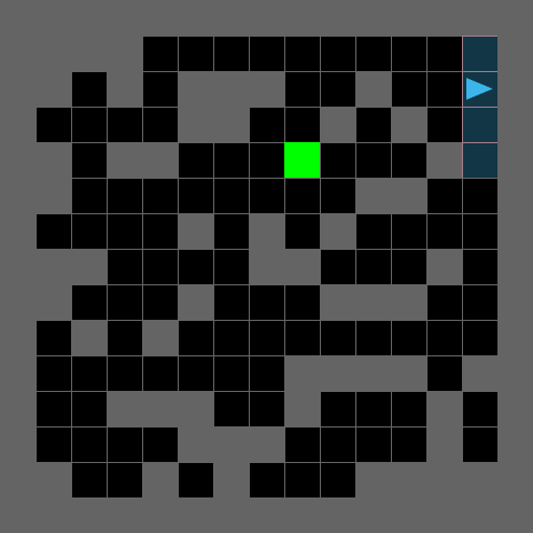
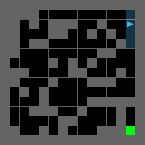
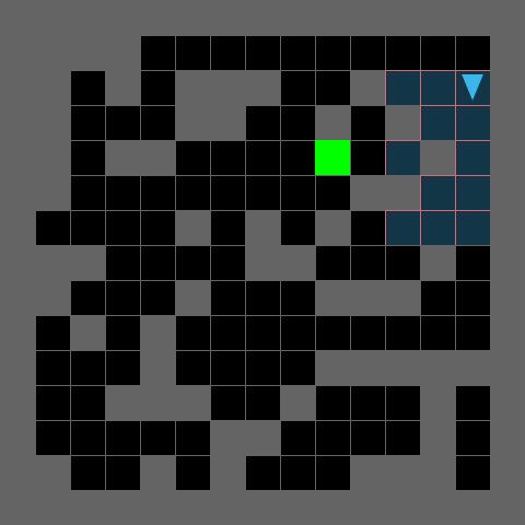
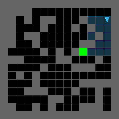
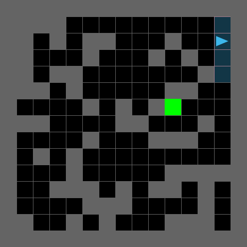
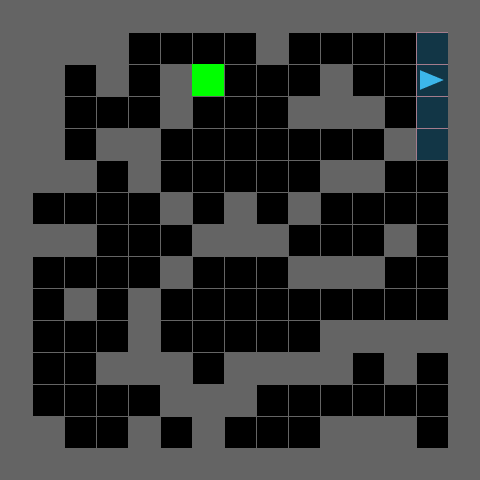
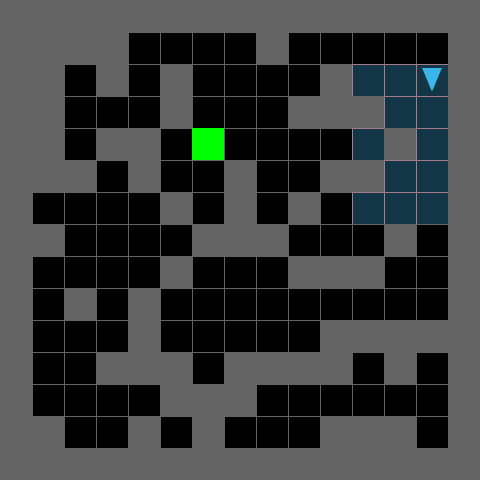
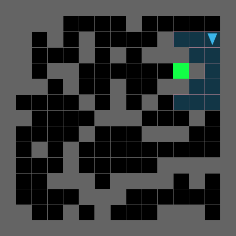
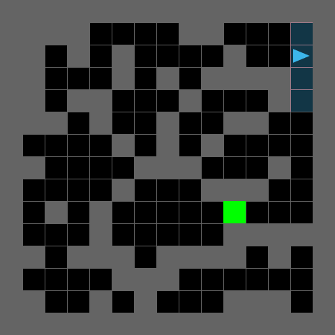
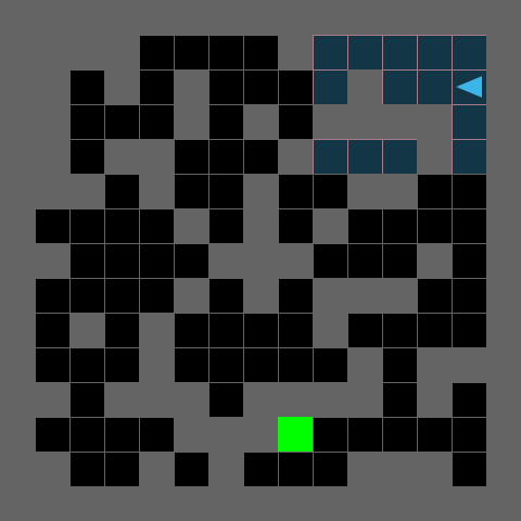
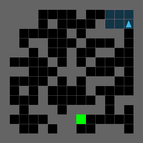
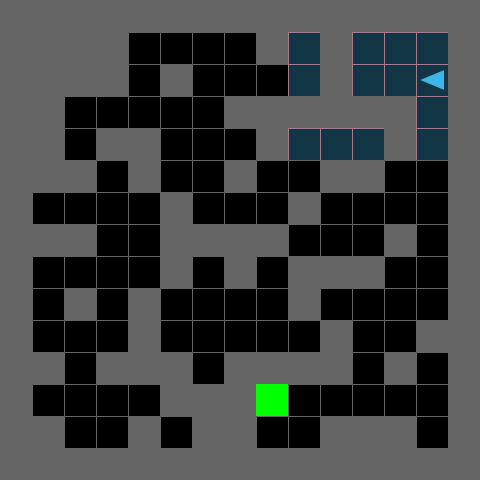
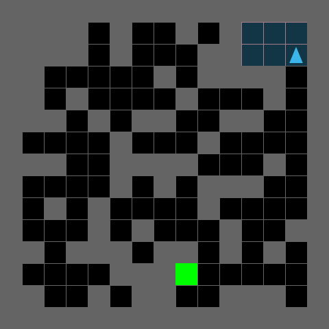
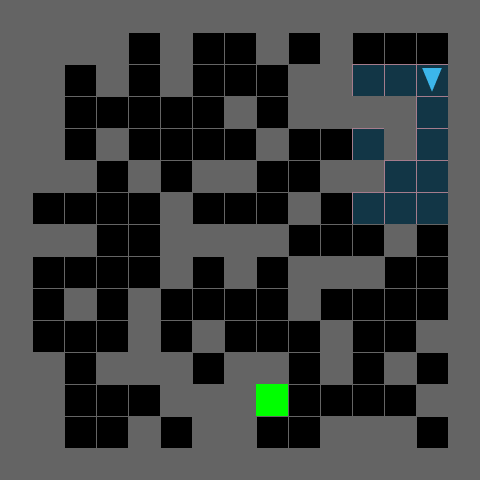
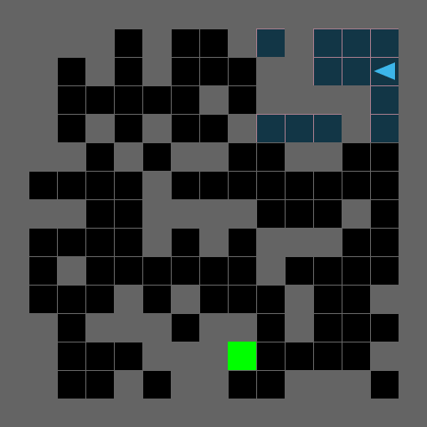
Figure 16: The evolution of a single level the MiniGrid environment, starting from top-left, ending bottom-right. Throughout the process the agent experiences a diverse set of challenges.

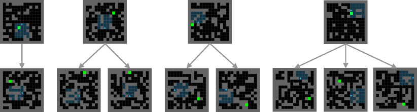
Figure 17: Maze evolution. Top row shows starting levels, originally included in the PLR buffer due to having high positive value loss. After many edits (up to 40), ACCEL produces the bottom row, which were all selected from the top-50 levels in terms of PLR scores after 10k gradient steps. As we see, the same level can produce distinct future levels, in some cases multiple high-regret levels.

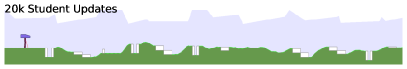
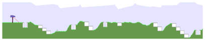
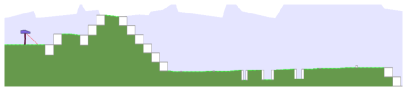
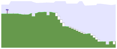
Figure 18: Levels created and solved by ACCEL in the BipedalWalker environment. At the beginning (top row) levels are initialized with low values for environment parameters, encoding the range of obstacle sizes. After several edits, we reach challenging scenarios like steep staircases or high stumps. By the end of training, we see a diverse combination of multiple challenges.

B.3 The Expanding Frontier

Here we analyze the performance of agents on levels produced by ACCEL. We inspect four agent checkpoints, from 5k, 10k, 15k and 20k student updates. In Figure 19 we show four generations of a level. We see that the later generations become harder for the 5k checkpoint, while the 20k checkpoint sees the highest return from the more complex level in Gen 63.

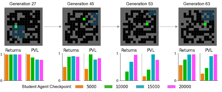
Figure 19: The Evolving Frontier. The top row shows four levels from the same lineage, at generations 27, 45, 53 and 63. Underneath each is a bar plot showing the return and positive value loss (PVL) for four different ACCEL policies, checkpointed at 5k, 10k, 15k and 20k PPO updates. At generation 27, all four checkpoints can solve the level, but the 5k checkpoint has the highest learning potential (PVL). On the right we see that by generation 63, only the 15k and 20k checkpoints are able to achieve a high return on the level.

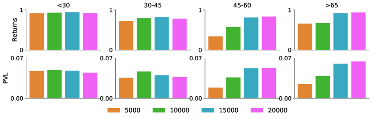
Figure 20: Aggregate metrics for each band of generations. For example, “30-45” refers to all the levels between generation 30-45. The later generation levels are harder for the early agents to solve, while the early agents have higher return and PVL for the earlier levels.

In Figure 20 we show all generations for the level included in Figure 19, grouped by generation. We then show the mean return and PVL for all four agent checkpoints. We find the 20k checkpoint sees the highest learning potential in levels from later generations, while the 5k checkpoint sees the lowest return on these levels. Next in Figure 21 we show data for all generations of 20 levels which were present in the 20k checkpoint replay buffer and their ancestors in the 5k checkpoint buffer. For each checkpoint, we visualize the solved rate for each of these levels based the color of the point for each level, plotted along axes corresponding to shortest path length and number of blocks. The 5k checkpoint can only reliably solve the shorter-path levels with low block count. In contrast, the 20k checkpoint performs well across all sampled levels.

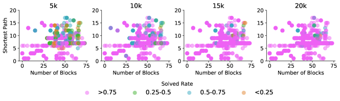
Figure 21: How do complexity metrics relate to difficulty? The plot shows the block count and shortest path length. From left to right we evaluate the agents at four checkpoints: 5k, 10k, 15k, 20k PPO updates. The color represents the solved rate. As we see, the 5k agent is unable to solve the levels with higher block count and longer paths to the goal, while the 20k agent is able to solve almost all levels.

B.4 Full Experimental Results

Partially-Observable Navigation Next we show the extended results for the MiniGrid experiments. We use a series of challenging zero-shot environments (see Figure 22), introduced in the UED literature (Dennis et al.,, 2020; Jiang et al., 2021a, ). We include the full results in Table 5 and bar plots of the same data in Figure 25.

We also include an additional version of ACCEL using the same generator as the DR and PLR baselines, thus editing more complex base levels. This removes the prior that it is beneficial to begin with simple empty rooms. As we see, both versions of ACCEL significantly outperform the baselines. Particularly in the more complex environments like Labyrinth, we see large gains compared to baselines. Also note that PLR outperforms all other baselines, and ACCEL outperforms PLR. We show report these results in the Table 22, as well as show more robust comparison metrics provided by rliable (Agarwal et al., 2021b, ) in Figure 24.

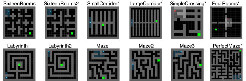
Figure 22: MiniGrid Zero-Shot Environments. Those with an asterisk are procedurally generated: For SmallCorridor and LargeCorridor, the position of the goal can be in any of the corridors. SimpleCrossing and FourRooms are from Chevalier-Boisvert et al., (2018), and PerfectMaze, from Jiang et al., 2021a .

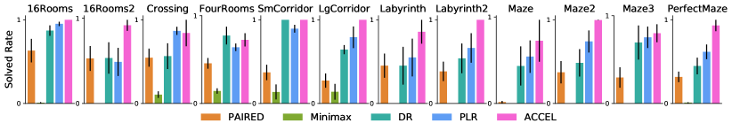
Figure 23: Zero-shot transfer results in out-of-distribution mazes. Agents are evaluated for 100 episodes on human-designed mazes. Plots show mean and standard error for each environment, across five runs.

Table 5: Zero-Shot transfer to human-designed environments. Each entry corresponds to the mean and standard error of 5 training runs, where each run is evaluated for 100 trials on each environment. $\dagger$ indicates the generator first samples the number of blocks to place in $[0,60]$, then places that many at random locations. $\ddagger$ indicates the generator produces only empty rooms. Bold values are within one standard error of the best mean. $\star$ indicates a statistically significant improvement against PLR ($p<0.05$ via Welch’s t-test). All methods are evaluated after 20k student updates, aside from PAIRED and Minimax, which are evaluated at $\approx$30k updates.

Environment	PAIRED	Minimax	DR$\dagger$	PLR$\dagger$	ACCEL$\dagger$	ACCEL$\ddagger$
16Rooms	$0.63\pm 0.14$	$0.01\pm 0.01$	$0.87\pm 0.06$	$0.95\pm 0.03$	$\mathbf{1.0\pm 0.0}$	$\mathbf{1.0\pm 0.0}$
16Rooms2	$0.53\pm 0.15$	$0.0\pm 0.0$	$0.53\pm 0.18$	$0.49\pm 0.17$	$0.62\pm 0.22$	$\mathbf{0.92\pm 0.06}$
SimpleCrossing	$0.55\pm 0.11$	$0.11\pm 0.04$	$0.57\pm 0.15$	$\mathbf{0.87\pm 0.05}$	$\mathbf{0.92\pm 0.08}$	$\mathbf{0.84\pm 0.16}$
FourRooms	$0.46\pm 0.06$	$0.14\pm 0.03$	$0.77\pm 0.1$	$0.64\pm 0.04$	$\mathbf{0.9\pm 0.08}$	$0.72\pm 0.07$
SmallCorridor	$0.37\pm 0.09$	$0.14\pm 0.09$	$\mathbf{1.0\pm 0.0}$	$0.89\pm 0.05$	$0.88\pm 0.11$	$\mathbf{1.0\pm 0.0}$
LargeCorridor	$0.27\pm 0.08$	$0.14\pm 0.09$	$0.64\pm 0.05$	$0.79\pm 0.13$	$0.94\pm 0.05$	$\mathbf{1.0\pm 0.0}$
Labyrinth	$0.45\pm 0.14$	$0.0\pm 0.0$	$0.45\pm 0.23$	$0.55\pm 0.23$	$\mathbf{0.97\pm 0.03}$	$0.86\pm 0.14$
Labyrinth2	$0.38\pm 0.12$	$0.0\pm 0.0$	$0.54\pm 0.18$	$0.66\pm 0.18$	$\mathbf{1.0\pm 0.01}$	$\mathbf{1.0\pm 0.0}$
Maze	$0.02\pm 0.01$	$0.0\pm 0.0$	$0.43\pm 0.23$	$\mathbf{0.54\pm 0.19}$	$\mathbf{0.52\pm 0.26}$	$\mathbf{0.72\pm 0.24}$
Maze2	$0.37\pm 0.13$	$0.0\pm 0.0$	$0.49\pm 0.16$	$0.74\pm 0.13$	$0.93\pm 0.04$	$\mathbf{1.0\pm 0.0}$
Maze3	$0.3\pm 0.12$	$0.0\pm 0.0$	$0.69\pm 0.19$	$0.75\pm 0.12$	$\mathbf{0.94\pm 0.06}$	$0.8\pm 0.1$
PerfectMaze (M)	$0.32\pm 0.06$	$0.01\pm 0.0$	$0.45\pm 0.1$	$0.62\pm 0.09$	$\mathbf{0.88\pm 0.12}$	$\mathbf{0.93\pm 0.07}$
Mean	$0.39\pm 0.03$	$0.05\pm 0.01$	$0.62\pm 0.05$	$0.71\pm 0.04$	$\mathbf{0.88\pm 0.04}^{\star}$	$\mathbf{0.9\pm 0.03}^{\star}$

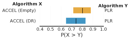
Figure 24: Probability of improvement of ACCEL over PLR across all evaluation environments in Figure 22, using the open-source notebook from Agarwal et al., 2021b . The probability of improvement represents the probability that Algorithm X outperforms Algorithm Y on a new task from the same distribution.

BipedalWalker For the BipedalWalker environment, we test agents on each of the individual challenges encoded in the environment parameterization. Specifically, we evaluate agents in the following four environments:

• Stairs: The stair height parameters are set to [2,2] with the number of steps set to 5.

• PitGap: The pit gap parameter is set to [5,5].

• Stump: The stump parameter is set to [2,2].

• Roughness: The ground roughness parameter is set to 5.

Each of these environments is visualized in Figure 8 in the main paper. We also test agents on the simple BipedalWalker-v3 environment and the more challenging BipedalWalkerHardcore-v3 environment. For BipedalWalkerHardcore-v3, we note that none of our agents fully solve the environment, which is considered to be a mean reward $ge300$ over 100 independent evaluations. To test whether it is possible with our base RL algorithm and agent model, we trained an identical PPO agent directly on the environment for 1B steps. The reward achieved was 239—indistinguishable from that achieved by ACCEL, which additionally robustifies the agent against a much wider range of environments, including the individual challenges described above.

Table 6: Test performance on a variety of challenging evaluation environments. Each entry corresponds to the mean and standard error of 10 independent runs, where each run is evaluated for 100 trials on each environment. $\dagger$ indicates the generator creates each level with obstacle parameters uniformly sampled between the corresponding minimum value of the “Easy Init” range and max value defined in Table 9. $\ddagger$ indicates the generator instead uniformly samples obstacle parameters within the “Easy Init” ranges. Bold indicates being within one standard error of the best mean. All methods are evaluated at 30k updates.

Environment	PAIRED	Minimax	ALP-GMM	DR$\dagger$	PLR$\dagger$	ACCEL$\dagger$	ACCEL$\ddagger$
Basic	$206.5\pm 30.3$	$154.3\pm 59.2$	$301.5\pm 11.6$	$261.9\pm 19.3$	$304.1\pm 1.8$	$316.9\pm 2.1$	$\mathbf{318.1\pm 1.0}$
Hardcore	$-47.2\pm 10.6$	$-44.3\pm 1.6$	$29.7\pm 9.9$	$23.8\pm 8.3$	$82.6\pm 8.5$	$163.3\pm 30.9$	$\mathbf{236.0\pm 8.9}$
Stairs	$-27.4\pm 12.1$	$-2.6\pm 2.6$	$22.1\pm 6.3$	$23.3\pm 4.4$	$48.0\pm 4.3$	$59.4\pm 10.5$	$\mathbf{91.7\pm 8.9}$
PitGap	$-68.2\pm 9.7$	$-79.3\pm 0.5$	$\mathbf{98.8\pm 24.9}$	$11.0\pm 7.6$	$46.2\pm 11.3$	$49.6\pm 12.6$	$\mathbf{133.3\pm 39.1}$
Stump	$-76.0\pm 10.3$	$-65.0\pm 18.4$	$-22.4\pm 17.2$	$-5.4\pm 5.5$	$7.5\pm 6.4$	$44.6\pm 49.8$	$\mathbf{188.8\pm 10.9}$
Roughness	$-5.1\pm 25.9$	$-1.2\pm 7.7$	$44.7\pm 11.6$	$52.3\pm 9.0$	$126.7\pm 7.3$	$211.7\pm 21.5$	$\mathbf{248.9\pm 12.3}$
Mean	$-2.9\pm 14.5$	$-6.3\pm 24.6$	$79.1\pm 17.5$	$61.1\pm 12.6$	$102.5\pm 13.0$	$140.9\pm 23.0$	$\mathbf{202.8\pm 13.6}$

POET Generated Levels We also evaluated our agents on the six extremely challenging environments highlighted in the original POET paper. These represent some of the most difficult environment parameterizations produced by POET. Since each run of POET has a population of 20 agents, it is not clear if a single agent from any of their runs can solve more than one of these challenges. In addition, POET only solves a single fixed seed of these environments. Instead, we report the mean performance over 100 samples for each given parameterization, for all 10 runs of ACCEL. We report the mean and max performance across all training seeds and trials for each environment parameterization in Table 7.

Table 7: Test performance on extremely challenging levels produced by POET. For each level, we run 100 trials with different random seeds. Mean shows the mean performance across all 10 ACCEL runs and trials. Max shows the best performance out of all runs and trials for each environment.

	1a	1b	2a	2b	3a	3b
Mean	$0.01$	$0.01$	$0.00$	$0.03$	$0.01$	$0.12$
Max	$0.03$	$0.05$	$0.00$	$0.08$	$0.03$	$0.31$

B.5 Testing the Limits of Current Approaches

In Section 4, we showed the zero-shot performance for ACCEL and baseline methods on a $51\times 51$ procedurally-generated maze. ACCEL, where ACCEL saw over 50% mean success rate across training runs. We further test ACCEL, using both an empty generator and the typical DR generator, as well as DR and PLR, on an even larger 101x101 maze, shown in Figure 26. Such a large partially-observable maze would be challenging even for humans. On this larger maze, the performance of all methods is significantly weaker, with DR and PLR achieving a mean success rate of 4%. However, ACCEL still outperforms all baselines, achieving 8% and 7% mean success rates when using the empty and DR generators respectively.

Figure 26: PerfectMazesXL. A 101x101 procedurally-generated MiniGrid environment. The agents have to transfer zero-shot from training in a 15x15 grid. This environment is challenging even for humans, since the agent only has a partially observable view, it requires memorizing the current location at all times to ensure exploring all corners of the grid.

B.6 Additional Experiments

In this section we present a series of additional experiments to better understand the performance of ACCEL.

Ablation Studies To investigate the importance of various design choices for ACCEL, we consider a series of ablations:

• ACCEL The full ACCEL method using a DR generator.

• Learned Editor Same as the first condition, but the editor uses RL to optimize an editing policy that seeks to maximize the positive value loss of the resulting levels.

• No Editor This is an ablation on the core editing mechanism, where replace the editing step in the first condition with simply sampling an equivalent number of additional levels from the DR generator.

Table 8: Zero-shot transfer to human-designed environments. Each entry is the mean and standard error of five independent runs, where each run is evaluated for 100 trials on each environment. All methods use a DR generator that places between 0 and 60 blocks.

Test Environment	ACCEL	Learned Editor	No Editor
16Rooms	$1.0\pm 0.0$	$0.9\pm 0.07$	$0.84\pm 0.06$
16Rooms2	$0.51\pm 0.28$	$0.41\pm 0.19$	$0.68\pm 0.18$
SimpleCrossing	$0.8\pm 0.05$	$0.9\pm 0.1$	$0.75\pm 0.05$
FourRooms	$0.85\pm 0.05$	$0.88\pm 0.04$	$0.88\pm 0.05$
SmallCorridor	$0.72\pm 0.1$	$0.6\pm 0.17$	$0.7\pm 0.18$
LargeCorridor	$0.91\pm 0.05$	$0.56\pm 0.18$	$0.63\pm 0.18$
Labyrinth	$0.98\pm 0.02$	$0.99\pm 0.01$	$0.67\pm 0.19$
Labyrinth2	$0.97\pm 0.03$	$0.7\pm 0.15$	$0.48\pm 0.2$
Maze	$0.78\pm 0.21$	$0.57\pm 0.18$	$0.15\pm 0.08$
Maze2	$0.5\pm 0.24$	$0.65\pm 0.15$	$0.23\pm 0.15$
Maze3	$0.79\pm 0.14$	$0.95\pm 0.05$	$0.56\pm 0.17$
Mean	$0.79\pm 0.04$	$0.74\pm 0.04$	$0.58\pm 0.05$

Each condition is an ablation of the full ACCEL method using a DR generator, sampling levels from the DR distribution at the start of 10% of new episode rollouts. We train each ablation for 10k PPO updates and evaluate each on the zero-shot maze environments. The results in Table 8 show that using a learned editor that seeks to maximize the PVL of the resulting levels degrades zero-shot performance. Note however that each of these ablations, making use of editing, still outperform the next best baseline, PLR, which sees a mean solved rate of 0.69 over all zero-shot environments. Finally, the No Editor ablation performs worse than PLR, showing that ACCEL’s strong performance derives from level editing.

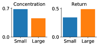
Figure 27: Replay buffer diversity vs. return in the lava environment. On the left we show the concentration of the replay buffer, measured as the percentage of the top-100 high-regret levels that can be produced by just ten parents. On the right we compare the average return on ten-tile test environments. Here, small corresponds to a buffer of size 4k, with no generator, while large indicates a buffer of size 10k, using a generator 10% of the time.

Diversity of the Level Buffer we compare a buffer of size 4k with no DR sampling against our method with a buffer size of 10k and 10% sampling. The plots show the proportion of the top 200 levels produced by just ten initial generator levels, with a significant increase for the smaller buffer. We also compare the performance of the two agents on test levels with ten tiles, showing clear outperformance for the lower concentration agent. It is likely that hyperparameters alone will not be sufficient if we want to scale ACCEL to more open-ended domains, which we leave to future work.

Appendix C Implementation Details

In this section we detail the training procedure for all our experiments. All training runs used a single V100 GPU and Intel Xeon E5-2698 v4 CPUs. Our ACCEL implementation directly builds on top of the Robust PLR codebase, available at https://github.com/facebookresearch/dcd. For PAIRED and Minimax in the maze environment, we report the results from Jiang et al., 2021a .

C.1 Environment Details

Learning with Lava The MiniHack environment is an open-source Gym environment (Brockman et al.,, 2016), which wraps the game of NetHack via the NetHack Learning Environment (Küttler et al.,, 2020). MiniHack allows users (or agents) the ability to fully specify environments leveraging the full NetHack runtime. For our experiments we use a simple $7\times 7$ grid and allow the agent to place lava tiles in any location. The DR agent samples the number of blocks in $[0,20]$. The reward is sparse, with the agent receiving $+1$ reward for reaching the goal and a per timestep penalty of $-0.01$.

Partially-Observable Navigation Each maze consists of a $15\times 15$ grid, where each tile can contain a block, the goal, the agent, or navigable space. The agent receives a reward of $1-T/T_{\textnormal{max}}$ upon reaching the goal, where $T$ is the episode length and $T_{\textnormal{max}}$ is the maximum episode length (set to 250 at training). The agent receives a reward of 0 if it fails to reach the goal.

BipedalWalker We use a modified version of the BipedalWalkerHardcore environment from OpenAI Gym. The agent receives a 24-dimensional proprioceptive state corresponding to inputs from its lidar sensors, angles, and contacts. The agent does not have access to its positional coordinates. The action space is four continuous values that control the torques of its four motors. The environment design space is shown in Table 9, where we show the value of the initial environment parameterization for ACCEL, the edit size, and the maximum values. In this environment, the UED parameters correspond to the ranges of level properties, uniformly sampled to define each level. Thus, combined with a random seed, the UED parameters determine a specific level. Parameters for DR levels are sampled between zero and the maximum value. For PLR, we combine the environment parameterization with the specific seed of the sampled level, ensuring deterministic generation of the replayed level. ACCEL makes each edit by randomly sampling one of the eight environment parameters and adding or subtracting the corresponding edit size listed in Table 9 from the parameter value.

Table 9: Environment design space for the BipedalWalker environment. The UED parameters correspond to the min and max values for each level property. When a specific level is created, each property (i.e. obstacle size) is sampled from the corresponding range.

	Stump Height	Stair Height	Stair Steps	Roughness	Pit Gap
Easy Init	[0,0.4]	[0,0.4]	1	Unif(0, 0.6)	[0,0.8]
Edit Size	0.2	0.2	1	Unif(0, 0.6)	0.4
Max Value	[5,5]	[5,5]	9	10	[10,10]

Table 10: Total number of environment steps for a given number of student PPO updates.

Environment	PPO Updates	PLR	ACCEL
MiniGrid	20k	327M	369M
BipedalWalker	30k	1.96B	2.07B

C.2 Environment Design Procedure

Generating new levels For a fair comparison to the PAIRED level generation procedure, DR is implemented by sampling a uniformly random teacher policy to output actions that set the environment parameters, thereby designing each level. Under PAIRED, this policy is no longer uniformly random, but rather optimized to maximize the estimated regret (e.g. PVL) incurred by the student agent on the resulting levels. The environment design procedure for the lava and maze domains is as follows: For each timestep the teacher receives an observation consisting of a map of the entire level and takes chooses a tile in the grid. For the first $N$ steps, where $N$ is teacher’s budget of blocks (or lava tiles) the teacher always places a block (or lava tile). In the last two time steps, the teacher chooses a location for the goal and agent. This procedure reflects the approach taken in several recent works (Dennis et al.,, 2020; Jiang et al., 2021b, ; Jiang et al., 2021a, ; Khalifa et al.,, 2020). For BipedalWalker, the teacher generates each level by choosing a random value between the minimum value of the “Easy Init” range in Table 9 and the maximum value for each environment parameter. A random integer is then generated to seed the procedural content generation algorithm, which takes the sampled parameters to produce the level.

Editing levels In lava levels, edits only add or remove obstacle tiles (i.e. lava or block tiles), while in MiniGrid mazes, edits can also alter the goal location. If an edit places a lava or block tile in the current goal or agent position, then the new tile replaces the goal or agent, which is randomly relocated after applying all remaining edits.

C.3 Hyperparameters

The majority of our hyperparameters are inherited from previous works such as (Dennis et al.,, 2020; Jiang et al., 2021b, ; Jiang et al., 2021a, ), with a few small changes. For the lava grid in MiniHack we use the agent model from the NetHack paper (Küttler et al.,, 2020), using the glyphs and blstats as observations. The agent has both a global and a locally cropped view (produced using the coordinates in the blstats).

For MiniHack we conduct a grid search across the level replay buffer size $\{4000,10000\}$ for both PLR and ACCEL, and for ACCEL we sweep across the edit method in {random, positive value loss}, where the latter option equates to a learned editor trained with RL to maximize the positive value loss. For MiniGrid we use the replay buffer size from Jiang et al., 2021a and only conduct the ACCEL grid search over the edit objective, again sweeping across {random, positive value loss} and replay rate from {0.8, 0.9}. For MiniGrid, we follow the protocol from Jiang et al., 2021a and select the best hyperparameters using the validation levels {16Rooms, Labyrinth, Maze}. The final hyperparameters chosen are shown in Table 11.

For BipedalWalker we used the continuous control policy from the open source implementation of PPO from Kostrikov, (2018), as well as many of the hyperparameters used in the recommended settings for MuJoCo. This involves a simple feedforward neural network with two hidden layers of size 64 and tanh activations. We tuned the hyperparameters for our base agent using domain randomization, and conducted a sweep over the learning rate {3e-4, 3e-5}, PPO epochs $\{5,20\}$, entropy coefficient {0, 1e-3} and number of minibatches $\{4,32\}$, using the validation performance on BipedalWalkerHardcore. We then used these base agent configurations for all UED algorithms. For PLR we further conducted a sweep over the buffer size $\{1000,5000\}$, replay rate $\{0,9,0.5\}$ and staleness coefficient $\{0.3,0.5,0.7\}$, using the same settings found for both PLR and ACCEL. Finally, for ACCEL we swept over number of edits in {1, 2, 3, 4}.

Table 11: Hyperparameters used for training each method in each environment.

Parameter	MiniHack (Lava)	MiniGrid	BipedalWalker
PPO
$\gamma$	0.995	0.995	0.99
$\lambda_{\text{GAE}}$	0.95	0.95	0.9
PPO rollout length	256	256	2000
PPO epochs	5	5	5
PPO minibatches per epoch	1	1	32
PPO clip range	0.2	0.2	0.2
PPO number of workers	32	32	16
Adam learning rate	1e-4	1e-4	3e-4
Adam $\epsilon$	1e-5	1e-5	1e-5
PPO max gradient norm	0.5	0.5	0.5
PPO value clipping	yes	yes	no
return normalization	no	no	yes
value loss coefficient	0.5	0.5	0.5
student entropy coefficient	0.0	0.0	1e-3
generator entropy coefficient	0.0	0.0	0.0
ACCEL
Edit rate, $q$	1.0	1.0	1.0
Replay rate, $p$	0.9	0.8	0.9
Buffer size, $K$	10000	4000	1000
Scoring function	positive value loss	positive value loss	positive value loss
Edit method	positive value loss	random	random
Number of edits	5	5	3
Prioritization	rank	rank	rank
Temperature, $\beta$	0.3	0.3	0.1
Staleness coefficient, $\rho$	0.3	0.3	0.5
PLR
Scoring function	positive value loss	positive value loss	positive value loss
Replay rate, $p$	0.5	0.5	0.5
Buffer size, $K$	10000	4000	1000

References

- (1) Agarwal, R., Machado, M. C., Castro, P. S., and Bellemare, M. G. (2021a). Contrastive behavioral similarity embeddings for generalization in reinforcement learning. In International Conference on Learning Representations.
- (2) Agarwal, R., Schwarzer, M., Castro, P. S., Courville, A., and Bellemare, M. G. (2021b). Deep reinforcement learning at the edge of the statistical precipice. In Advances in Neural Information Processing Systems.
- Andrychowicz et al., (2017) Andrychowicz, M., Crow, D., Ray, A., Schneider, J., Fong, R., Welinder, P., McGrew, B., Tobin, J., Abbeel, P., and Zaremba, W. (2017). Hindsight experience replay. In Guyon, I., von Luxburg, U., Bengio, S., Wallach, H. M., Fergus, R., Vishwanathan, S. V. N., and Garnett, R., editors, Advances in Neural Information Processing Systems 30.
- Andrychowicz et al., (2020) Andrychowicz, O. M., Baker, B., Chociej, M., Józefowicz, R., McGrew, B., Pachocki, J., Petron, A., Plappert, M., Powell, G., Ray, A., Schneider, J., Sidor, S., Tobin, J., Welinder, P., Weng, L., and Zaremba, W. (2020). Learning dexterous in-hand manipulation. The International Journal of Robotics Research, 39(1):3–20.
- Ball et al., (2021) Ball, P. J., Lu, C., Parker-Holder, J., and Roberts, S. J. (2021). Augmented world models facilitate zero-shot dynamics generalization from a single offline environment. In The International Conference on Machine Learning.
- Baranes and Oudeyer, (2009) Baranes, A. and Oudeyer, P.-Y. (2009). Robust intrinsically motivated exploration and active learning. pages 1 – 6.
- Berner et al., (2019) Berner, C., Brockman, G., Chan, B., Cheung, V., Debiak, P., Dennison, C., Farhi, D., Fischer, Q., Hashme, S., Hesse, C., Józefowicz, R., Gray, S., Olsson, C., Pachocki, J., Petrov, M., de Oliveira Pinto, H. P., Raiman, J., Salimans, T., Schlatter, J., Schneider, J., Sidor, S., Sutskever, I., Tang, J., Wolski, F., and Zhang, S. (2019). Dota 2 with large scale deep reinforcement learning. CoRR, abs/1912.06680.
- Berthouze and Lungarella, (2004) Berthouze, L. and Lungarella, M. (2004). Motor skill acquisition under environmental perturbations: On the necessity of alternate freezing and freeing of degrees of freedom. Adapt. Behav., 12(1):47–64.
- Bhaumik et al., (2020) Bhaumik, D., Khalifa, A., Green, M. C., and Togelius, J. (2020). Tree search versus optimization approaches for map generation. In AAAI 2020.
- Brant and Stanley, (2017) Brant, J. C. and Stanley, K. O. (2017). Minimal criterion coevolution: A new approach to open-ended search. In Proceedings of the Genetic and Evolutionary Computation Conference, GECCO ’17, page 67–74, New York, NY, USA. Association for Computing Machinery.
- Brockman et al., (2016) Brockman, G., Cheung, V., Pettersson, L., Schneider, J., Schulman, J., Tang, J., and Zaremba, W. (2016). OpenAI Gym.
- Campero et al., (2021) Campero, A., Raileanu, R., Kuttler, H., Tenenbaum, J. B., Rocktäschel, T., and Grefenstette, E. (2021). Learning with AMIGo: Adversarially motivated intrinsic goals. In International Conference on Learning Representations.
- Chevalier-Boisvert et al., (2018) Chevalier-Boisvert, M., Willems, L., and Pal, S. (2018). Minimalistic gridworld environment for OpenAI Gym. https://github.com/maximecb/gym-minigrid.
- Cobbe et al., (2020) Cobbe, K., Hesse, C., Hilton, J., and Schulman, J. (2020). Leveraging procedural generation to benchmark reinforcement learning. In Proceedings of the 37th International Conference on Machine Learning, pages 2048–2056.
- Dennis et al., (2020) Dennis, M., Jaques, N., Vinitsky, E., Bayen, A., Russell, S., Critch, A., and Levine, S. (2020). Emergent complexity and zero-shot transfer via unsupervised environment design. In Advances in Neural Information Processing Systems, volume 33.
- Dharna et al., (2020) Dharna, A., Togelius, J., and Soros, L. B. (2020). Co-generation of game levels and game-playing agents. Proceedings of the AAAI Conference on Artificial Intelligence and Interactive Digital Entertainment, 16(1):203–209.
- (17) Earle, S., Edwards, M., Khalifa, A., Bontrager, P., and Togelius, J. (2021a). Learning controllable content generators. In IEEE Conference on Games (CoG).
- (18) Earle, S., Snider, J., Fontaine, M. C., Nikolaidis, S., and Togelius, J. (2021b). Illuminating diverse neural cellular automata for level generation.
- Eimer et al., (2021) Eimer, T., Biedenkapp, A., Hutter, F., and Lindauer, M. (2021). Self-paced context evaluation for contextual reinforcement learning. In The International Conference on Machine Learning.
- Everett et al., (2019) Everett, R., Cobb, A., Markham, A., and Roberts, S. (2019). Optimising worlds to evaluate and influence reinforcement learning agents. In Proceedings of the 18th International Conference on Autonomous Agents and MultiAgent Systems, AAMAS ’19.
- Fang et al., (2021) Fang, K., Zhu, Y., Savarese, S., and Li, F.-F. (2021). Adaptive procedural task generation for hard-exploration problems. In International Conference on Learning Representations.
- Florensa et al., (2018) Florensa, C., Held, D., Geng, X., and Abbeel, P. (2018). Automatic goal generation for reinforcement learning agents. In Dy, J. and Krause, A., editors, Proceedings of the 35th International Conference on Machine Learning, volume 80 of Proceedings of Machine Learning Research, pages 1515–1528. PMLR.
- Florensa et al., (2017) Florensa, C., Held, D., Wulfmeier, M., Zhang, M., and Abbeel, P. (2017). Reverse curriculum generation for reinforcement learning. In 1st Annual Conference on Robot Learning, CoRL 2017, Mountain View, California, USA, November 13-15, 2017, Proceedings, volume 78 of Proceedings of Machine Learning Research, pages 482–495. PMLR.
- Fontaine et al., (2021) Fontaine, M. C., Hsu, Y., Zhang, Y., Tjanaka, B., and Nikolaidis, S. (2021). On the importance of environments in human-robot coordination. In Shell, D. A., Toussaint, M., and Hsieh, M. A., editors, Robotics: Science and Systems XVII, Virtual Event, July 12-16, 2021.
- Gajewski et al., (2019) Gajewski, A., Clune, J., Stanley, K. O., and Lehman, J. (2019). Evolvability ES: Scalable and direct optimization of evolvability. In Proceedings of the Genetic and Evolutionary Computation Conference, GECCO ’19, pages 107–115, New York, NY, USA. ACM.
- Ghosh et al., (2021) Ghosh, D., Rahme, J., Kumar, A., Zhang, A., Adams, R. P., and Levine, S. (2021). Why generalization in rl is difficult: Epistemic pomdps and implicit partial observability. arXiv preprint arXiv:2107.06277.
- Gur et al., (2021) Gur, I., Jaques, N., Malta, K., Tiwari, M., Lee, H., and Faust, A. (2021). Adversarial environment generation for learning to navigate the web.
- Hu and Foerster, (2020) Hu, H. and Foerster, J. N. (2020). Simplified action decoder for deep multi-agent reinforcement learning. In 8th International Conference on Learning Representations, ICLR 2020, Addis Ababa, Ethiopia, April 26-30, 2020. OpenReview.net.
- Igl et al., (2019) Igl, M., Ciosek, K., Li, Y., Tschiatschek, S., Zhang, C., Devlin, S., and Hofmann, K. (2019). Generalization in reinforcement learning with selective noise injection and information bottleneck. In Advances in Neural Information Processing Systems.
- Jakobi, (1997) Jakobi, N. (1997). Evolutionary robotics and the radical envelope-of-noise hypothesis. Adaptive Behavior, 6(2):325–368.
- James et al., (2017) James, S., Davison, A. J., and Johns, E. (2017). Transferring end-to-end visuomotor control from simulation to real world for a multi-stage task. In 1st Conference on Robot Learning.
- (32) Jiang, M., Dennis, M., Parker-Holder, J., Foerster, J., Grefenstette, E., and Rocktäschel, T. (2021a). Replay-guided adversarial environment design. In Advances in Neural Information Processing Systems.
- (33) Jiang, M., Grefenstette, E., and Rocktäschel, T. (2021b). Prioritized level replay. In The International Conference on Machine Learning.
- Juliani et al., (2019) Juliani, A., Khalifa, A., Berges, V., Harper, J., Teng, E., Henry, H., Crespi, A., Togelius, J., and Lange, D. (2019). Obstacle Tower: A Generalization Challenge in Vision, Control, and Planning. In IJCAI.
- Justesen et al., (2018) Justesen, N., Torrado, R. R., Bontrager, P., Khalifa, A., Togelius, J., and Risi, S. (2018). Procedural level generation improves generality of deep reinforcement learning. CoRR, abs/1806.10729.
- Keren et al., (2017) Keren, S., Pineda, L., Gal, A., Karpas, E., and Zilberstein, S. (2017). Equi-reward utility maximizing design in stochastic environments. In Proceedings of the International Conference on Automated Planning and Scheduling.
- Keren et al., (2019) Keren, S., Pineda, L., Gal, A., Karpas, E., and Zilberstein, S. (2019). Efficient heuristic search for optimal environment redesign. In Proceedings of the International Conference on Automated Planning and Scheduling, volume 29, pages 246–254.
- Khalifa et al., (2020) Khalifa, A., Bontrager, P., Earle, S., and Togelius, J. (2020). Pcgrl: Procedural content generation via reinforcement learning. Proceedings of the AAAI Conference on Artificial Intelligence and Interactive Digital Entertainment, 16(1):95–101.
- Kirk et al., (2021) Kirk, R., Zhang, A., Grefenstette, E., and Rocktäschel, T. (2021). A survey of generalisation in deep reinforcement learning. CoRR, abs/2111.09794.
- Klink et al., (2019) Klink, P., Abdulsamad, H., Belousov, B., and Peters, J. (2019). Self-paced contextual reinforcement learning. In Conference on Robot Learning.
- Kostrikov, (2018) Kostrikov, I. (2018). Pytorch implementations of reinforcement learning algorithms. https://github.com/ikostrikov/pytorch-a2c-ppo-acktr-gail.
- Kostrikov et al., (2021) Kostrikov, I., Yarats, D., and Fergus, R. (2021). Image augmentation is all you need: Regularizing deep reinforcement learning from pixels. In International Conference on Learning Representations.
- Küttler et al., (2020) Küttler, H., Nardelli, N., Miller, A. H., Raileanu, R., Selvatici, M., Grefenstette, E., and Rocktäschel, T. (2020). The NetHack Learning Environment. In Proceedings of the Conference on Neural Information Processing Systems (NeurIPS).
- Laskin et al., (2020) Laskin, M., Lee, K., Stooke, A., Pinto, L., Abbeel, P., and Srinivas, A. (2020). Reinforcement learming with augmented data. In Advances in Neural Information Processing Systems 33.
- Lehman and Miikkulainen, (2015) Lehman, J. and Miikkulainen, R. (2015). Extinction events can accelerate evolution. PloS one, 10(8):e0132886.
- Liu et al., (2021) Liu, J., Snodgrass, S., Khalifa, A., Risi, S., Yannakakis, G. N., and Togelius, J. (2021). Deep learning for procedural content generation. Neural Comput. Appl., 33(1):19–37.
- Matiisen et al., (2020) Matiisen, T., Oliver, A., Cohen, T., and Schulman, J. (2020). Teacher-student curriculum learning. IEEE Trans. Neural Networks Learn. Syst., 31(9):3732–3740.
- Mazumdar et al., (2020) Mazumdar, E., Ratliff, L. J., and Sastry, S. S. (2020). On gradient-based learning in continuous games. SIAM J. Math. Data Sci., 2(1):103–131.
- Mehta et al., (2020) Mehta, B., Diaz, M., Golemo, F., Pal, C. J., and Paull, L. (2020). Active domain randomization. In Proceedings of the Conference on Robot Learning.
- Mendonca et al., (2021) Mendonca, R., Rybkin, O., Daniilidis, K., Hafner, D., and Pathak, D. (2021). Discovering and achieving goals via world models.
- Mnih et al., (2013) Mnih, V., Kavukcuoglu, K., Silver, D., Graves, A., Antonoglou, I., Wierstra, D., and Riedmiller, M. A. (2013). Playing atari with deep reinforcement learning. ArXiv, abs/1312.5602.
- Modi et al., (2017) Modi, A., Jiang, N., Singh, S., and Tewari, A. (2017). Markov decision processes with continuous side information. In Algorithmic Learning Theory.
- OpenAI et al., (2019) OpenAI, Akkaya, I., Andrychowicz, M., Chociej, M., Litwin, M., McGrew, B., Petron, A., Paino, A., Plappert, M., Powell, G., Ribas, R., Schneider, J., Tezak, N., Tworek, J., Welinder, P., Weng, L., Yuan, Q., Zaremba, W., and Zhang, L. (2019). Solving rubik’s cube with a robot hand. CoRR, abs/1910.07113.
- OpenAI et al., (2021) OpenAI, O., Plappert, M., Sampedro, R., Xu, T., Akkaya, I., Kosaraju, V., Welinder, P., D’Sa, R., Petron, A., de Oliveira Pinto, H. P., Paino, A., Noh, H., Weng, L., Yuan, Q., Chu, C., and Zaremba, W. (2021). Asymmetric self-play for automatic goal discovery in robotic manipulation.
- Packer et al., (2019) Packer, C., Gao, K., Kos, J., Krahenbuhl, P., Koltun, V., and Song, D. (2019). Assessing generalization in deep reinforcement learning.
- Parker-Holder et al., (2022) Parker-Holder, J., Rajan, R., Song, X., Biedenkapp, A., Miao, Y., Eimer, T., Zhang, B., Nguyen, V., Calandra, R., Faust, A., Hutter, F., and Lindauer, M. (2022). Automated reinforcement learning (autorl): A survey and open problems. CoRR, abs/2201.03916.
- Peng et al., (2017) Peng, X. B., Andrychowicz, M., Zaremba, W., and Abbeel, P. (2017). Sim-to-real transfer of robotic control with dynamics randomization. CoRR, abs/1710.06537.
- Perez-Liebana et al., (2019) Perez-Liebana, D., Liu, J., Khalifa, A., Gaina, R. D., Togelius, J., and Lucas, S. M. (2019). General video game ai: A multitrack framework for evaluating agents, games, and content generation algorithms. IEEE Transactions on Games, 11(3):195–214.
- Pinto et al., (2017) Pinto, L., Davidson, J., and Gupta, A. (2017). Supervision via competition: Robot adversaries for learning tasks. In 2017 IEEE International Conference on Robotics and Automation (ICRA), pages 1601–1608.
- Pong et al., (2020) Pong, V., Dalal, M., Lin, S., Nair, A., Bahl, S., and Levine, S. (2020). Skew-fit: State-covering self-supervised reinforcement learning. In Proceedings of the 37th International Conference on Machine Learning, pages 7783–7792.
- Portelas et al., (2019) Portelas, R., Colas, C., Hofmann, K., and Oudeyer, P. (2019). Teacher algorithms for curriculum learning of deep RL in continuously parameterized environments. In Kaelbling, L. P., Kragic, D., and Sugiura, K., editors, 3rd Annual Conference on Robot Learning, CoRL 2019, Osaka, Japan, October 30 - November 1, 2019, Proceedings, volume 100 of Proceedings of Machine Learning Research, pages 835–853. PMLR.
- Portelas et al., (2020) Portelas, R., Colas, C., Weng, L., Hofmann, K., and Oudeyer, P.-Y. (2020). Automatic curriculum learning for deep rl: A short survey. arXiv preprint arXiv:2003.04664.
- Pugh et al., (2016) Pugh, J. K., Soros, L. B., and Stanley, K. O. (2016). Quality diversity: A new frontier for evolutionary computation. Frontiers in Robotics and AI, 3:40.
- Racaniere et al., (2020) Racaniere, S., Lampinen, A., Santoro, A., Reichert, D., Firoiu, V., and Lillicrap, T. (2020). Automated curriculum generation through setter-solver interactions. In International Conference on Learning Representations.
- Raileanu et al., (2021) Raileanu, R., Goldstein, M., Yarats, D., Kostrikov, I., and Fergus, R. (2021). Automatic data augmentation for generalization in deep reinforcement learning. In Advances in Neural Information Processing Systems.
- Raparthy et al., (2020) Raparthy, S. C., Mehta, B., Golemo, F., and Paull, L. (2020). Generating automatic curricula via self-supervised active domain randomization. CoRR, abs/2002.07911.
- Raup, (1986) Raup, D. M. (1986). Biological extinction in earth history. Science, 231(4745):1528–1533.
- Risi and Togelius, (2020) Risi, S. and Togelius, J. (2020). Increasing generality in machine learning through procedural content generation. Nature Machine Intelligence, 2.
- Sadeghi and Levine, (2017) Sadeghi, F. and Levine, S. (2017). CAD2RL: real single-image flight without a single real image. In Amato, N. M., Srinivasa, S. S., Ayanian, N., and Kuindersma, S., editors, Robotics: Science and Systems XIII, Massachusetts Institute of Technology, Cambridge, Massachusetts, USA, July 12-16, 2017.
- Samvelyan et al., (2021) Samvelyan, M., Kirk, R., Kurin, V., Parker-Holder, J., Jiang, M., Hambro, E., Petroni, F., Kuttler, H., Grefenstette, E., and Rocktäschel, T. (2021). Minihack the planet: A sandbox for open-ended reinforcement learning research. In Thirty-fifth Conference on Neural Information Processing Systems Datasets and Benchmarks Track.
- Savage, (1951) Savage, L. J. (1951). The theory of statistical decision. Journal of the American Statistical association.
- Schmidhuber, (2013) Schmidhuber, J. (2013). Powerplay: Training an increasingly general problem solver by continually searching for the simplest still unsolvable problem. Frontiers in Psychology, 4:313.
- Schulman et al., (2016) Schulman, J., Moritz, P., Levine, S., Jordan, M., and Abbeel, P. (2016). High-dimensional continuous control using generalized advantage estimation. In Proceedings of the International Conference on Learning Representations (ICLR).
- Schulman et al., (2018) Schulman, J., Wolski, F., Dhariwal, P., Radford, A., and Klimov, O. (2016-2018). Proximal policy optimization algorithms. arXiv preprint arXiv:1707.06347.
- Silver et al., (2016) Silver, D., Huang, A., Maddison, C. J., Guez, A., Sifre, L., van den Driessche, G., Schrittwieser, J., Antonoglou, I., Panneershelvam, V., Lanctot, M., Dieleman, S., Grewe, D., Nham, J., Kalchbrenner, N., Sutskever, I., Lillicrap, T. P., Leach, M., Kavukcuoglu, K., Graepel, T., and Hassabis, D. (2016). Mastering the game of Go with deep neural networks and tree search. Nature, 529:484–489.
- Silver et al., (2021) Silver, D., Singh, S., Precup, D., and Sutton, R. S. (2021). Reward is enough. Artificial Intelligence, 299:103535.
- Song et al., (2020) Song, X., Jiang, Y., Tu, S., Du, Y., and Neyshabur, B. (2020). Observational overfitting in reinforcement learning. In 8th International Conference on Learning Representations, ICLR 2020, Addis Ababa, Ethiopia, April 26-30, 2020. OpenReview.net.
- Soros and Stanley, (2014) Soros, L. and Stanley, K. (2014). Identifying necessary conditions for open-ended evolution through the artificial life world of chromaria. Artificial Life Conference Proceedings, (26):793–800.
- Stanley et al., (2019) Stanley, K., Clune, J., Lehman, J., and Miikkulainen, R. (2019). Designing neural networks through neuroevolution. Nature Machine Intelligence, 1.
- Stanley et al., (2017) Stanley, K. O., Lehman, J., and Soros, L. (2017). Open-endedness: The last grand challenge you’ve never heard of. While open-endedness could be a force for discovering intelligence, it could also be a component of AI itself.
- Sturtevant et al., (2020) Sturtevant, N., Decroocq, N., Tripodi, A., and Guzdial, M. (2020). The unexpected consequence of incremental design changes. In Proceedings of the AAAI Conference on Artificial Intelligence and Interactive Digital Entertainment, volume 16, pages 130–136.
- Sukhbaatar et al., (2018) Sukhbaatar, S., Lin, Z., Kostrikov, I., Synnaeve, G., Szlam, A., and Fergus, R. (2018). Intrinsic motivation and automatic curricula via asymmetric self-play. In International Conference on Learning Representations.
- Summerville et al., (2018) Summerville, A., Snodgrass, S., Guzdial, M., Holmgård, C., Hoover, A. K., Isaksen, A., Nealen, A., and Togelius, J. (2018). Procedural content generation via machine learning (PCGML). IEEE Trans. Games, 10(3):257–270.
- Sutton and Barto, (1998) Sutton, R. S. and Barto, A. G. (1998). Introduction to Reinforcement Learning. MIT Press, Cambridge, MA, USA, 1st edition.
- Team et al., (2021) Team, O. E. L., Stooke, A., Mahajan, A., Barros, C., Deck, C., Bauer, J., Sygnowski, J., Trebacz, M., Jaderberg, M., Mathieu, M., McAleese, N., Bradley-Schmieg, N., Wong, N., Porcel, N., Raileanu, R., Hughes-Fitt, S., Dalibard, V., and Czarnecki, W. M. (2021). Open-ended learning leads to generally capable agents. CoRR, abs/2107.12808.
- Tobin et al., (2017) Tobin, J., Fong, R., Ray, A., Schneider, J., Zaremba, W., and Abbeel, P. (2017). Domain randomization for transferring deep neural networks from simulation to the real world. In 2017 IEEE/RSJ International Conference on Intelligent Robots and Systems, IROS 2017, Vancouver, BC, Canada, September 24-28, 2017, pages 23–30. IEEE.
- Togelius and Schmidhuber, (2008) Togelius, J. and Schmidhuber, J. (2008). An experiment in automatic game design. In 2008 IEEE Symposium On Computational Intelligence and Games, pages 111–118.
- Vinyals et al., (2019) Vinyals, O., Babuschkin, I., Czarnecki, W. M., Mathieu, M., Dudzik, A., Chung, J., Choi, D. H., Powell, R., Ewalds, T., Georgiev, P., Oh, J., Horgan, D., Kroiss, M., Danihelka, I., Huang, A., Sifre, L., Cai, T., Agapiou, J. P., Jaderberg, M., Vezhnevets, A. S., Leblond, R., Pohlen, T., Dalibard, V., Budden, D., Sulsky, Y., Molloy, J., Paine, T. L., Gülçehre, Ç., Wang, Z., Pfaff, T., Wu, Y., Ring, R., Yogatama, D., Wünsch, D., McKinney, K., Smith, O., Schaul, T., Lillicrap, T. P., Kavukcuoglu, K., Hassabis, D., Apps, C., and Silver, D. (2019). Grandmaster level in starcraft II using multi-agent reinforcement learning. Nat., 575(7782):350–354.
- Wang et al., (2019) Wang, R., Lehman, J., Clune, J., and Stanley, K. O. (2019). Paired open-ended trailblazer (POET): endlessly generating increasingly complex and diverse learning environments and their solutions. CoRR, abs/1901.01753.
- Wang et al., (2020) Wang, R., Lehman, J., Rawal, A., Zhi, J., Li, Y., Clune, J., and Stanley, K. (2020). Enhanced POET: Open-ended reinforcement learning through unbounded invention of learning challenges and their solutions. In III, H. D. and Singh, A., editors, Proceedings of the 37th International Conference on Machine Learning, volume 119 of Proceedings of Machine Learning Research, pages 9940–9951. PMLR.
- Whiteson et al., (2009) Whiteson, S., Tanner, B., Taylor, M. E., and Stone, P. (2009). Generalized domains for empirical evaluations in reinforcement learning.
- (92) Zhang, A., Ballas, N., and Pineau, J. (2018a). A dissection of overfitting and generalization in continuous reinforcement learning. CoRR, abs/1806.07937.
- (93) Zhang, C., Vinyals, O., Munos, R., and Bengio, S. (2018b). A study on overfitting in deep reinforcement learning. CoRR, abs/1804.06893.
- Zhang et al., (2009) Zhang, H., Chen, Y., and Parkes, D. (2009). A general approach to environment design with one agent. In Proceedings of the 21st International Jont Conference on Artifical Intelligence, IJCAI’09, page 2002–2008.
- Zhang and Parkes, (2008) Zhang, H. and Parkes, D. (2008). Value-based policy teaching with active indirect elicitation. In Proceedings of the 23rd National Conference on Artificial Intelligence - Volume 1, AAAI’08, page 208–214. AAAI Press.
- Zhang et al., (2020) Zhang, Y., Abbeel, P., and Pinto, L. (2020). Automatic curriculum learning through value disagreement. In Larochelle, H., Ranzato, M., Hadsell, R., Balcan, M. F., and Lin, H., editors, Advances in Neural Information Processing Systems, volume 33, pages 7648–7659. Curran Associates, Inc.