py-irt: A Scalable Item Response Theory Library for Python

Abstract

py-irt is a Python library for fitting Bayesian Item Response Theory (irt) models. py-irt estimates latent traits of subjects and items, making it appropriate for use in IRT tasks as well as ideal-point models. py-irt is built on top of the Pyro and PyTorch frameworks and uses gpu-accelerated training to scale to large data sets. Code, documentation, and examples can be found at https://github.com/nd-ball/py-irt. py-irt can be installed from the GitHub page or the Python Package Index (PyPI).

1 Introduction

Item Response Theory (irt) models jointly estimate latent traits of items (e.g., the difficulty of exam questions) and subjects (e.g., the ability of human test-takers). Originally developed as an alternative to simple summary statistics (Edgeworth 1888), irt sees widespread use in education testing (Lord et al. 1968) for scale construction and evaluation (Carlson and von Davier 2013). Increasingly, it is also being used to evaluate machine learning models (Lalor 2020).

Research using irt spans fields such as educational testing, machine learning, management, operations, and policital science. Recent work on irt in machine learning investigates its use for model and data analysis (Martínez-Plumed et al. 2016, 2019, Vania et al. 2021), test set evaluation (Lalor et al. 2016, Rodriguez et al. 2021), deep neural network training and behavior (Lalor et al. 2019, Lalor and Yu 2020), and chatbot data evaluation (Sedoc and Ungar 2020).

There is also a stream of work in the business community that leverages irt models, including near-miss analyses (Cui et al. 2017), scale construction in marketing (de Jong et al. 2009, 2012), and probability forecasting (Satopää et al. 2021). Researchers in operations use irt for machine learning model comparison (Roy et al. 2019).

irt models are known as ideal-point models in political science literature (Gerrish and Blei 2011, Poole and Rosenthal 2017). In this context, the models are used to estimate latent party affiliation for politicians based on binary voting records (e.g., voting for or against a proposed bill). Extensions to ideal point models incorporate the text of the bills and politicians’ speeches as well (Nguyen et al. 2015).

Existing libraries for fitting irt models are implemented in R and cannot scale to large-scale data. There is a need for a fast, user-friendly irt library. We present py-irt, a Python package for fitting Bayesian irt models. py-irt is built on top of the Pyro probabilistic programming language (Bingham et al. 2019), which itself makes use of PyTorch gpu-accelerated tensor math and automatic differentiation (Paszke et al. 2019). Models are learned via stochastic variational inference (Kingma and Welling 2013) and mini-batch gradient descent, making them scalable to large data sets.

In this work, we describe the development of py-irt, describe the code and its functionality, and demonstrate applications in natural language processing (nlp) and computer vision (cv). We demonstrate that py-irt is an easy-to-use and efficient library for developing irt models.

2 Background

In this section, we introduce notation for irt models and describe a class of irt models for binary data. We then demonstrate two methods for estimating irt model parameters: marginal maximum likelihood estimation and variational inference. Finally, we highlight existing packages for fitting irt models.

2.1 Notation

irt is a widely used (van Rijn et al. 2016) psychometric methodology for learning latent parameters of items and subjects (Baker 2001, Baker and Kim 2004). Typically, subjects are human test-takers, and items are assessment questions (e.g., from a standardized test, de Jong et al. 2009, 2012). For dichotomous data, a subject’s responses to a set of items are graded as correct or incorrect. The binary response matrix of multiple subjects’ responses is used to estimate latent parameters of the items and the latent ability of the subjects. irt models learn these latent parameters from the input response pattern matrix $\mathbf{Z}^{I\times J}$, where each row in the matrix represents subject $j^{\prime}s$ responses to the items in the dataset:

$$Z^{j}=[\mathbf{I}[\hat{y}^{j}_{0}=y_{0}],\dots,\mathbb{I}[\hat{y}^{j}_{I}=y_{I}]]$$ (1)

where $\mathbb{I}$ is the indicator function, and is equal to $1$ when the expression is true and $0$ when the expression is false. Put another way, $\mathbf{Z}$ is a binarized, graded representation of the subjects’ responses to the items.

2.2 IRT Models

We next describe several variations of irt models that are implemented in py-irt.

The one-parameter logistic model (1PL), also known as the Rasch model, estimates a latent ability parameter $\theta_{j}$ for subjects and a latent difficulty parameter $b_{i}$ for items (Equation 2).

$$p(y_{ij}=1|b_{i},\theta_{j})=\frac{1}{1+e^{-(\theta_{j}-b_{i})}}$$ (2)

Equation 2 defines an Item Characteristic Curve (iccs) for a particular item (Figure 1). For a particular subject, the probability of correctly answering a given item is a function of the subject’s latent ability and the item’s latent characteristics. For individuals of higher ability, the probability of correctly answering an item increases—all else equal.

More complex irt models estimate additional latent parameters for the items. The two-parameter logistic (2PL) model adds a discrimination parameter $a_{i}$, so that different items have steeper or shallower slopes at the steepest point (Equation 3). The three-parameter logistic (3PL) model adds a guessing parameter ($c_{i}$) to model the fact that, even at low levels of subject ability, there is a non-zero probability that a subject will guess a question’s answer correctly (Equation 4). The feasibility model of Rodriguez et al. (2021) sets an upper bound on the icc for “unanswerable” questions (Equation 5). These models can also be multidimensional in the latent space (Reckase 2009).

$$p(y_{ij}=1|a_{i},b_{i},\theta_{j}) =\frac{1}{1+e^{-a_{i}(\theta_{j}-b_{i})}}$$ (3)

$$p(y_{ij}=1|a_{i},b_{i},c_{i},\theta_{j}) =c_{i}+\frac{1-c_{i}}{1+e^{-a_{i}(\theta_{j}-b_{i})}}$$ (4)

$$p(y_{ij}=1|a_{i},b_{i},\lambda_{i},\theta_{j}) =\frac{\lambda_{i}}{1+e^{-a_{i}(\theta_{j}-b_{i})}}$$ (5)

(a)

(b)

(c)

Figure 1: 1(a): ICCs for an easy item (solid) and a hard item (dashed). Vertical lines indicate the point on the ability scale where $p(y_{ij}=1|b_{i},\theta_{j})=0.5$. 1(b): ICCs where the discrimination parameter ($a_{i}$) varies. 1(c): ICCs where the guessing parameter ($c_{i}$) varies.

2.3 Parameter Estimation

To derive model parameters, we use probabilistic inference (Pearl 1988) to find the latent subject and item parameters that best explain the data—in this case the response pattern matrix $\mathbf{Z}$. The likelihood of a particular response matrix given latent subject and item parameters is:

$$p(\mathbf{Z}|\Theta,B)=\prod_{j=1}^{J}\prod_{i=1}^{I}p(\mathbf{Z}_{ij}=y_{ij}|\theta_{j},b_{i}).$$ (6)

For computational efficiency, this is often represented in log space:

$$\log p(\mathbf{Z}|\Theta,B)=\sum_{j=1}^{J}\sum_{i=1}^{I}\log p(\mathbf{Z}_{ij}=y_{ij}|\theta_{j},b_{i}).$$ (7)

Traditionally, this is fit using marginal maximum likelihood estimation. Bock and Aitkin (1981) proposed an expectation-maximization algorithm, where ability is integrated out, and at each time step $t$ the item parameters are estimated using maximum a posteriori (MAP) estimation:

E step: $$p(z_{ij}|b_{i}^{t})=\int_{\theta_{i}}p(z_{ij}|\theta_{j},b_{i}^{t})p(\theta_{j})d\theta_{j}$$ (8)

M step: $$b_{i}^{t+1}=\arg\max_{b_{i}}\sum_{i}^{I}\log p(z_{ij}|b_{i}^{t})$$ (9)

Once item parameter estimation is complete, estimating subject ability is also done via MAP estimation.

Marginal maximum likelihood estimation does not scale well to large data sets or a large number of subjects. As an alternative, some have proposed Bayesian methods to account both for scaling and also to allow for uncertainty estimation (Natesan et al. 2016). The Bayesian approach attempts to estimate the latent parameters given the response pattern data:

$$p(\Theta,B|\mathbf{Z})$$ (10)

Because calculating this posterior is intractable, approximate inference techniques such as variational inference are used instead (Jordan et al. 1998).

Recent work has investigated using variational inference (vi) (Natesan et al. 2016). vi estimates a distribution over the latent variables that approximates the true posterior and considers mean and variance estimates for calculating uncertainty. Means for the variational parameters are drawn from Normal distributions, and scale parameters are drawn from Gamma distributions (Lalor et al. 2019).

$$q_{\phi}(\theta,b,\mu,\tau)=q(\mu)q(\tau)\prod_{i,j}q(\theta_{j})q(b_{i})$$ (11)

Now the optimization task is to identify the variational parameters that minimize the kl Divergence ($D_{\text{KL}}$) with the true (unknown) posterior:

$$q_{\phi^{*}}(\theta,b,\mu,\tau)=\arg\min_{q_{\phi}}D_{\text{KL}}(q_{\phi}(\theta,b,\mu,\tau)||p(\theta,b|\mathbf{Z}))$$ (12)

2.4 Related Libraries

Most irt-related software packages are implemented in R and target human-sized data, where the number of subjects and items is relatively small. However, when applying irt models to machine learning-scale problems (e.g., an ensemble of neural network models trained on the 50,000 cifar training examples, Krizhevsky et al. 2009), many existing irt programs are not able to scale despite work showing that vi makes this possible (Wu et al. 2020). For researchers working in Python with machine learning libraries such as Tensorflow (Abadi et al. 2016) or PyTorch (Paszke et al. 2019, Zhang et al. 2021), moving from Python to R to incorporate irt analysis is not ideal. To the best of our knowledge, there is no existing resource for the research community to fit large irt models in Python, particularly Bayesian irt models that allow for estimating uncertainty in parameter estimation.

Existing packages for fitting irt models include mirt (Chalmers et al. 2015), ltm (Rizopoulos 2006), and equateIRT (Battauz 2015) in R. irt models can also be fit in Python using Stan (Carpenter et al. 2017), but this requires users to write down their model using the Stan configuration and due to its use of Markov Chain Monte Carlo methods (Kim and Bolt 2007) takes substantially longer to run. There is a need for a user-friendly irt library in Python, particularly for users in the wider research community who may want to easily plug difficulty and ability estimation into a larger (typically Pythonic) data science pipeline.

py-irt has several benefits: 1) as a high-level Python package, users can easily fit irt models for their data sets, 2) py-irt can be used as a command-line interface (CLI) or Python module for flexibility, 3) py-irt’s Bayesian implementation allows for uncertainty in output via latent trait means and variances, and 4) by leveraging pyro’s PyTorch backend, large-scale models can be fit efficiently via gpu acceleration. The scalability and ease of use make py-irt beneficial for researchers looking to implement larger models with larger data sets of items and subjects.

3 Implementation

We next describe how py-irt is implemented and demonstrate how researchers can fit irt models and define new irt models in py-irt. py-irt is implemented in Python and built using Pyro, a probabilistic programming language (Bingham et al. 2019). Pyro allows for the flexible creation of Bayesian models. To achieve scalability, it uses a PyTorch (Paszke et al. 2019) backend. Pyro implements several inference algorithms, such as nuts (Hoffman et al. 2014) and stochastic variational inference (Kingma and Welling 2013).

3.1 Fitting Models

For practitioners, py-irt can be used as either a command-line interface (CLI) or a Python module. To run py-irt, users first format their response pattern dataset into the py-irt jsonlines format (Figure 2(a)). Each row in the data represents a different subject. Each subject has a unique id, and a dictionary of responses ($1$ or $0$) for uniquely identified items. This maintains readability of the dataset while still allowing for sparse response patterns.

⬇

1{

2 "subject_id": "pedro",

3 "responses": {

4 "q1": 1,

5 "q2": 0,

6 "q3": 1,

7 "q4": 0

8 }

9}

10{

11 "subject_id": "pinguino",

12 "responses": {

13 "q1": 1,

14 "q2": 1,

15 "q3": 0,

16 "q4": 0

17 }

18}

19{

20 "subject_id": "ken",

21 "responses": {

22 "q1": 1,

23 "q2": 1,

24 "q3": 1,

25 "q4": 1

26 }

27}

28{

29 "subject_id": "burt",

30 "responses": {

31 "q1": 0,

32 "q2": 0,

33 "q3": 0,

34 "q4": 0

35 }

36}

(a)

⬇

1{

2 "ability": [

3 -1.9317363500595093,

4 1.364127278327942,

5 -0.04978247731924057,

6 -0.2984223961830139

7 ],

8 "diff": [

9 -0.31013718247413635,

10 5.723265171051025,

11 0.7128681540489197,

12 -4.38165283203125

13 ],

14 "irt_model": "1pl",

15 "item_ids": {

16 "0": "q3",

17 "1": "q4",

18 "2": "q2",

19 "3": "q1"

20 },

21 "subject_ids": {

22 "0": "burt",

23 "1": "ken",

24 "2": "pinguino",

25 "3": "pedro"

26 }

27}

(b)

Figure 2: An example of the py-irt input data format (2(a)) and the py-irt output for a 1PL model (2(b)).

To fit a 1PL model from the command line, users execute a single command (Figure 3). The output is a json dictionary containing estimated item and subject parameters. Since subject and item identifiers are not tied to their positions in the model, the output file also links the position of parameters and ids (Figure 2(b)).

⬇

1 py-irt train 1pl data/data.jsonlines output/1pl/

Figure 3: Command line function for training a py-irt model.

3.2 Defining Models

Researchers can define their own irt models using py-irt. In the Pyro tradition, py-irt implements models using the model-guide paradigm. The probabilistic model is specified, and variational guide distributions are initialized (Figure 5).

⬇

1 @abstract_model.IrtModel.register("new1PL")

2 class NewOneParamLog(abstract_model.IrtModel):

(a)

⬇

1 py-irt train new1PL data/data.jsonlines output/new1PL/

(b)

Figure 4: 4(a). Python example of registering a new irt model with py-irt. 4(b). Command line code for training the new1PL model.

⬇

1def model_vague(self, models, items, obs):

2 """Initialize a 1PL model with vague priors"""

3 with pyro.plate("thetas", self.num_subjects, device=self.device):

4 ability = pyro.sample(

5 "theta",

6 dist.Normal(

7 torch.tensor(0.0, device=self.device),

8 torch.tensor(1.0, device=self.device)

9 ),)

10 with pyro.plate("bs", self.num_items, device=self.device):

11 diff = pyro.sample(

12 "b",

13 dist.Normal(

14 torch.tensor(0.0, device=self.device),

15 torch.tensor(1.0e3, device=self.device)

16 ),)

17 with pyro.plate("observe_data", obs.size(0), device=self.device):

18 pyro.sample(

19 "obs",

20 dist.Bernoulli(logits=ability[models] - diff[items]),

21 obs=obs

22 )

(a)

⬇

1def guide_vague(self, models, items, obs):

2 """Initialize a 1PL guide with vague priors"""

3 # register learnable params in the param store

4 m_theta_param = pyro.param(

5 "loc_ability",

6 torch.zeros(self.num_subjects, device=self.device)

7 )

8 s_theta_param = pyro.param(

9 "scale_ability",

10 torch.ones(self.num_subjects, device=self.device),

11 constraint=constraints.positive

12 )

13 m_b_param = pyro.param(

14 "loc_diff",

15 torch.zeros(self.num_items, device=self.device)

16 )

17 s_b_param = pyro.param(

18 "scale_diff",

19 torch.empty(self.num_items, device=self.device).fill_(1.0e3),

20 constraint=constraints.positive

21 )

22 # guide distributions

23 with pyro.plate("thetas", self.num_subjects, device=self.device):

24 dist_theta = dist.Normal(m_theta_param, s_theta_param)

25 pyro.sample("theta", dist_theta)

26 with pyro.plate("bs", self.num_items, device=self.device):

27 dist_b = dist.Normal(m_b_param, s_b_param)

28 pyro.sample("b", dist_b)

(b)

Figure 5: 5(a): In the Pyro model, developers initialize the latent parameters and define the sampling statements. 5(b): The guide distributions estimate the mean and variance parameters approximating the model distribution.

Once the developer creates and registers the model, it is available from the cli. For example, a user can register the “NewOneParamLog” irt model as an instance of IrtModel (Figure 4(a)). To train this model using the cli on our example data set involves changing the model specification (Figure 4(b)). With py-irt, researchers can easily incorporate implemented irt models into their data analysis, and can define and fit new irt models within the library.

4 Experiments and Examples

To demonstrate the speed of py-irt we compare fitting 1PL models using py-irt with mirt, a popular R package for irt. We randomly initialize response pattern matrices of different sizes and compare the runtime to fit irt models in both packages. We vary the number of items and the number of subjects. We do this to simulate irt use-case scenarios, such as fitting a model for a single human user-study with a relatively small number of items and subjects, to a machine learning evaluation where the number of subjects and items can both be very large. From this, we plot how runtime changes as the number of items and/or subjects increases (Figure 6). As the data matrix size grows, mirt takes much longer than py-irt to fit the model. Beyond 1000 items, mirt is not able to fit an irt model. py-irt can fit much larger models. The gpu acceleration made available by PyTorch further accelerates training to under a minute even for large data sets (i.e., more than 100,000 items and 100 subjects).

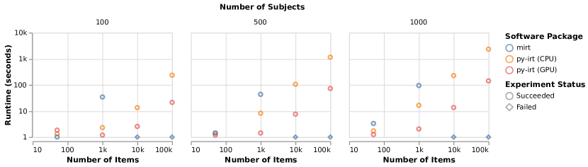
Figure 6: Runtime comparison to fit a 1PL model with varying levels of items and subjects. Beyond 1000 items, mirt does not reliably complete training.

In the next experiment, we demonstrate that py-irt-derived parameters are also reasonable across computer vision and natural language processing data sets.

1PL models are fit for the mnist (LeCun et al. 1998) and cifar (Krizhevsky et al. 2009) computer vision data sets and the Stanford Sentiment Treebank natural language processing data set (Socher et al. 2013). The irt models are fit using response pattern data from an ensemble of machine learning models (Lalor et al. 2019). These data sets are widely used in machine learning research and see use in operations research as well (e.g., Chen and Xie 2021).

In all cases, the items in the data sets identified as easy and hard seem appropriate upon inspection (Figure 7 and Table 1). The easy and difficult items in both cases are interpretable and intuitive and show how difficulty can manifest as a rare example (e.g., the blue frog), an incorrect label (e.g., the frog labeled cat), or as a case near a decision boundary (e.g., the slightly negative review). Having detailed information on item difficulty can inform data set curation and make model predictions more interpretable (Baldock et al. 2021); knowing latent item parameters also means that machine learning model ability can be estimated for more detailed analyses of model performance.

(a)

(b)

(c)

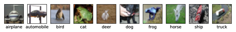
(d)

Figure 7: (Best viewed in color) The easiest (first and second rows) and hardest (third and fourth rows) items in the MNIST and CIFAR test sets. Images from (Lalor et al. 2019).

Phrase	Label	Difficulty
The stupidest, most insulting movie of 2002’s first quarter.	Negative	-2.46
An endlessly fascinating, landmark movie that is as bold as anything the cinema has seen in years.	Positive	-2.27
Still, it gets the job done - a sleepy afternoon rental.	Negative	1.78
Perhaps no picture ever made has more literally showed that the road to hell is paved with good intentions.	Positive	2.05

Table 1: Easiest and hardest items from a sentiment classification task as estimated by a 1PL model.

5 Conclusion

In this work, we introduced py-irt, a Python package for Bayesian Item Response Theory modeling. py-irt can be used to easily and efficiently fit irt models, ideal point models, and other latent trait models. The scalability of py-irt—owing to its roots in gpu-accelerated PyTorch and Pyro—allows for investigation of larger datasets like those used in machine learning evaluations. The package is available online and set up for code contributions as well. Future development for the package includes implementing amortized latent trait models and adding graded response models that can be used for Likert-scale type responses.

The code for py-irt is freely available at http://www.github.com/nd-ball/py-irt under the mit license. The Github page includes examples, an issue-tracker, and instructions for community members to contribute. Continuous integration testing ensures that new code is automatically tested before being merged into the codebase. Documentation is available at https://readthedocs.org/projects/py-irt/. The package is also available for download via the Python Package Index (PyPI): https://pypi.org/project/py-irt/.

References

- Abadi et al. (2016) Abadi M, Agarwal A, Barham P, Brevdo E, Chen Z, Citro C, Corrado GS, Davis A, Dean J, Devin M, et al. (2016) Tensorflow: Large-scale machine learning on heterogeneous distributed systems. arXiv preprint arXiv:1603.04467 .
- Baker (2001) Baker FB (2001) The Basics of Item Response Theory (ERIC), ISBN ISBN-1-886047-03-0.
- Baker and Kim (2004) Baker FB, Kim SH (2004) Item Response Theory: Parameter Estimation Techniques, Second Edition (CRC Press), ISBN 978-0-8247-5825-7.
- Baldock et al. (2021) Baldock R, Maennel H, Neyshabur B (2021) Deep learning through the lens of example difficulty. Advances in Neural Information Processing Systems 34.
- Battauz (2015) Battauz M (2015) equateIRT: An r package for IRT test equating. Journal of Statistical Software 68(1):1–22.
- Bingham et al. (2019) Bingham E, Chen JP, Jankowiak M, Obermeyer F, Pradhan N, Karaletsos T, Singh R, Szerlip P, Horsfall P, Goodman ND (2019) Pyro: Deep universal probabilistic programming. The Journal of Machine Learning Research 20(1):973–978.
- Bock and Aitkin (1981) Bock RD, Aitkin M (1981) Marginal maximum likelihood estimation of item parameters: Application of an EM algorithm. Psychometrika 46(4):443–459.
- Carlson and von Davier (2013) Carlson JE, von Davier M (2013) Item Response Theory. ETS Research Report Series 2013(2):i–69, ISSN 2330-8516, URL http://dx.doi.org/10.1002/j.2333-8504.2013.tb02335.x.
- Carpenter et al. (2017) Carpenter B, Gelman A, Hoffman MD, Lee D, Goodrich B, Betancourt M, Brubaker M, Guo J, Li P, Riddell A (2017) Stan: A probabilistic programming language. Journal of statistical software 76(1):1–32.
- Chalmers et al. (2015) Chalmers P, Pritikin J, Robitzsch A, Zoltak M (2015) Mirt: Multidimensional Item Response Theory.
- Chen and Xie (2021) Chen S, Xie W (2021) On Cluster-Aware Supervised Learning: Frameworks, Convergent Algorithms, and Applications. INFORMS Journal on Computing ISSN 1091-9856, URL http://dx.doi.org/10.1287/ijoc.2020.1053.
- Cui et al. (2017) Cui J, Rosoff H, John RS (2017) A Polytomous Item Response Theory Model for Measuring Near-Miss Appraisal as a Psychological Trait. Decision Analysis 14(2):75–86, ISSN 1545-8490, 1545-8504, URL http://dx.doi.org/10.1287/deca.2017.0345.
- de Jong et al. (2012) de Jong MG, Lehmann DR, Netzer O (2012) State-Dependence Effects in Surveys. Marketing Science 31(5):838–854, ISSN 0732-2399, 1526-548X, URL http://dx.doi.org/10.1287/mksc.1120.0722.
- de Jong et al. (2009) de Jong MG, Steenkamp JBEM, Veldkamp BP (2009) A Model for the Construction of Country-Specific Yet Internationally Comparable Short-Form Marketing Scales. Marketing Science 28(4):674–689, ISSN 0732-2399, 1526-548X, URL http://dx.doi.org/10.1287/mksc.1080.0439.
- Edgeworth (1888) Edgeworth FY (1888) The statistics of examinations. Journal of the Royal Statistical Society 51(3):599–635, ISSN 0952-8385, URL http://www.jstor.org/stable/2339898.
- Gardner et al. (2018) Gardner M, Grus J, Neumann M, Tafjord O, Dasigi P, Liu NF, Peters M, Schmitz M, Zettlemoyer LS (2018) Allennlp: A deep semantic natural language processing platform.
- Gerrish and Blei (2011) Gerrish SM, Blei DM (2011) Predicting legislative roll calls from text. Proceedings of the 28th International Conference on Machine Learning, ICML 2011.
- Hoffman et al. (2014) Hoffman MD, Gelman A, et al. (2014) The no-u-turn sampler: Adaptively setting path lengths in hamiltonian monte carlo. Journal of Machine Learning Research 15(1):1593–1623.
- Jordan et al. (1998) Jordan MI, Ghahramani Z, Jaakkola TS, Saul LK (1998) An Introduction to Variational Methods for Graphical Models. Jordan MI, ed., Learning in Graphical Models, 105–161, NATO ASI Series (Dordrecht: Springer Netherlands), ISBN 978-94-011-5014-9, URL http://dx.doi.org/10.1007/978-94-011-5014-9_5.
- Kim and Bolt (2007) Kim J, Bolt D (2007) Estimating item response theory models using markov chain monte carlo methods. Educational Measurement: Issues and Practice 26:38 – 51, URL http://dx.doi.org/10.1111/j.1745-3992.2007.00107.x.
- Kingma and Welling (2013) Kingma DP, Welling M (2013) Auto-Encoding Variational Bayes. arXiv:1312.6114 [cs, stat] .
- Krizhevsky et al. (2009) Krizhevsky A, et al. (2009) Learning multiple layers of features from tiny images .
- Lalor (2020) Lalor JP (2020) Learning Latent Characteristics of Data and Models using Item Response Theory. Ph.D. thesis, University of Massachusetts Amherst, URL http://dx.doi.org/10.7275/reha-je40.
- Lalor et al. (2016) Lalor JP, Wu H, Yu H (2016) Building an Evaluation Scale using Item Response Theory. Proceedings of the Conference on Empirical Methods in Natural Language Processing. Conference on Empirical Methods in Natural Language Processing, volume 2016, 648–657.
- Lalor et al. (2019) Lalor JP, Wu H, Yu H (2019) Learning Latent Parameters without Human Response Patterns: Item Response Theory with Artificial Crowds. Proceedings of the Conference on Empirical Methods in Natural Language Processing. Conference on Empirical Methods in Natural Language Processing, volume 2019 (Association for Computational Linguistics).
- Lalor and Yu (2020) Lalor JP, Yu H (2020) Dynamic Data Selection for Curriculum Learning via Ability Estimation. Findings of the Association for Computational Linguistics: EMNLP 2020, 545–555 (Online: Association for Computational Linguistics), URL http://dx.doi.org/10.18653/v1/2020.findings-emnlp.48.
- LeCun et al. (1998) LeCun Y, Cortes C, Burges CJ (1998) MNIST handwritten digit database. http://yann.lecun.com/exdb/mnist/.
- Lord et al. (1968) Lord FM, Novick MR, Birnbaum A (1968) Statistical theories of mental test scores URL https://psycnet.apa.org/fulltext/1968-35040-000.pdf.
- Martínez-Plumed et al. (2019) Martínez-Plumed F, Prudêncio RBC, Martínez-Usó A, Hernández-Orallo J (2019) Item response theory in AI: Analysing machine learning classifiers at the instance level. Artificial Intelligence 271:18–42, ISSN 0004-3702, URL http://dx.doi.org/10.1016/j.artint.2018.09.004.
- Martínez-Plumed et al. (2016) Martínez-Plumed F, Prudêncio RBC, Usó AM, Hernández-Orallo J (2016) Making Sense of Item Response Theory in Machine Learning. ECAI, volume 285 of Frontiers in Artificial Intelligence and Applications, 1140–1148 (IOS Press), URL http://dx.doi.org/10.3233/978-1-61499-672-9-1140.
- Natesan et al. (2016) Natesan P, Nandakumar R, Minka T, Rubright JD (2016) Bayesian Prior Choice in IRT Estimation Using MCMC and Variational Bayes. Frontiers in Psychology 7, ISSN 1664-1078, URL http://dx.doi.org/10.3389/fpsyg.2016.01422.
- Nguyen et al. (2015) Nguyen VA, Boyd-Graber J, Resnik P, Miler K (2015) Tea party in the house: A hierarchical ideal point topic model and its application to republican legislators in the 112th congress. Proceedings of the 53rd Annual Meeting of the Association for Computational Linguistics and the 7th International Joint Conference on Natural Language Processing (Volume 1: Long Papers), 1438–1448.
- Paszke et al. (2019) Paszke A, Gross S, Massa F, Lerer A, Bradbury J, Chanan G, Killeen T, Lin Z, Gimelshein N, Antiga L, et al. (2019) Pytorch: An imperative style, high-performance deep learning library. Advances in neural information processing systems 32:8026–8037.
- Pearl (1988) Pearl J (1988) Probabilistic Reasoning in Intelligent Systems: Networks of Plausible Inference (San Francisco, CA, USA: Morgan Kaufmann Publishers Inc.), ISBN 1558604790.
- Poole and Rosenthal (2017) Poole KT, Rosenthal H (2017) Ideology & congress: A political economic history of roll call voting (London, England: Routledge), 2 edition, ISBN 9780203789223, URL http://dx.doi.org/10.4324/9780203789223.
- Reckase (2009) Reckase MD (2009) Multidimensional item response theory models. Reckase, ed., Multidimensional Item Response Theory, 79–112 (New York, NY: Springer New York), ISBN 9780387899763, URL http://dx.doi.org/10.1007/978-0-387-89976-3\_4.
- Rizopoulos (2006) Rizopoulos D (2006) Ltm: An R Package for Latent Variable Modeling and Item Response Analysis. Journal of Statistical Software, Articles 17(5):1–25, ISSN 1548-7660, URL http://dx.doi.org/10.18637/jss.v017.i05.
- Rodriguez et al. (2021) Rodriguez P, Barrow J, Hoyle AM, Lalor JP, Jia R, Boyd-Graber J (2021) Evaluation Examples are not Equally Informative: How should that change NLP Leaderboards? Proceedings of the 59th Annual Meeting of the Association for Computational Linguistics and the 11th International Joint Conference on Natural Language Processing (Volume 1: Long Papers), 4486–4503 (Online: Association for Computational Linguistics), URL http://dx.doi.org/10.18653/v1/2021.acl-long.346.
- Roy et al. (2019) Roy A, Qureshi S, Pande K, Nair D, Gairola K, Jain P, Singh S, Sharma K, Jagadale A, Lin YY, Sharma S, Gotety R, Zhang Y, Tang J, Mehta T, Sindhanuru H, Okafor N, Das S, Gopal CN, Rudraraju SB, Kakarlapudi AV (2019) Performance Comparison of Machine Learning Platforms. INFORMS Journal on Computing 31(2):207–225, ISSN 1091-9856, URL http://dx.doi.org/10.1287/ijoc.2018.0825.
- Satopää et al. (2021) Satopää VA, Salikhov M, Tetlock PE, Mellers B (2021) Bias, Information, Noise: The BIN Model of Forecasting. Management Science mnsc.2020.3882, ISSN 0025-1909, 1526-5501, URL http://dx.doi.org/10.1287/mnsc.2020.3882.
- Sedoc and Ungar (2020) Sedoc J, Ungar L (2020) Item Response Theory for Efficient Human Evaluation of Chatbots. Proceedings of the First Workshop on Evaluation and Comparison of NLP Systems, 21–33 (Online: Association for Computational Linguistics), URL http://dx.doi.org/10.18653/v1/2020.eval4nlp-1.3.
- Socher et al. (2013) Socher R, Perelygin A, Wu J, Chuang J, Manning DC, Ng A, Potts C (2013) Recursive Deep Models for Semantic Compositionality Over a Sentiment Treebank. Proceedings of the 2013 Conference on Empirical Methods in Natural Language Processing, 1631–1642 (Seattle, Washington, USA: Association for Computational Linguistics).
- van Rijn et al. (2016) van Rijn PW, Sinharay S, Haberman SJ, Johnson MS (2016) Assessment of fit of item response theory models used in large-scale educational survey assessments. Large-scale Assessments in Education 4(1):10, ISSN 2196-0739, URL http://dx.doi.org/10.1186/s40536-016-0025-3.
- Vania et al. (2021) Vania C, Htut PM, Huang W, Mungra D, Pang RY, Phang J, Liu H, Cho K, Bowman SR (2021) Comparing test sets with item response theory. Proceedings of the Association for Computational Linguistics (Association for Computational Linguistics).
- Wu et al. (2020) Wu M, Davis R, Domingue B, Piech C, Goodman ND (2020) Variational item response theory: Fast, accurate, and expressive. 13th International Conference on Educational Data Mining.
- Zhang et al. (2021) Zhang X, Chen L, Gendreau M, Langevin A (2021) Learning-Based Branch-and-Price Algorithms for the Vehicle Routing Problem with Time Windows and Two-Dimensional Loading Constraints. INFORMS Journal on Computing ISSN 1091-9856, URL http://dx.doi.org/10.1287/ijoc.2021.1110.