Deep Temporal Interpolation of Radar-based Precipitation

Abstract

When providing the boundary conditions for hydrological flood models and estimating the associated risk, interpolating precipitation at very high temporal resolutions (e.g. 5 minutes) is essential not to miss the cause of flooding in local regions. In this paper, we study optical flow-based interpolation of globally available weather radar images from satellites. The proposed approach uses deep neural networks for the interpolation of multiple video frames, while terrain information is combined with temporarily coarse-grained precipitation radar observation as inputs for self-supervised training. An experiment with the Meteonet radar precipitation dataset for the flood risk simulation in Aude, a department in Southern France (2018), demonstrated the advantage of the proposed method over a linear interpolation baseline, with up to 20% error reduction.

Index Terms—  Climate & sustainability, physics-informed neural networks, spatio-temporal interpolation, satellite remote sensing

1 Introduction

Satellite observations which can consistently capture broad areas [1] are unique and effective means to achieve global scale rainfall measurement [2]. While ground-based rainfall observation networks using rain gauges [3] or weather radars provide dense and highly frequent observation such as every 10 minutes, ground observation data is often missing in Asia and African regions [4, 5] even though these regions suffer from many water related disasters.

Precipitation is one of the main causes of fatal natural disasters, as it causes flooding, landslides, and snow avalanches as well as damage to crops. The frequency and severity of these events is increasing with the increase in extreme weather events associated with acute climate change. Mathematical and computational models such as IFM [6] have become widely used tools to predict and mitigate risks to socioeconomic systems. However, for these predictions to be accurate, the underlying precipitation data driving the simulations have to be well resolved in space and time. Forecasting precipitation at very high resolutions in space and time, particularly with the aim of providing the boundary conditions for hydrological models and estimating the associated risk, is one of the most difficult challenges in meteorology [7].

This paper introduces a temporal precipitation interpolation method based on deep learning and demonstrates how the temporal resolution of it impacts an actual flood modeling results. Along with the recent work with deep learning for nowcasting [8] with topographic feature learning [9], our focus is on the temporal interpolation of precipitation for climate impact modeling. The task definition is illustrated as Figure 1. The results would be used to calibrate the impact modeling to be accurate in forecasting the disaster risks in the future, which is the motivation of the work but out of the scope for this paper.

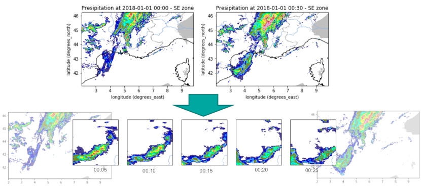
Fig. 1: An example task of temporal interpolation of precipitation. Given half-hourly snapshots from radar observation, we produce precipitation snapshots of 5 minutes.

To develop our network architecture we used SuperSloMo [10] (SSM), a multi-frame interpolation neural network, as our base network and applied the following adaptations:

• We used self-supervised learning, specific to the spatio-temporal precipitation domain, while the original paper focused on general videos of 240fps for training and 30fps for evaluation input frames.

• We used 3D vectors with an additional intensity (precipitation) transformation dimension, instead of 2D optical flow vectors.

• We added additional topographical feature integration channels, including dot products to count “rainy clouds climbing a hill”.

For unsupervised multiple video frames interpolation, we consider SSM as the state-of-the-art optical-flow approach whereas EpicFlow [11] is one of the “non-deep” state-of-the-art approaches. Deep Voxel Flow [12], an early UNet-based (thus “deep”) approach, demonstrated its advantage over EpicFlow. SSM is an advanced version of Deep Voxel Flow, demonstrating equal-or-better performance over it with additional treatment of occlusions, etc.

The rest of this paper first describes the proposed precipitation observation interpolation method along with the base one. Then, experimental results are presented, followed by some concluding remarks.

2 Temporal Precipitation Interpolation

In this paper we leverage an approach introduced by SSM [10], a high-quality variable-length multi-frame interpolation method that can interpolate a video frame at any arbitrary time step between two frames, amongst many existing works on optical flow [13, 14]. While the simple application of SuperSloMo to satellite imagery has been recently studied [15], we extend it for the purpose of precipitation interpolation and the realistic availability of supplemental data of geography.

The main idea of the original SSM work is to warp the two input images to an arbitrary time step and then adaptively fuse the warped images to generate the intermediate image, where the motion interpretation and occlusion reasoning are modeled in a single end-to-end trainable network. Specifically, they first use a flow computation Convolutional Neural Network (CNN) to estimate the bi-directional optical flow between the two input images, which is then linearly fused to approximate the required intermediate optical flow in order to warp input images. To avoid poor approximations around motion boundaries, it uses another flow interpolation CNN to refine the flow approximations and predict soft visibility maps [10].

While the experimental results in the SSM paper [10] use finer-grained training data (240fps) than prediction time (30fps), the training could have been done with the coarse-grained by considering intermediate frames in the consecutive frames or a clip as the interpolation target frames. Also, since none of the learned network parameters are time-dependent, it can produce as many intermediate frames as needed.

2.1 Base Intermediate Frame Synthesis

Given two precipitation observation inputs $I_{T}\in\mathbb{R}^{H\times W}$ at times $T=0$ and $T=1$, and an intermediate time $t\in(0,1)$, our goal is to predict the intermediate precipitation $\hat{I}_{t}\in\mathbb{R}^{H\times W}$, at time $T=t$. With multi-frames video interpolation approaches allowing arbitrary time $t\in(0,1)$ to interpolate at, such as SuperSloMo, the goal is to explicitly infer optical flows $F_{0\rightarrow t}$ and $F_{1\rightarrow t}$, which are from $I_{0}$ to $I_{t}$, and from $I_{1}$ to $I_{t}$, respectively.

The goal is then to infer an inferred intermediate frame derived from a linear combination of warped $I_{0}$ and $I_{1}$ as:

$$\hat{I}_{t}=\alpha\odot g(I_{0},F_{0\rightarrow t})+(1-\alpha)\odot g(I_{1},F_{1\rightarrow t}),$$ (1)

where $g$ is a warping function. The parameter $\alpha$ is a matrix of scalar weights $\in[0,1]$ for taking the relative importance of the reference frames into account. $\odot$ represents element-wise multiplication.

The backward warping function $g$ implemented using bilinear interpolation in SuperSloMo is defined as:

$$g^{(i)}(I,F)=\sum_{q\in\text{neighbors of}(x^{\prime(i)},y^{\prime(i)})}I^{(q)}w^{(q)},$$ (2)

where $w^{(q)}$ is a weight, generally used in bilinear interpolation, for reflecting the proximity of a reference grid $q$ from the sampling location $(x^{\prime(i)},y^{\prime(i)})$ for constructing a grid $i$. It is defined using an optical flow $F^{(i)}:=(\Delta x^{(i)},\Delta y^{(i)})$ and the target grid location $(x^{(i)},y^{(i)})$ as $(x^{\prime(i)},y^{\prime(i)})=(x^{(i)}-\Delta x^{(i)},y^{(i)}-\Delta y^{(i)})$.

2.2 Intensity Change Consistency

In applications of unsupervised deep optical flow learning, originally found in  [16], the reconstruction and photometric errors between the warped feature map from the reference image and the target image is treated as a loss to be back-propagated. If the level of intensity is not constant, then the motion estimate can be biased [13].

We introduce an additional dimension in the optical-flow vectors which represent intensity change. Instead of $F=(\Delta x,\Delta y)$, now we rely on $F=(\Delta x,\Delta y,\Delta z)$, where $\Delta z$ represents the precipitation intensity increase from original grids. The local consistency term, to be discussed in the following section, is applied to this additional dimension, as well as the original flow dimensions.

The backward warping function $g$, originally found in Equation 2, is modified as:

$$g^{(i)}(I,F)=\sum_{q\in\text{neighbors of}(x^{\prime(i)},y^{\prime(i)})}(I^{(q)}+\Delta z^{(q)})w^{(q)}.$$ (3)

2.3 Topographic Feature Integration

In addition to the precipitation observation, we utilize the topographical elevation map to predict the interpolation, as depicted in Figure 2. The entire network contains two U-Nets, which are fully convolutional neural networks. The first network takes two input images $I_{0}$ and $I_{1}$, to jointly predict the forward optical flow $F_{0\rightarrow 1}$ and backward optical flow $F_{1\rightarrow 0}$ between them. The second network then takes warped results at the target interpolation time $t$ in addition to the input images, to generate final optical flows and occlusion maps. We extend the input to the second network with topographical elevation map. In addition to feeding the map as is, we also include the feature engineered to represent the collision of rain cloud and the ground, by a dot-product of flow vector and terrain gradient.

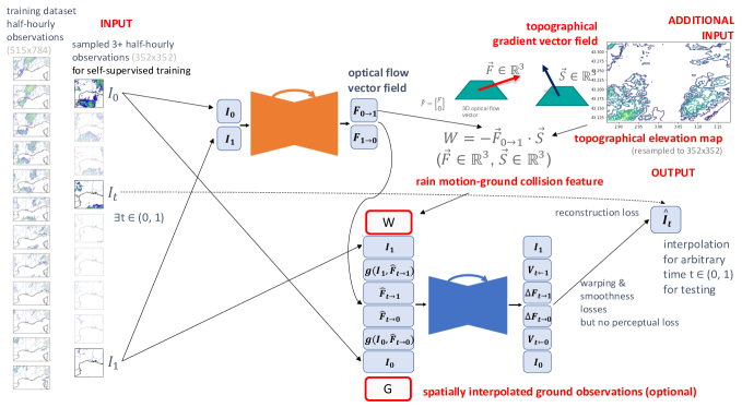
Fig. 2: The proposed architecture for temporal precipitation interpolation based on a multi-frame video interpolation method [10] and an additional geospatial feature incorporated.

2.4 Training

Instead of providing supervision for temporally fine-grained precipitation observation, which is generally difficult in practice, we train our network using the consequent observations in the original, low frequent observation of precipitation, say, consequent half-hourly observations. While SuperSloMo has been tested with supervision, the design of network itself inherently has such a capability of self-supervision.

Given input precipitation frames $I_{0}$ and $I_{1}$, an intermediate frame $I_{t}$ between them, where $t_{i}\in(0,1)$, and the prediction of intermediate frames $\hat{I}_{t}$, the loss function in SuperSloMo is a linear combination of four terms:

$$l=\lambda_{r}l_{r}+\lambda_{p}l_{p}+\lambda_{w}l_{w}+\lambda_{s}l_{s}$$ (4)

where$\lambda_{r}$, $\lambda_{p}$, $\lambda_{w}$ and $\lambda_{s}$ are weights for each loss term. They are samely set as SuperSloMo.

The reconstruction loss $l_{r}$ and the warping loss $l_{w}$ are defined in the same manner as SuperSloMo. A reconstruction loss models the distance between $I_{t}$ and $\hat{I}_{t}$, whereas a warping loss models the quality of the computed optical flow. The perceptual loss $l_{p}$, preserves details of the predictions, however it is not used in this work as we do not have a pretrained model for precipitation. For comparison, SuperSloMo used the VGG16 model for general images.

The smoothness loss $l_{s}$, is used to encourage neighboring pixels to have similar flow values as was done in SuperSloMo and is defined as :

$$l_{s}=||\Delta F_{0\rightarrow 1}||_{1}+||\Delta F_{1\rightarrow 0}||_{1}$$ (5)

but our flows $F_{0\rightarrow 1}$ and $F_{1\rightarrow 0}$ are three dimensional. The third dimension for intensity change has been introduced as described before.

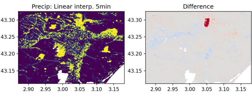
Fig. 3: Flooding simulation results using input precipitation from the linear interpolation (from 60 minutes to 5 minutes interval, left). The absolute difference from the result with the original fine temporal resolution (right) is mapped in colors (red - missing, blue - extra).

3 Experimental Results

While the interpolation was designed to work with the globally available precipitation data from IMERG, the actual experiments and demonstration were conducted based on Meteonet for validating the proposed interpolation with the ground truth precipitation observation, which is not generally available globally. Samples extracted for every 30 minutes from the interpolation target month are used for training. Every tuple of consequent 3 sampled frames in one hour (thus the middle frame as the self-supervising target) is given to a network in a random order. Otherwise we follow the experimental setting of the original SSM[10] but the training iteration was stopped at 20 epochs, where we observed general saturation of performance.

To demonstrate the impact of various precipitation interpolation methods in flood simulation with IFM, we selected an actual flooding event in the past. We select a flooding event in Aude, France back in October, 2018, which is the only flash flooding event covered by the Meteonet dataset time and area. “Several months’ worth of rain fell within a few hours overnight in Aude, leaving people stranded on rooftops”, according to a news article by Sky News. In this event, a number of areas reportedly experienced flash flooding driven by heavy rainfall in a short period. This resulted in the need for high resolution spatio-temporal rainfall information to support analysis with hydrological models to better understand what occurred on that night.

With the hypothesis that the ground topography of the area should have effects on the dynamics of the precipitation, we utilize a digital elevation model (DEM) released under the Shuttle Radar Topography Mission (SRTM) [17]. STRM is an international project aiming to generate high resolution topographic data globally. Its DEM with a one arc-second (about 30 meters) resolution is publicly available for free. We consider the elevation as a relevant variable and incorporate it as the additional input layer channels of our interpolation refinement model.

3.1 Preliminary Experiments for Impact Sensitivity

Before looking at interpolation errors, we first confirm the sensitivity of flooding impact for precipitation input errors. As a physical hydrological modeling system, we use the Integrated Flood Model (IFM), which offers fine-grained overland flood modeling with high scalability [6]. Since precipitation is an input driver for hydrological models such as IFM, the modeled results are directly affected by variations in the precipitation data.

Figure 3 shows the simulated flood extents at a single time stamp 48 hours after the start of the simulation, obtained using precipitation data from both raw 5 minutes resolution and 60-to-5 minutes linearly interpolated resolution. The difference between these two binary maps, as shown on the right, reveals the difference in flood distribution, demonstrating the sensitivity of the flood model to the precipitation input data. These results suggest that the difference of the interpolation methods applied to precipitation that drives hydrological models has potentially considerable impact to the flood simulation results, particularly in the case of flash floods that caused by local heavy rainfalls.

3.2 Interpolation Results

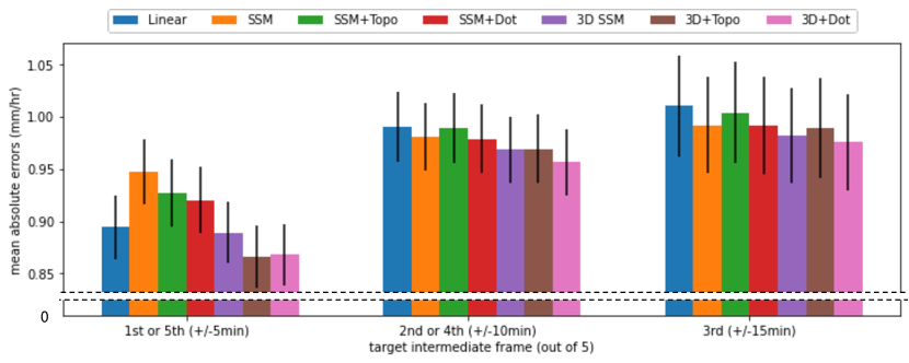
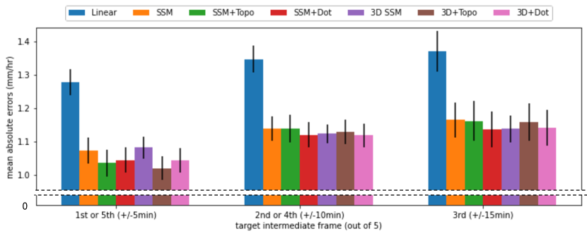
Fig. 4: Mean absolute errors (lower better) of interpolated precipitation with SEM in average of 3 days (top, including the days before/after the flooding event) and 6 hours (bottom, just before the flooding event).

Figure 4 shows the mean absolute errors from the ground truth precipitation, for each target interpolation time of 5 or 25, 10 or 20, and 15 minutes after the first reference frame. Generally the baseline liner interpolation (Linear) is good at interpolating when the target is closer to reference frames. Simply adapting SSM gives general reduction of errors. Adding our proposed adaptation of topographic features (+Topo for additional DEM input as is, +Dot for dot products of flow and gradient vectors) and intensity change consistency (3D) gives further reduction.

The advantage of the proposed approach over the baseline linear interpolation (Linear) is the largest for interpolation temporarily far from the reference input frames, and for severe weather (6 hours before the flooding event), with up-to 20% error reduction observed. The use of the intensity change (3D) generally matters for the 3-day average (including the day before and after the day of the flooding event), where weather which isn’t severe is included. Supplying dot-product (of rain cloud flow and terrain gradient, Dot) features works reasonably well.

4 Concluding Remarks

We have introduced a novel adaptation of a multi-frame video interpolation technique for temporal interpolation of precipitation observation from satellite radars. Terrain information is combined for use with temporarily coarse-grained precipitation radar observation as inputs for self-supervised training. Our experiment with the Meteonet dataset as ground-truth showed improved interpolation accuracy of our method, when compared to traditional linear interpolation.

References

- [1] G. Skofronick-Jackson, et al., “The global precipitation measurement (gpm) mission for science and society,” Bulletin of the American Meteorological Society, vol. 98, no. 8, pp. 1679 – 1695, 2017.
- [2] C. S. de Witt, et al., “Rainbench: Towards data-driven global precipitation forecasting from satellite imagery,” in Thirty-Fifth AAAI Conference on Artificial Intelligence, AAAI 2021, Thirty-Third Conference on Innovative Applications of Artificial Intelligence, IAAI 2021, The Eleventh Symposium on Educational Advances in Artificial Intelligence, EAAI 2021, Virtual Event, February 2-9, 2021. 2021, pp. 14902–14910, AAAI Press.
- [3] C. Funk, P. Peterson, M. Landsfeld, D. Pedreros, J. Verdin, S. Shukla, G. Husak, J. Rowland, L. Harrison, A. Hoell, and J. Michaelsen, “The climate hazards infrared precipitation with stations—a new environmental record for monitoring extremes,” Scientific Data, vol. 2, no. 150066, Dec 2015.
- [4] L. Bai, C. Shi, L. Li, Y. Yang, and J. Wu, “Accuracy of chirps satellite-rainfall products over mainland china,” Remote Sensing, vol. 10, no. 3, 2018.
- [5] T. Dinku, C. Funk, P. Peterson, R. Maidment, T. Tadesse, H. Gadain, and P. Ceccato, “Validation of the chirps satellite rainfall estimates over eastern africa,” Quarterly Journal of the Royal Meteorological Society, vol. 144, no. S1, pp. 292–312, 2018.
- [6] S. Singhal, S. Aneja, F. Liu, L. V. Real, and T. George, “IFM: A scalable high resolution flood modeling framework,” in Euro-Par 2014 Parallel Processing - 20th International Conference, Porto, Portugal, August 25-29, 2014. Proceedings, 2014, pp. 692–703.
- [7] M. Marrocu and L. Massidda, “Performance comparison between deep learning and optical flow-based techniques for nowcast precipitation from radar images,” Forecasting, vol. 2, no. 2, pp. 194–210, 2020.
- [8] R. Bechini and V. Chandrasekar, “An enhanced optical flow technique for radar nowcasting of precipitation and winds,” Journal of Atmospheric and Oceanic Technology, vol. 34, pp. 2637–2658, 2017.
- [9] J.-S. Proulx-Bourque and M. Turgeon-Pelchat, “Toward the use of deep learning for topographic feature extraction from high resolution optical satellite imagery,” in IGARSS 2018 - 2018 IEEE International Geoscience and Remote Sensing Symposium, 2018, pp. 3441–3444.
- [10] H. Jiang, et al., “Super SloMo: High quality estimation of multiple intermediate frames for video interpolation,” in 2018 IEEE Conference on Computer Vision and Pattern Recognition, CVPR 2018, Salt Lake City, UT, USA, June 18-22, 2018, 2018, pp. 9000–9008.
- [11] J. Revaud, P. Weinzaepfel, Z. Harchaoui, and C. Schmid, “Epicflow: Edge-preserving interpolation of correspondences for optical flow,” in IEEE Conference on Computer Vision and Pattern Recognition, CVPR 2015, Boston, MA, USA, June 7-12, 2015. 2015, pp. 1164–1172, IEEE Computer Society.
- [12] Z. Liu, R. A. Yeh, X. Tang, Y. Liu, and A. Agarwala, “Video frame synthesis using deep voxel flow,” in IEEE International Conference on Computer Vision, ICCV 2017, Venice, Italy, October 22-29, 2017. 2017, pp. 4473–4481, IEEE Computer Society.
- [13] Z. Tu, et al., “A survey of variational and CNN-based optical flow techniques,” Signal Process. Image Commun., vol. 72, pp. 9–24, 2019.
- [14] M. Zhai, X. Xiang, N. Lv, and X. Kong, “Optical flow and scene flow estimation: A survey,” Pattern Recognit., vol. 114, pp. 107861, 2021.
- [15] T. J. Vandal and R. R. Nemani, “Temporal interpolation of geostationary satellite imagery with optical flow,” IEEE Transactions on Neural Networks and Learning Systems, pp. 1–10, 2021.
- [16] Z. Ren, J. Yan, B. Ni, B. Liu, X. Yang, and H. Zha, “Unsupervised deep learning for optical flow estimation,” in Proceedings of the Thirty-First AAAI Conference on Artificial Intelligence, February 4-9, 2017, San Francisco, California, USA. 2017, pp. 1495–1501, AAAI Press.
- [17] J. J. van Zyl, “The shuttle radar topography mission (srtm): a breakthrough in remote sensing of topography,” Acta Astronautica, vol. 48, no. 5, pp. 559–565, 2001.