First joint observation by the underground gravitational-wave detector, KAGRA, with GEO 600

Abstract

We report the results of the first joint observation of the KAGRA detector with GEO 600. KAGRA is a cryogenic and underground gravitational-wave detector consisting of a laser interferometer with three-kilometer arms, and located in Kamioka, Gifu, Japan. GEO 600 is a British–German laser interferometer with 600 m arms, and located near Hannover, Germany. GEO 600 and KAGRA performed a joint observing run from April 7 to 20, 2020. We present the results of the joint analysis of the GEO–KAGRA data for transient gravitational-wave signals, including the coalescence of neutron-star binaries and generic unmodeled transients. We also perform dedicated searches for binary coalescence signals and generic transients associated with gamma-ray burst events observed during the joint run. No gravitational-wave events were identified. We evaluate the minimum detectable amplitude for various types of transient signals and the spacetime volume for which the network is sensitive to binary neutron-star coalescences. We also place lower limits on the distances to the gamma-ray bursts analysed based on the non-detection of an associated gravitational-wave signal for several signal models, including binary coalescences. These analyses demonstrate the feasibility and utility of KAGRA as a member of the global gravitational-wave detector network.

F31, F32, F33, F34

1 Introduction

The first direct observation of gravitational waves (GWs) GW150914 opened a new branch of astronomy. In their first three observing runs, Advanced LIGO and Advanced Virgo have identified 90 candidates with probability of astrophysical origin greater than 50% LIGOScientific:2018mvr ; LIGOScientific:2020ibl ; LIGOScientific:2021usb ; LIGOScientific:2021djp , all of which were consistent with being produced by the inspiral and merger of compact-object binaries comprised of BHs or NSs. During the most recent observing run, signals were detected at a rate of greater than 1 event per week LIGOScientific:2020ibl ; LIGOScientific:2021djp , and this rate is expected to grow rapidly as detector sensitivity improves KAGRA:2013pob . There is also the potential to detect GWs from other sources, such as core-collapse supernovae 2017hsn..book.1671K ; Ott_2009 cosmic strings Vachaspati:1984gt ; Sakellariadou:1990ne , and long gamma-ray bursts (GRBs) Fryer:2001zw ; vanPutten:2003hd ; Piro:2006ja ; Corsi:2009jt , which would provide probes into the astrophysics of these objects Sathyaprakash:2009xs ; LIGOScientific:2021psn and further insights into fundamental physics Sathyaprakash:2009xs ; LIGOScientific:2020tif ; LIGOScientific:2021sio .

Optimal use of GW data relies on observations by a network of detectors. Laser interferometer GW detectors are essentially all-sky monitors but have low sky-localization accuracy for short-duration transients. Determining the source position or host galaxy for short transients relies mostly on triangulation between widely separated detectors Fairhurst:2009tc ; Fairhurst:2010is ; Wen:2010cr ; Fairhurst:2017mvj ; KAGRA:2013pob ; Pankow:2019oxl . Multiple detectors with different orientations are also required to disentangle the two wave polarizations, which in turn is required, for example, for some tests of general relativity LIGOScientific:2017ycc ; GW150914 ; LIGOScientific:2018dkp ; LIGOScientific:2019fpa ; LIGOScientific:2020tif . Measuring both polarizations is also required for determining the source orientation, which is needed to determine the distance to binary sources (vital for measurements of the Hubble constant LIGOScientific:2017adf ; DES:2019ccw ; LIGOScientific:2019zcs ; LIGOScientific:2021bbr ). It can also give information on GRB beaming LIGOScientific:2017zic . Multiple detectors also provide redundancy against detector downtime and improve the sky coverage of the network.

In this paper we report the results of the first joint observation of a new detector in the global network: KAGRA. The KAGRA detector KAGRA:2020tym took scientific data from April 7 through April 20, 2020, at the end of the third observing run (O3) of the LIGO–Virgo–GEO network. The LIGO and Virgo detectors were forced to terminate operations prematurely due to the COVID-19 pandemic, but the GEO 600 (abbreviated in this paper as GEO) detector continued operations and collected data jointly with KAGRA over this period. We present the results of analyses of this joint GEO–KAGRA run data for transient GW signals. We perform four of the searches that are standard for LIGO–Virgo observing runs. Two of these scan all of the data for signals arriving from any direction at any time: a search for binary NS (BNS) coalescences TheLIGOScientific:2017qsa ; LIGOScientific:2018mvr ; LIGOScientific:2020aai ; LIGOScientific:2020ibl , and a search for generic unmodeled short transients (bursts) LIGOScientific:2016kum ; LIGOScientific:2019ppi ; LIGOScientific:2021hoh . The other two analyses are dedicated searches for binary coalescence signals and GW bursts associated with GRB events observed during the joint run LIGOScientific:2016akj ; LIGOScientific:2019obb ; LIGOScientific:2020lst ; LIGOScientific:2021iyk . No significant candidate GW events are identified, which is expected given the sensitivity of KAGRA at this early stage in its commissioning. However, the sensitivity of KAGRA is expected to improve by more than two orders of magnitude over the coming years as its design sensitivity is achieved KAGRA:2013pob . These analyses demonstrate the value KAGRA will have as a member of the global network as its sensitivity increases.

This paper is structured as follows. In Section 2 we describe the KAGRA and GEO detectors, and the joint observing run. In Section 3 we present the all-sky search for BNS coalescences. In Section 4 we present the all-sky search for generic bursts. In Section 5 we present the compact binary coalescence (CBC) and burst searches following up GRBs observed during the joint run. We conclude with a discussion of the prospects for future joint observations in Section 6.

2 GEO–KAGRA Observing Run

2.1 KAGRA

KAGRA Somiya:2011np ; Aso:2013eba ; KAGRA:2020tym is a laser interferometer GW detector with 3 km arms, located in Kamioka, Gifu, Japan. KAGRA is built underground, and uses cryogenic mirrors for four test masses in two arms. Those features help to reduce seismic and thermal noise. KAGRA uses sapphire test masses whose diameter, thickness and mass are 22 cm, 15 cm and 22.8 kg, respectively.

The construction of KAGRA started in 2010. However, the start of tunnel excavation was delayed until 2012 due to a major earthquake on March 11, 2011. The tunnel excavation was completed by May 2014, then the installation of the laser interferometer started KAGRA2018 ; KAGRA:2020tym . The initial test of KAGRA with room temperature mirrors was completed by March 2016, and the first operation of the 3 km Michelson interferometer was done from March to April 2016 KAGRA2018 ; KAGRA:2020tym . After the cryogenic systems and mirrors were installed, a test operation of the interferometer with one cryogenic mirror was performed from April 28 to May 6, 2018 KAGRA:2019htd .

By April 2019, most of the interferometer components had been installed, and the commissioning work started. In August 2019, the first lock of the Fabry–Perot Michelson interferometer configuration was achieved. The first lock of the power-recycled Fabry–Perot Michelson interferometer (PRFPMI) configuration was accomplished in January 2020. The signal readout scheme was upgraded from a conventional radio-frequency (RF) readout to a direct-current (DC) readout with an output mode cleaner in February 2020. The injected laser power was 5 W. The power recycling gain for the carrier field in the PRFPMI configuration was measured to be around 11–12. The circulating power in the Fabry–Perot arm cavities was 21–25 kW per arm.

Over the course of six months from August 2019, the detector noise floor was reduced by 3–4 orders of magnitude. A standard measure of interferometer sensitivity is the volume- and angle-averaged distance to which the inspiral of a 1.4 $M_{\odot}$–1.4 $M_{\odot}$ binary system can be detected with a matched-filter signal-to-noise ratio (SNR) of at least 8 Finn:1992xs ; KAGRA:2013pob . From February 25 to March 10, 2020, KAGRA conducted observations with a BNS observable range of about 600 kpc. After further commissioning work, the sensitivity of KAGRA was improved to reach a BNS observable range of approximately 1 Mpc by the end of March. KAGRA then performed an observation run jointly with GEO from April 7 through 20, 2020. Since the thermal noise was not a major noise source at this point, the test-mass mirrors were not cooled during this run. Further details of the detector design and construction history are given in KAGRA:2020tym .

The sensitivity of KAGRA during the joint GEO–KAGRA run was limited at low frequencies (below 100 Hz) by the local control noise of the mirror suspensions, arising from insufficiently optimised damping control filters. Above 400 Hz, the sensitivity was limited by laser shot noise. At intermediate frequencies the noise is not well-modelled but shows some coherence with environmental acoustic noise, which may arise from scattered light coupling.

During the joint run, data is flagged as being in observing mode when the PRFPMI configuration is locked with DC readout. Fixed-frequency lines are added to the test-mass feedback control signals to calibrate the data. The feedback control signals are monitored for saturations or other anomalies, and the data acquisition system is checked offline for errors. If any anomalies are found in these checks, the observing mode flag is removed. The GW searches presented in this paper are performed exclusively on data that are flagged as observing mode, except for the analysis of GRB 200415A in Section 5. At the time of GRB 200415A, the detector was locked, but there were a few personnel still near the detector following earlier maintenance work. Thus, the data at this time was not flagged as observing mode. However, subsequent investigation of the data found no anomalies, and we conclude that we can use the data around the time of GRB 200415A for GW searches.

2.2 GEO 600

GEO Luck:2010rt ; Affeldt2014Advanced600 ; Dooley2016GEOChallenges is a British–German interferometric GW detector with 600 m arms located near Hannover, Germany. Similar to other GW detectors, the design is based on a Michelson interferometer with a number of features to enhance the sensitivity. The GW signal is read out by controlling the differential arm length slightly off of the dark fringe in order to couple the differential arm motion to the direct-current power at the output. At high frequencies, the detector is limited by quantum shot noise. The shot noise originates as vacuum fluctuations entering the interferometer at the output. By replacing the normal vacuum fluctations with a squeezed vacuum, the quantum noise is reduced in the measurement quadrature PhysRevLett.126.041102 .

In contrast to the KAGRA detector, the test masses of GEO are made of fused silica and operate at room temperature Winkler2007TheOptics . Their diameter, thickness and mass are 18 cm, 10 cm and 5.6 kg, respectively. The power injected is about 3 W, which leads to about 3 kW of circulating power in the power recycling cavity which is then 1.5 kW circulating power per arm. GEO uses folding in the arms to give an optical length of 1200 m for each arm Affeldt2014Advanced600 ; Dooley2016GEOChallenges .

Normally, the GEO detector is operated in data-taking astrowatch mode when the detector is not being used for instrument science research. For the joint GEO–KAGRA run period, the detector was operated in a stable configuration that included squeezed vacuum injection for increased sensitivity. The squeezer has a high duty cycle; squeezing was applied for 97.9% of the observation time.

2.3 Joint Observing Run and Data Quality

The GEO–KAGRA joint run period was between April 7 2020 08:00 UTC and April 21 2020 00:00 UTC. Figure 1 shows representative sensitivities of the detectors during the run, as measured by the amplitude spectral density of the calibrated strain output, and the evolution of the detectors’ sensitivity over time, as measured by the BNS inspiral range.

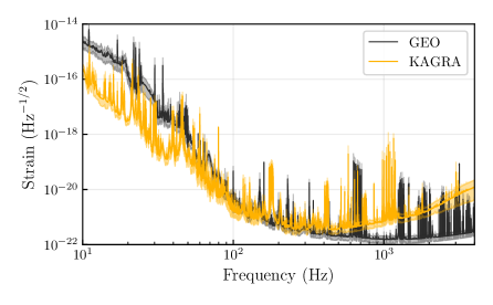
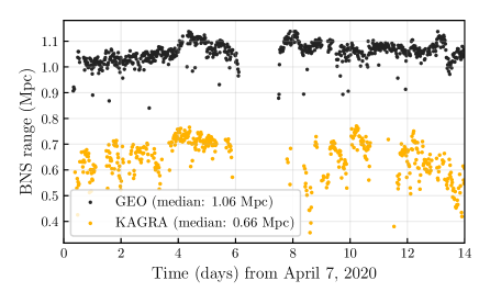
Figure 1: Left: Noise amplitude spectral density of GEO (black) and KAGRA (yellow) during the joint observing run. The solid curves show the mean sensitivity for each frequency bin and the shaded regions show the 5th and 95th percentile over the period. Narrow peaks in the spectra are due to such sources as resonances of the suspension system (violin modes) and harmonics of the electrical grid frequency (50 Hz for GEO and 60 Hz for KAGRA) openDataG ; openDataK . Right: BNS inspiral ranges for GEO and KAGRA over the joint run. The gap around day 6 and 7 was caused when both detectors were affected by bad weather and were unable to lock.

Table 1 shows the observing times and the duty cycles for two interferometers, the latter defined as the percentage of the total run duration in which the instruments were observing. The duty cycle of KAGRA was lower than that of GEO for several reasons. One was that alignment sensing and control using wavefront sensors was not implemented by the time of the run, so that the interferometer could not be operated for long periods. Furthermore, following loss of lock of the interferometer it often took a long time to adjust the alignment in order to recover lock.

	Observing time (days)	Duty cycle
GEO	10.90	79.8%
KAGRA	7.29	53.3%
coincident	6.39	46.8%

Table 1: The time length of the observing mode and the duty cycle for GEO and KAGRA for the period April 7 2020 08:00 UTC to April 21 2020 00:00 UTC.

While the quiet underground environment of KAGRA provides advantages in the operation of the instrument, KAGRA is not completely free from the effects of bad weather. The nearest coastline is approximately 40 km away. Ocean waves crashing on the shoreline constantly excite ground vibrations around $\sim$0.2 Hz, which become about one order of magnitude stronger during storms. The gap between day 6 and 7 in the BNS range time series data shown in Fig. 1 is a period when KAGRA could not operate due to a storm caused by a low-pressure system that passed through Japan at that time.

Following the joint run the vibration isolation control system has been improved and additional environmental monitors and the wavefront sensor system have been installed. This has led to an increase in KAGRA’s duty cycle.

The strain data from each interferometer is generated by processing and combining raw electronic signals coming from the differential arm length control using a detailed model of the control system including the optical response of the interferometer. Any errors in the measurements which inform the model will lead to a systematic error in the calibration. In general, systematic error is complex-valued, frequency-dependent, and time-dependent. The calibration uncertainty of the data used in this paper are within $\pm 10$% in amplitude and within $\pm 10$ $\deg$ in phase (68% C.L.) between 30 Hz and 1500 Hz and between 40 Hz and 6 kHz for KAGRA and GEO, respectively. In addition, a cleaning process PhysRevD.101.102006 using auxiliary channels is applied to the GEO data to remove some bilinear noise from the gravitational wave strain data.

We have observed many short, transient noise fluctuations, known as glitches, in each detector. During the joint observing period, the median rates of glitch triggers generated by the data-monitoring program Omicron Robinet:2015 ; Robinet:2020lbf with SNR larger than 6.5 were 10.3 per minute for GEO and 6.8 per minute for KAGRA. These values are significantly larger than the glitch rates during the first and the second parts of O3 (O3a and O3b) of LIGO–Virgo, which were 0.29–0.32 per minute, 1.1–1.2 per minute and 0.47–1.1 per minute for LIGO–Hanford, LIGO–Livingston and Virgo, respectively LIGOScientific:2020ibl ; LIGOScientific:2021djp . On the other hand, the glitch rates of GEO and KAGRA were comparable with the rate of 14 per minute in Virgo during the second observing run (O2) LIGOScientific:2020ibl , which was the first observing period for the Advanced Virgo project. The investigation of sources of glitches in GEO and KAGRA is ongoing by identifying statistical coincidences and physical couplings between the auxiliary channels and the strain channel.

One method to reduce the impact of glitches on GW searches is through the use of data-quality flags, lists of time segments that identify the status of detectors or the likely presence of a particular instrumental artefact. Three categories of data-quality flags are used in GW searches LIGOScientific:2016gtq ; LIGO:2021ppb . Category 1 flags indicate that the data have been severely impacted by noise and should not be used for astrophysical searches. Category 2 flags indicate that the data are predicted to contain non-Gaussian artefacts based on glitches in auxiliary channels and known physical couplings to the strain data. Category 3 flags indicate that the data are predicted to contain non-Gaussian artefacts based on glitches in auxiliary channels and statistically significant correlations between glitches in auxiliary channels and glitches in the strain data. GEO has introduced data-quality flags corresponding to Category 1 and Category 3. KAGRA had not introduced data-quality flags by the time of the joint run; they are planned to be introduced before the next observing run.

3 All-sky binary search

To search for compact binary coalescence (CBC) signals, we first perform a matched-filter search and then rank candidate events with a multi-dimensional classifier using the GstLAL library Messick:2016aqy ; Sachdev:2019vvd ; Hanna:2019ezx . Because of their short duration, high-mass binary coalescences are difficult to distinguish from glitches. In this search, it was found that the brief observation period did not provide a sufficiently large data set to train the ranking statistic, leading to noise features being incorrectly assigned high statistical significance. In contrast, because of their longer duration, BNS waveforms are easier to distinguish from noise transients, and despite the short observation period there is sufficient data to train the GstLAL detection system to perform well for this class of GW source. For this reason we restrict the search to BNS sources only.

Except for restricting the mass parameter range to BNS sources, the GstLAL configuration for this search is the same as those for our most recent GW transient catalogs, GWTC-2.1 LIGOScientific:2021usb and GWTC-3 LIGOScientific:2021djp , and for the O3a subsolar-mass binary search LIGOScientific:2021job , with one change: the event clustering based on the matched-filter SNR is disabled, and instead a data reduction step based on SNR and the signal-consistency test statistic is newly introduced. This change improves the GEO–KAGRA sensitive range by approximately $10\%$. This new finding will also help improve future LIGO–Virgo–KAGRA analyses.

Matched filtering is done by comparing the data to a set of template waveforms called a template bank Sathyaprakash:1991mt ; Dhurandhar:1992mw ; Owen:1995tm ; Owen:1998dk . We use the same template bank as was used in the first Advanced LIGO observing run (O1) LIGOScientific:2016vbw ; LIGOScientific:2016hpm but with the component masses restricted to the range 1 $M_{\odot}$ to 3 $M_{\odot}$, which conservatively covers the range expected for NSs LIGOScientific:2021djp . Templates are parametrized in terms of their chirp mass ${\cal M}$ which is related to the individual component masses $m_{1}$, $m_{2}$ by ${\cal M}=(m_{1}m_{2})^{3/5}/(m_{1}+m_{2})^{1/5}$. For templates with a chirp mass less than 1.73 $M_{\odot}$ the TaylorF2 waveform approximant Blanchet:2013haa ; Dhurandhar:1992mw ; Buonanno:2009zt is used, while for higher masses the reduced-order model of the SEOBNRv4 approximant Bohe:2016gbl is used. This subset of the O1 template bank was tested against a set of BNS signals with masses distributed uniformly across the search mass range and using noise power spectral densities typical of GEO and KAGRA during their joint run. The fitting factor PhysRevD.52.605 was above 0.9 for $>$99% of simulated signals, with the exceptions being simulations for the chirp mass larger than 2.4$M_{\odot}$. The fitting factor was above 0.97 (the threshold commonly used in LIGO–Virgo searches LIGOScientific:2021djp ) for all signals with chirp masses below 2 $M_{\odot}$, corresponding to component masses below 2.3 $M_{\odot}$ for an equal-mass binary.

GstLAL defines triggers as the maximum of SNR over 1 s windows which exceed a threshold of 4. It defines coincident triggers as triggers from each detector associated with the same template and with coalescence times within 32.5 ms of each other. This time window accounts for the maximum light-travel time (27.5 ms) between GEO and KAGRA as well as the uncertainty in the inferred coalescence time at each detector. Candidate events comprise both coincident triggers and non-coincident triggers. We define the network SNR as the root-sum-square of the SNR s for coincident triggers, and simply the SNR for non-coincident triggers. We discard candidate events that have network SNR below 7 because there are so many noise background events at those low SNRs that it is hard to distinguish true signals from noise.

GstLAL ranks candidate events based on the logarithm of the likelihood ratio $\mathcal{L}$, which is a measure of how signal-like a given event is. The likelihoods used in this analysis are constructed using the SNR, a signal-consistency test, the differences in time and phase between the triggers from different detectors when the candidate event consists of coincident triggers, the information of which set of detectors ({GEO}, {KAGRA}, or {GEO, KAGRA}) form the event, the sensitivity of the detectors to the exact template masses at the time of the event, the rate of triggers in each of the detectors at the time of the event, and the relative frequency with which signals are expected to be recovered by each template given the assumption that astrophysical sources are distributed uniformly in the logarithm of the masses.

GstLAL uses Monte Carlo techniques to estimate the distribution function $f(\ln\mathcal{L})$ for the log-likelihood ratios assigned to candidates resulting from the noise process. From $f(\ln\mathcal{L})$, the total number of candidates collected in the experiment, and the experiment’s duration we compute the mapping from a log likelihood-ratio threshold $\ln\mathcal{L}_{\mathrm{th}}$ to the false-alarm rate, $\mathrm{FAR}(\ln\mathcal{L}_{\mathrm{th}})$, which is the rate at which the noise process yields candidates at or above the given threshold.

3.1 Search results

For the GEO–KAGRA search, the total amount of data analyzed for each detector combination was 4.59 days for GEO-only, 0.90 days for KAGRA-only, and 6.21 days for two-interferometer observations, for a total of 11.70 days (0.032 years).

Figure 2 shows the event count as a function of the threshold on the inverse false alarm rate (iFAR). We see no significant deviation of the observed distribution from our noise model and conclude that no signal of interest has been detected. The most significant candidate is found as a coincident trigger in GEO and KAGRA at April 20 2020 14:03:28 UTC with an iFAR of 0.033 years.

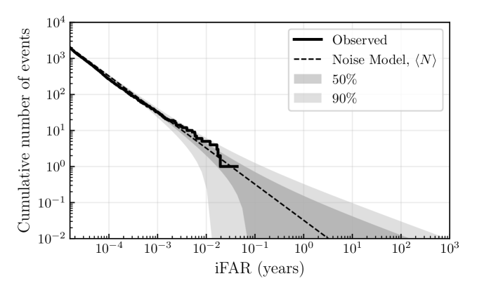
Figure 2: Event count versus threshold on iFAR. The predicted distribution due to noise is shown as the dashed line along with its 50% and 90% statistical error regions. The observed distribution is shown as the solid line.

3.2 Search sensitivity

We estimate the sensitive spacetime volume (product of sensitive volume and livetime) of this search to CBCs by adding simulated signals to the data and repeating the analysis Tiwari:2017ndi . Since GEO and KAGRA were not sensitive enough to constrain the BNS merger rate beyond the limits already set by LIGO and Virgo LIGOScientific:2021psn , we do not use an astrophysically motivated distribution for BNS masses. Instead, we measure the search sensitivity around a canonical BNS mass of $1.4\,M_{\odot}$. Specifically, the simulated signals are generated so that each component mass is normally distributed with a mean of $1.4\,M_{\odot}$ and a standard deviation of $0.01\,M_{\odot}$; i.e., according to $\mathcal{N}(1.4\,M_{\odot},[0.01\,M_{\odot}]^{2})$. The waveform approximant used for the simulated signals is TaylorT4 to 3.5 post-Newtonian order Buonanno:2002fy ; Boyle:2007ft ; Buonanno:2006ui ; Blanchet:2001ax . The signals are spaced uniformly in time with an average spacing of 10 s. Their sources are distributed uniformly in distance between 0.1 Mpc and 3 Mpc and isotropically across the sky and in orientation. Figure 3 shows the sensitive spacetime volume as a function of the iFAR threshold. This volume is computed by integrating detection efficiency over distance with appropriate weighting, where the efficiency is defined as the fraction of simulated signals that exceed the iFAR threshold within each distance bin. When we compute this fraction, we include GEO–only, KAGRA-only, and GEO–KAGRA times. The spacetime volume is a decreasing function of the threshold, approximately $3\times 10^{-2}$ Mpc³ years to $2\times 10^{-2}$ Mpc³ years for iFAR s from one per year to one per million years. Figure 3 also shows the equivalent sensitive range, defined as the radius of a sphere of the same average spatial volume, which may be compared to Figure 1. The iFAR of the most significant candidate corresponds to a range of $\sim$0.6 Mpc, which can be taken as the approximate sensitive range of this analysis.

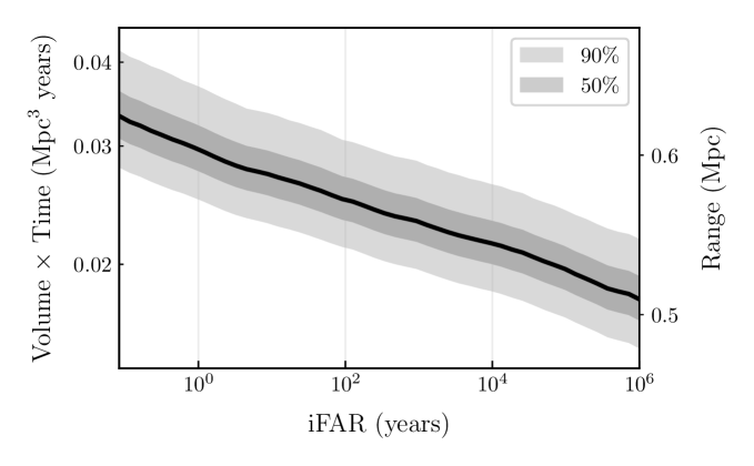
Figure 3: Sensitive spacetime volume to BNS coalescences with component masses drawn from $\mathcal{N}(1.4\,M_{\odot},[0.01\,M_{\odot}]^{2})$ as a function of the threshold on iFAR for the GstLAL binary search. The equivalent range (right axis) is also shown. The bands show the 50% and 90 % error regions, estimated as the Wilson score interval Wilson:1927 .

4 All-sky burst search

The search pipeline coherent WaveBurst (cWB) klimenko2016method ; drago2021coherent is an algorithm for the detection and reconstruction of GW transient signals with durations of typically up to a few seconds. The algorithm searches for coincident excess signal power in a network of GW detectors without assuming specific waveform models, and therefore is suitable for searching for GW transients from a range of different sources. It is used in all-sky burst searches LIGOScientific:2012cxo ; LIGOScientific:2016kum ; LIGOScientific:2019ppi , as well as for example in searches for GW s from binary coalescences LIGOScientific:2018mvr ; LIGOScientific:2020ibl ; LIGOScientific:2021djp and core-collapse supernovae LIGOScientific:2019ryq .

Analyses with cWB are performed in a wavelet domain Necula:2012zz on normalized data transformed at various resolution levels. Wavelets with amplitudes above the typical fluctuations of detector noise are selected and grouped into clusters. Clusters that are correlated in multiple detectors are identified as coherent events. For coherent events, waveforms are reconstructed based on maximum-likelihood-ratio statistics klimenko2016method . Events are ranked by their coherent network SNR $\eta_{\mathrm{c}}$ klimenko2016method and those with $\eta_{\mathrm{c}}>5$ are stored for further processing.

Due to the high rates of glitches and a large number of noise coincidences found in the GEO–KAGRA network, we apply an additional constraint in which only one polarization component of a GW candidate event is reconstructed. This constraint has been employed in other LIGO and Virgo searches LIGOScientific:2012cxo ; LIGOScientific:2016kum ; LIGOScientific:2019ppi ; LIGOScientific:2019ryq . It is effective in mitigating the background event rate, and allows the analysis to search for the GW polarization to which the network has maximum sensitivity from each sky direction Klimenko:2005xv ; Sutton:2009gi . However, for non-aligned detectors, such as GEO and KAGRA, each detector can be sensitive to different polarizations at any given sky location. In this case the constraint may lead to the rejection of real events. Also, where the network is sensitive to both polarizations, a significant portion of the signal energy contributes to the noise estimate. In extreme cases, the contribution may be so large that the signal becomes undetectable. While reconstructing both polarizations may help reduce false negative rate, lifting this constraint would increase substantially the background event rate as well as the computational cost.

To reduce further the rate of noise events falsely identified as GW signals, we apply additional selection cuts. In this work we use the network correlation coefficient $c_{\rm c}$ klimenko2016method , which is a ratio between correlated and total energy of the signal. GW signals have $c_{\rm c}\approx 1$; we exclude events with $c_{\rm c}<0.55$. We also employ the effective number of time–frequency resolution levels used for event detection and waveform reconstruction Mishra:2021tmu $n_{f}$. In total 14 resolution levels are used in this analysis. For noise events the typical values of $n_{f}$ are low; we exclude events with $n_{f}<8.9$. These thresholds are selected based on separating background events and simulated signals (described in Sections 4.1 and 4.2). We further exclude events with central frequency in the range 118–124 Hz because a significant number of background events with central frequency near 120 Hz were observed during the run. An analysis of these glitches with Omicron (Section 2) indicates they are likely associated with a single unknown noise source in KAGRA.

4.1 Background and search results

Given that the GEO–KAGRA network sensitivity is limited both at frequencies $\lesssim 100$ Hz and $\gtrsim 1$ kHz (see Figure 1), our analysis spans the frequency range of 64–1024 Hz. The data is down-sampled and periods of poor data quality are removed, similar to the all-sky searches for burst signals in O1 and O2  LIGOScientific:2016kum ; LIGOScientific:2019ppi . Intervals with at least $600$ s of continuous coincident data are required, and the total analysed coincident time between GEO and KAGRA is equal to $4.38$ days. The background event distribution is estimated by artificially time–shifting the data from one detector with respect to the other. The time shifts are multiples of 1 s, larger than the time required for a GW signal to travel between the detectors so that any identified signal is not of astrophysical origin. In total, a background livetime of $7.2$ years is obtained.

Figure 4 shows the background distribution before and after application of the $c_{\mathrm{c}}$, $n_{f}$ and central-frequency selection cuts. The post-selection-cut distribution is considered the background distribution of events for this analysis.

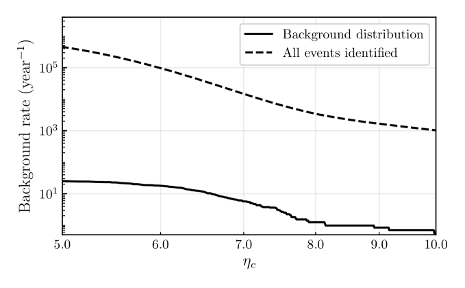
Figure 4: The rate of background events as a function of coherent network SNR $\eta_{\mathrm{c}}$ for the cWB all-sky burst search. The dashed line shows the rates for all the events. The solid line shows the rate after application of the $c_{\mathrm{c}}$, $n_{f}$ and central-frequency selection cuts.

Figure 5 shows the event count as a function of the threshold on the iFAR. Only one candidate event is identified, at April 12 2020 18:10:15 UTC with an iFAR of $0.097$ years. It is consistent with the background and is not significant enough to be considered a GW event.

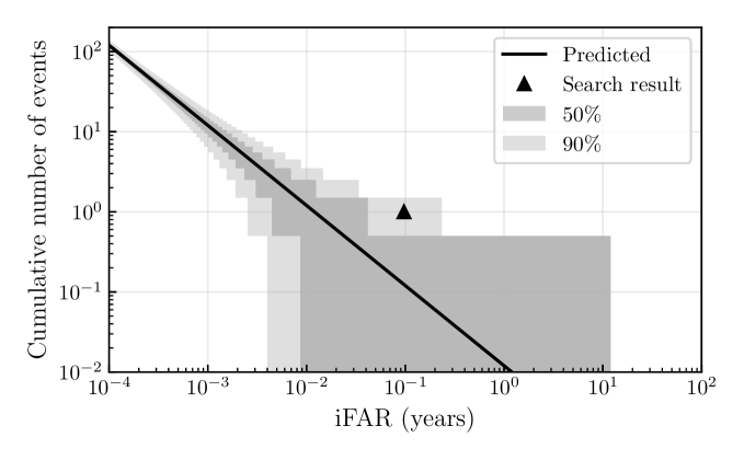
Figure 5: Cumulative number of events with central frequency in 64–1024 Hz versus iFAR found by the cWB all-sky burst search. Only a single event is identified (triangle). The shaded regions show the $50\%$ and $90\%$ Poisson uncertainties.

4.2 Search sensitivity

We estimate the search sensitivity to potential GW transients by adding simulated signals to the detector data and repeating the analysis. Similarly to other observing runs LIGOScientific:2016kum ; LIGOScientific:2019ppi ; LIGOScientific:2012cxo , we use a variety of ad hoc waveforms including sine–Gaussian wavelets (SG), Gaussian pulses (GA), and band limited white noise bursts (WNB), with frequencies and duration spanning a range of possible values. SG signals are defined by their central frequency $f_{0}$ and quality factor $Q$, which determines the duration of the signals. The GA signals are described by their duration $\tau$. The WNB signals are described by their lower frequency bound $f_{\mathrm{low}}$, bandwidth $\Delta f$, and duration $\tau$. The parameter values chosen are listed in Table 2. In addition to these ad hoc signals, two astrophysically motivated signals are used: the reconstructed signal of GW 150914 GW150914 and a simulated core-collapse supernova waveform referred to as SFHx kuroda2016new .

The simulated signals are distributed uniformly over the sky and in polarization angle. For SG waveforms, we use both elliptical and circular polarizations: the sources of circular SG s are assumed to be optimally oriented while the sources of elliptical SG s have isotropically distributed orientations. GA waveforms are linearly polarized, while WNB waveforms have uncorrelated equal-amplitude polarizations. For SFHx, we use the optimal orientation as the waveform is only available at this observing angle. Each signal is simulated at a wide range of amplitudes, characterized by the root-sum-squared strain $h_{\mathrm{rss}}$:

$$h_{\mathrm{rss}}={\bigg{\{}\int_{-\infty}^{\infty}[h_{+}^{2}(t)+h^{2}_{\times}(t)]\,\mathrm{d}t\bigg{\}}}^{1/2}.$$ (1)

These signals are then recovered using the search method described above and the detection efficiency is defined as the fraction of signals that produce an event which passes the selection cuts and has an iFAR $\geq 1$ year.

Table 2 shows for each waveform type the $h_{\mathrm{rss}}$ amplitude at which the detection efficiency reaches 50% and 90%. As mentioned earlier, the constraint employed in cWB affects the sensitivity of networks of two detectors. This effect is more prominent when the reconstructed waveform energy is distributed across different polarization components. As a result, the detection efficiencies for these waveforms are less than $90\%$ even for large values of $h_{\mathrm{rss}}$. For these waveforms, we put N/A in the column corresponding to $90\%$ detection efficiency. These $h_{\mathrm{rss}}$ limits follow the network noise spectra (Figure 1).

Morphology	50%	90%
Gaussian pulses (linear)	$h_{\mathrm{rss}}$ ($10^{-20}\,\text{Hz}^{-1/2}$)
$\tau=0.1$ ms	$5.3$	N/A
$\tau=2.5$ ms	$15.0$	N/A
sine–Gaussian wavelets (circular)
$f_{0}=100$ Hz, $Q=9$	$4.9$	$11.0$
$f_{0}=235$ Hz, $Q=9$	$1.0$	$1.9$
$f_{0}=361$ Hz, $Q=9$	$0.9$	$1.7$
sine–Gaussian wavelets (elliptical)
$f_{0}=70$ Hz, $Q=3$	$28.0$	$94.0$
$f_{0}=153$ Hz, $Q=9.0$	$4.0$	$14.0$
$f_{0}=235$ Hz, $Q=100$	$1.4$	$4.7$
$f_{0}=554$ Hz, $Q=9.0$	$1.5$	$4.3$
$f_{0}=849$ Hz, $Q=3$	$3.5$	$12.0$
White–Noise Bursts
$f_{\text{low}}$ = 150 Hz, $\Delta f=100$ Hz, $\tau=0.1$ s	$1.9$	N/A
$f_{\text{low}}$ = 300 Hz, $\Delta f=100$ Hz, $\tau=0.1$ s	$1.1$	N/A
$f_{\text{low}}$ = 700 Hz, $\Delta f=100$ Hz, $\tau=0.1$ s	$1.2$	N/A
Astrophysical Signals	distance (kpc)
GW 150914	$809$	N/A
Supernova SFHx	0.08	$0.01$

Table 2: The GW morphologies used to quantify the search sensitivity. The first column shows the waveforms used. The second and third columns show the $h_{\text{rss}}$ values at which $50\%$ and $90\%$ detection efficiencies are achieved at an iFAR of 1 year. For the astrophysical waveforms the second and third columns show the luminosity distance at which these efficiencies are achieved.

Assuming isotropic and narrow-band emission by a source, the energy emitted in GW s is given by LIGOScientific:2012cxo :

$$E_{\mathrm{GW}}=\frac{\pi^{2}c^{3}}{G}\,r^{2}f^{2}_{0}h_{\text{rss}}^{2}\,,$$ (2)

where $r$ is the distance to the source and $f_{0}$ is the central frequency. This equation is valid for unpolarized signals such as WNB s, while for SG signals, the rotating system emission has to be accounted for by multiplying the right-hand side of Eq. (2) by a factor of 2/5 Sutton:2013ooa . Using Eq. (2) and the $h_{\text{rss}}$ limits from Table 2, we can estimate the minimum energy needed to be radiated by a population of standard-candle sources at a distance of $r=10$ kpc to give a $50\%$ detection efficiency. The results are shown in Figure 6. Again, the general behavior is determined by the power spectral density of the network (Figure 1).

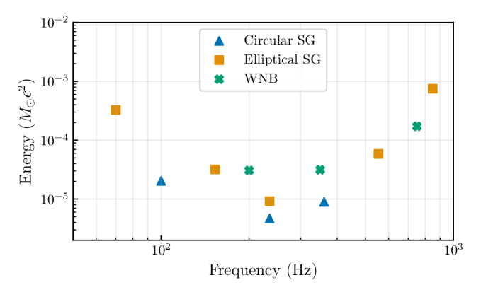
Figure 6: The GW emitted energy in units of solar masses ($M_{\odot}c^{2}$) that correspond to a $50\%$ detection efficiency with cWB at an iFAR of $\geq 1$ year, for a source located at $10$ kpc. The circular SG waveforms are indicated by triangles, the elliptical SG waveforms by squares, and the WNB waveforms by crosses.

5 Gamma-ray burst analyses

GRBs are targets of interest in GW astronomy because the astrophysical processes that power them, specifically massive stellar core collapse 2017hsn..book.1671K ; Ott_2009 ; Fryer:2001zw ; vanPutten:2003hd ; Piro:2006ja ; Corsi:2009jt and CBCs LIGOScientific:2017zic , may also emit detectable GWs. By targeting GRBs with tailored search methods we can potentially detect weaker associated GWs than would be identified with non-targeted analyses Sutton:2009gi ; Williamson:2014wma .

GRBs display a bimodality in their joint duration-spectral-hardness distribution Kouveliotou:1993yx . Long-soft GRBs (duration $\gtrsim$ 2 s) are associated with massive stellar core collapse Galama:1998ea ; Hjorth:2003jt ; Stanek:2003tw . The physics governing the bulk motion of matter during these events is complex, so we do not have robust models of the resulting GW emission, though a number of speculative models for strong GWs emission have been proposed, such as long-lived bar-mode instabilities and disk fragmentation instabilities (Fryer:2001zw, ; vanPutten:2003hd, ; Piro:2006ja, ; Corsi:2009jt, ). We therefore use a minimally modeled search algorithm X-Pipeline Sutton:2009gi ; Was:2012zq to target these GRBs.

Short-hard GRBs (duration $<$ 2 s) can be produced by NS binary coalescences, a connection that was long proposed Blinnikov:2018boq ; Eichler:1989ve ; Paczynski:1991aq ; Narayan:1992iy and observationally confirmed by the multimessenger studies of GW170817/GRB 170817A TheLIGOScientific:2017qsa ; LIGOScientific:2017zic ; GBM:2017lvd ; Lazzati:2017zsj ; Alexander:2018dcl ; Mooley:2018dlz ; Ghirlanda:2018uyx ; Fong:2019vgn . We therefore target them with a modeled CBC search algorithm PyGRB Harry:2010fr ; Williamson:2014wma in addition to the more generic minimally modeled X-Pipeline.

During the joint GEO–KAGRA run, 4 GRBs were detected coinciding with science data taking in both GEO and KAGRA; see Table 3. Our minimally modeled search algorithm was able to analyze all of these given its data requirements. GRB 200415A and GRB 200420A were short duration, therefore our modeled search algorithm was also used to analyze them. GRB 200415A was subsequently associated Roberts:2021udn ; Svinkin:2021wcp with a magnetar giant flare in the nearby galaxy NGC253 at 3.5 Mpc based on its sky position, temporal and spectral properties and inferred energy. All GRB properties were taken from the Fermi Gamma-ray Burst Monitor (GBM) Catalog fermigbmcatalog ; vonKienlin:2020xvz ; Bhat:2016odd ; vonKienlin:2014nza ; Gruber:2014iza , with one exception: the minimally modeled analysis of GRB 200415A took sky position data from a preliminary IPN triangulation gcn27595 for practical reasons. Given the coarse angular sensitivity of the GW detector network, the very small difference does not affect the results in any significant way.

GRB Name	Data Source	Type	Analysis
200412A	Fermi-GBM	Long	X-Pipeline
200415A	Fermi-GBM, IPN	Short	X-Pipeline & PyGRB
200418A	Fermi-GBM	Long	X-Pipeline
200420A	Fermi-GBM	Short	X-Pipeline & PyGRB

Table 3: GRBs observed during GEO–KAGRA run times when both detectors were taking science-quality data. GRB 200415A and GRB 200420A were short-duration GRBs, and so are analysed by both searches.

5.1 Binary coalescence search targeting short GRBs

By targeting the times and sky positions of short GRBs, we can perform a deep, coherent matched filter analysis for associated GWs from BNS and NS–BH (NSBH) binaries. This analysis is called PyGRB Harry:2010fr ; Williamson:2014wma , and forms part of the larger PyCBC analysis toolkit pycbc with key components in the LALSuite library lalsuite . This approach has been used in many previous observing runs of the LIGO and Virgo detectors LIGOScientific:2016akj ; LIGOScientific:2019obb ; LIGOScientific:2020lst ; LIGOScientific:2021iyk and here we deploy a PyGRB analysis that is functionally identical to that used in the most recent LIGO–Virgo analyses LIGOScientific:2020lst ; LIGOScientific:2021iyk , with only some changes to the configuration that are appropriate for the data being analyzed, as outlined below.

The PyGRB search performs a matched filter coherently across the operational GW detector network around the time of each short GRB. In this analysis we filter in the frequency range 40–1000 Hz with a bank of template waveforms Owen:1998dk ; Capano:2016dsf generated with an aligned-spin point-particle model, IMRPhenomD, that includes inspiral, merger, and ringdown phases Husa:2015iqa ; Khan:2015jqa . The bank includes waveforms representing BNS and NSBH systems, where NSs have dimensionless spins $\leq 0.05$. Within these bounds, NSBH templates are further constrained to the region in parameter space where the combination of masses and spins could give rise to tidal disruption of the NS, and therefore potentially produce a GRB following Foucart:2012nc ; Pannarale:2014rea , assuming a very stiff 2H equation of state Kyutoku:2010zd and requiring a non-zero remnant mass. Additionally, we place an inclination constraint motivated by the expected SGRBsurvey2012 ; Fong:2013lba ; Panaitescu:2005er ; Troja:2016vzw small inclination angles for GRB progenitors due to GRB beaming. This is imposed by filtering with only circularly polarized templates Williamson:2014wma , corresponding to binary systems with inclination angles $\theta_{JN}$ between the total angular momentum axes $\hat{J}$ and the line-of-sight $\hat{N}$ of $0\,\deg$ or $180\,\deg$. This constraint improves sensitivity to signals with small inclinations ($\lesssim 30\,\deg$ or $\gtrsim 150\,\deg$).

We tile the reported sky error region of each GRB and filter at each sky point with our constrained template bank Williamson:2014wma to obtain a coherent SNR statistic for the network. We place thresholds of 4 on single detector SNRs and 6 on the coherent network SNR. Surviving triggers are then re-weighted or cut according to signal consistency checks Allen:2005fk ; Harry:2010fr ; Williamson:2014wma , to produce the search detection statistic.

We consider a 6 s window spanning $[-5,+1)\,\mathrm{s}$ about the reported GRB Earth-crossing time as the on-source where an associated GW event may be found. This is compared to an off-source window that is used to characterize the search background, which typically contains up to $\sim 90\,\mathrm{min}$ of data surrounding the on-source time. The loudest (most significant) candidate event in the on-source, as defined by the detection statistic, is compared to a list containing the most significant background events from each of the 6 s background trials within the off-source. Additional background trials are obtained by time shifting the data streams relative to one another by amounts greater than the light travel time between the detectors Williamson:2014wma , similar to the approach described in Section 4. This comparison between on-source and background trials results in a $p$-value for the candidate on-source event.

The short GRB triggers during the analysis period with available data from both interferometers were GRB 200415A and GRB 200420A. The loudest candidates within the on-source windows had $p$-values of 0.43 and 0.45 respectively, consistent with being due to background noise.

The sensitivity of the search is evaluated through the use of simulated GW signals inserted throughout the off-source data and spread across the region(s) of the sky corresponding to the positional uncertainty of the GRB trigger. These simulated signals correspond to events drawn from three potential astrophysical populations: NSBH with aligned spins, NSBH with isotropically oriented spins, and BNS with isotropically oriented spins. We draw NS masses from normal distributions centered on 1.4 $M_{\odot}$ with standard deviations of $0.2M_{\odot}$ and $0.4M_{\odot}$ for BNS and NSBH systems respectively Ozel:2012ax ; Kiziltan:2013oja , limited within the range $[1.0,3.0]M_{\odot}$. The wider NSBH distribution reflects the greater uncertainty surrounding NSBH system properties. NS dimensionless spin magnitudes are drawn uniformly in the range $[0,0.4]$, with the upper limit corresponding to the fastest spinning pulsar observed Hessels:2006ze . BH masses are drawn from ${\cal N}(10M_{\odot},[6M_{\odot}]^{2})$ limited within the range $[3,15]M_{\odot}$ and dimensionless spin magnitudes uniformly in the range $[0,0.98]$ Miller:2014aaa . Spins are isotropically oriented except for the aligned spin NSBH population. Inclination angles $\theta_{JN}$ are drawn uniformly in $\cos\theta_{JN}$ for $\theta_{JN}\in[0,30^{\circ}]\cup[150^{\circ},180^{\circ}]$. NSBH systems are then rejected if they do not meet the same NS disruption condition as applied to the template bank Foucart:2012nc ; Pannarale:2014rea . NSBH signals are generated with a point-particle effective-one-body model for the inspiral–merger–ringdown phases that incorporates orbital precession effects and is tuned to numerical-relativity simulations, SEOBNRv3 Pan:2013rra ; Taracchini:2013rva ; Babak:2016tgq . BNS signals are generated with a time-domain approximation to 3.5 post-Newtonian order for the inspiral phase, SpinTaylorT2 Sathyaprakash:1991mt ; Blanchet:1996pi ; Mikoczi:2005dn ; Arun:2008kb ; Bohe:2013cla ; Bohe:2015ana ; Mishra:2016whh .

In the case of no compelling candidate event being identified in the on-source, these simulated signals allow for exclusion distances to be quoted. A 90% exclusion distance corresponds to the distance within which 90% of a population of simulated signals were recovered with a detection statistic at least as large as the loudest on-source candidate event; at greater distances the recovered fraction of signals drops. For GRB 200415A we report 90% exclusion distances of 0.91 Mpc for BNS systems, 1.08 Mpc for isotropically spinning NSBH, and 1.45 Mpc for aligned-spin NSBH. At a distance of 3.5 Mpc, corresponding to NGC 253, exclusion confidences for these three populations are 0%, 2%, and 9% respectively, too low to be able to confidently exclude any such binary merger as the progenitor of GRB 200415A. These exclusion curves are shown in Figure 7. For GRB 200420A we report 90% exclusion distances of 0.15 Mpc for BNS systems, 0.21 Mpc for isotropically spinning NSBH, and 0.17 Mpc for aligned-spin NSBH. The injection recovery was limited in this case by the large sky error of the GRB. The reported GBM $1\sigma$ statistical uncertainty (averaged over the error ellipse vonKienlin:2014nza ) was $27.3\,\deg$ gcn27609 , and was used to generate a two-dimensional normal distribution on the sky from which injection sky positions were drawn. This resulted in a population of injections spanning a large area on the sky within which the interferometer sensitivities varied significantly, including regions with severely reduced range. As a result, a non-negligible fraction of nearby injections were undetectable.

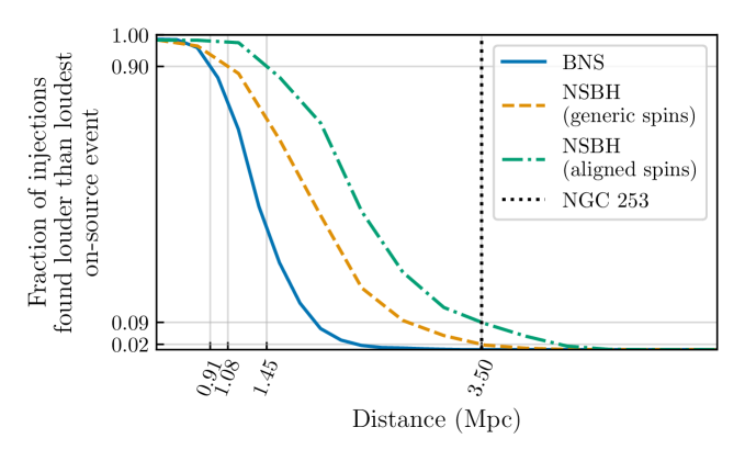
Figure 7: Exclusion distance curves for GRB 200415A. We show the curves for each of our three injection populations: BNSs (blue solid), isotropically spinning NSBHs (orange dashed), and aligned-spin NSBHs (green dot-dashed). The respective 90% confidence exclusion distances of 0.91 Mpc, 1.08 Mpc, and 1.45 Mpc are marked, as are the confidence levels corresponding to the distance to NGC 253 (3.5 Mpc; black dotted), which are 0%, 2%, and 9% respectively. Thus the search sensitivity is not sufficient to confidently exclude a binary merger in NGC 253 as the progenitor based on the available GW data.

5.2 Search for generic bursts associated with GRBs

X-Pipeline Sutton:2009gi ; Was:2012zq is an analysis package that combines data from multiple detectors coherently to detect minimally modeled GW transient signals associated with events such as GRB s, core-collapse supernovae, and fast radio bursts. It is used regularly for such searches of LIGO–Virgo data LIGOScientific:2016jvu ; LIGOScientific:2016rmm ; LIGOScientific:2019ccu ; LIGOScientific:2016akj ; LIGOScientific:2017zic ; LIGOScientific:2019obb ; LIGOScientific:2020lst .

For each GRB X-Pipeline constructs a grid of sky positions covering that GRB’s sky localisation error box. For this analysis linear grids are used, which have been shown to be a computationally efficient way to cover large error boxes for two-detector networks without significant loss of sensitivity LIGOScientific:2014zwy . For each grid point a coherent analysis is performed. The frequency range of the search is increased from the standard values of [20, 500] Hz to [30,1100] Hz to account for GEO’s better sensitivity at higher frequencies. The on-source window is [$-$600 s, $+$max(60 s,$T_{90}$)] about the GRB Earth-crossing time, where $T_{90}$ is the reported GRB duration. This window is large enough to account for any reasonable time delay between the GW and gamma-ray emission koshut1995gamma ; aloy2000relativistic ; macfadyen2001supernovae ; zhang2003relativistic ; lazzati2005precursor ; wang2007grb ; burlon2008precursors ; burlon2009time ; lazzati2009very ; vedrenne2009gamma . An exception to this window choice is made for GRB 200415A, for which KAGRA was not operating in a stable locked state until less than 600 s before the GRB event. For this GRB we use an on-source window of [$-$519, $+$60] s. The off-source window consists of all data within $\pm$90 min of the GRB, including time shifts similar to those used by cWB. The total amount of off-source data analysed is between $5\times 10^{3}$ and $3\times 10^{4}$ times the on-source duration for each GRB, allowing $p$-values of order $10^{-4}$ to be measured. Finally, simulated signals are added to the on-source window; these are used both for estimating the sensitivity of the search and for automated tuning of X-Pipeline’s background rejection tests.

The same procedure is used for the on-source, off-source, and simulation analyses. The data are whitened, then Fourier transformed with transform durations of [1/256, 1/128, …, 2] s. The Fourier-transformed data are combined to form time–frequency maps for each detector. From these maps the highest 1% of pixels are grouped into clusters. For each cluster the data from the different detectors is combined in multiple combinations to estimate the signal energy consistent with different GW polarizations and to give various measures of correlation between detectors. When clusters from different sky positions or Fourier transform durations overlap in time-frequency, the most significant is retained. The clusters are then checked for coherency between detectors to reduce the background. The thresholds for these background rejection tests are selected to maximise the detection efficiency at a user-specified false-alarm probability ($10^{-4}$ for this analysis), using a subset of the off-source and simulation clusters. The optimised thresholds are then applied to the on-source clusters and to the remaining off-source and simulation clusters. The surviving on-source clusters are our candidate events. Each is assigned a $p$-value by comparing to the distribution of surviving off-source events. The sensitivity as a function of signal amplitude or source distance is evaluated as the fraction of simulated signals that give surviving events with $p$-values lower than the lowest $p$-value of the on-source events.

Of the four GRBs analysed, the lowest $p$-value for any on-source event was $p=$ 0.132 for GRB 200412A. This is consistent with the null hypothesis given the number of GRBs analysed. We therefore conclude there is no evidence for GW emission associated with any of the four GRBs analysed. Figure 8 shows the 90% confidence level lower limit on the distance for each of the GRBs for several emission models: the accretion-disk instability model A of vanPutten:2001sw ; vanPutten:2014kja ; and circularly polarized sine–Gaussian LIGOScientific:2016akj signals with central frequencies of 150 Hz, 500 Hz, and 1000 Hz where we assume an energy emission of $10^{-2}\,M_{\odot}c^{2}$ ($1.8\times 10^{52}\,\mathrm{erg}$) in GWs. We see that in each case our exclusion distances are of order 100 kpc (the analyses of GRB 200412A and GRB 200420A did not produce 90% exclusion distances for the 1000 Hz sine–Gaussians above 10 kpc). This is not enough to test the magnetar giant flare hypothesis for GRB 200415A Svinkin:2021wcp .

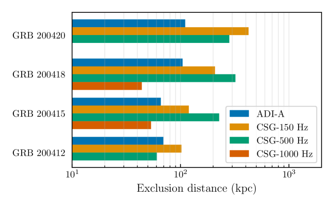
Figure 8: The 90% confidence-level exclusion distances for each of the GRBs analysed by the X-Pipeline generic burst search, for the accretion disk instability (ADI) signal model A and for circular sine–Gaussian (CSG) signals at 150 Hz, 500 Hz, and 1000 Hz. For a given GRB and signal model this is the distance within which 90% of simulated signals inserted into off-source data are recovered passing all background rejection tests and with a significance greater than the loudest on-source candidate event (if any).

6 Summary and Discussion

We have presented the results of the first joint observation of the KAGRA detector with GEO, performed during April 7–20 2020. The coincident observational data from GEO and KAGRA were analysed jointly to look for transient GW signals, including neutron-star binary coalescences and generic unmodeled transients. We also performed dedicated searches for CBC signals and generic transients associated with GRBs observed during the joint run. No candidate GW events were identified.

In the all-sky BNS search, the most significant candidate from the analysis of 0.032 years of data has an iFAR of 0.033 years, consistent with background. The sensitive spacetime volume to BNS coalescences was estimated as a function of iFAR, and we found that the iFAR of the most significant event corresponds to a sensitive distance of $\sim$0.6 Mpc, comparable to that expected from the noise spectra.

In the all-sky burst search, the most significant candidate from the analysis of 0.012 years of data has an iFAR of $0.097$ years which is not significant enough to be considered a likely GW event. The sensitivity of the search was estimated in terms of the minimal detectable root-sum-square signal amplitude and minimum detectable signal energy at a fixed distance. We find minimal detectable energies of around $10^{-6}\,M_{\odot}c^{2}$ to $10^{-3}\,M_{\odot}c^{2}$ for sources at 10 kpc. These sensitivities are consistent with the amplitude spectral densities of the detectors.

The searches for CBCs and generic transient signals associated with GRBs found no candidate events, with the lowest $p$-value for any GRB being 0.132. For GRB 200415A, the dedicated CBC search set a 90% exclusion distance of 0.91 Mpc for BNS systems, 1.08 Mpc for generically spinning NSBH, and 1.45 Mpc for aligned-spin NSBH. At a distance of 3.5 Mpc, corresponding to NGC 253, the exclusion confidences for these populations are 0%, 2% and 9% respectively. The sensitivity of the generic burst search was evaluated for several GW emission models, giving 90% exclusion distances of order 100 kpc for sources emitting $10^{-2}\,M_{\odot}c^{2}$ energy in GWs. These results are not strong enough to test the binary merger or magnetar hypotheses for the progenitor of GRB 200415A.

The lack of detected GWs in this run is expected given the sensitivity of the GEO–KAGRA network at the time. However, the sensitivity of KAGRA is expected to improve by more than two orders of magnitude later in this decade KAGRA:2013pob , becoming comparable to that of the LIGO and Virgo detectors. Our analyses have demonstrated the ability to incorporate KAGRA data into standard transient search pipelines that have been used to detect GWs in LIGO and Virgo data. Adding KAGRA to the LIGO–Virgo network will improve the sky-localization accuracy and increase the number of events detected with 3 or more detectors simultaneously Wen:2010cr ; Schutz:2011tw . KAGRA is planning to join the forth observing run of the advanced-detector network. We look forward to KAGRA’s scientific contributions in the coming years as a member of the global GW detector network.

The full O3GK detector strain data and data products associated with this paper are available through Gravitational Wave Open Science Center O3GKDataRelease .

References

- (1) B. P. Abbott et al., Phys. Rev. Lett., 116(6), 061102 (2016), arXiv:1602.03837.
- (2) B. P. Abbott et al., Phys. Rev. X, 9(3), 031040 (2019), arXiv:1811.12907.
- (3) R. Abbott et al., Phys. Rev. X, 11, 021053 (2021), arXiv:2010.14527.
- (4) R. Abbott et al. (2021), arXiv:2108.01045.
- (5) R. Abbott et al. (2021), arXiv:2111.03606.
- (6) B. P. Abbott et al., Living Rev. Rel., 23(1), 3 (2020), arXiv:1304.0670.
- (7) K. Kotake and T. Kuroda, Gravitational Waves from Core-Collapse Supernovae, page 1671 (2017).
- (8) C. D. Ott, Class. Quant. Grav., 26(6), 063001 (2009), 0809.0695.
- (9) T. Vachaspati and A. Vilenkin, Phys. Rev. D, 31, 3052 (1985).
- (10) M. Sakellariadou, Phys. Rev. D, 42, 354–360, [Erratum: Phys. Rev. D 43,4150(1991)] (1990).
- (11) C. L. Fryer, D. E. Holz, and S. A. Hughes, Astrophys. J., 565, 430–446 (2002), astro-ph/0106113.
- (12) M. H. P. M. van Putten, A. Levinson, H. K. Lee, T. Regimbau, M. Punturo, and G. M. Harry, Phys. Rev. D, 69, 044007 (2004), gr-qc/0308016.
- (13) A. L. Piro and E. Pfahl, Astrophys. J., 658, 1173 (2007), astro-ph/0610696.
- (14) A. Corsi and P. Mészáros, Astrophys. J., 702, 1171–1178 (2009), arXiv:0907.2290.
- (15) B. S. Sathyaprakash and B. F. Schutz, Living Rev. Rel., 12, 2 (2009), arXiv:0903.0338.
- (16) R. Abbott et al. (2021), arXiv:2111.03634.
- (17) R. Abbott et al., Phys. Rev. D, 103(12), 122002 (2021), arXiv:2010.14529.
- (18) R. Abbott et al. (2021), arXiv:2112.06861.
- (19) S. Fairhurst, New J. Phys., 11, 123006, [Erratum: New J.Phys. 13, 069602 (2011)] (2009), arXiv:0908.2356.
- (20) S. Fairhurst, Class. Quant. Grav., 28, 105021 (2011), arXiv:1010.6192.
- (21) L. Wen and Y. Chen, Phys. Rev. D, 81, 082001 (2010), arXiv:1003.2504.
- (22) S. Fairhurst, Class. Quant. Grav., 35(10), 105002 (2018), arXiv:1712.04724.
- (23) C. Pankow, M. Rizzo, K. Rao, C. P. L. Berry, and V. Kalogera, Astrophys. J., 902(1), 71 (2020), arXiv:1909.12961.
- (24) B. P. Abbott et al., Phys. Rev. Lett., 119(14), 141101 (2017), arXiv:1709.09660.
- (25) B. P. Abbott et al., Phys. Rev. Lett., 123(1), 011102 (2019), arXiv:1811.00364.
- (26) B. P. Abbott et al., Phys. Rev. D, 100(10), 104036 (2019), arXiv:1903.04467.
- (27) B. P. Abbott et al., Nature, 551(7678), 85–88 (2017), arXiv:1710.05835.
- (28) M. Soares-Santos et al., Astrophys. J. Lett., 876(1), L7 (2019), arXiv:1901.01540.
- (29) B. P. Abbott et al., Astrophys. J., 909(2), 218 (2021), arXiv:1908.06060.
- (30) R. Abbott et al. (2021), arXiv:2111.03604.
- (31) B. P. Abbott et al., Astrophys. J. Lett., 848(2), L13 (2017), arXiv:1710.05834.
- (32) T. Akutsu et al., Prog. Theor. Exp. Phys., 2021(5) (2020), arXiv:2005.05574.
- (33) B. P. Abbott et al., Phys. Rev. Lett., 119(16), 161101 (2017), arXiv:1710.05832.
- (34) B. P. Abbott et al., Astrophys. J. Lett., 892(1), L3 (2020), arXiv:2001.01761.
- (35) B. P. Abbott et al., Phys. Rev. D, 95(4), 042003 (2017), arXiv:1611.02972.
- (36) B. P. Abbott et al., Phys. Rev. D, 100(2), 024017 (2019), arXiv:1905.03457.
- (37) R. Abbott et al., Phys. Rev. D, 104(12), 122004 (2021), arXiv:2107.03701.
- (38) B. P. Abbott et al., Astrophys. J., 841(2), 89 (2017), arXiv:1611.07947.
- (39) B. P. Abbott et al., Astrophys. J., 886, 75 (2019), arXiv:1907.01443.
- (40) R. Abbott et al., Astrophys. J., 915, 86 (2021), arXiv:2010.14550.
- (41) R. Abbott et al. (2021), arXiv:2111.03608.
- (42) K. Somiya, Class. Quant. Grav., 29, 124007 (2012), arXiv:1111.7185.
- (43) Y. Aso, Y. Michimura, K. Somiya, M. Ando, O. Miyakawa, T. Sekiguchi, D. Tatsumi, and H. Yamamoto, Phys. Rev. D, 88(4), 043007 (2013), arXiv:1306.6747.
- (44) T. Akutsu et al., Prog. Theor. Exp. Phys., 2018(1), 013F01 (2018), arXiv:1712.00148.
- (45) T. Akutsu et al., Class. Quant. Grav., 36(16), 165008 (2019), arXiv:1901.03569.
- (46) L. S. Finn and D. F. Chernoff, Phys. Rev. D, 47, 2198–2219 (1993), gr-qc/9301003.
- (47) H. Lück et al., J. Phys. Conf. Ser., 228, 012012 (2010), arXiv:1004.0339.
- (48) C. Affeldt, K. Danzmann, K. L. Dooley, H. Grote, M. Hewitson, S. Hild, J. Hough, J. Leong, H. Lück, M. Prijatelj, S. Rowan, A. Rüdiger, R. Schilling, .R Schnabel, E. Schreiber, B. Sorazu, K. A. Strain, H. Vahlbruch, B. Willke, W. Winkler, and H. Wittel, Class. Quant. Grav., 31(22), 224002 (2014).
- (49) K. L. Dooley, J. R. Leong, T. Adams, C. Affeldt, A. Bisht, C. Bogan, J. Degallaix, C. Gräf, S. Hild, J. Hough, A. Khalaidovski, N. Lastzka, J. Lough, H. Lück, D. Macleod, L. Nuttall, M. Prijatelj, R. Schnabel, E. Schreiber, J. Slutsky, B. Sorazu, K. A. Strain, H. Vahlbruch, M. Wa̧s, B. Willke, H. Wittel, K. Danzmann, and H. Grote, Class. Quant. Grav., 33(7), 075009 (2016), arXiv:1510.00317.
- (50) J. Lough, E. Schreiber, F. Bergamin, H. Grote, M. Mehmet, H. Vahlbruch, C. Affeldt, M. Brinkmann, A. Bisht, V. Kringel, H. Lück, N. Mukund, S. Nadji, B. Sorazu, K. Strain, M. Weinert, and K. Danzmann, Phys. Rev. Lett., 126, 041102 (2021), arXiv:2005.10292.
- (51) W. Winkler, K. Danzmann, H. Grote, M. Hewitson, S. Hild, J. Hough, H. Lück, M. Malec, A. Freise, K. Mossavi, S. Rowan, A. Rüdiger, R. Schilling, J.R. Smith, K.A. Strain, H. Ward, and B. Willke, Opt. Commun., 280(2), 492–499 (2007).
- (52) https://gw-openscience.org/O3/O3GK_GEO_speclines/ (2022).
- (53) https://gw-openscience.org/O3/O3GKspeclines/ (2022).
- (54) N. Mukund, J. Lough, C. Affeldt, F. Bergamin, A. Bisht, M. Brinkmann, V. Kringel, H. Lück, S. Nadji, M. Weinert, and K. Danzmann, Phys. Rev. D, 101, 102006 (2020), arXiv:2001.00242.
- (55) F. Robinet, Omicron: An algorithm to detect and characterize transient noise in gravitational-wave detectors, https://tds.virgo-gw.eu/ql/?c=10651 (2015).
- (56) F. Robinet, N. Arnaud, N. Leroy, A. Lundgren, D. Macleod, and J. McIver, SoftwareX, 12, 100620 (2020), arXiv:2007.11374.
- (57) B. P. Abbott et al., Class. Quant. Grav., 33(13), 134001 (2016), arXiv:1602.03844.
- (58) D. Davis et al., Class. Quant. Grav., 38(13), 135014 (2021), arXiv:2101.11673.
- (59) C. Messick et al., Phys. Rev. D, 95(4), 042001 (2017), arXiv:1604.04324.
- (60) S. Sachdev et al. (2019), arXiv:1901.08580.
- (61) C. Hanna et al., Phys. Rev. D, 101(2), 022003 (2020), arXiv:1901.02227.
- (62) R. Abbott et al. (2021), arXiv:2109.12197.
- (63) B. S. Sathyaprakash and S. V. Dhurandhar, Phys. Rev. D, 44, 3819–3834 (1991).
- (64) S. V. Dhurandhar and B. S. Sathyaprakash, Phys. Rev. D, 49, 1707–1722 (1994).
- (65) B. J. Owen, Phys. Rev. D, 53, 6749–6761 (1996), gr-qc/9511032.
- (66) B. J. Owen and B. S. Sathyaprakash, Phys. Rev. D, 60, 022002 (1999), arXiv:gr-qc/9808076.
- (67) B. P. Abbott et al., Phys. Rev. D, 93(12), 122003 (2016), arXiv:1602.03839.
- (68) B. P. Abbott et al., Astrophys. J. Lett., 832(2), L21 (2016), arXiv:1607.07456.
- (69) L. Blanchet, Living Rev. Rel., 17, 2 (2014), arXiv:1310.1528.
- (70) A. Buonanno, B. Iyer, E. Ochsner, Y. Pan, and B. S. Sathyaprakash, Phys. Rev. D, 80, 084043 (2009), arXiv:0907.0700.
- (71) A. Bohé et al., Phys. Rev. D, 95(4), 044028 (2017), arXiv:1611.03703.
- (72) T. A. Apostolatos, Phys. Rev. D, 52, 605–620 (1995).
- (73) V. Tiwari, Class. Quant. Grav., 35(14), 145009 (2018), arXiv:1712.00482.
- (74) A. Buonanno, Y. Chen, and M. Vallisneri, Phys. Rev. D, 67, 104025, [Erratum: Phys.Rev.D 74, 029904 (2006)] (2003), gr-qc/0211087.
- (75) M. Boyle, D. A. Brown, L. E. Kidder, A. H. Mroue, H. P. Pfeiffer, M. A. Scheel, G. B. Cook, and S. A. Teukolsky, Phys. Rev. D, 76, 124038 (2007), arXiv:0710.0158.
- (76) A. Buonanno, G. B. Cook, and F. Pretorius, Phys. Rev. D, 75, 124018 (2007), gr-qc/0610122.
- (77) L. Blanchet, G. Faye, B. R. Iyer, and B. Joguet, Phys. Rev. D, 65, 061501, [Erratum: Phys.Rev.D 71, 129902 (2005)] (2002), gr-qc/0105099.
- (78) B. W. Edwin, J. Am. Stat. Assoc., 22(158), 209–212 (1927).
- (79) S. Klimenko, G. Vedovato, M. Drago, F. Salemi, V. Tiwari, G. A. Prodi, C. Lazzaro, K. Ackley, S. Tiwari, C. F. Da Silva, et al., Phys. Rev. D, 93(4), 042004 (2016), arXiv:1511.05999.
- (80) M. Drago, S. Klimenko, C. Lazzaro, E. Milotti, G. Mitselmakher, V. Necula, B. O’Brian, G. A. Prodi, F. Salemi, M. Szczepanczyk, et al., SoftwareX, 14, 100678 (2021), arXiv:2006.12604.
- (81) J. Abadie et al., Phys. Rev. D, 85, 122007 (2012), arXiv:1202.2788.
- (82) B. P. Abbott et al., Phys. Rev. D, 101(8), 084002 (2020), arXiv:1908.03584.
- (83) V. Necula, S. Klimenko, and G. Mitselmakher, J. Phys. Conf. Ser., 363, 012032 (2012).
- (84) S. Klimenko, S. Mohanty, M. Rakhmanov, and G. Mitselmakher, Phys. Rev. D, 72, 122002 (2005), gr-qc/0508068.
- (85) P. J. Sutton et al., New J. Phys., 12, 053034 (2010), arXiv:0908.3665.
- (86) T. Mishra, B. O’Brien, V. Gayathri, M. Szczepanczyk, S. Bhaumik, I. Bartos, and S. Klimenko, Phys. Rev. D, 104(2), 023014 (2021), arXiv:2105.04739.
- (87) T. Kuroda, K. Kotake, and T. Takiwaki, Astrophys. J. Lett., 829(1), L14 (2016), arXiv:1605.09215.
- (88) P. J. Sutton (2013), arXiv:1304.0210.
- (89) A. R. Williamson, C. Biwer, S. Fairhurst, I. W. Harry, E. Macdonald, D. Macleod, and V. Predoi, Phys. Rev. D, 90(12), 122004 (2014), arXiv:1410.6042.
- (90) C. Kouveliotou, C. A. Meegan, G. J. Fishman, N. P. Bhyat, M. S. Briggs, T. M. Koshut, W. S. Paciesas, and G. N. Pendleton, Astrophys. J. Lett., 413, L101–104 (1993).
- (91) T. J. Galama et al., Nature, 395, 670 (1998), astro-ph/9806175.
- (92) J. Hjorth et al., Nature, 423, 847–850 (2003), astro-ph/0306347.
- (93) K. Z. Stanek et al., Astrophys. J. Lett., 591, L17–L20 (2003), astro-ph/0304173.
- (94) M. Was, P. J. Sutton, G. Jones, and I. Leonor, Phys. Rev. D, 86, 022003 (2012), arXiv:1201.5599.
- (95) S. I. Blinnikov, I. D. Novikov, T. V. Perevodchikova, and A. G. Polnarev, Soviet Astronomy Letters, 10, 177–179 (1984), arXiv:1808.05287.
- (96) D. Eichler, M. Livio, T. Piran, and D. N. Schramm, Nature, 340, 126–128 (1989).
- (97) B. Paczynski, Acta Astron., 41, 257–267 (1991).
- (98) R. Narayan, B. Paczynski, and T. Piran, Astrophys. J. Lett., 395, L83–L86 (1992), arXiv:astro-ph/9204001.
- (99) B. P. Abbott et al., Astrophys. J. Lett., 848(2), L12 (2017), arXiv:1710.05833.
- (100) D. Lazzati, R. Perna, B. J. Morsony, D. López-Cámara, M. Cantiello, R. Ciolfi, B. Giacomazzo, and J. C. Workman, Phys. Rev. Lett., 120(24), 241103 (2018), arXiv:1712.03237.
- (101) K. D. Alexander et al., Astrophys. J. Lett., 863(2), L18 (2018), arXiv:1805.02870.
- (102) K. P. Mooley, A. T. Deller, O. Gottlieb, E. Nakar, G. Hallinan, S. Bourke, D. A. Frail, A. Horesh, A. Corsi, and K. Hotokezaka, Nature, 561(7723), 355–359 (2018), arXiv:1806.09693.
- (103) G. Ghirlanda et al., Science, 363, 968 (2019), arXiv:1808.00469.
- (104) W.-f. Fong et al., Astrophys. J. Lett., 883(1), L1 (2019), arXiv:1908.08046.
- (105) I. W. Harry and S. Fairhurst, Phys. Rev. D, 83, 084002 (2011), arXiv:1012.4939.
- (106) O. J. Roberts et al., Nature, 589(7841), 207–210 (2021), arXiv:2101.05146.
- (107) D. Svinkin et al., Nature, 589(7841), 211–213 (2021), arXiv:2101.05104.
- (108) Fermi GBM Burst Catalog, https://heasarc.gsfc.nasa.gov/W3Browse/fermi/fermigbrst.html (2020).
- (109) A. von Kienlin et al., Astrophys. J., 893, 46 (2020), arXiv:2002.11460.
- (110) P. N. Bhat et al., Astrophys. J. Suppl., 223(2), 28 (2016), arXiv:1603.07612.
- (111) A. von Kienlin et al., Astrophys. J. Suppl., 211, 13 (2014), arXiv:1401.5080.
- (112) D. Gruber et al., Astrophys. J. Suppl., 211, 12 (2014), arXiv:1401.5069.
- (113) D. Svinkin, S. Golenetskii, R. Aptekar, et al., GCN Circular 27595, https://gcn.gsfc.nasa.gov/gcn3/27595.gcn3 (2020).
- (114) A. Nitz, I. Harry, D. Brown, et al., gwastro/pycbc: PyCBC (2020).
- (115) LIGO Scientific Collaboration, LIGO Algorithm Library (2018).
- (116) C. Capano, I. Harry, S. Privitera, and A. Buonanno, Phys. Rev. D, 93(12), 124007 (2016), arXiv:1602.03509.
- (117) S. Husa, S. Khan, M. Hannam, M. Pürrer, F. Ohme, X. Jiménez Forteza, and A. Bohé, Phys. Rev. D, 93(4), 044006 (2016), arXiv:1508.07250.
- (118) S. Khan, S. Husa, M. Hannam, F. Ohme, M. Pürrer, X. Jiménez Forteza, and A. Bohé, Phys. Rev. D, 93(4), 044007 (2016), arXiv:1508.07253.
- (119) J. W. T. Hessels, S. M. Ransom, I. H. Stairs, P. C. C. Freire, V. M. Kaspi, and F. Camilo, Science, 311, 1901–1904 (2006), astro-ph/0601337.
- (120) A. H. Nitz, The effect of compact object spin on the search for gravitational waves from binary neutron star and neutron star-black hole mergers, PhD thesis, Syracuse University (2015).
- (121) F. Foucart, Phys. Rev. D, 86, 124007 (2012), arXiv:1207.6304.
- (122) F. Pannarale and F. Ohme, Astrophys. J. Lett., 791, L7 (2014), arXiv:1406.6057.
- (123) K. Kyutoku, M. Shibata, and K. Taniguchi, Phys. Rev. D, 82, 044049, [Erratum: Phys.Rev.D 84, 049902 (2011)] (2010), arXiv:1008.1460.
- (124) A. Nicuesa Guelbenzu, S. Klose, J. Greiner, D. A. Kann, T. Krühler, A. Rossi, S. Schulze, P. M. J. Afonso, J. Elliott, R. Filgas, and et al., Astronomy & Astrophysics, 548, A101 (2012), arXiv:1206.1806.
- (125) W. Fong et al., Astrophys. J., 780, 118 (2014), arXiv:1309.7479.
- (126) A. Panaitescu, Mon. Not. Roy. Astron. Soc., 367, L42–L46 (2006), astro-ph/0511588.
- (127) E. Troja et al., Astrophys. J., 827(2), 102 (2016), arXiv:1605.03573.
- (128) B. Allen, W. G. Anderson, P. R. Brady, D. A. Brown, and J. D. E. Creighton, Phys. Rev. D, 85, 122006 (2012), arXiv:gr-qc/0509116.
- (129) F. Ozel, D. Psaltis, R. Narayan, and A. S. Villarreal, Astrophys. J., 757, 55 (2012), arXiv:1201.1006.
- (130) B. Kiziltan, A. Kottas, M. De Yoreo, and S. E. Thorsett, Astrophys. J., 778, 66 (2013), arXiv:1309.6635.
- (131) M. Coleman Miller and Jon M. Miller, Phys. Rept., 548, 1–34 (2014), arXiv:1408.4145.
- (132) Y. Pan, A. Buonanno, A. Taracchini, L. E. Kidder, A. H. Mroué, H. P. Pfeiffer, M. A. Scheel, and B. Szilágyi, Phys. Rev. D, 89(8), 084006 (2014), arXiv:1307.6232.
- (133) A. Taracchini et al., Phys. Rev. D, 89(6), 061502 (2014), arXiv:1311.2544.
- (134) S. Babak, A. Taracchini, and A. Buonanno, Phys. Rev. D, 95(2), 024010 (2017), arXiv:1607.05661.
- (135) L. Blanchet, B. R. Iyer, C. M. Will, and A. G. Wiseman, Class. Quant. Grav., 13, 575–584 (1996), gr-qc/9602024.
- (136) B. Mikoczi, M. Vasuth, and L. A. Gergely, Phys. Rev. D, 71, 124043 (2005), astro-ph/0504538.
- (137) K. G. Arun, A. Buonanno, G. Faye, and E. Ochsner, Phys. Rev. D, 79, 104023, [Erratum: Phys.Rev.D 84, 049901 (2011)] (2009), arXiv:0810.5336.
- (138) A. Bohé, S. Marsat, and L. Blanchet, Class. Quant. Grav., 30, 135009 (2013), arXiv:1303.7412.
- (139) A. Bohé, G. Faye, S. Marsat, and E. K. Porter, Class. Quant. Grav., 32(19), 195010 (2015), arXiv:1501.01529.
- (140) C. K. Mishra, A. Kela, K. G. Arun, and G. Faye, Phys. Rev. D, 93(8), 084054 (2016), arXiv:1601.05588.
- (141) C. Malacaria, GCN Circular 27609, https://gcn.gsfc.nasa.gov/gcn3/27609.gcn3 (2020).
- (142) B. P. Abbott et al., Phys. Rev. D, 94(10), 102001 (2016), arXiv:1605.01785.
- (143) B. P. Abbott et al., Phys. Rev. D, 93(12), 122008 (2016), arXiv:1605.01707.
- (144) B. P. Abbott et al., Astrophys. J., 874(2), 163 (2019), arXiv:1902.01557.
- (145) J. Aasi et al., Phys. Rev. D, 89(12), 122004 (2014), arXiv:1405.1053.
- (146) T. M. Koshut, C. Kouveliotou, W. S. Paciesas, J. van Paradijs, G. N. Pendleton, M. S. Briggs, G. J. Fishman, and C. A. Meegan, Astrophys. J., 452, 145 (1995).
- (147) M. A. Aloy, E. Mueller, J. M. Ibánez, J. M. Martí, and A. MacFadyen, Astrophys. J. Lett., 531(2), L119 (2000), astro-ph/9910466.
- (148) A. I. MacFadyen, S. E. Woosley, and A. Heger, Astrophys. J., 550(1), 410 (2001), astro-ph/9910034.
- (149) W. Zhang, S. E. Woosley, and A. I. MacFadyen, Astrophys. J., 586(1), 356 (2003), astro-ph/0207436.
- (150) D. Lazzati, Mon. Not. R. Astr. Soc., 357(2), 722–731 (2005), astro-ph/0411753.
- (151) X.-Y. Wang and P. Mészáros, Astrophys. J., 670(2), 1247 (2007), astro-ph/0702441.
- (152) D. Burlon, G. Ghirlanda, G. Ghisellini, D. Lazzati, L. Nava, M. Nardini, and A. Celotti, Astrophys. J. Lett., 685(1), L19 (2008), arXiv:0806.3076.
- (153) D. Burlon, G. Ghirlanda, G. Ghisellini, J. Greiner, and A. Celotti, Astron. Astrophys., 505(2), 569–575 (2009), arXiv:0907.5203.
- (154) D. Lazzati, B. J. Morsony, and M. C. Begelman, Astrophys. J. Lett., 700(1), L47 (2009), arXiv:0904.2779.
- (155) G. Vedrenne and J.-L. Atteia, Gamma-ray bursts: The brightest explosions in the universe, (Springer Science & Business Media, 2009).
- (156) M. H. P. M. van Putten, Phys. Rev. Lett., 87, 091101 (2001), astro-ph/0107007.
- (157) M. H. P. M. van Putten, G. M. Lee, M. Della Valle, L. Amati, and A. Levinson, Mon. Not. R. Astr. Soc., 444, 58 (2014), arXiv:1411.6939.
- (158) B. F. Schutz, Class. Quant. Grav., 28, 125023 (2011), arXiv:1102.5421.
- (159) LIGO Scientific Collaboration, Virgo Collaboration, and KAGRA Collaboration, The O3GK Data Release, https://doi.org/10.7935/38s2-7g84 (2022).