Suppression of bacterial rheotaxis in wavy channels

Abstract

Controlling the swimming behavior of bacteria is crucial, for example, to prevent contamination of ducts and catheters. We show the bacteria modeled by deformable microswimmers can accumulate in flows through straight microchannels either in their center or on previously unknown attractors near the channel walls. We predict a novel resonance effect for semiflexible microswimmers in flows through wavy microchannels. As a result, microswimmers can be deflected in a controlled manner so that they swim in modulated channels distributed over the channel cross-section rather than localized near the wall or the channel center. Thus, depending on the flow amplitude, both upstream orientation of swimmers and their accumulation at the boundaries which can lead to surface rheotaxis are suppressed. Our results suggest new strategies for controlling the behavior of live and synthetic swimmers in microchannels.

Bacteria are among the most wide-spread microorganisms in nature. One of the remarkable properties of motile bacteria is the ability to reorient their bodies against the flow and swim upstream, i.e. positive rheotaxis rusconi2014bacterial ; mino2018coli ; Junot_2019 . This often detrimental behavior leads to contamination of ducts and catheters that may lead to bacterial infections mathijssen2019oscillatory ; Figueroa-Moraleseaay0155 . Positive rheotaxis occurs for sperm cells and plays an important role in the reproduction process doi:10.1098/rspb.1961.0014 ; MIKI2013443 ; kantsler2014rheotaxis ; bukatin2015bimodal ; waisbord2021fluidic . Recently, rheotaxis-like behavior was observed for synthetic self-propelled particles, although the mechanisms are not necessarily similar to that of bacteria and sperm cells Palaccie1400214 ; ren2017rheotaxis ; uspal2015rheotaxis ; brosseau2019relating ; baker2019fight ; rubioself . Despite the importance of rheotaxis for human and animal health and reproduction, many underlying mechanisms are not clear.

The familiar dynamics of a rigid microswimmer in a planar Poiseuille flow is determined by the interplay between the swimmer’s speed and the flow vorticity PhysRevLett.108.218104 ; Zoettl2013 ; UPPALURI20121162 ; Junot_2019 . Two different types of motion have been identified: (i) The swinging motion is characterized by sinusoidal swimmer trajectories around the channel center. It occurs for low flow strengths compared to the swimming speed. (ii) The tumbling motion is observed for large flow velocities where the flow vorticity is sufficiently strong to reorient the swimmer before it reaches the channel center, resulting in complete rotations of the swimmer.

Many microswimmers are deformable. They, for instance, bend their bodies Wang9182 ; 10.1371/journal.pone.0083775 for the purpose of self-propulsion, as in the case of Spiroplasma PhysRevLett.99.108102 , or have flexible flagella tournus2015flexibility ; C9SM00717B ; potomkin2017flagella . Flexible elongated microswimmers migrate transversely to streamlines in plane Poiseuille flow tournus2015flexibility ; C9SM00717B , similar to semiflexible polymers farutin2016dynamics ; slowicka2013lateral , vesicles PhysRevE.77.021903 , droplets Leal:1980.1 or capsules in oscillating shear flows Laumann:2017.1 . Semiflexible microswimmers are able to migrate across streamlines toward the channel center where they reorient against the flow tournus2015flexibility ; C9SM00717B , as shown in Fig. 1(a). This type of rheotaxis can result in swimmer accumulation at the channel center. We find two additional attractors for semiflexible microswimmers, located near the plane channel walls. The position of the repeller separating inward and outward swimming directions depends on the flow velocity.

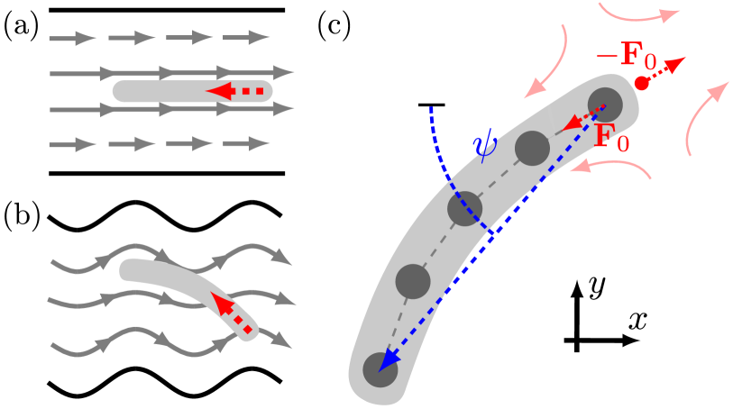
Figure 1: (a) A flexible swimmer (light gray) swims against (red dashed arrow) straight flow lines at the channel center (channel walls black lines, swimmer size enhanced). (b) A wavy channel suppresses rheotaxis. (c) Deformable swimmer (light gray), composed of $N=5$ beads (dark gray) in the $x$-$y$-plane, with its mean orientation angle $\psi$ (blue dashed line). The force dipole at its rear (pair of red arrows) creates a pusher-type flow field (light red dotted arrows) and thrust along the instantaneous swimming direction, given by ${\bf F}_{0}$.

In wavy Poiseuille flows [outlined in Fig. 1(b)] we find a novel resonance for specific flow velocities and channel geometries, resulting in depletion of swinging swimmers from the channel center. Moreover, by the wavy-induced tumbling motion of swimmers, migration to the peripheral attractors is suppressed in a controlled manner.

A semiflexible microswimmer in a Newtonian fluid with viscosity $\eta$ is modeled by $N$ small spheres with radius $a$ at positions ${\bf r}_{i}=(x_{i},y_{i},z_{i})$ ($i=1,...,N$) [cf. Fig. 1(c)], and its center at ${\bf r}_{\text{c}}=\sum_{i=1}^{N}{\bf r}_{i}/N$. The undeformed swimmer is straight with length $L_{0}=(N-1)b+2a$, with equilibrium distance of two neighboring beads $b$. The translational $\dot{{\bf r}}_{i}$ and angular velocities ${\boldsymbol{\Omega}}_{i}$ of each bead are

$$\dot{{\bf r}}_{i}={\bf u}({\bf r}_{i}) +\sum_{j=1}^{N+1}{\boldsymbol{\mu}}_{ij}^{\text{tt}}{\bf F}_{j}+\sum_{j=1}^{N}{\boldsymbol{\mu}}_{ij}^{\text{tr}}{\bf T}_{j},$$

$${\boldsymbol{\Omega}}_{i}=\frac{1}{2}\nabla\times{\bf u}({\bf r}_{i}) +\sum_{j=1}^{N+1}{\boldsymbol{\mu}}_{ij}^{\text{rt}}{\bf F}_{j}+\sum_{j=1}^{N}{\boldsymbol{\mu}}_{ij}^{\text{rr}}{\bf T}_{j}$$ (1)

with the mobility matrices ${\boldsymbol{\mu}}_{ij}$ wajnryb_mizerski_zuk_szymczak_2013 ; zuk_wajnryb_mizerski_szymczak_2014 and bead torques ${\bf T}_{i}$ coupling bead rotations to the swimmer configuration, as given in Ref. supplement . ${\bf u}({\bf r}_{i})$ is the background flow as described below. The bead forces are ${\bf F}_{i}=-\nabla_{i}\left(V_{i}^{\text{H}}+V_{i}^{\text{B}}\right)$ with the harmonic spring potential $V_{i}^{\text{H}}$ and spring constant $k$ between neighboring beads. $V_{i}^{\text{B}}=-\kappa/2\ln\left(1-\cos\alpha_{i}\right)$ is a bending potential PhysRevE.51.2658 with bending rigidity $\kappa$ and opening angle $\alpha_{i}$ of the chain at sphere $i$. We assume an inextensible swimmer with large $k$ and $\kappa$ smaller to allow for bending. Self-propulsion is implemented by a force ${\bf F}_{0}=F_{0}\hat{\bf{e}}_{s}$ acting on the $N$-th bead in the chain with unit vector in swimming direction $\hat{\bf{e}}_{s}:=\left({\bf r}_{N-1}-{\bf r}_{N}\right)/|{\bf r}_{N-1}-{\bf r}_{N}|$. This driving force ${\bf F}_{0}$ is balanced for a force free swimmer by its antiparallel counterpart, $-{\bf F}_{0}$, acting on the counter-force point at ${\bf r}_{N}-2a\hat{\bf{e}}_{s}$. Depending on the sign of $F_{0}$, this pair of forces pushes the bacterial body in front of it and creates the flow field of a pusher ($F_{0}>0$), or drags the body behind it and creates a puller-type flow field ($F_{0}<0$) Elgeti_2015 ; doi:10.1063/1.4944962 . The flow disturbance caused by the counter-force point accounts for the $N+1-$st contribution to the translational and angular velocities in Eq. (1). The swimming speed $v_{0}$ depends linearly on $F_{0}$ supplement . For simplicity, we restrict our analysis to the $x$-$y$ plane and on pushers, as for rod-shaped swimmers like the bacteria E. coli or B. subtilis. The swimmer dynamics is characterized by the angle $\psi$ between its end-to-end vector and the $x$-axis. Pushers and pullers behave similar for large parameter ranges.

We consider a serpentine channel geometry with the same modulation wavelength $\lambda$ and phase for the two opposite walls [cf. Fig. 1(b)] at

$$y_{\text{w}}(x)=d\left[\pm 1+\varepsilon\sin\left(\frac{2\pi x}{\lambda}\right)\right].$$ (2)

Here, $d$ is the channel half-height and $\varepsilon$ the dimensionless modulation amplitude. That is in contrast to channels in Ref. PhysRevLett.122.128002 on cross-stream migration (CSM) of capsules and red blood cells, where modulations of the opposite walls are shifted by half a wavelength. For $\varepsilon\ll 1$, we determine the flow field ${\bf u}({\bf r})=(u_{x},u_{y},0)$ by a perturbation expansion,

$$u_{x}(x,y) = u_{0}\left(1-\frac{y^{2}}{d^{2}}+\varepsilon\ U_{1}(x,y)\right)$$

$$u_{y}(x,y) = u_{0}\varepsilon\ U_{2}(x,y),$$ (3)

with flow amplitude $u_{0}$. The functions $U_{1}(x,y)$ and $U_{2}(x,y)$ are given in supplement and the parameters in parameters_incl_plane .

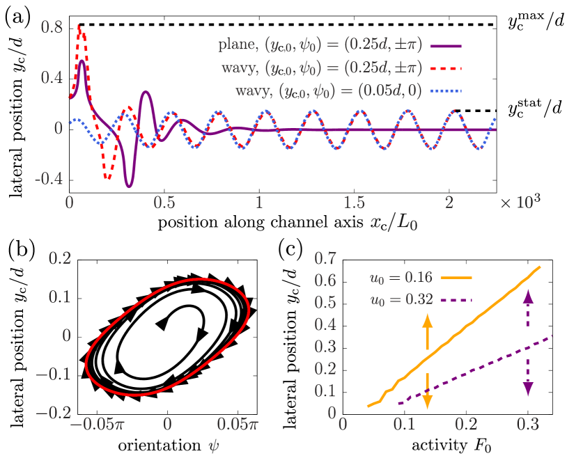
Figure 2: (a): A semiflexible microswimmer with $F_{0}=0.6$ and $\kappa=0.5$ approaches the center of a plane channel along the violet solid trajectory, orienting upstream. In wavy channels this fixed point is replaced by a limit cycle (red dashed and blue dotted lines). Maximum ($y_{\text{c}}^{\text{max}}$) and steady-state amplitude ($y_{\text{c}}^{\text{stat}}$) are also shown. (b): Phase space trajectory (black) in wavy flow for initial conditions $(y_{\text{c},0},\psi_{0})=(0.05d,0)$ and the limit cycle (red). (c): Repeller for tumbling swimmers for $u_{0}=0.16$ (orange solid line) and $u_{0}=0.32$ (violet dashed line). Arrows illustrate the migration direction.

Fig. 2(a) compares trajectories of a semiflexible swimmer in unbounded planar ($\varepsilon=0$) and wavy Poiseuille flow with $\varepsilon=0.1$. In planar Poiseuille flow it first tumbles, then transitions to swinging, and finally approaches the fixed point $(y_{\text{c}},\psi)=(0,0)$ (upstream orientation at the channel center). In a wavy channel, the non-zero flow vorticity causes the swimmer to oscillate periodically about its mean upstream orientation, resulting in a swinging motion. Choosing $u_{0}>v_{0}$, swimmers drift downstream in both planar and wavy flows. The short-time transient in the wavy flow depends on the swimmer’s initial position and orientation, but the long-time behavior does not [cf. red dashed and blue dotted trajectory in Fig. 2(a)]. In the following, we refer to the constant long-time swinging amplitude as $y_{\text{c}}^{\text{stat}}$ and to the maximum of the oscillation during the transient regime as $y_{\text{c}}^{\text{max}}$, as indicated in Fig. 2(a). Fig. 2(b) shows a phase space trajectory for a swimmer starting upstream oriented from a lateral position near the center of the channel that converges to a periodic trajectory (limit cycle).

In planar Poiseuille flow, a rigid swimmer is described by a Hamiltonian system with periodic phase-space orbits that depend on the initial conditions PhysRevLett.108.218104 ; zottl2013periodic . A semiflexible swimmer breaks the periodicity of its trajectory tournus2015flexibility . This results in the inward drift during tumbling and the transition to swinging with a decaying amplitude supplement . Swimmer reorientation against the flow is thus the result of an interplay of its shear-flow induced deformation and self-propulsion $F_{0}$. This inward drift stands in contrast to the outward migration of passive soft particles with elongated shapes, such as flexible fibers and elongated vesicles farutin2016dynamics ; slowicka2013lateral . This type of migration originates from the particle’s hydrodynamic self-interaction and its shear-rate-induced deformation. These two competing migration mechanisms result in a repeller, as shown in Fig. 2(c) that separates outward and inward-directed trajectories. Whereas the mechanism of passive CSM dominates for small $F_{0}$ and large distances from the channel center, the activity-induced inward CSM outweighs the outward CSM for growing $F_{0}$. The repeller for $u_{0}=0.16$ lies above the repeller for $u_{0}=0.32$, since weaker flows result in a larger relative influence of activity.

We now analyze the swimmer behavior in the wavy flow as a function of modulation length $\lambda$ and amplitude $\varepsilon$. We compute $y_{\text{c}}^{\text{stat}}$ by the maximum of the magnitude of $y_{\text{c}}(t)$ beyond the transient regime in $t\in[1,2]\times 10^{6}$. For small oscillations, the swinging frequency of an elongated microswimmer in planar Poiseuille flow is given by $\omega_{0}=\sqrt{u_{0}v_{0}(1-G)}/d$ zottl2013periodic , with geometry factor $G=\left(r_{\text{p}}^{2}-1\right)/\left(r_{\text{p}}^{2}+1\right)$ and swimmer aspect ratio $r_{\text{p}}=1+(N-1)b/(2a)$. An additional frequency $\omega_{\text{Ch}}$ is imposed on the swimmer when it moves along wavy streamlines. Assuming a perfect upstream swimmer orientation yields $\omega_{\text{Ch}}\approx 2\pi|u_{0}-v_{0}|/\lambda$. In our system, $\omega_{0}$ can be interpreted as the oscillator eigenfrequency and $\omega_{\text{Ch}}$ the frequency of an external periodic drive with amplitude $\varepsilon$. We expect the swinging amplitude to peak in the resonance case of $\omega_{\text{Ch}}\approx\omega_{0}$, which determines a resonance wavelength via

$$\lambda_{\text{res}}\approx\frac{2\pi d|u_{0}-v_{0}|}{\sqrt{u_{0}v_{0}\left(1-G\right)}}.$$ (4)

Fig. 3(a) shows the swinging amplitude vs $\lambda$. For small wavelengths, both the initial and steady-state response of the system are small, with $y_{\text{c}}^{\text{stat}}\rightarrow 0$ for $\lambda\rightarrow 0$. This case corresponds to a very large $\omega_{\text{Ch}}$. Increasing $\lambda$ causes increasing maximum and steady-state oscillation amplitudes, culminating in a peak of $y_{\text{c}}^{\text{max}}$ in the range of $193\lesssim\lambda/L_{0}\lesssim 223$ [light red area in Fig. 3(a)]. For these $\lambda$, the transient swimmer response is large enough that one of its beads reaches the wall position. In this case, we stop the simulation in unbounded flows. The influence of repulsive swimmer-wall interactions is discussed below. For further growing $\lambda$, $y_{\text{c}}^{\text{max}}$ and $y_{\text{c}}^{\text{stat}}$ decrease monotonically and approach a small but finite amplitude for large wavelengths.

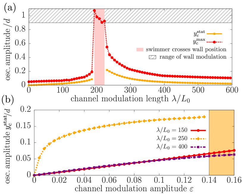
Figure 3: (a): Resonance curve with steady-state ($y_{\text{c}}^{\text{stat}}$, orange bold line, squares) and maximum amplitude ($y_{\text{c}}^{\text{max}}$, red dotted line, circles) vs modulation length $\lambda$ in units of the swimmer length $L_{0}$. Wall modulation for $\varepsilon=0.1$ in the black shaded range. (b): $y_{\text{c}}^{\text{stat}}$ vs modulation amplitude $\varepsilon$ for $\lambda/L_{0}=150$ below (red bold lines, circles) and $\lambda/L_{0}=400$ beyond the resonance wavelength (violet dashed-dotted lines, squares). For $\lambda/L_{0}=250$ (orange dotted lines) the swimmer crosses the wall position in the orange range.

With the parameters listed in parameters_incl_plane , we obtain $\lambda_{\text{res}}\approx 257L_{0}$ from Eq. (4) which is close to the resonance region in Fig. 3(a). The difference between this theoretical prediction and the numerics arises from the assumption of perfect upstream orientation and a constant swimmer position at the channel center. For increasing swinging amplitudes, i.e., for $\lambda\approx\lambda_{\text{res}}$, the swimmer on average visits positions further away from the channel center more often where the flow is slower. Thus, $\omega_{\text{Ch}}$ is effectively smaller than assumed above.

Increasing $\varepsilon$ results in a growing size of the limit cycle, as shown in Fig. 3(b). That applies to $\lambda$ smaller, larger, and close to the $\lambda_{\text{res}}$ [cf. Fig. 3(a)]. In the latter case, we observe crossings of wall positions of the swimmer during the initial transient for $\varepsilon>0.14$. For the effect of activity on the swimmer behavior in the wavy channel see supplement .

Apart from the channel geometry, the experimentally controllable flow strength significantly impacts the swimmer behavior in the wavy channel. We choose $\lambda=150L_{0}$, a wavelength smaller than $\lambda_{\text{res}}$ in Fig. 3(a), and show in Fig. 4 the steady-state swinging amplitude vs the normalized flow amplitude for different rigidities $\kappa=1,3$.

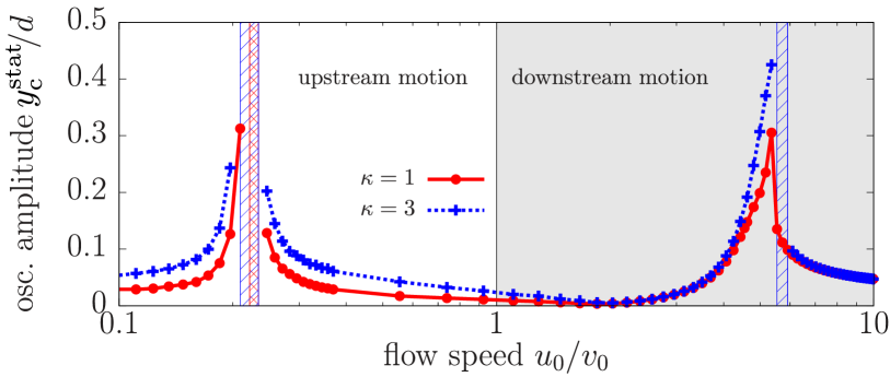
Figure 4: The steady-state swinging amplitude $y_{\text{c}}^{\text{stat}}/d$ vs velocity ratio $u_{0}/v_{0}$ is larger for stiffer swimmers ($\kappa=3$, blue dotted lines, crosses) than for softer ones ($\kappa=1$, red bold lines, circles), with upstream (white, left panel) and downstream resonance (gray, right panel). The swimmer exceeds the wall position in certain ranges of $u_{0}/v_{0}$ (blue dashed boxes for $\kappa=3$ and red double-dashed box for $\kappa=1$).

We observe resonant behavior for both upstream ($u_{0}<v_{0}$) and downstream motion ($u_{0}>v_{0}$). Depending on $\kappa$, the resonant oscillations can become large enough to trigger a crossing of one of the channel wall positions. Flow speed ranges above and below the respective resonance ratio $u_{0}/v_{0}$ are characterized by a comparably small $y_{\text{c}}^{\text{stat}}$. Assuming fixed $\lambda$, we solve Eq. (4) for $u_{0}/v_{0}$, yielding

$$\frac{u_{0}}{v_{0}}=1+\frac{\alpha^{2}}{2}\left(1-G\right)\pm\alpha\sqrt{\left(1-G\right)+\frac{\alpha^{2}}{4}\left(1-G\right)^{2}},$$ (5)

where $\alpha:=\lambda/(2\pi d)>0$ depends only on the channel’s geometry. Eq. (5) has the two solutions $u_{0}/v_{0}=4.54$ (downstream drift) and $u_{0}/v_{0}=0.22$ (upstream swimming). Both give a good approximation for the location of the numerically obtained maxima in Fig. 4. Our predictions for $\omega_{0}$ and $\omega_{\text{Ch}}$ agree well with the numerically obtained Fourier spectra of the swimmer trajectory supplement .

We now include a short-range repulsive wall potential doi:10.1063/1.1674820 in our simulations, as described in supplement . For a large ratio $u_{0}/v_{0}=107$ we find in plane channels a repeller at $y\approx\pm d/4$. Swimmers beyond the repeller migrate closer to the wall and then tumble around a constant $y$-position [blue bold trajectory in Fig. 5(a)].

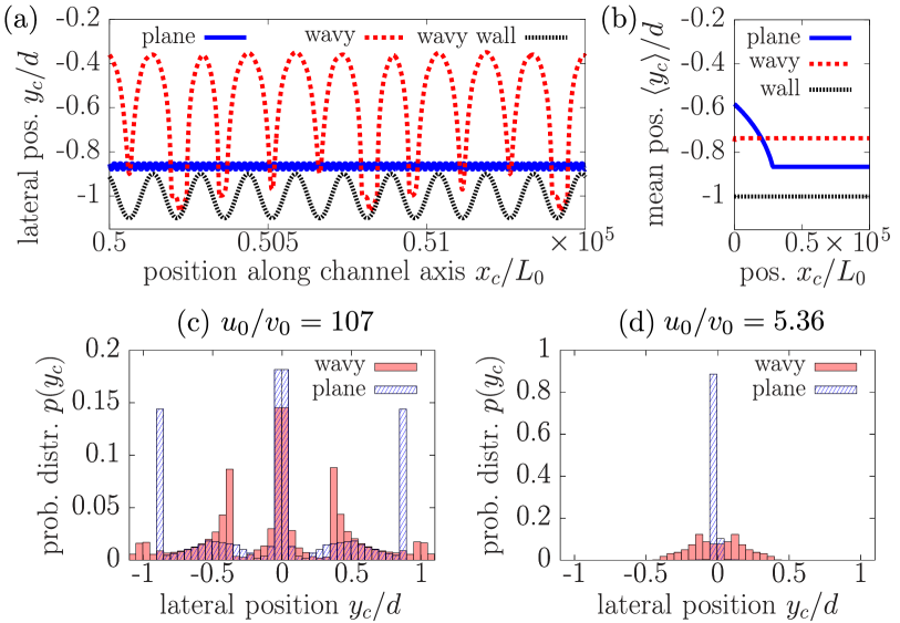
Figure 5: (a) Individual and (b) mean trajectories for a swimmer starting at $y_{c,0}=-0.6d$ in straight (blue bold line) and wavy streamlines (red dashed line) with $u_{0}=107v_{0}$. Black dotted line is the wavy channel boundary in (a) and its mean at $y_{\text{w}}=-1$ in (b). (c) Probability distribution $p(y_{c})$ of a swimmer in straight (dashed blue bars) and wavy streamlines (bold red bars) for $u_{0}/v_{0}=107$ and in (d) for $u_{0}/v_{0}=5.36$.

In wavy flows, tumbling has a much larger amplitude and a periodicity of $4\lambda$ [red dashed trajectory in Fig. 5(a)]. Fig. 5(b) shows swimmer trajectories averaged over $4\lambda$ on a longer time scale. One finds an initial outward drift in plane flows, whereas no drift occurs in wavy channels, where $\langle y_{c}\rangle$ is closer to the center for large times. In plane flows, the swimmer migrates by a lateral distance of $0.32d$ while traveling $2.9\times 10^{4}L_{0}$ in $x$-direction [blue bold trajectory in Fig. 5(b)]. By contrast, lateral motion in wavy flows is faster: The large tumbling amplitude enables the swimmer to move up to $0.71d$ in $y$-direction while being advected downstream only $86L_{0}$.

Figs. 5(c) and (d) show the lateral probability distribution $p(y_{\text{c}})$ for large $u_{0}/v_{0}$ and a $20$ times smaller ratio, $u_{0}/v_{0}=5.36$. We obtain $p(y_{\text{c}})$ by averaging individual swimmer distributions for $10$ different initial positions $y_{c,0}\in[-d/2,d/2]$. Each individual distribution is determined during the simulation time $t_{\text{end}}=3\times 10^{7}$. The repeller causes swimmers in plane channels to accumulate for larger $u_{0}/v_{0}$ either at their center or at an attractor close to each wall [three peaks in Fig. 5(c)]. The small probabilities between the peaks of $p(y_{\text{c}})$ result from the transient CSM to the attractors. By contrast, in wavy channels the large tumbling amplitude shown in Fig. 5(a) leads to small values of $p(y_{\text{c}})$ near the walls even for a large velocity ratio. For smaller $u_{0}/v_{0}$, swimmers migrate to the center of plane channels for all initial positions, resulting in a single peak of $p(y_{\text{c}})$ at $y_{\text{c}}=0$ in Fig. 5(d). This behavior is changed in wavy flows where the above described swinging motion [see Fig. 2(a)] broadens $p(y_{\text{c}})$ and reduces the swimmer probability at the channel center significantly.

In this work we analyzed the behavior of elongated semiflexible microswimmers, such as bacteria, in flows through both plane and wavy microchannels. In planar channels, at lower flow velocities, swimmers concentrate at their center while orienting upstream. At higher flow velocities, we predict two additional attractors closer to the walls for tumbling swimmers, which coexist with the attractor at the channel center. The proximity of the attractors to the walls may promote the formation of bacterial biofilms at the boundaries flemming2016biofilms as well as upstream migration due to surface rheotaxis PhysRevLett.98.068101 ; KAYA20121514 . This is suppressed by wavy boundaries which lead to swimmer depletion close to the walls. For certain ranges of the ratio of the flow strength to swimming speed, we discovered a resonance effect induced by the wavy streamlines. This and the associated swinging/tumbling motion can be controlled by the flow velocity, the swimmer’s speed and size, and the boundary modulation. Thereby swimmers cross the entire channel periodically and the probability distribution becomes broad. This can, for example, prevent the formation of swimmer clusters PhysRevE.90.063019 . In addition, near the resonance, bacteria are forced to hit the walls where they can be killed, e.g., by nanopillars michalska2018tuning or antibacterial surface coatings vasilev2009antibacterial . We expect hydrodynamic swimmer-wall interactions kurzthaler_stone to affect our results quantitatively, but not fundamentally. Possible emergent behavior due to noise effects ezhilan_saintillan_2015 ; PhysRevResearch.2.033275 and chirality of flagella mathijssen2019oscillatory are the subject of future studies.

W.S. thanks for support DAAD, W.S. and W.Z. the French-German University (Grant No. CFDA-Q1-14, “Living fluids”) and the Elite Study Program Biological Physics, and A. Förtsch and M. Laumann for inspiring discussions. The research of I.S.A. was supported by the NSF awards PHY-2140010.

References

- (1) R. Rusconi, J. S. Guasto, and R. Stocker, Nat. Phys. 10, 212 (2014).
- (2) G. L. Miño et al., Adv. Microbiol. 8, 451 (2018).
- (3) G. Junot et al., EPL 126, 44003 (2019).
- (4) A. J. Mathijssen et al., Nat. Commun. 10, 1 (2019).
- (5) N. Figueroa-Morales et al., Sci. Adv. 6, (2020).
- (6) F. P. Bretherton and N. M. V. Rothschild, Proc. Roy. Soc. B 153, 490 (1961).
- (7) K. Miki and D. E. Clapham, Curr. Biol. 23, 443 (2013).
- (8) V. Kantsler, J. Dunkel, M. Blayney, and R. E. Goldstein, Elife 3, e02403 (2014).
- (9) A. Bukatin et al., Proc. Natl. Acad. Sci. (USA) 112, 15904 (2015).
- (10) N. Waisbord, A. Dehkharghani, and J. S. Guasto, Nat. Commun. 12, 1 (2021).
- (11) J. Palacci et al., Sci. Adv. 1, (2015).
- (12) L. Ren et al., ACS Nano 11, 10591 (2017).
- (13) W. Uspal, M. N. Popescu, S. Dietrich, and M. Tasinkevych, Soft Matter 11, 6613 (2015).
- (14) Q. Brosseau et al., Phys. Rev. Lett. 123, 178004 (2019).
- (15) R. Baker et al., Nanoscale 11, 10944 (2019).
- (16) L. D. Rubio et al., Adv. Intell. Syst. 3, 2000178 (2021).
- (17) A. Zöttl and H. Stark, Phys. Rev. Lett. 108, 218104 (2012).
- (18) A. Zöttl and H. Stark, Eur. Phys. J. E 36, 4 (2013).
- (19) S. Uppaluri et al., Biophys. J. 103, 1162 (2012).
- (20) S. Wang, H. Arellano-Santoyo, P. A. Combs, and J. W. Shaevitz, Proc. Acad. Natl. Sci. (USA) 107, 9182 (2010).
- (21) Y. Caspi, PLOS ONE 9, 1 (2014).
- (22) H. Wada and R. R. Netz, Phys. Rev. Lett. 99, 108102 (2007).
- (23) M. Tournus, A. Kirshtein, L. V. Berlyand, and I. S. Aranson, J. R. Soc. Interface 12, 20140904 (2015).
- (24) M. Kumar and A. M. Ardekani, Soft Matter 15, 6269 (2019).
- (25) M. Potomkin, M. Tournus, L. Berlyand, and I. Aranson, J. R. Soc. Interface 14, 20161031 (2017).
- (26) A. Farutin et al., Soft Matter 12, 7307 (2016).
- (27) A. M. Słowicka, E. Wajnryb, and M. L. Ekiel-Jeżewska, Eur. Phys. J. E 36, 31 (2013).
- (28) B. Kaoui et al., Phys. Rev. E 77, 021903 (2008).
- (29) L. G. Leal, Annu. Rev. Fluid Mech. 12, 435 (1980).
- (30) M. Laumann et al., EPL 117, 44001 (2017).
- (31) E. Wajnryb, K. A. Mizerski, P. J. Zuk, and P. Szymczak, J. Fluid Mech. 731, R3 (2013).
- (32) P. J. Zuk, E. Wajnryb, K. A. Mizerski, and P. Szymczak, J. Fluid Mech. 741, R5 (2014).
- (33) See Supplemental Material at [URL] for the full equations of motion, a validation of the swimmer model including its behavior in linear shear and plane Poiseuille flow, the dependence of the intrinsic swimming speed on the activity, the analytical derivation of the wavy flow and resonance curves for different activities.
- (34) J. Hendricks, T. Kawakatsu, K. Kawasaki, and W. Zimmermann, Phys. Rev. E 51, 2658 (1995).
- (35) J. Elgeti, R. G. Winkler, and G. Gompper, Rep. Prog. Phys. 78, 056601 (2015).
- (36) J. de Graaf et al., J. Chem. Phys. 144, 134106 (2016).
- (37) M. Laumann et al., Phys. Rev. Lett. 122, 128002 (2019).
-
(38)
Simulation parameters for plane flows: Time step , maximum
flow speed , channel half height , fluid viscosity ,
number of beads , equilibrium distance of two neighboring beads , bead radius (aspect ratio , geometry
factor ), activity (intrinsic swimming speed ), harmonic spring stiffness , bending rigidity
, torque strength , initial swimmer
orientation , initial swimmer lateral position . The
migration direction is determined by the sign of the migration velocity which
is obtained by a linear fit to for .
Simulation parameters in wavy flows: Activity (intrisic swimming speed ), bending rigidity , dimensionless modulation amplitude , modulation length , initial swimmer orientation , initial swimmer position , simulation time for each trajectory . Remaining parameters as in simulations in plane flows. - (39) A. Zöttl and H. Stark, Eur. Phys. J. E 36, 1 (2013).
- (40) J. D. Weeks, D. Chandler, and H. C. Andersen, J. Chem. Phys. 54, 5237 (1971).
- (41) H.-C. Flemming et al., Nat. Rev. Microbiol. 14, 563 (2016).
- (42) J. Hill, O. Kalkanci, J. L. McMurry, and H. Koser, Phys. Rev. Lett. 98, 068101 (2007).
- (43) T. Kaya and H. Koser, Biophys. J. 102, 1514 (2012).
- (44) L. Jibuti et al., Phys. Rev. E 90, 063019 (2014).
- (45) M. Michalska et al., Nanoscale 10, 6639 (2018).
- (46) K. Vasilev, J. Cook, and H. J. Griesser, Expert Rev. Med. Devices 6, 553 (2009).
- (47) C. Kurzthaler and H. A. Stone, Soft Matter, 17, 3322 (2021).
- (48) B. Ezhilan and D. Saintillan, J. Fluid Mech. 777, 482–522 (2015).
- (49) K. Qi, H. Annepu, G. Gompper, and R. G. Winkler, Phys. Rev. Res. 2, 033275 (2020).