Understanding the Sources of Error in MBAR through Asymptotic Analysis

Abstract

Multiple sampling strategies commonly used in molecular dynamics, such as umbrella sampling and alchemical free energy methods, involve sampling from multiple thermodynamic states. Commonly, the data are then recombined to construct estimates of free energies and ensemble averages using the Multistate Bennett Acceptance Ratio (MBAR) formalism. However, the error of the MBAR estimator is not well-understood: previous error analysis of MBAR assumed independent samples and did not permit attributing contributions to the total error to individual thermodynamic states. In this work, we derive a novel central limit theorem for MBAR estimates. This central limit theorem yields an error estimator which can be decomposed into contributions from the individual Markov chains used to sample the states. We demonstrate the error estimator for an umbrella sampling calculation of the alanine dipeptide in two dimensions and an alchemical calculation of the hydration free energy of methane. In both cases, the states’ individual contributions to the error provide insight into the sources of error of the simulations. Our numerical results demonstrate that the time required for the Markov chain to decorrelate in individual thermodynamic states contributes considerably to the total MBAR error. Moreover, they indicate that it may be possible to use the contributions to tune the sampling and improve the accuracy of MBAR calculations.

I Introduction

Molecular dynamics simulations provide a means to compute key quantities in statistical mechanics, typically in the form of ensemble averages of certain observables. In principle, it is possible to estimate ensemble averages by running a long, unbiased simulation of a system and averaging over the resulting trajectory. However, in practice this can be inefficient. For instance, the determination of the relative free energy is of particular interest since the free energy is the fundamental quantity that determines the spontaneity of thermodynamic processes and the accessibility of thermodynamic states. However, the ensemble averages required for estimating free energies are notoriously slow to converge and typically require simulations to explore multiple regions of a system’s configurational spaceChipot and Pohorille (2007); Lelièvre, Rousset, and Stoltz (2010).

A common strategy for addressing this problem is to sample from multiple thermodynamic states. If the states are chosen well, ensemble averages will converge much more quickly in these new statesDinner et al. (2020). This approach is the basis of multiple simulation strategies such as umbrella sampling, parallel tempering, and alchemical free energy simulation. Umbrella sampling enforces sampling of the conformational changes of biomolecular systems by running a series of independent simulations, each biased to sample a different region of a physical system’s phase spaceTorrie and Valleau (1977); Pangali, Rao, and Berne (1979). Parallel tempering simulates several replicas of a system with the same Hamiltonian but at different temperatures to allow the system to cross over energetic barriersSwendsen and Wang (1986); Geyer (1991). Alchemical free energy calculations of molecular systems estimate the free energy difference between two molecular states by interpolating between their HamiltoniansTembre and Mc Cammon (1984); Frenkel and Smit (2002); Chodera et al. (2011). In all of these cases, data sampled from multiple thermodynamic states must be combined to obtain the averages of interest.

A popular algorithm for doing this is the Multistate Bennett Acceptance Ratio (MBAR)Shirts and Chodera (2008), originally derived in Vardi, 1985. For statistically independent samples, MBAR combines the data across states in a statistically optimal manner. Although molecular dynamics simulations are correlated, MBAR nevertheless achieves good results in practice. However, solving for the MBAR estimate involves solving a nonlinear fixed point problem which complicates error analysis. Previous attempts to construct error estimates have explicitly assumed that samples are statistically independentKong et al. (2003); Shirts and Chodera (2008), which is typically not true for molecular dynamics data.

In the present paper, we build on Thiede et al., 2016; Dinner et al., 2020 to derive a formal expression for the asymptotic variance of the MBAR estimator that explicitly accounts for correlation in sampled data. Moreover, our estimator can be decomposed into error contributions from individual states. This can potentially give practitioners insight into how sampling in individual thermodynamic states affects global error, and may lead to adaptive sampling strategies to accelerate convergence.

II Background on Monte Carlo and Asymptotic Error

Many fundamental quantities in statistical mechanics take the form of high-dimensional integrals. Physical theories often require estimating averages over a physical system’s Boltzmann distribution of the form

$$\left\langle g\right\rangle=\frac{\int g(x)e^{-H(x)/k_{B}T}dx}{\int e^{-H(x)/k_{B}T}dx},$$ (1)

where $H$ is the system’s Hamiltonian and $x$ is its configuration in $\mathbb{R}^{n}$. Alternatively, they may require estimates of the free energy difference between two regions of phase space:

$$\Delta G_{A\to B}= -k_{B}T\log\frac{\int\mathds{1}_{B}(x)e^{-H(x)/k_{B}T}dx}{\int\mathds{1}_{A}(x)e^{-H(x)/k_{B}T}dx}$$ (2)

$$= -k_{B}T\log\frac{\left\langle\mathds{1}_{B}\right\rangle}{\left\langle\mathds{1}_{A}\right\rangle},$$ (3)

where $\mathds{1}_{D}(x)$ is $1$ if the configuration $x$ is in a region labeled $D$ and $0$ otherwise. We might also wish to estimate the free energy difference between two Hamiltonians, given by

$$\Delta G_{\alpha\to\beta}=-k_{B}T\log\frac{\int e^{-H_{\beta}(x)/k_{B}T}dx}{\int e^{-H_{\alpha}(x)/k_{B}T}dx}.$$ (4)

For most systems, these integrals are too complex to be evaluated analytically, and the dimension of $x$ is too high to use quadrature. Instead, they are typically treated by Monte Carlo methods.

II.1 Markov chain Monte Carlo

Assume that we are given a probability distribution with an unnormalized density $q$ over the Lebesgue measure on $\mathbb{R}^{n}$. For instance, in statistical mechanics $q$ is typically the Boltzmann factor:

$$q(x)=e^{-H(x)/k_{B}T}.$$ (5)

We can then write the average of a function $g:\mathbb{R}^{n}\to\mathbb{R}$ over the distribution as

$$\left\langle g\right\rangle=\frac{\int g(x)q(x)dx}{c},\qquad c=\int q(x)dx.$$ (6)

In statistical mechanics, we refer to these averages as ensemble averages. Particular choices of $g$ allow us to rewrite key quantities in statistical mechanics as ensemble averages. Substituting the Boltzman factor for $q$ directly recovers (1), and the free energy differences between regions of phase space in (3) is merely the ratio between two averages. Similarly, to estimate the free energy difference between two Hamiltonians, we can set $q$ to $\exp\left(-H_{\alpha}/k_{B}T\right)$ and rewrite (4) as

$$e^{-\Delta G_{\alpha\to\beta}/k_{B}T}=\left\langle e^{-\left(H_{\beta}(x)-H_{\alpha}(x)\right)/k_{B}T}\right\rangle.$$ (7)

Monte Carlo methods approximate ensemble averages by drawing a sequence of $N$ samples $\left\{X_{t}\right\}$ from the probability distribution and averaging over them. If the sampling procedure is chosen appropriately, we expect sample averages to converge to the true (ensemble) average over $p$.

$$\bar{g}=\frac{1}{N}\sum_{t=0}^{N-1}g\left(X_{t}\right)\xrightarrow{a.s.}\left\langle g\right\rangle.$$ (8)

Here $a.s.$ denotes almost sure convergence, a strong form of probabilistic convergence. (Specifically, the probability of $\bar{g}$ not converging to $\left\langle g\right\rangle$ is zero.) If the samples are statistically independent we say that our samples are independent and identically distributed (IID), and (8) is guaranteed to hold by the Law of Large NumbersLelièvre, Rousset, and Stoltz (2010). However, in practice it is often impossible to generate IID samples, and we must instead generate samples by running a Markov chain that has $p$ as its stationary distribution: a practice known as Markov chain Monte Carlo (MCMC). Then, (8) still holds if the Markov chain is ergodic Lelièvre, Rousset, and Stoltz (2010).

II.2 Asymptotic Variance of Monte Carlo Estimates

While (8) guarantees that the error goes to zero as the number of samples increases, it says nothing about how quickly this happens. A common method to quantify how the sampling error decreases increasing sample size is to use a Central Limit Theorem (CLT): a theorem showing that a sequence of random variables converges to a known normal distributionLelièvre, Rousset, and Stoltz (2010). Specifically, assume that we wish to evaluate the ensemble average of several functions, each denoted $g_{i}$. Concatenating our sample means and ensemble averages into vectors we denote as $\bar{\mathbf{g}}$ and $\left\langle\mathbf{g}\right\rangle$ respectively, we can often show that the error between the two converges to a multivariate normal (Gaussian) distribution when appropriately scaled:

$$\sqrt{N}\left(\bar{\mathbf{g}}-\left\langle\mathbf{g}\right\rangle\right)\xrightarrow{d}\mathbf{N}\left(0,\Sigma\right).$$ (9)

Here $\mathbf{N}$ denotes a normal (Gaussian) random variable with mean vector $\mu$ and covariance matrix $\Sigma$, known as the asymptotic covariance. The symbol $\xrightarrow{d}$ denotes convergence in distribution (a weaker form of probabilistic convergence than almost sure convergence). For IID samples, (9) holds for all functions with finite variance and $\Sigma_{ij}$ is simply the covariance between $g_{i}$ and $g_{j}$ over $p$. If samples are instead gathered from a Markov chain $X_{t}$, proving a CLT requires more technical conditions on the nature of the Markov Chain and $\mathbf{g}$ Chan (1993); Tierney (1994); Geyer and Chan (1994); Jones (2004). However, for most commonly used Markov chains and most reasonable applications, we can expect (9) to hold. In this case, if the Markov chain is time-homogeneous (i.e., the rule for updating the Markov chain is the same at all times) with ergodic distribution $p$, the asymptotic covariance matrix is given by

$$\Sigma_{ij}=\operatorname{cov}\{g_{i}(X_{t}),g_{j}(X_{t})\}+2\sum_{k=1}^{\infty}\operatorname{cov}\{g_{i}(X_{t}),g_{j}(X_{t+k})\},$$ (10)

where in this formula (and only this formula) we assume that the chain is stationary with $X_{t}$ distributed according to $p$ for all $t$.

The CLT and the asymptotic covariance help diagnose the error and convergence of a Markov chain Monte Carlo simulation. For example, under mild technical conditions (specifically geometric ergodicity and bounded $g$), $\Sigma_{ii}/N$ is asymptotic to $\operatorname{var}\{\bar{g}_{i}\}$. Consequently, we can treat $\sqrt{\Sigma_{ii}/N}$ as a rough estimate for the error in using $\bar{g}_{i}$ to estimate of $\langle g_{i}\rangle$. The sampling efficiency of the Markov chain relative to IID sampling from $p$ can be quantified by the autocorrelation time:

$$\tau_{g_{i}}=\frac{\Sigma_{ii}}{\operatorname{var}\left\{g_{i}\right\}}.$$ (11)

Equivalently,

$$\Sigma_{ii}=\tau_{g_{i}}\operatorname{var}\left\{g_{i}\right\}.$$

Since $\operatorname{var}\left\{g_{i}\right\}/N$ is the variance for IID sampling, we can interpret the autocorrelation time as how many MCMC samples are required to achieve the same reduction in error as a single IID sampleLelièvre, Rousset, and Stoltz (2010); Frenkel and Smit (2002).

III The MBAR Equations

In the previous section, we considered sampling from a single distribution. However, we may often have samples collected from multiple, related probability distributions. For concreteness, assume we have $L$ probability distributions, each with an unnormalized probability density $q_{i}$. We refer to these distributions as states. The ensemble average of an observable $g(x)$ in each state is given by

$$\left\langle g\right\rangle_{i}=\frac{\int g(x)q_{i}(x)dx}{c_{i}},\quad c_{i}=\int q_{i}(x)dx.$$ (12)

Here the constant $c_{i}$ is the normalization constant for $q_{i}$. If $q_{i}$ is a Boltzmann distribution, then $c_{i}$ is the corresponding partition function. Next, we assume that for every state we have collected a set of $N_{i}$ samples, denoted $\{X^{i}_{t}\}$. We can then approximate $\left\langle g\right\rangle_{i}$ by the sample average

$$\left\langle g\right\rangle_{i}\approx\frac{1}{N_{i}}\sum_{t=1}^{N_{i}}g(X_{t}^{i})$$

However, if the states have shared regions with high probability, we can construct improved estimates of (12) by using data from all of the states, not just state $i$. This is the aim of the MBAR algorithmVardi (1985); Shirts and Chodera (2008). Following the treatment in Ref. Geyer, 1994, we observe that we can view the union of the samples from the states as samples from a combined distribution known as a mixture distribution. Let

$$N=\sum_{i=1}^{L}N_{i}$$

be the total sample size, and let

$$\kappa_{i}=\frac{N_{i}}{N}$$

be the fraction of sample points collected in state $i$. To simplify the presentation, we will assume that $\kappa_{i}$ is constant and always greater than zero. (A version of our main result that relaxes this assumption is given in the supplement.) We define the mixture distribution to be

$$\pi_{\text{mix}}(x)=\sum_{i=1}^{L}\kappa_{i}q_{i}(x)/c_{i}.$$ (13)

We can then write

$$\left\langle g\right\rangle_{i} =\int\frac{g(x)q_{i}(x)/c_{i}}{\pi_{\text{mix}}(x)}\pi_{\text{mix}}(x)dx$$

$$=\int\frac{g(x)q_{i}(x)/c_{i}}{\sum_{k=1}^{L}\kappa_{k}q_{k}(x)/c_{k}}\sum_{j=1}^{L}\kappa_{j}q_{j}(x)/c_{j}dx$$ (14)

$$=\sum_{j=1}^{L}\kappa_{j}\left\langle\frac{gq_{i}/c_{i}}{\sum_{k=1}^{L}\kappa_{k}q_{k}/c_{k}}\right\rangle_{j}.$$ (15)

In general, the normalization constants for the states are not known. We therefore rewrite (15) in terms of the states’ (unitless) relative free energies, which we denote $f_{i}$. We arbitrarily set the average free energy to be zero, so

$$\frac{1}{L}\sum_{i=1}^{L}f_{i}=0,$$ (16)

and therefore the free energies are defined by

$$f_{i}=-\log c_{i}+\frac{1}{L}\sum_{j=1}^{L}\log c_{j}.$$ (17)

Dividing both the numerator and denominator of (15) by $\exp(-(1/L)\sum_{i=1}^{L}f_{i})$, after a few manipulations we have

$$\left\langle g\right\rangle_{i}=\sum_{j=1}^{L}\kappa_{j}\left\langle\frac{gq_{i}e^{f_{i}}}{\sum_{k=1}^{L}\kappa_{k}q_{k}e^{f_{k}}}\right\rangle_{j}.$$ (18)

This equation can be used to estimate $\left\langle g\right\rangle_{i}$ if we are given an estimate of the free energies, $\bar{f}$. Replacing each ensemble average on the right-hand side with a Monte Carlo estimate we have

$$\bar{g}_{i}=\sum_{j=1}^{L}\frac{\kappa_{j}}{N_{j}}\sum_{t=1}^{N_{j}}\frac{g(X_{t}^{j})q_{i}(X_{t}^{j})e^{\bar{f}_{i}}}{\sum_{k=1}^{L}\kappa_{k}q_{k}(X_{t}^{j})e^{\bar{f}_{k}}}.$$ (19)

This estimator uses data from every state, not just state $i$. Moreover, we can also use (18) to estimate the free energies themselves. Since the ensemble average of the function $g(x)=1$ is always $1$,

$$1= \sum_{j=1}^{L}\kappa_{j}\left\langle\frac{q_{i}e^{f_{i}}}{\sum_{k=1}^{L}\kappa_{k}q_{k}e^{f_{k}}}\right\rangle_{j}$$ (20)

$$\implies f_{i}= -\log\sum_{j=1}^{L}\kappa_{j}\left\langle\frac{q_{i}}{\sum_{k=1}^{L}\kappa_{k}q_{k}e^{f_{k}}}\right\rangle_{j}.$$ (21)

One can thus estimate the free energy by defining $\bar{f}$ to be the solution to

$$\bar{f}_{i}=-\log\left(\sum_{j=1}^{L}\frac{\kappa_{j}}{N_{j}}\sum_{t=1}^{N_{j}}\frac{q_{i}(X_{t}^{j})}{\sum_{k=1}^{L}\kappa_{k}q_{k}(X_{t}^{j})e^{\bar{f}_{k}}}\right).$$ (22)

Not only can this equation can be solved using standard root-finding methods such as Newton-Raphson and gradient descentShirts and Chodera (2008), but there exist rapid algorithms for solving it through a succession of estimation tasksMeng and Wong (1996); Thiede et al. (2016); Dinner et al. (2020). Equations (19) and (22) are the MBAR estimates of the ensemble average and the free energies, respectivelyShirts and Chodera (2008). With sufficient overlap of the samples from different states, (21) uniquely determines $f$. Specifically, if the matrix $M_{ij}=\left\langle q_{i}\right\rangle_{j}$ is irreducible, then by Theorem 1 in Ref. Geyer, 1994 or Proposition 1.1 in Ref. Gill, Vardi, and Wellner, 1988 the $f_{i}$ are uniquely specified by (21). An analogous statement holds for $\bar{f}$. When $M$ is irreducible, Theorem 1.1 in Ref. Gill, Vardi, and Wellner, 1988 implies that equation (22) almost surely has a unique solution $\bar{f}$ when the total sample size $N$ is sufficiently large. Moreover, the estimates of the free energies and the ensemble averages converge to the true values as $N$ increases. To be precise, $\bar{f}_{i}\xrightarrow{a.s.}f_{i}$ and $\bar{g}_{i}\xrightarrow{a.s.}\langle g\rangle_{i}$ by Theorem 1 in Ref. Geyer, 1994.

III.1 Estimating Chemical Quantities using MBAR

Specific manipulations of state free energies and ensemble averages allow us to reconstruct quantities of interest in a broad range of contexts. Here, we discuss the analysis of data from three common algorithms: parallel tempering, alchemical free energy simulations, and umbrella sampling.

In parallel tempering, we seek to estimate ensemble averages for a system with unnormalized probability density

$$e^{-H(x)/k_{B}T}.$$ (23)

However, this density may be highly multimodal, making the probability distribution difficult to sample. Parallel tempering addresses this by running multiple copies of the system with the same Hamiltonian but different temperaturesSwendsen and Wang (1986); Geyer (1991). We write their distributions as

$$q_{i}(x)=e^{-H(x)/k_{B}(T+\delta T_{i})}$$ (24)

One copy, here arbitrarily chosen to have index 1, is set to be at the original temperature (i.e., $\delta T_{1}=0$) and all other copies have $\delta T_{i}\neq 0$. The copies then periodically swap molecular configurations via Monte Carlo moves on the space of copies. In principle, one can estimate averages over (23) by averaging over all configurations collected from $q_{1}$. However, using the MBAR estimator (19) allows one to use data from all states, giving a more accurate answer.

In alchemical free energy simulations, we seek to estimate the free energy difference between two Hamiltonians as in (4)Tembre and Mc Cammon (1984); Frenkel and Smit (2002); Chodera et al. (2011). However, rather than sampling only the state with $H_{\alpha}$, we sample a set of $L$ states that interpolate between $H_{\alpha}$ and $H_{\beta}$. A simple choice would be to set

$$-k_{B}T\log q_{i}=H_{\alpha}+\lambda\left(\frac{i-1}{L-1}\right)(H_{\beta}-H_{\alpha})$$ (25)

where $\lambda:\left[0,1\right]\to\left[0,1\right]$ is a monotonic function such that $\lambda(0)=0$ and $\lambda(1)=1$, although in practice, more complex interpolations are often required Simonson (1993); Beutler et al. (1994); Steinbrecher, Mobley, and Case (2007). With this set of state definitions, the (unitless) free energy difference between the two Hamiltonians is simply the difference between the free energies of the first and last states.

$$-\log\frac{\int e^{-H_{\beta}(x)/k_{B}T}dx}{\int e^{-H_{\alpha}(x)/k_{B}T}dx}=f_{L}-f_{1}$$ (26)

Consequently, we can solve (22) and estimate the free energy difference as $\bar{f}_{L}-\bar{f}_{1}$.

In umbrella samplingTorrie and Valleau (1977); Pangali, Rao, and Berne (1979) we construct a collection of states

$$q_{i}(x)=\psi_{i}(x)q(x)$$ (27)

by multiplying a density $q$ with a biasing function $\psi_{i}$. We then aim to estimate averages of observables over $q$, such as those in (1) and (3). To estimate these averages over $q$ using MBAR by steps similar to those used to derive (15), we write

$$\frac{\int g(x)q(x)dx}{\int q(x)dx}= \frac{\int g(x)q(x)(\pi_{\text{mix}}(x)/\pi_{\text{mix}}(x))dx}{\int q(x)(\pi_{\text{mix}}(x)/\pi_{\text{mix}}(x))dx}$$

$$= \frac{\int g(x)q(x)\frac{\sum_{j}\kappa_{j}q_{j}(x)e^{f_{j}}}{\sum_{l}\kappa_{l}q_{l}(x)e^{f_{l}}}\,dx}{\int q(x)\frac{\sum_{k}\kappa_{k}q_{k}(x)e^{f_{k}}}{\sum_{m}\kappa_{m}q_{m}(x)e^{f_{m}}}\,dx}$$

$$= \frac{\sum_{j=1}^{L}\kappa_{j}\left\langle{gq}/{(\sum_{l=1}^{L}\kappa_{l}q_{l}e^{f_{l}})}\right\rangle_{j}}{\sum_{k=1}^{L}\kappa_{k}\left\langle{q}/{(\sum_{m=1}^{L}\kappa_{m}q_{m}e^{f_{m}})}\right\rangle_{k}}$$

$$= \frac{\sum_{j=1}^{L}\kappa_{j}\left\langle{g}/{(\sum_{l=1}^{L}\kappa_{l}\psi_{l}e^{f_{l}})}\right\rangle_{j}}{\sum_{k=1}^{L}\kappa_{k}\left\langle{1}/{(\sum_{m=1}^{L}\kappa_{m}\psi_{m}e^{f_{m}})}\right\rangle_{k}}.$$ (28)

We can also use umbrella sampling to estimate the difference in free energy between two states. Comparing to (3) and setting $q$ to be the Boltzmann factor, we have

$$\Delta G_{A\to B}= -k_{B}T\log\frac{\int\mathds{1}_{B}(x)e^{-H(x)/k_{B}T}dx}{\int\mathds{1}_{A}(x)e^{-H(x)/k_{B}T}dx}$$

$$= -k_{B}T\log\frac{\sum_{j=1}^{L}\kappa_{j}\left\langle{\mathds{1}_{A}q}/{(\sum_{l=1}^{L}\kappa_{l}q_{l}e^{f_{l}})}\right\rangle_{j}}{\sum_{k=1}^{L}\kappa_{k}\left\langle{\mathds{1}_{B}q}/{(\sum_{m=1}^{L}\kappa_{m}q_{m}e^{f_{m}})}\right\rangle_{k}}$$

$$= -k_{B}T\log\frac{\sum_{j=1}^{L}\kappa_{j}\left\langle{\mathds{1}_{A}}/{(\sum_{l=1}^{L}\kappa_{l}\psi_{l}e^{f_{l}})}\right\rangle_{j}}{\sum_{k=1}^{L}\kappa_{k}\left\langle{\mathds{1}_{B}}/{(\sum_{m=1}^{L}\kappa_{m}\psi_{m}e^{f_{m}})}\right\rangle_{k}},$$ (29)

by steps similar to those for (28).

These examples show how MBAR can be used to efficiently construct estimates from algorithms that collect data in multiple states. Indeed, when IID samples are collected from each state, then MBAR gives the maximum likelihood estimate Vardi (1985) and achieves the best possible mean-squared error in the large-sample limit Shirts and Chodera (2008). MBAR does not give the maximum likelihood estimate for correlated samples, but nevertheless it has been empirically observed to give good results.

However, it is not obvious how to estimate the uncertainty in MBAR averages. In previous work, Kong et al. constructed an estimator for the asymptotic covariance using the Cramer-Rao lower bound of the variance Kong et al. (2003). When samples are uncorrelated, MBAR achieves this lower bound. However, when samples are correlated, this estimator underestimates the asymptotic error. Moreover, the estimator only gives the total asymptotic error and not the contributions from individual thermodynamic states. This makes it difficult to determine how the parameters of individual states contribute to the accuracy of the total simulation. An alternate approach would be to attempt to construct a CLT for MBAR estimates. As discussed in Subsection II.2, CLTs are able to capture the effect of the dynamics on sampling error. Moreover, previous work on other algorithms for recombining data from multiple statesThiede et al. (2016) has shown that CLTs can be used to connect the sampling of individual states to the total error of the estimate. In this work, we establish a CLT for the MBAR equations and show that the resulting error estimates gives detailed insight into how the parameters of multistate simulations contribute to the total error.

IV Asymptotic Variance for the MBAR equations

Here, we give an expression for the asymptotic variance of MBAR estimates of observables and normalization constants. Our approach builds upon the work of GeyerGeyer (1994). Our contribution is essentially to fill in missing details and to correct errors. Most importantly, the formula for the asymptotic variance of observable averages $\bar{g}$ is not correct in Ref. Geyer, 1994.

IV.1 CLTs for the raw output of MBAR

MBAR estimates of observables require calculating the values of $\bar{f}$ as well as one or more empirical averages of the form

$$\bar{\omega}=\sum_{j=1}^{L}\frac{\kappa_{j}}{N_{j}}\sum_{t=1}^{N_{j}}\frac{w(X_{t}^{j})}{\sum_{k=1}^{L}\kappa_{k}q_{k}(X_{t}^{j})e^{\bar{f}_{k}}}$$ (30)

for some function $w:\mathbb{R}^{n}\to\mathbb{R}$. For instance, in (19) we set $w=q_{i}g$ and subsequently multiply by $e^{\bar{f}_{i}}$. The presence of $\bar{f}$ in (30) means that the errors in our observable estimates and in our estimates of the state free energies are correlated. Consequently, we must consider the asymptotic covariance of the free energies and our observables jointly.

To do so, we rewrite (22) and (30) as a single root finding problem. We concatenate the vector of estimated free energies and empirical averages into a single vector

$$\bar{v}=\left(\bar{f}_{1},\ldots,\bar{f}_{L},\bar{\omega}_{1},\ldots,\bar{\omega}_{M}\right).$$ (31)

The vector $\bar{v}$ is the root of the function $\bar{F}:\mathbb{R}^{L+M}\to\mathbb{R}^{L+M}$, where if $i\leq L$

$$\bar{F}_{i}(y)=\kappa_{i}-\sum_{j=1}^{L}\kappa_{j}\frac{1}{N_{j}}\sum_{t=1}^{N_{j}}\frac{\kappa_{i}q_{i}(X_{t}^{j})e^{y_{i}}}{\sum_{k=1}^{L}\kappa_{k}q_{k}(X_{t}^{j})e^{y_{k}}}$$ (32)

and if $i>L$ then

$$\bar{F}_{i}(y)=y_{i}-\sum_{j=1}^{L}\kappa_{j}\frac{1}{N_{j}}\sum_{t=1}^{N_{j}}\frac{w_{i-L}(X_{t}^{j})}{\sum_{k=1}^{L}\kappa_{k}q_{k}(X_{t}^{j})e^{y_{k}}}.$$ (33)

Writing the MBAR estimates as the roots of $\bar{F}$ suggests a strategy for proving a CLT. For any fixed $y$, each element in $\bar{F}(y)$ is a sum of sample averages over our states. It is therefore reasonable to assume the existence of a CLT for each of the sample averages. If we can then convert a CLT for each of the collection of averages into a CLT for the roots of $\bar{F}$, then we have proven a CLT for MBAR estimates. Indeed, this is precisely the strategy we pursue. A full proof of the CLT is given in Section I of the supplement. Here, we merely state introduce the key quantities necessary to state our results and state our result.

We first discuss the asymptotic covariance structure of each of the averages in (33) and (33). For convenience, we define

$$\xi_{i}(x,y)=\begin{cases}\frac{\kappa_{i}q_{i}(x)e^{y_{i}}}{\sum_{k=1}^{L}\kappa_{k}q_{k}(x)e^{y_{k}}}\>\text{if}\;i\leq L\\ \frac{w_{i-L}(x)}{\sum_{k=1}^{L}\kappa_{k}q_{k}(x)e^{y_{k}}}\>\text{if}\;i>L\end{cases}.$$ (34)

We can then write $\bar{F}_{i}(y)$ using a $\kappa_{j}$-weighted sum of ergodic averages of the form

$$\bar{\xi}^{j}_{i}(y)=\frac{1}{N_{j}}\sum_{t=1}^{N_{j}}\xi_{i}(X^{j}_{t},y).$$

In the limit as $N\rightarrow\infty$, $\bar{\xi}^{j}_{i}(y)$ converges to

$$\xi^{j}_{i}(y)=\begin{cases}\left\langle\frac{\kappa_{i}q_{i}e^{y_{i}}}{\sum_{k=1}^{L}\kappa_{k}q_{k}e^{y_{k}}}\right\rangle_{j}\quad\text{if}\quad i\leq L\\ \left\langle\frac{w_{i-L}}{\sum_{k=1}^{L}\kappa_{k}q_{k}e^{y_{k}}}\right\rangle_{j}\quad\text{if}\quad i>L,\end{cases}$$

and $\bar{F}$ converges to

$$F_{i}(y)=\begin{cases}\kappa_{i}-\sum_{j=1}^{L}\kappa_{j}\left\langle\frac{\kappa_{i}q_{i}e^{y_{i}}}{\sum_{k=1}^{L}\kappa_{k}q_{k}e^{y_{k}}}\right\rangle_{j}\quad\text{if}\quad i\leq L\\ y_{i}-\sum_{j=1}^{L}\kappa_{j}\left\langle\frac{w_{i-L}}{\sum_{k=1}^{L}\kappa_{k}q_{k}e^{y_{k}}}\right\rangle_{j}\quad\text{if}\quad i>L.\end{cases}$$ (35)

We assume that a central limit theorem holds for the ergodic averages $\bar{\xi}^{j}_{i}(y)$. To be precise, we assume that for any fixed $y$,

$$\sqrt{N}\left(\bar{\xi}(y)-\xi(y)\right)\xrightarrow{d}\mathbf{N}(0,\Xi(y)).$$ (36)

Here,

$$\bar{\xi}(y)=(\bar{\xi}^{1}_{1}(y),\dots,\bar{\xi}^{1}_{L+M}(y),\bar{\xi}^{2}_{1}(y),\dots,\bar{\xi}^{2}_{L+M}(y),\dots,\bar{\xi}^{L}_{L+M}(y))$$

is the vector of all ergodic averages, and $\xi(y)$ is the corresponding vector of limiting values of those averages. The covariance matrix $\Xi(y)$ can be written in block form as

$$\Xi(y)=\left[\begin{array}[]{c | c | c | c}\Xi^{11}(y)&\Xi^{11}(y)&\cdots&\Xi^{1L}(y)\\ \hline\cr\Xi^{21}(y)&\Xi^{21}(y)&\cdots&\Xi^{2L}(y)\\ \hline\cr\vdots&\vdots&\ddots&\vdots\\ \hline\cr\Xi^{L1}(y)&\Xi^{L1}(y)&\cdots&\Xi^{LL}(y)\end{array}\right]$$ (37)

where $\Xi^{lm}\in\mathbb{R}^{(L+M)\times(L+M)}$ is the covariance matrix between the averages in state $l$ and those in state $m$. One could use, for example, the results in Chapter 17 of Ref. Meyn, Tweedie, and Glynn, 2009 to verify our CLT assumption (36). See Ref. Lelièvre, Rousset, and Stoltz, 2010 for a more detailed discussion of the CLT in the context of molecular dynamics.

The structure of $\Xi(y)$ depends on precisely how the states are sampled. We are interested primarily in two particular cases: (1) The $X^{j}_{t}$ are independent Markov chains and the sample fractions $\kappa_{j}$ may differ but do not vary with $N$. (2) The sample fractions $\kappa_{j}=1/L$ are equal and $(X^{1}_{t},\dots,X^{L}_{t})$ is a Markov process. The first case covers umbrella sampling or alchemical calculations performed without replica exchange. The second case covers parallel tempering and replica exchange umbrella sampling.

In the first case, since the processes sampling the different states are independent, all off-diagonal blocks of $\Xi(y)$ are zero. The diagonal blocks can be expressed as

$$\Xi^{ll}_{ij}(y) =\frac{1}{\kappa_{l}}\bigg{(}\operatorname{cov}\left\{\xi_{i}(X_{t}^{l},y),\xi_{j}(X_{t}^{l},y)\right\}$$

$$\quad+2\sum_{k=1}^{\infty}\operatorname{cov}\left\{\xi_{i}(X_{t}^{l},y),\xi_{j}(X_{t+k}^{l},y)\right\}\bigg{)},$$ (38)

where here we assume that the process $X^{l}_{t}$ is in stationarity as in (10). The factor of $1/\kappa_{l}$ arises since in (36) we scale by $\sqrt{N}=\sqrt{N_{l}/\kappa_{l}}$ instead of $\sqrt{N_{l}}$.

In the second case, the processes sampling the states are correlated, so off-diagonal blocks may be nonzero. In this case, we have

$$\Xi^{lm}_{ij}(y) =L\bigg{(}\operatorname{cov}\left\{\xi_{i}(X_{t}^{l},y),\xi_{j}(X_{t}^{m},y)\right\}$$

$$\quad+2\sum_{k=1}^{\infty}\operatorname{cov}\left\{\xi_{i}(X_{t}^{l},y),\xi_{j}(X_{t+k}^{m},y)\right\}\bigg{)},$$ (39)

where here we assume that the joint process $(X^{1}_{t},\dots,X^{L}_{t})$ is in stationarity. The factor of $L$ arises since in (36) we scale by $\sqrt{N}=\sqrt{LN_{l}}$ instead of $\sqrt{N_{l}}$.

Under the assumptions discussed in Section II, the root of $F_{i}$ will converge to

$$v=\left(f_{1},\ldots,f_{L},\omega_{1},\ldots,\omega_{M}\right),$$ (40)

where we have defined

$$\omega_{i}=\sum_{j=1}^{L}\kappa_{j}\left\langle\frac{w_{i}(X_{t}^{j})}{\sum_{k=1}^{L}\kappa_{k}q_{k}(X_{t}^{j})e^{f_{k}}}\right\rangle_{j}.$$ (41)

The following theorem gives the rate of this convergence.

Theorem IV.1.

Assume that when $y=v$, the central limit theorem in (36) holds. Let $A\in\mathbb{R}^{(L+M)\times(L+M)}$ be the matrix with entries

$$A_{jl}=\sum_{m=1}^{L}\sum_{n=1}^{L}\kappa_{m}\kappa_{n}\ \Xi_{jl}^{mn}(v).$$ (42)

Under some technical assumptions (given in Section I of the supplement),

$$\sqrt{N}(\bar{v}-v)\xrightarrow{d}N(0,{\Gamma}A\Gamma^{T}),$$ (43)

where $\Gamma\in\mathbb{R}^{(L+M)\times(L+M)}$ is a matrix that can be expressed in block form as

$$\Gamma=\begin{bmatrix}H^{\#}&0\\ \beta H^{\#}&I\end{bmatrix}$$ (44)

where $I$ is the $L\times L$ identity matrix and the matrices $H\in\mathbb{R}^{M\times M}$ and $\beta\in\mathbb{R}^{L\times M}$ are given by

$$H_{ij}= \kappa_{i}\left(\delta_{ij}-\left\langle\frac{\kappa_{j}q_{j}(x)e^{f_{j}}}{\sum_{k}\kappa_{k}q_{k}(x)e^{f_{k}}}\right\rangle_{i}\right)$$

$$\beta_{ij}= \kappa_{j}\left\langle\frac{w_{i}}{\sum_{k}\kappa_{k}q_{k}(x)/z_{k}}\right\rangle_{j}$$

and $H^{\#}$ is the group inverse of $H$.

A proof is given in the supplement. In (43) we have used the group inverse, a type of matrix pseudoinverse. A numerical recipe for estimating $H^{\#}$ can be found in Golub and Meyer, 1986.

IV.2 CLTs and the Delta Method

For most applications, practitioners are not interested in the values of $\bar{v}$ directly, but instead wish to evaluate nonlinear combinations of these terms. To construct a CLT for these combinations, one can employ the Delta method.

Lemma IV.2 (The Delta method; Proposition 6.2 in Bilodeau and BrennerBilodeau and Brenner (2008)).

Let $\theta_{N}$ be a sequence of random variables taking values in $\mathbb{R}^{d}$. Assume that a central limit theorem holds for $\theta_{N}$ with mean $\mu\in\mathbb{R}^{d}$ and an asymptotic covariance matrix $\Sigma\in R^{d\times d}$, i.e.

$$\sqrt{N}\left(\theta_{N}-\mu\right)\xrightarrow{D}\mathbf{N}\left(0,\Sigma\right).$$ (45)

Let $\Phi:\mathbb{R}^{d}\to\mathbb{R}$ be a function that is differentiable at $\mu$. We then have the central limit theorem

$$\sqrt{N}\left(\Phi(\theta_{N})-\Phi(\mu)\right)\xrightarrow{D}\mathbf{N}\left(0,\nabla\Phi(\mu)^{T}\Sigma\nabla\Phi(\mu)\right)$$ (46)

for the sequence of random variables $\Phi(\theta_{N})$.

To apply Lemma IV.2, we set $\mu$ and $\theta_{N}$ to be $v$ and $\bar{v}$ respectively and set $\Phi$ to be the function taking $v$ to our quantity of interest. For instance, to construct a CLT for an estimate of $\Delta G_{\alpha\to\beta}$ constructed using (26), we set $\Phi(y)=y_{L}-y_{1}$, and $\nabla\Phi(\mu)$ is given by

$$\nabla\Phi(\mu)=\left(-1,0,\ldots,0,1,0,\dots\right)^{T}.$$ (47)

We then substitute into (46) to get the asymptotic variance of our estimate of $\Delta G_{\alpha\to\beta}$. Similarly, for (28), we set $w_{L+1}=gq$ and $w_{L+2}=q$, and (28) is recovered by setting $\Phi(y)=\frac{y_{L+1}}{y_{L+2}}$. Then $\nabla\Phi(\mu)$ is zero apart from the last two entries, which are given by

$$\nabla\Phi(\mu)_{L+1}= \frac{1}{\omega_{L+2}}$$

$$\nabla\Phi(\mu)_{L+2}= -\frac{\omega_{L+1}}{\omega_{L+2}^{2}}$$ (48)

respectively. As a final example, we consider the construction of error estimates of free energy differences estimated using umbrella sampling. We set $w_{L+1}=\mathds{1}_{A}q$ and $w_{L+2}=\mathds{1}_{B}q$, and $\Phi(\mu)=-\log(w_{L+2})+\log(w_{L+1})$. Then $\nabla\Phi(\mu)$ is again zero apart from the last two entries, which are

$$\nabla\Phi(\mu)_{L+1}= -\frac{1}{\omega_{L+1}}$$

$$\nabla\Phi(\mu)_{L+2}= \frac{1}{\omega_{L+2}}$$ (49)

Consequently, we can combine lemma IV.2 with theorem IV.1 to have a CLT for MBAR estimates.

Theorem IV.3.

Let $\mathcal{G}$ be an observable whose MBAR estimate $\bar{\mathcal{G}}$ is constructed by applying a function $\Phi:\mathbb{R}^{L+M}\to\mathbb{R}$ to the vector $\bar{v}$, and assume that $\Phi$ is differentiable at $v$. The estimate $\bar{\mathcal{G}}$ then obeys

$$\sqrt{N}\left(\bar{\mathcal{G}}-\mathcal{G}\right)\xrightarrow{D}N\left(0,\mathcal{A}\right).$$ (50)

where the asymptotic covariance matrix $\mathcal{A}$ is given by

$$\mathcal{A}=\nabla\Phi^{T}(v)\Gamma A\Gamma^{T}\nabla\Phi(v)$$ (51)

Proof.

The proof follows immediately by applying IV.2 to Theorem IV.1. ∎

IV.3 Computationally Estimating the Asymptotic Variance

In practice, one could directly estimate asymptotic variances for observables by individually estimating each of the matrices and vectors in (50). However, directly evaluating $A$ would require first populating the $\Xi$ matrix, which would in turn require evaluating as many as $L^{2}(L+M)^{2}$ correlation functions. Consequently, we provide simplified formulas for evaluating the asymptotic variance of observables in the specific case where sampling is performed independently in every state. In Section II of the supplement, we give analogous formulas for schemes such as Parallel Tempering and Replica Exchange Umbrella Sampling in which all states are sampled jointly using a single Markov chain.

If each state is sampled independently, then $\Xi^{lm}$ is zero for $l\neq m$, eliminating one of the sums in (42). In Section II of the supplement, we show that by moving the remaining sum to the outside and bringing the remaining terms inside the expectation we can rewrite the integrated covariance in (50) as

$$\mathcal{A}= \sum_{k=1}^{L}\operatorname{cov}\left\{\chi_{i}(X_{t}^{k}),\chi_{j}(X_{t}^{k})\right\}$$

$$+\sum_{k=1}^{L}2\sum_{\tau=1}^{\infty}\operatorname{cov}\left\{\chi_{i}(X_{t}^{k}),\chi_{j}(X_{t+\tau}^{k})\right\}$$ (52)

where

$$\chi_{i}(x)=\sum_{i=1}^{L+M}\sqrt{\kappa_{i}}\xi_{i}(x,v)\left({\Gamma}^{T}\nabla\Phi\right)_{ij}(v)$$ (53)

To construct an estimate of the asymptotic variance, we first replace $\nu$ in (53) with the MBAR estimate $\bar{\nu}$ from sampled data and then estimate the integrated autocovariance of the resulting trajectory. This integrated autocovariance can be estimated using standard methods. In this work we employ the ACOR algorithmGoodman and Foreman-Mackey (2014). Moreover, since each summand in (52) depends only on the sampling in state $i$, we can interpret the integrated autocovariance of $\chi_{i}$ as accounting for how much state $i$ contributes to the total error. A Python code implementing this algorithm for estimating asymptotic error can be found in the EMUS repositoryThiede (2022).

V Applications

We demonstrate our error estimator on two test cases: an alchemical free energy calculation and an umbrella sampling calculation.

V.1 Alchemical calculation of the free energy of solvating methane in water

The solvation free energy of methane can be determined via an alchemical simulation process in which the interaction between methane and a bath of water molecules is introduced gradually. We interpolate between the two states using (25), setting $H_{\alpha}$ to the Hamiltonian where the methane molecule and the water do not interact, and $H_{\beta}$ to the Hamiltonian where they interact fully. We then estimate the free energy difference between the two states using (26) and estimate the asymptotic variance as described in Subsection IV.3.

We performed 20 independent alchemical simulations at 298 K using GROMACS version 2019.4Lindahl et al. (2019), the OPLS-AA force fieldRobertson, Tirado-Rives, and Jorgensen (2015), and the TIP3P water modelJorgensen et al. (1983). A total of 21 equidistant $\lambda$ values from 0 to 1 (endpoints included) were chosen. Each state was equilibrated at constant volume and then at constant pressure of 1 bar for 100 ps using the Parinello-Rahman barostat with a time constant of 1 ps. The state was then further sampled at constant pressure for 1 ns to generate 1000 data points. The P-LINCS algorithm was used to constrain bonds to hydrogen atomsHess et al. (1997); Hess (2008). In all simulations a stochastic Langevin dynamics integrator with a time step of 2 fs and time constant of 1 ps was used to maintain a constant temperature of 300 K. In Figure 1, we plot the cumulative free energy change between states as well as the free energy difference between successive states.

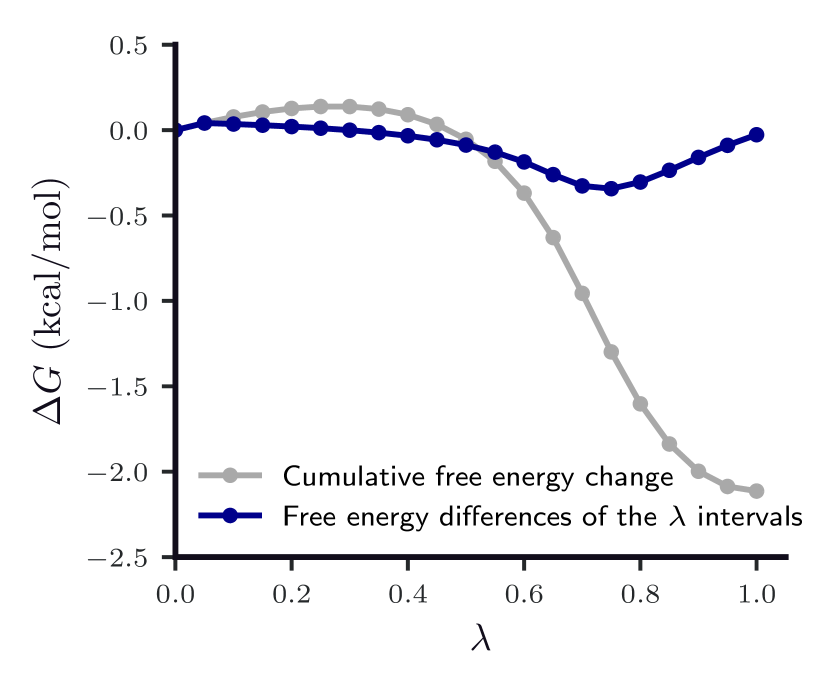
Figure 1: The free energy of solvating methane in water computed from alchemical simulations. The blue line indicates free energy differences between neighboring states, and the gray line is the cumulative free energy changes. The total free energy of solvation, i.e., the cumulative $\Delta G$ at $\lambda=1$, is estimated to be $2.13$ kcal/mol.

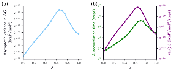
Figure 2: Analysis of the estimated error in the free energy of solvation for methane. (a) State contributions to the asymptotic variance of the free energy difference between the initial ($\lambda=0$) and final states ($\lambda=1$). (b) Breakdown of the error contributions into the integrated autocorrelation times and the variance of $\xi_{i}$. For ease of comparison, quantities are plotted on a logarithmic scale.

The total asymptotic standard deviation in the solvation free energy is estimated to be $0.0216\pm 0.0005$ kcal/mol using (52) with $\nabla\Phi$ given by (47). This is close to the standard deviation over all trials which is equal to $0.0225$ kcal/mol. The error contributions from all states are shown in Figure 2a. As the error contributions for different states can vary by more than two orders of magnitude, we have chosen to depict them on a logarithmic scale. Moreover, comparing with Figure 1 we see that the error contributions correlate with the magnitudes of the free energy differences between neighboring states. The fact that different states’ error contributions differ by orders of magnitudes suggests that the error in alchemical free energy simulations may be dominated by a few states. Authoritatively establishing this hypothesis would require further investigation over many alchemical simulations in a variety of settings. However, if similar phenomena do hold generically for other alchemical simulations, it may be possible to use error estimates to tune simulation parameters to achieve dramatic reductions in the error of MBAR estimates. Indeed, concurrent work that attempts to allocate sampling for alchemical simulations on the flyPredescu et al. (2021) suggests that better allocation of computational resources can substantially reduce the error in alchemical free energy simulations.

To further examine the source of the errors in our simulation, we attempt to disentangle the effect of the dynamics used to sample the state from effects inherent to the state definition. Recalling the definition of the integrated autocorrelation time in (11) and combining it with (52), we can further write the integrated autocovariance of each state as a product of the integrated autocorrelation time and a sampler-independent factor, namely, $\operatorname{var}\{\zeta_{i}\}$. In Figure 2b we plot both of the error components on a log scale: the logarithm of a state’s total contribution is a sum of the two curves. Our results show that capturing both the sampler-independent component of the error and the integrated autocorrelation time are important for estimating the total error contribution. Indeed, previous work has typically focused on optimizing the state parameters using solely thermodynamic properties; for instance, Shenfeld et al., 2009; Pham and Shirts, 2011 for instance, used information-geometric distances between states. However, our results suggest that to fully capture all sources of error, such approaches must also take into account kinetic effects from the specific choice of sampler used. This corrobates previous workPham and Shirts (2012) which has observed that the thermodynamical optimal choice of alchemical states may not be optimal in practice due to the resulting states having exceedingly large correlationtimes.

V.2 Umbrella Sampling Simulation of the Alanine Dipeptide

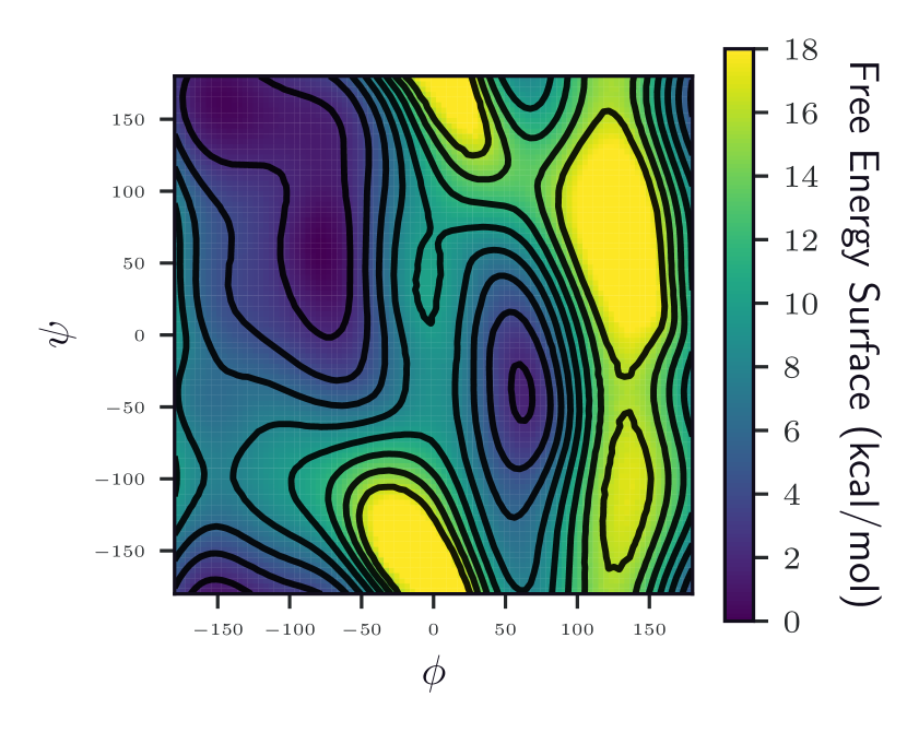
Figure 3: Free energy as a function of the $\phi$ and $\psi$ dihedral angles (measured in degrees) of the alanine dipeptide. The scale bar indicates free energy values in kcal/mol, and the contour spacing is $2$ kcal/mol.

We also applied the error estimator to a two-dimensional umbrella sampling simulation of the alanine dipeptide ($N$-acetyl-alanyl-$N^{\prime}$-methylamide) in vacuum. We performed 15 independent umbrella sampling calculations for the free energy as a function of the $\phi$ and $\psi$ dihedral angles. Simulations were run at 300 K using GROMACS version 2019.4Lindahl et al. (2019) with harmonic restraints applied to $\phi$ and $\psi$ using the PLUMED 2.5.3 software packageTribello et al. (2014). The molecule was represented by the AMBER force field with bonds to hydrogen atoms constrained by the LINCS algorithmHess et al. (1997). The force constant for the harmonic restraints was $0.0018$ kcal $\text{mol}^{-1}$ $\text{degree}^{-2}$, which corresponds to a Gaussian bias function with a standard deviation of $18\mathrm{°}$ in the absence of the molecular potential. We partitioned each dihedral angle into 30 intervals and placed the centers of the harmonic restraints at the centers of the cells of the resulting $30\times 30$ grid; the resulting grid ranged from $(-$$,-$$)$ to $($$,$$)$. Each state was sampled independently using the velocity Langevin dynamics integrator in GROMACS with a time step of 2 fs and a time constant of 0.1 ps. Each state was equilibrated for 40 ps and then sampled for 10 ms, with $\phi$ and $\psi$ values output every 0.4 ps.

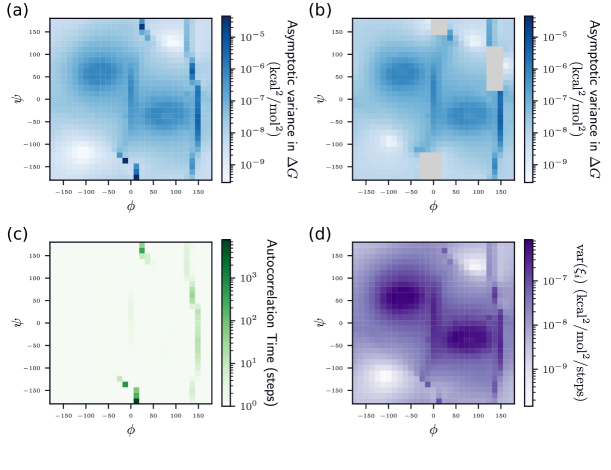
Figure 4: Analysis of the estimated error in the free energy difference between the C_7ax and C_7eq basins of the alanine dipeptide, shown on a logarithmic scale. (a) State contributions to the asymptotic variance of the free energy calculated using all states. (b) State contributions to the asymptotic variance of the free energy calculated using a set of states curated by analyzing the estimator for the asymptotic variance. States removed from the dataset are indicated in gray. (c) Integrated autocorrelation times of $\xi_{i}$ for the free energy estimate using every state. (d) Variance of $\xi_{i}$ for the free energy estimate using every state.

We used the MBAR equations to calculate the free energy as a function of $\phi$ and $\psi$ and, for each trial, the free energy difference between the C_7ax and C_7eq basins. We obtain the latter from the logarithm of the ratio of averages of two indicator functions. The C_7ax basin is defined as the region in the $\phi\psi$-space enclosed by a circle of radius $10\mathrm{°}$ centered at $($$,$$)$. The C_7eq basin is similarly defined by the circle of radius $10\mathrm{°}$ centered at $($$,$$)$.

In Table 1 we give our estimate of the error in the free energy difference evaluated as the asymptotic standard deviation (square root of the asymptotic error), as evaluated by (52), with $\nabla Phi$ given by (49). For comparison, we also give an estimate of the standard deviation calculated over 15 identical replicates. Our error estimate underestimates the true error by a factor of three, which we attribute to the difficulty in estimating the autocorrelation time accurately in the states. Comparing the plots of the integrated autocorrelation times in Figure 4c and the error contributions in Figure 4d to the free energy surface in Figure 3, we see that the error estimate is dominated by states in high-free energy regions that have long autocorrelation times. These states are located in regions where the alanine dipeptide is highly contorted, causing the free energy to increase sharply and complicating the task of sampling. For instance, states near free energy maxima can be bifurcated by a steep peak in the free energy. Sampling the state requires rare barrier-crossing events resulting in long autocorrelation times.

The fact that these states contribute considerably to our error estimate confirms the intuition that sampling unphysical regions can pollute free energy estimates. Indeed, this intuition has been the basis of a previous adaptive umbrella sampling algorithm Wojtas-Niziurski et al. (2013). To validate this idea, we removed several high-free energy states and recalculated both the estimate of the asymptotic error in the free energy difference as well as the standard deviation over the 15 replicates. We give the results in Table 1 and plot the resulting error contributions in Figure 4b with the removed states marked in gray. We see that the free energy estimate with high-free energy states filtered out has a lower error by a factor of three, despite the decrease in the amount of data. While we leave a systematic procedure for removing states for future work, our preliminary results, along with our earlier work on the Eigenvector Method for Umbrella Sampling and its application Thiede et al. (2016); Dinner et al. (2020); Antoszewski et al. (2020), demonstrate that our error estimates have the potential to improve the error of umbrella sampling and other multistate methods.

Table 1: Asymptotic standard deviation of the free energy between the C_7ax and C_7eq basins of the alanine dipeptide compared with the standard deviation over 15 independent simulations. The top row uses all states in the data set, while the bottom row uses insight from the error estimator to remove problematic states.

States Used	Estimated Asymptotic SD	SD over Replicates
	(kcal/mol)	(kcal/mol)
All	$0.0308\pm 0.0063$	$0.1125$
Curated	$0.0100\pm 0.0001$	$0.0377$

VI Conclusions

We derive a central limit theorem for estimates of both the normalization constants and function averages of the MBAR estimator. The central limit theorem allows us to devise a computational procedure for estimating the asymptotic error for arbitrary observables calculated through MBAR. In particular, it allows us to estimate the asymptotic error in free energy calculations. Notably, if states are sampled independently, the analytical expression of the total asymptotic error takes the form of a sum of contributions from all states. This enables us to trace how error in individual Markov chains contribute to the total error. Moreover, unlike previous error estimators, our approach explicitly accounts for the effects of correlation within each sampled trajectory.

We demonstrate the error estimator for an alchemical calculation of the solvation free energy of methane and a two-dimensional umbrella sampling calculation of the free energy of rearrangement of the alanine dipeptide. In both cases, the asymptotic error estimates agree reasonably well with the true error over all replicates. Moreover, for both our alchemical calculation and the umbrella sampling calculation we observe that the differences in the error contribution between states correlates strongly with the autocorrelation time of the associated states. For instance, for our umbrella sampling calculation, we observe that the error contributions are dominated by states in high-free energy regions in which dynamical variables decorrelate slowly. Upon the removal of those states, we see a significant error reduction. These results highlight the importance of error analysis that accounts for correlation in a sampled trajectory. We hope to investigate adaptive sampling strategies based on our error estimates in future work.

VII Acknowledgements

We wish to thank Jonathan Weare for advice and for pointing out a simplification in our error analyses, and Adam Antoszewski for helpful discussions. This work was supported by National Institutes of Health award R35 GM136381 and National Science Foundation awards DMS-2054306 and DMS-2012207. The Flatiron Institute is a division of the Simons Foundation.

Supplement for Understanding the Sources of Error in MBAR through Asymptotic Analysis

S1 Derivation of the Asymptotic Variance of MBAR

We prove that the MBAR estimator is asymptotically normal, and we give a convenient formula for the asymptotic variance. Our argument is based on the work of Geyer, 1994. Our contribution is to fill in details missing from Geyer’s manuscript and to correct errors. Most importantly, the formula for the asymptotic variance of observable averages $\left\langle g\right\rangle$ is not correct in the Geyer’s manuscript.

S1.1 The Maximum (Pseudo)likelihood Perspective

Following Geyer, 1994, we first introduce the MBAR estimate as the maximizer of a pseudolikelihood. We introduce the (absolute) free energy,

$$\eta_{j}=-\log(c_{j})$$

Define for any $y\in\mathbb{R}^{L}$,

$$\pi_{\mathrm{mix}}(x,y) =\sum_{k=1}^{L}\kappa_{k}q_{k}(x)\exp(y_{k}),\text{ and }$$ (S1)

$$p_{j}(x,y) =\frac{\kappa_{j}q_{j}(x)\exp(y_{j})}{\pi_{\mathrm{mix}}(x,y)}.$$ (S2)

We can then define the pseudolikelihood

$$l_{N}(y)=\frac{1}{N}\sum_{j=1}^{L}\sum_{t=1}^{N_{j}}\log p_{j}(X^{j}_{t},y)$$

based on a formal similarity with a logistic regression model. The MBAR estimating equation for $\bar{\eta}$ is equivalent with the first order optimality condition

$$\nabla l_{N}(\bar{\eta})=0$$ (S3)

for this pseudolikelihood. We refer to Gill, Vardi, and Wellner (1988); Vardi (1985); Geyer (1994); Kong et al. (2003) for more explanation of this perspective and for detailed derivations. Here, we merely observe that if samples are collected IID in each state then $l_{N}$ is the likelihood of the data given a particular value $y$ of the free energy. We note that this is not true for other sampling strategies where the samples are not IID, but one can still use (S3) to estimate $\eta$ even in that case. When written in maximum likelihood form and in terms of the variable $\eta$, the estimating equations have a very convenient structure. In particular, $l_{N}$ is concave and the Fisher information $\nabla^{2}l_{N}$ is a generator matrix. We will exploit aspects of this structure below.

Observe that $l_{N}$ is unchanged if one adds a constant to $y$, so (S3) determines $\bar{\eta}$ only up to an additive constant. Indeed, we chose to work with estimates of the relative free energies, which obey the constraint

$$\sum_{k=1}^{L}\bar{f}_{k}=0.$$ (S4)

With this particular constraint, $\bar{f}$ is not exactly an estimator of $\eta$, since we may have $\sum_{j=1}^{L}\eta_{j}\neq 0$. Instead, $\bar{f}$ converges to

$$f=\eta-\sum_{k=1}^{L}\eta_{k}.$$

We note that this arbitrary normalization of the free energies does not cause difficulties, since the MBAR formulas for observable averages are unchanged if one adds a constant to $\bar{f}$ and only free energy differences are important for most applications.

When the constraint (S4) is imposed, one can show that if the matrix

$$\bar{M}_{ij}=\frac{1}{N_{j}}\sum_{t=1}^{N_{j}}q_{i}(X^{j}_{t})$$

is irreducible, then (S3) determines a unique $\bar{f}$, cf.Theorem 1 in Ref. Geyer, 1994 and Theorem 1.1 in Ref. Gill, Vardi, and Wellner, 1988. Moreover, if $M_{ij}=\langle q_{i}\rangle_{j}$ is irreducible, then (a) with probability one $\bar{M}$ is irreducible for sufficiently large $N$ (cf.Theorem 1 in Ref. Geyer, 1994 or Proposition 1.1 in Ref. Gill, Vardi, and Wellner, 1988) and (b) $\bar{f}\xrightarrow{as}f$ (cf.Theorem 1 in Ref. Geyer, 1994). When $M_{ij}=\langle q_{i}\rangle_{j}$ is irreducible, we say that the densities $q_{1},\dots,q_{L}$ are inseparable. We will assume inseparability throughout the remainder of this work:

Assumption S1.1.

We assume that the densities $q_{1},\dots,q_{L}$ are inseparable, i.e.the matrix $M_{ij}=\langle q_{i}\rangle_{j}$ is irreducible.

Once estimates of the free energies $\bar{f}$ have been constructed, averages of observables are estimated in terms of quantities of the form

$$\bar{\omega}_{i}(\bar{f})=\sum_{k=1}^{L}\kappa_{k}\frac{1}{N_{k}}\sum_{t=1}^{N_{k}}\frac{w_{i}(X^{k}_{t})}{\pi_{\mathrm{mix}}(X^{k}_{t},\bar{f})}$$ (S5)

for some functions $w_{1},\dots,w_{M}$, as explained in the text.

S1.2 Outline of Proof of Asymptotic Normality

We will prove asymptotic normality of $(\bar{f},\bar{\omega}(\bar{f}))$. To do so, it is expedient to define the function $\bar{F}:\mathbb{R}^{L}\times\mathbb{R}^{M}\rightarrow\mathbb{R}^{L}\times\mathbb{R}^{M}$ by

$$\bar{F}(y,z)=(\nabla l_{N}(y),z-\bar{\omega}(y)),$$

where $\bar{\omega}(y)$ is defined by (S5) but with $y$ in place of $\bar{f}$. Under Assumption S1.1, $(\bar{f},\bar{\omega}(\bar{f}))$ is the unique root of $\bar{F}$ for $N$ sufficiently large. We will proceed as follows: First, we show that for any fixed $(y,z)\in\mathbb{R}^{L}\times\mathbb{R}^{M}$, a LLN and CLT hold for $\bar{F}(y,z)$, so

$$\bar{F}(y,z) \xrightarrow{as}F(y,z)$$

and

$$\sqrt{N}(\bar{F}(y,z)-F(y,z)) \xrightarrow{d}N(0,A(y,z))$$

for some limiting value $F(y,z)$ and covariance matrix $A(y,z)$. Second, we compute a Taylor expansion of roughly the form

$$\bar{F}(\bar{f},\bar{\omega}(\bar{f}))-\bar{F}(f,\omega)=-\bar{F}(f,\omega)=\bar{F}^{\prime}(f,\omega)((\bar{f},\bar{\omega}(\bar{f}))-(f,\omega))+\text{ higher order terms},$$

where $\omega$ is the limiting value of $\bar{\omega}(f)$ defined in (S11). Third, we derive a matrix $\bar{\Gamma}$ that acts as a generalized inverse for $\bar{F}^{\prime}$ in the Taylor expansion, which gives

$$-\bar{\Gamma}\bar{F}(f,\omega)=(\bar{f},\bar{\omega}(\bar{f}))-(f,\omega)+\text{ higher order terms}.$$

We show that $\bar{\Gamma}$ converges almost surely to a limit $\Gamma$, and we give an explicit formula for $\Gamma$. Finally, we conclude by Slutsky’s theorem and the CLT for $\bar{F}(y,z)$ that

$$\sqrt{N}((\bar{f},\bar{\omega}(\bar{f}))-(f,\omega))=-\bar{\Gamma}\sqrt{N}(\bar{F}(f,\omega)-F(f,\omega))+\text{higher order terms}\xrightarrow{d}N(0,\Gamma A(f,\omega)\Gamma^{t}).$$

S1.3 Derivatives of $l_{N}$ and $\bar{\omega}$

The proof outlined above requires the Taylor expansion of $\bar{F}$ at $(f,\omega)$. We begin by computing the derivatives of $l_{N}$ and also some upper bounds on derivatives that we will use to estimate higher order terms in our expansion. We observe that

$$\frac{\partial p_{j}(x,y)}{\partial y_{l}} =\frac{\partial}{\partial y_{l}}\frac{\kappa_{j}q_{j}(x)\exp(y_{j})}{\sum_{k=1}^{L}\kappa_{k}q_{k}(x)\exp(y_{k})}$$

$$=p_{j}(x,y)(\delta_{lj}-p_{l}(x,y)).$$

Therefore,

$$\frac{\partial l_{N}}{\partial y_{l}}(y) =\kappa_{l}-\frac{1}{N}\sum_{k=1}^{L}\sum_{t=1}^{N_{k}}p_{l}(X^{k}_{t},y),$$

$$\frac{\partial l_{N}}{\partial y_{l}\partial y_{m}}(y) =\begin{cases}-\frac{1}{N}\sum_{k=1}^{L}\sum_{t=1}^{N_{k}}p_{l}(X^{k}_{t},y)(1-p_{l}(X^{k}_{t},y))&\text{ if }l=m\\ \frac{1}{N}\sum_{k=1}^{L}\sum_{t=1}^{N_{k}}p_{l}(X^{k}_{t},y)p_{m}(X^{k}_{t},y)&\text{ if }l\neq m.\end{cases}$$

Moreover, one sees immediately from the analogous formula for third derivatives (and using $0\leq p_{l}(x,y)\leq 1$) that

$$\left\lvert\frac{\partial l_{N}}{\partial y_{l}\partial y_{m}\partial y_{p}}(y)\right\rvert\leq 2.$$ (S6)

This will allow us to control the error terms of the Taylor expansion.

We also require derivatives of the $\bar{\omega}_{i}$’s. Define for any $y\in\mathbb{R}^{L}$,

$$\bar{\omega}_{i}(y)=\frac{1}{N}\sum_{k=1}^{L}\sum_{t=1}^{N_{K}}\frac{w_{i}(X^{k}_{t})}{\pi_{\mathrm{mix}}(X^{k}_{t},y)}.$$

We have

$$\frac{\partial\bar{\omega}_{i}}{\partial y_{l}}(y) =-\frac{1}{N}\sum_{k=1}^{L}\sum_{t=1}^{N_{K}}\frac{w_{i}(X^{k}_{t})}{\pi_{\mathrm{mix}}(X^{k}_{t},y)}p_{l}(X^{k}_{t},y),$$

$$\frac{\partial\bar{\omega}_{i}}{\partial y_{l}y_{m}}(y) =\frac{1}{N}\sum_{k=1}^{L}\sum_{t=1}^{N_{K}}\frac{w_{i}(X^{k}_{t})}{\pi_{\mathrm{mix}}(X^{k}_{t},y)}(p_{l}(X^{k}_{t},y)p_{m}(X^{k}_{t},y)-p_{l}(X^{k}_{t},y)(\delta_{lm}-p_{m}(X^{k}_{t},y))$$

$$=\frac{1}{N}\sum_{k=1}^{L}\sum_{t=1}^{N_{K}}\frac{w_{i}(X^{k}_{t})}{\pi_{\mathrm{mix}}(X^{k}_{t},y)}2p_{l}(X^{k}_{t},y)(p_{m}(X^{k}_{t},y)-\delta_{lm}).$$

Note that the second order partial derivatives are bounded independently of $N$:

$$\left\lvert\frac{\partial\bar{\omega}_{i}}{\partial y_{l}\partial y_{m}}(y)\right\rvert\leq 2\max_{x}\left\lvert\frac{w_{i}(x)}{\pi_{\mathrm{mix}}(x,y)}\right\rvert.$$ (S7)

To control the error terms in our Taylor approximation, we will assume that the right hand side of (S7) is bounded uniformly in $x$ for fixed $y$.

Assumption S1.2.

For any $y\in\mathbb{R}^{L}$, there exists $C(y)>0$ so that

$$\max_{x}\left\lvert\frac{w_{i}(x)}{\pi_{\mathrm{mix}}(x,y)}\right\rvert\leq C(y)$$

for all $i=1,\dots,M$.

We expect Assumption S1.2 to hold in practice for both umbrella sampling and alchemical calculations. First, consider umbrella sampling, where $w_{i}=g_{i}q$ for some observables $g_{i}$ and $q_{k}=\psi_{k}q$ for some biasing functions $\psi_{k}$. Typically, the observables are bounded, so for some $D>0$,

$$\lvert g_{i}(x)\rvert\leq D$$ (S8)

for all $x$ and $i=1,\dots,M$. In addition, we may assume that for some $E>0$,

$$\left\lvert\frac{1}{\sum_{k}\psi_{k}(x)}\right\rvert\leq E$$ (S9)

for all $x$. We note that (S9) holds if the biasing functions $\psi_{i}$ are a partition of unity and also in the other cases considered in Thiede et al., 2016 and Dinner et al. (2020). If (S8) and (S9) hold, then Assumption S1.2 holds with

$$C(y)=\frac{DE}{\min_{k}\exp(y_{k})}.$$

In the alchemical case, if we are only interested in a free energy difference, then Assumption S1.2 is irrelevant since we need only estimate $z_{1}/z_{L}$. If we also want the averages of an observable $g$ over the densities $q_{i}$, then we choose $w_{i}=gq_{i}$ and Assumption S1.2 holds with

$$C(y)=\frac{\max_{x}\lvert g(x)\rvert}{\min_{k}\exp(y_{k})},$$

assuming that $g$ is bounded.

S1.4 Ergodicity and the Central Limit Theorem for $\bar{F}$

Observe that for any fixed $y\in\mathbb{R}^{L}$, $l_{N}(y)$, $\bar{\omega}(y)$, and their derivatives are all linear combinations of ergodic averages of fixed functions over the processes $X^{i}_{t}$. We assume that these ergodic averages converge as $N\rightarrow\infty$.

Assumption S1.3.

For any bounded measurable $g:\mathbb{R}^{n}\rightarrow\mathbb{R}^{m}$, we have

$$\frac{1}{N}\sum_{j=1}^{L}\sum_{t=1}^{N_{j}}g(X^{j}_{t})\xrightarrow{as}\mathbf{E}[g(X)],$$

where $X$ is a random variable with density proportional to $\pi_{\mathrm{mix}}(\cdot,f)$.

If $\kappa_{i}=N_{i}/N$ is independent of $N$, Assumption S1.3 holds as long as each of the chains $X^{j}_{t}$ is ergodic. (In fact, it is enough that $\limsup_{N\rightarrow\infty}\kappa_{i}>0$ for all $i$. We will not discuss this more general possibility, but see the assumptions made in Ref. Geyer (1994) and Ref. Gill, Vardi, and Wellner (1988).)

Observe that for any fixed $y\in\mathbb{R}^{L}$, $p_{l}(x,y)$ is a bounded and measurable function of $x$. Therefore, by Assumption S1.3 and the formulas derived in Section S1.3, for any fixed $y\in\mathbb{R}^{L}$,

$$\begin{split}\frac{\partial l_{N}}{\partial f_{l}}(y)\xrightarrow{as}G_{l}(y)&=\kappa_{l}-\mathbf{E}[p_{l}(X,y)],\\ \frac{\partial l_{N}}{\partial f_{l}\partial f_{m}}(y)\xrightarrow{as}H_{lm}(y)&=\begin{cases}-\mathbf{E}[p_{l}(X,y)(1-p_{l}(X,y))]&\text{ if }l=m\\ \mathbf{E}[p_{l}(X,y)p_{m}(X,y)]&\text{ if }l\neq m,\end{cases}\end{split}$$ (S10)

where $X$ is a random variable with density proportional to $\pi_{\mathrm{mix}}(\cdot,f)$. Similarly,

$$\begin{split}\bar{\omega}_{i}(y)\xrightarrow{a.s.}\omega_{i}(y)&=\mathbf{E}\left[\frac{w_{i}(X)}{\pi_{\mathrm{mix}}(X,y)}\right],\\ \frac{\partial\bar{\omega}_{i}}{\partial f_{l}}(y)\xrightarrow{a.s.}dw_{il}(y)&=\mathbf{E}\left[\frac{w_{i}(X)}{\pi_{\mathrm{mix}}(X,y)}p_{l}(X,y)\right],\end{split}$$ (S11)

where again $X$ is a random variable with density proportional to $\pi_{\mathrm{mix}}(\cdot,f)$. It follows that

$$\bar{F}(y,z)\xrightarrow{as}F(y,z)=(G(y),z-\omega(y)).$$

We also assume that a central limit theorem holds.

Assumption S1.4.

For any fixed $(y,z)\in\mathbb{R}^{L}\times\mathbb{R}^{M}$,

$$\sqrt{N}(\bar{F}(y,z)-F(y,z)) \xrightarrow{d}N(0,A(y,z))$$

for some covariance matrix $A(y,z)\in\mathbb{R}^{(L+M)\times(L+M)}$.

Assumption S1.4 is a consequence of assumption (39) in the main text. When assumption (39) holds, $A(f,\omega)$ is the same as the matrix $A$ defined in the main text in the statement of Theorem IV.1.

S1.5 The Linearization of $\bar{F}$ and its Generalized Inverse

We will transform the central limit theorem for $\bar{F}$ to a central limit theorem for $(\bar{f},\bar{\omega}(\bar{f}))$ by applying a generalized inverse of the linearization of $\bar{F}$ at $(f,\omega)$ . The basic idea is very similar to the delta method. In this subsection, we derive the appropriate linearization and generalized inverse.

Define

$$\bar{v}=(\bar{f},\bar{\omega}(\bar{f}))\text{ and }v=(f,\omega).$$

We have

$$\bar{F}(\bar{v})-\bar{F}(v)=-\bar{F}(v)=-(\bar{F}(v)-F(v))=\bar{B}(\bar{v}-v),$$

where

$$\bar{B}=\int_{s=0}^{1}\bar{F}^{\prime}(s\bar{v}+(1-s)v)\,ds.$$

(Here, we use that $\bar{F}(\bar{v})=F(v)=0$.) We will demonstrate the existence of a generalized inverse $\bar{\Gamma}$ of $\bar{B}$ so that

$$\bar{\Gamma}\bar{B}(\bar{v}-v)=\bar{v}-v,$$

and we will show that $\bar{\Gamma}$ converges almost surely to a certain matrix $\Gamma$.

To devise the right $\bar{\Gamma}$, we first observe that

$$\bar{F}^{\prime}(y,z)=\begin{pmatrix}\nabla^{2}l_{N}(y)&0\\ -\frac{\partial\bar{\omega}}{\partial y}(y,z)&I\end{pmatrix}.$$

Here, $\nabla^{2}l_{N}(y)\in\mathbb{R}^{L\times L}$ denotes the Hessian matrix of $l_{N}$, $\frac{\partial\bar{\omega}}{\partial y}\in\mathbb{R}^{M\times L}$ with $\left(\frac{\partial\bar{\omega}}{\partial y}\right)_{ij}=\frac{\partial\bar{\omega}_{i-L}}{\partial y_{j}}$, and $I\in\mathbb{R}^{M\times M}$ is the identity matrix.

We observe that for any value of $x$,

$$-\nabla^{2}l_{N}(y)=I-\bar{P}(y),$$

where $\bar{P}$ is the symmetric, stochastic matrix

$$\bar{P}_{lm}(y)=\begin{cases}1-\frac{1}{N}\sum_{k=1}^{L}\sum_{t=1}^{N_{k}}p_{l}(X^{k}_{t},y)(1-p_{l}(X^{k}_{t},y))&\text{ if }l=m\\ \frac{1}{N}\sum_{k=1}^{L}\sum_{t=1}^{N_{k}}p_{l}(X^{k}_{t},y)p_{m}(X^{k}_{t},y)&\text{ if }l\neq m.\end{cases}$$

That is, $-\nabla^{2}l_{N}(y)$ is a generator matrix. To see that $\bar{P}(y)$ is indeed stochastic, first observe that

$$\bar{P}_{ii}(y)\geq\frac{3}{4},$$

since we have $p_{l}(x,y)(1-p_{l}(x,y))\leq\frac{1}{4}$ for all $x,y,l$, and so the diagonal entries are positive. The off-diagonal entries are nonnegative since $p_{l}(x,y)\geq 0$ for all $x,y,l$, and the rows sum to one since $\sum_{l}p_{l}(x,y)=1$ for all $x,y$. When the $q_{i}$’s are inseparable, under Assumption S1.1, $\bar{P}(x)$ is irreducible for sufficiently large $N$. Moreover, $\bar{P}(y)$ is aperiodic since its diagonal is positive.

Now let

$$\bar{H}:=\int_{s=0}^{1}\nabla^{2}l_{N}(s\bar{f}+(1-s)f)\,ds=\bar{Q}-I,$$

where

$$\bar{Q}:=\int_{s=0}^{1}\bar{P}(s\bar{f}+(1-s)f)\,ds.$$

Note that $\bar{Q}$ is stochastic, and that it inherits symmetry, irreducibility, and aperiodicity from $\bar{P}$. It follows from symmetry and irreducibility that $L^{-1}\mathds{1}$ is the unique invariant distribution of $\bar{Q}$, and therefore by Theorem 5.5 in Meyer, 1975 the group inverse $\bar{H}^{\#}$ of $\bar{H}$ exists and is given by

$$\bar{H}^{\#}=L^{-2}\mathds{1}\mathds{1}^{t}+(\bar{H}-L^{-2}\mathds{1}\mathds{1}^{t})^{-1}.$$ (S12)

The group inverse is a particular type of generalized inverse similar to the Moore-Penrose inverse. (In fact, the group inverse of $H$ is the same as its Moore-Penrose inverse. We prefer to call it the group inverse since we will use the results of Meyer Meyer (1975) on group inverses of generator matrices.) The group inverse is characterized by the properties

$$\bar{H}\bar{H}^{.}\#=\bar{H}^{\#}\bar{H},\text{ }\bar{H}^{\#}\bar{H}\bar{H}^{\#}=\bar{H}^{\#},\text{ and }\bar{H}\bar{H}^{\#}\bar{H}=\bar{H}.$$

We refer to Meyer, 1975; Golub and Meyer, 1986 for details. For future reference, we also note that by Theorem 2.2 in Meyer, 1975, we have

$$\bar{H}^{\#}\bar{H}=I-L^{-2}\mathds{1}\mathds{1}^{t}.$$ (S13)

We will use $\bar{H}^{\#}$ as a building block of our generalized inverse $\bar{\Gamma}$. We have

$$\bar{B}=\int_{s=0}^{1}\bar{F}^{\prime}(s\bar{v}+(1-s)v)\,ds=\begin{pmatrix}\bar{H}&0\\ \overline{dw}&I\end{pmatrix},$$

where

$$\overline{dw}:=\int_{s=0}^{1}\frac{\partial\omega}{\partial y}(s\bar{v}+(1-s)v)\,ds.$$

We define

$$\bar{\Gamma}=\begin{pmatrix}\bar{H}^{\#}&0\\ -\overline{dw}\bar{H}^{\#}&I\end{pmatrix}.$$

Observe that by (S13),

$$\bar{\Gamma}\bar{B}=\begin{pmatrix}\bar{H}^{\#}&0\\ -\overline{dw}\bar{H}^{\#}&I\end{pmatrix}\begin{pmatrix}\bar{H}&0\\ \overline{dw}&I\end{pmatrix}=\begin{pmatrix}I-L^{-2}\mathds{1}\mathds{1}^{t}&0\\ \overline{dw}(I-L^{-2}\mathds{1}\mathds{1}^{t})&I\end{pmatrix}.$$

Therefore, since

$$\mathds{1}^{t}\bar{f}=\mathds{1}^{t}f=0$$

by the constraint (S4), we have

$$\bar{\Gamma}\bar{B}(\bar{v}-v)=\bar{v}-v.$$ (S14)

Equation (S14) is one of the desired properties of $\bar{\Gamma}$. We will now show in addition that

$$\bar{\Gamma}\xrightarrow{as}\Gamma:=\begin{pmatrix}H(f)^{\#}&0\\ -dw(f,w)H(f)^{\#}&I\end{pmatrix}.$$ (S15)

First, we show that

$$\bar{H}\xrightarrow{as}H(f).$$ (S16)

We have

$$\bar{H}_{lm} =h_{1}+h_{2},$$

where

$$h_{1} :=\int_{s=0}^{1}\frac{\partial l_{N}}{\partial y_{l}\partial y_{m}}(s\bar{f}+(1-s)f)-\frac{\partial l_{N}}{\partial y_{l}\partial y_{m}}(f)\,ds,\text{ and }$$

$$h_{2} :=\frac{\partial l_{N}}{\partial y_{l}\partial y_{m}}(f).$$

Using the uniform bounds on third derivatives of the likelihood (S6),

$$\lvert h_{1}\rvert \leq 2L\max_{k}\lvert\bar{f}_{k}-f_{k}\rvert,$$

and therefore

$$h_{1}\xrightarrow{as}0,$$

since as discussed above we have $\bar{f}\xrightarrow{as}f$ by the results of Geyer Geyer (1994). By (S10),

$$h_{2}\xrightarrow{as}H(f).$$

Thus, (S16) holds. A similar argument using (S7) and (S11) shows that

$$\bar{d}w\xrightarrow{as}dw(f,\omega).$$

To complete the proof that $\bar{\Gamma}\xrightarrow{as}\Gamma$, consider formula (S12) for $\bar{H}^{\#}$. The right hand side

$$L^{-2}\mathds{1}\mathds{1}^{t}+(\bar{H}-L^{-2}\mathds{1}\mathds{1}^{t})^{-1}$$

of (S12) is continuous as a function of $\bar{H}$ over an open neighborhood of any $\bar{H}$ so that the inverse exists, since the matrix inverse is a continuous function on a neighborhood of any nonsingular matrix. In particular, it is continuous at $H(f)$, since $H(f)$ is stochastic, symmetric, irreducible, and aperiodic by the same argument that shows that $\bar{H}$ has these properties. It follows that

$$\bar{H}^{\#}\xrightarrow{as}L^{-2}\mathds{1}\mathds{1}^{t}+(H(f)-L^{-2}\mathds{1}\mathds{1}^{t})^{-1}=H(f)^{\#},$$

hence

$$\bar{\Gamma}\xrightarrow{as}\Gamma.$$

Combining the results of the previous sections yields the following theorem.

Theorem S1.5.

Under Assumptions S1.1, S1.2, S1.3, and S1.4, we have

$$\sqrt{N}(\bar{v}-v)\xrightarrow{d}N(0,\Gamma A(v)\Gamma^{t}).$$ (S17)

Proof.

By the results of Section S1.5,

$$-\bar{\Gamma}\sqrt{N}(\bar{F}(v)-F(v))=\sqrt{N}(\bar{v}-v),$$

and the result follows from Slutsky’s theorem and the CLT for $\bar{F}(v)$. ∎

S1.6 A Simple Expression for $\Gamma$

The matrix $\Gamma$ can be further simplified by observing that

$$H_{lm}(f)= -\delta_{lm}\mathbf{E}[p_{l}(X,f)]+\mathbf{E}[p_{l}(X,f)p_{m}(X,f)]$$

$$= -\delta_{lm}\sum_{i=1}^{L}\exp(f_{i})\int p_{l}(x,f)q_{i}(x)dx+\sum_{i=1}^{L}\exp(f_{i})\int p_{l}(x,f)p_{m}(x,f)q_{i}(x)dx$$

$$= -\delta_{lm}\sum_{i=1}^{L}\exp(f_{i})\int\frac{q_{l}(x)\exp(f_{l})}{\sum_{j}q_{j}(x)\exp(f_{j})}q_{i}(x)dx+\sum_{i=1}^{L}\exp(f_{i})\int\frac{q_{l}(x)\exp(f_{l})}{\left(\sum_{k}q_{k}(x)\exp(f_{k})\right)}p_{m}(x,f)q_{i}(x)dx$$

$$= -\int\left(\frac{\delta_{lm}q_{l}(x)\exp(f_{l})}{\sum_{j}q_{j}(x)\exp(f_{j})}-\frac{q_{l}(x)\exp(f_{l})}{\sum_{k}q_{k}(x)\exp(f_{k})}p_{m}(x,f)\right)\left(\sum_{i=1}^{L}q_{i}(x)\exp(f_{i})\right)dx$$

$$= -\int\left(\delta_{lm}q_{l}(x)\exp(f_{l})-p_{m}(x,f)q_{l}(x)\exp(f_{l})\right)dx$$

$$= -\delta_{lm}\int q_{l}(x)\exp(f_{l})dx+\int p_{m}(x,f)q_{l}(x)\exp(f_{l})dx$$

$$= -\delta_{lm}\kappa_{l}+\frac{\kappa_{l}}{c_{l}}\int p_{m}(x,f)q_{l}(x)dx,$$

where the final line follows from the fact that $q_{l}(x)/c_{l}$ is a probability density and consequently integrates to one. Similarly, we have that

$$dw_{il}(v) =\sum_{i=1}^{L}\exp(f_{i})\int\frac{w_{i}(X)p_{l}(X,f)}{\pi_{\mathrm{mix}}(X,f)}q_{i}(x)dx$$

$$=\int\left(\frac{w_{i}(X)}{\sum_{j=1}^{L}q_{j}(x)\exp(f_{j})}\right)\left(\frac{q_{l}(x)\exp(f_{l})}{\sum_{j=1}^{L}q_{j}(x)\exp(f_{j})}\right)\left(\sum_{i=1}^{L}\exp(f_{i})q_{i}(x)\right)dx$$

$$=\int\left(\frac{w_{i}(X)}{\sum_{j=1}^{L}q_{j}(x)\exp(f_{j})}\right)q_{l}(x)\exp(f_{l})dx$$

$$=\int\left(\frac{w_{i}(X)}{\sum_{j=1}^{L}q_{j}(x)\exp(f_{j})}\right)q_{l}(x)\exp(f_{l})dx$$

S2 Data-driven Estimates of the Asymptotic Variance

Here, we cover in more detail the derivation of our expressions for the asymptotic variance of MBAR estimates from trajectory autocorrelations. We consider two cases: the case where each state is sampled independently of all the other states with its own Markov chain (as in many Umbrella sampling and Alchemical Simulation calculations), and the case where all states are sampled together using a single joint Markov chain (as in Parallel Tempering and Hamiltonian Replica Exchange).

S2.1 Independent Sampling of States

As observed in the main text, if states are sampled independently then $\Xi^{lm}$ is nonzero if and only if $l=m$. We can therefore write

$$\big{(}\nabla\Phi^{T}(v) {\Gamma}A\Gamma^{T}\nabla\Phi(v)\big{)}_{im}=\sum_{j=1}^{L+M}\sum_{k}^{L+M}\sum_{l=1}^{L}(\nabla\Phi^{T}{\Gamma}(v))_{ij}\kappa_{l}\Xi_{jk}^{ll}(\Gamma^{T}\nabla\Phi(v))_{km}$$

$$= \sum_{j=1}^{L+M}\sum_{k}^{L+M}\sum_{l=1}^{L}(\nabla\Phi^{T}{\Gamma}(v))_{ij}\kappa_{l}\bigg{(}\operatorname{cov}\left\{\xi_{j}(X_{t}^{l},v),\xi_{k}(X_{t}^{l},v)\right\}+2\sum_{\tau=1}^{\infty}\operatorname{cov}\left\{\xi_{j}(X_{t}^{l},v),\xi_{k}(X_{t+\tau}^{l},v)\right\}\bigg{)}(\Gamma^{T}\nabla\Phi(v))_{km}$$

$$= \sum_{l=1}^{L}\kappa_{l}\bigg{(}\operatorname{cov}\left\{\sum_{j=1}^{L+M}(\nabla\Phi^{T}{\Gamma}(v))_{ij}\xi_{j}(X_{t}^{l},v),\sum_{k}^{L+M}(\Gamma^{T}\nabla\Phi(v))_{km}\xi_{k}(X_{t}^{l},v)\right\}$$

$$\qquad\quad+2\sum_{\tau=1}^{\infty}\operatorname{cov}\left\{\sum_{j=1}^{L+M}(\nabla\Phi^{T}{\Gamma}(v))_{ij}\xi_{j}(X_{t}^{l},v),\sum_{k}^{L+M}(\Gamma^{T}\nabla\Phi(v))_{km}\xi_{k}(X_{t+\tau}^{l},v)\right\}\bigg{)}$$

$$= \sum_{l=1}^{L}\bigg{(}\operatorname{cov}\left\{\chi_{i}(X_{t}^{l}),\chi_{m}(X_{t}^{l})\right\}+2\sum_{\tau=1}^{\infty}\operatorname{cov}\left\{\chi_{i}(X_{t}^{l}),\chi_{m}(X_{t+\tau}^{l})\right\}\bigg{)}$$ (S18)

which recovers equation 52 in the main text.

S2.2 Joint Sampling of States

Alternatively, we can consider the case where, for a given $t$, the $X_{i}^{t}$’s are collected jointly for all $i$ from a single Markov chain. By definition we then have the same number of points in every state and $\kappa_{i}=(1/L)$ for all $i$. We then write

$$\big{(}\nabla\Phi^{T}(v) {\Gamma}A\Gamma^{T}\nabla\Phi(v)\big{)}_{in}=\sum_{j=1}^{L+M}\sum_{k}^{L+M}\sum_{l=1}^{L}\sum_{m=1}^{L}(\nabla\Phi^{T}{\Gamma}(v))_{ij}(1/L)\Xi_{jk}^{lm}(\Gamma^{T}\nabla\Phi(v))_{kn}$$

$$= \frac{1}{L}\sum_{j=1}^{L+M}\sum_{k}^{L+M}\sum_{l=1}^{L}\sum_{m=1}^{L}(\nabla\Phi^{T}{\Gamma}(v))_{ij}\kappa_{l}\bigg{(}\operatorname{cov}\left\{\xi_{j}(X_{t}^{l},v),\xi_{k}(X_{t}^{m},v)\right\}+$$

$$\qquad\quad+2\sum_{\tau=1}^{\infty}\operatorname{cov}\left\{\xi_{j}(X_{t}^{l},v),\xi_{k}(X_{t+\tau}^{m},v)\right\}\bigg{)}(\Gamma^{T}\nabla\Phi(v))_{kn}$$

$$= (1/L)\bigg{(}\operatorname{cov}\left\{\sum_{l=1}^{L}\sum_{j=1}^{L+M}(\nabla\Phi^{T}{\Gamma}(v))_{ij}\xi_{j}(X_{t}^{l},v),\sum_{m=1}^{L}\sum_{k}^{L+M}(\Gamma^{T}\nabla\Phi(v))_{km}\xi_{k}(X_{t}^{m},v)\right\}$$

$$\qquad\quad+2\sum_{\tau=1}^{\infty}\operatorname{cov}\left\{\sum_{l=1}^{L}\sum_{j=1}^{L+M}(\nabla\Phi^{T}{\Gamma}(v))_{ij}\xi_{j}(X_{t}^{l},v),\sum_{m=1}^{L}\sum_{k}^{L+M}(\Gamma^{T}\nabla\Phi(v))_{kn}\xi_{k}(X_{t+\tau}^{m},v)\right\}\bigg{)}$$

$$= \bigg{(}\operatorname{cov}\left\{\sum_{l=1}^{L}\chi_{i}(X_{t}^{l})),\sum_{m=1}^{L}\chi_{n}(X_{t}^{m})\right\}+2\sum_{\tau=1}^{\infty}\operatorname{cov}\left\{\sum_{l=1}^{L}\chi_{i}(X_{t}^{l}),\sum_{m=1}^{L}\chi_{n}(X_{t+\tau}^{m})\right\}\bigg{)}$$ (S19)

References

- Chipot and Pohorille (2007) C. Chipot and A. Pohorille, “Free energy calculations,” Springer Series in Chemical Physics 86, 159–184 (2007).
- Lelièvre, Rousset, and Stoltz (2010) T. Lelièvre, M. Rousset, and G. Stoltz, Free energy computations (Imperial College Press, London, 2010).
- Dinner et al. (2020) A. R. Dinner, E. H. Thiede, B. V. Koten, and J. Weare, “Stratification as a general variance reduction method for Markov chain Monte Carlo,” SIAM/ASA Journal on Uncertainty Quantification 8, 1139–1188 (2020).
- Torrie and Valleau (1977) G. M. Torrie and J. P. Valleau, “Nonphysical sampling distributions in Monte Carlo free-energy estimation: Umbrella sampling,” Journal of Computational Physics 23, 187 (1977).
- Pangali, Rao, and Berne (1979) C. Pangali, M. Rao, and B. J. Berne, “A Monte Carlo simulation of the hydrophobic interaction,” The Journal of Chemical Physics 71, 2975–2981 (1979), https://aip.scitation.org/doi/pdf/10.1063/1.438701 .
- Swendsen and Wang (1986) R. H. Swendsen and J.-S. Wang, “Replica Monte Carlo simulation of spin-glasses,” Physical review letters 57, 2607 (1986).
- Geyer (1991) C. J. Geyer, “Markov chain Monte Carlo maximum likelihood,” in Computing Science and Statistics: Proceedings of the rd Symposium on the Interface (American Statistical Association, 1991).
- Tembre and Mc Cammon (1984) B. L. Tembre and J. A. Mc Cammon, “Ligand-receptor interactions,” Computers & Chemistry 8, 281–283 (1984).
- Frenkel and Smit (2002) D. Frenkel and B. Smit, Understanding molecular simulation from algorithms to applications, Computational Science (Academic Press, San Diego, 2002) p. 638.
- Chodera et al. (2011) J. D. Chodera, D. L. Mobley, M. R. Shirts, R. W. Dixon, K. Branson, and V. S. Pande, “Alchemical free energy methods for drug discovery: progress and challenges,” Current Opinion in Structural Biology 21, 150–160 (2011).
- Shirts and Chodera (2008) M. R. Shirts and J. D. Chodera, “Statistically optimal analysis of samples from multiple equilibrium states,” The Journal of Chemical Physics 129, 124105 (2008).
- Vardi (1985) Y. Vardi, “Empirical distributions in selection bias models,” The Annals of Statistics 13, 178–203 (1985).
- Kong et al. (2003) A. Kong, P. McCullagh, X.-L. Meng, D. Nicolae, and Z. Tan, “A theory of statistical models for Monte Carlo integration,” Journal of the Royal Statistical Society: Series B (Statistical Methodology) 65, 585–604 (2003).
- Thiede et al. (2016) E. H. Thiede, B. Van Koten, J. Weare, and A. R. Dinner, “Eigenvector method for umbrella sampling enables error analysis,” The Journal of Chemical Physics 145, 084115 (2016).
- Chan (1993) K. Chan, “On the central limit theorem for an ergodic Markov chain,” Stochastic processes and their applications 47, 113–117 (1993).
- Tierney (1994) L. Tierney, “Markov chains for exploring posterior distributions,” The Annals of Statistics 22, 1701–1728 (1994).
- Geyer and Chan (1994) C. Geyer and K. Chan, “Discussion of the paper by Tierney,” Annals of Statistics 22, 1747–1758 (1994).
- Jones (2004) G. L. Jones, “On the Markov chain central limit theorem,” Probability Surveys 1, 299 – 320 (2004).
- Geyer (1994) C. J. Geyer, “Estimating normalizing constants and reweighting mixtures,” Tech. Rep. (University of Minnesota, 1994).
- Meng and Wong (1996) X.-L. Meng and W. H. Wong, “Simulating ratios of normalizing constants via a simple identity: a theoretical exploration,” Statistica Sinica 6, 831–860 (1996).
- Gill, Vardi, and Wellner (1988) R. D. Gill, Y. Vardi, and J. A. Wellner, “Large sample theory of empirical distributions in biased sampling models,” The Annals of Statistics 16, 1069–1112 (1988).
- Simonson (1993) T. Simonson, “Free energy of particle insertion: an exact analysis of the origin singularity for simple liquids,” Molecular Physics 80, 441–447 (1993).
- Beutler et al. (1994) T. C. Beutler, A. E. Mark, R. C. van Schaik, P. R. Gerber, and W. F. van Gunsteren, “Avoiding singularities and numerical instabilities in free energy calculations based on molecular simulations,” Chemical Physics Letters 222, 529–539 (1994).
- Steinbrecher, Mobley, and Case (2007) T. Steinbrecher, D. L. Mobley, and D. A. Case, “Nonlinear scaling schemes for Lennard-Jones interactions in free energy calculations,” The Journal of Chemical Physics 127, 214108 (2007), https://doi.org/10.1063/1.2799191 .
- Meyn, Tweedie, and Glynn (2009) S. Meyn, R. L. Tweedie, and P. W. Glynn, Markov Chains and Stochastic Stability (Cambridge University Press, 2009) p. 624.
- Golub and Meyer (1986) G. H. Golub and C. D. Meyer, Jr, “Using the QR factorization and group inversion to compute, differentiate, and estimate the sensitivity of stationary probabilities for markov chains,” SIAM Journal on Algebraic Discrete Methods 7, 273–281 (1986).
- Bilodeau and Brenner (2008) M. Bilodeau and D. Brenner, Theory of Multivariate Statistics (Springer Science & Business Media, 2008).
- Goodman and Foreman-Mackey (2014) J. Goodman and D. Foreman-Mackey, “ACOR 1.1.1,” https://pypi.org/project/acor/1.1.1 (2014).
- Thiede (2022) E. H. Thiede, “EMUS,” https://github.com/ehthiede/EMUS (2022).
- Lindahl et al. (2019) E. Lindahl, M. J. Abraham, B. Hess, and D. van der Spoel, “GROMACS 2019.4 source code,” (2019).
- Robertson, Tirado-Rives, and Jorgensen (2015) M. J. Robertson, J. Tirado-Rives, and W. L. Jorgensen, “Improved peptide and protein torsional energetics with the OPLS-AA force field,” Journal of Chemical Theory and Computation 11, 3499–3509 (2015).
- Jorgensen et al. (1983) W. L. Jorgensen, J. Chandrasekhar, J. D. Madura, R. W. Impey, and M. L. Klein, “Comparison of simple potential functions for simulating liquid water,” The Journal of Chemical Physics 79, 926–935 (1983).
- Hess et al. (1997) B. Hess, H. Bekker, H. J. Berendsen, and J. G. Fraaije, “LINCS: a linear constraint solver for molecular simulations,” Journal of Computational Chemistry 18, 1463–1472 (1997).
- Hess (2008) B. Hess, “P-LINCS: A parallel linear constraint solver for molecular simulation,” Journal of Chemical Theory and Computation 4, 116–122 (2008).
- Predescu et al. (2021) C. Predescu, M. Snarski, A. Robinson-Mosher, D. Sritharan, T. Szalay, and D. E. Shaw, “Times square sampling: an adaptive algorithm for free energy estimation,” arXiv preprint arXiv:2112.05109 (2021).
- Shenfeld et al. (2009) D. K. Shenfeld, H. Xu, M. P. Eastwood, R. O. Dror, and D. E. Shaw, “Minimizing thermodynamic length to select intermediate states for free-energy calculations and replica-exchange simulations,” Phys. Rev. E 80, 046705 (2009).
- Pham and Shirts (2011) T. T. Pham and M. R. Shirts, “Identifying low variance pathways for free energy calculations of molecular transformations in solution phase,” The Journal of Chemical Physics 135, 034114 (2011).
- Pham and Shirts (2012) T. T. Pham and M. R. Shirts, “Optimal pairwise and non-pairwise alchemical pathways for free energy calculations of molecular transformation in solution phase,” The Journal of Chemical Physics 136, 124120 (2012).
- Tribello et al. (2014) G. A. Tribello, M. Bonomi, D. Branduardi, C. Camilloni, and G. Bussi, “PLUMED 2: New feathers for an old bird,” Computer Physics Communications 185, 604–613 (2014).
- Wojtas-Niziurski et al. (2013) W. Wojtas-Niziurski, Y. Meng, B. Roux, and S. Bernèche, “Self-learning adaptive umbrella sampling method for the determination of free energy landscapes in multiple dimensions,” Journal of Chemical Theory and Computation 9, 1885–1895 (2013).
- Antoszewski et al. (2020) A. Antoszewski, C.-J. Feng, B. P. Vani, E. H. Thiede, L. Hong, J. Weare, A. Tokmakoff, and A. R. Dinner, “Insulin dissociates by diverse mechanisms of coupled unfolding and unbinding,” The Journal of Physical Chemistry B 124, 5571–5587 (2020).
- Meyer (1975) C. D. Meyer, Jr, “The role of the group generalized inverse in the theory of finite markov chains,” SIAM Review 17, 443–464 (1975).