Are Latent Factor Regression and Sparse Regression Adequate?

Abstract

We propose the Factor Augmented sparse linear Regression Model (FARM) that not only encompasses both the latent factor regression and sparse linear regression as special cases but also bridges dimension reduction and sparse regression together. We provide theoretical guarantees for the estimation of our model under the existence of sub-Gaussian and heavy-tailed noises (with bounded $(1+\vartheta)$-th moment, for all $\vartheta>0$) respectively. In addition, the existing works on supervised learning often assume the latent factor regression or sparse linear regression is the true underlying model without justifying its adequacy. To fill in such an important gap, we also leverage our model as the alternative model to test the sufficiency of the latent factor regression and the sparse linear regression models. To accomplish these goals, we propose the Factor-Adjusted deBiased Test (FabTest) and a two-stage ANOVA type test respectively. We also conduct large-scale numerical experiments including both synthetic and FRED macroeconomics data to corroborate the theoretical properties of our methods. Numerical results illustrate the robustness and effectiveness of our model against latent factor regression and sparse linear regression models.

Keyword: Factor model, Factor augmented regression, Latent factor regression, Sparse linear regression

1 Introduction

Over the past two decades, along with the development of technology, datasets with high-dimensionality in various fields such as biology, genomics, neuroscience and finance have been collected. One stylized feature of the high-dimensional data is the high co-linearity across features. A common structure to characterize the dependence across features is the approximate factor model (Bai, 2003; Fan et al., 2013), in which the variables are correlated with each other through several common latent factors. More specifically, we assume the observed $d$-dimensional covariate vector $\bm{x}$ follows from the model

$$\bm{x}=\bm{B}\bm{f}+\bm{u},$$ (1.1)

where $\bm{f}$ is a $K$-dimensional vector of latent factors, $\bm{B}\in\mathbb{R}^{d\times K}$ is the corresponding factor loading matrix, and $\bm{u}$ is a $d$-dimensional vector of idiosyncratic component which is uncorrelated with $\bm{f}$.

To tackle the high-dimensionality of datasets, various methods have been proposed. Among these, dimensionality reduction and sparse regression are two popularly used ones to circumvent the curse of dimensionality. They also serve as the backbones for many emerging statistical methods.

In terms of dimension reduction, the factor regression model is one of the most popular methods and has been widely used (Stock and Watson, 2002; Bai and Ng, 2006; Bair et al., 2006; Bai and Ng, 2008; Fan et al., 2017b; Bing et al., 2019; Bunea et al., 2020; Bing et al., 2021). It assumes that the factors drive both dependent and independent variables as follows:

$$Y =\bm{f}^{\top}\bm{\gamma}+\varepsilon,$$ (1.2)

$$\bm{x} =\bm{B}\bm{f}+\bm{u}.$$ (1.3)

Here $Y$ is the response variable and $\varepsilon\in\mathbb{R}$ is the random noise which is independent with the factor $\bm{f}$. When the factors are unobserved, one usually learns the latent factors based on observed $\bm{x}$ and substitutes the sample version into the regression model (1.2). There are several methods for estimating latent factors such as Principal Component Analysis (PCA) (Bai, 2003; Fan et al., 2013), maximum likelihood estimation (Bai and Li, 2012), and random projections (Fan and Liao, 2020). In particular, when the leading Principal Components are used as an estimator for $\bm{f}$, the sample version of (1.2) reduces to the classical Principal Component Regression (PCR) (Hotelling, 1933).

As for sparse regression, a commonly used model is the following (sparse) linear regression:

$$Y=\bm{x}^{\top}\bm{\beta}+\varepsilon.$$ (1.4)

In the high dimensional regime where the dimension $d$ can be much larger than the sample size $n$, it is commonly assumed that the population parameter vector $\bm{\beta}\in\mathbb{R}^{d}$ is sparse. Over the last two decades, various regularized methods, which incorporate this notion of sparsity, have been proposed. See, for instance, LASSO (Tibshirani, 1996), SCAD (Fan and Li, 2001), Least Angle Regression (Efron et al., 2004), Dantzig selector (Candes and Tao, 2007), Adaptive LASSO (Zou, 2006), MCP (Zhang, 2010) and many others. For more details, please refer to Fan et al. (2020b) for a comprehensive survey.

In this paper, we introduce the Factor Augmented sparse linear Regression Model (FARM) (1.5), which incorporates both the latent factor and the idiosyncratic component into the covariates,

$$Y =\bm{f}^{\top}\bm{\gamma}^{\star}+\bm{u}^{\top}\bm{\beta}^{\star}+\varepsilon,$$ (1.5)

$$\bm{x} =\bm{B}\bm{f}+\bm{u},$$ (1.6)

where $\bm{\gamma}^{\star}\in\mathbb{R}^{K}$ and $\bm{\beta}^{\star}\in\mathbb{R}^{d}$ are population parameter vectors quantifying the contribution of the latent factor $\bm{f}$ and the idiosyncratic component $\bm{u}$, respectively. Obviously, the factor regression model (1.2) is a special case of (2.1) in which $\bm{\beta}^{\star}=0$. To better illustrate the difference between model (1.5) and the sparse linear model (1.4), our model can be written in an equivalent form,

$$Y =\bm{f}^{\top}\bm{\varphi}^{\star}+\bm{x}^{\top}\bm{\beta}^{\star}+\varepsilon,$$ (1.7)

$$\bm{x} =\bm{B}\bm{f}+\bm{u},$$ (1.8)

where $\bm{\varphi}^{\star}=\bm{\gamma}^{\star}-\bm{B}^{\top}\bm{\beta}^{\star}\in\mathbb{R}^{K}$ quantifies the extra contribution of the latent factor $\bm{f}$ beyond the observed predictor $\bm{x}$. Therefore, FARM expands the space spanned by $\bm{x}$ into useful directions spanned by $\bm{f}$. It is clear that the sparse regression model (1.4) is also a special case of (1.5) with $\bm{\varphi}^{\star}=0$. Thus, our model is general enough to bridge the dimensionality reduction and the sparse regression.

The motivation of our factor augmented linear model (1.5) comes from two perspectives.

1. Firstly, it origins from Fan et al. (2020a). In order to get precise estimation of $\bm{\beta}^{\star}$ based on highly correlated variables, they study the sparse regression estimation by substituting (1.1) into (1.4) and obtain

   $$Y=(\bm{B}\bm{f}+\bm{u})^{\top}\bm{\beta}^{\star}+\varepsilon=\bm{f}^{\top}(\bm{B}^{\top}\bm{\beta}^{\star})+\bm{u}^{\top}\bm{\beta}^{\star}+\varepsilon.$$ (1.9)

   We observe from (1.9), when the sparse linear regression is adequate, for a given $\bm{\beta}^{\star},$ the regression coefficient on $\bm{f}$ is fixed at $\bm{\gamma}^{\star}=\bm{B}^{\top}\bm{\beta}^{\star}$. However, in reality, especially when the variables are highly correlated, it is very likely that the leading factors possess extra contributions to the response instead of only a fixed portion $\bm{B}^{\top}\bm{\beta}^{\star}$. This results in our proposition of model (1.5), where we augment the leading factors into sparse regression that expands the linear space spanned by $\bm{x}$ into useful directions.

2. Secondly, it origins from the factor regression given in (1.2). In reality, the leading common factors $\bm{f}$ indeed provides some important contributions to the response, but it is hard to believe that they will have fully explanation power, especially when the effect of the factors is weak. Besides, in real applications, several examples illustrate the poor performance of factor regression model or PCR, see Jolliffe (1982) for more details. Thus, completely ignoring the idiosyncratic component $\bm{u}$ will harm in model generalization. This also motivates us to propose model (1.5), in which we augment the sparse regression by incorporating the idiosyncratic component $\bm{u}$ into the original factor regression.

In this paper, we first study the properties of estimated parameters under the proposed model (1.5). Specifically, we assume the factors given in (1.5) are unobserved and leverage PCA to estimate them. Incorporated with penalized least-squares with the $\ell_{1}$-penaly, we derive the $\ell_{2}$-consistency results for parameter vectors $\bm{\gamma}^{\star}$ and $\bm{\beta}^{\star}$. Going beyond the linear regression model and the least squares estimation, our idea can be naturally extended to more general supervised learning models through different loss functons. For instance, quantile regression (Belloni and Chernozhukov, 2011; Fan et al., 2014), support vector machine (Zhang et al., 2016; Peng et al., 2016), Huber regression (Fan et al., 2017a; Sun et al., 2020), generalized linear model (Van de Geer, 2008; Fan et al., 2020a) and many other variants. In order to demonstrate the general applicability of our proposed methods, in our paper, we further extend our model settings to robust regression. To be more specific, we only assume the existence of $(1+\vartheta)$-th moment of the noise distribution for some $\vartheta>0$. We adopt Huber loss together with adaptive tuning parameters and $\ell_{1}$-penalization to derive the consistency results for the parameters of our interest. Besides the aforementioned extensions, it is worth to note that our model is also applicable in the field of causal inference (Imbens and Rubin, 2015; Hernan and Robins, 2019). To be more specific, the latent factors $\bm{f}$ given in our model are able to be treated as the unobserved confounding variables which affect both the covariate $\bm{x}$ and the response $Y$. From the causal perspective, we provide a methodology to conduct (robust) statistical estimation as well as inference of our model under the existence of latent confounding variables.

The aforementioned works on factor regression and sparse linear regression mainly investigate the theoretical properties based on the assumption that either of them is the true underlying model (Stock and Watson, 2002; Tibshirani, 1996; Fan and Li, 2001; Zou, 2006; Bai and Ng, 2006; Zhang, 2010; Fan et al., 2017b, 2020a; Bing et al., 2021). However, whether a given model is adequate to explain a given dataset plays a crucial role in the model selection step. This motivates us to fill the gap by leveraging our model as the alternative one to perform hypothesis testing on the adequacy of the factor regression model as well as the sparse linear regression model when covariates admit a factor structure.

For the hypothesis test on the adequacy of the latent factor regression model, we consider testing the hypotheses

$$H_{0}:Y=\bm{f}^{\top}\bm{\gamma}^{\star}+\varepsilon\enspace\mathrm{versus}\enspace H_{1}:Y=\bm{f}^{\top}\bm{\gamma}^{\star}+\bm{u}^{\top}\bm{\beta}^{\star}+\varepsilon.$$ (1.10)

This amounts to testing $H_{0}:\bm{\beta}^{\star}=0$ under FARM model. To this end, we propose the Factor-Adjusted deBiased Test statistic (FabTest) $\widetilde{\bm{\beta}}_{\lambda}$ which serves as a de-sparsify version of the estimator $\widehat{}\bm{\beta}_{\lambda}$ obtained under $\ell_{1}$-regularization. The asymptotic distribution of the proposed test statistic is derived by leveraging the high-dimensional Gaussian approximation. The critical value controlling the Type-I error is estimated based on the multiplier bootstrap method. As a byproduct, we are also able to conduct entrywise and groupwise hypothesis testing on parameter $\bm{\beta}^{\star}$ by following similar de-biasing procedure.

For validating the adequacy of the sparse linear regression model, we consider testing the hypotheses

$$H_{0}:Y=\bm{x}^{\top}\bm{\beta}^{\star}+\varepsilon\enspace\mathrm{versus}\enspace H_{1}:Y=\bm{f}^{\top}\bm{\varphi}^{\star}+\bm{x}^{\top}\bm{\beta}^{\star}+\varepsilon,$$ (1.11)

or $\bm{\varphi}^{\star}=0$ under the FARM model. To tackle the testing problem, we propose a two-stage ANOVA test. In the first stage, we use marginal screening (Fan and Lv, 2008) to pre-select a group of variables which cope well the curse of high dimensionality. In the second stage, we derive the ANOVA-type test statistic. Asymptotic null distribution and the power of the test statistic are derived. In addition, we further extend the aforementioned two-stage ANOVA test to linear multi-modal models (Li and Li, 2021), whose data framework has been well applied in a wide range of scientific fields (e.g multi-omics data in genomics, multimodal neuroimaging data in neuroscience, multimodal electronic health records data in health care).

In summary, our main contributions are as follows:

1. Motivated from the factor regression and sparse regression, we propose the Factor Augmented (sparse linear) Regression Model (FARM) (1.5) [also (1.7)] and investigate in the parameter estimation properties on $\bm{\gamma}^{\star}$ and $\bm{\beta}^{\star}$ given in (1.5). Our work serves as an extension of Fan et al. (2020a) to a general setting with weaker assumptions. It augments the sparse linear regression in useful directions of common factors.

2. To further demonstrate the wide applicability of our methods, we extend our model to a more robust setting, where we only assume the existence of $(1+\vartheta)$-th moment ($\vartheta>0$) of our noise distribution. Leveraging the $\ell_{1}$-penalized adaptive Huber estimation, we establish statistical estimation results for our parameters of interest. Comparing with those closely related literature (Fan et al., 2020a, 2021b), our assumption on the moment condition of the noise variable is the weakest. Our robustified factor augmented regression also serves as an extension of Sun et al. (2020) to a more general setting.

3. In terms of testing the adequacy of the factor regression, we propose the FabTest by incorporating the factor structure into the de-biased estimators (van de Geer et al., 2014; Zhang and Zhang, 2014; Javanmard and Montanari, 2014). Accompanied with Gaussian approximation, the asymptotic distribution of our test statistic is derived. As for implementation, we propose the multiplier bootstrap method to estimate the critical value in order to control the Type-I error.

4. For testing the adequacy of sparse linear regression model, we propose a two stage ANOVA-type testing procedure. Asymptotic distribution (under the null) and power (under the alternative) of our constructed test statistic are investigated. In addition, we further extend the methodology to the multi-modal sparse linear regression model (Li and Li, 2021), by testing whether the sparse linear regression for some given modals is adequate.

5. We conduct large scale simulation studies for our proposed methodology using both synthetic data and real data. Simulation results via synthetic data lend further support to our theoretical findings. As for real data, we apply our methodology to the studies of the macroeconomics dataset named FRED-MD (McCracken and Ng, 2016). The experimental results also illustrate the high efficiency and robustness of our model (FARM) against latent factor regression as well as sparse linear regression.

1.1 Notation

For a vector $\bm{\gamma}=(\gamma_{1},\ldots,\gamma_{m})^{\top}\in\mathbb{R}^{m}$, we denote its $\ell_{q}$ norm as $\|\bm{\gamma}\|_{q}=(\sum_{\ell=1}^{m}|\gamma_{\ell}|^{q})^{1/q}$, $1\leq q<\infty$, and write $\|\bm{\gamma}\|_{\infty}=\max_{1\leq\ell\leq m}|\gamma_{\ell}|$. For any integer $m$, we denote $[m]=\{1,\ldots,m\}$. The sub-Gaussian norm of a scalar random variable $Z$ is defined as $\|Z\|_{\psi_{2}}=\inf\{t>0:\mathbb{E}\exp(Z^{2}/t^{2})\leq 2\}$. For a random vector $\bm{x}\in\mathbb{R}^{m}$, we use $\|\bm{x}\|_{\psi_{2}}=\sup_{\|\bm{v}\|_{2}=1}\|\bm{v}^{\top}\bm{x}\|_{\psi_{2}}$ to denote its sub-Gaussian norm. Let $\mathbb{I}\{\cdot\}$ denote the indicator function and let $\mathbf{I}_{K}$ denotes the identity matrix in $\mathbb{R}^{K\times K}$. For a matrix $\bm{A}=[A_{jk}]$, we define $\|\bm{A}\|_{\mathbb{F}}=\sqrt{\sum_{jk}A_{jk}^{2}}$, $\|\bm{A}\|_{\max}=\max_{jk}|A_{jk}|$ and $\|\bm{A}\|_{\infty}=\max_{j}\sum_{k}|A_{jk}|$ to be its Frobenius norm, element-wise max-norm and matrix $\ell_{\infty}$-norm, respectively. Moreover, we use $\lambda_{\min}(\bm{A})$ and $\lambda_{\max}(\bm{A})$ to denote the minimal and maximal eigenvalues of $\bm{A}$, respectively. We use $|{\cal A}|$ to denote the cardinality of set ${\cal A}$. For two positive sequences $\{a_{n}\}_{n\geq 1}$, $\{b_{n}\}_{n\geq 1}$, we write $a_{n}=O(b_{n})$ if there exists a positive constant $C$ such that $a_{n}\leq C\cdot b_{n}$ and we write $a_{n}=o(b_{n})$ if $a_{n}/b_{n}\rightarrow 0$. In addition, $a_{n}=O_{\mathbb{P}}(b_{n})$ and $a_{n}=o_{\mathbb{P}}(b_{n})$ have similar meanings as above except that the relationship of $a_{n}/b_{n}$ holds with high probability.

1.2 RoadMap

The rest of this paper is organized as follows. We study the parameter estimation properties of our proposed model (FARM) in section 2, where theoretical results of both regular and robust estimators are analyzed. In section 3, we construct a de-biased test statistic to test the adequacy of latent factor regression model. In addition, in section 4, we construct a two-stage ANOVA test to study the adequacy of sparse linear regression under the setting with highly correlated features. Moreover, to corroborate our theoretical findings, in section 5, we conduct exhaustive simulation studies. Last but not least, we apply our methodology to study the real data FRED-MD in section 5.4.

2 Factor Augmented Regression Model

The primary objective of this section is to propose a regularized estimation method for our factor augmented sparse linear model and investigate the corresponding statistical properties. Suppose we observe $n$ independent and identically distributed (i.i.d.) random samples $\{(\bm{x}_{t},Y_{t})\}_{t=1}^{n}$ from $(\bm{x},Y)$, which satisfy that

$$\bm{x}_{t}=\bm{B}\bm{f}_{t}+\bm{u}_{t}\enspace\mathrm{and}\enspace Y_{t}=\bm{f}_{t}^{\top}\bm{\gamma}^{\star}+\bm{u}_{t}^{\top}\bm{\beta}^{\star}+\varepsilon_{t},\quad t=1,\ldots,n,$$ (2.1)

where $\bm{f}_{1},\ldots,\bm{f}_{n}\in\mathbb{R}^{K}$, $\bm{u}_{1},\ldots,\bm{u}_{n}\in\mathbb{R}^{d}$ and $\varepsilon_{1},\ldots,\varepsilon_{n}\in\mathbb{R}$ are i.i.d. realizations of $\bm{f}$, $\bm{u}$ and $\varepsilon$, respectively. To ease the presentation, we rewrite (2.1) in a more compact matrix form as follows,

$$\bm{X} =\bm{F}\bm{B}^{\top}+\bm{U},$$ (2.2)

$$\bm{Y} =\bm{F}\bm{\gamma}^{\star}+\bm{U}\bm{\beta}^{\star}+{\cal E},$$ (2.3)

where $\bm{X}=(\bm{x}_{1},\ldots,\bm{x}_{n})^{\top}$, $\bm{F}=(\bm{f}_{1},\ldots,\bm{f}_{n})^{\top}$, $\bm{U}=(\bm{u}_{1},\ldots,\bm{u}_{n})^{\top}$, $\bm{Y}=(Y_{1},\ldots,Y_{n})^{\top}$ and ${\cal E}=(\varepsilon_{1},\ldots,\varepsilon_{n})^{\top}$. Throughout the whole paper, we assume we only get access to observations $\{(\bm{x}_{t},Y_{t})\}_{t=1}^{n}$. Both the latent factors $\bm{F}$ and the idiosyncratic components $\bm{U}$ are unobserved and need to be estimated from the observed predictors $\bm{X}$. Thus, in the following, we shall first illustrate how to estimate $\bm{F}$ and $\bm{U}$ and then proceed with the regularized estimation for model (2.2).

2.1 Factor Estimation

Since only the predictor vector $\bm{x}$ is observable, the latent factor $\bm{f}$ and the corresponding loading matrix $\bm{B}$ are not identifiable under the factor model (1.1). More specifically, for any non-singular matrix $\bm{S}\in\mathbb{R}^{K\times K}$, we have $\bm{x}=\bm{B}\bm{f}+\bm{u}=(\bm{B}\bm{S})(\bm{S}^{-1}\bm{f})+\bm{u}$. To resolve this issue, we impose the following identifiability conditions (Bai, 2003; Fan et al., 2013):

$$\operatorname{Cov}(\bm{f})=\bm{I}_{K}\enspace\mathrm{and}\enspace\bm{B}^{\top}\bm{B}\enspace\mathrm{is\ diagonal}.$$

Consequently, the constrained least squares estimator of $(\bm{F},\bm{B})$ based on $\bm{X}$ is given by

$$( \widehat{\bm{F}},\widehat{\bm{B}})=\underset{\bm{F}\in\mathbb{R}^{n\times K},\bm{B}\in\mathbb{R}^{d\times K}}{\arg\min}\ \|\bm{X}-\bm{F}\bm{B}^{\top}\|_{\mathbb{F}}^{2}$$

$$\mathrm{subject\ to}\enspace\frac{1}{n}\bm{F}^{\top}\bm{F}=\bm{I}_{K}\enspace\mathrm{and}\enspace\bm{B}^{\top}\bm{B}\enspace\mathrm{is\ diagonal}.$$

Elementary manipulation yields that the columns of $\widehat{\bm{F}}/\sqrt{n}$ are the eigenvectors corresponding to the largest $K$ eigenvalues of the matrix $\bm{X}\bm{X}^{\top}$ and $\widehat{\bm{B}}=(\widehat{\bm{F}}^{\top}\widehat{\bm{F}})^{-1}\widehat{\bm{F}}^{\top}\bm{X}=n^{-1}\widehat{\bm{F}}^{\top}\bm{X}$. Then the least squares estimator for $\bm{U}$ is given by $\widehat{\bm{U}}=\bm{X}-\widehat{\bm{F}}\widehat{\bm{B}}^{\top}=(\bm{I}_{n}-n^{-1}\widehat{\bm{F}}\widehat{\bm{F}}^{\top})\bm{X}$.

Before presenting the asymptotic properties of the estimators $\{\widehat{\bm{F}},\widehat{\bm{B}},\widehat{\bm{U}}\}$, we first impose some regularity conditions.

Assumption 2.1.

There exists a positive constant $c_{0}<\infty$ such that $\|\bm{f}\|_{\psi_{2}}\leq c_{0}$ and $\|\bm{u}\|_{\psi_{2}}\leq c_{0}$.

Assumption 2.2.

There exists a constant $\tau>1$ such that $d/\tau\leq\lambda_{\min}(\bm{B}^{\top}\bm{B})\leq\lambda_{\max}(\bm{B}^{\top}\bm{B})\leq d\tau$.

Assumption 2.3.

Let $\bm{\Sigma}=\operatorname{Cov}(\bm{u})$. There exists a constant $\Upsilon>0$ such that $\|\bm{B}\|_{\max}\leq\Upsilon$ and

$$\mathbb{E}|\bm{u}^{\top}\bm{u}-\mathrm{tr}(\bm{\Sigma})|^{4}\leq\Upsilon d^{2}.$$

Assumption 2.4.

There exist a positive constant $\kappa<1$ such that $\kappa\leq\lambda_{\min}(\bm{\Sigma})$, $\|\bm{\Sigma}\|_{1}\leq 1/\kappa$ and $\min_{1\leq k,\ell\leq d}\operatorname{Var}(u_{k}u_{\ell})\geq\kappa$.

Remark 1.

Assumptions 2.1–2.4 are standard assumptions in the studies of large dimensional factor model. We refer to Bai (2003), Fan et al. (2013) and Li et al. (2018) for more details. ∎

We next summarize the theoretical results related to consistent factor estimation in the following proposition which directly follows from Lemmas D.1 and D.2 in Wang and Fan (2017).

Proposition 2.1.

Assume that $\log n=o(d)$. Let $\bm{H}=n^{-1}\bm{V}^{-1}\widehat{\bm{F}}^{\top}\bm{F}\bm{B}^{\top}\bm{B}$, where $\bm{V}\in\mathbb{R}^{K\times K}$ is a diagonal matrix consisting of the first $K$ largest eigenvalues of the matrix $n^{-1}\bm{X}\bm{X}^{\top}$. Then, under Assumptions 2.1–2.4, we have

1. $\|\widehat{\bm{F}}-\bm{F}\bm{H}^{\top}\|_{\mathbb{F}}^{2}=O_{\mathbb{P}}(n/d+1/n)$.

2. For any $\mathcal{I}\subset\{1,2,\ldots,d\}$, we have $\max_{\ell\in\mathcal{I}}\sum_{t=1}^{n}|\widehat{u}_{t\ell}-u_{t\ell}|^{2}=O_{\mathbb{P}}(\log|\mathcal{I}|+n/d)$.

3. $\|\bm{H}^{\top}\bm{H}-\bm{I}_{K}\|_{\mathbb{F}}^{2}=O_{\mathbb{P}}(1/n+1/d)$.

4. $\max_{\ell\in[d]}\|\widehat{\bm{b}}_{\ell}-\bm{H}\bm{b}_{\ell}\|_{2}^{2}=O_{\mathbb{P}}\{(\log d)/n\}$.

Remark 2.

In practice, the number of latent factors $K$ is typically unknown and it is an important issue to determine $K$ in a data-driven way. There have been various methods proposed in the literature to estimate the number $K$ (Bai and Ng, 2002; Lam and Yao, 2012; Ahn and Horenstein, 2013; Fan et al., 2021a). Our theories always work as long as we replace $K$ by any consistent estimator $\widehat{K}$, i.e. we only require

$$\mathbb{P}(\widehat{K}=K)\to 1,\enspace\mathrm{as}\enspace n\to\infty.$$

Thus, without loss of generality, we assume the number of factors $K$ is known throughout all the theories developed in this paper. As for the application part, throughout this paper, we utilize the eigenvalue ratio method (Lam and Yao, 2012; Ahn and Horenstein, 2013) to select the number of factors. More specifically, we let $\lambda_{k}(\bm{X}\bm{X}^{\top})$ denote the eigenvalues of the Gram matrix $\bm{X}\bm{X}^{\top}$ and the number of factors is given by

$$\widehat{K}=\underset{K\leq{\cal K}}{\arg\max}\frac{\lambda_{k}(\bm{X}\bm{X}^{\top})}{\lambda_{k+1}(\bm{X}\bm{X}^{\top})},$$

where $1\leq{\cal K}\leq n$ is a prescribed upper bound for $K$. ∎

2.2 Regularization Estimation

Under the high dimensional regime where the dimension $d$ can be much larger than the sample size $n$, it is often assumed that only a small portion of the predictors contribute to the response variable, which amounts to assuming that the true parameter vector $\bm{\beta}^{\star}$ is sparse. Then the regularized estimator for the unknown parameter vectors $\bm{\beta}^{\star}$ and $\bm{\gamma}^{\star}$ of our factor augmented linear model is defined as follows:

$$(\widehat{\bm{\beta}}_{\lambda},\widehat{\bm{\gamma}})=\underset{\bm{\beta}\in\mathbb{R}^{d},\bm{\gamma}\in\mathbb{R}^{K}}{\arg\min}\left\{\frac{1}{2n}\|\bm{Y}-\widehat{\bm{U}}\bm{\beta}-\widehat{\bm{F}}\bm{\gamma}\|_{2}^{2}+\lambda\|\bm{\beta}\|_{1}\right\},$$ (2.4)

where $\lambda>0$ is a tuning parameter.

We let $\widetilde{\bm{Y}}=(\bm{I}_{n}-\widehat{\bm{P}})\bm{Y}$ denote the residuals of the response vector $\bm{Y}$ after projecting onto the column space of $\widehat{\bm{F}}$, where $\widehat{\bm{P}}=n^{-1}\widehat{\bm{F}}\widehat{\bm{F}}^{\top}$ is the corresponding projection matrix. Recall that $\widehat{\bm{U}}=(\bm{I}_{n}-\widehat{\bm{P}})\bm{X}$. Hence $\widehat{\bm{F}}^{\top}\widehat{\bm{U}}=0$ and it is straightforward to verify that the solution of (2.4) is equivalent to

$$\widehat{\bm{\beta}}_{\lambda} =\underset{\bm{\beta}\in\mathbb{R}^{d}}{\arg\min}\left\{\frac{1}{2n}\|\widetilde{\bm{Y}}-\widehat{\bm{U}}\bm{\beta}\|_{2}^{2}+\lambda\|\bm{\beta}\|_{1}\right\},$$

$$\widehat{\bm{\gamma}} =(\widehat{\bm{F}}^{\top}\widehat{\bm{F}})^{-1}\widehat{\bm{F}}^{\top}\bm{Y}=\frac{1}{n}\widehat{\bm{F}}^{\top}\bm{Y}.$$

For any subset ${\cal S}$ of $\{1,\ldots,d\}$, we define the convex cone ${\cal C}({\cal S},3)=\{\bm{\delta}\in\mathbb{R}^{d}:\|\bm{\delta}_{{\cal S}^{c}}\|_{1}\leq 3\|\bm{\delta}_{{\cal S}}\|_{1}\}$. For simplicity of notation, we write

$${\cal V}_{n,d}=\frac{n}{d}+\sqrt{\frac{\log d}{n}}+\sqrt{\frac{n\log d}{d}}.$$ (2.5)

To investigate the consistency property of $(\widehat{\bm{\beta}}_{\lambda},\widehat{\bm{\gamma}})$, we impose the following moment condition on the random noise $\varepsilon$.

Assumption 2.5.

There exists a positive constant $c_{1}<\infty$ such that $\|\varepsilon\|_{\psi_{2}}\leq c_{1}$.

Theorem 2.2.

Recall $\bm{\varphi}^{\star}=\bm{\gamma}^{\star}-\bm{B}^{\top}\bm{\beta}^{\star}\in\mathbb{R}^{K}$. Under Assumptions 2.1–2.5, we have

$$\|\widehat{\bm{\gamma}}-\bm{H}\bm{\gamma}^{\star}\|_{2}=O_{\mathbb{P}}\left\{\frac{1}{\sqrt{n}}+\left(\frac{1}{\sqrt{n}}+\frac{1}{\sqrt{d}}\right)\|\bm{\varphi}^{\star}\|_{2}+\|\bm{\beta}^{\star}\|_{1}\left(\sqrt{\frac{\log|{\cal S}_{\star}|}{n}}+\frac{1}{\sqrt{d}}\right)\right\},$$

where ${\cal S}_{\star}=\{j\in[d]:\beta_{j}^{\star}\neq 0\}$ and $|{\cal S}_{\star}|$ is its cardinality. Furthermore, if $|{\cal S}_{\star}|\left(\frac{\log d}{n}+\frac{1}{d}\right)\to 0$, then, by taking $\lambda=({\cal I}_{0}/n)\|\widehat{\bm{U}}^{\top}(\widetilde{\bm{Y}}-\widehat{\bm{U}}\bm{\beta}^{\star})\|_{\infty}$ for some constant ${\cal I}_{0}\geq 2$, we have $\widehat{\bm{\beta}}_{\lambda}-\bm{\beta}^{\star}\in{\cal C}({\cal S}_{\star},3)$ and

$$\|\widehat{\bm{\beta}}_{\lambda}-\bm{\beta}^{\star}\|_{2}=O_{\mathbb{P}}\left(\sqrt{\frac{|{\cal S}_{\star}|\log p}{n}}+\frac{{\cal V}_{n,d}\|\bm{\varphi}^{\star}\|_{2}\sqrt{|{\cal S}_{\star}|}}{n}\right).$$ (2.6)

Remark 3.

In most of literature investigating the regularized estimation of sparse linear regression model (1.4), it is commonly assumed that the observed covariate vector $\bm{x}$ is a sub-Gaussian random vector with bounded sub-Gaussian norm $\|\bm{x}\|_{\psi_{2}}$. See, for instance, Loh and Wainwright (2012), Nickl and Van De Geer (2013), van de Geer et al. (2014), Zhang and Cheng (2017) and many others. However, such assumption can be unreasonable in the presence of highly correlated covariates. To see this, suppose now both $\bm{f}$ and $\bm{u}$ are Gaussian random vectors and the underlying $\bm{x}$ satisfies the factor model (1.1). Then $\bm{x}$ is also a Gaussian random vector with $\operatorname{Cov}(\bm{x})=\bm{B}\bm{B}^{\top}+\bm{\Sigma}$. Under the pervasiveness condition (Assumption 2.2) and Assumption 2.4, it is straightforward to verify that $\|\bm{x}\|_{\psi_{2}}=\sqrt{8/3}\lambda_{\max}(\bm{B}\bm{B}^{\top}+\bm{\Sigma})\asymp d$, which violates the assumption on bounded sub-Gaussian norm. In contrast, our model can circumvent such issue because we decompose the covariate $\bm{x}$ into $(\bm{f},\bm{u})$, and we only need impose sub-Gaussian assumption on $(\bm{f},\bm{u})$. As the sparse linear regression model serves as a special case to our model, our model serves as a more robust choice to conduct parameter estimation comparing with using linear regression directly, even if the sparse linear regression model is adequate. ∎

Remark 4.

Theorem 2.2 substantially generalize the results in Fan et al. (2020a) with weaker assumptions. First, we did not impose the irrepresentable condition on the design matrix $\bm{U}$, only the lower bound on $\bm{\Sigma}=\operatorname{Cov}(\bm{u})$ is required. In addition, although Fan et al. (2020a) also decompose the covariate $\bm{x}$ into $(\bm{f},\bm{u})$ in order to get precise estimator for $\bm{\beta}^{\star}$, they mainly focus on the linear model $Y=\bm{x}^{\top}\bm{\beta}^{\star}+\varepsilon$ which corresponds to the special case with $\bm{\varphi}^{\star}=0$ in our results given in Theorem 2.2. ∎

Remark 5.

We note that our study is very different from the related work by Fan et al. (2021b), although they also study one kind of factor augment linear regression model. To be more specific, they assume the response $Y_{i,t}$ is given in a penal form with $i\in[N],t\in[T]$, which is generated from the model $Y_{i,t}=\bm{\gamma}_{i}^{\top}\bm{f}_{t}+u_{i,t}$. Here $u_{i,t},i\in[N],t\in[T]$ is the idiosyncratic component. They incorporate the sparse linear regression into their model by assuming $u_{i,t}=\bm{\beta}_{i}^{\top}\bm{u}_{-i,t}+\epsilon_{i,t}$, $\forall i\in[N]$. Thus, their factor augmented sparse linear regression model heavily relies on the penal data structure. In contrast, we study the cross-sectional data and focus on different inference problems.

∎

2.3 Factor Augmented Robust Linear Regression

In reality, datasets, especially collected from the field of finance, are often contaminated by noises with relatively heavy tails. To resolve such issue, we leverage the adaptive Huber regression to study the parameter of interest in our FARM under the existence of heavy-tailed noise (Sun et al., 2020).

We first introduce some notation and basic definitions. Let $\rho_{\omega}(\cdot)$ denote the Huber function,

$$\rho_{\omega}(z)=\left\{\begin{array}[]{cc}z^{2}/2,&\mathrm{if}\enspace|z|\leq\omega,\\ \omega z-\omega^{2}/2,&\mathrm{if}\enspace|z|>\omega,\end{array}\right.$$

where $\omega>0$ is the robustification parameter which balances robustness and bias. Following the intuition of (2.4), our factor augmented Huber estimator for $(\bm{\beta}^{\star},\bm{\gamma}^{\star})$ is given by

$$(\widehat{\bm{\beta}}_{h},\widehat{\bm{\gamma}}_{h})=\underset{\bm{\beta}\in\mathbb{R}^{d},\bm{\gamma}\in\mathbb{R}^{K}}{\arg\min}\left\{\frac{1}{n}\sum_{t=1}^{n}\rho_{\omega}(y_{t}-\widehat{\bm{u}}_{t}^{\top}\bm{\beta}-\widehat{\bm{f}}_{t}^{\top}\bm{\gamma})+\lambda\|\bm{\beta}\|_{1}\right\},$$ (2.7)

where $\lambda>0$ is a tuning parameter. For simplicity of notation, we write $\widehat{\bm{\phi}}_{h}=(\widehat{\bm{\beta}}_{h}^{\top},\widehat{\bm{\gamma}}_{h}^{\top})^{\top}\in\mathbb{R}^{d+K}$ and $\widetilde{\bm{\phi}}=(\bm{\beta}^{\star\top},\widetilde{\bm{\gamma}}^{\top})^{\top}\in\mathbb{R}^{d+K}$, where $\widetilde{\bm{\gamma}}=\widehat{\bm{B}}^{\top}\bm{\beta}^{\star}+n^{-1}\widehat{\bm{F}}^{\top}\bm{F}\bm{\varphi}^{\star}$. The following theorem establishes the statistical consistency of $\widehat{\bm{\phi}}_{h}$.

Proposition 2.3.

Assume that $\mathbb{E}|\varepsilon|^{1+\vartheta}<\infty$ for some constant $\vartheta>0$. Let

$$\omega\asymp\left(\frac{n}{\log d}\right)^{\frac{1}{1+(\vartheta\wedge 1)}}\enspace\mathrm{and}\enspace\lambda\asymp\left(\frac{\log d}{n}\right)^{\frac{\vartheta\wedge 1}{1+(\vartheta\wedge 1)}}.$$

Furthermore, we assume that $(|{\cal S}_{\star}|+K)(\log d)^{3/2}=o(n)$,

$$\frac{\log n}{n+\sqrt{d}}\|\bm{\varphi}^{\star}\|_{2}=o(\omega)\enspace\mathrm{and}\enspace{\cal V}_{n,d}\|\bm{\varphi}^{\star}\|_{2}=O(\omega\log d).$$ (2.8)

Then, under Assumptions 2.1–2.4, we have

$$\|\widehat{\bm{\phi}}_{h}-\widetilde{\bm{\phi}}\|_{1}=O_{\mathbb{P}}\left\{(|{\cal S}_{\star}|+K)\left(\frac{\log d}{n}\right)^{\frac{\vartheta\wedge 1}{1+(\vartheta\wedge 1)}}\right\}.$$

We establish the $\ell_{1}$-statistical rate for our parameters in model (1.5)[also (1.7)] by only assuming the existence of $(1+\vartheta)$-th moment of the noise distribution. Specifically, when $\vartheta\geq 1$, the results reduce to the same rates as the sub-Gaussian assumption of $\varepsilon$. Our result serves as an extension of Sun et al. (2020) to a more general setting by incorporating latent factors.

3 Is Factor Regression Model Adequate?

The latent factor regression is widely applied in many fields as an efficient dimension reduction method. A natural question arises is whether the model is adequate and FARM (1.5) serves naturally as the alternative model. To be more specific, we consider testing the hypotheses

$$H_{0}:\bm{\beta}^{\star}=0\enspace\mathrm{versus}\enspace H_{1}:\bm{\beta}^{\star}\neq 0$$ (3.1)

in FARM (1.5). As the penalized least-squares estimator $\widehat{}\bm{\beta}_{\lambda}$ is used for estimating $\bm{\beta}^{\star}$, it creates biases and make it difficulty for inferences. Thus, we first introduce a de-biased version of $\widehat{}\bm{\beta}_{\lambda}$ given in (2.4).

3.1 Bias Correction

We begin with the construction of bias-corrected estimator for $\bm{\beta}^{\star}$ following similar idea of Zhang and Zhang (2014), van de Geer et al. (2014) and Javanmard and Montanari (2014). Specifically, let $\widehat{\bm{\Theta}}\in\mathbb{R}^{d\times d}$ be an approximation for the inverse of the Gram matrix $\widetilde{\bm{\Sigma}}=n^{-1}\widehat{\bm{U}}^{\top}\widehat{\bm{U}}$, the de-biased estimator for $\bm{\beta}^{\star}$ is then defined as

$$\widetilde{\bm{\beta}}_{\lambda}=\widehat{\bm{\beta}}_{\lambda}+\frac{1}{n}\widehat{\bm{\Theta}}\widehat{\bm{U}}^{\top}(\bm{Y}-\widehat{\bm{U}}\widehat{\bm{\beta}}_{\lambda}).$$ (3.2)

The rationale behind such construction is that we are able to decompose estimation error as

$$\widetilde{\bm{\beta}}_{\lambda}-\bm{\beta}^{\star}=\frac{1}{n}\widehat{\bm{\Theta}}\widehat{\bm{U}}^{\top}{\cal E}+\frac{1}{n}\widehat{\bm{\Theta}}\widehat{\bm{U}}^{\top}\bm{F}\bm{\varphi}^{\star}+(\bm{I}_{d}-\widehat{\bm{\Theta}}\widetilde{\bm{\Sigma}})(\widehat{\bm{\beta}}_{\lambda}-\bm{\beta}^{\star}),$$ (3.3)

after we expand $\bm{Y}$ according to (2.2) and replace $\bm{X}$ by $\bm{X}=\widehat{}\bm{F}\widehat{}\bm{B}+\widehat{}\bm{U}$. The first term on the right hand side of (3.3) quantifies the uncertainty of our estimator $\widetilde{\bm{\beta}}_{\lambda}$ and the last two terms are biases which will be shown to be of smaller order.

One observes that constructing the de-biased estimator $\widetilde{\bm{\beta}}_{\lambda}$ given above requires an estimator $\widehat{}\bm{\Theta}$. There exist many methodologies devoting to estimating such precision matrix, for example, the node-wise regression proposed in Zhang and Zhang (2014) and van de Geer et al. (2014), and the CLIME-type estimator given in Cai et al. (2011),  Javanmard and Montanari (2014) and  Avella-Medina et al. (2018). In our work, we do not restrict $\widehat{\bm{\Theta}}$ to be any specific one, but require to satisfy the following general conditions.

Assumption 3.1.

Let $\bm{\Theta}=\bm{\Sigma}^{-1}$ with $\bm{\Sigma}$ defined in Assumption 2.3. There exist positive $\Lambda_{\max}$ and $\Delta_{\infty}$ such that

$$\|\bm{I}_{d}-\widehat{\bm{\Theta}}\widetilde{\bm{\Sigma}}\|_{\max}=O_{\mathbb{P}}(\Lambda_{\max})\enspace\mathrm{and}\enspace\|\widehat{\bm{\Theta}}-\bm{\Theta}\|_{\infty}=O_{\mathbb{P}}(\Delta_{\infty}).$$

Without loss of generality, here we assume that $\Delta_{\infty}\leq\|\bm{\Theta}\|_{\infty}$.

Remark 6.

To give a concrete example, under the mild conditions therein, Assumption 3.1 is satisfied with

$$\Lambda_{\max}=O\bigg{(}\sqrt{\frac{\log d}{n}}+\frac{1}{\sqrt{d}}\bigg{)}\enspace\mathrm{and}\enspace\Delta_{\infty}=O\bigg{(}\max_{j\in[d]}|{\cal S}_{j}|\sqrt{\frac{\log d}{n}+\frac{1}{d}}\bigg{)},$$

by using node-wise regression (Zhang and Zhang, 2014; van de Geer et al., 2014), where $|{\cal S}_{j}|=\sum_{k=1}^{d}\mathbb{I}\{\Theta_{jk}\neq 0\}$ quantifies the sparsity of $j$-th column of the precision matrix $\bm{\Theta}$ for each $1\leq j\leq d$. In Appendix C.1, we will provide a detailed analysis on estimating $\widetilde{\bm{\Sigma}}^{-1}$ via node-wise regression and establish precise theoretical upper bounds for the statistical rates given in Assumption 3.1. ∎

3.2 Gaussian Approximation

The goal of this section is to derive the asymptotic distribution of $\|\widetilde{\bm{\beta}}_{\lambda}-\bm{\beta}^{\star}\|_{\infty}$ in the high dimensional setting. To this end, we apply the Gaussian approximation result given in Chernozhukov et al. (2013, 2017, 2020) for high dimensional random vectors. More specifically, we let $\bm{Z}=(Z_{1},\ldots,Z_{d})^{\top}\in\mathbb{R}^{d}$ be a zero-mean Gaussian random vector with the same covariance matrix as that of $n^{-1/2}\bm{\Theta}\bm{U}^{\top}{\cal E}$, that is,

$$\operatorname{Cov}(\bm{Z})=\operatorname{Cov}\left(\frac{1}{\sqrt{n}}\bm{\Theta}\bm{U}^{\top}\mathcal{E}\right)=\sigma^{2}\bm{\Theta}.$$ (3.4)

We next present the theoretical results on Gaussian approximation of our test statistics under some mild conditions.

Theorem 3.1.

Recall $\bm{\varphi}^{\star}=\bm{\gamma}^{\star}-\bm{B}^{\top}\bm{\beta}^{\star}\in\mathbb{R}^{K}$. We assume that $(\log d)^{5}/n\to 0$,

$$(\Lambda_{\max}|{\cal S}_{\star}|+\Delta_{\infty})\log d\to 0\enspace\mathrm{and}\enspace\left({\cal V}_{n,d}\|\bm{\varphi}^{\star}\|_{2}+\sqrt{\frac{n}{d}}+\sqrt{\log d}\right)\|\bm{\Theta}\|_{\infty}\sqrt{\frac{\log d}{n}}\to 0,$$ (3.5)

with ${\cal V}_{n,d}$ given by (2.5). Then under Assumption 3.1, we have

$$\sup_{x>0}\left|\mathbb{P}\left(\sqrt{n}\|\widetilde{\bm{\beta}}_{\lambda}-\bm{\beta}^{\star}\|_{\infty}\leq x\right)-\mathbb{P}\left(\|\bm{Z}\|_{\infty}\leq x\right)\right|\to 0.$$

For any $\alpha\in(0,1)$, let $c_{1-\alpha}$ denote the $(1-\alpha)$-th quantile of the distribution of $\|\bm{Z}\|_{\infty}$. Theorem 3.1 leads to an approximately level $\alpha$ test for (3.1) as follows:

$$\psi_{\infty,\alpha}=\mathbb{I}\left\{\sqrt{n}\|\widetilde{\bm{\beta}}_{\lambda}\|_{\infty}>c_{1-\alpha}\right\}.$$ (3.6)

3.3 Gaussian multiplier bootstrap

The critical value $c_{1-\alpha}$ depends on the unknown $\sigma^{2}$ and $\bm{\Theta}$, which can be estimated by the following Gaussian multiplier bootstrap.

1. Generate i.i.d. random variables $\xi_{1},\ldots,\xi_{n}\sim N(0,1)$ and compute

   $$\widehat{L}=\frac{1}{\sqrt{n}}\|\widehat{\bm{\Theta}}\widehat{\bm{U}}^{\top}\bm{\xi}\|_{\infty},\enspace\mathrm{where}\enspace\bm{\xi}=(\xi_{1},\xi_{2},\ldots,\xi_{n})^{\top}.$$

2. Repeat the first step independently for $B$ times and obtain $\widehat{L}_{1},\ldots,\widehat{L}_{B}$. Estimate the critical value $c_{1-\alpha}$ via $1-\alpha$ quantile of the empirical distribution of the bootstrap statistics:

   $$\widehat{c}_{1-\alpha}=\inf\{t\geq 0:H_{B}(t)\geq 1-\alpha\},\enspace\mathrm{where}\enspace H_{B}(t)=\frac{1}{B}\sum_{b=1}^{B}\mathbb{I}\left\{\widehat{L}_{b}\leq t\right\}.$$

Reject the null hypothesis $H_{0}$ when $\sqrt{n}\|\widetilde{\bm{\beta}}_{\lambda}\|_{\infty}/\widehat{\sigma}>\widehat{c}_{1-\alpha}$, for a given consistent estimator $\widehat{\sigma}$ of $\sigma$. To validate the procedure, we need some additional conditions on $\widehat{\bm{\Theta}}$ and $\widehat{\sigma}$.

Assumption 3.2.

There exists a $\Delta_{\max}>0$ such that $\|\widehat{\bm{\Theta}}-\bm{\Theta}\|_{\max}=O_{\mathbb{P}}(\Delta_{\max})$.

Assumption 3.3.

There exists a $0<\Delta_{\sigma}\leq 1$ such that $|\widehat{\sigma}/\sigma-1|=O_{\mathbb{P}}(\Delta_{\sigma})$.

Remark 7.

The estimation of $\sigma^{2}$ for high dimensional linear regression has been extensively in the literature. For example, Fan et al. (2012) proposed refitted cross-validation to construct a consistent estimator with clearly quantified uncertainty of $\widehat{\sigma}$ in ultra-high dimension. In addition, Sun and Zhang (2012) and Yu and Bien (2019) derived scaled-Lasso and organic Lasso respectively for estimating $\sigma$. Like our case of estimating $\bm{\Theta}$, we also do not restrict estimating $\sigma$ by any fixed method mentioned above, our theory works as long as the general condition of Assumption 3.3 holds. ∎

Let $\mathbb{P}^{\star}(\cdot)=\mathbb{P}(\cdot|\bm{X},\bm{Y})$ denote the conditional probability. In the following theorem, we establish the validity of the proposed bootstrap procedure.

Theorem 3.2.

Let Assumptions 3.1–3.3 hold. Assume that

$$\Lambda_{\max}\|\bm{\Theta}\|_{\infty}+\Delta_{\max}+\Delta_{\sigma}=o\left(\frac{1}{\log d}\right).$$ (3.7)

Then, under conditions of Theorem 3.1, we have

$$\sup_{x>0}\left|\mathbb{P}\left(\sqrt{n}\|\widetilde{\bm{\beta}}_{\lambda}-\bm{\beta}^{\star}\|_{\infty}\leq x\right)-\mathbb{P}^{\star}\left(\widehat{L}\leq x\right)\right|\overset{\mathbb{P}}{\to}0.$$

Remark 8.

Following the same de-biasing procedure as given in (3.2), we are also able to construct entrywise (Javanmard and Montanari, 2014) and groupwise (Zhang and Cheng, 2017; Dezeure et al., 2017) simultaneous confidence intervals for $\bm{\beta}^{\star}$. For each $1\leq j\leq d$, a $(1-\alpha)$-confidence interval for $\beta_{j}^{\star}$ is given by

$$\mathcal{CI}_{\alpha}(\beta_{j}^{\star})=\left\{\widetilde{\beta}_{j,\lambda}-\widehat{\sigma}z_{1-\alpha/2}\sqrt{\frac{\widehat{\Theta}_{jj}}{n}},\ \widetilde{\beta}_{j,\lambda}-\widehat{\sigma}z_{1-\alpha/2}\sqrt{\frac{\widehat{\Theta}_{jj}}{n}}\right\},$$

where $z_{1-\alpha/2}$ is the $(1-\alpha/2)$-th quantile of standard normal distribution. For simultaneous groupwise inference of $\bm{\beta}^{\star}$, let $G$ be a subset of $\{1,\ldots,d\}$ of interest and consider testing the hypotheses

$$H_{0,G}:\beta_{j}^{\star}=\beta_{j}^{\circ}\enspace\mathrm{for\ all}\enspace j\in G\enspace\mathrm{versus}\enspace H_{1,G}:\beta_{j}^{\star}\neq\beta_{j}^{\circ}\enspace\mathrm{for\ some}\enspace j\in G.$$

In particular, when $\beta_{j}^{\circ}=0$ for all $j\in G$, this reduces to testing the significance of a group of parameters. We obtain that the asymptotic distribution of $\max_{j\in G}\sqrt{n}|\widetilde{\beta}_{j,\lambda}-\beta_{j}^{\star}|$ converges to the distribution of $\max_{j\in G}|Z_{j}|$ by leveraging the Gaussian approximation. The remaining steps follow directly by conducting the Gaussian multiplier bootstrap. ∎

4 Is Sparse Linear Model Adequate?

Sparse linear regression, which serves as the backbone of high dimensional statistics, has been widely applied in many areas of science, engineering, and social sciences. However, its adequacy has never been validated. This section focuses on testing the adequacy of the sparse linear model.

4.1 Main Results

As mentioned in introduction, the proposed model (1.7) contains the sparse linear regression model as a special case. Thus, we consider testing the hypotheses

$$H_{0}:Y=\bm{x}^{\top}\bm{\beta}^{\star}+\varepsilon\enspace\mathrm{versus}\enspace H_{1}:Y=\bm{f}^{\top}\bm{\varphi}^{\star}+\bm{x}^{\top}\bm{\beta}^{\star}+\varepsilon,$$ (4.1)

which is equivalent to test whether $\bm{\varphi}^{\star}=\bm{\gamma}^{\star}-\bm{B}^{\top}\bm{\beta}^{\star}=0$. Since $\bm{B}$ is an unknown dense matrix, simultaneously testing this linear equation will suffer from the curse of dimensionality.

On the other hand, for any set ${\cal S}\subset[d]$ with ${\cal S}_{\star}\subset{\cal S}$, we have $\bm{B}_{{\cal S}}^{\top}\bm{\beta}_{{\cal S}}^{\star}=\bm{B}^{\top}\bm{\beta}^{\star}$. Hence, it suffices to compare the following two linear models in reduced dimension:

$$H_{0}:Y=\bm{x}_{{\cal S}}^{\top}\bm{\beta}_{{\cal S}}^{\star}+\varepsilon\enspace\mathrm{versus}\enspace H_{1}:Y=\bm{f}^{\top}\bm{\varphi}^{\star}+\bm{x}_{{\cal S}}^{\top}\bm{\beta}_{{\cal S}}^{\star}+\varepsilon.$$ (4.2)

This hinges applying a sure screening method to reduce the dimensionality. There exist several methods which lead to the sure screening property. Among those, the commonly used one is the marginal screening method (Fan and Lv, 2008; Fan and Song, 2010; Zhu et al., 2011; Li et al., 2012; Liu et al., 2014; Barut et al., 2016; Chu et al., 2016; Wang and Leng, 2016).

We propose an ANOVA-type test for (4.1) with two stages. In the first stage, the data set is split into two data sets $(\bm{Y}^{(1)},\bm{X}^{(1)})$ and $(\bm{Y}^{(2)},\bm{X}^{(2)})$, with sample sizes $m$ and $n-m$, respectively. We use $(\bm{Y}^{(1)},\bm{X}^{(1)})$ to screen variables. Let $\widehat{{\cal S}}_{1}$ denote the set of variables selected. In the second stage, we leverage the selected $\widehat{{\cal S}}_{1}$ and remaining data $(\bm{Y}^{(2)},\bm{X}^{(2)})$ to perform hypothesis testing based on the ANOVA-type test statistic for low-dimensional model (4.2) with ${\cal S}$ replaced by $\widehat{\cal S}_{1}$. As the first step is based on marginal screening and is relatively crude, the sample size $m$ is relatively small in comparing with the second step. We impose a general assumption on the set $\widehat{S}_{1}$.

Assumption 4.1 (Sure screening property).

There exists a $s_{n}>0$ such that

$$\mathbb{P}\left(|\widehat{{\cal S}}_{1}|\leq s_{n}\enspace\mathrm{and}\enspace{\cal S}_{\star}\subset\widehat{{\cal S}}_{1}\right)\to 1,\enspace\mathrm{as}\enspace n\to\infty.$$

A simple procedure that satisfies the above assumption is the follow factor-adjusted marginal screening based on the data $(\bm{Y}^{(1)},\bm{X}^{(1)})$.

1. Estimation. Compute the latent factor estimator $\widehat{\bm{F}}^{(1)}$, idiosyncratic component $\widehat{}\bm{U}^{(1)}$ based on $\bm{X}^{(1)}$, and $\widetilde{\bm{Y}}^{(1)}=(\bm{I}_{m}-\widehat{}\bm{F}^{(1)}(\widehat{}\bm{F}^{(1)\top}\widehat{}\bm{F}^{(1)})^{-1}\widehat{}\bm{F}^{(1)\top})\bm{Y}^{(1)}$.

2. Marginal regression. Compute the least square estimate $\widehat{\beta}_{\ell,M}=\widehat{\bm{U}}_{\ell}^{(1)\top}\widetilde{\bm{Y}}^{(1)}/(\widehat{\bm{U}}_{\ell}^{(1)\top}\widehat{\bm{U}}_{\ell}^{(1)})$ for each $1\leq\ell\leq d$.

3. Screening. Let $\widehat{S}_{1}:=\widehat{{\cal S}}_{\phi}=\{\ell\in[d]:|\widehat{\beta}_{\ell,M}|>\phi\}$ for some prescribed $\phi>0$.

Here $\widehat{\bm{U}}_{\ell}^{(1)}\in\mathbb{R}^{d}$ stands for the $\ell$-th column of the matrix $\widehat{\bm{U}}^{(1)}$. We next provide a sufficient condition for the Assumption 4.1 to hold.

Proposition 4.1.

Assume that $m=o(d\log d)$ and there exists some positive constant $\bar{c}<1$ such that

$$\phi<\frac{1}{1+\bar{c}}\min_{\ell\in[d]}\frac{\bm{\Sigma}_{\ell}^{\top}\bm{\beta}^{\star}}{\Sigma_{\ell\ell}}\enspace\mathrm{and}\enspace\frac{{\cal V}_{m,d}}{m}\|\bm{\varphi}^{\star}\|_{2}+\|\bm{\beta}^{\star}\|_{1}\frac{\log d}{m}+\|\bm{\beta}^{\star}\|_{2}\sqrt{\frac{\log d}{m}}=o(\phi).$$ (4.3)

Here $\bm{\Sigma}_{\ell}$ denotes the $\ell$-th column of $\bm{\Sigma}$. Then, under the Assumptions 2.1–2.5, we have

$$\mathbb{P}\left({\cal S}_{\star}\subset\widehat{{\cal S}}_{\phi}\right)\to 1,\enspace\mathrm{as}\enspace m\to\infty.$$

Furthermore, we assume that $\min_{\ell\in{\cal S}_{\star}}|\beta_{\ell,M}^{\star}:={\bm{\Sigma}_{\ell}^{\top}\bm{\beta}^{\star}}/{\Sigma_{\ell\ell}}|\geq c_{\star}m^{-\kappa}$ for some positive constant $\kappa<1/2$. Then for any $\phi=c_{\diamond}m^{-\kappa}$ with $c_{\diamond}\leq c_{\star}/(1+\bar{c})$, we have

$$\mathbb{P}\left\{|\widehat{{\cal S}}_{\phi}|\leq\frac{c_{\diamond}^{2}m^{2\kappa}\|\bm{\Sigma}\bm{\beta}^{\star}\|_{2}^{2}}{\lambda_{\min}^{2}(\bm{\Sigma})(1-\bar{c})^{2}}\right\}\to 1\enspace\mathrm{as}\enspace m\to\infty.$$

Remark 9.

From the conclusion of Proposition 4.1, we obtain sure screening property by using our first data set with sample size $m=n^{\alpha}$ for some $\alpha<1$ as long as the signal satisfies $\min_{\ell\in{\cal S}_{\star}}|\beta_{\ell,M}^{\star}|\geq c_{\star}m^{-\kappa}$. Thus, the size of the remaining data set for constructing the test statistic in our second step is $n-n^{\alpha}\approx n$. It is worth to note that this does not lose any efficiency in terms of the asymptotic power in our hypothesis test when $n$ goes to infinity. ∎

Remark 10.

Fan et al. (2020a) proposed a similar sure screening estimator which is a special case of our Proposition 4.1 with $\bm{\varphi}^{\star}=\bm{\gamma}^{\star}-\bm{B}^{\top}\bm{\beta}^{\star}=0$. Moreover, we also provide an upper bound for the number of selected variables whereas Fan et al. (2020a) only provided a sufficient condition for the sure screening property. ∎

Next, we proceed to the second stage of our hypothesis testing. In this step, we construct an ANOVA test statistic for (4.2) with ${\cal S}$ replaced by $\widehat{\cal S}_{1}$, which is given by

$$Q_{n}^{(2)}=\left\|\left(\bm{I}_{n-m}-\bm{P}_{\bm{X}_{\widehat{{\cal S}}_{1}}^{(2)}}\right)\bm{Y}^{(2)}\right\|_{2}^{2}-\left\|\left(\bm{I}_{n-m}-\bm{P}_{\widehat{\bm{F}}^{(2)}}-\bm{P}_{\widehat{\bm{U}}_{\widehat{{\cal S}}_{1}}^{(2)}}\right)\bm{Y}^{(2)}\right\|_{2}^{2}.$$ (4.4)

We then summarize our results on the asymptotic behaviors of $Q_{n}^{(2)}$ in the following Theorem 4.2.

Theorem 4.2.

Let Assumptions 2.1–2.5 and Assumption 4.1 hold with

$$s_{n}\left(\frac{\log d}{n}+\frac{1}{d}\right)\to 0\enspace\mathrm{and}\enspace\Delta_{\sigma}\to 0.$$

We obtain

$$\sup_{x>0}\left|\mathbb{P}\left({Q_{n}^{(2)}}\leq x{\widehat{\sigma}^{2}}|H_{0}\right)-\mathbb{P}(\chi_{K}^{2}\leq x)\right|\to 0,\enspace\mathrm{as}\enspace n\to\infty.$$

Theorem 4.2 yields a level $\alpha$ test for (4.1) with critical region $\left\{Q_{n}^{(2)}>\widehat{\sigma}^{2}\chi_{K,1-\alpha}^{2}\right\}$, where $\chi_{K,1-\alpha}^{2}$ is the $(1-\alpha)$-th quantile of $\chi_{K}^{2}$-distribution.

Remark 11.

Under stronger conditions such as irrepresentable condition (Zhao and Yu, 2006) or RIP condition (Candes and Tao, 2007), the $\widehat{{\cal S}}$ achieved by certain explicit regularization (Zhao and Yu, 2006; Fan and Lv, 2011; Shi et al., 2019; Fan et al., 2020a) or implicit regularization accompanied with early stopping and signal truncation (Zhao et al., 2019; Fan et al., 2021c) enjoys variable selection consistency $\mathbb{P}(\widehat{{\cal S}}={\cal S}_{\star})\to 1$. In this scenario, we take the test statistic as

$$Q_{n}=\left\|\left(\bm{P}_{\widehat{\bm{F}}}+\bm{P}_{\widehat{\bm{U}}_{\widehat{{\cal S}}}}-\bm{P}_{\bm{X}_{\widehat{{\cal S}}}}\right)\bm{Y}\right\|_{2}^{2}$$

without using sample splitting. Under Assumptions 2.1–2.5, we obtain

$$\sup_{x>0}\left|\mathbb{P}\left({Q_{n}}\leq x{\widehat{\sigma}^{2}}|H_{0}\right)-\mathbb{P}(\chi_{K}^{2}\leq x)\right|\to 0,$$ (4.5)

by following similar proof idea with Theorem 4.2. ∎

We now present the power of the test statistic (4.4).

Theorem 4.3.

Define

$${\cal D}(\alpha,\theta)=\left\{\bm{\varphi}\in\mathbb{R}^{K}:\frac{n\|\bm{\varphi}\|^{2}}{1+Ks_{n}\|\bm{B}\|_{\max}^{2}/\lambda_{\min}(\bm{\Sigma})}\geq\sigma^{2}(2+\delta)(\chi_{K,1-\alpha}^{2}+\chi_{K,1-\theta}^{2})\right\},$$

where $\delta>0$ is some constant, $s_{n}$ is the size of selected set from the first stage and $K$ is the number of factors. Assume that

$$\|\bm{\varphi}^{\star}\|_{2}\left(\sqrt{n/d}+1/\sqrt{n}\right)\to 0.$$ (4.6)

Then, under the conditions of Theorem 4.2, we have

$$\inf_{\bm{\varphi}^{\star}\in{\cal D}(\alpha,\theta)}\mathbb{P}(\psi_{\alpha}=1|H_{1})\geq 1-\theta.$$

Remark 12.

Dataset with multiple types are now frequently collected for a common set of experimental subjects. This new data structure is also called multimodal data. It is worth to mention, the above hypothesis test can be further extended to test the adequacy of multi-modal sparse linear regression model (Li and Li, 2021). To be more specific, we consider the hypothesis test as follows:

$$H_{0}:\bm{Y}=\sum_{i=1}^{L}\bm{X}_{i}\bm{\beta}^{\star}_{i}+\sum_{i=L+1}^{M}\bm{X}_{i}\bm{\beta}^{\star}_{i}+{\cal E}\enspace\mathrm{versus}\enspace H_{1}:\bm{Y}=\sum_{i=1}^{L}(\bm{F}_{i}\bm{\gamma}_{i}^{\star}+\bm{U}_{i}\bm{\beta}_{i}^{\star})+\sum_{i=L+1}^{M}\bm{X}_{i}\bm{\beta}_{i}^{\star}+{\cal E}.$$

We aim at simultaneously testing whether the sparse regression is adequate for the any given $L$ modals. Here $\bm{X}_{i}\in\mathbb{R}^{n\times d_{i}}$ is generated from the $i$-th modal, and possesses its own factor structure $\bm{X}_{i}=\bm{F}_{i}\bm{B}^{\top}_{i}+\bm{U}_{i},i\in[M].$ Interested readers are referred to Appendix D.4 for more details.∎

5 Numerical Studies

5.1 Accuracy of Estimation

For data generation, we let number of factors $K=2$, dimension of covariate $d=1000$, $\bm{\gamma}^{\star}=(0.5,0.5)$, the first $s=3$ entries of $\bm{\beta}^{\star}$ be $0.5$ and remaining $d-s$ entries be $0$. Throughout this subsection, we generate every entry of $\bm{F},\bm{U}$ from the standard Gaussian distribution and let every entry of $\bm{B}$ be generated from the uniform distribution Unif $(-1,1)$. We choose the noise distribution of $\varepsilon$ given in model (2.1) from (i) standard Gaussian, (ii) uniform, and (iii) $t_{3}$ distribution respectively.

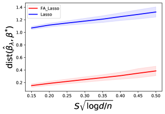
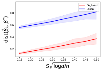
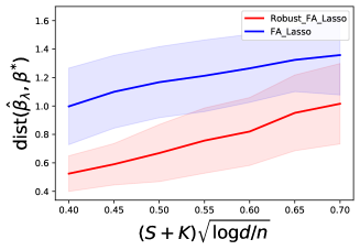
(a)	(b)	(c)

Figure 1: Accuracy for $\widehat{\beta}_{\lambda}$ with dist$(\widehat{\beta}_{\lambda},\beta^{\star}):=\|\widehat{\beta}_{\lambda}-\beta^{\star}\|_{1}$ based on 500 replications. The light color regions indicate the standard errors across the simulation. Figure (a) and (b) depict the estimation results of model (1.5) with noise $\epsilon$ following the standard Gaussian and uniform distributions respectively. In (a) and (b), the red lines denote the estimation results using the method (2.4) (labeled as FA_Lasso in the figure) and the blue lines represent the results using Lasso with data $(\bm{X},\bm{Y})$. In Figure (c), the noise $\epsilon$ follows $t_{3}$-distribution. The red line in (c) represents the result of robust factor adjusted regression (Robust_FA_Lasso) via adaptive Huber estimation together with $\ell_{1}$-penalty given in (2.7) and the blue line represents the result achieved by using FA_Lasso.

Distributions (i) and (ii) have sub-Gaussian tails. For these two cases, we select sample size $n$ so that $s\sqrt{\log d/n}$ takes uniform grids in $[0.15,0.5]$ . Then we generate $n$ response variables from model (2.1) and estimate our parameters via (2.4). The results are shown as the red lines in Figure 1. They lend further support to our theoretical findings given in section 2 as the statistical rates there are upper bounded by $O(s\sqrt{\log d/n})$. Moreover, we also show the estimation results by using Lasso directly on measurements $(\bm{X},\bm{Y})$. Results are shown as the blue lines given in the first two figures in Figure 1. Using Lasso directly on $(\bm{X},\bm{Y})$ leads to much worse results due in part to the inadequacy of the model. In addition, as shown in Fan et al. (2020a), even when the sparse regression model is correct, we still have better estimation accuracy using factor adjusted regression.

Distribution (iii) has only the bounded second moment. Likewise, we select corresponding number of observations $n$ so that $(s+K)\sqrt{\log d/n}$ takes uniform grids in $[0.4,0.7]$. The reduced sample sizes help reduce the computation cost on the regularized adaptive Huber estimation using cross-validation to choose the parameter $\omega$. We compare the results for the robust estimator (2.7) with that of the factor adjusted regression (2.4). The results are shown as the red and blue lines in part (c) of Figure 1 respectively. They provide stark evidence that it is necessary to conduct the robust version of factor adjusted regression (2.7) when noises have heavy tails.

5.2 Adequacy of Factor Regression

Data Generation Processes. We choose $n=200$, $K=2$ and $d$ either 200 or 500 and the matrix $\bm{X}=\bm{F}\bm{B}^{\top}+\bm{U}$ using the following two models with entries of $\bm{B}$ generated from Unif$(-1,1)$.

1. We generate every row of $\bm{F}\in\mathbb{R}^{n\times K},\bm{U}\in\mathbb{R}^{n\times d}$ from $\textrm{N}(\mathbf{0},\bm{I}_{K})$ and $\textrm{N}(\mathbf{0},\bm{I}_{d})$ respectively.

2. We let the $t$-th row $\bm{f}_{t}\in\mathbb{R}^{K}$ of $\bm{F}\in\mathbb{R}^{n\times K}$ follow $\bm{f}_{t}=\bm{\Phi}\bm{f}_{t-1}+\bm{\xi}_{t}$ where $\bm{\Phi}\in\mathbb{R}^{K\times K}$ with $\bm{\Phi}_{i,j}=0.5^{|i-j|+1},i,j\in[K]$. In addition, $\{\bm{\xi}_{t}\}_{t\geq 1}$ are drawn independently from $\textrm{N}(\textbf{0},\bm{I}_{K})$. We generate every row of $\bm{U}$ from $N(\mathbf{0},\bm{\Sigma})$ where $\Sigma_{i,j}=0.6^{|i-j|},i,j\in[d]$.

The response vector follows $\bm{Y}=\bm{F}\bm{\gamma}^{\star}+\bm{U}\bm{\beta}^{\star}+{\cal E}$ in (4.1) with every entry of ${\cal E}\in\mathbb{R}^{n}$ being generated independently from either from $N(0,0.5^{2})$ or uniform distribution Unif $(-\sqrt{3}/2,\sqrt{3}/2)$. We set $\bm{\gamma}^{\star}=(0.5,0.5)$ and $\bm{\beta}^{\star}=(w,w,w,0,\cdots,0)$, where $w\geq 0$. When $w=0$, the null hypothesis $\bm{Y}=\bm{F}\bm{\gamma}^{\star}+{\cal E}$ holds and the simulation results correpond to the size of the test. Otherwise, they correspond to the power of the test.

Implementation. We summarize the details of the proposed test

1. Estimate factor $\widehat{}\bm{F}$, loading matrix $\widehat{}\bm{B}$, and noise $\widehat{}\bm{U}$ as in section 2.

2. For the given $\widehat{}\bm{U},$ we estimate $\widehat{}\bm{\Theta}$ by using node-wise regression (van de Geer et al., 2014).

3. Use Lasso method to estimate $\widehat{}\bm{\beta}_{\lambda}$ based on data $(\widehat{}\bm{U},\widetilde{\bm{Y}})$ with $\lambda$ chosen by cross-validation.

4. Construct a de-biased $\widetilde{\bm{\beta}}_{\lambda}=\widehat{\bm{\beta}}_{\lambda}+n^{-1}\widehat{\bm{\Theta}}\widehat{\bm{U}}^{\top}(\bm{Y}-\widehat{\bm{U}}\widehat{\bm{\beta}}_{\lambda})$ .

5. Obtain $\widehat{L}=1/\sqrt{n}\|\widehat{}\bm{\Theta}\widehat{}\bm{U}^{\top}\widetilde{{\cal E}}\|_{\infty}$ with every entry of $\widetilde{{\cal E}}$ simulated from $N(0,1)$ and repeat this computation $1000$ times to obtain the upper-$\alpha$ quantile $\widehat{c}_{1-\alpha}$ of $\widehat{L}$.

6. Compute the test result $\xi_{\alpha}:=\mathbb{I}\{\sqrt{n}\|\widetilde{\bm{\beta}}_{\lambda}\|_{\infty}/\widehat{\sigma}>\widehat{c}_{1-\alpha}\}$ where $\widehat{\sigma}$ is estimated by using refitted cross-validation (Fan et al., 2012).

The size and the power are then calculated based on 2000 simulations with $\alpha=0.05$ .

Results. For $n=200,K=2$, $d\in\{200,500\}$ and all $w\in\{0,0.05,0.10,0.15,0.20\}$, we generate the data from each model and compute the testing results based on 2000 simulaitons with $\alpha=0.05$. The results are depicted in the Table 1. The column named Gaussian$(i)$, $i\in\{1,2\}$ represents the simulation results under model $i$ with Gaussian noise. Similar labels applied to the uniform noise distribution.

		Gaussian (1)	Gaussian (2)	Uniform (1)	Uniform (2)
$p=200$	$w=0$	$0.044$	$0.047$	$0.046$	$0.048$
	$w=0.05$	$0.067$	$0.119$	$0.065$	$0.108$
	$w=0.10$	$0.326$	$0.714$	$0.311$	$0.653$
	$w=0.15$	$0.859$	$0.989$	$0.854$	$0.984$
	$w=0.20$	$0.998$	$1.000$	$0.996$	$1.000$
$p=500$	$w=0$	$0.043$	$0.040$	$0.048$	$0.436$
	$w=0.05$	$0.067$	$0.080$	$0.059$	$0.071$
	$w=0.10$	$0.253$	$0.632$	$0.237$	$0.563$
	$w=0.15$	$0.787$	$0.974$	$0.780$	$0.962$
	$w=0.20$	$0.993$	$1.000$	$0.987$	$1.000$

Table 1: Simulation results of section 3 under different regimes.

Table 1 reveals that our test gives approximately the right size (subject to simulation error; see the rows with $w=0$). This is consistent with our theoretical findings given in section 3. In addition, when $0<w<0.2$, the power of our test increases rapidly to $1$ which reveals the efficiency of our test statistic.

5.3 Adequacy of Sparse Regression

This subsection provides finite-sample validations for the results in section 4. We take the number of data used for screening $m=\lceil n^{0.8}\rceil$, use Iterative Sure Independence Screening method (Fan and Lv, 2008; Saldana and Feng, 2018; Zhang et al., 2019) to select $\widehat{{\cal S}}_{1}$ and apply the refitted cross-validation (Fan et al., 2012) to estimate $\sigma^{2}$. The size and the power of the test are computed based on 2000 simulations.

Data Generation Processes. We let $n=250$, $K=3$ and $d$ be either $250$ or $600$. The noises $\varepsilon$ are i.i.d from $N(0,0.5^{2})$ or Unif $(-\sqrt{3}/2,\sqrt{3}/2)$. The covariate $\bm{X}\in\mathbb{R}^{n\times d}$ follows the factor model $\bm{X}=\bm{F}\bm{B}^{\top}+\bm{U}$. We generate $\bm{F},$ $\bm{U}$ and $\bm{B}$ in the same way as those in section 5.2. In addition, the response variable follows $\bm{Y}=\bm{F}\bm{\varphi}^{\star}+\bm{X}\bm{\beta}^{\star}+{\cal E}$ in (4.1) with $\bm{\beta}^{\star}=(0.8,0.8,0.8,0.8,0,\cdots,0)$ and $\bm{\varphi}^{\star}=v\cdot\mathbf{1}_{K\times 1}$ for several different values of $v\geq 0$. The case $v=0$ corresponds to the null hypothesis and it is designed to test the validity of the size.

Results. For $n=250$, $K=3$, $d\in\{250,600\}$ and $v\in\{0,0.04,0.08,0.12,0.16\}$, we implement the proposed method for every model in section 5.2. The simulation results are depicted in Table 2. The column named Gaussian (or uniform) $(i)$, $i\in\{1,2\}$ represents the results under model $i$ with Gaussian (or uniform) noise mentioned in section 5.2. When $v=0$, the null hypothesis holds, our Type-I error is approximately $0.05$ which matches with the theoretical value. In addition, when we increase the size of $v$ from $v=0.04$ to $v=0.16$, the power of our test statistic increases sharply to $1$, which reveals its efficiency.

		Gaussian (1)	Gaussian (2)	Uniform (1)	Uniform (2)
$p=250$	$v=0$	$0.051$	$0.054$	$0.056$	$0.053$
	$v=0.04$	$0.215$	$0.278$	$0.233$	$0.286$
	$v=0.08$	$0.659$	$0.740$	$0.655$	$0.750$
	$v=0.12$	$0.965$	$0.993$	$0.965$	$0.996$
	$v=0.16$	$1.000$	$1.000$	$1.000$	$1.000$
$p=600$	$v=0$	$0.051$	$0.052$	$0.050$	$0.052$
	$v=0.04$	$0.208$	$0.362$	$0.197$	$0.353$
	$v=0.08$	$0.624$	$0.802$	$0.604$	$0.785$
	$v=0.12$	$0.941$	$0.994$	$0.934$	$0.999$
	$v=0.16$	$1.000$	$1.000$	$0.999$	$1.000$

Table 2: Simulation results of section 4 under different regimes.

We next discuss the necessity of using sample splitting. Suppose we do not split samples and use the whole dataset to do sure screening and construct the test statistic. This will result in the high correlation between the selected set $\widehat{{\cal S}}$ and covariates when $\widehat{{\cal S}}$ is not a consistent estimator of ${\cal S}_{\star}$. In this case, the asymptotic behavior of our test statistic is hard to capture. To demonstrate this point, we simulate the null distribution of the test statistic constructed without using sample splitting and compare it with the asymptotic distribution ($\chi_{K}^{2}$) via the quantile-quantile plot in Figure 2. Figure 2 reveals that the test statistic constructed without using sample splitting has heavier right tail than that of the $\chi_{K}^{2}$ distribution. The sizes of the test are much larger than the results in Table 2 when $v=0$.

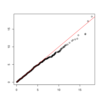
Figure 2: Quantiles of the $\chi_{K}^{2}$ distribution against those of the test statistic without sample splitting. The x-axis represents the quantiles of the test statistic whereas y-axis is the quantiles of $\chi_{K}^{2}$ distribution.

5.4 Empirical Applications

In this section, we use a macroeconomic dataset named FRED-MD (McCracken and Ng, 2016) to illustrate the performance of our factor augmented regression model (FARM) and investigate whether the latent factor regression model and sparse linear model are adequate.

There are 134 monthly U.S. macroeconomic variables in this dataset. As they measure certain aspects of economic health, these variables are driven by latent factors and hence correlated. They can be well explained by a few principal components. In our study, we pick out two variables named ’HOUSTNE’ and ’GS5’ as our responses respectively and let the remaining variables be the covariates. Here ’HOUSTNE’ represents the housing starts in the northeast region and ’GS5’ denotes the $5$-year treasury rate.

There exist significant structural breaks for many variables around the year of financial crisis in 2008 which makes our data non-stationary even after performing the suggested transformations. Thus, we analyze the dataset in two separate time periods independently. Specifically, we study the monthly data collected from February 1992 to October 2007 and from August 2010 to February 2020 respectively after examing the missingness and stationarity of the data.

To illustrate the performance of our proposed FARM against the sparse linear model and latent factor regression model, we first analyze the prediction results achieved by using these models. For every given time period and model, we perform the prediction by using the moving window approach with window size 90 months. Indexing the panel data from 1 for each of the two time periods, for all $t>90$, we use the 90 previous measurements $\{(\bm{x}_{t-90},Y_{t-90}),\cdots,(\bm{x}_{t-1},Y_{t-1})\}$ to train a model (FARM, sparse linear regression model, or latent factor regression model) and output a prediction $\widehat{Y}_{t}$ as well as the in-sample average $\bar{Y}_{t}:=\frac{1}{90}\sum_{i=t-90}^{t-1}Y_{i}$. We measure the prediction accuracy by using out-of-sample $R^{2}$:

$$R^{2}=1-\frac{\sum_{t=91}^{T}(Y_{t}-\widehat{Y}_{t})^{2}}{\sum_{t=91}^{T}(Y_{t}-\bar{Y}_{t})^{2}},$$

where $T$ denotes the number of total data points in a given time period. Table 3 presents the out-of-sample $R^{2}$ obtained by the aforementioned three models in the two time periods for predicting ’HOUSTNE’ and ’GS5’. Their detailed predictions are depicted in Figure 3 and Figure 4 respectively. Both out-of-sample $R^{2}$ and predictions depicted in Figures 3 and 4 show that FARM outperforms both latent factor regression and sparse linear regression models.

Time period	Data	FARM	SP_Linear	LA_Factor
02.1992-10.2007	HOUSTNE	$0.632$	$0.584$	$0.428$
	GS5	$0.705$	$0.631$	$0.122$
08.2010-02.2020	HOUSTNE	$0.694$	$0.450$	$0.219$
	GS5	$0.657$	$0.540$	$0.233$

Table 3: Out-of-sample $R^{2}$ for predicting ’HOUSTNE’ and ’GS5’ data using different models in different time periods. LA_Factor and SP_Linear stand for latent factor regression and sparse linear regression respectively.

We next conduct the hypothesis testing on the adequacy of latent factor regression and sparse linear regression respectively by using FARM as the alternative model. As computing the bootstrap estimate of the null distribution is expensive for testing the adequacy of the factor model, we only conduct the hypothesis testing using the data in the entire two subperiods: 02.1992-10.2007 and 08.2010-02.2020. The P-values for the tests are given in Table 4. Taking the significant level $0.05$, the hypothesis testing results indicate that the latent factor regression is not adequate for all four different settings in Table 4. As for sparse linear regression, it is accepted only for studying ’HOUSTNE’ in the time period 02.1992-10.2007. These results match well with our prediction results.

Time period	Data	LA_factor	SP_Linear
02.1992-10.2007	HOUSTNE	$2.00\cdot 10^{-3}$	$5.75\cdot 10^{-1}$
	GS5	$2.50\cdot 10^{-3}$	$8.73\cdot 10^{-3}$
08.2010-02.2020	HOUSTNE	$<10^{-3}$	$2.00\cdot 10^{-2}$
	GS5	$1.70\cdot 10^{-2}$	$2.94\cdot 10^{-2}$

Table 4: $p$-values for testing the adequacy of the latent factor regression and sparse linear regression models to explain ’HOUSTNE’ and ’GS5’ data in two different time periods. The LA_Factor and SP_Linear have the same meaning as those in Table 3.

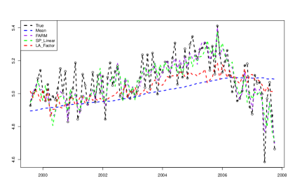
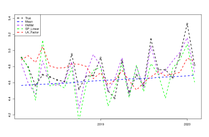
Figure 3: Out-of-sample prediction results for ’HOUSTNE’ data in time periods: August 1999 to October 2007 (left panel) and Februrary 2018 to February 2020 (right panel). The black dash line represents the true observed values, and the blue, purple, green and red dash lines represent the predictions made by using in-sample mean (moving average with a window of 90), FARM, sparse linear model and latent factor regression model, respectively.

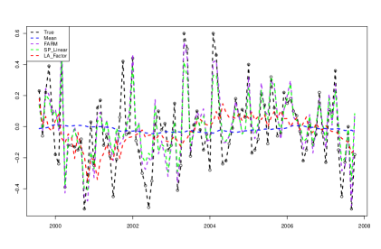
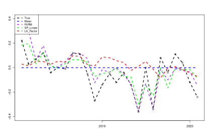
Figure 4: Out-of-sample prediction results for ’GS5’ data in time periods: August 1999 to October 2007 (left panel) and Februrary 2018 to February 2020 (right panel). The same captions as those in Figure 3 are used.

6 Conclusion

In this paper, we propose a model named Factor Augmented sparse linear Regression Model (FARM), which contains the latent factor regression and the sparse linear regression as our special cases. The model expands the space spanned by covariates into useful directions and hence use additional information beyond the linear space spanned by the predictors. We provide theoretical guarantees for our model estimation under the existence of light-tailed and heavy-tailed noises respectively. In addition, we leverage our model as the alternative one to test the sufficiency of the latent factor regression model and sparse regression model. We believe that the study is among the first of this kind. The practical performance of our model estimation and our constructed test statistics are proven by extensive simulation studies including both synthetic data and real data. Moreover, it is worth to mention that our model and methodology can be extended to more general supervised learning problems such as nonparametric regression, quantile regression, regression and classification trees, support vector machines, among others where the factor augmentation idea is always useful.

References

- Ahn and Horenstein [2013] S. C. Ahn and A. R. Horenstein. Eigenvalue ratio test for the number of factors. Econometrica, 81(3):1203–1227, 2013.
- Avella-Medina et al. [2018] M. Avella-Medina, H. S. Battey, J. Fan, and Q. Li. Robust estimation of high-dimensional covariance and precision matrices. Biometrika, 105(2):271–284, 2018.
- Bai [2003] J. Bai. Inferential theory for factor models of large dimensions. Econometrica, 71(1):135–171, 2003.
- Bai and Li [2012] J. Bai and K. Li. Statistical analysis of factor models of high dimension. Ann. Statist., 40(1):436–465, 2012.
- Bai and Ng [2002] J. Bai and S. Ng. Determining the number of factors in approximate factor models. Econometrica, 70(1):191–221, 2002.
- Bai and Ng [2006] J. Bai and S. Ng. Confidence intervals for diffusion index forecasts and inference for factor-augmented regressions. Econometrica, 74(4):1133–1150, 2006.
- Bai and Ng [2008] J. Bai and S. Ng. Forecasting economic time series using targeted predictors. Journal of Econometrics, 146(2):304–317, 2008. ISSN 0304-4076.
- Bair et al. [2006] E. Bair, T. Hastie, D. Paul, and R. Tibshirani. Prediction by supervised principal components. Journal of the American Statistical Association, 101(473):119–137, 2006.
- Barut et al. [2016] E. Barut, J. Fan, and A. Verhasselt. Conditional sure independence screening. J. Amer. Statist. Assoc., 111(515):1266–1277, 2016.
- Belloni and Chernozhukov [2011] A. Belloni and V. Chernozhukov. -penalized quantile regression in high-dimensional sparse models. Ann. Statist., 39(1):82–130, 2011.
- Bing et al. [2019] X. Bing, F. Bunea, and M. Wegkamp. Inference in latent factor regression with clusterable features. arXiv:1905.12696, 2019.
- Bing et al. [2021] X. Bing, F. Bunea, S. Strimas-Mackey, and M. Wegkamp. Prediction under latent factor regression: Adaptive pcr, interpolating predictors and beyond. Journal of Machine Learning Research, 22(177):1–50, 2021.
- Bunea et al. [2020] F. Bunea, S. Strimas-Mackey, and M. Wegkamp. Interpolating predictors in high-dimensional factor regression. arXiv:2002.02525, 2020.
- Cai et al. [2011] T. Cai, W. Liu, and X. Luo. A constrained minimization approach to sparse precision matrix estimation. J. Amer. Statist. Assoc., 106(494):594–607, 2011.
- Candes and Tao [2007] E. Candes and T. Tao. The Dantzig selector: statistical estimation when is much larger than . Ann. Statist., 35(6):2313–2351, 2007.
- Chernozhukov et al. [2013] V. Chernozhukov, D. Chetverikov, and K. Kato. Gaussian approximations and multiplier bootstrap for maxima of sums of high-dimensional random vectors. Ann. Statist., 41(6):2786–2819, 2013.
- Chernozhukov et al. [2017] V. Chernozhukov, D. Chetverikov, and K. Kato. Central limit theorems and bootstrap in high dimensions. Ann. Probab., 45(4):2309–2352, 2017.
- Chernozhukov et al. [2020] V. Chernozhukov, D. Chetverikov, and Y. Koike. Nearly optimal central limit theorem and bootstrap approximations in high dimensions. arXiv preprint arXiv:2012.09513, 2020.
- Chu et al. [2016] W. Chu, R. Li, and M. Reimherr. Feature screening for time-varying coefficient models with ultrahigh dimensional longitudinal data. Ann. Appl. Stat., 10(2):596, 2016.
- Dezeure et al. [2017] R. Dezeure, P. Bühlmann, and C.-H. Zhang. High-dimensional simultaneous inference with the bootstrap. Test, 26(4):685–719, 2017.
- Efron et al. [2004] B. Efron, T. Hastie, I. Johnstone, and R. Tibshirani. Least angle regression. Ann. Statist., 32(2):407–499, 2004.
- Fan and Li [2001] J. Fan and R. Li. Variable selection via nonconcave penalized likelihood and its oracle properties. J. Amer. Statist. Assoc., 96(456):1348–1360, 2001.
- Fan and Liao [2020] J. Fan and Y. Liao. Learning latent factors from diversified projections and its applications to over-estimated and weak factors. Journal of the American Statistical Association, 0(0):1–16, 2020.
- Fan and Lv [2008] J. Fan and J. Lv. Sure independence screening for ultrahigh dimensional feature space. J. R. Stat. Soc. Ser. B Stat. Methodol., 70(5):849–911, 2008.
- Fan and Lv [2011] J. Fan and J. Lv. Nonconcave penalized likelihood with NP-dimensionality. IEEE Trans. Inform. Theory, 57(8):5467–5484, 2011.
- Fan and Song [2010] J. Fan and R. Song. Sure independence screening in generalized linear models with NP-dimensionality. Ann. Statist., 38(6):3567–3604, 2010.
- Fan et al. [2012] J. Fan, S. Guo, and N. Hao. Variance estimation using refitted cross-validation in ultrahigh dimensional regression. J. R. Stat. Soc. Ser. B. Stat. Methodol., 74(1):37–65, 2012.
- Fan et al. [2013] J. Fan, Y. Liao, and M. Mincheva. Large covariance estimation by thresholding principal orthogonal complements. J. R. Stat. Soc. Ser. B. Stat. Methodol., 75(4):603–680, 2013. With 33 discussions by 57 authors and a reply by Fan, Liao and Mincheva.
- Fan et al. [2014] J. Fan, Y. Fan, and E. Barut. Adaptive robust variable selection. Ann. Statist., 42(1):324, 2014.
- Fan et al. [2017a] J. Fan, Q. Li, and Y. Wang. Estimation of high dimensional mean regression in the absence of symmetry and light tail assumptions. J. R. Stat. Soc. Ser. B Stat. Methodol., 79(1):247, 2017a.
- Fan et al. [2017b] J. Fan, L. Xue, and j. Yao. Sufficient forecasting using factor models. Journal of Econometrics, 201(2):292–306, 2017b. ISSN 0304-4076.
- Fan et al. [2020a] J. Fan, Y. Ke, and K. Wang. Factor-adjusted regularized model selection. J. Econometrics, 216(1):71–85, 2020a.
- Fan et al. [2020b] J. Fan, R. Li, C.-H. Zhang, and H. Zou. Statistical foundations of data science. 2020b.
- Fan et al. [2021a] J. Fan, J. Guo, and S. Zheng. Estimating number of factors by adjusted eigenvalues thresholding. Journal of the American Statistical Association, pages 1–10, 2021a.
- Fan et al. [2021b] J. Fan, R. Masini, and M. C. Medeiros. Bridging factor and sparse models. arXiv:2102.11341, 2021b.
- Fan et al. [2021c] J. Fan, Z. Yang, and M. Yu. Understanding implicit regularization in over-parameterized single index model. arXiv:2007.08322v3, 2021c.
- Hernan and Robins [2019] M. Hernan and J. Robins. Causal Inference. Chapman & Hall/CRC Monographs on Statistics & Applied Probab. CRC Press LLC, 2019. ISBN 9781420076165.
- Hotelling [1933] H. Hotelling. Analysis of a complex of statistical variables into principal components. Journal of educational psychology, 24(6):417, 1933.
- Imbens and Rubin [2015] G. Imbens and D. Rubin. Causal inference for statistics, social, and biomedical sciences: An introduction. 2015.
- Javanmard and Montanari [2014] A. Javanmard and A. Montanari. Confidence intervals and hypothesis testing for high-dimensional regression. J. Mach. Learn. Res., 15:2869–2909, 2014.
- Jolliffe [1982] I. T. Jolliffe. A note on the use of principal components in regression. Journal of the Royal Statistical Society. Series C (Applied Statistics), 31(3):300–303, 1982.
- Lam and Yao [2012] C. Lam and Q. Yao. Factor modeling for high-dimensional time series: Inference for the number of factors. The Annals of Statistics, 40(2):694 – 726, 2012.
- Li et al. [2012] G. Li, H. Peng, J. Zhang, and L. Zhu. Robust rank correlation based screening. Ann. Statist., 40(3):1846–1877, 2012.
- Li and Li [2021] Q. Li and L. Li. Integrative factor regression and its inference for multimodal data analysis. J. Amer. Statist. Assoc., 113(521):1–15, 2021.
- Li et al. [2018] Q. Li, G. Cheng, J. Fan, and Y. Wang. Embracing the blessing of dimensionality in factor models. J. Amer. Statist. Assoc., 113(521):380–389, 2018.
- Liu et al. [2014] J. Liu, R. Li, and R. Wu. Feature selection for varying coefficient models with ultrahigh-dimensional covariates. J. Amer. Statist. Assoc., 109(505):266–274, 2014.
- Loh and Wainwright [2012] P.-L. Loh and M. J. Wainwright. High-dimensional regression with noisy and missing data: Provable guarantees with nonconvexity. Ann. Statist., 40(3):1637–1664, 2012.
- McCracken and Ng [2016] M. W. McCracken and S. Ng. Fred-md: A monthly database for macroeconomic research. Journal of Business & Economic Statistics, 34(4):574–589, 2016.
- Nickl and Van De Geer [2013] R. Nickl and S. Van De Geer. Confidence sets in sparse regression. Ann. Statist., 41(6):2852–2876, 2013.
- Peng et al. [2016] B. Peng, L. Wang, and Y. Wu. An error bound for -norm support vector machine coefficients in ultra-high dimension. J. Mach. Learn. Res., 17(1):8279–8304, 2016.
- Saldana and Feng [2018] D. F. Saldana and Y. Feng. Sis: An r package for sure independence screening in ultrahigh-dimensional statistical models. Journal of Statistical Software, 83(2):1–25, 2018.
- Shi et al. [2019] C. Shi, R. Song, Z. Chen, and R. Li. Linear hypothesis testing for high dimensional generalized linear models. Ann. Statist., 47(5):2671–2703, 2019.
- Stock and Watson [2002] J. H. Stock and M. W. Watson. Forecasting using principal components from a large number of predictors. Journal of the American Statistical Association, 97(460):1167–1179, 2002.
- Sun et al. [2020] Q. Sun, W.-X. Zhou, and J. Fan. Adaptive Huber regression. Journal of the American Statistical Association, 115(529):254–265, 2020.
- Sun and Zhang [2012] T. Sun and C.-H. Zhang. Scaled sparse linear regression. Biometrika, 99(4):879–898, 2012.
- Tibshirani [1996] R. Tibshirani. Regression shrinkage and selection via the lasso. J. Roy. Statist. Soc. Ser. B, 58(1):267–288, 1996.
- Van de Geer [2008] S. Van de Geer. High-dimensional generalized linear models and the lasso. Ann. Statist., 36(2):614–645, 2008.
- van de Geer et al. [2014] S. van de Geer, P. Bühlmann, Y. Ritov, and R. Dezeure. On asymptotically optimal confidence regions and tests for high-dimensional models. Ann. Statist., 42(3):1166–1202, 2014.
- Wang and Fan [2017] W. Wang and J. Fan. Asymptotics of empirical eigenstructure for high dimensional spiked covariance. Ann. Statist., 45(3):1342–1374, 2017.
- Wang and Leng [2016] X. Wang and C. Leng. High dimensional ordinary least squares projection for screening variables. J. R. Stat. Soc. Ser. B Stat. Methodol., pages 589–611, 2016.
- Yu and Bien [2019] G. Yu and J. Bien. Estimating the error variance in a high-dimensional linear model. Biometrika, 106(3):533–546, 2019.
- Zhang [2010] C.-H. Zhang. Nearly unbiased variable selection under minimax concave penalty. Ann. Statist., 38(2):894–942, 2010.
- Zhang and Zhang [2014] C.-H. Zhang and S. S. Zhang. Confidence intervals for low dimensional parameters in high dimensional linear models. J. R. Stat. Soc. Ser. B. Stat. Methodol., 76(1):217–242, 2014.
- Zhang et al. [2019] N. Zhang, W. Jiang, and Y. Lan. On the sure screening properties of iteratively sure independence screening algorithms. arXiv:1812.01367, 2019.
- Zhang and Cheng [2017] X. Zhang and G. Cheng. Simultaneous inference for high-dimensional linear models. J. Amer. Statist. Assoc., 112(518):757–768, 2017.
- Zhang et al. [2016] X. Zhang, Y. Wu, L. Wang, and R. Li. Variable selection for support vector machines in moderately high dimensions. J. R. Stat. Soc. Ser. B Stat. Methodol., 78(1):53, 2016.
- Zhao and Yu [2006] P. Zhao and B. Yu. On model selection consistency of Lasso. J. Mach. Learn. Res., 7:2541–2563, 2006.
- Zhao et al. [2019] P. Zhao, Y. Yang, and Q.-C. He. Implicit regularization via hadamard product over-parametrization in high-dimensional linear regression. arXiv:1903.09367, 2019.
- Zhu et al. [2011] L.-P. Zhu, L. Li, R. Li, and L.-X. Zhu. Model-free feature screening for ultrahigh-dimensional data. J. Amer. Statist. Assoc., 106(496):1464–1475, 2011.
- Zou [2006] H. Zou. The adaptive lasso and its oracle properties. J. Amer. Statist. Assoc., 101(476):1418–1429, 2006.